arX

iv:m

ath/

0407

174v

1 [m

ath.

HO

] 10

Jul

200

4 Totally real origami andimpossible paper folding

David Auckly and John Cleveland

Department of MathematicsThe University of Texas at Austin

Austin, TX 78712

Origami is the ancient Japanese art of paper folding. It is possible to fold many

intriguing geometrical shapes with paper [M]. In this article, the question we will answer

is which shapes are possible to construct and which shapes are impossible to construct

using origami. One of the most interesting things we discovered is that it is impossible

to construct a cube with twice the volume of a given cube using origami, just as it is

impossible to do using a compass and straight edge. As an unexpected surprise, our

algebraic characterization of origami is related to David Hilbert’s 17th problem. Hilbert’s

problem is to show that any rational function which is always non-negative is a sum of

squares of rational functions [B]. This problem was solved by Artin in 1926 [Ar]. We would

like to thank John Tate for noticing the relationship between our present work and Hilbert’s

17th problem. This research is the result of a project in the Junior Fellows Program at

The University of Texas. The Junior Fellows Program is a program in which a junior

undergraduate strives to do original research under the guidance of a faculty mentor.

The referee mentioned two references which the reader may find interesting. “Geomet-

ric Exercises in Paper Folding” addresses practical problems of paper folding [R]. Among

many other things, Sundara Row gives constructions for the 5-gon, the 17-gon, and dupli-

cating a cube. His constructions, however, use more general folding techniques than the

ones we consider here. Felix Klein cites Row’s work in his lectures on selected questions

in elementary geometry [K].

In order to understand the rules of origami construction, we will first consider a sheet

of everyday notebook paper. Our work with notebook paper will serve as an intuitive

model for our definition of origami constructions in the Euclidean plane. There are four

1

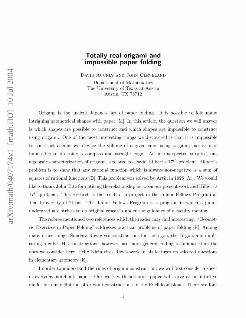
natural methods of folding a piece of paper. The methods will serve as the basis of the

definition of an origami pair.

δ

1

L

L

2

3

α β

γ

L

Figure 1

We construct the line L1, by folding a crease between two different corners of the paper.

Another line may be constructed by matching two corners. For example, if corners α and

γ are matched, the crease formed, L2, will be the perpendicular bisector of the segment

αγ. another natural construction is matching one line to another line. For instance, βγ,

the paper’s edge, and L2 are lines. If we lay βγ upon L2 and form the crease, then we

obtain L3 which is the angle bisector of the two lines. If we start with two parallel lines

in this third construction, then we will just get a parallel line half way in between.

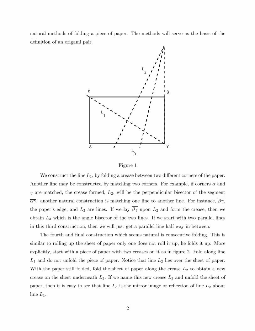
The fourth and final construction which seems natural is consecutive folding. This is

similar to rolling up the sheet of paper only one does not roll it up, he folds it up. More

explicitly, start with a piece of paper with two creases on it as in figure 2. Fold along line

L1 and do not unfold the piece of paper. Notice that line L2 lies over the sheet of paper.

With the paper still folded, fold the sheet of paper along the crease L2 to obtain a new

crease on the sheet underneath L2. If we name this new crease L3 and unfold the sheet of

paper, then it is easy to see that line L3 is the mirror image or reflection of line L2 about

line L1.

2

2

L L1 2

L3

L L1 2 L1

L

Figure 2

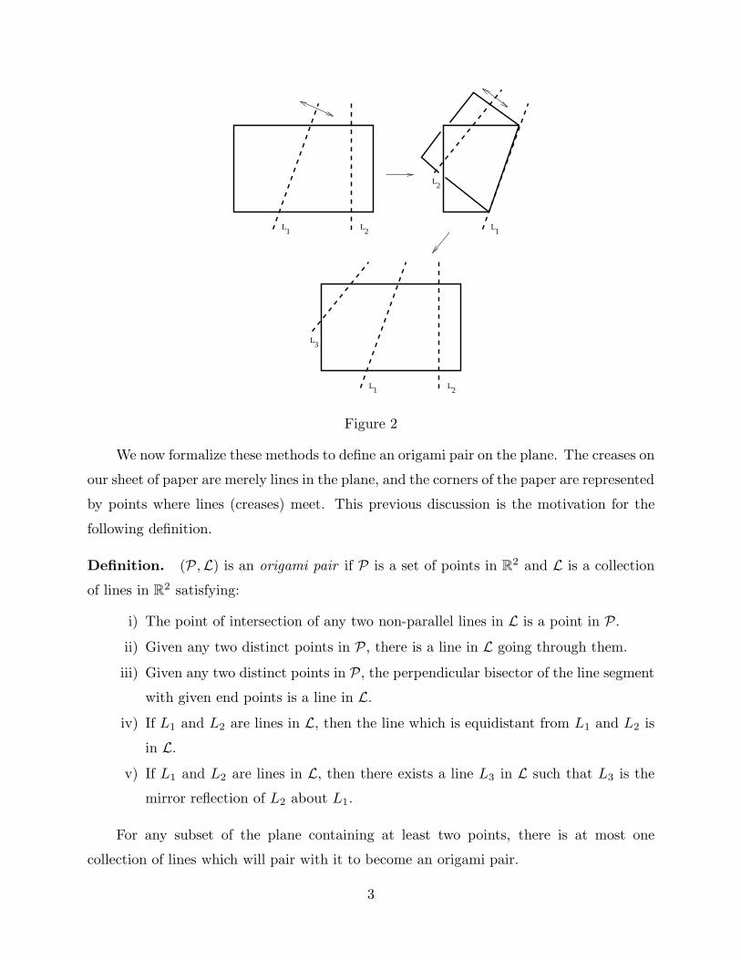
We now formalize these methods to define an origami pair on the plane. The creases on

our sheet of paper are merely lines in the plane, and the corners of the paper are represented

by points where lines (creases) meet. This previous discussion is the motivation for the

following definition.

Definition. (P,L) is an origami pair if P is a set of points in R2 and L is a collection

of lines in R2 satisfying:

i) The point of intersection of any two non-parallel lines in L is a point in P.

ii) Given any two distinct points in P, there is a line in L going through them.

iii) Given any two distinct points in P, the perpendicular bisector of the line segment

with given end points is a line in L.

iv) If L1 and L2 are lines in L, then the line which is equidistant from L1 and L2 is

in L.

v) If L1 and L2 are lines in L, then there exists a line L3 in L such that L3 is the

mirror reflection of L2 about L1.

For any subset of the plane containing at least two points, there is at most one

collection of lines which will pair with it to become an origami pair.

3

Definition. A subset of R2,P, is closed under origami constructions if there exists a

collection of lines, L, such that (P,L) is an origami pair.

The question which we answer in this paper is which points may be constructed from

just two points, using only the origami constructions described above. We will call that

collection of points the set of origami constructible points.

Definition. P0 = ∩{P | (0, 0), (0, 1) ∈ P and P is closed under origami constructions}is the set of origami constructible points.

Before we explain the structure of P0, we give an example of an origami construction

analogous to many compass and straight edge constructions, namely, the construction of

parallel lines.

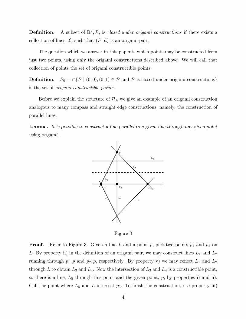
Lemma. It is possible to construct a line parallel to a given line through any given point

using origami.

6

p1 p3 p2

p

L

L1

L2

L3 L4L5

L

Figure 3

Proof. Refer to Figure 3. Given a line L and a point p, pick two points p1 and p2 on

L. By property ii) in the definition of an origami pair, we may construct lines L1 and L2

running through p1, p and p2, p, respectively. By property v) we may reflect L1 and L2

through L to obtain L3 and L4. Now the intersection of L3 and L4 is a constructible point,

so there is a line, L5 through this point and the given point, p, by properties i) and ii).

Call the point where L5 and L intersect p3. To finish the construction, use property iii)

4

to construct a perpendicular bisector to p, p3, and reflect L through this bisector with

property v) to obtain the desired line, L6. It is a straightforward exercise to show that L6

has the desired properties.

The reader may wish to try some constructions on his own. Two especially interesting

exercises to attempt are the construction of a right triangle with given legs and the con-

struction of a right triangle with a given hypotenuse and leg. More explicitly, given four

distinct points α, β, γ and δ, the reader may try to construct a point ε such that α, β, ε

are the vertices of a right triangle with legs αβ and βε such that the length of βε equals

the length of γδ.

Now that we have a better feel for origami constructions, we will start developing

tools to show that some figures are not constructible. The first thing we need is the notion

of an origami number.

Definition. F0 = {α ∈ R | ∃ v1, v2 ∈ P such that |α| = dist(v1, v2)} is the set of origami

numbers.

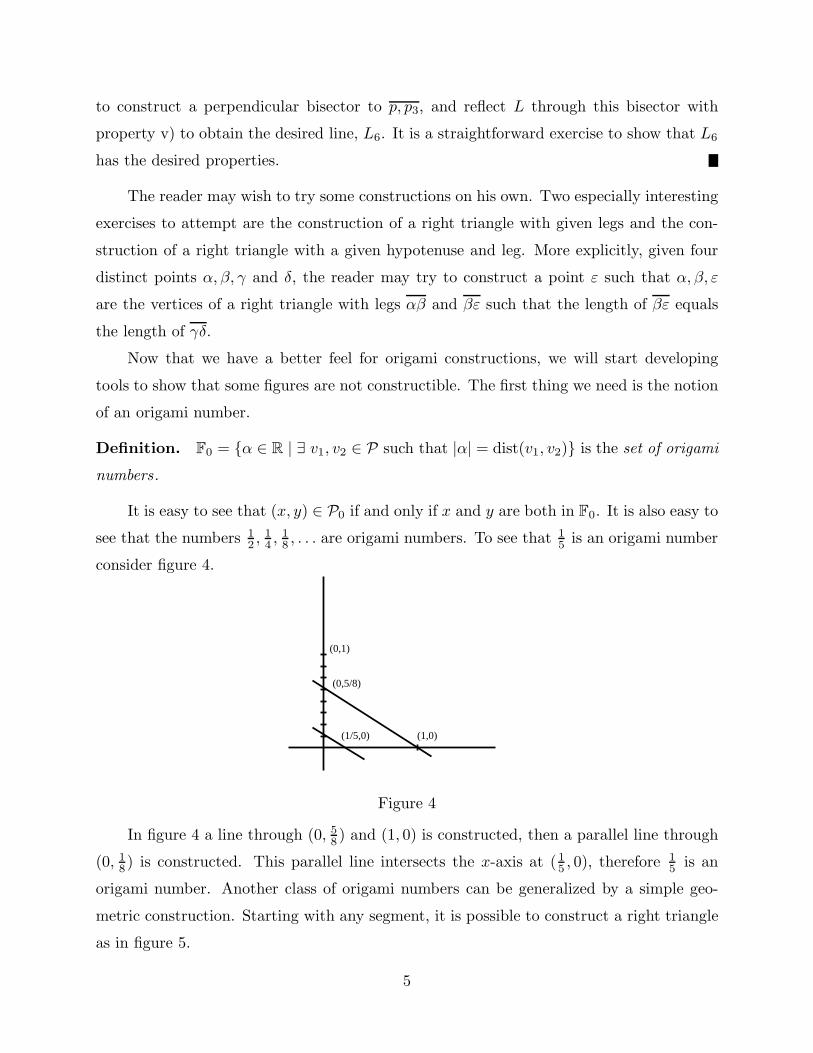
It is easy to see that (x, y) ∈ P0 if and only if x and y are both in F0. It is also easy to

see that the numbers 12 , 1

4 , 18 , . . . are origami numbers. To see that 1

5 is an origami number

consider figure 4.

(1,0)

(0,1)

(0,5/8)

(1/5,0)

Figure 4

In figure 4 a line through (0, 58 ) and (1, 0) is constructed, then a parallel line through

(0, 18) is constructed. This parallel line intersects the x-axis at ( 1

5 , 0), therefore 15 is an

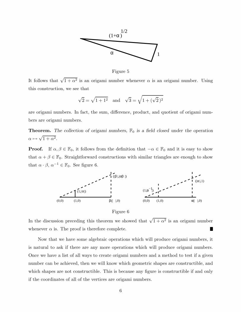
origami number. Another class of origami numbers can be generalized by a simple geo-

metric construction. Starting with any segment, it is possible to construct a right triangle

as in figure 5.

5

1

1/2

α

(1+ )α

Figure 5

It follows that√

1 + α2 is an origami number whenever α is an origami number. Using

this construction, we see that

√2 =

√

1 + 12 and√

3 =

√

1 + (√

2 )2

are origami numbers. In fact, the sum, difference, product, and quotient of origami num-

bers are origami numbers.

Theorem. The collection of origami numbers, F0 is a field closed under the operation

α 7→√

1 + α2.

Proof. If α, β ∈ F0, it follows from the definition that −α ∈ F0 and it is easy to show

that α + β ∈ F0. Straightforward constructions with similar triangles are enough to show

that α · β, α−1 ∈ F0. See figure 6.

(0,0) (1,0) (| |,0)

(| |,1)

(0,0) (1,0) (| |,0)

(1,| |)

(| |,| |)

α

β

β αβ

α

α

α

(1,| |)−1

Figure 6

In the discussion preceding this theorem we showed that√

1 + α2 is an origami number

whenever α is. The proof is therefore complete.

Now that we have some algebraic operations which will produce origami numbers, it

is natural to ask if there are any more operations which will produce origami numbers.

Once we have a list of all ways to create origami numbers and a method to test if a given

number can be achieved, then we will know which geometric shapes are constructible, and

which shapes are not constructible. This is because any figure is constructible if and only

if the coordinates of all of the vertices are origami numbers.

6

Definition. F√

1+x2 is the smallest subfield of C closed under the operation x 7→√

1 + x2.

The preceding Theorem may be rephrased as F√

1+x2 ⊂ F0. It is in fact true that

F0 = F√

1+x2 . Thus, the previously listed operations which produce origami numbers are

the only independent operations which produce origami numbers.

Theorem. F0 = F√

1+x2 .

Proof. Since we already know that F√

1+x2 ⊂ F0, we only need to show that F0 ⊂ F√

1+x2 .

That is, we need to show that any origami number may be expressed using the usual field

operations and the operation x 7→√

1 + x2. It is enough to consider the coordinates of

origami constructible points, because a number is an origami number if and only if it is

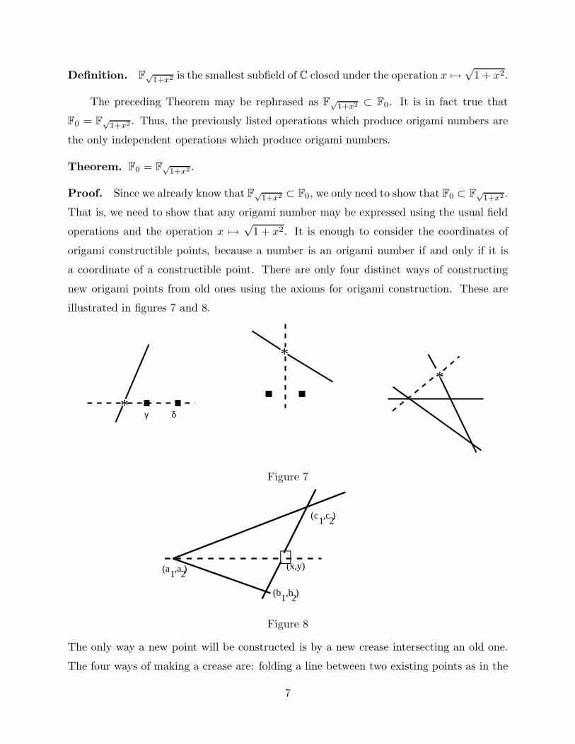
a coordinate of a constructible point. There are only four distinct ways of constructing

new origami points from old ones using the axioms for origami construction. These are

illustrated in figures 7 and 8.

γ δ*

*

*

Figure 7

2

∗ (x,y)1

1

1

(a ,a ) 2

(b ,b ) 2

(c ,c )

Figure 8

The only way a new point will be constructed is by a new crease intersecting an old one.

The four ways of making a crease are: folding a line between two existing points as in the

7

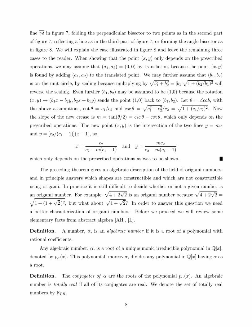
line γδ in figure 7, folding the perpendicular bisector to two points as in the second part

of figure 7, reflecting a line as in the third part of figure 7, or forming the angle bisector as

in figure 8. We will explain the case illustrated in figure 8 and leave the remaining three

cases to the reader. When showing that the point (x, y) only depends on the prescribed

operations, we may assume that (a1, a2) = (0, 0) by translation, because the point (x, y)

is found by adding (a1, a2) to the translated point. We may further assume that (b1, b2)

is on the unit circle, by scaling because multiplying by√

b21 + b2

2 = |b1|√

1 + (b2/b1)2 will

reverse the scaling. Even further (b1, b2) may be assumed to be (1,0) because the rotation

(x, y) 7→ (b1x − b2y, b2x + b1y) sends the point (1,0) back to (b1, b2). Let θ = ∠cab, with

the above assumptions, cot θ = c1/c2 and csc θ =√

c21 + c2

2/c2 =√

1 + (c1/c2)2. Now

the slope of the new crease is m = tan(θ/2) = csc θ − cot θ, which only depends on the

prescribed operations. The new point (x, y) is the intersection of the two lines y = mx

and y = [c2/(c1 − 1)](x − 1), so

x =c2

c2 − m(c1 − 1)and y =

mc2

c2 − m(c1 − 1)

which only depends on the prescribed operations as was to be shown.

The preceding theorem gives an algebraic description of the field of origami numbers,

and in principle answers which shapes are constructible and which are not constructible

using origami. In practice it is still difficult to decide whether or not a given number is

an origami number. For example,√

4 + 2√

2 is an origami number because√

4 + 2√

2 =√

1 + (1 +√

2 )2, but what about√

1 +√

2? In order to answer this question we need

a better characterization of origami numbers. Before we proceed we will review some

elementary facts from abstract algebra [AH], [L].

Definition. A number, α, is an algebraic number if it is a root of a polynomial with

rational coefficients.

Any algebraic number, α, is a root of a unique monic irreducible polynomial in Q[x],

denoted by pα(x). This polynomial, moreover, divides any polynomial in Q[x] having α as

a root.

Definition. The conjugates of α are the roots of the polynomial pα(x). An algebraic

number is totally real if all of its conjugates are real. We denote the set of totally real

numbers by FTR.

8

Of the numbers which we are using to motivate this section,√

4 + 2√

2 is totally

real, because all of its conjugates (±√

4 ± 2√

2 ) are real, but√

1 +√

2 is not totally real

because two of its conjugates are imaginary (±√

1 −√

2 ).

The last topic which we review is symmetric polynomials. The symmetric group on n

letters acts on polynomials in n variables by σf(x1, x2, . . . , xn) = f(xσ(1), xσ(2), . . . , xσ(n))

where f ∈ R[x1, . . . , xn] and R is an arbitrary ring.

Definition. The fixed points of the above action are called symmetric polynomials over

R.

For example, x21 + x2

2 is a symmetric polynomial in two variables because it remains

unchanged when the variables are interchanged. However, x21 − x2

2 is not a symmetric

polynomial because it becomes x22 − x2

1 6= x21 − x2

2 when x1 and x2 are interchanged. One

important class of symmetric polynomials is the class of elementary symmetric polynomials.

Definition. If∏n

k=1(t + xk) is expanded, we obtain

n∏

k=1

(t + xk) =n

∑

ℓ=0

σℓ(x1, . . . , xn)tn−ℓ .

The σℓ(x1, . . . , xn) are the elementary symmetric polynomials.

It is easily verify that

σ1 = x1 + x2 + · · ·+ xn

σℓ = the sum of all products of ℓ distinct xk’s

σn = x1 · x2 · · ·xn.

Fact. [L, page 191]. The algebra of symmetric polynomials over R is generated by

the elementary symmetric polynomials. That is, any symmetric polynomial is a linear

combination of products of the elementary symmetric polynomials.

We will now begin the final characterization of the origami numbers. It happens that

all origami numbers are totally real. To prove this, it is necessary to show that the sum,

difference, product and quotient of totally real numbers is totally real, and that√

1 + α2

is totally real whenever α is totally real. This is proven by using symmetric polynomials

and the following lemma.

9

Lemma.n

∏

i=1

m∏

j=1

(t − xiyj) = det(tI − AB)

where A and B are matrices with entries expressed in terms of the elementary symmetric

polynomials of xi or yj respectively.

This lemma is interesting because it is easier to prove a more general statement which

implies the lemma than it is to verify the lemma. We will prove the lemma when the

xi and yj are independent variables, a more general statement than when the xi and yj

represent numbers, but, nevertheless, an easier statement to prove.

Proof. Let

PA(t) =n

∏

k=1

(t − xk) =n

∑

ℓ=0

(−1)ℓσℓ(x)tn−ℓ

and

PB(t) =n

∏

j=1

(t − yj) =m

∑

j=0

(−1)jσj(y)tm−j .

Let

Vk,ℓ =

1xk

x2k

...xn−1

k

yℓ

xkyℓ

...xn−1

k yℓ

...ym−1

ℓ

xkyn−1ℓ

...xn−1

k yn−1ℓ

and let A be the n × n matrix,

A =

0 1 0 0 0 · · · 00 0 1 0 0 · · · 00 0 0 1 0 · · · 0...

......

......

...(−1)n+1σn(x) (−1)nσn−1(x) · · · σ1(x)

Now let A be the following nm × nm matrix

A =

AA

A. . .

A

.

10

By plugging xk into PA(t), we find that

xnk =

n∑

ℓ=1

(−1)ℓ+1σℓ(x)xn−1k .

This implies that

AVk,ℓ = xk · Vk,ℓ

where A is independent of k and ℓ. In a similar way we can construct a matrix, B, with

entries given by the elementary symmetric functions such that

BVk,ℓ = yℓVk,ℓ .

Now

ABVk,ℓ = AyℓVk,ℓ

= yℓAVk,ℓ

= xkyℓVk,ℓ .

Thus {xkyℓ} are nm distinct roots of det(tI −AB) which is a monic polynomial of degree

nm. Therefore,

det(tI − AB) =

n∏

i=1

m∏

j=1

(t − xiyj) .

If the xk’s and yℓ’s were not independent variables, we would not be able to conclude that

the elements in {xkyℓ} are distinct.

With this lemma, we are ready to prove that the set of totally real numbers form a

field under the operation x 7→√

1 + x2.

Theorem. F√

1+x2 ⊂ FTR.

Proof. If α, β ∈ FTR, we must show that −α, α−1,√

1 + α2, α + β, α · β ∈ FTR. Let

{αi}ni=1 be the conjugates of α and {βj}m

j=1 be the conjugates of β. We will prove the

11

theorem by considering the following five polynomials.

q−α(t) =∏

i=1

(t + αi) ,

qα−1(t) =

( n∏

i=1

(t − α−1i )

)( n∏

i=1

αi

)

,

q√1+α2(t) =n

∏

i=1

(t2 − 1 − α2i ) ,

qα+β(t) =n

∏

i=1

m∏

j=1

(t − αi − βj) ,

qαβ(t) =

n∏

i=1

m∏

j=1

(t − αiβj) .

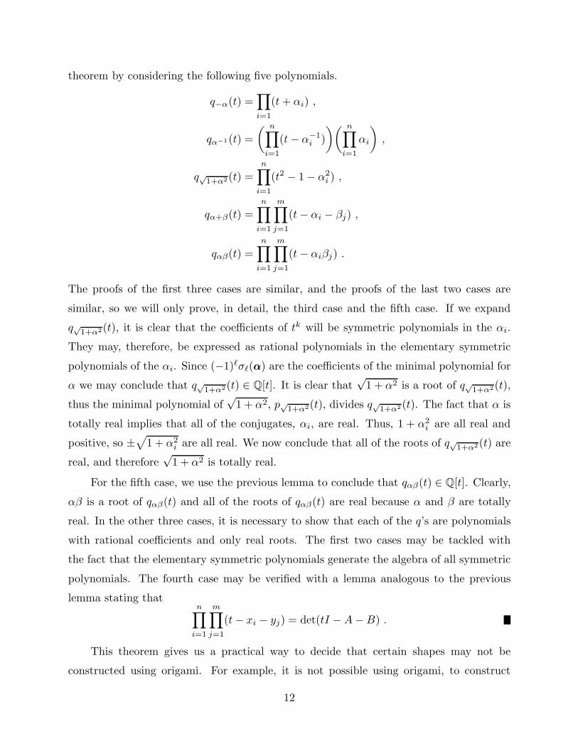
The proofs of the first three cases are similar, and the proofs of the last two cases are

similar, so we will only prove, in detail, the third case and the fifth case. If we expand

q√1+α2(t), it is clear that the coefficients of tk will be symmetric polynomials in the αi.

They may, therefore, be expressed as rational polynomials in the elementary symmetric

polynomials of the αi. Since (−1)ℓσℓ(αα) are the coefficients of the minimal polynomial for

α we may conclude that q√1+α2(t) ∈ Q[t]. It is clear that√

1 + α2 is a root of q√1+α2(t),

thus the minimal polynomial of√

1 + α2, p√1+α2(t), divides q√1+α2(t). The fact that α is

totally real implies that all of the conjugates, αi, are real. Thus, 1 + α2i are all real and

positive, so ±√

1 + α2i are all real. We now conclude that all of the roots of q√1+α2(t) are

real, and therefore√

1 + α2 is totally real.

For the fifth case, we use the previous lemma to conclude that qαβ(t) ∈ Q[t]. Clearly,

αβ is a root of qαβ(t) and all of the roots of qαβ(t) are real because α and β are totally

real. In the other three cases, it is necessary to show that each of the q’s are polynomials

with rational coefficients and only real roots. The first two cases may be tackled with

the fact that the elementary symmetric polynomials generate the algebra of all symmetric

polynomials. The fourth case may be verified with a lemma analogous to the previous

lemma stating thatn

∏

i=1

m∏

j=1

(t − xi − yj) = det(tI − A − B) .

This theorem gives us a practical way to decide that certain shapes may not be

constructed using origami. For example, it is not possible using origami, to construct

12

two cubes such that the volume of the second cube is twice that of the first cube. If this

construction were possible, 3√

2 would be an origami number and would therefore be totally

real. One, however, finds that the conjugates of 3√

2 are 3√

2(−12±

√

32

i) and 3√

2, but the

first two are not real, so 3√

2 is not an origami number.

As we have seen before,√

2 =√

1 + 12 and√

4 + 2√

2 =√

1 + (1 +√

2 )2 are origami

numbers, so√

2 +√

2 =√

2−1√

4 + 2√

2 is an origami number. ¿From this we see the

following corollary.

Corollary. It is not possible to construct a right triangle with arbitrarily given hypotenuse

and leg using origami.

Proof. If this were possible, it would be possible to construct a right triangle with

hypotenuse√

2 +√

2 and leg 1, since these are origami numbers. Any such triangle

would have a leg of length√

1 +√

2 =

√

(√

2 +√

2 )2 − 12, but this is impossible be-

cause√

1 +√

2 is not totally real.

The following corollary is a consequence of the standard algebraic description of com-

pass and straight edge constructions and the two previous theorems [AH].

Corollary. Every thing which is constructible with origami is constructible with a com-

pass and straight edge, but the converse is not true.

We want to expand on the relationship between compass and straight edge construc-

tions and origami constructions. To review, compass and straight edge constructions, let

F√

x be the smallest subfield of C closed under the operation x 7→ √x, then F√

x ∩R is the

collection of numbers which are constructible with a compass and straight edge. ¿From

our work thus far, it is evident that the origami numbers, F0, are contained in F√

x ∩FTR.

It is in fact the case that F0 = F√

x ∩ FTR. This characterization of the origami numbers

is related to David Hilbert’s 17th problem. At the International Congress of Mathematics

at Paris in 1900, Hilbert gave a list of 23 problems [B]. His 17th problem was to show that

any rational function which is non-negative when evaluated at any rational number is a

sum of squares of rational functions. In 1926, Artin solved Hilbert’s 17th problem [Ar].

The key idea which Artin used was the notion of totally positive. An element of a field is

defined to be totally positive if it is positive in every order on the field. Artin proved that

an element is totally positive if and only if it is a sum of squares. This is the idea which

13

we use to prove the final characterization of the origami numbers.

Fact. [L, page 457]. If K is a finite real algebraic extension of Q, then an element of K

is a sum of squares in K if and only if all of its real conjugates are positive.

Theorem. F0 = F√

1+x2 = F√

x ∩ FTR.

Proof. We have already shown that F0 = F√

1+x2 and that F0 ⊂ F√

x ∩ FTR, so we need

to show that F√

x∩FTR ⊂ F√

1+x2 . If α ∈ F√

x∩FTR, then there exists a sequence of totally

real numbers, {βi}ni=1 and a sequence of totally real fields {Kj}n−1

j=0 such that K0 = Q,

Ki = Ki−1(βk), α = βn, and each βi has degree 2 over Ki−1. Since βi has degree 2 over

Ki−1, βi is a root of a polynomial of the form

x2 + cix + di ,

where ci, di ∈ Ki−1. Therefore, (βi + ci/2)2 = c2i /4 − di. By the proof of the previous

theorem, we know that every conjugate of (βi + ci/2)2 is the square of some conjugate of

βi + ci/2. Hence, each of the conjugates of (βi + ci/2)2 are positive and (βi + ci/2)2 is a

sum of squares of elements in Ki−1. Say that

(βi + ci/2)2 = r2i,1 + r2

i,2 + · · ·+ r2i,m ,

then,

βi = ri,1

√

√

√

√

√1 +

ri,2

ri,1

√

1 +

[

ri,3

ri,2

√· · ·

]2

2

− ci

2

and we are done. This shows that any totally real number in F√

x is an origami number.

Legend has it that the ancient Athenians were faced with a plague. In order to remedy

the situation, they sent a delegation to the oracle of Apollo at Delos. This delegation was

told to double the volume of the cubical altar to Apollo. However, the Athenians doubled

the length of each side of the altar, thereby creating an altar with eight times the volume

rather than twice the volume of the original altar. Needless to say, the plague only got

worse. For years, people have tried to double the size of a cube with compass and straight

edge, and the gods have not smiled upon them. We now can see that the gods will not be

satisfied with our elementary origami either.

14

References

[AH] G. Alexanderson, A. Hilman, “A First Undergraduate Course in Abstract Algebra,”3rd edition, Wadsworth Publishing Company, 1983.

[Ar] E. Artin, Uber die zerlegung definiter funktionen in quadrate, Abh. Math. Sem. Hau-sischen Univ. 5 (1927), 100–115.

[B] F. Browder, Mathematical developments arising from Hilbert problems, in “Proceed-ings of Symposia in Pure Mathematics,” Volume 28, American Mathematical Society,1976.

[K] F. Klein, Vortrage uber ausgewahlte Fragen der Elementargeometrie, Teubner, 1895.[L] S. Lang, “Algebra,” 3rd edition, Addison-Wesley, 1993.[M] J. Montroll, “Origami for the Enthusiast,” Dover, 1979.[R] T. Sundara Row, Geometric Exercises in Paper Folding, Dover, 1966.

15