SACLAY–T12/xxx

The Physics of Neutrinos

Renata Zukanovich-Funchal, Benoit Schmauch, Gaëlle Giesen

Abstract

These are the lecture notes of the course given at IPhT.

1

Contents1 Introduction 2

2 Panorama of Experiments 32.1 Early discoveries . . . . . . . . . . . . . . . . . . . . . . . . . . . . . . . . . . . 3

2.1.1 The β-decay problem . . . . . . . . . . . . . . . . . . . . . . . . . . . . . 32.1.2 Discovery of the first neutrino . . . . . . . . . . . . . . . . . . . . . . . . 3

2.2 Towards the Standard Model . . . . . . . . . . . . . . . . . . . . . . . . . . . . . 42.2.1 Discovery of the second neutrino . . . . . . . . . . . . . . . . . . . . . . 42.2.2 Discovery of neutral currents . . . . . . . . . . . . . . . . . . . . . . . . . 5

2.3 The quest for neutrino oscillations . . . . . . . . . . . . . . . . . . . . . . . . . . 62.3.1 Atmospheric neutrinos (Eν ∼ (10−1 − 103) GeV) . . . . . . . . . . . . . . 72.3.2 Accelerator neutrinos (Eν ∼ (1− 10) GeV) . . . . . . . . . . . . . . . . . 112.3.3 Solar neutrinos (Eν ∼ (0.1− 10) MeV) . . . . . . . . . . . . . . . . . . . 112.3.4 Reactor neutrinos (Eν ∼ (1− 10) MeV) . . . . . . . . . . . . . . . . . . . 12

2.4 First hints of a new mixing . . . . . . . . . . . . . . . . . . . . . . . . . . . . . . 132.5 Other properties of neutrinos . . . . . . . . . . . . . . . . . . . . . . . . . . . . 13

2.5.1 Anomalies . . . . . . . . . . . . . . . . . . . . . . . . . . . . . . . . . . . 132.5.2 Limits on Neutrino masses . . . . . . . . . . . . . . . . . . . . . . . . . . 132.5.3 Are ν 6= ν? . . . . . . . . . . . . . . . . . . . . . . . . . . . . . . . . . . 14

1 Introduction"Some scientific revolutions arise from the invention of new tools or techniques for observingnature; others arise from the from the discovery of new concepts for understanding nature [..]The progress of science requires both new concepts and new tools". These two quotes of FreemanDyson illustrate perfectly the research in neutrino physics. On one hand the theoretical workneeds revolution and invention. On the other hand, the experimental approach towards thisfield is extremely complicated and has to overcome the difficulties due to the very small massand interaction probability of neutrinos. The discovery of neutrinos and posteriors of neutrinooscillations needed the device of new tools and experimental techniques.Neutrino sources can be man made, such as nuclear reactors or accelerators, but are alsoproduced by the atmosphere, the earth, the sun or are part of the relic from the Big Bang.To have a quantitative understanding of neutrinos, let us start with some numbers: our bodyemits 350 million neutrinos a day, receives from the sun 400 trillion/s, the earth 50 billion/sand nuclear reactors around 10-100 billion/s.

2

2 Panorama of Experiments

2.1 Early discoveries2.1.1 The β-decay problem

The first evidence for the existence of neutrinos appeared in 1899, when Ernest Rutherforddiscovered β− decay, in which a nucleus with electric charge Z decays into another one withcharge Z + 1 and an electron, i.e.

A(N,Z)→ A′(N − 1, Z + 1) + e−.

This reaction was first thought of as a two-body decay, and so the emitted electron was expectedto be monochromatic, but between 1920 and 1927 Charles Drummond Ellis, along with JamesChadwick, proved that it had a continuous energy spectrum. This result seemed to be incontradiction with the conservation of energy, until Wolfgang Pauli made the hypothesis that aneutral particle with spin 1/2 was emitted together with the electron in β− decays (1930). Hecalled this particle neutron, and established that its mass should not be larger than 0.01 protonmass. In 1932, James Chadwick discovered the neutron, whose mass was of the same order ofmagnitude as that of the proton (so it couldn’t be Pauli’s particle). In 1934, β+ radioactivitywas discovered by Frédéric and Irène Joliot-Curie. The same year, Fermi proposed his theoryfor the weak interaction to explain β radioactivity and renamed Pauli’s particle neutrino.In Fermi’s theory, weak interaction was described as a four-fermion interaction, driven by theeffective lagrangian

LFermi = GF√2

(ΨpγµΨn)(ΨeγµΨν). (2.1)

According to Fermi’s theory, the cross-section for the scattering of a neutrino with a neutronwas

σ(ne + ν → e− + p) ∼ Eν(MeV)× 1043 cm2. (2.2)

This result means that 50 light-years of water would be necessary to stop a 1 MeV neutrino,which seems to make the experimental observation of these particles a hopeless task. But,as explained in the introduction, neutrinos are everywhere, and this ubiquity permitted theirdetection.In particular, the invention of nuclear reactor and particle accelerators in the 50’sfacilitated the endeavor.

2.1.2 Discovery of the first neutrino

In 1956, more than 20 years after Fermi proposed his theory, the first neutrino, now known asthe electron neutrino, was detected by Fred Reines and Clyde Cowan (actually, since we don’tknow yet whether neutrinos are their own antiparticles or not, the particle discovered by Reinesand Cowan should rather be called an antineutrino), thanks to a liquid scintillator detector, in

3

which antineutrinos undergo the so-called inverse β decay and are captured by protons in thetarget as

νe + p→ e+ + n.

The positron annihilates immediately with an electron into two photons. After a flight time of207 µs, the emitted neutron combines with a proton to form a deuterium nucleus, and a photonwith energy 2.2 MeV is emitted in the process

n+ p→ d+ γ.

The combination of these two events is interpreted as the signal of an antineutrino.

2.2 Towards the Standard Model2.2.1 Discovery of the second neutrino

The second type of neutrino was discovered six years later by Jack Steinberger, Leon Ledermanand Melvin Schwartz. This new neutrino was found to appear in interactions involving muonsand was consequently named muon neutrino. In this experiment, pions produced in proton-proton collisions decayed into muons and muon neutrinos

p+ p→ π + hadrons,

π → µ+ νµ.

The muon neutrinos were detected in a spark chamber, thanks to the reaction

νµ +N → µ+ hadrons,

where N is a nucleon. Short after it was shown that reactions involving neutrinos violate parityP and charge conjugation C but conserve CP . Let us define here some notions: helicity h isdefined as the projection of the spin onto the direction of the momentum

h = ~σ.~p

|~p|, (2.3)

whereas chirality is a more abstract notion, which is determined by how the spinor transformsunder the Poincaré group. One can define the projector onto the positive and negative helicitystates as

P± = 12

(1± ~σ.~p

|~p|

)' PR/L +O(m

E), (2.4)

where PR and PL are the projectors onto the right-handed and left-handed chirality states,defined as

PR/L = 12(1± γ5) (2.5)

4

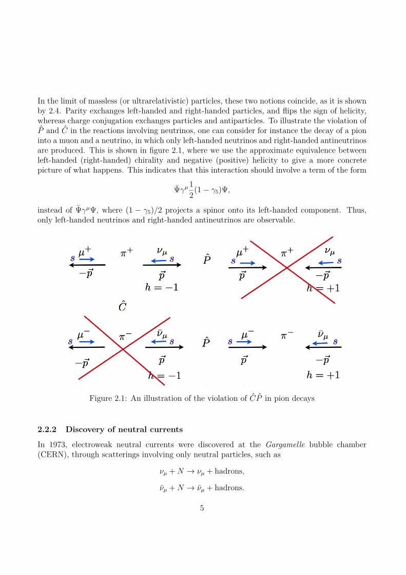
In the limit of massless (or ultrarelativistic) particles, these two notions coincide, as it is shownby 2.4. Parity exchanges left-handed and right-handed particles, and flips the sign of helicity,whereas charge conjugation exchanges particles and antiparticles. To illustrate the violation ofP and C in the reactions involving neutrinos, one can consider for instance the decay of a pioninto a muon and a neutrino, in which only left-handed neutrinos and right-handed antineutrinosare produced. This is shown in figure 2.1, where we use the approximate equivalence betweenleft-handed (right-handed) chirality and negative (positive) helicity to give a more concretepicture of what happens. This indicates that this interaction should involve a term of the form

Ψγµ12(1− γ5)Ψ,

instead of ΨγµΨ, where (1 − γ5)/2 projects a spinor onto its left-handed component. Thus,only left-handed neutrinos and right-handed antineutrinos are observable.

Figure 2.1: An illustration of the violation of CP in pion decays

2.2.2 Discovery of neutral currents

In 1973, electroweak neutral currents were discovered at the Gargamelle bubble chamber(CERN), through scatterings involving only neutral particles, such as

νµ +N → νµ + hadrons,

νµ +N → νµ + hadrons.

5

This was a first confirmation of the validity of the model proposed by Abdus Salam, SheldonGlashow and Steven Weinberg for the electroweak interaction. As it is now well-known, left-handed (right-handed) (anti-)quarks and (anti-)leptons fall into doublets, each doublet beingcharacterized by its flavor. Each lepton doublet contains a particle with charge -1 and aneutrino. The lagrangian of this model contains the following terms, accounting for the chargedcurrent (cc) and neutral current (nc) interactions respectively:

L = − g√2jµccWµ −

g

cos θWjµncZµ + h.c. (2.6)

The charged and neutral current are

jµcc = fαγµPLf

′α, (2.7)

jµnc = fαγµPLfα, (2.8)

where α stands for the flavor.According to the LEP experiments which measured the invisible decay width of the Z0 bosonproduced in electron-positron collisions, there should exist three types of light neutrinos (witha mass less or equal to mZ/2) that couple to the Z0 lepton in the usual way (more precisely theresult of these combined experiments gives Nν = 2.984 ± 0.008). This was confirmed in 2000by the discovery of the third neutrino, associated with the tau, by the DONUT collaborationat Fermilab.

2.3 The quest for neutrino oscillationsIn the 1960’s, Kaon oscillations had already been discovered, which motivated the idea thatneutrino may oscillate too, even though this is not predicted by the standard model.To measure the oscillations of neutrinos, there are two types of experiments that one can do:

• The disappearance experiments are historically the first ones built and concludingtowards neutrino oscillations. The basic concept is the following: a source produces aknown (either through theoretical models of natural sources or through man made andcontrolled production) amount of (anti-)neutrinos of flavor α. At a distance L, the numberof detected neutrinos of flavor α in the experiment is then

Nα(L) = A∫

Φ(E)σ(E)P (να → να;E,L)ε(E), (2.9)

with A the number of targets multiplied by the time of exposure, Φ(E) the ν flux, P (να →να;E,L) the survival probability and ε(E) the detector efficiency.

• In the appearance experiments, one considers again a source of neutrinos of flavor α,but then one detects neutrinos of a different flavor β (α 6= β).

6

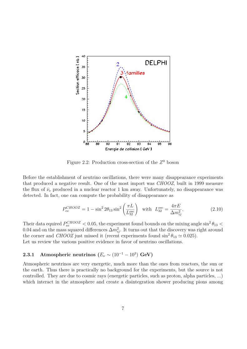
Figure 2.2: Production cross-section of the Z0 boson

Before the establishment of neutrino oscillations, there were many disappearance experimentsthat produced a negative result. One of the most import was CHOOZ, built in 1999 measurethe flux of νe produced in a nuclear reactor 1 km away. Unfortunately, no disappearance wasdetected. In fact, one can compute the probability of disappearance as

PCHOOZee = 1− sin2 2θ13 sin2

(πL

Losc32

)with Losc32 = 4πE

∆m2ij

. (2.10)

Their data equired PCHOOZee < 0.05, the experiment found bounds on the mixing angle sin2 θ13 <

0.04 and on the mass squared differences ∆m2ij. It turns out that the discovery was right around

the corner and CHOOZ just missed it (recent experiments found sin2 θ13 ' 0.025).Let us review the various positive evidence in favor of neutrino oscillations.

2.3.1 Atmospheric neutrinos (Eν ∼ (10−1 − 103) GeV)

Atmospheric neutrinos are very energetic, much more than the ones from reactors, the sun orthe earth. Thus there is practically no background for the experiments, but the source is notcontrolled. They are due to cosmic rays (energetic particles, such as proton, alpha particles, ...)which interact in the atmosphere and create a disintegration shower producing pions among

7

others. These pions then decay into

π+ → µ+ + νµ and then µ+ → e+ + νe + νµ,

π− → µ− + νµ and then µ− → e− + νe + νµ.

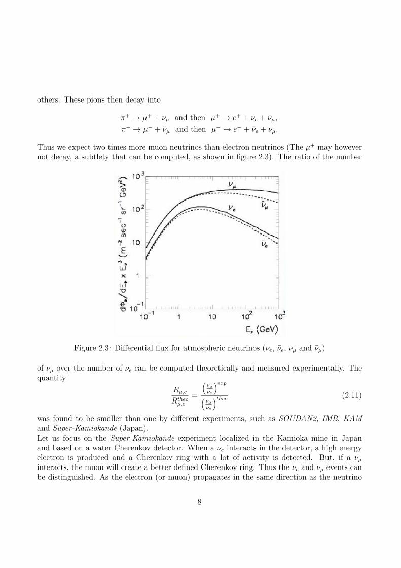
Thus we expect two times more muon neutrinos than electron neutrinos (The µ+ may howevernot decay, a subtlety that can be computed, as shown in figure 2.3). The ratio of the number

Figure 2.3: Differential flux for atmospheric neutrinos (νe, νe, νµ and νµ)

of νµ over the number of νe can be computed theoretically and measured experimentally. Thequantity

Rµ,e

Rtheoµ,e

=

(νµνe

)exp(νµνe

)theo (2.11)

was found to be smaller than one by different experiments, such as SOUDAN2, IMB, KAMand Super-Kamiokande (Japan).Let us focus on the Super-Kamiokande experiment localized in the Kamioka mine in Japanand based on a water Cherenkov detector. When a νe interacts in the detector, a high energyelectron is produced and a Cherenkov ring with a lot of activity is detected. But, if a νµinteracts, the muon will create a better defined Cherenkov ring. Thus the νe and νµ events canbe distinguished. As the electron (or muon) propagates in the same direction as the neutrino

8

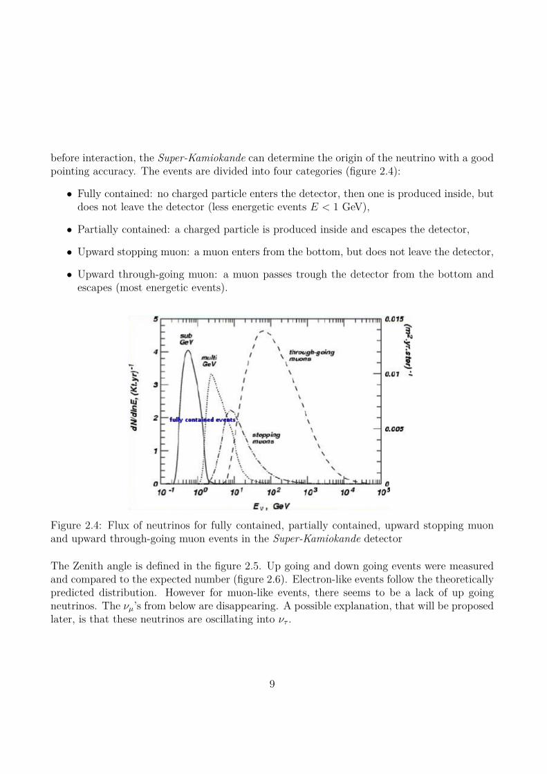
before interaction, the Super-Kamiokande can determine the origin of the neutrino with a goodpointing accuracy. The events are divided into four categories (figure 2.4):

• Fully contained: no charged particle enters the detector, then one is produced inside, butdoes not leave the detector (less energetic events E < 1 GeV),

• Partially contained: a charged particle is produced inside and escapes the detector,

• Upward stopping muon: a muon enters from the bottom, but does not leave the detector,

• Upward through-going muon: a muon passes trough the detector from the bottom andescapes (most energetic events).

Figure 2.4: Flux of neutrinos for fully contained, partially contained, upward stopping muonand upward through-going muon events in the Super-Kamiokande detector

The Zenith angle is defined in the figure 2.5. Up going and down going events were measuredand compared to the expected number (figure 2.6). Electron-like events follow the theoreticallypredicted distribution. However for muon-like events, there seems to be a lack of up goingneutrinos. The νµ’s from below are disappearing. A possible explanation, that will be proposedlater, is that these neutrinos are oscillating into ντ .

9

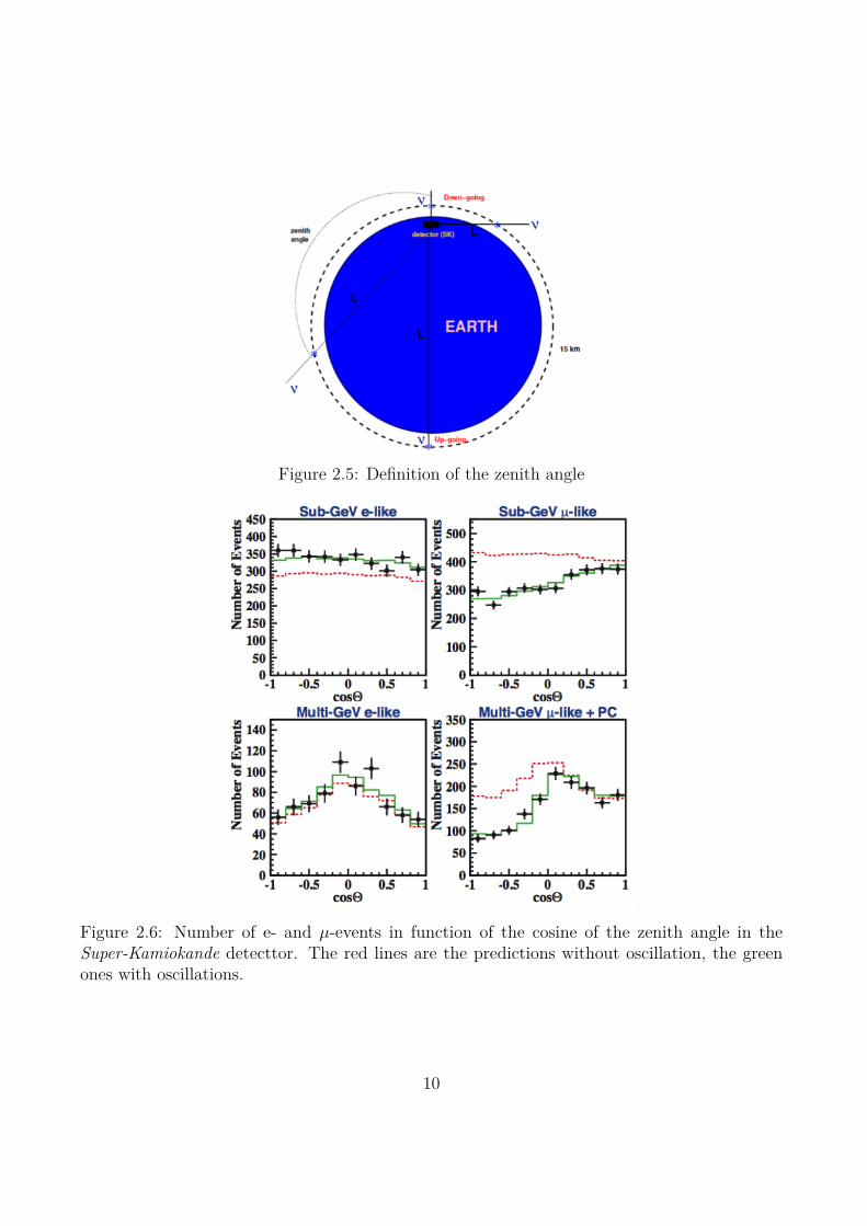
Figure 2.5: Definition of the zenith angle

Figure 2.6: Number of e- and µ-events in function of the cosine of the zenith angle in theSuper-Kamiokande detecttor. The red lines are the predictions without oscillation, the greenones with oscillations.

10

2.3.2 Accelerator neutrinos (Eν ∼ (1− 10) GeV)

In particle accelerators, the production of pions is well controlled. These pions decay throughthe same process as described above into a well known number of neutrinos. The experimentsK2K (Japan) and MINOS (USA) tried to measure the disappearance of νµ. The data of K2Kgives some evidence in this direction but is less conclusive. But in the MINOS experimentneutrinos were definitely missing, thus confirming the results from Super-Kamiokande.

2.3.3 Solar neutrinos (Eν ∼ (0.1− 10) MeV)

In the sun, nuclear fusion produces electron neutrinos νe through the pp-cycle

41H → 4He+ 2e+ + 2νe + energy

or through CNO-cycle (Carbon, Nitrogen, Oxygen), for example. Only electron neutrinos areproduced by the sun, at its center (at a radius < 0.3 R) and they only need 9 minutes toarrive on earth (photons need millions of years to reach the photosphere). pp-neutrinos arevery abundant, but have low energy, whereas B-neutrinos (B for Bore) are very energetic butrare. Experiments on earth tried to measure these solar neutrinos:

• The Homestake (USA) experiment used a tank of liquid chlorine C2Cl4. If a neutrinointeracts inside, an inverse β-decay will take place

νe + 37Cl→ e− + 37Ar at Eth = 814 keV.

Thus the number of argon atoms is equal to the number of interacting neutrinos. Throughthe whole duration of the experiment (1968-94), the number of observed events was 1/3smaller than what was expected. Nevertheless, at that time, the credibility of these resultswas questioned because of the complexity of the setup.

• Gallium experiments (for example in Gran Sasso) take also advantage of the inverse β-decay with the reaction

νe + 71Ga→ e− + 71Ge at Eth = 233 keV.

This is also a radio chemical experiment that measures νe by charged current interaction.They have measured about 60 % of the events expected.For the measurements of these solar neutrinos a new unit is introduced: SNU (StandardSolar Unit) which corresponds to the number of interactions per 1036 atoms per second.

• The Super-Kamionande, described above, can also detect solar neutrinos, by measuringthe elastic scattering of a neutrino on an electron of a water molecule,

νx + e− → νx + e− with x = e, µ at Eth = 5 MeV.

11

As this experiment is able to point at the neutrino source, the detector took the first"neutrinography" of the sun. It measures about 45 % of neutrinos expected.The SNO experiment is also a Cherenkov detector, but using heavy water. Thus, reactionswith deuterium are observed:

νx + e− → νx + e− CC and NCνe + d→ e− + p+ p, CCνx + d→ νx + p+ n NC.

So they measured νe as well as all other flavors of neutrinos through the NC reaction.

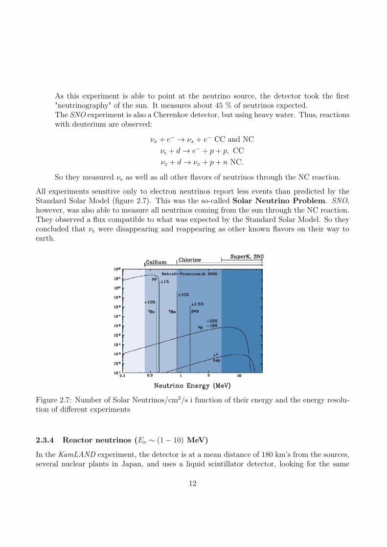
All experiments sensitive only to electron neutrinos report less events than predicted by theStandard Solar Model (figure 2.7). This was the so-called Solar Neutrino Problem. SNO,however, was also able to measure all neutrinos coming from the sun through the NC reaction.They observed a flux compatible to what was expected by the Standard Solar Model. So theyconcluded that νe were disappearing and reappearing as other known flavors on their way toearth.

Figure 2.7: Number of Solar Neutrinos/cm2/s i function of their energy and the energy resolu-tion of different experiments

2.3.4 Reactor neutrinos (Eν ∼ (1− 10) MeV)

In the KamLAND experiment, the detector is at a mean distance of 180 km’s from the sources,several nuclear plants in Japan, and uses a liquid scintillator detector, looking for the same

12

inverse β+ decay than Raines and Cowan in 1956. It confirmed the results obtained with solarneutrinos for the first time and pinned down the solution for the solar neutrino problem as thelarge mixing angle one.

2.4 First hints of a new mixingThe first appearance of νe (νµ → νe) was measured by T2K in June 2011. In fact, 1.5 νe-eventswere expected and 6 were observed, which is consistent with MINOS and was confirmed byDouble CHOOZ in the end of 2011 and Daya Bay in march 2012, both studying νe → νe.

2.5 Other properties of neutrinos2.5.1 Anomalies

Several experiments show anomalies and intriguing results, maybe pointing toward a morecomplex theory of neutrino physics:

• Gallium anomaly: the detectors using Gallium are calibrated with radioactive sources,but the data and the theoretical predictions seem to be at odds,

• LSND/miniBooNE anomaly: both experiments study νµ → νe and see appearance thatcannot satisfactorily be explained. In particular, there seems to be some tension betweenthe results and the other neutrino oscillation experiments.

• Reactor anomaly: after a recalculation of the νe flux from reactors, it was shown thatall short baseline (L . 100 m) experiments measuring reactor neutrinos seem to havemesured less events than expected.

2.5.2 Limits on Neutrino masses

As we will see shortly, the simplest framework that can account for neutrino oscilations relieson neutrinos having mass. Different ways of constraining their mass exist, we present two ofthem:

• Tritium β-decay: The reaction considered is 3H →3 He+ e− + νe with an energy releaseQ = MH − MHe − me = 18.58 keV. The differential decay rate of the isotope can bewritten as

dΓdT∝ |M|2 F (E)pE(Q− T )

√(Q− T )2 −m2

νe ,

where T , p and E are respectively the kinetic energy, the momentum and the total energyof the electron. F (E) is the Fermi function which accounts for the influence of the nucleon

13

Coulomb field, |M|2 the squared matrix element and mνe is the effective νe mass.One can draw a Kurie plot, i.e. the function

K(T ) =√

(Q− T )√

(Q− T )2 −m2νe .

Troisk and Mainz found in 2002 the limit mνe < 2.2 eV. The future experiment KATRINshould have a sensitivity down to 0.2 eV.

• Relic neutrinos: The cosmic microwave background (CMB) can give information on thesum of all the neutrino masses. In fact the neutrino abundance can be measured andeasily be related to the masses in the following way,

Ωνh2 =

∑k

nνkmk

ρc=

∑kmk

94.14eV .

The 9 year data of WMAP gives ∑kmk < 0.44 eV at 95% C.L.

2.5.3 Are ν 6= ν?

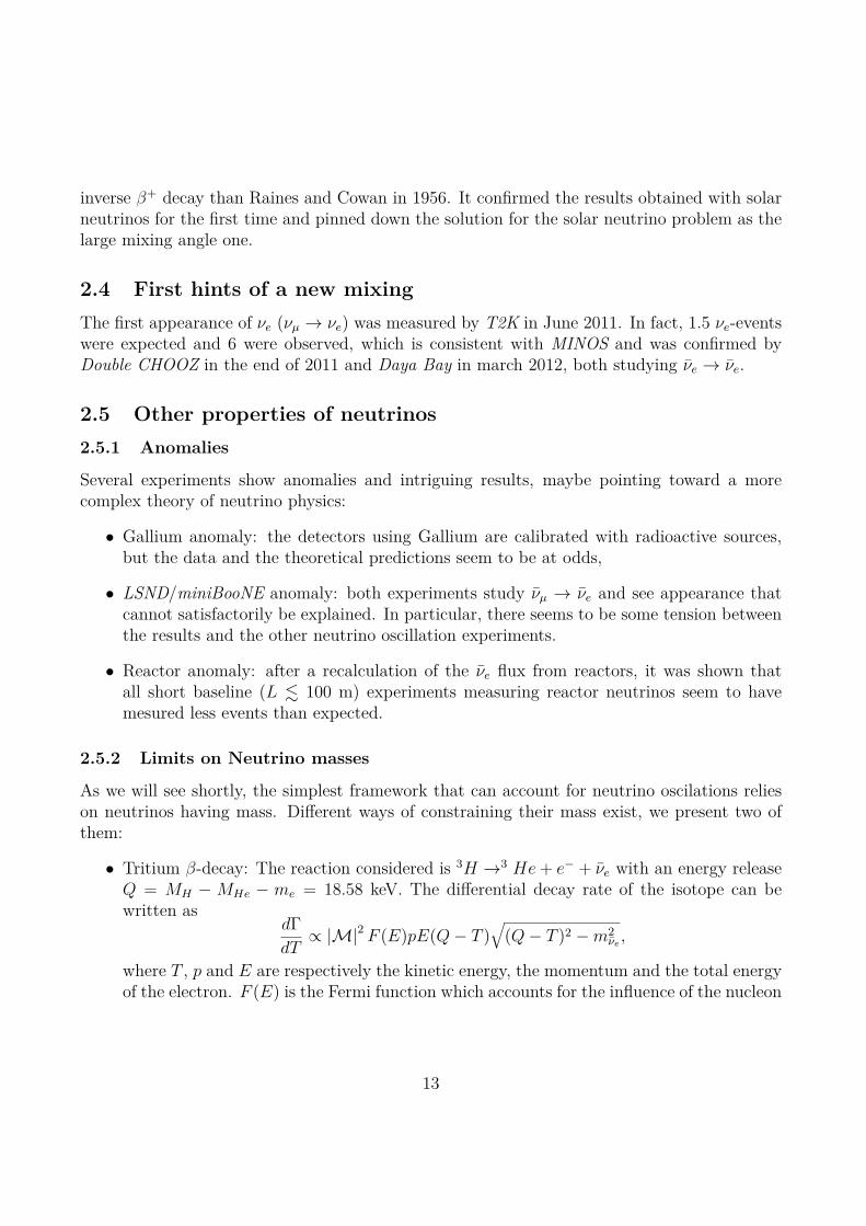
All the fermions known today are Dirac fermions, i.e. f 6= f . Neutrinos could perhaps be Ma-jorana fermions, ν = ν. A signature of this property would be the existence of the neutrinolessdouble β-decay. The only reaction allowed if neutrinos were Dirac fermions would be the twoneutrino double β-decay

N(A,Z)→ N(A,Z + 2) + e− + e− + νe + νe.

The lepton number is conserved in this second order weak interaction process (∆L = 0) and

the half-life decay of the isotope T 2ν12

can be written as (T 2ν12

)−1 = G2ν |M2ν |2, where G2ν is a

14

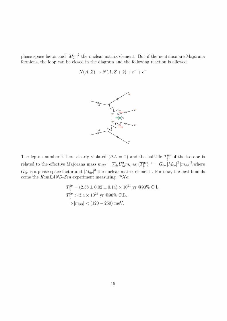
phase space factor and |M2ν |2 the nuclear matrix element. But if the neutrinos are Majoranafermions, the loop can be closed in the diagram and the following reaction is allowed

N(A,Z)→ N(A,Z + 2) + e− + e−

The lepton number is here clearly violated (∆L = 2) and the half-life T 0ν12

of the isotope isrelated to the effective Majorana mass mββ = ∑

k U2ekmk as (T 0ν

12

)−1 = G0ν |M0ν |2 |mββ|2,whereG0ν is a phase space factor and |M0ν |2 the nuclear matrix element . For now, the best boundscome the KamLAND-Zen experiment measuring 136Xe:

T 2ν12

= (2.38± 0.02± 0.14)× 1021 yr @90% C.L.

T 0ν12> 3.4× 1025 yr @90% C.L.

⇒|mββ| < (120− 250) meV.

15