Theoretical Background for the Inversion of Seismic ...
35
Theoretical Background for the Inversion of Seismic Waveforms, Including Elasticity and Attenuation Albert Tarantola Institut de Physique du Globe, 4 place Jussieu, 75005 Paris, France. Pure and Applied Geophysics, Vol. 128, Nos. 1/2, 1988, p. 365–399 Abstract —To account for elastic and attenuating effects in the elastic wave equation, the stress-strain relationship can be defined through a general, anisotropic, causal relaxation func- tion ψ ijkl (x,τ ). Then, the wave equation operator is not necessarily symmetric (‘self-adjoint’), but the reciprocity property is still satisfied. The representation theorem contains a term pro- portional to the history of strain. The dual problem consists of solving the wave equation with final time conditions and an anti-causal relaxation function. The problem of interpretation of seismic waveforms can be set as the nonlinear inverse problem of estimating the matter density ρ(x) and all the functions ψ ijkl (x,τ ). This inverse problem can be solved using itera- tive gradient methods, each iteration consisting of the propagation of the actual source in the current medium, with causal attenuation, the propagation of the residuals—acting as if they were sources— backwards in time, with anti-causal attenuation, and the correlation of the two wavefields thus obtained. Key words: Inversion, waveforms, attenuation, Green’s function, representation theorem, dual conditions, reciprocity theorem. 1. Introduction The problem of interpretation of seismic waveforms can be set as the problem of obtaining the earth model which best predicts the actually observed seismograms. This opens two questions: (i) given an earth model, how to solve the forward problem of predicting seismograms? and (ii) how to solve the inverse problem of obtaining the optimum earth model? The tools for predicting seismograms are the elastic wave equation and the numerical meth- ods developed to obtain solutions, as for instance finite-difference approximations to derivatives. Finite-difference approximations to the wave equation have the advantages of having enough flexibility to be almost model-independent and of accounting, in principle, for a diversity of waves. They are expensive, but nicely adaptable to the newly emerging class of massively parallel computers. 365
Transcript of Theoretical Background for the Inversion of Seismic ...
Theoretical Background for the Inversionof Seismic Waveforms,
Including Elasticity and Attenuation
Albert Tarantola
Institut de Physique du Globe, 4 place Jussieu, 75005 Paris, France.
Pure and Applied Geophysics, Vol. 128, Nos. 1/2, 1988, p. 365–399
Abstract—To account for elastic and attenuating effects in the elastic wave equation, thestress-strain relationship can be defined through a general, anisotropic, causal relaxation func-tion ψijkl(x, τ). Then, the wave equation operator is not necessarily symmetric (‘self-adjoint’),but the reciprocity property is still satisfied. The representation theorem contains a term pro-portional to the history of strain. The dual problem consists of solving the wave equation withfinal time conditions and an anti-causal relaxation function. The problem of interpretationof seismic waveforms can be set as the nonlinear inverse problem of estimating the matterdensity ρ(x) and all the functions ψijkl(x, τ). This inverse problem can be solved using itera-tive gradient methods, each iteration consisting of the propagation of the actual source in thecurrent medium, with causal attenuation, the propagation of the residuals—acting as if theywere sources— backwards in time, with anti-causal attenuation, and the correlation of the twowavefields thus obtained.
Key words: Inversion, waveforms, attenuation, Green’s function, representation theorem,dual conditions, reciprocity theorem.
1. Introduction
The problem of interpretation of seismic waveforms can be set as the problem of obtaining theearth model which best predicts the actually observed seismograms. This opens two questions:(i) given an earth model, how to solve the forward problem of predicting seismograms? and (ii)how to solve the inverse problem of obtaining the optimum earth model?
The tools for predicting seismograms are the elastic wave equation and the numerical meth-ods developed to obtain solutions, as for instance finite-difference approximations to derivatives.Finite-difference approximations to the wave equation have the advantages of having enoughflexibility to be almost model-independent and of accounting, in principle, for a diversity ofwaves. They are expensive, but nicely adaptable to the newly emerging class of massivelyparallel computers.
365
366 Albert Tarantola: Background for the Inversion of Seismic Waveforms
The inverse problem is essentially an optimization problem in a functional space. Difficultiesarise because the problem is large sized, and the functional to be minimized is nonquadratic.The modest capabilities of present-day computers prevent the use of true nonquadratic methodsof optimization, like Monte Carlo methods. Gradient methods can be used which lead to elegantresults.
In this paper I first review the mathematics of the forward problem that are useful for theinverse problem; wave equation, Green’s function, and representation theorem. Secondly, Ireview the mathematics of functional least squares. Finally, I give the solution to the seismicinverse problem, with more generality than in my previous papers, because here I take intoaccount attenuation.
In the problem of interpretation of seismic reflection data the model space has many degreesof freedom (millions to billions), and methods of inversion based on a naıve use of least-squaresformulas do not work. In particular, matrix algebra must not be used, and partial (or Frechet)derivatives of data with respect to model parameters should not be computed. Much work hasto be done analytically, in order to interpret the final formulas of least squares as operationsinvolving only wave propagations, and no linear algebra computations.
For developing a theory for inversion including attenuation we must first choose a model.If in the perfectly elastic approximation it is clear that density ρ(x) and elastic stiffnessescijkl(x) (or related quantities) are the right earth parameters to choose, for a more realistic ap-proximation including attenuation, the choice is not so clear, as many models for attenuationexist. I take here the most optimistic point of view: that data sets exist which contain enoughinformation rendering a particular model of attenuation unnecessary, and that the more gen-eral parameterization can be chosen: an arbitrary relaxation function ψijkl(x, τ). The goal ofinversion is then to obtain the density ρ(x) and the functions ψijkl(x, τ). Of course, some con-straints have to be imposed on the relaxation functions, as for instance causality and symmetryconditions. If necessary, some soft constraints can also be imposed, as for instance spatial ortemporal smoothness.
Let ui(x, t) be the i-th component of displacement at point x and time t. If xr (r = 1, 2, . . .)denote the receiver locations, a possible criterion of goodness of fit between observed andcomputed seismograms is the minimization of
S =∑
r
∫ t1
t0
dt∑
i
∣∣∣ui(xr, t
)obs−
(xr, t
)cal
∣∣∣, (1a)
where ‘obs’ and ‘cal’ respectively represent the observed and the calculated displacements froma given earth model. Although results given by this criterion are fairly good, they are difficultto obtain, and this criterion is replaced by the least-squares criterion of minimization of
S =∑
r
∫ t1
t0
dt∑
i
(ui
(xr, t
)obs− ui
(xr, t
)cal
)2
, (1b)
which gives less robust results but computations which are manageable with present: daycomputers.
PAGEOPH, Vol. 128, Nos. 1/2, 1988, p. 365–399 367
In Section 2 the rate-of-relaxation function is defined, which will be at the center of ourmathematical developments. Section 3 rapidly reviews the fundamental equation: the elasticwave equation with attenuation. In Section 4 I recall the definition of the transposed (andadjoint) of an operator, and in Section 5 the transposed of the wave equation operator is given.The Green function is introduced in Section 6, leading to the general representation theoremsof Section 7, which are independent of the reciprocity relations shown in Section 8. Section9 reviews rapidly the Born approximation, useful for computing the gradient of the least-squares misfit function. A very formal version of the least-squares theory in functional spacesis developed in Section 10, and is applied to the problem of interpretation of seismic waveformsin Section 11. The formula allowing waveform inversion for obtaining the rate-of-relaxationfunction is, to my knowledge, original. The last Section addresses the results obtained.
2. The Rate-of-Relaxation Function
The most general linear relationship between stress, σij(x, t), and strain εij(x, t), can be de-scribed using a kernel Ψijkl
1 (x, t;x′, t′):
σij(x, t) =
∫V
dV (x′)
∫ +∞
−∞dt′Ψijkl
1 (x, t;x′, t′)εkl(x′, t′), (2a)
which has to be causal, must have some symmetries, and may be a distribution (containing thedelta ‘function’ and/or its derivatives). This is too general for most seismic purposes. Assumingthat the stress-strain relationship is local,
Ψijkl1 (x, t;x′, t′) = Ψijkl
0 (x; t, t′)δ(x− x′),
gives
σij(x, t) =
∫ +∞
−∞dt′Ψijkl
0 (x; t, t′)εkl(x, t′). (2b)
If the medium properties do not depend on time,
Ψijkl0 (x; t, t′) = Ψijkl(x, t− t′),
and
σij(x, t) =
∫ +∞
−∞dt′Ψijkl(x, t− t′)εkl(x, t′). (2c)
The function Ψijkl(x, τ) has to satisfy causality,
Ψijkl(x, τ) = 0 for τ < 0, (3)
and is assumed to have symmetries:
Ψijkl(x, τ) = Ψjikl(x, τ) = Ψklij(x, τ), (4)
368 Albert Tarantola: Background for the Inversion of Seismic Waveforms
(from where it follows Ψijkl(x, τ) = Ψijlk(x, τ) = Ψjikl(x, τ)). Notice that the causality propertyallows writing (2c) as
σij(x, t) =
∫ t+
−∞dt′Ψijkl(x, t− t′)εkl(x, t′).
Instead of the function Ψijkl(x, τ) it is customary to use the creep function φijkl(x, τ) definedby
εij(x, t) =
∫ t
−∞dt′φijkl(x, t− t′)σkl(x, t′), (5)
or its inverse, the relaxation function ψijkl(x, τ) defined by
σij(x, t) =
∫ t
−∞dt′ψijkl(x, t− t′)εkl(x, t′), (6)
where a dot denotes time differentiation. As we have
Ψijkl(x, τ) = ψijkl(x, τ), (7)
Ψijkl(x, τ) can be named the rate-of-relaxation function.
Example 1. Perfect elasticity. Choosing
Ψijkl(x, τ) = cijkl(x)δ(τ), (8)
where δ(·) is the delta ‘function’, gives Hooke’s law
σij(x, t) = cijkl(x)εkl(x, t). (9)
For isotropic media,cijkl(x) = λe(x)δijδkl + µe(x)
(δikδjl + δilδjk
), (10)
where λe(x) and µe(x) are the (elastic) parameters of Lame, related with the elastic bulkmodulus by
3ke(x) = 3λe(x) + 2µe(x). (11)
As a first approximation, for usual rocks, λe ' µe.
Example 2. Elasticity with viscosity. Choosing
Ψijkl(x, τ) = cijkl(x)δ(τ)− dijkl(x)δ(τ), (12)
gives the Kelvin-Voigt law
σij(x, t) = cijkl(x)εkl(x, t) + dijkl(x)εkl(x, t), (13)
which corresponds, in a 1D problem, to a perfectly elastic spring and a perfectly viscous dashpotin parallel. For isotropic viscosity,
dijkl(x) = λv(x)δijδkl + µv(x)(δikδjl + δilδjk
). (14)
The viscous bulk modulus is defined by
3kv(x) = 3λv(x) + 2µv(x). (15)
As a first approximation, for usual rocks, 3kv = 3λv + 2µv ' 0.
PAGEOPH, Vol. 128, Nos. 1/2, 1988, p. 365–399 369
Example 3. Constant Q. In a one-dimensional example, KJARTANSSON (1979) shows thatthe rate-of-relaxation function
Ψ(τ) ∝ 1
τ 1+2γfor τ > 0 (16)
Ψ(τ) = 0 for τ ≤ 0 (17)
implies a quality factor Q strictly independent on the frequency, and, for a sufficiently smallvalue of the positive parameter γ, fits most of seismic data.
3. The Fundamental Equation
Let us be interested in the description of elastic waves propagating inside a volume V, sur-rounded by a surface S. Points inside V will be denoted x,x′, . . . while points on S will bedenoted ξ, ξ′, . . .. From the fundamental laws of physics we can show (e.g., DAUTRAY andLIONS, 1984) that if we impose to a medium with matter density ρ(x) and rate-of-relaxationfunction Ψijkl(x, τ), a volume density of force φi(x, t), a moment density M ij(x, t), and a sur-face traction τ i(ξ, τ), then the displacement field ui(x, t) satisfies at any point inside V therelationship
ρ(x)∂2ui
∂t2(x, t)− ∂σij
∂xj(x, t) = φi(x, t) (18)
where
σij(x, t) = M ij(x, t) +
∫ +∞
−∞dt′Ψijkl(x, t− t′)∂u
k
∂xl(x, t′), (19)
and, at the surface,
nj(ξ)σij(ξ, t) = τ i(ξ, t). (20)
Notice that σij(x, t) is the total stress (internal plus external origin) and that in the equationsof the previous section the external stress M ij(x, t) was implicitly assumed to be zero.
4. Mathematical Preliminary: Symmetric and Self-Adjoint Operators
Let U be a linear space, whose elements, denoted u, are named vectors. For instance eachelement of U may be a displacement field ui(x, t). A Linear form over U is a linear applicationfrom U into a space of scalars (identical to the real numbers of R excepted in that the scalarsmay have a physical dimension). We will say that a linear space U is a dual of U if eachelement of U defines a linear form over U (I prefer that definition to the traditional definitionof mathematicians where the dual is the space of all linear forms). Let u0 ∈ U. The scalarassociated to any u ∈ U by u0 is denoted by 〈u0,u〉U . Alternatively, each element u0 ∈ Udefines a linear form over U through⟨
u0, u⟩
U=
⟨u,u0
⟩U. (21)
370 Albert Tarantola: Background for the Inversion of Seismic Waveforms
Let U and Φ be two linear spaces, and L a linear operator from U into Φ. For instance, Lmay be the wave equation operator defined in Section 5. An operator Lt mapping Φ into Uwill be named the transposed of L if for any φ ∈ Φ and any u ∈ U⟨
φ,Lu⟩
Φ=
⟨Ltφ,u
⟩U. (22)
This definition of transposed operators may be compared with the definition of adjointoperators. The adjoint of an operator may only be defined if the spaces in consideration havea scalar product. Let for instance the linear operator L map the linear space U into the linearspace Φ, and let (u1,u2)U and (φ1, φ2)Φ denote respectively the scalar products over U and Φ.An operator L∗ mapping Φ into U will be named the adjoint of L if for any Φ and u,
(φ,Lu)Φ =(L∗φ,u
)U. (23)
Details on the mathematical definition of transposed and adjoint operators may be foundfor instance in TAYLOR and LAY (1980).
Transposed operators have an important and very simple property which follows immedi-ately from the definition of the kernel of an operator: if two operators are mutually transposed,their integral kernels are identical, excepted in that their variables are ‘transposed’.
It can easily be seen that if WU and WΦ are the operators defining the scalar products overU and Φ, respectively: (
u1,u0
)U
=⟨WUu1,u0
⟩U
(24a)(φ1, φ0
)Φ
=⟨WΦφ1, φ0
⟩Φ, (24b)
then transposed and adjoint are related by
L∗ = W−1U LtWΦ. (25)
By definition, if L maps U into Φ, then Lt maps Φ into U. In the particular case where Φ,can be identified with a dual of U, both L and Lt map U into U. In that case, the definitionof transpose (22) can be rewritten
〈←−u ,L−→u 〉U = 〈Lt←−u ,−→u 〉U , (26)
with −→u and ←−u elements of U. If, in that case, L and Lt have the same domain of definition,and if for any −→u and ←−u we can replace in (26) Lt by L:
〈←−u ,L−→u 〉U = 〈L←−u ,−→u 〉U , (27)
we say that L is symmetric, and we write
L = Lt. (28)
By definition, if L maps U into itself, then L∗ also maps U into itself. In that case, thedefinition of adjoint (23) can be rewritten
(←−u ,L−→u )U = (L∗←−u ,−→u )U . (29)
PAGEOPH, Vol. 128, Nos. 1/2, 1988, p. 365–399 371
If, in that case, L and L∗ have the same domain of definition, and if for any −→u and ←−u we canreplace in (29) L∗ by L:
(←−u ,L−→u )U = (L←−u ,−→u )U , (30)
we say that L is self-adjoint, and we write
L = L∗. (31)
In the problem of wave propagation later studied, there is no natural scalar product, sothe general concept of transposed operator will be preferred to the more particular concept ofadjoint operator.
Practically, when we have an operator L, we can use the two following rules to obtain theformal transposed:
(i) a derivative operator is anti-symmetric, i.e., its transposed equals its opposite.
(ii) if L is an integral operator, we can introduce its integral kernel; the transposed operatoris also an integral operator and the kernel of the transposed operator is the transposedof the original kernel.
Once we have the formal transposed, we compute the difference
〈φ,Lu〉Φ − 〈Ltφ,u〉U ,
and if necessary, we impose restrictions on the spaces U and Φ for this difference to vanish.These restrictions are named dual conditions, and we will see examples in the next section.Typically, for a differential operator, the dual conditions are boundary conditions. For anintegral operator, there are no dual conditions to impose if the integrals defining the linearforms have the same bounds as the integrals defining the operators. If not, we have to imposeconditions on the functions outside the bounds.
5. The Wave Equation Operator and its Transpose
Let U be the space of all conceivable displacement fields u = {ui(x, t)}, and Φ the space of allconceivable source fields φ = {φi(x, t)}. The wave equation operator (with attenuation) is theoperator L mapping U into Φ defined by
(Lu)i(x, t) = ρ(x)∂2ui
∂t2(x, t)− ∂
∂xj
∫ +∞
−∞dt′−→Ψ jikl
0 (x; t, t′)∂uk
∂xl(x, t′), (32)
where−→Ψ jikl
0 (x; t, t′) is causal (the right arrow is to distinguish this function from an anti-causalfunction to be introduced later). This allows the wave equation with attenuation defined byequations (18)–(19) to be written as:
Lu = φ, (33)
where
φi(x, t) = φi(x, t) +∂Mij
∂xj(x, t). (34)
372 Albert Tarantola: Background for the Inversion of Seismic Waveforms
In the definition (32) we choose the function−→Ψ jikl
0 (x; t, t′) defined in (2b), rather than the
rate-of-relaxation function−→Ψ jikl(x, τ) defined in (2c) because it is not more difficult to handle
and will later help to clarify the properties of the Green function. To simplify notations, the
index (0) in−→Ψ jikl
0 (x; t, t′) will be dropped in what follows.For a given φ ∈ Φ we can define, for any u ∈ U, the scalar
〈φ,u〉U =
∫V
dV (x)
∫ t1
t0
dtφi(x, t)ui(x, t), (35)
which has the dimension of an action (energy × time). As each element of Φ defines a linearform over U, we can say that Φ is a dual of U. Alternatively, for a given u ∈ U we can define,for any φ ∈ Φ, the action
〈u, φ〉Φ = 〈φ,u〉U =
∫V
dV (x)
∫ t1
t0
dtφi(x, t)ui(x, t). (36)
The spaces U and Φ are mutually duals.Equations (32)–(33) define the linear operator L, mapping U into Φ. As U and Φ are
mutually duals, the transposed operator Lt also maps U into Φ. Let us demonstrate that thetransposed of L is the operator Lt defined by(
Ltu)i
(x, t) = ρ(x)∂2ui
∂t2(x, t)− ∂
∂xj
∫ +∞
−∞dt′←−Ψ ijkl
0 (x; t, t′)∂uk
∂xl(x, t′), (37)
where←−Ψ ijkl
0 (x; t, t′) is the anti-causal. rate-of-relaxation function defined by
←−Ψ ijkl
0 (x; t, t′) =−→Ψ ijkl
0 (x; t′, t), (38)
which means that the operator Lt corresponds to a wave equation with negative attenuation.For we have to verify that (26) is satisfied. We have
〈←−u ,L−→u 〉Φ − 〈Lt←−u ,−→u 〉U =
∫V
dV (x)
∫ t1
t0
dt←−u ji (x, t)(L
−→u )ji (x, t)
−∫
V
dV (x)
∫ t1
t0
dt(Lt←−u
)i(x, t)−→u i(x, t).
Inserting (32) and (37), integrating per parts, and using the divergence theorem gives (seeAppendix A):
〈←−u ,L−→u 〉Φ −⟨Lt←−u ,−→u
⟩U
= +
∫V
dV (x)(←−u i(x, t)−→p i
(x, t)−←−p i(x, t)−→u i(x, t))∣∣∣t=t1
t=t0
+
∫s
dS(ξ)
∫ t1
t0
dt(←−τ i(ξ, t)−→u i(ξ, t)−←−u i(ξ, t)−→τ i(x, t)
)+
∫V
dV (x)
∫ t1
t0
dt(←−ε ij(x, t)
−→Σ ij(x, t)−
←−Σ ij(x, t)−→ε ij(x, t)
),
(39)
PAGEOPH, Vol. 128, Nos. 1/2, 1988, p. 365–399 373
where
−→Σ ij(x, t) =
∫ t0
−∞dt′−→Ψ ijkl(x; t, t′)−→ε kl(x, t′)
←−Σ ij(x, t) =
∫ +∞
t1
dt′←−Ψ ijkl(x; t, t′)←−ε kl(x, t′),
(40a)
and, where for each sense of the arrows → and ←,
pi(x, t) = ρ(x)∂ui
∂t(x, t) (40b)
εij(x, t) =1
2
(∂ui
∂xj(x, t) +
∂uj
∂xi(x, t)
)(40c)
σij(x, t) =
∫ +∞
−∞dt′Ψijkl(x; t, t′)εkl(x, t′) (40d)
andτ i(ξ, t) = nj(ξ)σij(ξ, t) for ξ ∈ S. (40e)
−→Σ ij(x, t) corresponds to the stress at time t due to the history of the strain −→ε ij(x, t) before
t0, while←−Σ ij(x, t) corresponds to the future of the strain ←−ε ij(x, t) after t1.
If we restrict the domains of definition of L and Lt respectively to subspaces−→U and
←−U
such that for any −→u ∈−→U and ←−u ∈
←−U the right-hand side terms in (39) vanish, then Lt is the
transposed of L. The elements of−→U and
←−U satisfy then dual conditions.
First example of dual conditions: If the field −→u has a quiescent past:
−→u i(x, t) = 0 for t ≤ t0, (41a)
∂−→u i
∂t
(x, t0
)= 0, (41b)
and satisfies a condition of free surface (computed with positive attenuation):
ni(ξ)
∫ +∞
−∞dt′−→Ψ ijkl
0 (ξ; t, t′)∂−→u k
∂xl(ξ, t′) = 0 for ξ ∈ S, (41c)
and the field ←−u has a quiescent future:
←−u i(x, t1
)= 0 for t ≥ t1, (42a)
∂←−u i
∂t
(x, t1
)= 0, (42b)
and satisfies a condition of free surface (computed with negative attenuation):
ni(ξ)
∫ +∞
−∞dt′←−Ψ ijkl
0 (ξ; t, t′)∂−→u k
∂xl(ξ, t′) = 0 for ξ ∈ S, (42c)
374 Albert Tarantola: Background for the Inversion of Seismic Waveforms
then, the integrals in (39) vanish: conditions (41)–(42) are dual conditions.
Second example of dual conditions: If in the example above we assume conditions of rigid,instead of free surface:
−→u i(ξ, t) = 0 for ξ ∈ S, (43)←−u i(ξ, t) = 0 for ξ ∈ S, (44)
the integrals in (40) also vanish: conditions (43)–(44), together with the conditions (41a),(41b)–(42a), (42b) are dual conditions.
6. The Green Function
Consider the operator Lfree defined by the restriction of the formal definition of L (32) to the
subspace−→U ⊂ U of fields satisfying the homogeneous initial conditions and the conditions of
free surface defined by equations (41). Then, for any φ belonging to the source space Φ, theequation
Lfree−→u = φ (45)
has one solution −→u , and only one (if we limit our consideration to functions regular enough).This allows L−1
free to be defined, the inverse of Lfree. It is named the Green operator, and is
denoted−→Gfree: −→
Gfree = L−1free. (46)
Equation (45) is then solved formally by
−→u =−→Gfreeφ. (47)
An integral representation of (47) is written
−→u i(x, t) =
∫V
dV (x′)
∫ t1
t0
dt′−→Gij
free(x, t;x′, t′)φj(x′, t′), (48)
and−→Gij
free(x, t;x, t′), the kernel of the Green operator, is named the Green function.
Consider now the operator Ltfree, defined by the restriction of the formal definition (32) to
the subspace←−U ⊂ U of fields satisfying the homogeneous final conditions and the conditions
of free surface (with negative attenuation) defined by equations (42). Again, the equation
Ltfree←−u = φ (49)
has one solution, and only one. Let us denote←−Gfree the inverse of Lt
free:
←−Gfree =
(Lt
free
)−1. (50)
Equation (49) is solved formally by←−u =
←−Gfreeφ, (51)
PAGEOPH, Vol. 128, Nos. 1/2, 1988, p. 365–399 375
or, introducing the kernel of←−Gfree,
←−u i(x, t) =
∫V
dV (x′)
∫ t1
t0
dt′←−Gij
free(x, t;x′, t′)φj(x′, t′). (52)
By definition, we have
Lfree
−→Gfree = I, (53a)
Ltfree
←−Gfree = I. (53b)
Using the definitions of Lfree and Ltfree and the kernels of
−→Gfree and
←−Gfree, equations (53) take
the explicit form
ρ(x)∂2−→Gip
free
∂t2(x, t;x′, t′)− ∂
∂xj
∫ +∞
−∞dt′′−→Ψ ijkl(x; t, t′′)
∂−→Gkp
free
∂xl(x, t′′,x′, t′)
= δipδ(x− x′)δ(t− t′)
(54a)
nj(ξ)
∫ +∞
−∞dt′′−→Ψ ijkl(ξ; t, t′′)
∂−→Gkp
free
∂xl(ξ, t′′;x′, t′) = 0 ξ ∈ S (54b)
−→Gip
free(x, t;x′, t′) = 0 for t ≤ t′ (54c)
∂−→Gip
free
∂t(x, t;x′, t′) = 0 for t ≤ t′, (54d)
and
ρ(x)∂2←−Gip
free
∂t2(x, t;x′, t′)− ∂
∂xj
∫ +∞
−∞dt′′←−Ψ ijkl(x; t, t′′)
∂←−Gkp
free
∂xl(x, t′′,x′, t′)
= δipδ(x− x′)δ(t− t′)
(55a)
nj(ξ)
∫ +∞
−∞dt′′←−Ψ ijkl∂
←−Gkp
free
∂xl(ξ, t′′;x′, t′) = 0 ξ ∈ S (55b)
←−Gip
free(x, t;x′, t′) = 0 for t ≥ t′ (55c)
∂←−Gip
free
∂t(x, t;x′, t′) = 0 for t ≥ t′. (55d)
As the inverse of the transposed equals the transposed of the inverse,
←−Gfree =
(−→Gfree
)t, (56a)
and, as the kernel of the transposed has transposed variables,
−→Gip
free(x, t;x′, t′) =
←−Gpi
free(x′, t′;x, t). (56b)
376 Albert Tarantola: Background for the Inversion of Seismic Waveforms
Notice that this is not a reciprocity relation: it relates−→Gfree to
←−Gfree, but it does not express
an internal symmetry of−→Gfree. The reciprocity relationships are analyzed in Section 8.
If instead of Lfree we define Lrigid as the restriction of L to the subspace of fields satisfyingthe homogeneous initial conditions and the conditions of rigid surface defined by equations(43), and Lt
rigid as the restriction of Lt to the subspace of fields satisfying the dual conditions
defined by equations (42a), (42b) and (44), we can introduce−→Grigid and
←−Grigid as above. The
equivalent of equations (54)–(55) is
ρ(x)∂2−→Gip
rigid
∂t2(x, t;x′, t′)− ∂
∂xj
∫ +∞
−∞dt′′−→Ψ ijkl(x; t, t′′)
∂−→Gkp
rigid
∂xl(x, t′′;x′, t′)
= δjpδ(x− x′)δ(t− t′)
(57a)
−→Gip
rigid(ξ, t;x′, t′) = 0 ξ ∈ S (57b)
−→Gip
rigid(x, t;x′, t′) = 0 for t ≤ t′ (57c)
∂−→Gip
rigid
∂t(x, t;x′, t′) = 0 for t ≤ t′, (57d)
and
ρ(x)∂2←−Gip
rigid
∂t2(x, t;x′, t′)− ∂
∂xj
∫ +∞
−∞dt′←−Ψ ijkl(x; t, t′′)
∂←−Gkp
rigid
∂xl(x, t′′;x′, t′)
= δjpδ(x− x′)δ(t− t′)
(58a)
←−Gjp
rigid(ξ, t; ξ′, t′) = 0 ξ ∈ S (58b)
←−Gjp
rigid(x, t;x′, t′) = 0 for t > t′ (58c)
∂←−Gip
rigid
∂t(x, t;x′, t′) = 0 for t > t′, (58d)
and we also have −→Gip
rigid(x, t;x′, t′) =
←−Gpi
rigid(x′, t′,x, t). (59)
7. Representation Theorems
Let←−Gij(x, t;x′, t′) be any Green’s function satisfying the wave equation associated with the
dual problem (i.e., with negative attenuation in our case):
ρ(x)∂2←−Gip
∂t2(x, t;x′, t′)− ∂
∂xj
∫ +∞
−∞dt′′←−Ψ ijkl(x; t, t′′)
∂←−Gkp
∂xl(x, t′′;x′, t′)
= δipδ(x− x′)δ(t− t′),
(60a)
PAGEOPH, Vol. 128, Nos. 1/2, 1988, p. 365–399 377
and with final conditions of rest:
←−Gip(x, t;x′, t′) = 0 for t ≥ t′ (60b)
∂←−Gip
∂t(x, t;x′, t′) = 0 for t ≥ t′. (60c)
As no surface conditions have yet been specified, there exists an infinity of such Green’s func-tions.
Let ui(x, t) be an arbitrary field, not necessarily satisfying a wave equation. For any t′, t0 <t′ < t1, we have
up(x′, t′) =
∫V
dV (x)
∫ t1
t0
dtδipδ(x− x′)δ(t− t′)ui(x, t). (61)
Inserting (60a) into (61), using the final conditions (60b)–(60c), integrating per parts, and usingthe divergence theorem gives (see Appendix B)
up(x′, t′) =
∫V
dV (x)
∫ t1
t0
dt←−Gip(x, t;x′, t′)φi(x, t)
+
∫s
dS(ξ)
∫ t1
t0
dt←−Gip(ξ, t;x′, t′)τ i(ξ, t)
−∫
s
dS(ξ)
∫ t1
t0
dt
[nj(ξ)
∫ +∞
−∞dt′′←−Ψ ijkl(ξ, t, t′′)
∂←−Gkp
∂xl(ξ, t′′,x′, t′)
]ui(ξ, t)
+
∫V
dV (x)ρ(x)
[←−Gip(x, t0;x
′, t′)∂ui
∂t
(x, t0
)− ∂←−Gip
∂t
(x, t0;x
′, t′)ui
(x, t0
)]
−∫
V
dV (x)
∫ t1
t0
dt∂←−Gip
∂xj(x, t;x′, t′)Σij(x, t)
(62)
where
φi(x, t) = ρ(x)∂2ui
∂t2(x, t)− ∂
∂xj
∫ +∞
−∞dt′′−→Ψ ijkl(x; t, t′′)
∂uk
∂xl(x, t′′), (63)
Σij(x, t) =
∫ t0
−∞dt′′−→Ψ ijkl(ξ; t, t′′)
∂uk
∂xl(x, t′′), (64)
and
τ i(ξt) = nj(ξ)
∫ +∞
−∞dt′′−→Ψ ijkl(ξ; t, t′′)
∂uk
∂xl(ξ, t′′). (65)
Equation (62) is a quite general representation theorem, but remember that the Green functionis not defined uniquely. Notice that it is because we have imposed a negative attenuation in
the definition (60) of←−G that we have in (63) and (65) expression which correspond to the usual
source field and surface tractions of a field propagating with positive attenuation.
378 Albert Tarantola: Background for the Inversion of Seismic Waveforms
Example. Let us be interested in a field −→u i(x, t) defined, for t ∈ [t0, t1], by
ρ(x)∂2−→u i
∂t2(x, t)− ∂−→σ ij
∂xj(x, t) = φi(x, t) (66a)
−→σ ij(x, t) = Mij(x, t) +
∫ +∞
−∞dt′−→Ψ ijkl(x; t, t′)
∂−→u k
∂xl(x, t′) (66b)
nj(ξ)−→σ ij(ξt) = τ i(ξ, t) for ξ ∈ S (66c)
and assume that the history of the field is known for t < t0.Then, choosing for←−G the operator←−
Gfree, satisfying free boundary conditions (55), introducing the transposed operator←−Gfree, using
(62) we obtain, using equation (56b) and the divergence theorem, and relabelling variables,
−→u i(x, t) =
∫V
dV (x′)
∫ t1
t0
dt′−→Gij
free(x, t;x′, t′)φj(x′, t′)
+
∫s
dS(ξ′)
∫ t1
t0
dt′−→Gij
free(x, t; ξ′, t′)τ j(ξ′, t′)
−∫
V
dV (x′)
∫ t1
t0
dt′∂−→Gij
free
∂x′k(x, t;x′, t′)
(Mjk(x′, t′) + Σjk(x′, t′)
)+
∫V
dV (x′)ρ(x′)
[−→Gij
free
(x, t;x′, t′ = t0
)∂−→u j
∂t′(x′, t′ = t0
)−∂−→Gij
free
∂t′(x, t;x′, t′ = t0
)−→u j(x′, t′ = t0
)],
(67)
where Σij(x, t) is the stress due to the strain for t < t0 not already relaxed:
Σij(x, t) =
∫ t0
−∞dt′−→Ψ ijkl(x; t, t′)
∂−→u k
∂xl(x, t′). (68)
Notice that the partial derivatives of the Green function are with respect to the source space-time coordinates.
In equation (67) the fields φ, τ , M, Σ, u0, and v0, can be named ‘generalized sources’ ofthe field u. Then this equation defines a linear operator from the space of generalized sourcesinto the space of displacements. This operator can be named the ‘generalized Green operator’.
8. Reciprocity Theorems
In the previous definition of Green functions, we have used a function Ψijkl(x; t, t′): the mediumparameters may depend on time. Then there is no reciprocity relation satisfied.
If we assume that the medium parameters do not depend on time,
Ψijkl(x; t, t′) = Ψijkl(x; t− t′, 0), (69)
PAGEOPH, Vol. 128, Nos. 1/2, 1988, p. 365–399 379
then, changing t by −t switches from the dual problem defined by (55) into the primal problem(54), and the dual problem (58) into the primal problem (57). Then
−→Gij
free(x, t;x′, t′) =
←−Gji
free(x,−t;x′,−t′), (70)
and
−→Gij
rigid(x, t;x′, t′) =
←−Gji
rigid(x,−t;x′,−t′). (71)
As the density ρ(x) is also independent on time, the whole wave equation is invariant bytranslation on time. Then
−→Gij
free(x, t;x′, t′) =
−→Gij
free(x, t− t′,x′, 0), (72)
and
−→Gij
rigid(x, t;x′, t′) =
−→Gij
rigid(x, t− t′;x′, 0). (73)
From (70) and (72) it follows the reciprocity relation for Gfree:
−→Gij
free(x, τ ;x′, 0) =
−→Gji
free(x′, τ ;x′, 0) , (74)
while from (71) and (73) it follows the reciprocity relation for Grigid:
−→Gij
rigid(x, τ ;x′, 0) =
−→Gji
rigid(x′, τ ;x, 0) . (75)
The response at point x along the i-th axis for a source at point x′ along the j-axis, equalsthe response at point x′ along the j-axis for a source at point x along the i-th axis. For bothexperiments, the source starts at 0 and we record at τ .
Notice that to any Green’s function−→Gij(x, t;x′, t′) we can associate the Green function of
the dual problem←−Gij(x, t;x′, t′), that they satisfy necessarily the property
−→Gij(x, t;x′, t′) =
←−Gji(x′, t′;x, t), (76)
but that to satisfy a reciprocity property we need more structure: an equivalence betweenprimal and dual problems under some change of variables.
380 Albert Tarantola: Background for the Inversion of Seismic Waveforms
9. The Born Approximation
Let us consider the field ui(x, t) defined by the system of equations
ρ(x)∂2ui
∂t2(x, t)− ∂σij
∂xj(x, t) = φi(x, t), (77a)
σij(x, t) = Mij(x, t) +
∫ +∞
−∞dt′Ψijkl(x, t− t′)∂u
k
∂xl(x, t′), (77b)
nj(ξ)σij(ξ, t) = τ i(ξ, t) for ξ ∈ S, (77c)
ui(x, t0
)= αi(x), (77d)
∂ui
∂t
(x, t0
)= βi(x), (77e)
ui(x, t) = γi(x, t) for t < t0. (77f)
A perturbation of the model parameters
ρ(x) −→ ρ(x) + δρ(x) (78a)
Ψijkl(x, τ) −→ Ψijkl(x, τ) + δΨijkl(x, τ) (78b)
leads to a perturbation of the displacement field
ui(x, t) −→ ui(x, t) + δui(x, t). (78c)
For the use of gradient methods, we need the first order approximation to δui(x, t). Inserting(78) into (77), subtracting (77), and dropping second-order terms we arrive easily at
ρ(x)∂2δui
∂t2(x, t)− ∂δσij
∂xj(x, t) = δφi(x, t), (79a)
∂σij(x, t) = δMij(x, t) +
∫ +∞
−∞dt′Ψjikl(x, t− t′)∂δu
k
∂xl(x, t′), (79b)
nj(ξ)δσij(ξ, t) = 0 for ξ ∈ S, (79c)
δui(x, t0
)= 0, (79d)
∂δui
∂t
(x, t0
)= 0, (79e)
δui(x, t) = 0 for t < t0, (79f)
where δφ and δM are the ‘secondary Born sources’
δφi(x, t) = −δρ(x)∂2ui
∂t2(x, t), (80a)
PAGEOPH, Vol. 128, Nos. 1/2, 1988, p. 365–399 381
and
δMij(x, t) =
∫ +∞
−∞dt′δΨijkl(x; t, t′)
∂uk
∂xl(x, t′). (80b)
The field δu defined by this system of equations corresponds to the Born approximation todisplacement perturbation. The intuitive interpretation of equations (79) is as follows. Thefield δu propagates in the unperturbed medium (because ρ(x) and Ψijkl(x; t, t′) appear in theleft-hand side, but not δρ(x) and δΨijkl(x; t, t′). Sources for this field exist where the mediumhas been perturbed. They are proportional to the perturbations δρ(x) and δΨijkl(x; t, t′), andto the reference field ui(x, t). By comparison with equations (18) to (20), we see that the sourcecorresponding to the density perturbation is a force density, while the one corresponding to theperturbation of the visco-elastic parameters is a moment density.
Using the representation theorem (67) we obtain
δup(x′, t′) =
∫V
dV (x)
∫ t1
t0
dt−→Gpi
free(x′, t′;x, t)δφi(x, t)
−∫
V
dV (x)
∫ t1
t0
dt∂−→Gpi
free
∂xj(x′, τ ′;x, t)δMij(x, t).
(81)
Equations (80)–(81) give the explicit expression to the Born approximation.
10. Least Squares in Functional Spaces
Assume that using sources φi(x, t), τ i(ξ, t) and Mij(x, t) (usually of only one type) we generatea displacement field −→u i(x, t) in a medium described by the parameters ρ(x) and Ψijkl(x, τ),and that we measure the field −→u i(x, t) at some receiver locations xr (r = 1, 2, . . .). We wishto use the observations −→u i(xr, t)obs to infer the values of the parameters ρ(x) and Ψijkl(x, τ)describing the medium.
We assume here that the field −→u i(x, t) satisfies homogeneous initial conditions, and propa-gates with a free surface. In this section, the notations L and G will stand respectively for Lfree
and−→Gfree (or the corresponding generalized operators introduced in Section 7). The field −→u is
then defined by the equation L−→u = ψ, where ψ denotes the generalized sources (representingφi(x, t), τ i(ξ, t), and/or Mij(x, t)). The operator L is a function of the medium parameters. Tomake this dependence explicit, we write L[m], where m represents a model of the medium, i.e.,a set of functions {ρ(x),Ψijkl(x, t)}. The models of the medium belong to the ‘model space’M.
Then, −→u is defined by
L[m]−→u = ψ. (82)
The observed values −→u i(xr, t) will be denoted by dobs. The values −→u i(xr, t) calculated from amodel m will be denoted by dcal or d[m]. The data vectors d belong to a ‘data space’ D.
382 Albert Tarantola: Background for the Inversion of Seismic Waveforms
The aim of least-squares inversion (TARANTOLA and VALETTE, 1982a, 1982b; TARAN-TOLA, 1987) is to obtain the model m minimizing the misfit function.
S[m] =1
2(‖d[m]− dobs‖2 + ‖m−mprior‖2)
=1
2
[〈C−1
D (d[m]− dobs), (d[m]− dobs)〉+ 〈C−1M (m−mprior), (m−mprior)〉
],
(83)
where CD is the covariance operator describing data uncertainties, mprior is some a priorimodel, and CM is the covariance operator describing uncertainties in mprior.
The gradient γ of the misfit function is defined by the first-order development
S(m + δm) = S(m) + 〈γ, δm〉+O(‖δm‖2). (84)
It is an element of the dual of the model space (identified with the model space weighted byC−1
M ).The direction of steepest ascent is then (TARANTOLA, 1987a)
γ = CM γ, (85)
and the algorithm of steepest descent for the minimization of S(m) is
mn+1 = mn − αnγn, (86)
where αn is a constant sufficiently small to ensure
S(mn+1) < S(mn). (87)
Let us now formally compute the gradient of the misfit function. As the term 〈C−1M (m −
mprior), (m −mprior) is quadratic in m, it makes no problem, and is dropped (the reader willeasily correct for it).
Formally, d is obtained by projecting the field −→u i(x, t) into the observation points xr:
d = P−→u , (88)
where P is the projector (P2 = P) defined by
(P−→u )i(xr, t) = −→u (xr, t). (89)
The reader may easily verify that the transposed of P is the operator defined by
(Ptd)i(x, t) =∑
r
δ(x− xr)di(xr, t), (90)
where d is an element of the dual of the data space (identified with the data space weightedby C−1
D ).
PAGEOPH, Vol. 128, Nos. 1/2, 1988, p. 365–399 383
We have
S(m) =1
2〈C−1
D (P−→u − dobs), (P−→u − dobs)〉, (91)
whereL[m]−→u = ψ. (92)
A perturbation of the medium parameters leads to
m→m + δm (93)
leads to
S(m + δm
)=
1
2
⟨C−1
D
(P
(−→u + ∆−→u − dobs
),(P
(−→u + ∆−→u)− dobs
)⟩, (94)
where ∆−→u is defined byL[m + δm](−→u + ∆−→u ) = φ, (95)
and depends (nonlinearly) on δm. Let δ−→u denote the first order approximation to ∆−→u :
∆−→u = δ−→u +O(∥∥δm∥∥2)
. (96)
Then
S(m + δm) =1
2
⟨C−1
D
(P(−→u + δ−→u )− dobs
),(P(−→u + δ−→u )− dobs
)⟩= S(m) +
1
2
⟨C−1
D
(P−→u − dobs
),Pδ−→u
⟩+
1
2
⟨C−1
D Pδ−→u ,(P−→u − dobs
)⟩+O
(∥∥δm∥∥2);
as covariance operators are symmetric,
S(m + δm) = S(m) +⟨C−1
D
(P−→u − dobs
),Pδ−→u
⟩+O
(∥∥δm∥∥2);
and, introducing the transpose of the projector P,
S(m + δm) = S(m) +⟨PtC−1
D
(P−→u − dobs
), δ−→u
⟩+O
(∥∥δm∥∥2). (97)
The field δ−→u , first order approximation to ∆−→u corresponds to the Born approximation to∆−→u (see Section 9). It corresponds then to the field created by some Born secondary generalizedsources δψ and propagated into the unperturbed medium m:
δ−→u = G[m]δψ. (98)
Equation (97) then becomes
S(m + δm) = S(m) +⟨PtC−1
D
(P−→u − dobs
),Gδψ
⟩+O
(‖δm‖2
)= S(m) + 〈←−u , δψ〉+O
(‖m‖2
),
(99)
384 Albert Tarantola: Background for the Inversion of Seismic Waveforms
where ←−u is defined by←−u = GtPtC−1
D
(P−→u − dobs
), (100a)
i.e.,Lt←−u = PtC−1
D
(P−→u − dobs
). (100b)
The field←−u is created by the sources PtC−1D (P−→u −dobs), and satisfies conditions dual to those
satisfied by −→u .The Born secondary sources δψ depend linearly on a−→u and on δm. Introducing the notation
δψ = (A−→u )δm (101)
leads toS(m + δm) = S(m)−
⟨←−u , (A−→u )δm⟩
+O(‖δm‖2
),
and properly introducing the transpose of the operator (A−→u ),
S(m + δm) = S(m) +⟨(A−→u )t←−u , δm
⟩+O
(‖δm‖2
). (102)
By comparison with (87), the last equation gives the gradient of the least squares misfitfunctional S:
γ = (A−→u )t←−u . (103)
Equation (88) gives thenγ = CM(A−→u )t←−u , (104)
and (89) finally givesmn+1 = mn − αnCM(A−→u n)t←−u n. (105)
All the partial steps needed for an iteration of the steepest descent algorithm are:
L[mn
]−→u n = ψ (solve for un)
δdn = P−→u n − dobs (compute data residuals)
CDδdn = δdn (solve to obtain the weighted residuals)
δφn = Ptδdn (consider these as sources)
Lt←−u n = δφn (solve for ←−u n, i.e., propagate the sources with dual
conditions, solving the dual problem)
γn =(A−→u n
)t←−u n (compute the gradient γn, where A has been defined in (101))
γn = CM γn (unweight the gradient)
mn+1 = mn − αnγn (update the model)
(106)The above formulas correspond to a crude steepest descent method. Current implementationsof gradient methods for the inversion of seismic waveforms (GAUTHIER et al., 1968; KOLB,1986; MORA, 1987; PICA, 1987) are rather based in conjugate gradients (e.g., FLETCHER,1981; SCALES, 1985), which converge more rapidly.
PAGEOPH, Vol. 128, Nos. 1/2, 1988, p. 365–399 385
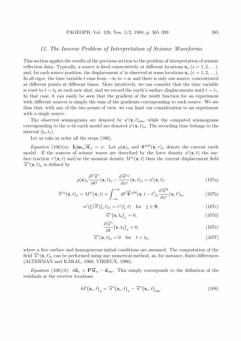
11. The Inverse Problem of Interpretation of Seismic Waveforms
This section applies the results of the previous section to the problem of interpretation of seismicreflection data. Typically, a source is fired consecutively at different locations xs (s = 1, 2, . . .),and, for each source position, the displacement ui is observed at some locations xr (r = 1, 2, . . .).In all rigor, the time variable t runs from −∞ to +∞ and there is only one source, concentratedat different points at different times. More intuitively, we can consider that the time variableis reset to t = t0 at each new shot, and we record the earth’s surface displacements until t = t1.In that case, it can easily be seen that the gradient of the misfit function for an experimentwith different sources is simply the sum of the gradients corresponding to each source. We seethus that, with any of the two points of view, we can limit our consideration to an experimentwith a single source.
The observed seismograms are denoted by ui(x, t)obs, while the computed seismogramscorresponding to the n-th earth model are denoted ui(x, t)n. The recording time belongs to theinterval [t0, t1).
Let us take in order all the steps (106).
Equation (106)(a): L[mn]−→u n = ψ. Let ρ(x)n and Ψijkl(x, τ)n denote the current earthmodel. If the sources of seismic waves are described by the force density φi(x, t) the sur-face traction τ i(x, t) and/or the moment density M ij(x, t) then the current displacement field−→u i(x, t)n is defined by
ρ(x)n∂2−→u i
∂t2(x, t)n −
∂−→σ ij
∂xj(x, t)n = φi(x, t), (107a)
−→σ ij(x, t)n = M ij(x, t) +
∫ +∞
−∞dt′−→Ψ ijkl(x, t− t′)n
∂−→u k
∂xl(x, t′)n, (107b)
nj(ξ)−→σ (ξ, t)n = τ i(ξ, t) for ξ ∈ S, (107c)
−→u i(x, t0
)n
= 0, (107d)
∂−→u i
∂t
(x, t0
)n
= 0, (107e)
−→u i(x, t)n = 0 for t < t0, (107f)
where a free surface and homogeneous initial conditions are assumed. The computation of thefield −→u i(x, t)n can be performed using any numerical method, as, for instance, finite-differences(ALTERMAN and KARAL, 1968; VIRIEUX, 1986).
Equation (106)(b): δdn = P−→u n − dobs. This simply corresponds to the definition of theresiduals at the receiver locations:
δdi(xr, t
)n
= −→u i(xr, t
)n−−→u i
(xr, t
)obs. (108)
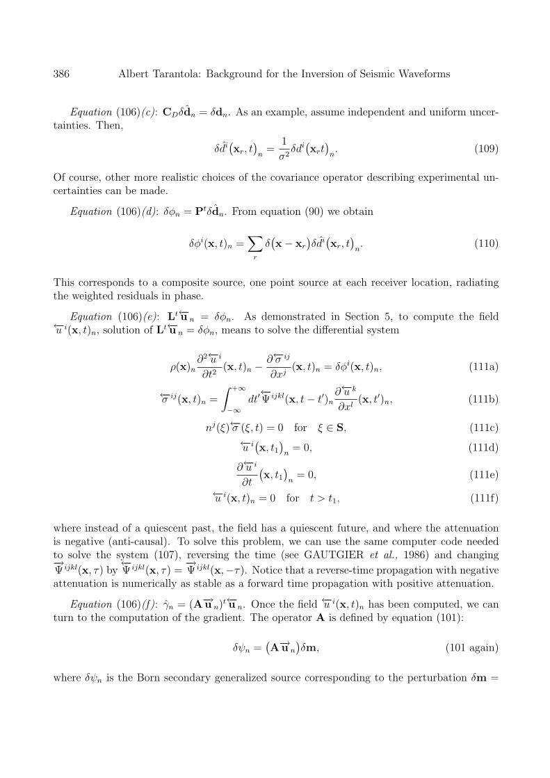
386 Albert Tarantola: Background for the Inversion of Seismic Waveforms
Equation (106)(c): CDδdn = δdn. As an example, assume independent and uniform uncer-tainties. Then,
δdi(xr, t
)n
=1
σ2δdi
(xrt
)n. (109)
Of course, other more realistic choices of the covariance operator describing experimental un-certainties can be made.
Equation (106)(d): δφn = Ptδdn. From equation (90) we obtain
δφi(x, t)n =∑
r
δ(x− xr
)δdi
(xr, t
)n. (110)
This corresponds to a composite source, one point source at each receiver location, radiatingthe weighted residuals in phase.
Equation (106)(e): Lt←−u n = δφn. As demonstrated in Section 5, to compute the field←−u i(x, t)n, solution of Lt←−u n = δφn, means to solve the differential system
ρ(x)n∂2←−u i
∂t2(x, t)n −
∂←−σ ij
∂xj(x, t)n = δφi(x, t)n, (111a)
←−σ ij(x, t)n =
∫ +∞
−∞dt′←−Ψ ijkl(x, t− t′)n
∂←−u k
∂xl(x, t′)n, (111b)
nj(ξ)←−σ (ξ, t) = 0 for ξ ∈ S, (111c)
←−u i(x, t1
)n
= 0, (111d)
∂←−u i
∂t
(x, t1
)n
= 0, (111e)
←−u i(x, t)n = 0 for t > t1, (111f)
where instead of a quiescent past, the field has a quiescent future, and where the attenuationis negative (anti-causal). To solve this problem, we can use the same computer code neededto solve the system (107), reversing the time (see GAUTGIER et al., 1986) and changing−→Ψ ijkl(x, τ) by
←−Ψ ijkl(x, τ) =
−→Ψ ijkl(x,−τ). Notice that a reverse-time propagation with negative
attenuation is numerically as stable as a forward time propagation with positive attenuation.
Equation (106)(f): γn = (A−→u n)t←−u n. Once the field ←−u i(x, t)n has been computed, we canturn to the computation of the gradient. The operator A is defined by equation (101):
δψn =(A−→u n
)δm, (101 again)
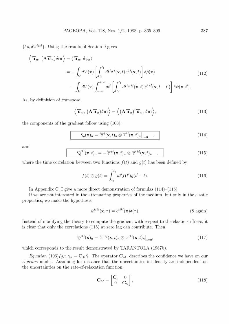
where δψn is the Born secondary generalized source corresponding to the perturbation δm =
PAGEOPH, Vol. 128, Nos. 1/2, 1988, p. 365–399 387
{δρ, δΨijkl}. Using the results of Section 9 gives⟨←−u n,(A−→u n
)δm
⟩=
⟨←−u n, δψn
⟩= +
∫V
dV (x)
[∫ t1
t0
dt←−v i(x, t)−→v i(x, t)
]δρ(x)
−∫
V
dV (x)
∫ +∞
−∞dt′
[∫ t1
t0
dt←−ε ij(x, t)−→ε kl(x, t− t′)]δψ(x, t′).
(112)
As, by definition of transpose,⟨←−u n,(A−→u n
)δm
⟩=
⟨(A−→u n
)t←−u n, δm⟩, (113)
the components of the gradient follow using (103):
γρ(x)n =←−v i(x, t)n ⊗−→v i(x, t)n
∣∣t=0
, (114)
and
γijklΨ (x, t)n = −←−ε ij(x, t)n ⊗−→ε kl(x, t)n , (115)
where the time correlation between two functions f(t) and g(t) has been defined by
f(t)⊗ g(t) =
∫ t1
t0
dt′f(t′)g(t′ − t). (116)
In Appendix C, I give a more direct demonstration of formulas (114)–(115).If we are not interested in the attenuating properties of the medium, but only in the elastic
properties, we make the hypothesis
Ψijkl(x, τ) = cijkl(x)δ(τ). (8 again)
Instead of modifying the theory to compute the gradient with respect to the elastic stiffness, itis clear that only the correlations (115) at zero lag can contribute. Then,
γijklc (x)n =←−ε ij(x, t)n ⊗−→ε kl(x, t)n
∣∣t=0, (117)
which corresponds to the result demonstrated by TARANTOLA (1987b).
Equation (106)(g): γn = CM γ. The operator CM , describes the confidence we have on oura priori model. Assuming for instance that the uncertainties on density are independent onthe uncertainties on the rate-of-relaxation function,
CM =
[Cρ 00 CΨ
], (118)
388 Albert Tarantola: Background for the Inversion of Seismic Waveforms
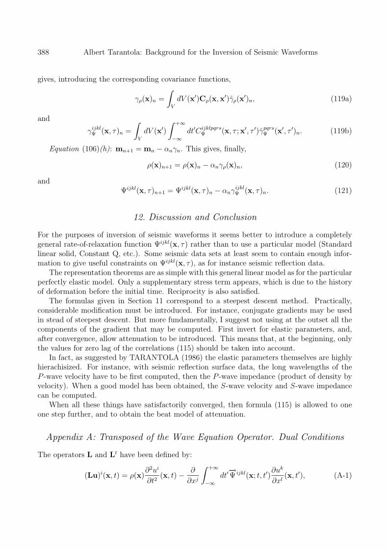
gives, introducing the corresponding covariance functions,
γρ(x)n =
∫V
dV (x′)Cρ(x,x′)γρ(x
′)n, (119a)
and
γijklΨ (x, τ)n =
∫V
dV (x′)
∫ +∞
−∞dt′Cijklpqrs
Ψ (x, τ ;x′, τ ′)γpqrsΨ (x′, τ ′)n. (119b)
Equation (106)(h): mn+1 = mn − αnγn. This gives, finally,
ρ(x)n+1 = ρ(x)n − αnγρ(x)n, (120)
andΨijkl(x, τ)n+1 = Ψijkl(x, τ)n − αnγ
ijklΨ (x, τ)n. (121)
12. Discussion and Conclusion
For the purposes of inversion of seismic waveforms it seems better to introduce a completelygeneral rate-of-relaxation function Ψijkl(x, τ) rather than to use a particular model (Standardlinear solid, Constant Q, etc.). Some seismic data sets at least seem to contain enough infor-mation to give useful constraints on Ψijkl(x, τ), as for instance seismic reflection data.
The representation theorems are as simple with this general linear model as for the particularperfectly elastic model. Only a supplementary stress term appears, which is due to the historyof deformation before the initial time. Reciprocity is also satisfied.
The formulas given in Section 11 correspond to a steepest descent method. Practically,considerable modification must be introduced. For instance, conjugate gradients may be usedin stead of steepest descent. But more fundamentally, I suggest not using at the outset all thecomponents of the gradient that may be computed. First invert for elastic parameters, and,after convergence, allow attenuation to be introduced. This means that, at the beginning, onlythe values for zero lag of the correlations (115) should be taken into account.
In fact, as suggested by TARANTOLA (1986) the elastic parameters themselves are highlyhierachisized. For instance, with seismic reflection surface data, the long wavelengths of theP -wave velocity have to be first computed, then the P -wave impedance (product of density byvelocity). When a good model has been obtained, the S-wave velocity and S-wave impedancecan be computed.
When all these things have satisfactorily converged, then formula (115) is allowed to oneone step further, and to obtain the beat model of attenuation.
Appendix A: Transposed of the Wave Equation Operator. Dual Conditions
The operators L and Lt have been defined by:
(Lu)i(x, t) = ρ(x)∂2ui
∂t2(x, t)− ∂
∂xj
∫ +∞
−∞dt′−→Ψ ijkl(x; t, t′)
∂uk
∂xl(x, t′), (A-1)
PAGEOPH, Vol. 128, Nos. 1/2, 1988, p. 365–399 389
and
(Ltu)i(x, t) = ρ(x)∂2ui
∂t2(x, t)− ∂
∂xj
∫ +∞
−∞dt′←−Ψ ijkl(x; t, t′)
∂uk
∂xl(x, t′), (A-2)
where−→Ψ jikl(x; t, t′) is a causal function,
−→Ψ ijkl(x; t, t′) = 0 for t < t′, (A-3)
and ←−Ψ ijkl(x; t, t′) =
−→Ψ ijkl(x; t′, t). (A-4)
We have
〈←−u ,L−→u 〉Φ −⟨Lt←−u ,−→u
⟩U
=
∫V
dV (x)
∫ t1
t0
dt←−u i(x, t)(L−→u )i(x, t)
−∫
V
dV (x)
∫ t1
t0
dt(Lt←−u
)i(x, t)−→u i(x, t),
and, inserting (A-1) and (A-2),
〈←−u ,L−→u 〉Φ −⟨Lt←−u ,−→u
⟩U
= A+B, (A-5)
where
A =
∫V
dV (x)ρ(x)
∫ t1
t0
dt
[←−u i(x, t)
∂2−→u i
∂t2(x, t)− ∂2←−u i
∂t2(x, t)−→u i(x, t)
], (A-6)
and
B =−∫
V
dV (x)
∫ t1
t0
dt←−u i(x, t)
[∂
∂xj
∫ +∞
−∞dt′−→Ψ ijkl(x; t, t′)
∂−→u k
∂xl(x, t′)
]+
∫V
dV (x)
∫ t1
t0
dt
[∂
∂xj
∫ +∞
−∞dt′←−Ψ ijkl(x; t, t′)
∂←−u k
∂xl(x, t′)
]−→u i(x, t).
(A-7)
As∂
∂t
[←−u i∂−→u i
∂t− ∂←−u i
∂t−→u i
]=←−u i∂
2−→u i
∂t2− ∂2←−u i
∂t2−→u i,
we have
A =
∫V
dV (x)ρ(x)
[←−u i(x, t)
∂2−→u i
∂t2(x, t)− ∂2←−u i
∂t2(x, t)−→u i(x, t)
] ∣∣∣∣t=t1
t=t0
. (A-8)
Equation (A-7) can be rewrittenB = C +D, (A-9)
where
C =−∫
V
dV (x)
∫ t1
t0
dt∂
∂xj
[←−u i(x, t)
[ ∫ +∞
−∞dt′−→Ψ ijkl(x; t, t′)
∂−→u k
∂xl(x, t′)
]]
+
∫V
dV (x)
∫ t1
t0
dt∂
∂xj
[[ ∫ +∞
−∞dt′←−Ψ ijkl(x; t, t′)
∂←−u k
∂xl(x, t′)
]−→u i(x, t)
],
(A-10)
390 Albert Tarantola: Background for the Inversion of Seismic Waveforms
and
D = +
∫V
dV (x)
∫ t1
t0
dt∂←−u i
∂xj(x, t)
[∫ +∞
−∞dt′−→Ψ ijkl(x; t, t′)
∂−→u k
∂xl(x, t′)
]=
∫V
dV (x)
∫ t1
t0
dt
[∫ +∞
−∞dt′←−Ψ ijkl(x; t, t′)
∂←−u k
∂xl(x, t′)
]∂−→u i
∂xj(x, t).
(A-11)
Using the divergence theorem gives
C =−∫
s
dS(ξ)
∫ t1
t0
dt←−u i(ξ, t)
[nj(ξ)
∫ +∞
−∞dt′−→Ψ ijkl(ξ; t, t′)
∂−→u k
∂xl(ξ, t′)
]+
∫s
dS(ξ)
∫ t1
t0
dt
[nj(ξ)
∫ +∞
−∞dt′←−Ψ ijkl(ξ; t, t′)
∂←−u k
∂xl(ξ, t′)
]−→u i(ξ, t).
(A-12)
The term D can be rewritten
D = +
∫V
dV (x)
∫ t1
t0
dt∂←−u i
∂xj(x, t)
[[ ∫ t0
−∞dt′ +
∫ t1
t0
dt′ +
∫ +∞
t1
dt′
]−→Ψ ijkl(x; t, t′)
∂−→u k
∂xl(x, t′)
]
−∫
V
dV (x)
∫ t1
t0
dt
[[ ∫ t0
−∞dt′ +
∫ t1
t0
dt′
+
∫ +∞
t1
dt′
]←−Ψ ijkl(x; t, t′)
∂←−u k
∂xl(x, t′)
]∂−→u i
∂xj(x, t),
or, using the causality and anti-causality properties−→Ψ ijkl(x; t, t′) and
←−Ψ ijkl(x; t, t′) respectively,
D =
∫V
dV (x)
∫ t1
t0
dt∂←−u i
∂xj(x, t)
[[ ∫ t0
−∞dt′ +
∫ t1
t0
dt′
]−→Ψ ijkl(x; t, t′)
∂−→u k
∂xl(x, t′)
]
−∫
V
dV (x)
∫ t1
t0
dt
[[ ∫ t1
t0
dt′ +
∫ +∞
t1
dt′
]←−Ψ ijkl(x; t, t′)
∂←−u k
∂xl(x, t′)
]∂−→u i
∂xj(x, t),
i.e.,D = E + F, (A-13)
where
E = +
∫V
dV (x)
∫ t1
t0
dt
∫ t1
t0
dt′∂←−u i
∂xj(x, t)
−→Ψ ijkl(x; t, t′)
∂−→u k
∂xl(x, t′)
−∫
V
dV (x)
∫ t1
t0
dt
∫ t1
t0
dt′←−Ψ ijkl(x; t, t′)
∂←−u k
∂xl(x, t′)
∂−→u i
∂xj(x, t),
(A-14)
and
F = +
∫V
dV (x)
∫ t1
t0
dt∂←−u i
∂xj(x, t)
[∫ t0
−∞dt′−→Ψ ijkl(x; t, t′)
∂−→u k
∂xl(x, t′)
]−
∫V
dV (x)
∫ t1
t0
dt
[∫ +∞
t1
dt′←−Ψ ijkl(x; t, t′)
∂←−u k
∂xl(x, t′)
]∂−→u i
∂xj(x, t).
(A-15)
PAGEOPH, Vol. 128, Nos. 1/2, 1988, p. 365–399 391
Using (A-4) and the symmetries between indexes ij and kj gives
E = 0. (A-16)
This ends the proof for equation (39) of the text.
Appendix B: Representation Theorem
Let←−G ij(x, t;x′, t′) be defined by
ρ(x)∂2←−G ip
∂t2(x, t;x′, t′)− ∂
∂xj
∫ +∞
−∞dt′′−→Ψ ijkl(x; t, t′′)
∂←−G kp
∂xl(x, t′′;x′, t′)
= δipδ(x− x′)δ(t− t′),
(B-1a)
←−G ip(x, t;x′, t′) = 0 for t ≥ t′ (B-1b)
∂←−G ip
∂t(x, t;x′, t′) = 0 for t ≥ t′, (B-1c)
where←−Ψ ijkl(x; t, t′) is anti-causal:
←−Ψ ijkl(x; t, t′) = 0 for t > t′. (B-2)
For an arbitrary function ui(x, t) we have, for any t′, t0 < t′ < t1,
up(x′, t′) =
∫V
dV (x)
∫ t1
t0
dtδipδ(x− x′)δ(t− t′)ui(x, t). (B-3)
Inserting (B-1a), into (B-3) gives
up(x′, t′) = A+B, (B-4)
where
A =
∫V
dV (x)ρ(x)
∫ t1
t0
dt∂2←−G ip
∂t2(x, t;x′, t′)ui(x, t), (B-5)
and
B = −∫
V
dV (x)
∫ t1
t0
dt
[∂
∂xj
∫ +∞
−∞dt′′←−Ψ ijkl(x; t, t′′)
∂←−G kp
∂xl(x, t′′;x′, t′)
]ui(x, t). (B-6)
As∂2←−G ip
∂t2ui =
∂
∂t
[∂←−G ip
∂t2ui −
←−G ip∂u
i
∂t
]+←−G ip∂
2ui
∂t2,
392 Albert Tarantola: Background for the Inversion of Seismic Waveforms
and, as←−G ip(x, t;x′, t′) is anti-causal, we have
A =
∫V
dV (x)
∫ t1
t0
dt←−G ip(x, t;x′, t′)ρ(x)
∂2ui
∂t2(x, t)
−∫
V
dV (x)ρ(x)
[∂←−G ip
∂t
(x, t0;x
′, t′)ui
(x, t0
)−←−G ip
(x, t0;x
′, t′)∂ui
∂t
(x, t0
)].
(B-7)
Equation (B-6) can be rewrittenB = C +D, (B-8)
where
C = −∫
V
dV (x)
∫ t1
t0
dt∂
∂xj
[∫ +∞
−∞dt′′←−Ψ ijkl(x; t, t′′)
∂←−G kp
∂xl(x, t′′;x′, t′)
]ui(x, t), (B-9)
and
D = +
∫V
dV (x)
∫ t1
t0
dt
[∫ +∞
−∞dt′′←−Ψ ijkl(x; t, t′′)
∂←−G kp
∂xl(x, t′′;x′, t′)
]∂ui
∂xj(x, t). (B-10)
Using the divergence theorem gives
C = −∫
s
dS(ξ)
∫ t1
t0
dt
[nj(ξ)
∫ +∞
−∞dt′′←−Ψ ijkl(x; t, t′′)
∂←−G kp
∂xl(x, t′′;x′, t′)
]ui(x, t). (B-11)
Using ←−Ψ ijkl(x; t, t′′) =
−→Ψ ijkl(x; t′′, t) (B-12)
changing t↔ t′′, ij ↔ kl and reordering gives
D =
∫V
dV (x)
∫ +∞
−∞dt∂←−G ip
∂xj(x, t;x′, t′)
∫ t1
t0
dt′′−→Ψ ijkl(x; t, t′′)
∂uk
∂xl(x, t′′). (B-13)
The anti-causality property of←−G ip(x, t;x′, t′) and the causality property of
−→Ψ ijkl(x; t, t′) allow
to change the bounds of integration:
D =
∫V
DV (x)
∫ t1
t0
dt∂←−G ip
∂xj(x, t;x′, t′)
∫ +∞
t0
dt′′−→Ψ ijkl(x; t, t′′)
∂uk
∂xl(x, t′′), (B-14)
i.e.,
D =
∫V
dV (x)
∫ t1
t0
dt∂←−G ip
∂xj(x, t;x′, t′)
[ ∫ +∞
−∞dt′′ −
∫ t0
−∞dt′′
]−→Ψ ijkl(x; t, t′′)
∂uk
∂xl(x, t′′). (B-15)
This givesD = E + F, (B-16)
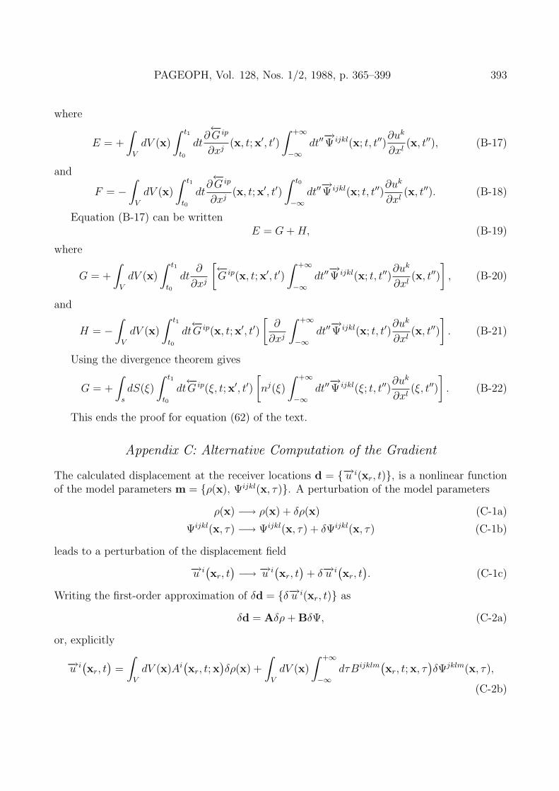
PAGEOPH, Vol. 128, Nos. 1/2, 1988, p. 365–399 393
where
E = +
∫V
dV (x)
∫ t1
t0
dt∂←−G ip
∂xj(x, t;x′, t′)
∫ +∞
−∞dt′′−→Ψ ijkl(x; t, t′′)
∂uk
∂xl(x, t′′), (B-17)
and
F = −∫
V
dV (x)
∫ t1
t0
dt∂←−G ip
∂xj(x, t;x′, t′)
∫ t0
−∞dt′′−→Ψ ijkl(x; t, t′′)
∂uk
∂xl(x, t′′). (B-18)
Equation (B-17) can be writtenE = G+H, (B-19)
where
G = +
∫V
dV (x)
∫ t1
t0
dt∂
∂xj
[←−G ip(x, t;x′, t′)
∫ +∞
−∞dt′′−→Ψ ijkl(x; t, t′′)
∂uk
∂xl(x, t′′)
], (B-20)
and
H = −∫
V
dV (x)
∫ t1
t0
dt←−G ip(x, t;x′, t′)
[∂
∂xj
∫ +∞
−∞dt′′−→Ψ ijkl(x; t, t′)
∂uk
∂xl(x, t′′)
]. (B-21)
Using the divergence theorem gives
G = +
∫s
dS(ξ)
∫ t1
t0
dt←−G ip(ξ, t;x′, t′)
[nj(ξ)
∫ +∞
−∞dt′′−→Ψ ijkl(ξ; t, t′′)
∂uk
∂xl(ξ, t′′)
]. (B-22)
This ends the proof for equation (62) of the text.
Appendix C: Alternative Computation of the Gradient
The calculated displacement at the receiver locations d = {−→u i(xr, t)}, is a nonlinear functionof the model parameters m = {ρ(x), Ψijkl(x, τ)}. A perturbation of the model parameters
ρ(x) −→ ρ(x) + δρ(x) (C-1a)
Ψijkl(x, τ) −→ Ψijkl(x, τ) + δΨijkl(x, τ) (C-1b)
leads to a perturbation of the displacement field
−→u i(xr, t
)−→ −→u i
(xr, t
)+ δ−→u i
(xr, t
). (C-1c)
Writing the first-order approximation of δd = {δ−→u i(xr, t)} as
δd = Aδρ+ BδΨ, (C-2a)
or, explicitly
−→u i(xr, t
)=
∫V
dV (x)Ai(xr, t;x
)δρ(x) +
∫V
dV (x)
∫ +∞
−∞dτBijklm
(xr, t;x, τ
)δΨjklm(x, τ),
(C-2b)
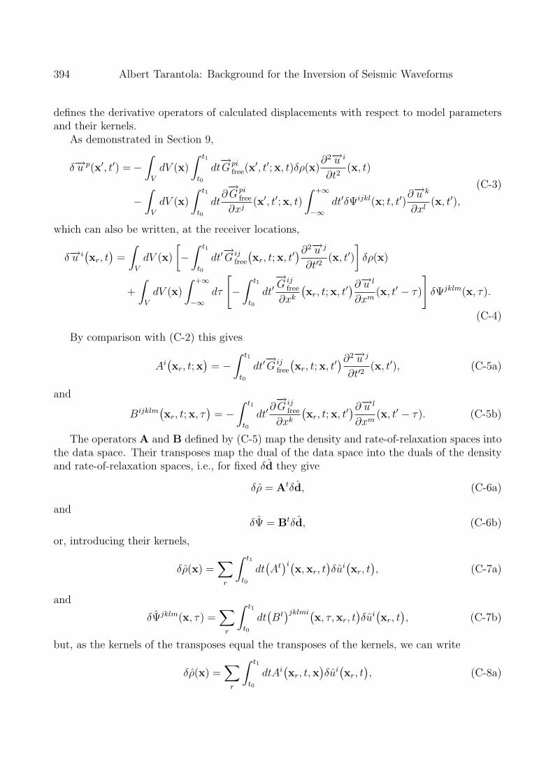
394 Albert Tarantola: Background for the Inversion of Seismic Waveforms
defines the derivative operators of calculated displacements with respect to model parametersand their kernels.
As demonstrated in Section 9,
δ−→u p(x′, t′) =−∫
V
dV (x)
∫ t1
t0
dt−→G pi
free(x′, t′;x, t)δρ(x)
∂2−→u i
∂t2(x, t)
−∫
V
dV (x)
∫ t1
t0
dt∂−→G pi
free
∂xj(x′, t′;x, t)
∫ +∞
−∞dt′δΨijkl(x; t, t′)
∂−→u k
∂xl(x, t′),
(C-3)
which can also be written, at the receiver locations,
δ−→u i(xr, t
)=
∫V
dV (x)
[−
∫ t1
t0
dt′−→G ij
free
(xr, t;x, t
′)∂2−→u j
∂t′2(x, t′)
]δρ(x)
+
∫V
dV (x)
∫ +∞
−∞dτ
[−
∫ t1
t0
dt′−→G ij
free
∂xk
(xr, t;x, t
′)∂−→u l
∂xm(x, t′ − τ)
]δΨjklm(x, τ).
(C-4)
By comparison with (C-2) this gives
Ai(xr, t;x
)= −
∫ t1
t0
dt′−→G ij
free
(xr, t;x, t
′)∂2−→u j
∂t′2(x, t′), (C-5a)
and
Bijklm(xr, t;x, τ
)= −
∫ t1
t0
dt′∂−→G ij
free
∂xk
(xr, t;x, t
′)∂−→u l
∂xm(x, t′ − τ). (C-5b)
The operators A and B defined by (C-5) map the density and rate-of-relaxation spaces intothe data space. Their transposes map the dual of the data space into the duals of the densityand rate-of-relaxation spaces, i.e., for fixed δd they give
δρ = Atδd, (C-6a)
andδΨ = Btδd, (C-6b)
or, introducing their kernels,
δρ(x) =∑
r
∫ t1
t0
dt(At
)i(x,xr, t
)δui
(xr, t
), (C-7a)
and
δΨjklm(x, τ) =∑
r
∫ t1
t0
dt(Bt
)jklmi(x, τ,xr, t
)δui
(xr, t
), (C-7b)
but, as the kernels of the transposes equal the transposes of the kernels, we can write
δρ(x) =∑
r
∫ t1
t0
dtAi(xr, t,x
)δui
(xr, t
), (C-8a)
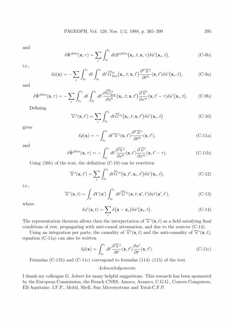
PAGEOPH, Vol. 128, Nos. 1/2, 1988, p. 365–399 395
and
δΨjklm(x, τ) =∑
r
∫ t1
t0
dtBijklm(xr, t,x, τ
)δui
(xr, t
), (C-8b)
i.e.,
δρ(x) = −∑
r
∫ t1
t0
dt
∫ t1
t0
dt′−→G ij
free
(xr, t;x, t
′)∂2−→u j
∂t′2(x, t′)δui
(xr, t
), (C-9a)
and
δΨjklm(x, τ) = −∑
r
∫ t1
t0
dt
∫ t1
t0
dt′∂−→G ij
free
∂xk
(xr, t;x, t
′)∂−→u l
∂xm(x, t′ − τ)δui
(xr, t
). (C-9b)
Defining
←−u j(x, t′) =∑
r
∫ t1
t0
dt−→G ij
(xr, t;x, t
′)δui(xr, t
)(C-10)
gives
δρ(x) = −∫ t1
t0
dt′←−u j(x, t′)∂2−→u j
∂t′2(x, t′), (C-11a)
and
δΨjklm(x, τ) = −∫ t1
t0
dt′∂←−u j
∂xk(x, t′)
∂−→u l
∂xm(x, t′ − τ). (C-11b)
Using (56b) of the text, the definition (C-10) can be rewritten
←−u j(x, t′) =∑
r
∫ t1
t0
dt←−G ji
(x, t′;xr, t
′)δui(xr, t
), (C-12)
i.e.,
←−u i(x, t) =
∫V
dV (x′)
∫ t1
t0
dt′←−G ij(x, t;x′, t′)δφj(x′, t′), (C-13)
whereδφi(x, t) =
∑r
δ(x− xr
)δui
(xr, t
). (C-14)
The representation theorem allows then the interpretation of ←−u i(x, t) as a field satisfying finalconditions of rest, propagating with anti-causal attenuation, and due to the sources (C-14).
Using an integration per parts, the causality of −→u i(x, t) and the anti-causality of ←−u i(x, t),equation (C-11a) can also be written
δρ(x) =
∫ t1
t0
dt′∂←−u j
∂t′(x, t′)
∂uj
∂t′(x, t′). (C-11c)
Formulas (C-11b) and (C-11c) correspond to formulas (114)–(115) of the text.
Acknowledgements
I thank my colleague G. Jobert for many helpful suggestions. This research has been sponsoredby the European Commission, the French CNRS, Amoco, Aramco, C.G.G., Convex Computers,Elf-Aquitaine, I.F.P., Mobil, Shell, Sun Microsystems and Total-C.F.P.
396 Albert Tarantola: Background for the Inversion of Seismic Waveforms
References and References for General Reading
AKI, K. and RICHARDS, P. G. (1980), Quantitative Seismology (2 volumes) (Freeman andCo.).
ALTERMAN, Z. S. and KARAL, F. C., Jr. (1968), Propagation of elastic waves in layeredmedia by finite difference methods, Bull. Seismol. Soc. of America 58, 367–398.
BACKUS, G. (1970), Inference from inadequate and inaccurate data: I, Proceedings of theNational Academy of Sciences 65, 1, 1–105.
BACKUS, G. (1970), Inference from inadequate and inaccurate data: II, Proceedings of theNational Academy of Sciences 65, 2, 281–287.
BACKUS, G. (1970), Inference from inadequate and inaccurate data: III, Proceedings of theNational Academy of Sciences 67, 1, 282–289.
BACKUS, G. and GILBERT, F. (1967), Numerical applications of a formalism for geophysicalinverse problems, Geophys. J. R. Astron. Soc. 13, 247–276.
BACKUS, G. and GILBERT, F. (1968), The resolving power of gross Earth data, Geophys. J.R. Astron. Soc. 16, 169–205.
BACKUS, G. and GILBERT, F. (1970), Uniqueness in the inversion of inaccurate gross Earthdata, Philos. Trans. R. Soc. London 266, 123–192.
BACKUS, G. (1971), Inference from inadequate and inaccurate data, Mathematical problemsin the Geophysical Sciences: Lecture in Applied Mathematics, 14, American MathematicalSociety, Providence, Rhode Island.
BALAKRISHNAN, A. V., Applied Functional Analysis (Springer-Verlag, 1976).BAMBERGER, A., CHAVENT, G., HEMON, Ch., and LAILLY, P. (1982), Inversion of normal
incidence seismograms, Geophysics 47, 757–770.BEN-MENAHEM, A. and SINGH, S. J., Seismic Waves and Sources (Springer-Verlag, 1981).BENDER, C. M. and ORSZAG, S. A., Advanced Mathematical Methods for Scientists and
Engineers (McGraw-Hill, 1978).BERKHOUT, A. J., Seismic Migration, Imaging of Acoustic Energy by Wave Field Extrapola-
tion (Elsevier, 1980).BEYDOWN, W. (1985), Asymptotic wave methods in heterogeneous media, Ph.D Thesis, Mas-
sachusetts Institute of Technology.BLAND, D. R., The Theory of Linear Viscoelasticity (Pergamon Press, 1960).BLEISTEIN, N., Mathematical Methods for Wave Phenomena (Academic Press, 1984).BOURBIE, T., COUSSY, O., and ZINSZNER, B. (1986), Acoustique des milieux poreux, Tech-
nip, 1986.BOSCHI, E. (1973), Body force equivalents for dislocations in visco-elastic media, J. Geophys.
Res. 78, 32, 7727–8590.CLAERBOUT, J. F. (1971), Toward a unified theory of reflector mapping, Geophysics 36,
467–481.CLAERBOUT, J. F., Fundamentals of Geophysical Data Processing (McGraw-Hill, 1976).CLAERBOUT, J. F., Imaging the Earth’s Interior (Blackwell, 1985).CLAERBOUT, J. F. and MUIR, F. (1973), Robust modelling with erratic data, Geophysics 38,
5, 826–844.
PAGEOPH, Vol. 128, Nos. 1/2, 1988, p. 365–399 397
COURANT, R. and HILBERT, D., Methods of Mathematical Physics (Interscience Publishers,1953).
DAUTRAY, R. and LIONS, J. L., Analyse mathematique et calcul numerique pour les scienceset les techniques (3 volumes) (Masson, Paris, 1984 and 1985).
DAVIDON, W. C. (1959), Variable metric method for minimization, AEC Res. and Dev.,Report ANL-5990 (revised).
DEVANEY, A. J. (1984), Geophysical diffraction tomography, IEEE Trans. Geos. RemoteSensing GE-22, No. 1.
FLETCHER, R., Practical Methods of Optimization, Volume 1: Unconstrained Optimization(Wiley, 1980).
FLETCHER, R., Practical Methocis of Optimization, Volume 2: Constrained Optimization(Wiley, 1981).
FRANKLIN, J. N. (1970), Well posed stochastic extensions of ill posed linear problems, J. Math.Anal. Applic. 31, 682–716.
GAUTHIER, O., VIRIEUX, J., and TARANTOLA, A. (1986), Two-dimensional inversion ofseismic waveforms: Numerical results, Geophysics 51, 1387–1403.
HAMILTON, E. L. (1972), Compressional-wave attenuation in marine sediments, Geophysics37, 620–646.
HERMAN, G. T., Image reconstruction from projections, the fundamentals of computerizedtomography (Academic Press, 1980).
HSI-PING Liu, ANDERSON, D. L., and KANAMORI, H. (1976), Velocity dispersion due toanelasticity; implications for seismology and mantle composition, Geophys. J. R. Astr. Soc.47, 41–58.
IKELLE, L. T., DIET, J. P., and TARANTOLA, A. (1986), Linearized inversion of multi offsetseismic reflection data in the w-k domain, Geophysics 51, 1266–1276.
JACOBSON, R. S. (1987), An investigation into the fundamental relationships between atten-uation, phase dispersion, and frequency using seismic refraction profiles over sedimentarystructures, Geophysics 52, 72–87.
JOHNSON, L. R. (1974), Green’s function for Lamb’s problem, Geophys. J. R. Astr. Soc. 37,99–131.
KENNETT, B,. L. N. (1974), On variational principles and matrix methods in elastodynamics,Geophys. J. R. Astr. Soc. 37, 391–405.
KENNETT, B. L. N. (1978) Some aspects of non-linearity in inversion, Geophys. J. R. Astr.Soc. 55, 373–391.
KJARTANSSON, E. (1979), Constant Q-wave propagation and attenuation, J. Geoph. Res.84, B9, 4737–4748.
KOLB, P., COLLINO, F., and LAILLY, P. (1986), Pre-stack inversion of a ID medium, Pro-ceedings of the IEEE 74, 3, 498–508.
LICKNEROWICZ, A., Elements de Culcul Tensoriel (Armand Collin, Paris, 1960).
LIONS, J. L., Controle optimal de systemes gouvernes par des equations aux derivees partielles(Dunod, Paris, 1968). English translation: Optimal control of systems governed by partialdtflerential equations (Springer, 1971).
398 Albert Tarantola: Background for the Inversion of Seismic Waveforms
Liu, H. P., ANDERSON, D. L., and KANAMORI, H. (1976), Velocity dispersion due to anelas-ticity; implications for seismology and mantle composition, Geophys. J. R. Astr. Soc. 47,41–58.
MILNE, R. D., Applied Functional Analysis (Pitman Advanced Publishing Program, Boston,1980).
MISNER, Ch. W., THORNE, K. S., and WHEELER, J. A., Gravitation (Freeman, 1973).
MORA, P. (1988), Elastic wavefield inversion of reflection and transmission data, Geophysics53, 750–759.
MORITZ, H., Advanced Physical Geodesy (Herbert Wichmann Verlag, Karlsruhe, AbacusPress, Tunbridge Wells, Kent, 1980).
MORSE, P. M. and FESHBACH, H., Methods of Theoretical Physics (McGraw-Hill, 1953).
NERCESSIAN, A., HIRN, A., and TARANTOLA, A. (1984) Three-dimensional seismic trans-mission prospecting of the Mont-Dore volcano, France, Geophys. J. R. Astr. Soc. 76,307–315.
NOLET, G. (1985), Solving or resolving inadequate and noisy tomographic systems, J. Comp.Phys. 61, 463–482.
O’CONNELL, R. J. and BUDIANSKY, B. (1978), Measures of dissipation in viscoelastic media,Geophysical Research Letters 5, 1, 5–8.
PARK, J. and GILBERT, F. (1986), Coupled free oscillations of an aspherical, dissipative,rotating Earth: Galerkin theory, J. Geoph. Res. 91, B7, 7241–7260.
PARKER, R. L. (1975), The theory of ideal bodies for gravity interpretation, Geophys, J. R.Astron. Soc. 42, 315–334.
PARKER, R. L. (1977), Understanding inverse theory, Ann. Rev. Earth Plan. Sci. 5, 35–64.
PICA, A., DIET, J. P., and TARANTOLA, A. (1988), Practice of nonlinear inversion of realseismic reflection data in a laterally invariant medium, submitted to Geophysics.
POLACK, E. and RIBIERE, G. (1969), Note sur la convergence de methodes de directionsconjuguees, Revue Fr. Inf. Rech. Oper. 16-R1, 35–43.
POWELL, M. J. D., Approximation Theory and Methods (Cambridge University Press, 1981).
RAZAVY, M. and LEONACH, B. (1986), Reciprocity principle and the approximate solutionof the wave equation, Bull. Seism. Soc. of America 76, 1776–1789.
RICKER, N. H., Transient Waves in Visco-elastic Media (Elsevier, 1977).
SCALES, L. E., Introduction to Non-linear Optimization (Macmillan, 1985).
SCHOENBERGER, M. and LEVIN, F. K. (1974), Apparent attenuation due to intrubed mul-tiples, Geophysics 39, 278–291.
SCHWARTZ, L., Methodes mathematiques pour les sciences physiques (Hermann, Paris, 1965).
SCHWARTZ, L., Theorie des distributions (Hermann, Paris, 1966).
SCHWARTZ, L., Analyse (topologie generale et analyse fonctionelle) (Hermann, Paris, 1970).
TANIMOTO, A. (1985), The Backus-Gilbert approach to the three-dimensional structure inthe upper mantle.—I. Lateral variation of surface wave phase velocity with its error andresolution, Geophys. J. R. Astr. Soc. 82, 105–123.
TARANTOLA, A. (1984a), Linearized inversion of seismic reflection data, Geophysical Prospect-ing 32, 998–1015.
PAGEOPH, Vol. 128, Nos. 1/2, 1988, p. 365–399 399
TARANTOLA, A. (1984b), Inversion of seismic reflection data in the acoustic approximation,Geophysics 49, 1259–1266.
TARANTOLA, A., The seismic reflection inverse problem, in Inverse Problems of Acoustic andElastic Waves (edited by: F. Santosa, Y.-H. Pao, W. Symes, and Ch. Holland) (SIAM,Philadelphia, 1984).
TARANTOLA, A. (1986), A strategy for nonlinear elastic inversion of seismic reflection data,Geophysics 51, 1893–1903.
TARANTOLA, A., Inverse Problem Theory; Methods for Data Fitting and Model ParameterEstimation (Elsevier, 1987a).
TARANTOLA, A., Inversion of travel time and seismic waveforms, in Seismic Tomography(edited by G. Nolet) (Reidel, 1987b).
TARANTOLA, A., JOBERT, G., TREZEGUET, D., and DENELLE, E. (1988), Inversion ofseismic waveforms can either be performed by time or by depth extrapolation, GeophysicalProspecting 36, 383–416.
TARANTOLA, A. and NERCESSIAN, A. (1984), Three-dimensional inversion without blocks,Geophys. J. R. Astr. Soc. 76, 299–306.
TARANTOLA, A., and VALETTE, B. (1982a), Inverse Problems = Quest for Information, J.Geophys. 50, 159–170.
TARANTOLA, A. and VALETTE, B. (1982b), Generalized nonlinear inverse problems solvedusing the least squares criterion, Rev. Geophys. Space Phys. 20, 2, 219–232.
TAYLOR, A. E. and LAY, D. C., Introduction to Functional Analysis (Wiley, 1980).VIRIEUX, J. (1986), P-SV wave propagation in heterogeneous media; velocity-stress finite-
difference method, Geophysics 51, 889–901.WALSH, G. R., Methods of Optimization (Wiley, 1975).WATSON, G. A., Approximation Theory and Numerical Methods (Wiley, 1980).WOODHOUSE, J. H. (1974), Surface waves in a laterally varying layered structure, Geophys.
J. R. Astr. Soc. 37, 461–490.WOODHOUSE, J. H. and DZIEWONSKI, A. M. (1984), Mapping the upper mantle: Three-
dimensional modeling of Earth structure by inversion of seismic waveforms, Journal ofGeophysical Research 89, B7, 5953–5986.
WU, R.-S., and BEN-MENAHEM, A. (1985), The elastodynamic near field, Geophys. J. R.Astr. Soc. 81, 609–621.
(Received June 10, 1987, revised January 10, 1988, accepted January 11, 1988)