The Stability and Slow Dynamics of Localized Spot Patterns for the 3-D

Schnakenberg Reaction-Diffusion Model

J. C. Tzou∗ , S. Xie† , T. Kolokolnikov ‡ , M. J. Ward §

September 23, 2016

Abstract

On a bounded three-dimensional domain Ω, a hybrid asymptotic-numerical method is employed to analyze theexistence, linear stability, and slow dynamics of localized quasi-equilibrium multi-spot patterns of the Schnakenbergactivator-inhibitor model with bulk feed rate A in the singularly perturbed limit of small diffusivity ε2 of the activatorcomponent. By approximating each spot as a Coulomb singularity, a nonlinear system of equations is formulatedfor the strength of each spot. To leading order in ε, two types of solutions are identified: symmetric patterns forwhich all strengths are identical, and asymmetric patterns for which each strength takes on one of two distinct values.The O(ε) correction to the strengths is found to depend on the spatial configuration of the spots through a certainNeumann Green’s matrix G. When e = (1, . . . , 1)T is not an eigenvector of G, a detailed numerical and (in the case oftwo spots) asymptotic characterization is performed for the resulting imperfection-sensitive bifurcation structure. Forsymmetric multi-spot patterns, a leading-order global threshold in terms of |Ω| and parameters of the Schnakenbergmodel is obtained below which a competition instability is triggered leading to the annihilation of one or more spots.A corresponding refined threshold is established in terms of eigenvalues of G in the special case when Ge = ke.Additionally, a local self-replication threshold for the strength of each spot is derived numerically above which a spotsplits into two. By examining O(ε) corrections to spot strengths, a prediction is made for which spot is next to split asA is slowly tuned. When the pattern is stable to O(1) instabilities, it is shown that the locations of spots in a quasi-equilibrium configuration evolve on a long O(ε−3) time-scale according to an ODE system characterized by a gradientflow of a certain discrete energy H, the minima of which define stable equilibrium points of the ODE. The theory alsoillustrates that new equilibrium points can be created when A = A(x) is spatially variable, and that finite-time pinningaway from minima of H can occur when A(x) is localized. The theory for linear stability and slow dynamics when Ωis the unit ball are compared favorably to numerical solutions of the Schnakenberg PDE.

1 Introduction

Localized spatio-temporal patterns, consisting of a collection of spots, have been observed in many diverse physical andchemical experiments (see the survey [19]). Such localized far-from equilibrium patterns (cf. [13]) can exhibit a wide varietyof dynamical phenomena including spot self-replication, spot annihilation, spot amplitude temporal oscillations, and slowspot drift. From a mathematical viewpoint, a spot pattern for a reaction-diffusion (RD) system in a multi-dimensionaldomain Ω is a spatial pattern where at least one of the solution components is highly localized near certain discrete pointsin the domain that can evolve dynamically in time. In 2-D spatial domains there are now many studies of the stabilityand dynamics of localized spot patterns for certain well-known RD systems such as the Gierer-Meinhardt model (cf. [22]),the Gray-Scott model (cf. [24], [23], [2]), the Schnakenberg model (cf. [12], [25], [26]), and the Brusselator model (cf. [14],[18]). A more complete list of references on applications of, and results for, 2-D spot patterns, and corresponding 1-Dspike patterns, in the context of RD modeling is given in the references of these cited articles.

∗Dept. of Mathematics, University of British Columbia, Vancouver, BC, Canada (corresponding author tzou.justin@gmail.com)†Dept. of Mathematics and Statistics, Dalhousie University, Halifax, Nova Scotia, Canada xieshuangquan2013@gmail.com‡Dept. of Mathematics and Statistics, Dalhousie University, Halifax, Nova Scotia, Canada tkolokol@gmail.com§Dept. of Mathematics, University of British Columbia, Vancouver, BC, Canada ward@math.ubc.ca

1

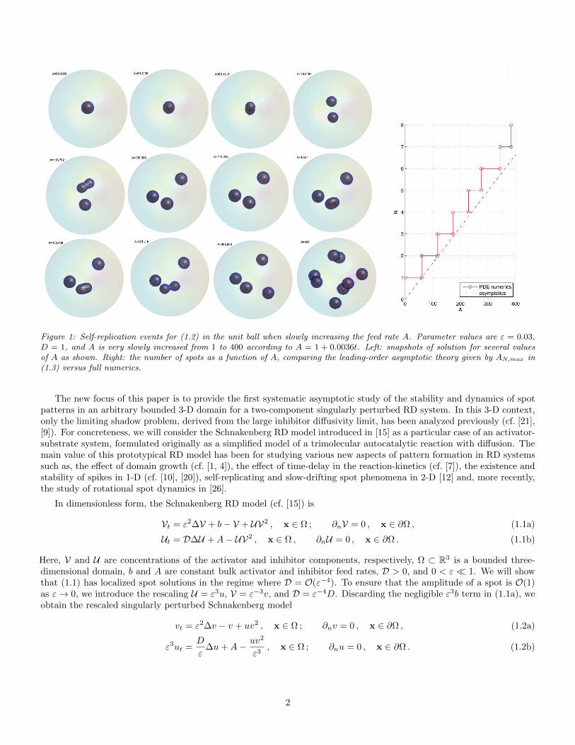
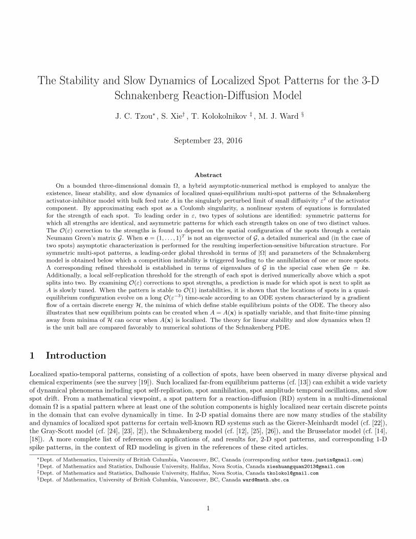
Figure 1: Self-replication events for (1.2) in the unit ball when slowly increasing the feed rate A. Parameter values are ε = 0.03,D = 1, and A is very slowly increased from 1 to 400 according to A = 1 + 0.0036t. Left: snapshots of solution for several valuesof A as shown. Right: the number of spots as a function of A, comparing the leading-order asymptotic theory given by AN,max in(1.3) versus full numerics.

The new focus of this paper is to provide the first systematic asymptotic study of the stability and dynamics of spotpatterns in an arbitrary bounded 3-D domain for a two-component singularly perturbed RD system. In this 3-D context,only the limiting shadow problem, derived from the large inhibitor diffusivity limit, has been analyzed previously (cf. [21],[9]). For concreteness, we will consider the Schnakenberg RD model introduced in [15] as a particular case of an activator-substrate system, formulated originally as a simplified model of a trimolecular autocatalytic reaction with diffusion. Themain value of this prototypical RD model has been for studying various new aspects of pattern formation in RD systemssuch as, the effect of domain growth (cf. [1, 4]), the effect of time-delay in the reaction-kinetics (cf. [7]), the existence andstability of spikes in 1-D (cf. [10], [20]), self-replicating and slow-drifting spot phenomena in 2-D [12] and, more recently,the study of rotational spot dynamics in [26].

In dimensionless form, the Schnakenberg RD model (cf. [15]) is

Vt = ε2∆V + b− V + UV2 , x ∈ Ω ; ∂nV = 0 , x ∈ ∂Ω , (1.1a)

Ut = D∆U +A− UV2 , x ∈ Ω , ∂nU = 0 , x ∈ ∂Ω . (1.1b)

Here, V and U are concentrations of the activator and inhibitor components, respectively, Ω ⊂ R3 is a bounded three-dimensional domain, b and A are constant bulk activator and inhibitor feed rates, D > 0, and 0 < ε 1. We will showthat (1.1) has localized spot solutions in the regime where D = O(ε−4). To ensure that the amplitude of a spot is O(1)as ε→ 0, we introduce the rescaling U = ε3u, V = ε−3v, and D = ε−4D. Discarding the negligible ε3b term in (1.1a), weobtain the rescaled singularly perturbed Schnakenberg model

vt = ε2∆v − v + uv2 , x ∈ Ω ; ∂nv = 0 , x ∈ ∂Ω , (1.2a)

ε3ut =D

ε∆u+A− uv2

ε3, x ∈ Ω ; ∂nu = 0 , x ∈ ∂Ω . (1.2b)

2

Figure 2: Coarsening when decreasing the feed rate A. Parameter values are ε = 0.03, D = 1, and A is very slowly decreased from400 to 1 according to A = 400− 0.0036t. Left: snapshots of solution for several values of A as shown. Right: the number of spotsas a function of A: leading-order asymptotic theory given by AN,min in (1.3) versus full numerics.

The goal of this paper is to develop a hybrid asymptotic-numerical approach to analyze the existence, linear stability,and slow dynamics of quasi-equilibrium N -spot patterns for the 3-D RD model (1.2) in the limit ε → 0. By using aformal asymptotic analysis, in §2 an N -spot quasi-equilibrium pattern is constructed for (1.2) when A > 0 is constant byasymptotically matching a local approximation of the solution near each spot to a global representation of the solutiondefined in terms of the Neumann Green’s function of the Laplacian. The local problem near each spot, referred to asthe core problem, is a simple radially-symmetric BVP system that must be solved numerically. In the global, or outer,representation of the solution, each spot at a given instant in time is asymptotically approximated by a 3-D Coulombsingularity for u of strength Sj at location xj ∈ Ω for j = 1, . . . , N . We show that to within O(ε) terms, there are“symmetric” spot quasi-equilibria for which the source strengths Sj are given by Sj = Sc +O(ε) for j = 1, . . . , N , where

the common value Sc ≡ A|Ω|/(4πN√D), is independent of the spatial configuration of the spots in the domain. The

O(ε) correction terms to the source strengths do, however, depend on the spot locations through a Neumann Green’smatrix G. In contrast, for the 2-D quasi-equilibrium spot patterns constructed in [12], [2], [14] and [18], it was foundthat the O(ε) deviation in a common value for the source-strengths is replaced by a much larger O(ν) correction, whereν ≡ −1/ log ε. As a result, unless ε is extremely small, in a 2-D domain the source strengths for localized spot patternsare rather strongly coupled, and do depend significantly on the overall spatial configuration of the spots.

In §2.1 we show that, to leading-order in ε, there are also branches of “asymmetric” N -spot quasi-equilibria for whichthe source strengths have two distinctly different values. To leading-order in ε, these asymmetric quasi-equilibria allbifurcate from the symmetric solution branch at a common bifurcation point S = Scf ≈ 4.52. Upon including the O(ε)terms, we find that this common bifurcation point structure for the asymmetric quasi-equilibria persists only for spotconfigurations x1, . . .xN for which e = (1, . . . , 1)T is an eigenvector of the Neumann Green’s matrix G. In the unit ballsuch special spot configurations occur when spots are located at vertices of a platonic solid concentric within the ball,when spots are equally-spaced along an equator concentric within the ball, and for many of the equilibrium configurationsof the ODE system for slow spot dynamics derived below in §4. When e is not an eigenvector of G, we show that there isan intricate imperfection-sensitive bifurcation structure of asymmetric quasi-equilibria for S near Scf . For the case where

3

N = 2, we provide a detailed analytical characterization of this imperfection-sensitive bifurcation behavior. We remarkthat a similar imperfection sensitivity behavior for 2-D quasi-equilibrium spot patterns was first identified numerically in[18] for the Brusselator RD model, but no explicit asymptotic analysis of this behavior was given. Imperfection-sensitivitybehavior, and the specific role of whether or not e is an eigenvector of a certain Green’s matrix, was not identified in theearlier analyses of [22], [25], [24], [23], [12], [2], and [14] of 2-D spot patterns for other RD models.

In §3 we analyze the linear stability of N -spot symmetric quasi-equilibrium solutions to two distinct types of O(1)time-scale instabilities. From a numerical study of a local eigenvalue problem near each spot, associated with locallynon-radial perturbations, in §3.2 we show that the dominant spot shape-deforming instability is a mode l = 2 sphericalharmonic, which we refer to as a peanut-splitting instability. This linear instability occurs when a spot source-strengthincreases above the threshold Σ2 ≈ 20.16. We then verify numerically that this linear instability mechanism triggers anonlinear spot self-replication event. In addition, for N ≥ 2, a formal asymptotic analysis is used to derive an eigenvalueproblem associated with locally radially symmetric perturbations near each spot. To leading-order as ε→ 0 we show thatthis linear competition instability, which preserves the sum of the spot amplitudes, is triggered through a zero-eigenvaluecrossing when the common source strength Sc decreases below the threshold Scf ≈ 4.52, the common bifurcation point ofasymmetric quasi-equilibria in the leading-order theory. This linear instability is found numerically to be the trigger ofspot annihilation events. In summary, since Sj = Sc+O(ε) for j = 1, . . . , N , our leading-order asymptotic theory predictsthat symmetric quasi-equilibrium N -spot patterns for N ≥ 2 are linearly stable on an O(1) time-scale if and only if

AN,min < A < AN,max, AN,min ≡ 56.798N√D/|Ω|, AN,max ≡ 253.33N

√D/|Ω|. (1.3)

Spot self-replication event is triggered when the feed A is increased above the threshold AN,max and spot annihilationevent due to overcrowding is triggered when A is decreased below AN,min.

Our hybrid analytical-numerical theory for the existence and linear stability of quasi-equilibrium patterns is validatedfor the unit ball with rather extensive full numerical simulations of the 3-D PDE system (1.2) using the finite-elementpackage FlexPDE6 [6]. For the unit ball, the Neumann Green’s function is known analytically (cf. [3]), making thecomparison convenient. Because FlexPDE6 dynamically adapts the mesh according to the evolution of the solution, it isparticularly useful for computing localized solutions in 3-D. In our computations, FlexPDE6 used up to 40000 nodes withε = 0.03.

Figure 1 illustrates the spot splitting phenomenon. Here, the feed rate A is ramped up very slowly, resulting insuccessive spot-replication events. The first such event occurs at around A ≈ 60, in excellent agreement with thetheoretical prediction A1,max = 60.48. More generally, the asymptotic curve AN,max is in excellent agreement with thenumerics for a wide range of A, see Figure 1 (right).

The overcrowding instability is illustrated in Figure 2, where the feed rate A is ramped down very slowly, and the spotsare eliminated one-by-one due to the competition instability. Again, good agreement between numerics and asymptoticsis observed, as shown in Figure 2 (right), especially for small numbers of spots. For example the theory predicts thattwo spots become unstable as A is decreased below A2,min = 27.1, whereas full numerics show that one of the two spotsdisappears at around A ≈ 28.

For the special case where e is an eigenvector of the Neumann Green’s matrix G, in Main Result 3.1 we establish amore refined asymptotic prediction for the competition instability threshold that involves the smallest eigenvalue of G inthe subspace orthogonal to e. In addition, in §3.1 we formulate the linear stability problem for asymmetric quasi-equilibriaand give some partial results for their stability.

When the stability condition (1.3) on the source strengths holds, in §4 we show that the spot locations associated withan N -spot symmetric quasi-equilibrium evolves to a true steady-state configuration over a long O(ε−3) time-scale. Toleading order in ε, in (4.18) of Main Result 4.2 we show that the slow spot dynamics satisfy an ODE system defined bya gradient flow of a certain discrete energy H(x1, . . . ,xN ), which involves the Neumann Green’s function and its regularpart. Minima of this discrete energy are stable equilibrium points of this limiting ODE spot dynamics, and we explicitlyidentify certain such equilibrium spot configurations. A higher-order analysis, leading to the ODE dynamics (4.13) coupledto the constraints (2.34), shows that the slow spot dynamics consists of a weakly coupled differential algebraic system(DAE) of ODEs, in which the spot source strengths depend only weakly as ε→ 0 on the spot locations.

In comparison, in a 2-D setting, the dynamical characterization of slow spot dynamics consists of a DAE system thatcouples ODEs for the spot locations to a nonlinear algebraic system for the spot source strengths defined in terms ofa Green’s matrix, which depends on the overall spot configuration (cf. [12], [2], [18]). This DAE system of slow spot

4

dynamics in 2-D is rather strongly coupled, owing to the logarithmic gauge ν = O (−1/ log ε). As a result of this strongcoupling in 2-D, spot self-replication events can be triggered intrinsically during the slow dynamics of a collection of spotswhenever a particular spot source strength exceeds a critical value (cf. [12], [2], [14]). In contrast, in our 3-D setting wherethe spots have an asymptotically common source strength, with an error of only O(ε), such intrinsically triggered spotself-replication events do not typically occur for ε small. Instead, in 3-D an external parameter such as the feed-rate, orthe domain volume, needs to be increased dynamically in order to trigger spot self-replication events.

In §4.1 we extend our asymptotic theory for constant A to the case of a spatially variable feed, where A = A(x) in(1.2b). For the linear stability theory, we find that the leading-order result (1.3) still holds provided that we replace A in(1.3) with A, which denotes the spatial average of A(x) over the domain. Moreover, to leading order in ε, the slow spotdynamics is characterized in Main Result 4.3 in terms of the discrete energy H and an additional nonlocal term involvingA(x). In the unit ball, our ODEs characterizing slow spot dynamics are verified with full numerical FlexPDE6 simulationsof (1.2). For a few specific choices of the variable feed-rate, we illustrate from our ODEs, and from full numerical PDEsimulations, the effect of spot pinning, whereby a spot trajectory can be pinned to a new equilibrium state created by thenon-uniform feed-rate. Finally, in §5 we suggest a few open problems that warrant further study.

2 N-Spot Quasi-Equilibria

In this section, we use the method of matched asymptotic expansions to construct an N -spot quasi-equilibrium solutionto (1.2). In our analysis below we assume that the feed A > 0 in (1.2b) is constant. The case of the spatially variable feedA(x) > 0 is considered in §4.1. We construct a pattern for which the spot solution is, to a first approximation, locallyradially symmetric in an O(ε) region near the centers x1, . . . ,xN of the spots, where we assume |xi−xj | = O(1) for i 6= j.On an O(1) time-scale, we construct a quasi-equilibrium solution where the spot locations are, for ε → 0, stationary intime. In §4, we will show that the spot dynamics is slow and occurs on the long time-scale t = O(ε−3) 1.

In the inner region near the j-th spot, we introduce the local variables

y = ε−1(x− xj) , v(xj + εy) =√D [Vj0(ρ) + εVj1 + · · · ] , u(xj + εy) =

1√D

[Uj0(ρ) + εUj1 + · · · ] , (2.1)

where ρ = |y|. Upon substituting (2.1) into (1.2) we obtain, to leading order on 0 < ρ <∞, that

∆ρVj0 − Vj0 + Uj0V2j0 = 0 , V ′j0(0) = 0 , Vj0 → 0 , as ρ→∞ , (2.2a)

∆ρUj0 − Uj0V 2j0 = 0 , U ′j(0) = 0 , (2.2b)

where ∆ρVj0 ≡ V ′′j0 + 2ρ−1V ′j0. The linear −Vj0 term in (2.2a) allows us to impose an exponential decay condition atinfinity for Vj0, whereas the far-field behavior of Uj0 must be proportional to the free-space Green’s function for theLaplacian in 3-D. As such, in terms of some unknown source strength Sj , we impose limρ0→∞

∫ ρ00ρ2∂ρUj0 dρ = Sj , so

that the far-field behavior for Uj0 isUj0 ∼ µj − Sj/ρ+ · · · , as ρ→∞ , (2.2c)

where µj = µ0(Sj) must be computed numerically from (2.2). From (2.2b), we readily obtain the identity

Sj =

∫ ∞

0

Uj0V2j0 ρ

2 dρ . (2.3)

Next, we obtain an asymptotic solution for u in the outer region in terms of the Neumann Green’s function. We firstnote that v ∼ 0 in the outer region, and that from (2.1) and (2.3) we can express the term ε−3uv2 in (1.2b) in the senseof distributions as

ε−3uv2 → 4π√D

N∑

j=1

(∫ ∞

0

Uj0V2j0ρ

2 dρ

)δ(x− xj) = 4π

√D

N∑

j=1

Sjδ(x− xj) . (2.4)

Therefore, from (1.2b), the quasi-equilibrium solution for u in the outer region satisfies

1

ε∆u+

A

D∼ 4π√

D

N∑

j=1

Sjδ(x− xj) , x ∈ Ω ; ∂nu = 0 , x ∈ ∂Ω . (2.5)

5

This expression suggests an expansion for u in the form

u ∼ u0 + εu1 + ε2u2 + · · · , (2.6)

where u0 is an unknown global constant, and where u1 satisfies

∆u1 +A

D=

4π√D

N∑

j=1

Sjδ(x− xj) , x ∈ Ω ; ∂nu1 = 0 , x ∈ ∂Ω . (2.7)

By applying the divergence theorem to (2.7), we obtain the solvability condition

N∑

j=1

Sj =A|Ω|

4π√D. (2.8)

Then, we write the solution to (2.7) as

u1 = − 4π√D

N∑

i=1

SiG(x; xi) + u1 , (2.9)

for some unknown constant u1, where G(x, ξ) is the unique Neumann Green’s function satisfying

∆G =1

|Ω| − δ(x− ξ) , x ∈ Ω ; ∂nG = 0 , x ∈ ∂Ω , (2.10a)

G(x; ξ) =1

4π|x− ξ| +R(x; ξ) , as x→ ξ ;

∫

Ω

Gdx = 0 , (2.10b)

where R(x; ξ) is smooth. In (2.10b), R(ξ; ξ) is called the regular part of G at the singularity x = ξ. For the special casewhere Ω is the unit ball, the Neumann Green’s function is given explicitly by (cf. [3])

G(x; ξ) =1

4π|x− ξ| +1

4π|x||x′ − ξ| +1

4πlog

(2

1− x·ξ + |x||x′ − ξ|

)+

1

8π

(|x|2 + |ξ|2

)− 7

10π. (2.11a)

Here x′ = x/|x|2 is the image point to x outside the unit ball, and · denotes the dot product. To calculate R(ξ; ξ) from(2.11a) we take the limit of G(x, ξ) as x → ξ and extract the nonsingular part of the resulting expression. We readilyobtain that

R(ξ; ξ) =1

4π (1− |ξ|2)− 1

4πlog(1− |ξ|2

)+|ξ|24π− 7

10π. (2.11b)

Next, by using (2.6) with (2.9) and (2.10b), we obtain that the local behavior of u near xj is

u ∼ u0 + ε

− Sj√

D|x− xj |− 4π√

D

SjRjj +

N∑

i=1

i 6=j

SiGji

+ u1

, as x→ xj . (2.12)

Here, we have defined Rjj ≡ R(xj ; xj), and Gji ≡ G(xj ; xi). Matching the local behavior (2.12) to the far-field behavior(2.2c) of the inner solution Uj0, we find to leading order that

µj =√Du0 , j = 1, . . . , N , (2.13)

while the singularity behavior matches by construction. Because the spot strengths are determined in terms of µj , thesimplest N -spot pattern is one in which all spots have a common source strength Sj = Sc for j = 1, . . . , N , independentof their locations. From (2.8), we obtain that this common source strength is

Sc =A|Ω|

4πN√D. (2.14)

6

We refer to such a pattern as a “symmetric” pattern. This result is analogous to that for the mean first passage time(MFPT) for a narrow capture problem in a three-dimensional domain with N small identical traps [3], where the leading-order average MFPT is independent of the locations of the traps in the domain.

A symmetric quasi-equilibrium pattern of N spots is then characterized to leading-order by

vqe ∼√D

N∑

i=1

Vc(ε−1|x− xi|

), uqe ∼

1√Dµ0 + ε

(−4πSc√

D

N∑

i=1

G(x; xi) + u1

), (2.15)

where u1 is a constant to be determined below in §2.1 by a higher order matching procedure. Here Vc(ρ) and µ0 = µ0(S),with S = Sc, are determined by the following radially symmetric core problem on 0 < ρ <∞:

∆ρVc − Vc + UcV2c = 0 , V ′c (0) = 0 , Vc → 0 , as ρ→∞ , (2.16a)

∆ρUc − UcV 2c = 0 , U ′c(0) = 0 , Uc ∼ µ0 −

S

ρ, as ρ→∞ . (2.16b)

In the inner region near xj , we have that vqe and uqe are given to leading order by

vqe ∼√DVc

(ε−1|x− xj |

), uqe ∼

1√DUc(ε−1|x− xj |

). (2.17)

Upon solving the BVP (2.16) using numerical continuation, we plot µ0 in terms of the strength S in Fig. 3(a). The foldpoint at (Scf , µ0f ) ≈ (4.52, 5.78) divides µ0(S) into a left and right branch as shown in Fig. 3(a). In addition, in Fig. 3(b)and Fig. 3(c) we plot Vc and Uc versus ρ, respectively, for a few values of S. We observe from Fig. 3(b) that Vc has avolcano-shaped profile, characterized by a maximum not at ρ = 0, when S ≥ 18.7.

0 5 10 15 20 25 30 35S

5

6

7

8

9

10

11

µ0

(a) µ0 versus S

0 5 10 15ρ

0

0.2

0.4

0.6

0.8

1

Vc

(b) Vc versus ρ

0 5 10 15ρ

1

2

3

4

5

6

7

8

Uc

(c) Uc versus ρ

Figure 3: In (a), we plot the relationship µ0 = µ0(S) as obtained from a numerical solution of the core problem (2.16). The foldpoint at (Scf , µ0f ) ≈ (4.52, 5.78) divides µ0(S) into a left and right branch. In (b), we plot Vc versus ρ = |y| for S = 3.67 (dotted),S = 18.7 (dashed), and S = 29.1 (solid). For S & 18.7, the profile is volcano-shaped so that the maximum of Vc occurs at ρ > 0.When S . 18.7, the maximum of Vc is at ρ = 0. In (c), we show the corresponding profiles for Uc(ρ).

We can determine the limiting asymptotics as S → 0 for the curve µ0(S) by seeking a perturbation solution of (2.16)as S → 0. We readily derive for S → 0 that

Uc ∼b

S

(1 +

S2

b2(µ1 + Uc1) + · · ·

), Vc ∼

S

b

(w +

S2

b2(−µ1w + Vc1)

), (2.18)

and that µ0(S) for S 1 has the limiting asymptotics

µ0 ∼b

S

(1 +

S2

b2µ1 + · · ·

); b ≡

∫ ∞

0

ρ2w2 dρ , µ1 ≡ b−1

∫ ∞

0

ρ2Vc1 dρ . (2.19)

7

0 5 10 15 20S

6

8

10

12

14

16

µ0

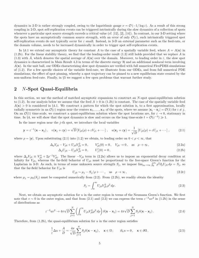
Figure 4: Comparison of the asymptotic result (2.19) for µ0 for small S (discrete points) with the numerical result (solid curve)computed from (2.16). In (2.19) we use b ≈ 10.43 and µ1 ≈ 10.67. The asymptotic result agrees well on 0 < S < 3, with theminimum of the µ0 versus S graph occurring at Scf ≈ 4.52.

Here w(ρ) is the unique ground-state solution of ∆ρw − w + w2 = 0 with w(0) > 0 and limρ→∞ w = 0, while Uc1(ρ) andVc1(ρ) are the unique solutions on 0 < ρ <∞ to

LVc1 ≡ ∆ρVc1 − Vc1 + 2wVc1 = −w2Uc1 ; V ′c1(0) = 0 , limρ→∞

Vc1 = 0 , (2.20a)

∆ρUc1 = w2 ; U ′c1(0) = 0 , Uc1 ∼ −b/ρ , as ρ→∞ . (2.20b)

By solving for w and the pair (Uc1, Vc1) numerically we estimate that b ≈ 10.43 and µ1 ≈ 10.67. In Fig. 4 we show thatthe asymptotic result (2.19) agrees very closely with the corresponding numerical result for most of the left branch of theµ0 versus S curve of Fig. 3(a).

For a given µ0 > µ0f , the multi-valued nature of S(µ0) in Fig. 3(a) gives rise to the possibility of “asymmetric”patterns consisting of N` spots with strength S` on the left branch and Nr spots with strength Sr on the right branch.Such a pattern takes the form

vqe ∼√D

N∑

i=1

Vc`(ε−1|x− xi|

)+√D

Nr∑

i=1

Vcr(ε−1|x− xi|

), (2.21a)

uqe ∼µ0√D

+ ε

(−4πS`√

D

N∑

i=1

G(x; xi)−4πSr√D

Nr∑

i=1

G(x; xi) + u1

), (2.21b)

where the pairs (Vc`, Uc`) and (Vcr, Ucr) are the solutions to (2.16) with Uc` ∼ µ0 − S`/ρ as ρ→∞, and Ucr ∼ µ0 − Sr/ρas ρ → ∞, respectively. For given positive integers N` and Nr, with N = N` + Nr, the two source strengths S` and Srfor the leading-order asymmetric pattern must be determined from the nonlinear algebraic problem

N`S` +NrSr =A|Ω|

4π√D, µ0(S`) = µ0(Sr) , where S` < Scf < Sr . (2.22)

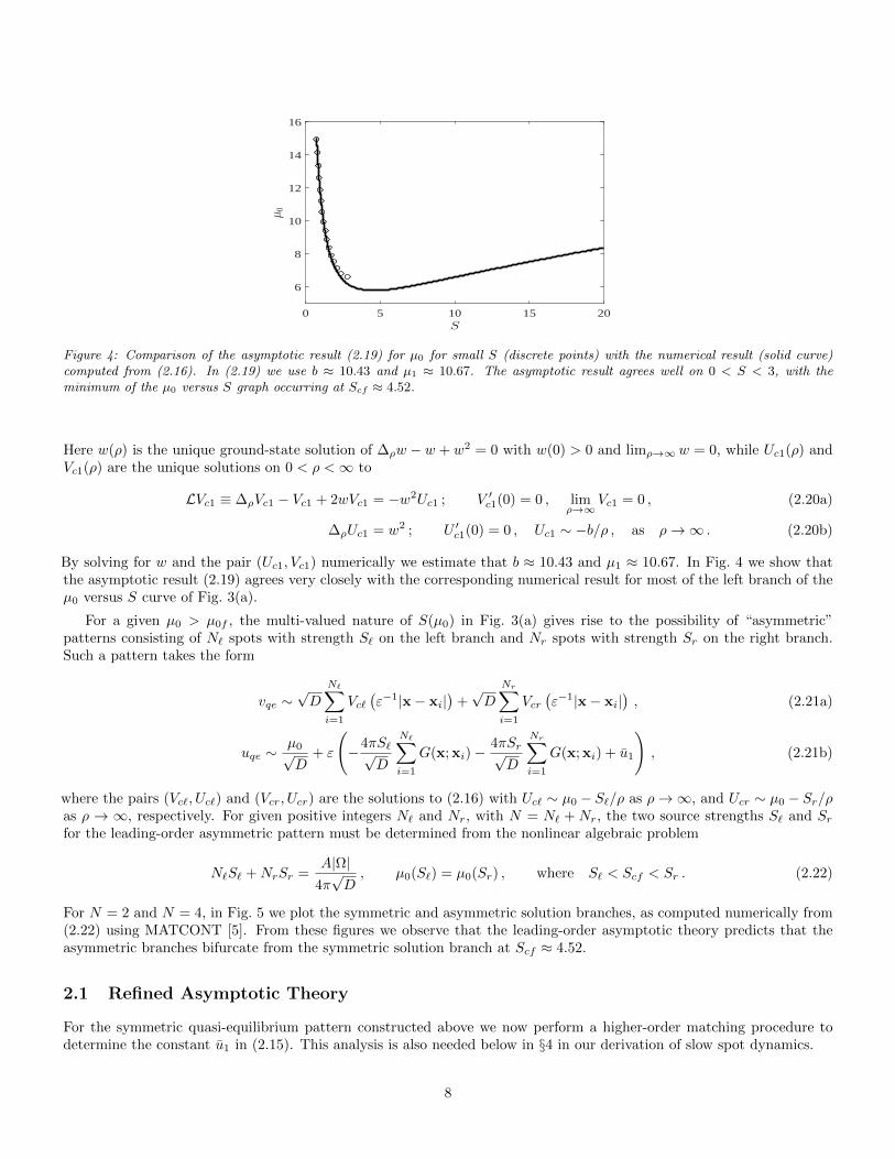
For N = 2 and N = 4, in Fig. 5 we plot the symmetric and asymmetric solution branches, as computed numerically from(2.22) using MATCONT [5]. From these figures we observe that the leading-order asymptotic theory predicts that theasymmetric branches bifurcate from the symmetric solution branch at Scf ≈ 4.52.

2.1 Refined Asymptotic Theory

For the symmetric quasi-equilibrium pattern constructed above we now perform a higher-order matching procedure todetermine the constant u1 in (2.15). This analysis is also needed below in §4 in our derivation of slow spot dynamics.

8

3 4 5 6 73

4

5

6

7

8

9

A|Ω|/(4πN√D)

√1 N

∑S

2 j

3 4 5 6 73

4

5

6

7

8

9

10

11

12

A|Ω|/(4πN√D)

√1 N

∑S

2 j

Figure 5: Bifurcation diagram of√N−1

∑i S

2iε versus A|Ω|/(4πN

√D) computed using MATCONT [5] from the leading-order

problem (2.22) for D = 0.1 and ε = 0.05 for N = 2 spots (left panel) and for N = 4 spots (right panel). The heavy solid curves arethe symmetric solution branch. In the left panel, the dashed curve represents the asymmetric branch. In the right panel the labellingof the curves is: (dashed curve) Nr = 3 and N` = 1; (dashed-dotted curve) Nr = N` = 2; (dotted curve) Nr = 1 and N` = 3. Theleading-order theory predicts that the asymmetric branches bifurcate from a common point.

With u0 = µ0/√D and S = Sc, we first write the local behavior (2.12) in terms of inner variables as

u ∼ 1√D

(µ0 −

Scρ

)+ ε

[−4πSc√

D(Ge)j + u1

]+ · · · , as x→ xj . (2.23)

Here e ≡ (1, . . . , 1)T , while G is the N ×N symmetric Neumann Green’s matrix with matrix entries (G)ij = G(xj ; xi) fori 6= j and (G)jj = R(xj ; xj).

To account for the O(ε) correction to the singularity behavior in (2.23), we need the higher-order terms Uj1 andVj1 in the inner expansion as introduced in (2.1). Upon substituting (2.1) into (1.2), we obtain in matrix form thatW1 = (Vj1, Uj1)T satisfies

∆ρW1 +MW1 = 0 , 0 < ρ <∞ , (2.24a)

W′1(0) = (0, 0)T ; W1 ∼ (0, αj)

T , as ρ→∞ , (2.24b)

where αj and the 2× 2 matrix M are defined by

αj ≡ −4πSc (Ge)j + u1

√D , M≡

(−1 + 2UcVc V 2

c

−2UcVc −V 2c

). (2.24c)

We can readily identify the solution to (2.24) by differentiating the core problem (2.16) with respect to S. For S 6= Scf ,we obtain that

Vj1 =αj

µ′0(S)∂SVc , Uj1 =

αjµ′0(S)

∂SUc . (2.25)

Therefore, provided that Sc 6= Scf , we have for S = Sc that

Uj1 ∼ αj −αj

µ′0(Sc)ρ, as ρ→∞ ; and

∫ ∞

0

(2UcVcVj1 + V 2

c Uj1)ρ2 dρ =

αjµ′0(Sc)

. (2.26)

Next, we proceed to one higher order in the outer region. In the sense of distributions, and upon using the integralidentity in (2.26), we get as ε→ 0 that

ε−3uv2 → 4π√D

N∑

j=1

[Sc +

εαjµ′0(Sc)

]δ(x− xj) . (2.27)

9

0 0.05 0.1 0.15 0.2ε

10

12

14

16

18

20

22

uqe| r=

1

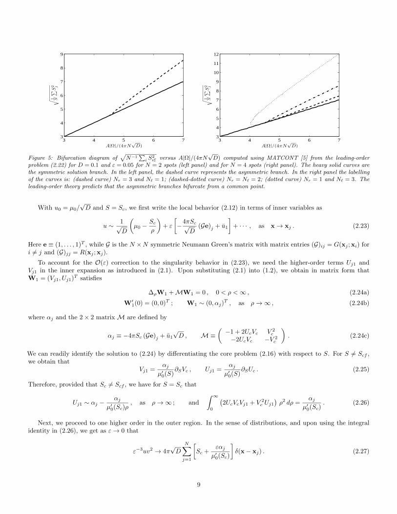
Figure 6: Comparison of asymptotic result (2.31) (solid curve) and full numerical result computed from the steady-state of (1.2)(discrete points) for u corresponding to a one-spot solution centered at the origin in the unit ball. The parameters are A = 10 andD = 0.1.

By using (2.27) in (1.2b), we obtain that the term u2 in the outer expansion (2.6) satisfies

∆u2 =4π√

Dµ′0(Sc)

N∑

j=1

αjδ(x− xj) , x ∈ Ω ; ∂nu2 = 0 , x ∈ ∂Ω . (2.28)

The solvability condition for (2.28) is that∑Nj=1 αj = 0. Upon using (2.24c) for αj , we determine u1 as

u1 =4πSc

N√D

(eTGe

). (2.29)

Then, by solving (2.28) for u2 up to a constant, and by using (2.15) and (2.29), we obtain that the outer expansion for asymmetric N -spot quasi-equilibrium solution is

uqe ∼µ0√D

+4πεSc√D

(−

N∑

i=1

G(x; xi) +eTGe

N

)− 4πε2

√D

(4πScµ′0(Sc)

) N∑

i=1

[eTGe

N− (Ge)i

]G(x; xi) + ε2u2 + · · · . (2.30)

To illustrate (2.30), we let N = 1, Ω be the unit ball, and take x1 = 0, so that the spot is at the center of the ball.Then, we use the explicit Green’s function (2.11) to obtain from (2.30) that

uqe ∼µ0√D− εSc√

D

(r2

2+

1

r

)+O(ε2) , Sc =

A

3√D,

where r = |x|, so that on the domain boundary where r = 1 we get

uqe =µ0√D− 3εSc

2√D, x ∈ ∂Ω . (2.31)

For this radially symmetric setting, we can solve for the steady-state of (1.2) numerically and then compare with theasymptotic result (2.31). The comparison of uqe on the domain boundary versus ε in Fig. 6 shows that the asymptoticresult is very accurate even when ε is only moderately small.

Finally, we provide an alternative analysis to construct an N -spot quasi-equilibrium solution, which is needed in §3and §4 below. In this approach, we allow the source strength Sj in (2.2c) to depend weakly on ε, and so we write Ujε,Vjε to be the solution to (2.2) for which Ujε ∼ µj − Sjε/ρ as ρ→∞, where µj ≡ µ0(Sjε). By proceeding as in (2.4) and(2.5), we obtain that the outer solution satisfies

∆u+εA

D∼ 4πε√

D

N∑

j=1

Sjεδ(x− xj) , x ∈ Ω ; ∂nu = 0 , x ∈ ∂Ω . (2.32)

10

Instead of expanding u as a power series in ε as in (2.6), we solve (2.32) exactly to obtain

u = ξ − 4πε√D

N∑

i=1

SiεG(x; xi) ,

N∑

i=1

Siε =A|Ω|

4π√D, (2.33)

where ξ is a constant and G satisfies (2.10). By matching the local behavior of the outer solution u as x → xj with thefar field behavior uj = D−1/2Ujε ∼ D−1/2 (µj − Sjε/ρ) of the j-th inner solution, where µj ≡ µ0(Sjε), we obtain thatSjε for j = 1, . . . , N and the constant ξ must satisfy the N + 1 dimensional weakly coupled nonlinear algebraic system

ξ − 4πε√D

(GS)j =µ0(Sjε)√

D, j = 1, . . . , N ;

N∑

j=1

Sjε =A|Ω|

4π√D. (2.34)

Here µ0(Sjε) is to be computed from the core problem (2.2), S ≡ (S1ε, . . . , SNε)T , and G is the symmetric NeumannGreen’s matrix with matrix entries (G)ij = G(xj ; xi) for i 6= j and (G)jj = R(xj ; xj). It is readily shown from (2.34) thata two-term expansion for ξ and Sjε is

Sjε ∼ Sc +4πεScµ′0(Sc)

(eTGe

N− (Ge)j

)+ · · · , j = 1, . . . , N ; ξ ∼ µ0(Sc)√

D+

4πε√DN

SceTGe + · · · , (2.35)

provided that Sc 6= Scf . Upon substituting this result into (2.33) we obtain our previous result (2.30) obtained from amore conventional power series representation of the outer solution.

An important special case of (2.34) occurs when the spots locations are aligned so that e = (1, . . . , 1)T is an eigenvectorof the Green’s matrix G. In particular, assume that Ge = k1e for some eigenvalue k1. Then, (2.34) has a solution withS = Sce for any ε > 0, for which

ξ =4πε√DSck1 +

µ0(Sc)√D

, Sc ≡A|Ω|

4πN√D. (2.36)

Therefore, when Ge = k1e, there is a common source-strength solution to (2.34) that is precisely the same as that for theleading-order solution in (2.14). For this special case, we readily identify that that αj = 0 in (2.24c) so that Uj1 = Vj1 = 0from (2.25). As a consequence, we have Ujε = Uc +O(ε2) and Vjε = Vc +O(ε2), which is used below in §3 in our linearstability analysis.

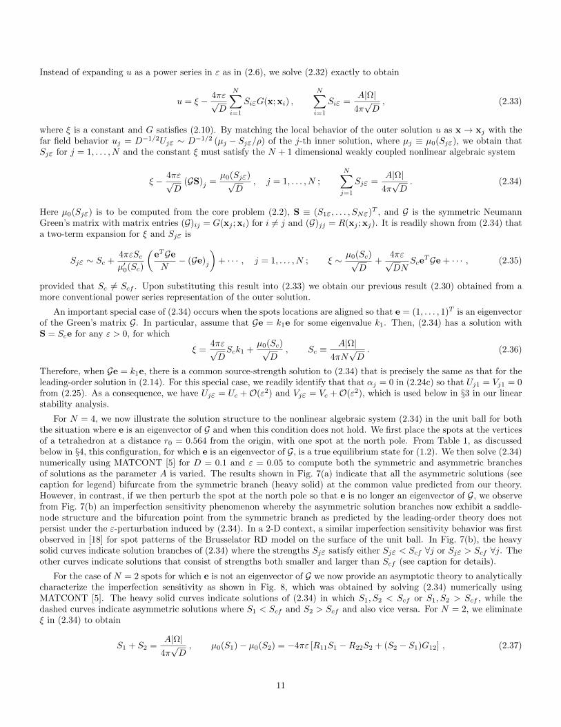
For N = 4, we now illustrate the solution structure to the nonlinear algebraic system (2.34) in the unit ball for boththe situation where e is an eigenvector of G and when this condition does not hold. We first place the spots at the verticesof a tetrahedron at a distance r0 = 0.564 from the origin, with one spot at the north pole. From Table 1, as discussedbelow in §4, this configuration, for which e is an eigenvector of G, is a true equilibrium state for (1.2). We then solve (2.34)numerically using MATCONT [5] for D = 0.1 and ε = 0.05 to compute both the symmetric and asymmetric branchesof solutions as the parameter A is varied. The results shown in Fig. 7(a) indicate that all the asymmetric solutions (seecaption for legend) bifurcate from the symmetric branch (heavy solid) at the common value predicted from our theory.However, in contrast, if we then perturb the spot at the north pole so that e is no longer an eigenvector of G, we observefrom Fig. 7(b) an imperfection sensitivity phenomenon whereby the asymmetric solution branches now exhibit a saddle-node structure and the bifurcation point from the symmetric branch as predicted by the leading-order theory does notpersist under the ε-perturbation induced by (2.34). In a 2-D context, a similar imperfection sensitivity behavior was firstobserved in [18] for spot patterns of the Brusselator RD model on the surface of the unit ball. In Fig. 7(b), the heavysolid curves indicate solution branches of (2.34) where the strengths Sjε satisfy either Sjε < Scf ∀j or Sjε > Scf ∀j. Theother curves indicate solutions that consist of strengths both smaller and larger than Scf (see caption for details).

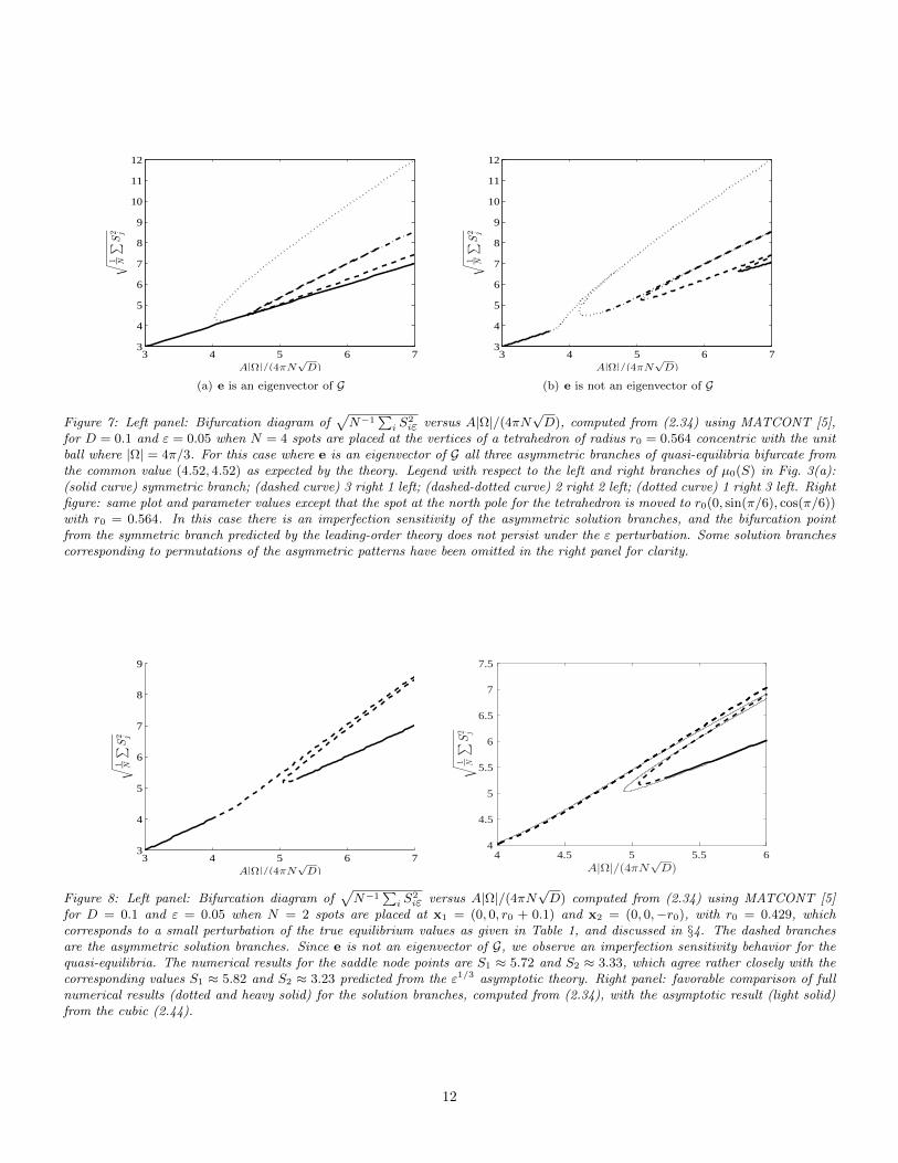
For the case of N = 2 spots for which e is not an eigenvector of G we now provide an asymptotic theory to analyticallycharacterize the imperfection sensitivity as shown in Fig. 8, which was obtained by solving (2.34) numerically usingMATCONT [5]. The heavy solid curves indicate solutions of (2.34) in which S1, S2 < Scf or S1, S2 > Scf , while thedashed curves indicate asymmetric solutions where S1 < Scf and S2 > Scf and also vice versa. For N = 2, we eliminateξ in (2.34) to obtain

S1 + S2 =A|Ω|

4π√D, µ0(S1)− µ0(S2) = −4πε [R11S1 −R22S2 + (S2 − S1)G12] , (2.37)

11

3 4 5 6 73

4

5

6

7

8

9

10

11

12

A|Ω|/(4πN√D)

√1 N

∑S

2 j

(a) e is an eigenvector of G

3 4 5 6 73

4

5

6

7

8

9

10

11

12

A|Ω|/(4πN√D)

√1 N

∑S

2 j

(b) e is not an eigenvector of G

Figure 7: Left panel: Bifurcation diagram of√N−1

∑i S

2iε versus A|Ω|/(4πN

√D), computed from (2.34) using MATCONT [5],

for D = 0.1 and ε = 0.05 when N = 4 spots are placed at the vertices of a tetrahedron of radius r0 = 0.564 concentric with the unitball where |Ω| = 4π/3. For this case where e is an eigenvector of G all three asymmetric branches of quasi-equilibria bifurcate fromthe common value (4.52, 4.52) as expected by the theory. Legend with respect to the left and right branches of µ0(S) in Fig. 3(a):(solid curve) symmetric branch; (dashed curve) 3 right 1 left; (dashed-dotted curve) 2 right 2 left; (dotted curve) 1 right 3 left. Rightfigure: same plot and parameter values except that the spot at the north pole for the tetrahedron is moved to r0(0, sin(π/6), cos(π/6))with r0 = 0.564. In this case there is an imperfection sensitivity of the asymmetric solution branches, and the bifurcation pointfrom the symmetric branch predicted by the leading-order theory does not persist under the ε perturbation. Some solution branchescorresponding to permutations of the asymmetric patterns have been omitted in the right panel for clarity.

3 4 5 6 73

4

5

6

7

8

9

A|Ω|/(4πN√D)

√1 N

∑S

2 j

4 4.5 5 5.5 6A|Ω|/(4πN

√D)

4

4.5

5

5.5

6

6.5

7

7.5

√

1 N

∑

S2 j

Figure 8: Left panel: Bifurcation diagram of√N−1

∑i S

2iε versus A|Ω|/(4πN

√D) computed from (2.34) using MATCONT [5]

for D = 0.1 and ε = 0.05 when N = 2 spots are placed at x1 = (0, 0, r0 + 0.1) and x2 = (0, 0,−r0), with r0 = 0.429, whichcorresponds to a small perturbation of the true equilibrium values as given in Table 1, and discussed in §4. The dashed branchesare the asymmetric solution branches. Since e is not an eigenvector of G, we observe an imperfection sensitivity behavior for thequasi-equilibria. The numerical results for the saddle node points are S1 ≈ 5.72 and S2 ≈ 3.33, which agree rather closely with thecorresponding values S1 ≈ 5.82 and S2 ≈ 3.23 predicted from the ε1/3 asymptotic theory. Right panel: favorable comparison of fullnumerical results (dotted and heavy solid) for the solution branches, computed from (2.34), with the asymptotic result (light solid)from the cubic (2.44).

12

where we have relabeled S1 = S1ε and S2 = S2ε for simplicity. We now introduce a detuning parameter δ that measureshow close we are to the critical value Scf , so that

A|Ω|4π(2)

√D

= Scf +δ

2, δ 1 , (2.38)

and we write S1 and S2 in terms of δ and some S 1 as

S1 = Scf + S +δ

2, S2 = Scf + S − δ

2. (2.39)

Upon substituting (2.39) into (2.37), we obtain using Taylor series, together with µ′0(Scf ) = 0, that

−4πε[Scf (R11 −R22) +O(S, δ)

]= µ′′0(Scf )

(Sδ +O(δ2)

)+µ′′′0 (Scf )

3S3 +O(S2δ, Sδ2, δ3) . (2.40)

To balance the terms in (2.40) we need S = O(ε1/3), and Sδ = O(ε), which yields δ = O(ε2/3). With this scaling, itreadily follows that we can neglect the error terms written in (2.40). We then write S = ε1/3S0 and δ = ε1/3δ0, where S0

satisfies the cubicµ′′′0 (Scf )

3S3

0 + µ′′0(Scf )S0δ0 = −4πScf (R11 −R22) . (2.41)

From the numerical results used for Fig. 3(a), we estimate that µ′′0(Scf ) ≈ 0.15 and µ′′′0 (Scf ) ≈ −0.12. Relabelling thespots so that R11 > R22 without loss of generality, we reduce (2.41) to a canonical cubic by introducing x and y by

S0 = S0dy , δ0 = δ0dx , (2.42a)

where S0d and δ0d are

S0d ≡(

12πScf (R11 −R22)

|µ′′′0 (Scf )|

)1/3

, δ0d ≡( |µ′′′0 (Scf )|

3

)1/3[4πScf (R11 −R22)]

2/3

µ′′0(Scf ), (2.42b)

so that (2.41) reduces to the canonical cubicy3 − xy = 1 . (2.43)

This cubic always has one real solution y3 > 0 for any x, and two additional real solutions y1 and y2, with y1 < ymin ≡−2−1/3 < 0 and ymin < y2 < 0, whenever x > xmin = 2−2/3 + 21/3 ≈ 1.8899.

In summary, in terms of the roots of the cubic (2.43), and the scaling (2.42), the roots of (2.34) near Scf are given interms of x and y by

A|Ω|4π(2)

√D∼ Scf +

(δ0d2

)xε2/3 , (2.44a)

S1 ∼ Scf + ε1/3S0dy +

(δ0d2

)xε2/3 ; S2 ∼ Scf − ε1/3S0dy +

(δ0d2

)xε2/3 . (2.44b)

The saddle-node bifurcation value associated with (2.44) is at

(A|Ω|

4π(2)√D

)

sn

∼ Scf +

(δ0d2

)xminε

2/3 , Scf ≈ 4.52 , xmin ≈ 1.8899 . (2.45)

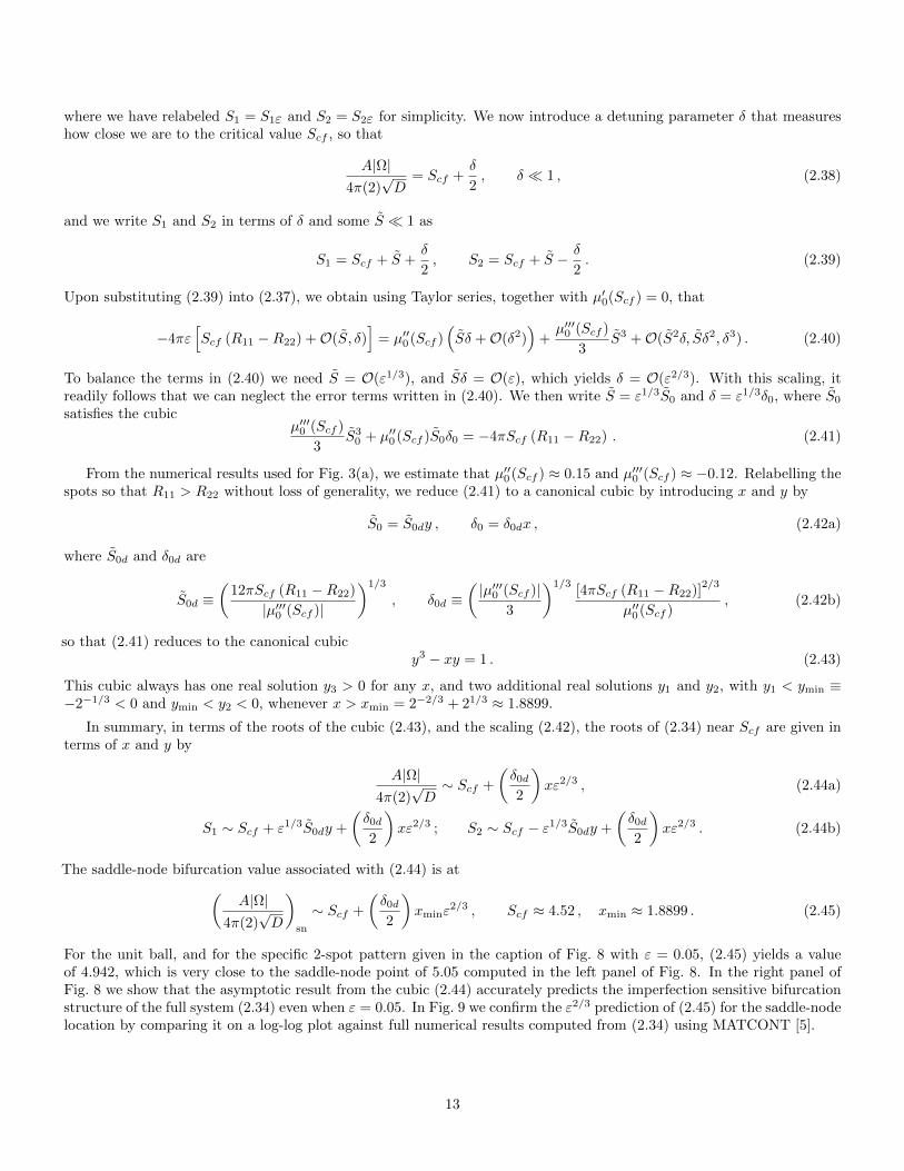
For the unit ball, and for the specific 2-spot pattern given in the caption of Fig. 8 with ε = 0.05, (2.45) yields a valueof 4.942, which is very close to the saddle-node point of 5.05 computed in the left panel of Fig. 8. In the right panel ofFig. 8 we show that the asymptotic result from the cubic (2.44) accurately predicts the imperfection sensitive bifurcationstructure of the full system (2.34) even when ε = 0.05. In Fig. 9 we confirm the ε2/3 prediction of (2.45) for the saddle-nodelocation by comparing it on a log-log plot against full numerical results computed from (2.34) using MATCONT [5].

13

10-6 10-5 10-4 10-3 10-2

ε

10-4

10-3

10-2

10-1

100

(

A|Ω

|4π

(2)√ D

)

sn−Scf

Figure 9: Log-log plot of(

A|Ω|4π(2)

√D

)sn−Scf versus ε characterizing the location of the saddle-node point on the asymmetric solution

branch of Fig. 8 versus ε. The solid curve corresponds to the asymptotic result (2.45), while the discrete points are computed from(2.34) using MATCONT [5]. This plot confirms the ε2/3 scaling law of (2.45).

3 The Linear Stability of Quasi-Equilibrium Patterns

In this section, we analyze the linear stability of symmetric quasi-equilibrium patterns. We begin by considering theeffect of locally radially symmetric perturbations near each spot. We let vqe and uqe denote the N -spot symmetricquasi-equilibrium pattern, and in (1.2) we introduce the perturbation

v = vqe + eλtφ , u = uqe + eλtψ , where |φ| 1, |ψ| 1 , (3.1)

to obtain the linear eigenvalue problem

ε2∆φ− φ+ 2uqevqeφ+ v2qeψ = λφ , x ∈ Ω , ∂nφ = 0 , x ∈ ∂Ω , (3.2a)

D

ε∆ψ − 1

ε3

(2uqevqeφ+ v2

qeψ)

= ε3λψ , x ∈ Ω , ∂nψ = 0 , x ∈ ∂Ω . (3.2b)

In the inner region near the j-th spot at x = xj , we let

φ ∼ cjΦj(ρ) , ψ ∼ cjΨj(ρ)

D, (3.3)

for some constant cj to be determined. We then use the local behavior vqe ∼√DVjε(ρ) and uqe ∼ Ujε(ρ)/

√D to obtain

the leading-order inner eigenvalue problem

∆ρΦj − Φj + 2VjεUjεΦj + V 2jεΨj = λΦj , 0 < ρ <∞ ; Φ′j(0) = 0 , Φj → 0 , as ρ→∞ , (3.4a)

∆ρΨj − 2VjεUjεΦj − V 2jεΨj = 0 , 0 < ρ <∞ ; Ψ′j(0) = 0 . (3.4b)

We will impose the normalization condition that limρ→∞ ρ2∂ρΨj = −1, so that we have the following far-field behaviorin terms of some function Bj = Bj(λ;Sjε):

Ψj ∼1

ρ+Bj(λ;Sjε) , as ρ→∞ . (3.4c)

Here Sjε, for j = 1, . . . , N , is to be determined from the nonlinear algebraic system (2.34). By applying the divergencetheorem to (3.4b), we obtain the integral identity

∫ ∞

0

(2VjεUjεΦj + V 2

jεΨj

)ρ2 dρ = −1 . (3.5)

14

Now in the outer region, the reaction term in (3.2b) of order O(ε−3) is localized. Therefore, in the sense of distributionswe write

ε−3(2uqevqeφ+ v2

qeψ)→ 4π

N∑

j=1

cj

[∫ ∞

0

(2VjεUjεΦj + V 2

jεΨj

)ρ2 dρ

]δ(x− xj) = −4π

N∑

j=1

cjδ(x− xj) ,

so that the outer equation for ψ is

∆ψ = −4πε

D

N∑

i=1

ciδ(x− xi) , x ∈ Ω ; ∂nψ = 0 , x ∈ ∂Ω . (3.6)

The exact solution to (3.6) is

ψ = ψ +4πε

D

N∑

i=1

ciG(x; xi) , (3.7)

where ψ is a constant to be determined, and G(x; xi) is the Neumann Green’s function satisfying (2.10). Then, by applyingthe divergence theorem to (3.6) we obtain the solvability condition

N∑

j=1

cj = 0 . (3.8)

In view of (3.1) and (3.8) we see that the perturbation preserves the sum of the spot amplitudes. As such, this type ofinstability is referred to as a competition instability (c.f. [17]).

Next, we derive a linear algebraic system for the constants cj , j = 1, . . . , N , and ψ. We expand (3.7) as x→ xj and,in terms of inner variables, we get

ψ ∼ ψ +cjDρ

+4πε

D(Gc)j , as x→ xj , (3.9)

where ρ ≡ ε−1|x − xj |, G is the Neumann Green’s matrix, and c ≡ (c1, . . . , cN )T . This local behavior of the outereigenfunction must match with the far-field behavior of the corresponding inner solution, given by ψ ∼ cjD−1 (Bj + 1/ρ)as ρ→∞. In this way, we obtain that c and ψ satisfy

cjBj = Dψ + 4πε (Gc)j , j = 1 , . . . , N ;

N∑

i=1

ci = 0 , (3.10)

where Bj = Bj(λ;Sjε). By eliminating ψ, we readily derive in matrix form that c satisfies the matrix eigenvalue problem

(I − E) (B − 4πεG) c = 0 , E ≡ 1

NeeT ; eT c = 0 , (3.11)

where e = (1, . . . , 1)T , and where B is the diagonal matrix with entries (B)jj = Bj and (B)ij = 0 for i, j = 1, . . . , N . Thediscrete eigenvalues λ of the linearization (3.2) are roots of det ((I − E) (B − 4πεG)) = 0, provided that the correspondingeigenvector c satisfies the side constraint eT c = 0.

We first consider the leading-order theory associated with (3.11). To leading order in ε, we obtain that Sj = Sc+O(ε)for j = 1, . . . , N , where Sc is defined in (2.14), and Ujε ∼ Uc+O(ε) and Vjε ∼ Vc+O(ε), where Uc and Vc satisfy the coreproblem (2.16). As a result, we obtain that B = B(λ;Sc)I +O(ε), where B(λ;Sc) is to be computed from the followingcommon core problem that is the same for each spot:

∆ρΦc − Φc + 2VcUcΦc + V 2c Ψc = λΦc , 0 < ρ <∞ ; Φ′c(0) = 0 , Φc → 0 , as ρ→∞ , (3.12a)

∆ρΨc − 2VcUcΦc − V 2c Ψc = 0 , 0 < ρ <∞ ; Ψ′c(0) = 0 , Ψc ∼

1

ρ+B(λ;Sc) , as ρ→∞ . (3.12b)

For N ≥ 2, the leading-order term in (3.11) yields that the discrete eigenvalues λ of the linearization (3.2) satisfy

B(λ;Sc) = 0 , (3.13)

15

0 5 10 15 20 25 30 35Sc

-1

-0.5

0

0.5

1

1.5

2ℜ(λ)

(a) <(λ) versus Sc

0 5 10 15 20 25 30 35Sc

0

0.05

0.1

0.15

0.2

0.25

0.3

0.35

0.4

ℑ(λ)

(b) =(λ) versus Sc

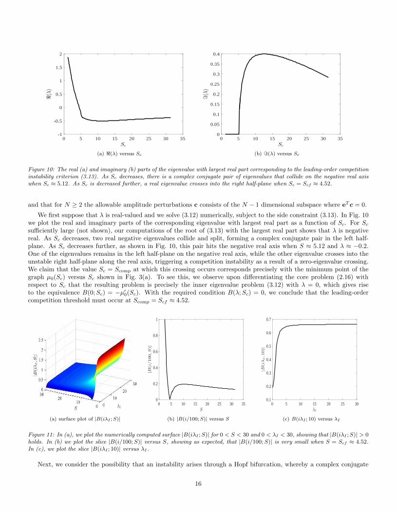
Figure 10: The real (a) and imaginary (b) parts of the eigenvalue with largest real part corresponding to the leading-order competitioninstability criterion (3.13). As Sc decreases, there is a complex conjugate pair of eigenvalues that collide on the negative real axiswhen Sc ≈ 5.12. As Sc is decreased further, a real eigenvalue crosses into the right half-plane when Sc = Scf ≈ 4.52.

and that for N ≥ 2 the allowable amplitude perturbations c consists of the N − 1 dimensional subspace where eT c = 0.

We first suppose that λ is real-valued and we solve (3.12) numerically, subject to the side constraint (3.13). In Fig. 10we plot the real and imaginary parts of the corresponding eigenvalue with largest real part as a function of Sc. For Scsufficiently large (not shown), our computations of the root of (3.13) with the largest real part shows that λ is negativereal. As Sc decreases, two real negative eigenvalues collide and split, forming a complex conjugate pair in the left half-plane. As Sc decreases further, as shown in Fig. 10, this pair hits the negative real axis when S ≈ 5.12 and λ ≈ −0.2.One of the eigenvalues remains in the left half-plane on the negative real axis, while the other eigenvalue crosses into theunstable right half-plane along the real axis, triggering a competition instability as a result of a zero-eigenvalue crossing.We claim that the value Sc = Scomp at which this crossing occurs corresponds precisely with the minimum point of thegraph µ0(Sc) versus Sc shown in Fig. 3(a). To see this, we observe upon differentiating the core problem (2.16) withrespect to Sc that the resulting problem is precisely the inner eigenvalue problem (3.12) with λ = 0, which gives riseto the equivalence B(0;Sc) = −µ′0(Sc). With the required condition B(λ;Sc) = 0, we conclude that the leading-ordercompetition threshold must occur at Scomp = Scf ≈ 4.52.

(a) surface plot of |B(iλI ;S)|

0 5 10 15 20 25 30 35S

0

0.2

0.4

0.6

0.8

1

|B(i/100,S)|

(b) |B(i/100;S)| versus S

0 5 10 15 20 25 30λI

0.1

0.2

0.3

0.4

0.5

0.6

0.7

|B(iλI,10)|

(c) B(iλI ; 10) versus λI

Figure 11: In (a), we plot the numerically computed surface |B(iλI ;S)| for 0 < S < 30 and 0 < λI < 30, showing that |B(iλI ;S)| > 0holds. In (b) we plot the slice |B(i/100;S)| versus S, showing as expected, that |B(i/100;S)| is very small when S = Scf ≈ 4.52.In (c), we plot the slice |B(iλI ; 10)| versus λI .

Next, we consider the possibility that an instability arises through a Hopf bifurcation, whereby a complex conjugate

16

pair of eigenvalues enters <(λ) > 0 through the imaginary axis. We let λ = iλI in (3.12) and, upon separating theresulting system into real and imaginary parts, we readily compute the modulus |B(iλI ;Sc)| numerically as a functionof Sc and λI > 0. The surface plot and slices through the surface shown in Fig. 11 verify that the strict inequality|B(iλI ;Sc)| > 0 holds, and so there can be no Hopf bifurcation as Sc is varied. Since for Sc 1, (3.12) is readily seen toreduce to leading-order to the scalar self-adjoint local eigenvalue problem LΦc0 = λΦc0, where L is defined in (2.20), whichhas no imaginary eigenvalues, it follows by continuity of the eigenvalue path with respect to Sc that any complex-valuedeigenvalues for (3.12), with the side constraint (3.13), must remain in the stable left-half plane <(λ) < 0 for any Sc > 0.

Overall, the numerical results of Fig. 10 and Fig. 11 show that, to leading-order in ε, the N -spot quasi-equilibriumpattern is linearly stable (unstable) to a competition instability when Sc > Scomp (Sc < Scomp). In terms of the parametersA and D, we obtain from (2.14) that, to leading order in ε, a quasi-equilibrium pattern of N identical spots is linearlystable to a competition instability when

A|Ω|4πN

√D> Scomp = Scf ≈ 4.52 . (3.14)

That is, a competition instability is triggered when the total inhibitor feed rate A|Ω| is insufficient to sustain the N spots,or when the interaction of the spots, mediated by the diffusion coefficient D of the inhibitor, is sufficiently strong.

We now make several remarks. First, the leading-order-in-ε linear stability criterion (3.14) is independent of wherethe spots are located. Second, with the competition threshold coinciding with the minimum point of the graph µ0(Sc),the entire left (right) branch of µ0(Sc) is unstable (linearly stable) to a competition instability. Finally, while this leading-order analysis determines when a symmetric quasi-equilibrium pattern loses stability when N ≥ 2, it gives no informationregarding which mode of instability is most dominant. This is unsurprising, since all spots are identical to leading order,regardless of location. A higher order analysis is thus required to determine the dominant mode. We will provide such ahigher order theory below when the spot configuration has a special structure.

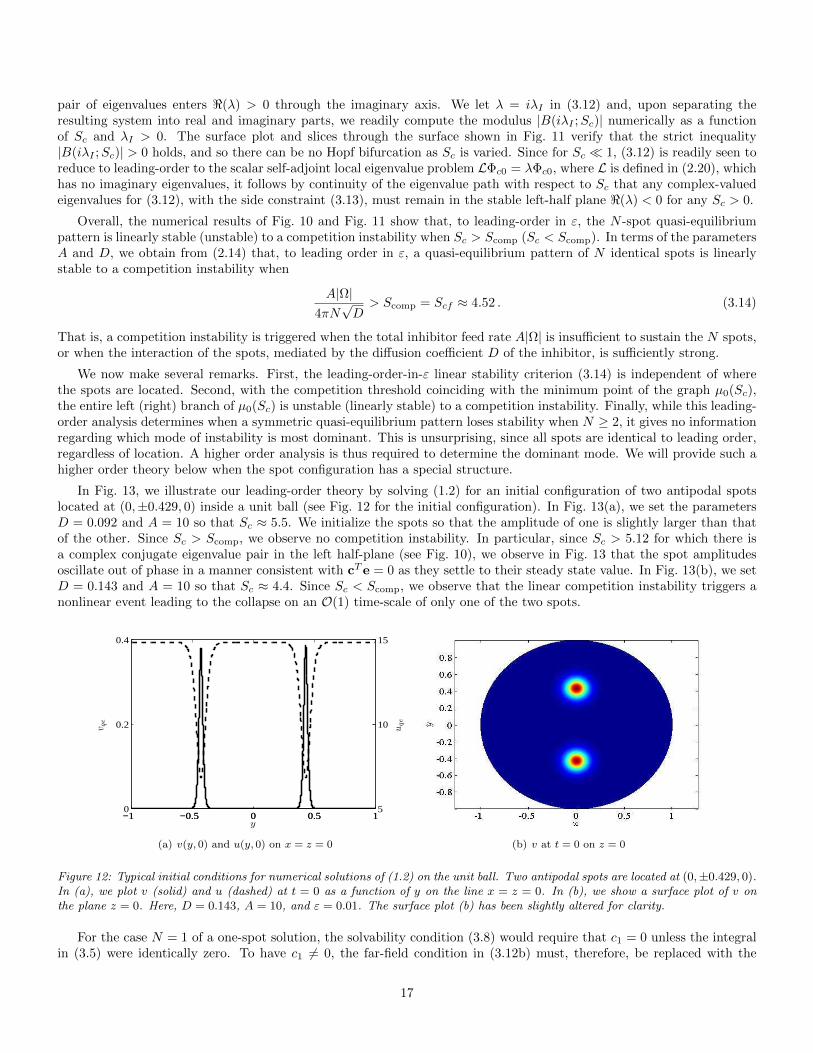
In Fig. 13, we illustrate our leading-order theory by solving (1.2) for an initial configuration of two antipodal spotslocated at (0,±0.429, 0) inside a unit ball (see Fig. 12 for the initial configuration). In Fig. 13(a), we set the parametersD = 0.092 and A = 10 so that Sc ≈ 5.5. We initialize the spots so that the amplitude of one is slightly larger than thatof the other. Since Sc > Scomp, we observe no competition instability. In particular, since Sc > 5.12 for which there isa complex conjugate eigenvalue pair in the left half-plane (see Fig. 10), we observe in Fig. 13 that the spot amplitudesoscillate out of phase in a manner consistent with cTe = 0 as they settle to their steady state value. In Fig. 13(b), we setD = 0.143 and A = 10 so that Sc ≈ 4.4. Since Sc < Scomp, we observe that the linear competition instability triggers anonlinear event leading to the collapse on an O(1) time-scale of only one of the two spots.

−1 −0.5 0 0.5 10

0.2

0.4

y

v qe

−1 −0.5 0 0.5 15

10

15

uqe

(a) v(y, 0) and u(y, 0) on x = z = 0 (b) v at t = 0 on z = 0

Figure 12: Typical initial conditions for numerical solutions of (1.2) on the unit ball. Two antipodal spots are located at (0,±0.429, 0).In (a), we plot v (solid) and u (dashed) at t = 0 as a function of y on the line x = z = 0. In (b), we show a surface plot of v onthe plane z = 0. Here, D = 0.143, A = 10, and ε = 0.01. The surface plot (b) has been slightly altered for clarity.

For the case N = 1 of a one-spot solution, the solvability condition (3.8) would require that c1 = 0 unless the integralin (3.5) were identically zero. To have c1 6= 0, the far-field condition in (3.12b) must, therefore, be replaced with the

17

0 2000 4000 6000 8000 10000

0.29

0.295

0.3

0.305

0.31

0.315

0.32

0.325

t

spot

amplitude

(a) Sc ≈ 5.5 > Scomp

0 10 20 30 40 50 600

0.1

0.2

0.3

0.4

0.5

t

spot

amplitude

(b) Sc ≈ 4.4 < Scomp

Figure 13: Plots of the amplitude of two antipodal spots located at (0,±0.429, 0) as computed from numerically solving (1.2) usingFlexPDE6 [6]. In (a), we set D = 0.092 and A = 10 so that Sc ≈ 5.5 > Scomp ≈ 4.52. The amplitudes appear to oscillate out ofphase as they settle to their steady state values. In (b), D = 0.143 and A = 10 so that Sc ≈ 4.4 < Scomp. The linear competitioninstability is seen to trigger a nonlinear event leading to the collapse of one of the two spots. In (a), ε = 0.02, while in (b), ε = 0.01.

condition that Ψ→ 1 as ρ→∞. That is, Ψ must be a constant at infinity. From a numerical solution of (3.12) with thismodified far-field behavior, we show in Fig. 14 that the eigenvalue with largest real part always lies in the left half-plane.Therefore, the one-spot solution is always linearly stable to a radially symmetric perturbation.

20 30 40 50 60 70 80−1

−0.8

−0.6

−0.4

−0.2

0

S

ℜ(λ)

(a) <(λ)

20 30 40 50 60 70 800

0.1

0.2

0.3

0.4

0.5

0.6

0.7

S

ℑ(λ)

(b) =(λ)

Figure 14: The real (a) and imaginary (b) parts of the eigenvalue with largest real part corresponding to a radially symmetricperturbation of a one-spot solution. The real part is negative for all S. For S . 10 (not shown), the largest eigenvalue becomes −1due to discretization, and is therefore absorbed into the continuous spectrum located on the negative real axis with λ ≤ −1.

Next, for N ≥ 2, we extend the leading-order stability theory to capture the weak effects on the stability thresholds ofthe locations of the spots for the special case where the spots are aligned so that e is an eigenvector of the Green’s matrixG. In the unit ball such patterns occur when spots are located at vertices of a platonic solid concentric within the ball,when spots are equally-spaced along an equator concentric within the ball, and for some of the equilibrium configurationsof the spot dynamics (4.13) derived below in §4. For such patterns, it follows from the fact that G is symmetric that itsmatrix spectrum is

Ge = k1e ; Gqj = kjqj , qTj e = 0 , j = 2, . . . , N , qTj qi = 0 , i 6= j . (3.15)

We recall from the discussion following (2.36) that when Ge = k1e, there is a common source-strength solution to

18

(2.34) that is the same as that for the leading-order solution in (2.14), i.e. that Sjε = Sc for all j = 1, . . . , N where Sc isdefined in (2.14). In addition, we have Ujε = Uc +O(ε2) and Vjε = Vc +O(ε2), so that B = B(λ;Sc)I +O(ε2) in (3.11).As a result, with a negligible error of O(ε2), we obtain for N ≥ 2 from (3.11) that

B(λ;Sc) = 4πεkj , when c = qj , j = 2, . . . , N . (3.16)

To determine the critical values for Sc at the stability threshold, we set λ = 0 in (3.16) and use B(0;Sc) = −µ′0(Sc),which yields the N − 1 nonlinear algebraic equations

µ′0(Sc) = −4πεkj , j = 2, . . . , N . (3.17)

To determine the root of (3.17) for each j, we expand Sc = Scf + εSj , and by using µ′0(Scf ) = 0, we readily calculate

Sj = − 4πkjµ′′0(Scf )

, j = 2, . . . , N . (3.18)

We conclude that there are zero-eigenvalue crossings whenever Sc = Scf + εSj + · · · for j = 2, . . . , N . The competition

instability threshold will then correspond to the largest of these possible values for Sj . Since µ′′0(Scf ) > 0 from Fig. 3(a),this threshold will be determined by the smallest of the eigenvalues of G in the subspace perpendicular to e. We summarizethis result as follows.

Main Result 3.1 Let ε→ 0 and N ≥ 2, and suppose that the spots are aligned so that e = (1, . . . , 1)T is an eigenvector ofthe Neumann Green’s matrix G. Then, the N -spot quasi-equilibrium solution is linearly stable to a competition instabilityon an O(1) time-scale if and only if

Sc > Scomp ≡ Scf −4πε

µ′′0(Sc)min

j=2,...,Nkj , where Sc ≡

A|Ω|4πN

√D. (3.19)

Here kj for j = 2, . . . , N are the eigenvalues of G in the subspace perpendicular to e (see (3.15)). In addition, Scf ≈ 4.52is the minimum point of the graph of µ0(Sc) versus Sc shown in Fig. 3(a), where we estimate that µ′′0(Scf ) ≈ 0.15.Equivalently, we predict that such a pattern is linearly stable on an O(1) time-scale if and only

D < Dcomp ≡(A|Ω|)2

16π2N2

(Scf −

4πε

µ′′0(Sc)min

j=2,...,Nkj

)−2

. (3.20)

For the unit ball, we now compare the prediction of (3.19) and (3.20) with full numerical results computed fromFlexPDE6 [6] for a symmetric two-spot pattern with spots at x1 = (0, 0, r0) and x2 = −x1, and for the four spottetrahedral pattern of Fig. 7(a) of §2.1. A pattern was classified as unstable when the amplitude of one of the spotscollapsed to zero on an O(1) time-scale (as in Fig. 13(b)) while deemed not to be caused by a triggering due to slow spotdynamics (see brief discussion below). Otherwise the pattern was classified as stable. The results of these computationsfor ε = 0.03, A = 10 are shown in Fig. 15(a) and Fig. 15(b), where numerically stable (unstable) parameter sets aremarked by solid (open) circles. The leading-order competition stability threshold is indicated by the dashed line, whilethe refined threshold is plotted in heavy solid. As expected, the smaller the distance between the spots, the smaller thediffusivity D must be in order for the pattern to be stable. We observe excellent agreement between the refined asymptotictheory and results from the full PDE solution.

Similarly, in Fig. 16(a) and Fig. 16(b) with ε = 0.03 and D = 1, we show a favorable comparison between the refinedstability threshold (3.19) and full numerical results computed from (1.2) using FlexPDE6 [6] for the case where N = 4spots are placed at the vertices of a tetrahedron of radius r0 < 1 concentric within the unit ball. The true steady-state ofthe slow dynamics is when r0 = 0.564 (see Table 1). For this case, there is a mode degeneracy in that k2 = k3 = k4, sothat up to O(ε) terms the entire 3-D subspace perpendicular to e goes unstable as Sc crosses below Scomp. As a result,although the refined stability theory determines the stability threshold, the linearized stability theory is not capable ofidentifying which mode of instability is dominant.

We make three remarks. First, with regards to numerically determining the stability of quasi-equilibrium patterns,the process was made difficult by the slow drift of concentric patterns to their equilibrium radius rc (see Table 1 of §4).When r0 > rc, an originally stable pattern may become unstable as the spots drift closer together. Starting close to

19

0.1 0.2 0.3 0.4 0.5 0.6 0.7 0.8 0.9r0

0.05

0.1

0.15

0.2

0.25

0.3

Dcomp

(a) Dcomp versus r0

0.1 0.2 0.3 0.4 0.5 0.6 0.7 0.8 0.9r0

3

3.5

4

4.5

5

5.5

6

Scomp

(b) Scomp versus r0

Figure 15: Comparison of the predictions of the refined competition stability threshold (3.19) (solid curves) with the full numericalresults computed from (1.2) using FlexPDE6 [6] for a two-spot pattern with spots at x1 = (0, 0, r0) and x2 = −x1 for A = 10 andε = 0.03 inside the unit ball. The vertical axis is D (left panel) and S (right panel). The solid (open) dots represent parameter setswhere the pattern was observed numerically from FlexPDE6 to be stable (unstable). The horizontal dotted lines are the leading-order

competition thresholds Dcomp ≡(A2S−2

cf

)/36 ≈ 0.136 (left panel) and Scomp ≡ Scf ≈ 4.52 (right panel).

0.1 0.2 0.3 0.4 0.5 0.6 0.7 0.8 0.9r0

40

45

50

55

60

65

70

Acomp

(a) Acomp versus r0

0.1 0.2 0.3 0.4 0.5 0.6 0.7 0.8 0.9r0

3

3.5

4

4.5

5

5.5

6

Scomp

(b) Scomp versus r0

Figure 16: Comparison of the predictions of the refined competition stability threshold (3.19) (solid curves) with the full numericalresults computed from (1.2) using FlexPDE6 [6] for a four-spot pattern with spots centered at the vertices of a tetrahedron ofradius r0 < 1 concentric within the unit ball. The parameters are D = 1 and ε = 0.03. The vertical axis is the competitioninstability threshold for A (left panel) and S (right panel). The solid (open) dots represent parameter sets where the pattern wasobserved numerically from FlexPDE6 to be stable (unstable). The horizontal dotted lines are the leading-order competition thresholdsAcomp ≡ 12

√DScf ≈ 54.24 (left panel) and Scomp = Scf ≈ 4.52 (right panel).

20

threshold, the dynamics can destabilize a pattern rather quickly when ε is only moderately small. A pattern thus neededto be initialized farther below threshold in order to be more assuredly classified as stable, resulting in apparently pooreragreement with asymptotics when r0 > rc. When r0 < rc, dynamics increase distances between spots so that an originallystable pattern will remain stable for all time. On the other hand, the O(1) instability of an unstable pattern will triggerbefore the O(ε3) dynamics can stabilize it. This results in seemingly better agreement with asymptotics when r0 < rc.Second, even though the linear theory predicts that all modes destabilize simultaneously at S = Scomp, we have onlynumerically observed the annihilation of a single spot at a time, regardless of initial conditions. This mode selection maybe due to an effect of higher order than the above analysis can capture. Finally, for the case where e is not an eigenvectorof G, it is much more challenging to calculate ε-dependent correction terms to the leading-order competition stabilitythreshold Scf , and we do not perform this analysis here. This difficulty arises due to the need to resolve the intricateimperfection-sensitive bifurcation structure that exists near Scf whenever e is not an eigenvector of G.

3.1 Linear Stability of Asymmetric Patterns

In this subsection we briefly formulate the leading-order linear stability problem for the asymmetric patterns of (2.21).It is beyond the scope of this paper to give a comprehensive study of the stability of these patterns, and we only givea partial result showing the instability of asymmetric patterns for which Nr ≥ N`. While previous studies of 2-D spotproblems (cf. [25], [18]) have found that certain asymmetric patterns can be stable in a particular regime, we have notbeen able to numerically observe any stable asymmetric patterns (even when Nr < N`) in the 3-D Schnakenberg model,perhaps owing to the small domain of attraction of such patterns.

The formulation of the linear stability problem proceeds in a similar manner as for the symmetric pattern, with thecritical difference being that B(λ;S) need not be zero. The relationship B(λ;S) must therefore be determined in order

to determine stability. To begin, we index the spots so that spots corresponding to strength S`,r are located at x(`,r)j , for

j = 1, . . . , N`,r. Then, in the inner region near x(`,r)j where (vqe, uqe) ∼ (

√Dν(`,r), µ(`,r)/

√D), we let φ ∼ c

(`,r)j Φ(`,r)(ρ)

and ψ ∼ c(`,r)j Ψ(`,r)(ρ)/D in (3.2). This results in the inner eigenvalue problem of (3.4) with the far-field condition

Ψ(`,r) ∼ 1/ρ+B(λ;S`,r). By the same matching procedure leading to (3.10), we have that

c(`)j B(λ;S`)

D= ψ0 ,

c(r)j B(λ;Sr)

D= ψ0 . (3.21)

The weights associated with the perturbation of each type of spot must then have a common value, so that

c(`)j = c` , j = 1, . . . , N` ; c

(r)j = cr , j = 1, . . . , Nr . (3.22)

Together with (3.21), (3.22) yields one equation for c` and cr,

B(λ;S`)c` −B(λ;Sr)cr = 0 , (3.23a)

while the second equation comes from the solvability condition (3.8), which we rewrite as

N`c` +Nrcr = 0 . (3.23b)

A nontrivial solution to the system (3.23) exists if and only if λ satisfies the transcendental equation K(λ) = 0, where

K(λ) ≡ NrN`

+B(λ;Sr)

B(λ;S`), (3.24)

where for given positive integers Nr and N`, the source strengths S` and Sr are determined by the nonlinear algebraicsystem (2.22). The asymmetric pattern is unstable if (3.24) has a root in <(λ) > 0, and is linearly stable if all roots to(3.24) are in <(λ) < 0.

We now give a numerically-assisted proof for the existence of at least one positive real root of (3.24) when Nr ≥ N`.We first recall that B(0, S) = −µ′0(S). Together with the one-sided inverse functions S` = S`(µ0) and Sr = Sr(µ0) of themap µ0(S), we obtain

21

K(0) ≡ NrN`−D(µ0) ; D(µ0) ≡ −µ

′0 [Sr(µ0)]

µ′0 [S`(µ0)]> 0 . (3.25)

The function µ0(S) is shown in Fig. 3(a). Observe that µ′0(S) > 0 (µ′0(S) < 0) when S > Scf (S < Scf ). In Fig. 17(a)we plot the numerically computed function D(µ0) versus µ0 on µ0 > µ0min, where µ0min = µ0(Scf ). By L’Hopital’s rulewe must have D(µ0min) = 1. However, our plot in Fig. 17(a) shows that 0 < D(µ0) < 1 for µ0 > µ0min. Therefore,when Nr ≥ N`, we have from (3.25) that K(0) > 0. Next, we note that because the entire right branch of µ0(S)is stable with respect to positive real eigenvalues, B(λ;Sr) must be of only one sign when λ is positive real. WithB(0;Sr) = −µ′0[Sr(µ0)] < 0, we have that B(λ;Sr) < 0 for all λ > 0. Now since the left branch is unstable to acompetition instability, there must exist a λc positive real such that B(λc;S`) = 0. With B(0;S`) = −µ′0[S`(µ0)] > 0, wemust have B(λ;S`) > 0 when 0 < λ < λc. Therefore, as λ→ λ−c , K → −∞. Using that K(0) > 0 whenever Nr ≥ N`, weconclude from the intermediate value theorem that there must exist a positive real root 0 < λr < λc to (3.24). As such,all asymmetric patterns of (2.21) with Nr ≥ N` are unstable to a monotonic instability. In Fig. 17(b), we show typicalcurves for B(λ;S`) (dashed) and B(λ;Sr) (solid) for λ > 0 with S` = 3.06 and Sr = 6.99. Here, B(λ;S`) crosses 0 atλc ≈ 0.65 while B(λ;Sr) is of constant sign. In Fig. 17(c), we plot the positive real root satisfying 0 < λr < λc of K(λ)in the case N` = Nr = 1. As A|Ω|/(4π(2)

√D)→ S+

cf , the asymmetric pattern approaches a symmetric two-spot patternwith S1 = S2 = Scf . From the leading-order stability theory, this pattern is neutrally stable with a zero eigenvalue,consistent with Fig. 17(c).

The argument above cannot in general be applied when Nr < N`. Numerical solutions of K(λ) = 0 in the case Nr = 1and N` = 3 (dotted branch in the right panel of Fig. 5) indicate that the solution at the saddle node is neutrally stable,while the upper branch is unstable to a real positive eigenvalue. There is no positive real root of K(λ) on the lower branch,though numerical solutions of the full PDE still indicate that these solutions are monotonically unstable. This may bedue to a small domain of attraction of solutions on the lower branch. A full characterization of the stability of asymmetricbranches with Nr < N`, as well as a refined stability theory for general asymmetric patterns, is beyond the scope of thispaper.

5 10 150

0.2

0.4

0.6

0.8

1

µ0

−µ′ 0(S

r)/µ′ 0(S

ℓ)

(a) D versus µ0

0 2 4 6 8 10λ

-2

-1.5

-1

-0.5

0

0.5

B(λ;3.06),B(λ,6.99)

(b) B(λ; 3.06), B(λ; 6.99)

4.5 5 5.5 6 6.5 7 7.5 8A|Ω|/(4π(2)

√D)

0

0.2

0.4

0.6

0.8

1

1.2λr

(c) λr for N` = Nr = 1

Figure 17: In (a), we plot D(µ0) defined in (3.25) versus µ0 on µ0 > µ0min. Here, S` < Scf (Sr > Scf ) is the smaller (larger)value of S associated with µ0(S) (see Fig. 3(a)). In (b), we plot B(λ;S`) (dashed) and B(λ;S`). Here, S` = 3.06 and Sr = 6.99are solutions of (2.22) with N` = Nr = 1 and A|Ω|/(4π

√D) = 10.05. For the particular parameters used, B(λ;S`) crosses 0

at λc ≈ 0.65 while B(λ;Sr) has constant sign. In (c), with N` = Nr = 1, we plot the positive root of K(λ) in (3.24) satisfying0 < λr < λc. Observe that λr → 0+ as A|Ω|/(4π(2)

√D)→ S+

cf .

3.2 Spot Self-Replication: A Peanut-Splitting Instability

Next, we analyze the linear stability of a quasi-equilibrium pattern to localized radially asymmetric perturbations neareach spot. Because this instability to leading order is local and does not involve coupling between spots, the same analysisapplies to both symmetric and asymmetric patterns. In the j-th inner region, we use the local behavior (2.17) andφ(xj + εy) = Φ(y) and ψ(xj + εy) = Ψ(y)/D to write (3.2) as

22

10 20 30 40 50 60−1

−0.5

0

0.5

1

S

λ

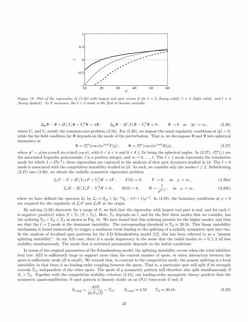
Figure 18: Plot of the eigenvalue of (3.28) with largest real part versus S for ` = 2 (heavy solid), ` = 3 (light solid), and ` = 4(heavy dashed). As S increases, the ` = 2 mode is the first to become unstable.

∆yΦ− Φ + 2UcVcΦ + V 2c Ψ = λΦ , ∆yΨ− 2UcVcΦ− V 2

c Ψ = 0 , Φ→ 0 as |y| → ∞ , (3.26)

where Uc and Vc satisfy the common core problem (2.16). For (3.26), we impose the usual regularity conditions at |y| = 0,while the far-field condition for Ψ depends on the mode of the perturbation. That is, we decompose Φ and Ψ into sphericalharmonics as

Φ = Pm` (cosφ)eimθF (ρ) , Ψ = Pm` (cosφ)eimθH(ρ) , (3.27)

where yt = ρ(sinφ cos θ, sinφ sin θ, cosφ), with 0 < φ < π and 0 < θ ≤ 2π being the spherical angles. In (3.27), Pm` (z) arethe associated Legendre polynomials, ` is a positive integer, and m = 0, . . . , `. The ` = 1 mode represents the translationmode for which λ = O(ε3); these eigenvalues are captured in the analysis of slow spot dynamics studied in §4. The ` = 0mode is associated with the competition instability studied in §3. As such, we consider only the modes ` ≥ 2. Substituting(3.27) into (3.26), we obtain the radially symmetric eigenvalue problem

L`F − F + 2UcVcνF + V 2c H = λF , F (0) = 0 , F → 0 , as ρ→∞ , (3.28a)

L`H − 2UcVcF − V 2c H = 0 , H(0) = 0 , H ∼ 1

ρ`+1, as ρ→∞ , (3.28b)

where we have defined the operator L` by L` ≡ ∂ρρ + 2ρ−1∂ρ − `(`+ 1)ρ−2. In (3.28), the boundary conditions at ρ = 0are required for the regularity of L`F and L`H at the origin.

By solving (3.28) discretely for a range of S, we find that the eigenvalue with largest real part is real, and for each `,is negative (positive) when S < Σ` (S > Σ`). Here, Σ` depends on `, and for the first three modes that we consider, hasthe ordering Σ2 < Σ3 < Σ4 as shown in Fig. 18. We have found that this ordering persists for the higher modes, and thussee that the ` = 2 mode is the dominant instability. The corresponding threshold is Σ2 ≈ 20.16. This linear instabilitymechanism is found numerically to trigger a nonlinear event leading to the splitting of a radially symmetric spot into two.In the analysis of localized spot patterns for the 2-D Schnakenberg model [12], this has been referred to as a “peanutsplitting instability”. In our 3-D case, there is a mode degeneracy in the sense that the radial modes m = 0, 1, 2 all losestability simultaneously. The mode that is activated presumably depends on the initial conditions.

In terms of the original parameters of the Schnakenberg model, the splitting instability occurs when the total inhibitorfeed rate A|Ω| is sufficiently large to support more than the current number of spots, or when interaction between thespots is sufficiently weak (D is small). We remark that, in contrast to the competition mode, the peanut splitting is a localinstability in that there is no leading-order coupling between the spots. That is, a particular spot will split if its strengthexceeds Σ2, independent of the other spots. The spots of a symmetric pattern will therefore also split simultaneously ifSc > Σ2. Together with the competition stability criterion (3.14), our leading-order asymptotic theory predicts that thesymmetric quasi-equilibrium N -spot pattern is linearly stable on an O(1) time-scale if only if

Scomp <A|Ω|

4πN√D< Σ2 ; Scomp ≈ 4.52 Σ2 ≈ 20.16 . (3.29)

23

These thresholds are equivalent to thresholds for A given in (1.3), and are in excellent agreement with numerics asfigures 1 and 2 show.

Figure 19: Numerical simulation of (1.2a) showing self-replication process of seven spots. Here, ε = 0.06 and A is very slowlyincreased according to the formula A = 200+ε4t. Snapshots show the value of A at the self-replication thresholds. Next to the spots,the value of (Ge)j is also given. Asymptotics predict that the spot with the smallest value of (Ge)j will be the one that self-replicates.

The leading-order thresholds (1.3) provide an excellent prediction for when the splitting first starts to occur, but doesnot predict which spot(s) will split. In fact, it is surprising that only one spot splits at a time. Indeed, on snapshot#7 of Figure 1 (A = 173.248), one can observe at least two spots initiate the deformation (right and center spots).However, eventually only the center spot undergoes splitting. This is also very different qualitatively from either one ortwo dimensions. For example in [12], the authors performed an analogous experiment in two dimensions, and observedincreasing A past the threshold resulted in multiple spots splitting simultaneously. Similarly, in one dimension, multiplespots tend to replicate simultaneously [11]. A two-order expansion of Sj – see (2.35) – shows that the largest Sj correspondsto the smallest value of (Ge)j . This suggests that as A is increased, the spot that self-replicates is the one with the smallestvalue of (Ge)j . Figure 19 shows self-replication with 7 spots. The value of (Ge)j is indicated for each spot in the figure.While all of these values are rather close, the self-replicating spot is indeed the one with the smallest such value (-0.27).

4 Slow Spot Dynamics

In this section, we analyze the slow dynamics associated with an N -spot quasi-equilibrium solution. To derive an ODEsystem characterizing the slow spot dynamics, we must extend the calculation in §2 to one higher order. We will proceedby the method summarized at the end of §2.1. In the inner region near the j-th spot, we let xj = xj(σ) where σ = ε3t,and expand the inner solution as

y = ε−1(x−xj(σ)) , v(xj+εy) =√D[Vjε(ρ) + ε2Vj2(y) + · · ·

], u(xj+εy) =

1√D

[Ujε(ρ) + ε2Uj2(y) + · · ·

], (4.1)

with ρ ≡ |y|, where Ujε, Vjε satisfy the radially symmetric core problem

∆ρVjε − Vjε + UjεV2jε = 0 , V ′jε(0) = 0 , Vjε → 0 , as ρ→∞ , (4.2a)

∆ρUjε − UjεV 2jε = 0 , U ′jε(0) = 0 , (4.2b)

with far-field behaviorUjε ∼ µj − Sjε/ρ+ · · · , as ρ→∞ , (4.2c)

where µj ≡ µ0(Sjε). The corresponding outer solution (see (2.33)) is given by

u ∼ ξ − 4πε√D

N∑

i=1

SiεG(x; xi) ,

N∑

i=1

Siε =A|Ω|

4π√D, (4.3)

24

where Sjε, for j = 1, . . . , N , and ξ satisfy the nonlinear algebraic system (2.34).

We first expand u as x → xj , while retaining the higher-order gradient terms associated with the Green’s function.Upon using (2.10b), we obtain in terms of inner variables that

u ∼ ξ − Sjε√Dρ− 4πε√

D(GS)j −

4πε2

√D

y·

Sjε∇xR(x; xj)|x=xj +

N∑

i=1

i 6=j

Siε∇xG(x; xi)|x=xj

, as x→ xj , (4.4)

where G is the Neumann Green’s matrix. The O(ε2) term in (4.4) is the motivation for the form of the higher-orderexpansion in (4.1) and the scaling for the slow time-scale σ = ε3t.

Upon substituting (4.1) into (1.2), and matching the inner solution to the O(ε2) term in (4.4), we obtain thatW2 = (Vj2, Uj2)T satisfies

LW2 ≡ ∆yW2 +MεW2 = −(

x′j ·∇yVjε0

), y ∈ R2 ; W2 ∼

(0

bj · y

), as |y| → ∞ . (4.5a)

Here the 2× 2 matrix Mε and the vector bj are defined by

Mε ≡( −1 + 2UjεVjε V 2

jε−2UjεVjε −V 2

jε

), bj ≡ −4πSjε∇xR(x; xj)|x=xj − 4π

N∑

i=1

i 6=j

Siε∇xG(x; xi)|x=xj . (4.5b)

Let y = (y1, y2, y3)T and Wjε ≡ (Vjε, Ujε)T . We observe upon differentiating the core problem (4.2) with respect toi-th coordinate yi of y that

L (∂yiWjε) = 0 where ∂yiWjε ≡ ρ−1

(V ′jε(ρ)U ′jε(ρ)

)yi , for i = 1, 2, 3 .

This shows that the dimension of the nullspace of L, and consequently L?, is at least three-dimensional. We will assumethat this nullspace is exactly three-dimensional, which we can verify numerically provided that Sjε does not coincide withthe critical value Σ2 ≈ 20.16 for the peanut-splitting instability.

From a Fredholm alternative criterion, the following lemma provides a necessary condition for (4.5) to have a solution.

Lemma 4.1 A necessary condition for (4.5) to have a solution is that xj(σ) satisfies

x′j = − 3

κ1bj , κ1 = κ1(Sjε) ≡

∫ ∞

0

ρ2P1(ρ)V ′jε(ρ) dρ , (4.6)

where P1(ρ) is the first component of P(ρ) ≡ (P1(ρ), P2(ρ))T , which satisfies

∆ρP−2

ρ2P +MT

εP = 0 , 0 < ρ <∞ ; P ∼(

01/ρ2

), as ρ→∞ , (4.7)

and P = O(ρ) as ρ→ 0, where ∆ρP ≡ P′′ + 2ρ−1P′.

Proof: We first seek three independent nontrivial solutions to the homogeneous adjoint problem L?Ψ ≡ ∆yΨ+MTεΨ = 0

in the form Ψi ≡ P(ρ)yi/ρ for i = 1, . . . , 3. Since

∆y [Pyi/ρ] =

(∆ρP−

2

ρ2P

)yiρ,

we readily obtain that P(ρ) satisfies ∆ρP− 2ρ−2P +MTεP = 0. To establish the far-field behavior of P, we obtain using

(4.5b) forMε, and the fact that Vj0 → 0 exponentially as ρ→∞, that P2(ρ) satisfies P ′′2 +2ρ−1P ′2−2ρ−2P2 ≈ 0 for ρ 1.The decaying solution to this Euler’s equation implies that P2 = O(ρ−2) as ρ→∞, and the eigenfunction is normalized

25

by imposing the precise behavior that P2 ∼ 1/ρ2 as ρ→∞. In contrast, for P1(ρ) we obtain that P ′′1 + 2ρ−1P ′1 − P1 ≈ 0as ρ→∞, so that P1 decays exponentially as ρ→∞. In this way, we obtain that P satisfies (4.7).

Next, to derive our solvability condition we use Green’s identity over a large ball of radius |y| = ρ0 1 to obtain that

limρ0→∞

∫

Ωρ0

(ΨTi LW2 −WT

2 L?Ψi

)dy = lim

ρ0→∞

∫

∂Ωρ0

(ΨTi ∂ρW2 −WT

2 ∂ρΨi

) ∣∣∣ρ=ρ0

dS . (4.8)

With Ψi ≡ P(ρ)yi/ρ, and for a fixed i ∈ 1, 2, 3, we first calculate the left-hand side of this expression using (4.5a) toobtain

limρ0→∞

∫

Ωρ0

(ΨTi LW2 −WT

2 L?Ψi

)dy = − lim

ρ0→∞

∫

Ωρ0

yiρP1(ρ)

(x′j ·∇yVjε

)dy ,

= −3∑

k=1

x′jk limρ0→∞

∫

Ωρ0

yiykρ2

V ′jε(ρ)P1(ρ) dy , (4.9)

where x′j ≡ (x′j1, x′j2, x

′j3)T . By using symmetry considerations, we readily establish that

∫Ωρ0

yiykf(ρ) dy = 0 when i 6= k

and∫

Ωρ0y2i f(ρ) dy = 4π

3

∫ ρ00ρ4f(ρ) dρ for any radially symmetric function f(ρ). In this way, the last expression (4.9)

becomes

limρ0→∞

∫

Ωρ0

(ΨTi LW2 −WT

2 L?Ψi

)dy = −4π

3x′ji

∫ ∞

0

ρ2P1(ρ)V ′jε(ρ) dρ . (4.10)

Next, we calculate the right-hand side of (4.8). For the first term on the right-hand side of (4.8) we use P2(ρ) ∼ 1/ρ2,Uj1 ∼ bj ·y and ∂ρUj1 ∼ bj ·y/ρ as ρ→∞, to estimate that

limρ0→∞

∫

∂Ωρ0

ΨTi ∂ρW2|ρ=ρ0 dS = lim

ρ0→∞

∫

∂Ωρ0

P2(ρ)yiρ∂ρUj1

∣∣∣ρ=ρ0

dS = limρ0→∞

∫

∂Ωρ0

yiρ4

(bj ·y)∣∣∣ρ=ρ0

dS .

Then, since∫∂Ωρ0

yiykf(ρ)|ρ=ρ0 dS = 0 for i 6= k, and writing dS = ρ20dΩ0, where dΩ0 is the solid angle for the unit ball,

we obtain that

limρ0→∞

∫

∂Ωρ0

ΨTi ∂ρW2|ρ=ρ0 dS = lim

ρ0→∞

∫

∂Ωρ0

y2i

ρ20

bji dΩ0 =4π

3bji , (4.11)

for each i = 1, 2, 3. In a similar way, we can calculate the second boundary integral in (4.8) as

− limρ0→∞

∫

∂Ωρ0

WT2 ∂ρΨi|ρ=ρ0 dS = − lim

ρ0→∞

∫

∂Ωρ0

(bj ·y) ∂ρ

[P2(ρ)

yiρ

] ∣∣∣ρ=ρ0

ρ20 dΩ0 ,

= − limρ0→∞

∫

∂Ωρ0

(bj ·y) ∂ρ

(yiρ3

) ∣∣∣ρ=ρ0

ρ20 dΩ0 ,

= limρ0→∞

∫

∂Ωρ0

(bj ·y)

(2yiρ4

) ∣∣∣ρ=ρ0

ρ20 dΩ0 ,

= 2 limρ0→∞

∫

∂Ωρ0

bjiy2i

ρ20

∣∣∣ρ=ρ0

dΩ0 =8π

3bji . (4.12)

By adding (4.11) and (4.12), we obtain that the right-hand side of (4.8) is 4πbji. Finally, by equating this expression withthat given in (4.10) for the left-hand side of (4.8), we obtain that x′ji = −3bji/κ1, where κ1 is defined in (4.6). In vectorform, with i = 1, 2, 3, we obtain (4.6).

By combining (4.6) with our expression for bj in (4.5b), we obtain an ODE-DAE system for the slow spot dynamicsgiven by

dxjdt

=12πε3

κ1

Sjε∇xR(x; xj)|x=xj +

N∑

i=1

i 6=j

Siε∇xG(x; xi)|x=xj

, j = 1, . . . , N , (4.13)

26

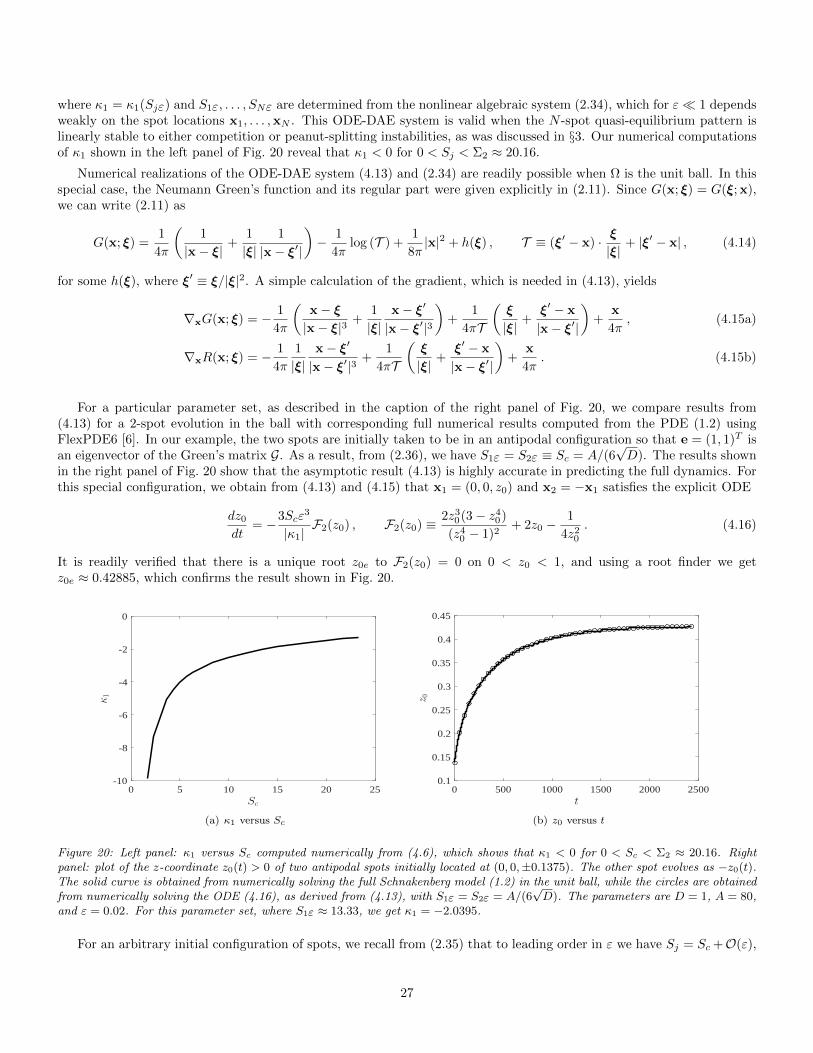
where κ1 = κ1(Sjε) and S1ε, . . . , SNε are determined from the nonlinear algebraic system (2.34), which for ε 1 dependsweakly on the spot locations x1, . . . ,xN . This ODE-DAE system is valid when the N -spot quasi-equilibrium pattern islinearly stable to either competition or peanut-splitting instabilities, as was discussed in §3. Our numerical computationsof κ1 shown in the left panel of Fig. 20 reveal that κ1 < 0 for 0 < Sj < Σ2 ≈ 20.16.

Numerical realizations of the ODE-DAE system (4.13) and (2.34) are readily possible when Ω is the unit ball. In thisspecial case, the Neumann Green’s function and its regular part were given explicitly in (2.11). Since G(x; ξ) = G(ξ; x),we can write (2.11) as

G(x; ξ) =1

4π

(1

|x− ξ| +1

|ξ|1

|x− ξ′|

)− 1

4πlog (T ) +

1

8π|x|2 + h(ξ) , T ≡ (ξ′ − x) · ξ

|ξ| + |ξ′ − x| , (4.14)

for some h(ξ), where ξ′ ≡ ξ/|ξ|2. A simple calculation of the gradient, which is needed in (4.13), yields

∇xG(x; ξ) = − 1

4π

(x− ξ

|x− ξ|3 +1

|ξ|x− ξ′

|x− ξ′|3)

+1

4πT

(ξ

|ξ| +ξ′ − x

|x− ξ′|

)+

x

4π, (4.15a)

∇xR(x; ξ) = − 1

4π

1

|ξ|x− ξ′

|x− ξ′|3 +1

4πT

(ξ

|ξ| +ξ′ − x

|x− ξ′|

)+

x

4π. (4.15b)

For a particular parameter set, as described in the caption of the right panel of Fig. 20, we compare results from(4.13) for a 2-spot evolution in the ball with corresponding full numerical results computed from the PDE (1.2) usingFlexPDE6 [6]. In our example, the two spots are initially taken to be in an antipodal configuration so that e = (1, 1)T isan eigenvector of the Green’s matrix G. As a result, from (2.36), we have S1ε = S2ε ≡ Sc = A/(6

√D). The results shown

in the right panel of Fig. 20 show that the asymptotic result (4.13) is highly accurate in predicting the full dynamics. Forthis special configuration, we obtain from (4.13) and (4.15) that x1 = (0, 0, z0) and x2 = −x1 satisfies the explicit ODE

dz0

dt= −3Scε

3

|κ1|F2(z0) , F2(z0) ≡ 2z3

0(3− z40)

(z40 − 1)2

+ 2z0 −1

4z20

. (4.16)

It is readily verified that there is a unique root z0e to F2(z0) = 0 on 0 < z0 < 1, and using a root finder we getz0e ≈ 0.42885, which confirms the result shown in Fig. 20.

0 5 10 15 20 25Sc

-10

-8

-6

-4

-2

0

κ1

(a) κ1 versus Sc

0 500 1000 1500 2000 2500t

0.1

0.15

0.2

0.25

0.3

0.35

0.4

0.45

z0

(b) z0 versus t

Figure 20: Left panel: κ1 versus Sc computed numerically from (4.6), which shows that κ1 < 0 for 0 < Sc < Σ2 ≈ 20.16. Rightpanel: plot of the z-coordinate z0(t) > 0 of two antipodal spots initially located at (0, 0,±0.1375). The other spot evolves as −z0(t).The solid curve is obtained from numerically solving the full Schnakenberg model (1.2) in the unit ball, while the circles are obtainedfrom numerically solving the ODE (4.16), as derived from (4.13), with S1ε = S2ε = A/(6

√D). The parameters are D = 1, A = 80,

and ε = 0.02. For this parameter set, where S1ε ≈ 13.33, we get κ1 = −2.0395.

For an arbitrary initial configuration of spots, we recall from (2.35) that to leading order in ε we have Sj = Sc +O(ε),

27

where Sc is given in (2.14). Then, upon introducing the discrete energy H(x1, . . . ,xN ) defined by

H(x1, . . . ,xN ) ≡N∑

i=1

R(xi; xi) + 2

N∑

i=1

N∑

j>i

G(xi; xj) , (4.17)

we can write (4.13) in the form of a gradient flow. The result is summarized as follows:

Main Result 4.2 Let ε → 0, and suppose that the N -spot quasi-equilibrium solution of (1.2) is linearly stable on anO(1) time-scale to either competition or peanut-splitting instabilities. Then, to leading order in ε, the collection of spotsevolve by the gradient flow

dxjdt

= −6πε3Sc|κ1|

∇xjH(x1, . . . ,xN ) , j = 1, . . . , N ; Sc =A|Ω|

4πN√D, (4.18)

where the discrete energy H is defined in (4.17). Here κ1 = κ1(Sc) is defined in (4.6). In terms of the spatial configurationx1, . . . ,xN of spots, a two-term expansion for the spot strengths when µ′0(Sc) 6= 0 is

Sjε ∼ Sc +4πεScµ′0(Sc)

(eTGe

N− (Ge)j

)+ · · · , j = 1, . . . , N , (4.19)

where e = (1, . . . , 1)T and G is the Neumann Green’s matrix.

We now use (4.18) to discuss possible steady-state spot configurations. It follows from (4.18) that spatial configurationsof steady-state spots are critical points of the discrete energy H, and that patterns that are linearly stable with respectto the ODE dynamics (4.18) are minima of H. The discrete energy H also arises in the analysis of the mean first passagetime for a Brownian walk in a 3-D domain with small localized spherical traps (cf. [3]). Following the decomposition in[3], we define H0 by

H(x1, . . . ,xN ) =H0

4π− 7N2

10π, H0 ≡ 4π

N∑

i=1

(R(xi; xi) +

7

10π

)+ 2

N∑

i=1

N∑

j>i

(G(xi; xj) +

7

10π

) . (4.20)

For the unit ball, in Table 1 we give some results for N = 2, . . . , 20 computed in [3] using numerical optimization softwarefor a restricted optimization problem whereby H0 is minimized subject to the condition that either all N spots must be ona single ring (second and third columns), or all N − 1 points are on a single ring while the remaining spot is at the origin(fourth and fifth columns). From this table we observe for N ≥ 16 that the second class of patterns gives a smaller H0.It was found in [3] that, for N = 2, . . . , 20, an unrestricted optimization of H0 gives results that coincide to the numberof digits shown with the restricted minimum energies in Table 1, with all spots being very close to, but not exactly on, acommon ring of radius rc. As a result, for N = 2, . . . , 20, the global minimum of H0 can be predicted rather accuratelyfrom the restricted optimization results in Table 1.

Point configurations corresponding to such global minima of H0 are linearly stable equilibria of the ODE dynamics(4.18). We then perform numerical simulations of (4.18) with randomly generated initial conditions in an attempt toclassify steady-states of (4.18) with large basins of attraction of initial conditions. We find for N = 2, 3, 4, 6, 8 that thecomputed steady-state solutions agree precisely with those for the one-ring patterns shown in the second and third columnsin Table 1 and that, for these values of N , e = (1, . . . , 1)T is an eigenvector of the Green’s matrix G at the steady-state. Inparticular, for N = 2, the first row of Table 1 predicts that a two-spot steady-state of (4.18) will correspond to antipodalspots on an interior ball of radius rc ≈ 0.429, which is precisely what was observed in the results shown in the right panelof Fig. 20. In addition, for N = 4, we observe from Table 1 that the bifurcation diagram shown in Fig. 7(a) correspond totrue steady-state solutions. Moreover, our numerical results show for N = 12 that some initial conditions lead for (4.18)lead to a steady-state where the spots are centered at the vertices of an icosahedron with discrete energy and radius givenin Table 1, for which e is an eigenvector of G, while other initial conditions lead to a pattern with 11 spots nearly on acommon ring with a spot at the center. For N = 13, 14, 15, initial conditions lead either to spots nearly on a common ringor to the near-ring and center-hole pattern. For N = 16, . . . , 20 our computations of (4.18) lead typically to the near-ringand center-hole pattern. For N = 12, . . . , 20, we find that the discrete energies at the steady-state coincide very closelywith the restricted optimization results in Table 1. For N = 5, our simulations of (4.18) with random initial conditions,shows that (4.18) converges to a steady-state with 2 antipodal spots at a distance of 0.59279 from the origin, and with 3spots equally-spaced on a mid-plane with spots being at a distance 0.59605 from the origin.

28

N H(a)0 Spherical radii H(b)

0 Spherical radii

rj = rc ∀j rj = rc ∀j , (r1 = 0)

2 7.2763 0.429 9.0316 0.563

3 18.5047 0.516 20.3664 0.601

4 34.5635 0.564 36.8817 0.626

5 56.2187 0.595 58.1823 0.645

6 82.6490 0.618 85.0825 0.659

7 115.016 0.639 116.718 0.671

8 152.349 0.648 154.311 0.680

9 195.131 0.659 196.843 0.688

10 243.373 0.668 244.824 0.694

11 297.282 0.676 297.283 0.700

12 355.920 0.683 357.371 0.705

13 420.950 0.689 421.186 0.710

14 491.011 0.694 491.415 0.713

15 566.649 0.698 566.664 0.717

16 647.738 0.702 647.489 0.720

17 734.344 0.706 733.765 0.722

18 826.459 0.709 825.556 0.725

19 924.360 0.712 922.855 0.727

20 1027.379 0.715 1025.94 0.729

Table 1: Numerically computed minimal values of the discrete energy function H0 for the optimal arrangement of N-traps withina unit ball where the optimization is restricted to a one-ring configuration H(a)

0 , or to a one-ring configuration with a center spot

H(b)0 (see [3]). The minimum of these two values is shown in bold face. The unrestricted optimization of H0 gives results extremely

close to the restricted minimum energies in Table 1, but that not all spots lie exactly on a ring of a common radius.

29

4.1 Spot Dynamics with a Spatially Varying Feed-Rate

In this subsection we extend our previous analysis of (1.2) to the case where the feed-rate A depends on x, with A(x) > 0in Ω. We only briefly highlight the new features of the analysis needed when A = A(x).

We proceed by the method discussed at the end of §2.1. Since the inner solution near each spot does not depend onA, we can proceed as in §2.1 to allow the source strength Sj in (2.2) to depend weakly on ε, and so we write Ujε, Vjε tobe the solution to (2.2) for which Ujε ∼ µj − Sjε/ρ as ρ→∞, where µj ≡ µ0(Sjε). In place of (2.32), the outer solutionnow satisfies

∆u ∼ −εA(x)

D+

4πε√D

N∑

j=1

Sjεδ(x− xj) , x ∈ Ω ; ∂nu = 0 , x ∈ ∂Ω . (4.21)

By the divergence theorem, we obtain that

N∑

i=1

Siε =A|Ω|

4π√D, A ≡ 1

|Ω|

∫

Ω

A(x) dx . (4.22)

The exact solution to (4.21) is simply

u = ξ +ε

Du1p(x)− 4πε√

D

N∑

i=1

SiεG(x; xi) , (4.23)

where ξ is a constant, G is the Neumann Green’s function of (2.10), and u1p(x) is the unique solution to

∆u1p = −A(x) + A , x ∈ Ω ; ∂nu1p = 0 , x ∈ ∂Ω ;

∫

Ω

u1p dx = 0 , (4.24)

which is given explicitly by

u1p(x) =

∫

Ω

G(ξ; x)A(ξ) dξ . (4.25)

By expanding (4.23) as x→ xj we obtain in terms of inner variables that

u ∼ ξ − Sjε√Dρ

+ε

Du1p(xj)−

4πε√D

(GS)j +ε2

√D

y·bj + · · · , as x→ xj , (4.26)

where G is the Neumann Green’s matrix, S ≡ (S1ε, . . . , SNε)T , and where we have defined bj by

bj ≡1√D∇xu1p|x=xj − 4π

Sjε∇xR(x; xj)|x=xj +

N∑

i=1

i6=j

Siε∇xG(x; xi)|x=xj

. (4.27)

Upon matching (4.26) to the far-field behavior of the j-th inner solution defined in (4.1) we obtain, in place of (2.34),that Sjε, for j = 1, . . . , N , and ξ now satisfy

ξ − 4πε√D

(GS)j +ε

Du1p(xj) =

µ0(Sjε)√D

, j = 1, . . . , N ;

N∑

j=1

Sjε =A|Ω|

4π√D, (4.28)

where the graph of µ0(Sjε) versus Sjε was shown in Fig. 3(a). In addition, we obtain that W2 = (Vj2, Uj2)T now satisfies

(4.5) with bj replaced by bj . Therefore, by using Lemma 4.1 we can determine the slow spot dynamics in terms of bj .This yields, in place of (4.13), that the ODE-DAE system for the slow spot dynamics when A = A(x) is feed rate is

dxjdt

= − ε3

κ1

3√

D∇xu1p|x=xj − 12π

Sjε∇xR(x; xj)|x=xj +

N∑

i=1

i6=j

Siε∇xG(x; xi)|x=xj

, j = 1, . . . , N , (4.29)

30

where S1ε, . . . , SNε are now determined from the nonlinear algebraic system (4.28), and κ1 = κ1(Sjε) < 0 from Fig. 20(a).Finally, upon making the leading-order approximation Sj = Sc +O(ε), for j = 1, . . . , N , where

Sc =A|Ω|

4πN√D, (4.30)

we can readily reduce (4.29) to the following simple result:

Main Result 4.3 Let ε → 0, and suppose that the N -spot quasi-equilibrium solution of (1.2) with A = A(x) > 0 islinearly stable on an O(1) time-scale to either competition or peanut-splitting instabilities. Then, to leading order in ε,the slow time evolution of the collection of spots satisfies

dxjdt

= −12πScε3

|κ1|

∇xR(x; xj)|x=xj +

N∑

i=1

i 6=j

∇xG(x; xi)|x=xj −N

A|Ω|∇xu1p|x=xj

, j = 1, . . . , N , (4.31)

where Sc is given in (4.30). In term of the discrete energy H of (4.17), we have equivalently that

dxjdt

= −6πScε3

|κ1|

(∇xjH(x1, . . . ,xN )− 2N

A|Ω|∇xu1p|x=xj

), j = 1, . . . , N , (4.32)

where u1p, which satisfies (4.24), is given explicitly in (4.25). Here κ1 = κ1(Sc) < 0 is defined in (4.6) (see Fig. 20(a)).In terms of the spatial configuration x1, . . . ,xN of spots, a two-term expansion for the source strengths when µ′0(Sc) 6= 0,as obtained from (4.28), is

Sjε ∼ Sc +4πεScµ′0(Sc)

(eTGe

N− (Ge)j

)+

ε√Dµ′0(Sc)

(u1p(xj)−

1

N

N∑

i=1

u1p(xi)

), j = 1, . . . , N , (4.33)

where e = (1, . . . , 1)T and G is the Neumann Green’s matrix.

We now illustrate Main Result 4.3 for a few choices of the variable feed A in the unit ball.

Example 1: (Radially Symmetric Feed-Rate: A = A(r))

We first use (4.31) to derive an ODE for a one-spot solution centered at x1 = (r, 0, 0) along the positive x axis insidea unit ball when the feed-rate A is purely radial, i.e. A = A(r). We use Sc = A/(3

√D) from (4.30), together with (4.15)

and the solution u1p to (4.24), to readily obtain that (4.31) reduces to

dr

dt= − Aε3

√D|κ1|

F1a(r) , where F1a(r) ≡ r(2− r2)

(1− r2)2+

3

Ar2

∫ r

0

A(ρ)ρ2 dρ , (4.34)

and A = 3∫ 1

0ρ2A(ρ) dρ. Since F1a(0) = 0, then r = 0 is always an equilibrium point. Moreover, since F1a(r) ∼

r[2 +A(0)/A

]> 0 as r → 0, it follows that r = 0 is a stable equilibrium point of the ODE (4.34) for any A(r) > 0.

Finally, since F1a(r) > 0 on 0 < r < 1, we conclude that there is no radially symmetric feed-rate that can lead to thepinning of a spot at some distance re, with 0 < re < 1, from the origin.

Next, we consider a two-spot pattern in a spherical domain where the spots are symmetrically placed at x1 = (r, 0, 0)and x2 = −x1 with 0 < r < 1. Assume that A = A(r) > 0. We use Sc = A/(6

√D) from (4.30), together with (4.15) and

the solution u1p to (4.24), to readily obtain that (4.31) reduces to

dr

dt= −3Scε

3

|κ1|F2a(r) , F2a(r) ≡ 2r3(3− r4)

(r4 − 1)2+ r − 1

4r2+

3

r2A

∫ r

0

Aρ2 dρ , (4.35)

where A = 3∫ 1

0ρ2A(ρ) dρ. Any steady-state r0e of (4.35) must satisfy

2r5(3− r4)

(r4 − 1)2+

∫ r0ρ2A(ρ) dρ

∫ 1

0ρ2A(ρ) dρ

=1

4− r3 . (4.36)

31

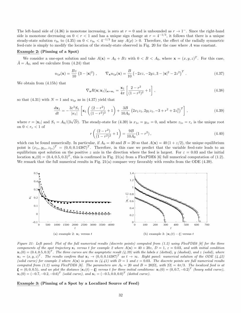
The left-hand side of (4.36) is monotone increasing, is zero at r = 0 and is unbounded as r → 1−. Since the right-handside is monotone decreasing on 0 < r < 1 and has a unique sign change at r = 4−1/3, it follows that there is a uniquesteady-state solution r0e to (4.35) on 0 < r0e < 4−1/3 for any A(ρ) > 0. Therefore, the effect of the radially symmetricfeed-rate is simply to modify the location of the steady-state observed in Fig. 20 for the case where A was constant.

Example 2: (Pinning of a Spot)

We consider a one-spot solution and take A(x) = A0 + Bz with 0 < B < A0, where x = (x, y, z)T . For this case,A = A0, and we calculate from (4.24) that

u1p(x) =Bz

10

(3− |x|2

), ∇xu1p(x) =

B

10

(−2xz,−2yz, 3− |x|2 − 2z2

)T. (4.37)

We obtain from (4.15b) that

∇xR(x; x1)|x=x1 =x1

4π

[2− r2

(1− r2)2+ 1

], (4.38)

so that (4.31) with N = 1 and u1p as in (4.37) yield that

dx1

dt= −3ε3S1

|κ1|

[x1

((2− r2)

(1− r2)2+ 1

)+

3B

10A0

(2x1z1, 2y1z1,−3 + r2 + 2z2

1

)T], (4.39)

where r = |x1| and S1 = A0/(3√D). The steady-state for (4.39) is x1e = y1e = 0, and where z1e = re is the unique root

on 0 < re < 1 of

r

((2− r2)

(1− r2)2+ 1

)=

9B

10A0(1− r2) , (4.40)

which can be found numerically. In particular, if A0 = 40 and B = 20 so that A(x) = 40 (1 + z/2), the unique equilibriumpoint is (x1e, y1e, z1e)

T = (0, 0, 0.14387)T . Therefore, in this case we predict that the variable feed-rate leads to anequilibrium spot solution on the positive z axis in the direction where the feed is largest. For ε = 0.03 and the initiallocation x1(0) = (0.4, 0.5, 0.3)T , this is confirmed in Fig. 21(a) from a FlexPDE6 [6] full numerical computation of (1.2).We remark that the full numerical results in Fig. 21(a) compare very favorably with results from the ODE (4.39).

0 500 1000 1500 2000 2500 3000 3500 4000t

-0.1

0

0.1

0.2

0.3

0.4

0.5

x1

(a) example 2: x1 versus t

0 100 200 300 400 500 600 700t

0

0.2

0.4

0.6

0.8

1

1.2

1.4

|x1−ξ|

(b) example 3: |x1(t)− ξ| versus t

Figure 21: Left panel: Plot of the full numerical results (discrete points) computed from (1.2) using FlexPDE6 [6] for the threecomponents of the spot trajectory x1 versus t for example 2 where A(x) = 40 + 20z, D = 1, ε = 0.03, and with initial conditionx1(0) = (0.4, 0.5, 0.3)T . The three curves are the asymptotic result (4.39) with the labels x (dotted), y (dashed), and z (solid), wherex1 = (x, y, z)T . The results confirm that x1 → (0, 0, 0.14387)T as t → ∞. Right panel: numerical solution of the ODE (4.42)(solid curve) for example 3 where A(x) is given in (4.41) with D = 1 and ε = 0.03. The discrete points are full numerical resultscomputed from (1.2) using FlexPDE6 [6]. The parameters are A0 = 20 and B = 20|Ω|, with |Ω| = 4π/3. The localized feed is atξ = (0, 0, 0.5), and we plot the distance |x1(t)− ξ| versus t for three initial conditions: x1(0) = (0, 0.7,−0.2)T (heavy solid curve),x1(0) = (−0.7,−0.2,−0.6)T (solid curve), and x1 = (−0.5, 0.0, 0.0)T (dotted curve).

Example 3: (Pinning of a Spot by a Localized Source of Feed)

32

Finally, we consider one-spot dynamics for the case where the variable feed-rate has a background state that isaugmented by a localized source where the feed is large. As a model for this situation we take

A(x) = A0 +Bδ(x− ξ) , (4.41)

where A0 > 0, B > 0, and ξ ∈ Ω. We calculate A = A0 + B/|Ω|, and the solution to (4.24) is u1p(x) = BG(x; ξ). From(4.31) and (4.15), we obtain that the one-spot dynamics is

dx1

dt= −3ε3S1

|κ1|

[x1

((2− r2)

(1− r2)2+ 1

)− 3B

A0 +B/|Ω|∇xG(x; ξ)|x=x1

], (4.42)

with S1 = (A0 +B/|Ω|) /(3√D), and where ∇xG(x; ξ)|x=x1

can be calculated from (4.15a). Due to the 1/r singularityin G, it follows from (4.42) that if the initial point x1(0) is sufficiently close to the source ξ of the feed, then we claimthat x1(T ) = ξ at some t = T < ∞. To see this, we observe from (4.42) and (4.15a) that for x1 near ξ, we havedx1/dt ∼ −c(x1 − ξ)/|x1 − ξ|3 for some c > 0, which implies that |x1 − ξ| ∼ (3c)1/3(T − t)1/3 for t near T .

This finite-time pinning phenomena is shown in Fig. 21(b) where we plot the distance |x1(t)−ξ| versus t for a one-spotsolution in the unit ball for the parameter set A0 = 20, B = 20|Ω|, D = 1, and ε = 0.03. In this figure we show a veryfavorable comparison between results computed from the asymptotic ODE (4.42) and the full numerical solution to (1.2)using FlexPDE6 [6] for three different initial conditions x1(0). When using FlexPDE6 on (1.2) for A(x) given in (4.41),we mollified the delta singularity by using the following 3-D Gaussian approximation with σ = 0.005:

A(x) = A0 +BF (|x− ξ|) , where F (|x− ξ|) ≡ (πσ)−3/2 exp(−σ−1|x− ξ|2

).

5 Discussion

We have developed a hybrid asymptotic-numerical approach to analyze the existence, linear stability, and slow dynamicsof quasi-equilibrium N -spot patterns for the singularly perturbed 3-D Schnakenberg model (1.2) in the limit ε → 0. Interms of the original model (1.1), such patterns occur in the large diffusivity regime D = O(ε−4). Our hybrid asymptotic-numerical framework characterizing the linear stability of quasi-equilibrium spot patterns and slow spot dynamics wasimplemented numerically for some spot patterns in the unit ball. Our linear stability results and asymptotic predictionsfor the slow spot dynamics were shown to compare very favorably with results obtained from full numerical simulationsof the 3-D Schnakenberg model (1.2) using FlexPDE6 [6].

We now briefly discuss a few open problems that warrant further study. Our implementation of slow spot dynamicswas done only for the case where Ω is the unit ball, for which there is an explicit analytical formula for the NeumannGreen’s function and its regular part. To leading-order in ε, the slow ODE dynamics in (4.18) for a spatially uniform feedA, and in (4.32) for a variable feed A(x), depend on the gradient of this Neumann Green’s function. For more complicateddomains, it would be interesting to implement the explicit ODE dynamics numerically by using fast multipole methods(cf. [8]) to compute the required Green’s function both accurately and rapidly. Such fast multipole methods would behighly advantageous in this setting, since in simulating the ODE dynamics in (4.18) or (4.32) the gradients of the Green’sfunction must be evaluated at each discrete point of the discretization of the ODE dynamics. With this approach itshould be tractable to numerically study spot-dynamics and, in particular, spot-pinning effects due to either changes inthe domain geometry or spatial variations in the variable feed-rate A(x).

For the case where A > 0 is constant, a second open problem is to identify stable equilibria of the leading-orderODE dynamics (4.18) that have large basins of attraction for initial conditions. As N increases, the energy landscapeof the discrete energy H in (4.17) will have an increasingly large number of local minima with nearly the same energy(cf. [3] and the references therein). These local minima are all linearly stable equilibrium points of (4.18). A naturalquestion is to study, as N increases, whether most initial conditions for (4.18) tend to the global minimum point of H.Our computations of (4.18) for random configurations of spots have suggested that this property holds N = 2, . . . , 20.For the unit ball, the global minimum of H for N = 2, . . . , 20 was computed using numerical optimization software in[3], but it becomes computationally much more challenging to compute it for larger N . Therefore, in what sense can theODE system (4.18) be used as a regularization for computing the global minimum point of H? From a numerical analysisviewpoint, a related ODE regularization was used in [16] to compute a minimum energy configuration for 2-D Coulombparticles on the surface of a ball. We remark that the identification of the global minimum point of H also arises in other

33

contexts. In particular, it corresponds to the spatial configuration of the centers of small traps that minimize the averagemean first passage time for a Brownian walker in a 3-D domain [3] that has a uniformly distributed starting point in thedomain.

A related open question is to identify steady-state spatial configurations of (4.18) for which e = (1, . . . , 1)T is aneigenvector of the Neumann Green’s matrix G. When this condition holds, we determined an improved approximationfor the competition stability threshold in Main Result 3.1 that involves the minimum eigenvalue of G in the subspaceorthogonal to e. In this case, asymmetric spot equilibrium solution branches all bifurcate from the symmetric solutionbranch at a common point. In contrast, if e is not an eigenvector of G at the steady-state of (4.18), we can expect anintricate imperfection-sensitive bifurcation structure near the competition instability threshold. Although we studied thisdelicate behavior analytically near the competition instability threshold for the case N = 2 in (2.44) of §2.1, it is an openissue to locally examine this imperfection sensitivity analytically for larger N .

Finally, we remark that it should be possible to develop a similar hybrid asymptotic-numerical approach to studylocalized quasi-equilibrium spot patterns in a 3-D setting for other well-known singularly perturbed RD systems, such asthe Gierer-Meinhardt, Gray-Scott, and Brusselator models.

Acknowledgments

Theodore Kolokolnikov and Michael Ward were supported by NSERC Discovery grants. Justin Tzou was partiallysupported by a PIMS CRG Postdoctoral Fellowship.

References

[1] I. Barrass, E. J. Crampin, and P. K Maini, Mode transitions in a model reaction–diffusion system driven bydomain growth and noise, Bull. Math. Biol., 68 (2006), pp. 981–995.

[2] W. Chen and M. J. Ward, The stability and dynamics of localized spot patterns in the two-dimensional Gray-Scottmodel, SIAM J. Appl. Dyn. Sys., 10 (2011), pp. 582–666.

[3] A. Cheviakov and M. J. Ward, Optimizing the principal eigenvalue of the Laplacian in a sphere with interiortraps, Math. and Comp. Modeling, 53 (2011), pp. 1394–1409.

[4] E. J. Crampin, E. A. Gaffney, and P. K. Maini, Reaction and diffusion on growing domains: scenarios forrobust pattern formation, Bull. Math. Biol., 61 (1999), pp. 1093–1120.

[5] A. Dhooge, W. Govaerts, and Y. A. Kuznetsov, MATCONT: A MATLAB package for numerical bifurcationanalysis of Odes, ACM Transactions on Mathematical Software (TOMS), 29 (2003), pp. 141–164.

[6] FlexPDE6, PDE Solutions Inc. URL http://www.pdesolutions.com.

[7] E. A. Gaffney and N. A. M. Monk, Gene expression time delays and Turing pattern formation systems, Bull.Math. Bio., 68 (2006), pp. 99–130.

[8] L. Greengard and V. Rokhlin, A new version of the fast multipole method for the laplace equation in threedimensions, Acta Numerica, 6 (1997), pp. 229–269.

[9] D. Iron and M. J. Ward, A metastable spike soluton for a non-local reaction-diffusion model, SIAM J. Appl.Math., 60 (2000), pp. 778–802.

[10] D. Iron, J. Wei, and M. Winter, Stability analysis of Turing patterns generated by the Schnakenberg model, J.Math. Biology, 49 (2004), pp. 358–390.

[11] Theodore Kolokolnikov, Michael J Ward, and Juncheng Wei, The existence and stability of spike equilibriain the one-dimensional gray–scott model: the pulse-splitting regime, Physica D: Nonlinear Phenomena, 202 (2005),pp. 258–293.

34

[12] T. Kolokolnikov, M. J. Ward, and J. Wei, Spot self-replication and dynamics for the Schnakenberg model ina two-dimensional domain, J. Nonlinear Sci., 19 (2009), pp. 1–56.

[13] Y. Nishiura, Far-from Equilibrium dynamics: Translations of mathematical monographs, vol. 209, AMS Publica-tions, Providence, Rhode Island, 2002.

[14] I. Rozada, S. Ruuth, and M. J. Ward, The stability of localized spot patterns for the Brusselator on the sphere,SIAM J. Appl. Dyn. Sys., 13 (2014), pp. 564–627.

[15] J Schnakenberg, Simple chemical reaction systems with limit cycle behaviour, J. Theor. Biol., 81 (1979), pp. 389–400.

[16] W. Stortelder, J. de Swart, and J. Pinter, Finding elliptic Fekete point sets: Two numerical solution ap-proaches, J. Comput. Appl. Math., 130 (1998), pp. 205–216.

[17] W. Sun, M. J. Ward, and R. Russell, The slow dynamics of two-spike solutions for the Gray–Scott and Gierer–Meinhardt systems: Competition and oscillatory instabilities, SIAM J. Appl. Dyn. Sys., 4 (2005), pp. 904–953.

[18] P. Trinh and M. J. Ward, The dynamics of localized spot patterns for reaction-diffusion systems on the sphere,Nonlinearity, 29 (2016), pp. 766–806.

[19] V. K. Vanag and I. R. Epstein, Localized patterns in reaction-diffusion systems, Chaos, 17 (2007), p. 037110.

[20] M. J. Ward and J. Wei, The existence and stability of asymmetric spike patterns for the Schnakenberg model,Studies in Applied Mathematics, 109 (2002), pp. 229–264.

[21] , Hopf bifurcation of spike solutions for the shadow Gierer-Meinhardt model, Europ. J. Appl. Math., 14 (2003),pp. 677–711.

[22] J. Wei and M. Winter, Spikes for the two-dimensional Gierer-Meinhardt system: The weak coupling case, J.Nonlinear Sci., 11 (2001), pp. 415–458.

[23] , Asymmetric spotty patternns for the gray-scott model in R2, Studies in Appl. Math., 110 (2003), pp. 63–102.

[24] , Existence and stability of multiple spot solutions for the Gray-Scott model in R2, Physica D, 176 (2003),pp. 147–180.

[25] , Stationary multiple spots for reaction-diffusion systems, J. Math. Biol., 57 (2008), pp. 53–89.

[26] S. Xie and T. Kolokolnikov, Moving and jumping spot in a two dimensional reaction diffusion model, submitted,Nonlinearity, (2016).

35