
THE OPEN UNIVERSITYFILE/... · THE OPEN UNIVERSITY ... Stage 1, your mathematical knowledge should...
56
THE OPEN UNIVERSITY [Press ↓ to begin]
Transcript of THE OPEN UNIVERSITYFILE/... · THE OPEN UNIVERSITY ... Stage 1, your mathematical knowledge should...

THE OPEN UNIVERSITY
[Press ↓ to begin]
jc34
Typewritten Text
Practical modern statistics (M249) Diagnostic Quiz
jc34
Typewritten Text
© The Open University Last Revision Date: March 2015
jc34
Typewritten Text
Version 4.3
jc34
Typewritten Text
jc34
Typewritten Text
jc34
Typewritten Text
jc34
Typewritten Text
jc34
Typewritten Text
Section 1: Introduction
1. Introduction
Page 2
jc34
Typewritten Text
In order to study Practical modern statistics (M249), it is assumed that you have some knowledge of statistics as well as some basic mathematical skills. This quiz covers a number of key mathematical and statistical areas with which you should be familiar.
jc34
Typewritten Text
For M249 you require a good knowledge of statistical ideas and methods at an introductory level. The statistical prerequisites are revised in the Introduction to statistical modelling (click on link). They include: graphical and numerical data summaries; the basic statistical distributions including the normal, exponential, uniform, binomial and Poisson distributions; confidence intervals and significance tests, correlations and contingency tables. No knowledge of regression is required. If you have taken Analysing data (M248) you should have the required statistical background.
jc34
Typewritten Text
You are also expected to be familiar with mathematical notation, to be able to follow short algebraic arguments, to handle the logarithm and exponential functions, and to use formulas. If you have passed M248, or completed study of mathematics at Stage 1, your mathematical knowledge should be ample. No knowledge of calculus, differentiation or integration is required.
jc34
Typewritten Text
(continued on following page)
Section 1: Introduction Page 3
Try each question for yourself, using your calculator if you wish, then click on the green section letter (e.g. ‘(a)’) to see the solution. Click on the symbol at the end of the solution to return to the question. Use the and keys to move from Section to Section. There is some advice on evaluating your performance at the end of the quiz.
Section 2: Decimals and fractions
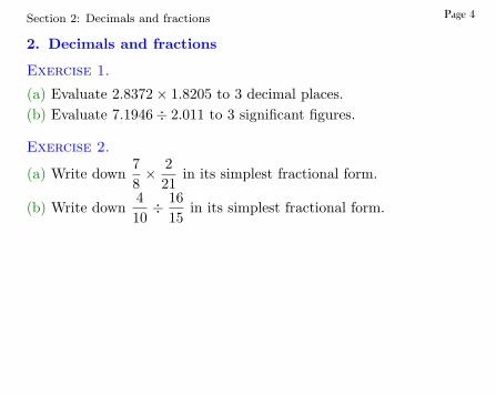
2. Decimals and fractions
Exercise 1.
(a) Evaluate 2.8372× 1.8205 to 3 decimal places.(b) Evaluate 7.1946÷ 2.011 to 3 significant figures.
Exercise 2.
(a) Write down78× 2
21in its simplest fractional form.
(b) Write down410÷ 16
15in its simplest fractional form.
Page 4
Section 3: Formulas and equations
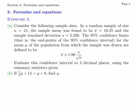
3. Formulas and equations
Exercise 3.
(a) Consider the following sample data. In a random sample of sizen = 15, the sample mean was found to be x = 10.25 and thesample standard deviation s = 2.326. The 95% confidence limits(that is, the end-points of the 95% confidence interval) for themean µ of the population from which the sample was drawn aredefined to be
x± 1.96s√n
Evaluate this confidence interval to 2 decimal places, using thesummary statistics given.
(b) If 52y + 14 = y + 8, find y.
Page 5
Section 4: Powers, logarithms and the exponential function
4. Powers, logarithms and the exponential function
Exercise 4.
(a) Write 33 × 34 in the form 3n and hence evaluate it.(b) Write
(33
)4 in the form 3n and hence evaluate it.(c) Write 34/34 in the form 3n and hence evaluate it.
Exercise 5. This exercise is about logarithms to base e, which aresometimes called ‘natural logarithms’ and may be denoted by ‘ln’,‘loge’ or just ‘log’.(a) To 4 decimal places, log 3 = 1.0986 and log 4 = 1.3863. Without
evaluating any other logarithms, use these values to find log 12 to3 decimal places.
(b) If log x = 1.2, what is x, to 3 decimal places?
Exercise 6.
(a) Suppose that exp (x) = 2, for some number x. Without evaluatingx, use this result to find exp (−x) and exp (2x).
(b) If exp(x) = 3.2, what is x, to 3 decimal places?
Page 6
Section 5: Graphs 1: Bar charts and histograms
5. Graphs 1: Bar charts and histograms
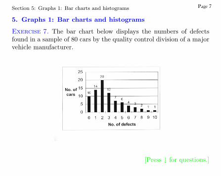
Exercise 7. The bar chart below displays the numbers of defectsfound in a sample of 80 cars by the quality control division of a majorvehicle manufacturer.
[Press ↓ for questions.]
Page 7
Section 5: Graphs 1: Bar charts and histograms
(a) What proportion of cars in the sample have at most 4 faults?(b) What proportion of cars in the sample have between 4 and 6 faults
inclusive?(c) Without performing any calculations, would you expect the sample
mean number of faults to be greater than the sample median?Give a reason for your answer.
[Press ↑ to return to graph.][Press ↓ for next exercise.]
Page 8
Section 6: Graphs 2: Scatterplots
6. Graphs 2: Scatterplots
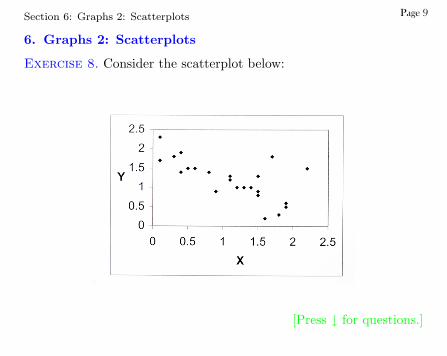
Exercise 8. Consider the scatterplot below:
[Press ↓ for questions.]
Page 9
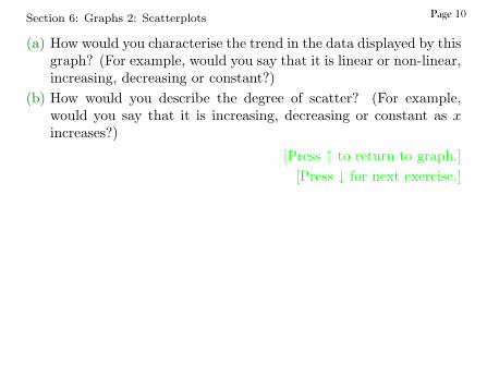
Section 6: Graphs 2: Scatterplots
(a) How would you characterise the trend in the data displayed by thisgraph? (For example, would you say that it is linear or non-linear,increasing, decreasing or constant?)
(b) How would you describe the degree of scatter? (For example,would you say that it is increasing, decreasing or constant as xincreases?)
[Press ↑ to return to graph.][Press ↓ for next exercise.]
Page 10
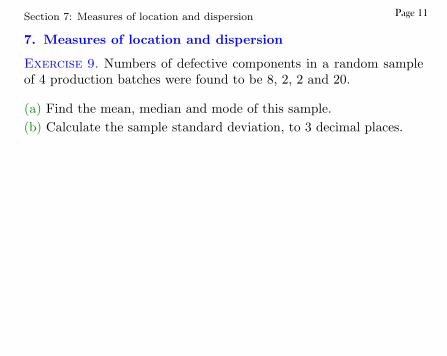
Section 7: Measures of location and dispersion
7. Measures of location and dispersion
Exercise 9. Numbers of defective components in a random sampleof 4 production batches were found to be 8, 2, 2 and 20.
(a) Find the mean, median and mode of this sample.(b) Calculate the sample standard deviation, to 3 decimal places.
Page 11
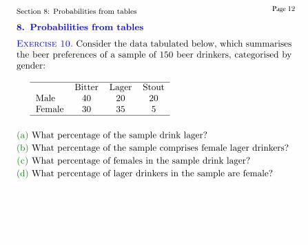
Section 8: Probabilities from tables
8. Probabilities from tables
Exercise 10. Consider the data tabulated below, which summarisesthe beer preferences of a sample of 150 beer drinkers, categorised bygender:
Bitter Lager StoutMale 40 20 20Female 30 35 5
(a) What percentage of the sample drink lager?(b) What percentage of the sample comprises female lager drinkers?(c) What percentage of females in the sample drink lager?(d) What percentage of lager drinkers in the sample are female?
Page 12
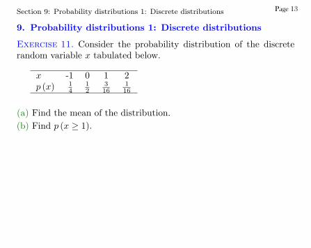
Section 9: Probability distributions 1: Discrete distributions
9. Probability distributions 1: Discrete distributions
Exercise 11. Consider the probability distribution of the discreterandom variable x tabulated below.
x -1 0 1 2p (x) 1
412
316
116
(a) Find the mean of the distribution.(b) Find p (x ≥ 1).
Page 13
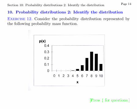
Section 10: Probability distributions 2: Identify the distribution
10. Probability distributions 2: Identify the distribution
Exercise 12. Consider the probability distribution represented bythe following probability mass function.
[Press ↓ for questions.]
Page 14
Section 10: Probability distributions 2: Identify the distribution
Do you think that this probability mass function (p.m.f.) represents:
(a) a normal distribution?(b) a binomial distribution?(c) a Poisson distribution?
[Press ↑ to return to graph.][Press ↓ for next exercise.]
Page 15
Section 11: Hypothesis testing
11. Hypothesis testing
Exercise 13. A hypothesis test has been undertaken to test the nullhypothesis that there is no difference between the proportions of girlsand boys who get a grade ‘A’ in GCSE Mathematics. The significanceprobability (or p value) was found to be be 0.0034.
(a) Which of the following two statements is true?
(A) ‘There is strong evidence that the underlyingproportions are the same.’
OR
(B) ‘There is strong evidence that the underlyingproportions are not the same.’
Page 16
Section 12: Confidence intervals
12. Confidence intervals
Exercise 14. Suppose that (−2.6, 3.4) is a 95% confidence intervalfor some parameter θ.
Classify the following statements as true or false:
(a) 3.3 lies outside the corresponding 99% confidence interval for θ.(b) On the basis of these data, it is very implausible that θ should
equal zero.
Page 17
Section 13: Correlation
13. Correlation
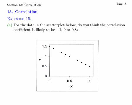
Exercise 15.
(a) For the data in the scatterplot below, do you think the correlationcoefficient is likely to be −1, 0 or 0.8?
Page 18
Section 13: Correlation
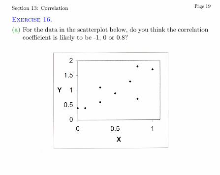
Exercise 16.
(a) For the data in the scatterplot below, do you think the correlationcoefficient is likely to be -1, 0 or 0.8?
Page 19
Section 13: Correlation
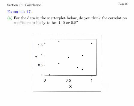
Exercise 17.
(a) For the data in the scatterplot below, do you think the correlationcoefficient is likely to be -1, 0 or 0.8?
Page 20
Section 14: Post-mortem
14. Post-mortem
Page 21
jc34
Typewritten Text
If you had difficulty in answering some of these questions, you might find it useful to look at the pre-registration version of the Introduction to statistical modelling, (click on link) which comprises a revision of the pre-requisites for M249. You should only attempt to read Sections 1, 3, 4 and 5; Sections 2 and 6 introduce the statistical package SPSS which you will not receive until you have registered for the course. (If you decide to study M249, you will need to work through this unit again, including the computing sections.) If you found the mathematics exercises 1 - 6 difficult, you might consider studying one of the mathematics entry level modules, MU123 or MST124, before embarking on M249. On the other hand, if you found the statistics exercises 7 - 17 difficult, you would be advised to study Analysing data (M248) before M249. If you have any queries about your suitability for the course, you should contact your Student Support Team via StudentHome.
jc34
Typewritten Text
jc34
Typewritten Text
jc34
Typewritten Text
Solutions to Exercises
Solutions to Exercises
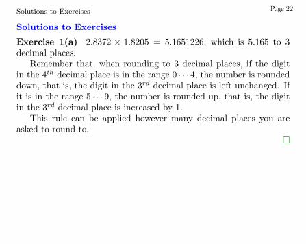
Exercise 1(a) 2.8372 × 1.8205 = 5.1651226, which is 5.165 to 3decimal places.
Remember that, when rounding to 3 decimal places, if the digitin the 4th decimal place is in the range 0 · · · 4, the number is roundeddown, that is, the digit in the 3rd decimal place is left unchanged. Ifit is in the range 5 · · · 9, the number is rounded up, that is, the digitin the 3rd decimal place is increased by 1.
This rule can be applied however many decimal places you areasked to round to.
�
Page 22
Solutions to Exercises
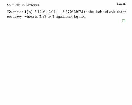
Exercise 1(b) 7.1946÷2.011 = 3.577623073 to the limits of calculatoraccuracy, which is 3.58 to 3 significant figures.
�
Page 23
Solutions to Exercises
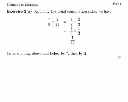
Exercise 2(a) Applying the usual cancellation rules, we have
78× 2
21=
18× 2
3
=14× 1
3
=112
(after dividing above and below by 7, then by 2).�
Page 24
Solutions to Exercises
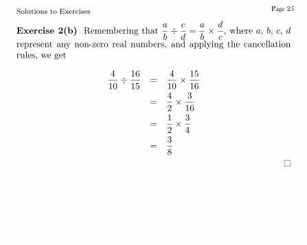
Exercise 2(b) Remembering thata
b÷ c
d=
a
b× d
c, where a, b, c, d
represent any non-zero real numbers, and applying the cancellationrules, we get
410÷ 16
15=
410× 15
16
=42× 3
16
=12× 3
4
=38
�
Page 25
Solutions to Exercises
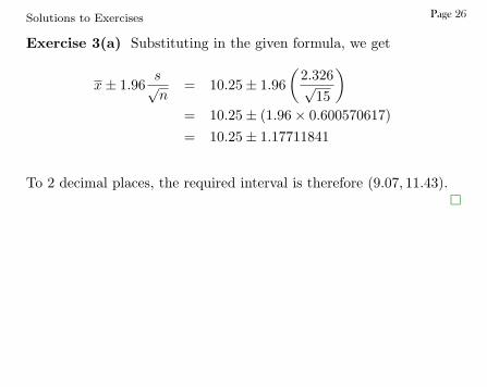
Exercise 3(a) Substituting in the given formula, we get
x± 1.96s√n
= 10.25± 1.96(
2.326√15
)= 10.25± (1.96× 0.600570617)= 10.25± 1.17711841
To 2 decimal places, the required interval is therefore (9.07, 11.43).�
Page 26
Solutions to Exercises
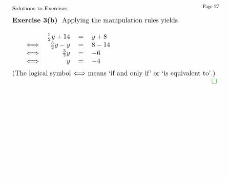
Exercise 3(b) Applying the manipulation rules yields
52y + 14 = y + 8
⇐⇒ 52y − y = 8− 14
⇐⇒ 32y = −6
⇐⇒ y = −4
(The logical symbol ⇐⇒ means ‘if and only if’ or ‘is equivalent to’.)�
Page 27
Solutions to Exercises
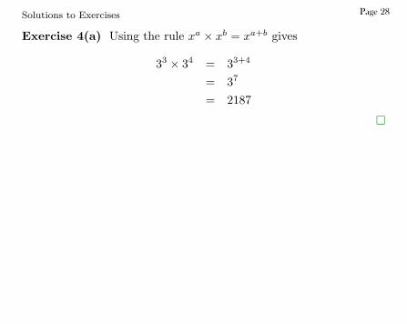
Exercise 4(a) Using the rule xa × xb = xa+b gives
33 × 34 = 33+4
= 37
= 2187
�
Page 28
Solutions to Exercises
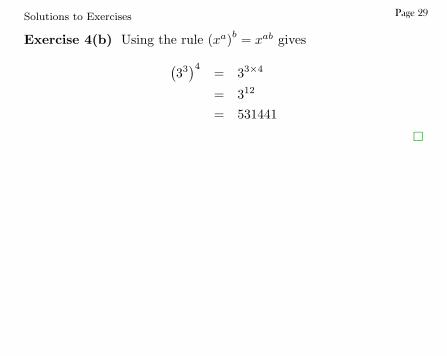
Exercise 4(b) Using the rule (xa)b = xab gives(33
)4= 33×4
= 312
= 531441
�
Page 29
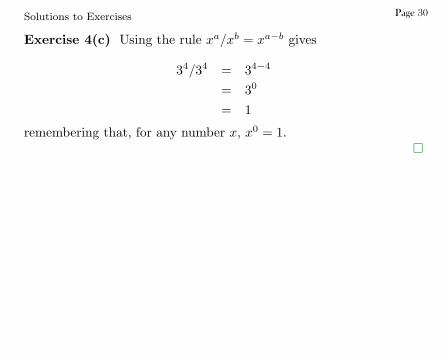
Solutions to Exercises
Exercise 4(c) Using the rule xa/xb = xa−b gives
34/34 = 34−4
= 30
= 1
remembering that, for any number x, x0 = 1.�
Page 30
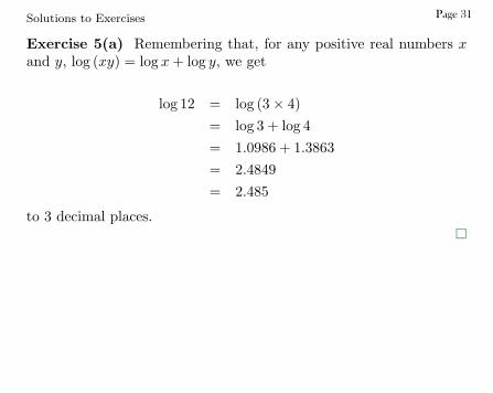
Solutions to Exercises
Exercise 5(a) Remembering that, for any positive real numbers xand y, log (xy) = log x + log y, we get
log 12 = log (3× 4)= log 3 + log 4= 1.0986 + 1.3863= 2.4849= 2.485
to 3 decimal places.�
Page 31
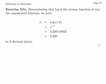
Solutions to Exercises
Exercise 5(b) Remembering that log is the inverse function of exp,the exponential function, we have
x = exp (1.2)= e1.2
= 3.320116923= 3.320
to 3 decimal places.�
Page 32
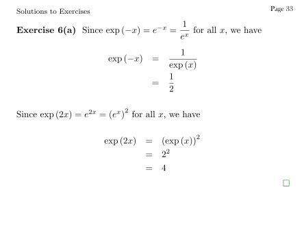
Solutions to Exercises
Exercise 6(a) Since exp (−x) = e−x =1ex
for all x, we have
exp (−x) =1
exp (x)
=12
Since exp (2x) = e2x = (ex)2 for all x, we have
exp (2x) = (exp (x))2
= 22
= 4
�
Page 33
Solutions to Exercises
Exercise 6(b) Again remembering that log is the inverse functionof exp, we have
x = log (3.2)= 1.16315081= 1.163
to 3 decimal places.�
Page 34
Solutions to Exercises
Exercise 7(a) The number of cars with at most 4 faults is
10 + 14 + 20 + 12 + 7 = 63.
The proportion is therefore 6380∼= 0.79.
�
Page 35
Solutions to Exercises
Exercise 7(b) The number of cars with between 4 and 6 faultsinclusive is 7 + 6 + 4 = 17. The proportion is therefore 17
80∼= 0.21.
�
Page 36
Solutions to Exercises
Exercise 7(c) Yes. For right-skew data, the sample mean is greaterthan the sample median.
�
Page 37
Solutions to Exercises
Exercise 8(a) A visual inspection suggests that x and y could wellbe linearly related. y appears to be decreasing as x increases.
�
Page 38
Solutions to Exercises
Exercise 8(b) The degree of scatter appears to be increasing as xincreases.
�
Page 39
Solutions to Exercises
Exercise 9(a) The mean is 8+2+2+204 = 8.
The ordered sample is 2, 2, 8, 20, so the median is 2+82 = 5.
The mode is the most frequently-occurring value, in this case 2.�
Page 40
Solutions to Exercises
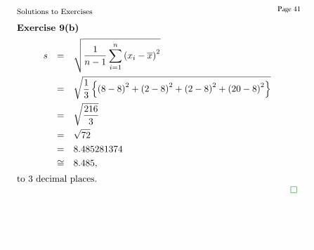
Exercise 9(b)
s =
√√√√ 1n− 1
n∑i=1
(xi − x)2
=
√13
{(8− 8)2 + (2− 8)2 + (2− 8)2 + (20− 8)2
}=
√2163
=√
72= 8.485281374∼= 8.485,
to 3 decimal places.�
Page 41
Solutions to Exercises
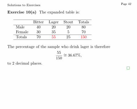
Exercise 10(a) The expanded table is:
Bitter Lager Stout TotalsMale 40 20 20 80Female 30 35 5 70Totals 70 55 25 150
The percentage of the sample who drink lager is therefore55150
∼= 36.67%,
to 2 decimal places.�
Page 42
Solutions to Exercises
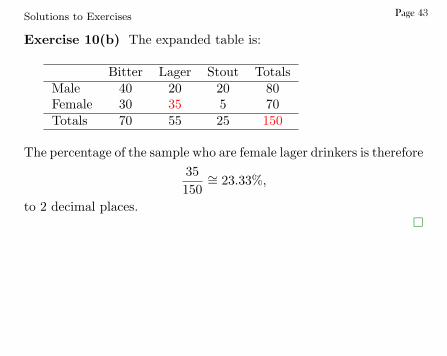
Exercise 10(b) The expanded table is:
Bitter Lager Stout TotalsMale 40 20 20 80Female 30 35 5 70Totals 70 55 25 150
The percentage of the sample who are female lager drinkers is therefore35150
∼= 23.33%,
to 2 decimal places.�
Page 43
Solutions to Exercises
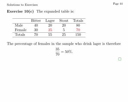
Exercise 10(c) The expanded table is:
Bitter Lager Stout TotalsMale 40 20 20 80Female 30 35 5 70Totals 70 55 25 150
The percentage of females in the sample who drink lager is therefore3570
= 50%.
�
Page 44
Solutions to Exercises
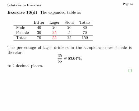
Exercise 10(d) The expanded table is:
Bitter Lager Stout TotalsMale 40 20 20 80Female 30 35 5 70Totals 70 55 25 150
The percentage of lager drinkers in the sample who are female istherefore
3555∼= 63.64%,
to 2 decimal places.�
Page 45
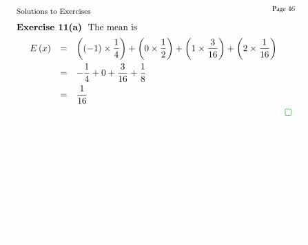
Solutions to Exercises
Exercise 11(a) The mean is
E (x) =(
(−1)× 14
)+
(0× 1
2
)+
(1× 3
16
)+
(2× 1
16
)= −1
4+ 0 +
316
+18
=116
�
Page 46
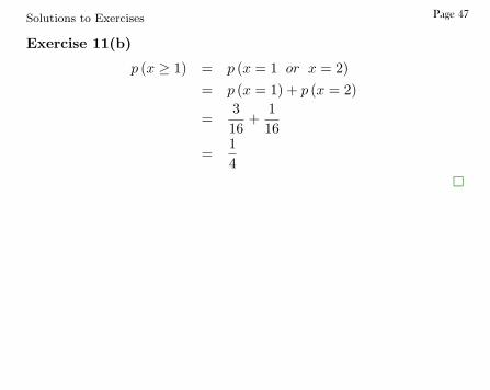
Solutions to Exercises
Exercise 11(b)
p (x ≥ 1) = p (x = 1 or x = 2)= p (x = 1) + p (x = 2)
=316
+116
=14
�
Page 47
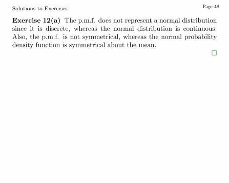
Solutions to Exercises
Exercise 12(a) The p.m.f. does not represent a normal distributionsince it is discrete, whereas the normal distribution is continuous.Also, the p.m.f. is not symmetrical, whereas the normal probabilitydensity function is symmetrical about the mean.
�
Page 48
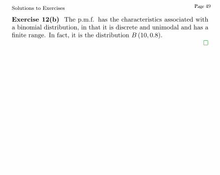
Solutions to Exercises
Exercise 12(b) The p.m.f. has the characteristics associated witha binomial distribution, in that it is discrete and unimodal and has afinite range. In fact, it is the distribution B (10, 0.8).
�
Page 49
Solutions to Exercises
Exercise 12(c) The p.m.f. does not represent a Poisson distributionsince the Poisson distribution is right-skew.
�
Page 50
Solutions to Exercises
Exercise 13(a) The significance probability is the probability ofobtaining data which are at least as extreme as those observed if thenull hypothesis were true. This probability is very small and so wehave strong evidence against the null hypothesis. It is highly unlikelythat the underlying proportions are the same. Thus statement (A) isincorrect and statement (B) is correct.
�
Page 51
Solutions to Exercises
Exercise 14(a) The statement is false. The 99% confidence intervalfor θ is centred on the same value (in this case 0.4) as the 95%confidence interval and is wider. So, since 3.3 lies inside the 95%confidence interval, it must also lie inside the 99% confidence interval.
�
Page 52

Solutions to Exercises
Exercise 14(b) The statement is false. The 95% confidence intervalgives a range of values of θ which are plausible at the 95% confidencelevel. Since this interval contains zero, it is plausible that θ = 0.
�
Page 53
Solutions to Exercises
Exercise 15(a) The data points lie on a straight line with negativegradient. The correlation coefficient is −1.
�
Page 54
Solutions to Exercises
Exercise 16(a) The data points appear to lie fairly close to a straightline with positive gradient. A correlation coefficient of 0.8 would beappropriate here.
�
Page 55

Solutions to Exercises
Exercise 17(a) There appears to be no evidence of any linear trendin these data. A correlation coefficient of 0 would be appropriate here.
�
Page 56