
The Jena regional inversion system: recent developments ...
24
The Jena regional inversion system: recent developments and results Christoph Gerbig, Panagiotis Kountouris, Christian Rödenbeck (MPI-BGC, Jena) Thomas Koch (DWD), Ute Karstens (ICOS-CP, Lund) ICOS-CP workshop June 20-22 2016, Lund
Transcript of The Jena regional inversion system: recent developments ...
TheJenaregionalinversionsystem:recentdevelopmentsandresults
Christoph Gerbig, Panagiotis Kountouris, Christian Rödenbeck (MPI-BGC, Jena)
Thomas Koch (DWD),Ute Karstens (ICOS-CP, Lund)
ICOS-CP workshopJune 20-22 2016, Lund
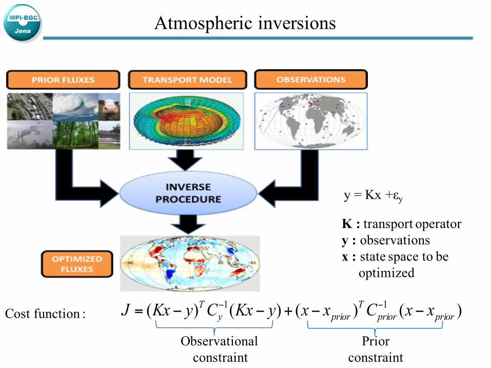
y = Kx +εy
K : transport operatory : observationsx : state space to be
optimized
)()()()( 11priorprior
Tpriory
T xxCxxyKxCyKxJ −−+−−= −−Cost function :
Observationalconstraint
Atmospheric inversions
Priorconstraint
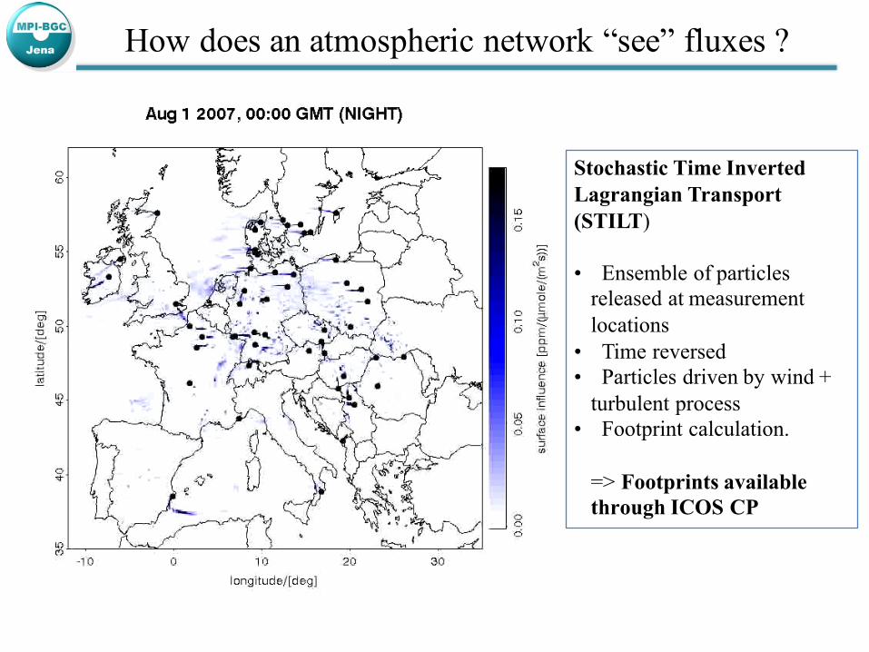
How does an atmospheric network “see” fluxes ?
Stochastic Time Inverted Lagrangian Transport (STILT)
• Ensemble of particlesreleased at measurementlocations
• Time reversed• Particles driven by wind +
turbulent process• Footprint calculation.
=> Footprints available through ICOS CP
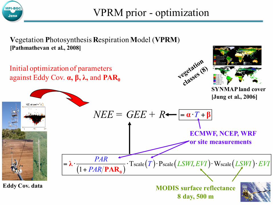
VPRM prior - optimization
Vegetation Photosynthesis Respiration Model (VPRM)[Pathmathevan et al., 2008]
( )( ) ( ) ( )scale scale scaleT P W
1LSWI EVPAR T I L
PS
R, V
AWI E I= ⋅ ⋅ ⋅ ⋅ ⋅
+ 0
λPAR
NEE = GEE + R
SYNMAP land cover[Jung et al., 2006]
Eddy Cov. data
Initial optimization of parametersagainst Eddy Cov. α, β, λ, and PAR0
= ⋅ +Tα β
ECMWF, NCEP, WRFor site measurements
MODIS surface reflectance8 day, 500 m
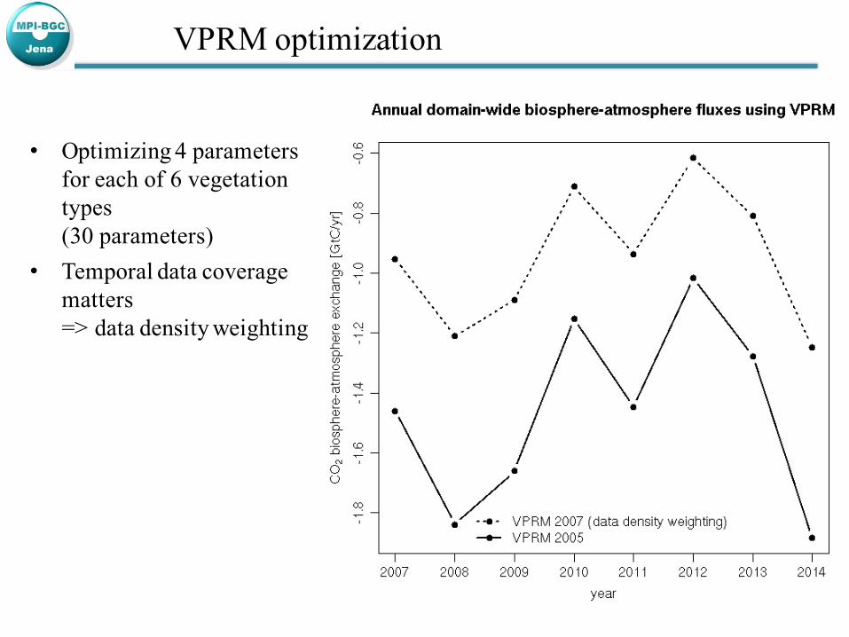
VPRM optimization
• Optimizing 4 parameters for each of 6 vegetation types (30 parameters)
• Temporal data coveragematters=> data density weighting
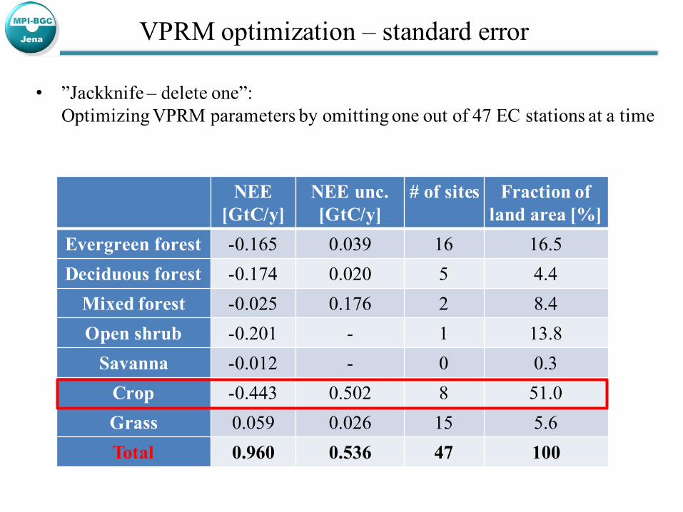
VPRM optimization – standard error
• ”Jackknife – delete one”:Optimizing VPRM parameters by omitting one out of 47 EC stations at a time
NEE[GtC/y]
NEE unc. [GtC/y]
# of sites Fraction of land area [%]
Evergreen forest -0.165 0.039 16 16.5Deciduous forest -0.174 0.020 5 4.4
Mixed forest -0.025 0.176 2 8.4Open shrub -0.201 - 1 13.8
Savanna -0.012 - 0 0.3Crop -0.443 0.502 8 51.0Grass 0.059 0.026 15 5.6Total 0.960 0.536 47 100

Fossil fuel priors
• EDGAR v4.1 at 0.1º
• IPCC category and fuel type differentiation
• Time factors applied to create hourly temporal resolution
• Interannual variations scaled according to BP energy statistics at national level
• Extrapolation to 1-2 yearsafter BP statistics=> current year available

TM3-STILT – two step inversion
• Input : Atmospheric observations, prior fluxes (biospheric, ocean, fossil fuel)
• TM3 global inversion 5° x 4°• STILT regional inversion
0.25° x 0.25°• State space: 0.5° resolution,
3hourly flux optimization
Jena regional inversion system
Rödenbeck et al., 2009
9
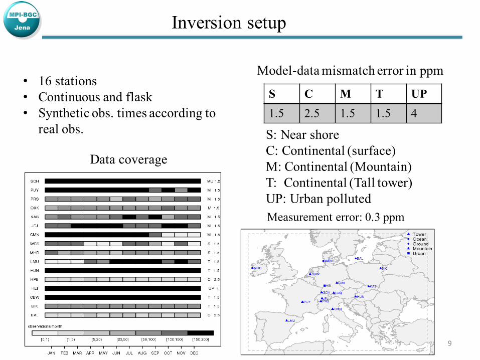
Data coverage
S C M T UP1.5 2.5 1.5 1.5 4
S: Near shoreC: Continental (surface)M: Continental (Mountain)T: Continental (Tall tower)UP: Urban polluted
Model-data mismatch error in ppm
Measurement error: 0.3 ppm
• 16 stations• Continuous and flask• Synthetic obs. times according to
real obs.
Inversion setup
• Data driven error structure• 30 days, 100 km error correlations
=> error inflation needed to obtain 0.3 GtC/yr for annual and domain aggregated prior error (to be consistent with global inversions)
• Sensitivity tests on the error structure
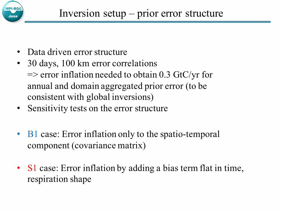
Inversion setup – prior error structure
• B1 case: Error inflation only to the spatio-temporal component (covariance matrix)
• S1 case: Error inflation by adding a bias term flat in time, respiration shape
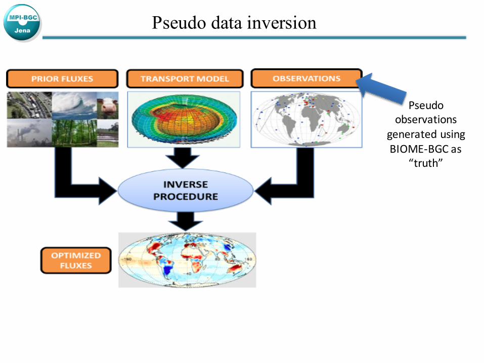
Pseudo data inversion
Pseudoobservations
generatedusingBIOME-BGCas
“truth”
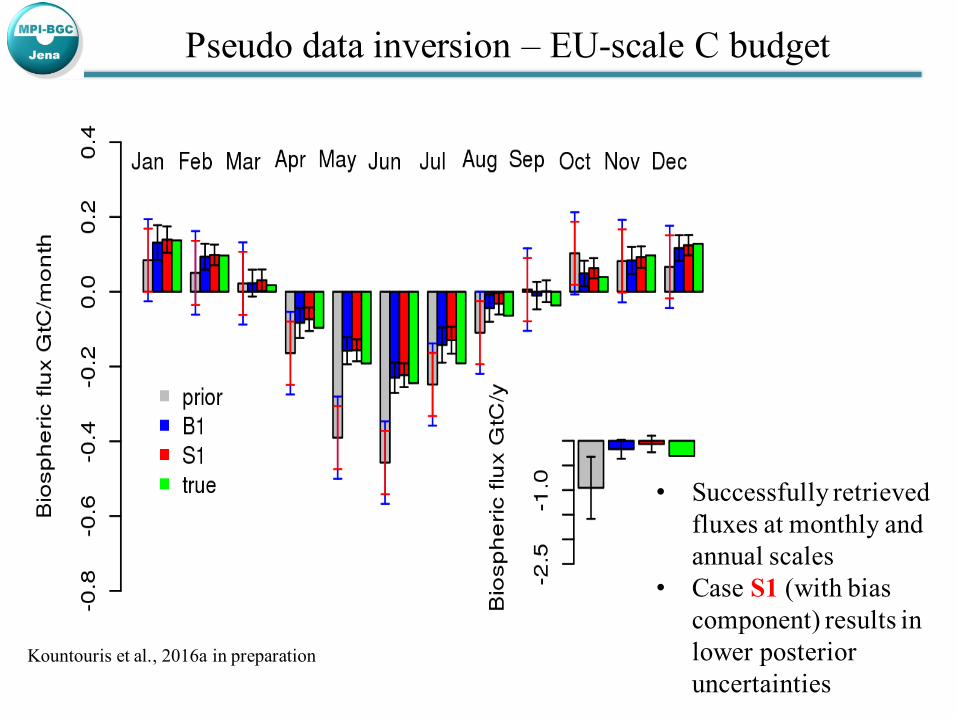
Pseudo data inversion – EU-scale C budget
• Successfully retrieved fluxes at monthly and annual scales
• Case S1 (with bias component) results in lower posterior uncertainties
Kountouris et al., 2016a in preparation
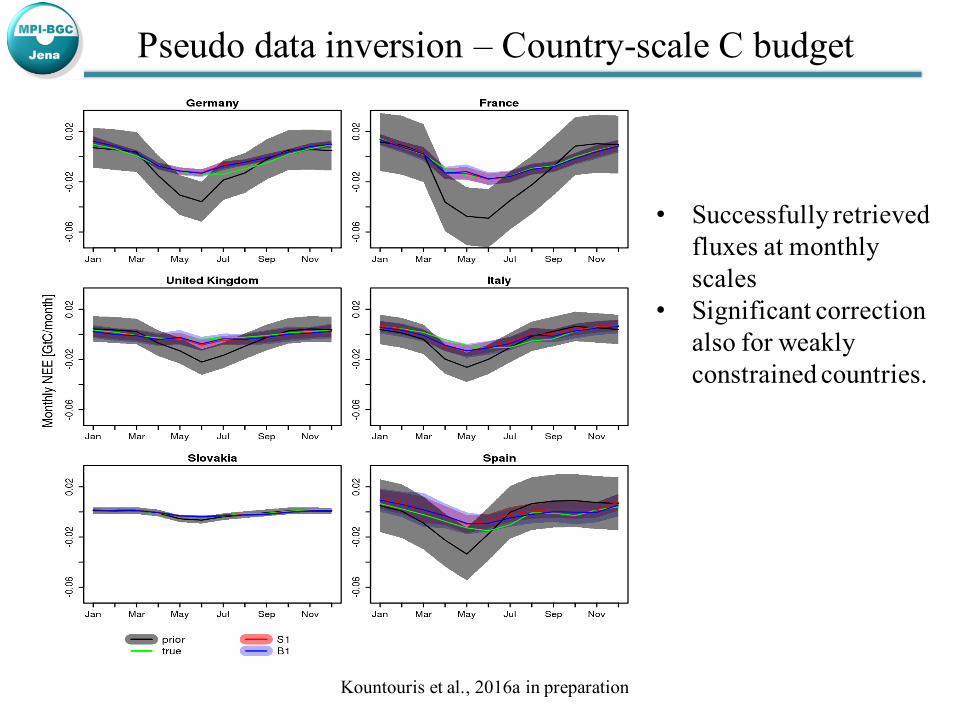
Pseudo data inversion – Country-scale C budget
• Successfully retrieved fluxes at monthly scales
• Significant correction also for weakly constrained countries.
Kountouris et al., 2016a in preparation
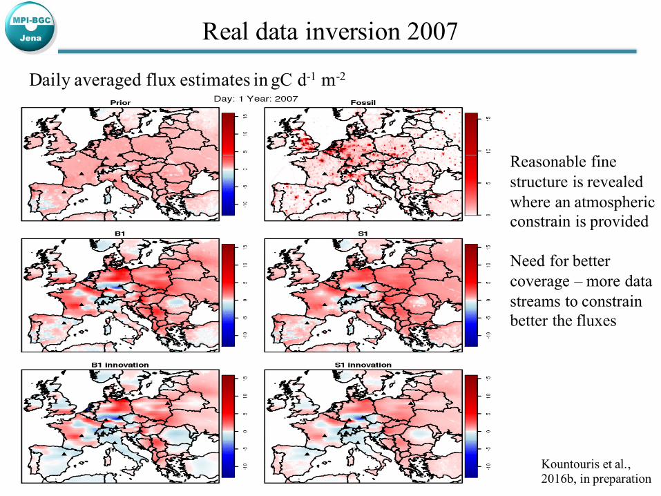
Real data inversion 2007
Daily averaged flux estimates in gC d-1 m-2
• Reasonable fine structure is revealed where an atmospheric constrain is provided
• Need for better coverage – more data streams to constrain better the fluxes
Kountouris et al., 2016b, in preparation
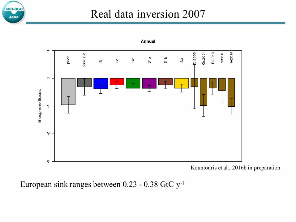
Real data inversion 2007
European sink ranges between 0.23 - 0.38 GtC y-1
Kountouris et al., 2016b in preparation
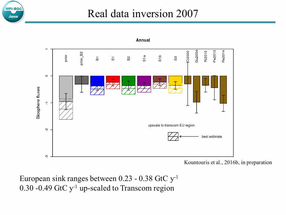
Real data inversion 2007
Kountouris et al., 2016b, in preparation
European sink ranges between 0.23 - 0.38 GtC y-1
0.30 -0.49 GtC y-1 up-scaled to Transcom region
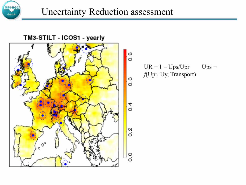
Uncertainty Reduction assessment
UR = 1 – Ups/Upr Ups = f(Upr, Uy, Transport)
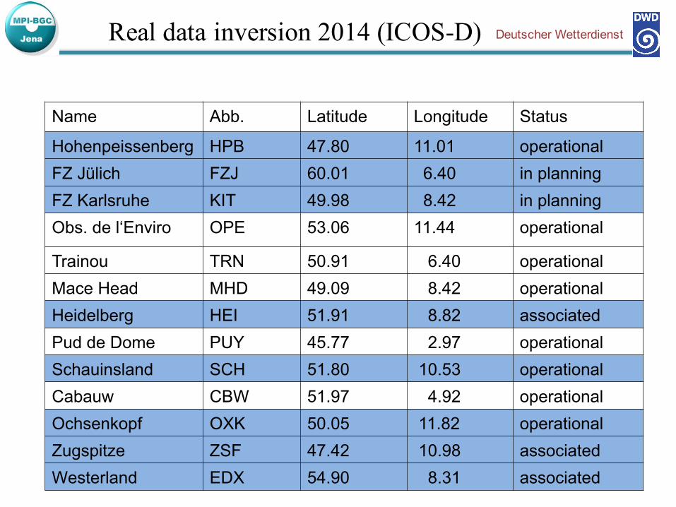
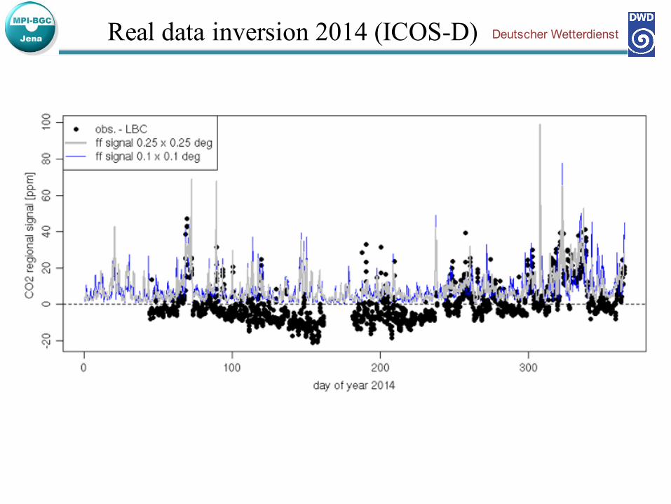
Real data inversion 2014 (ICOS-D)
Name Abb. Latitude Longitude Status
Hohenpeissenberg HPB 47.80 11.01 operationalFZ Jülich FZJ 60.01 6.40 in planningFZ Karlsruhe KIT 49.98 8.42 in planningObs. de l‘Enviro OPE 53.06 11.44 operational
Trainou TRN 50.91 6.40 operationalMace Head MHD 49.09 8.42 operationalHeidelberg HEI 51.91 8.82 associatedPud de Dome PUY 45.77 2.97 operationalSchauinsland SCH 51.80 10.53 operationalCabauw CBW 51.97 4.92 operationalOchsenkopf OXK 50.05 11.82 operationalZugspitze ZSF 47.42 10.98 associatedWesterland EDX 54.90 8.31 associated
Deutscher Wetterdienst
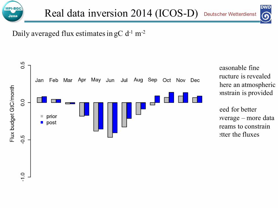
Real data inversion 2014 (ICOS-D)
Daily averaged flux estimates in gC d-1 m-2
• Reasonable fine structure is revealed where an atmospheric constrain is provided
• Need for better coverage – more data streams to constrain better the fluxes
Deutscher Wetterdienst
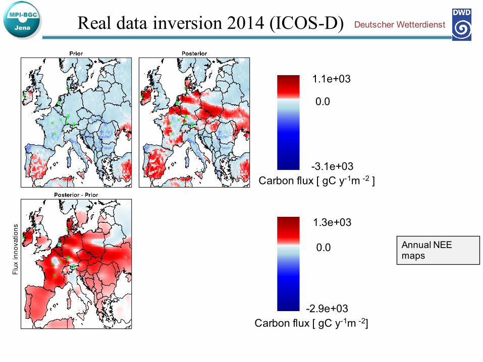
Real data inversion 2014 (ICOS-D)
Daily averaged flux estimates in gC d-1 m-2
Carbon flux [ gC y-1m -2 ]
Carbon flux [ gC y-1m -2]
1.3e+03
1.1e+03
-3.1e+03
-2.9e+03
0.0
0.0
Deutscher Wetterdienst
Annual NEE maps
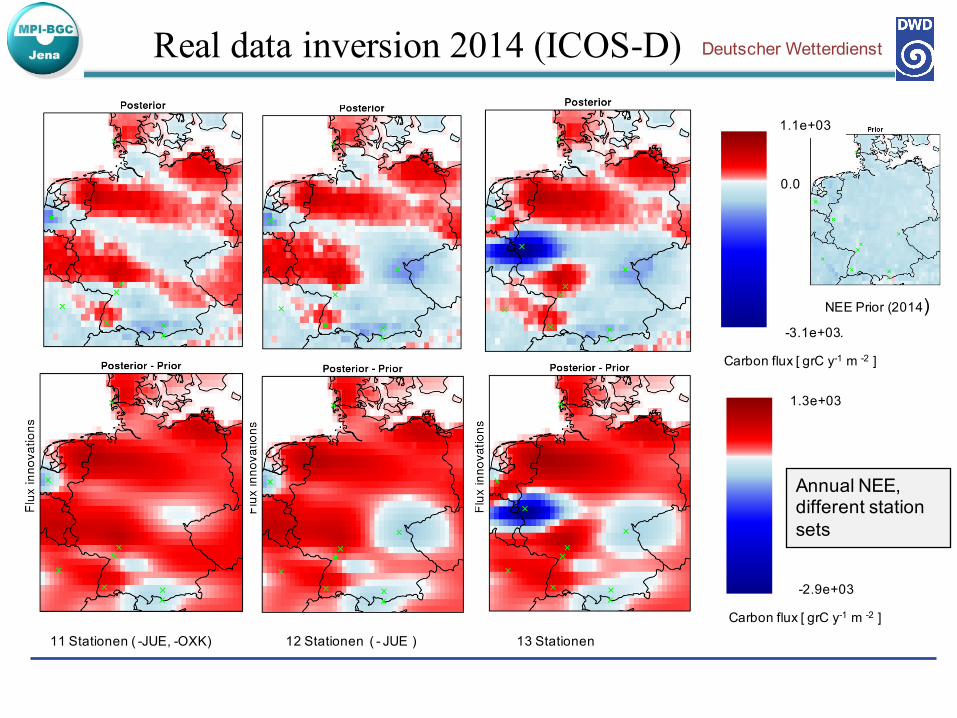
Real data inversion 2014 (ICOS-D)
NEE Prior (2014)-3.1e+03.
1.3e+03
-2.9e+03
Carbon flux [ grC y-1 m -2 ]
Carbon flux [ grC y-1 m -2 ]
11 Stationen ( -JUE, -OXK) 13 Stationen12 Stationen ( - JUE )
Annual NEE, different stationsets
0.0
1.1e+03
Deutscher Wetterdienst
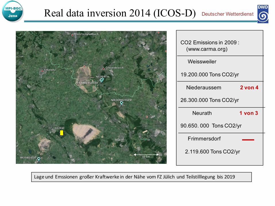
Real data inversion 2014 (ICOS-D)
CO2 Emissions in 2009 :(www.carma.org)
Weissweiler
19.200.000 Tons CO2/yr
Niederaussem 2 von 4
26.300.000 Tons CO2/yr
Neurath 1 von 3
90.650. 000 Tons CO2/yr
Frimmersdorf
2.119.600 Tons CO2/yr
Lageund Emssionen großerKraftwerkeinderNähevomFZJülich undTeilstilllegungbis2019
10 km
Deutscher Wetterdienst
Real data inversion 2014 (ICOS-D) Deutscher Wetterdienst
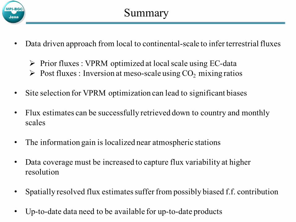
Summary
• Data driven approach from local to continental-scale to infer terrestrial fluxes
Ø Prior fluxes : VPRM optimized at local scale using EC-dataØ Post fluxes : Inversion at meso-scale using CO2 mixing ratios
• Site selection for VPRM optimization can lead to significant biases
• Flux estimates can be successfully retrieved down to country and monthly scales
• The information gain is localized near atmospheric stations
• Data coverage must be increased to capture flux variability at higher resolution
• Spatially resolved flux estimates suffer from possibly biased f.f. contribution
• Up-to-date data need to be available for up-to-date products