The Framework of α-Molecules: Theory and Applications · location, and a certain orientation, and...
266
The Framework of α-Molecules Theory and Applications vorgelegt von Diplom-Mathematiker Martin Schäfer geb. in Köln Von der Fakultät II - Mathematik und Naturwissenschaften der Technischen Universität Berlin zur Erlangung des akademischen Grades Doktor der Naturwissenschaften Dr. rer. nat. genehmigte Dissertation Promotionsausschuss: Vorsitzender: Prof. Dr. Wolfgang König Gutachterin: Prof. Dr. Gitta Kutyniok Gutachterin: Prof. Dr. Gerlind Plonka-Hoch Gutachter: Prof. Dr. Martin Ehler Tag der wissenschaftlichen Aussprache: 17. September 2018 Berlin 2018
Transcript of The Framework of α-Molecules: Theory and Applications · location, and a certain orientation, and...
The Framework of α-MoleculesTheory and Applications
vorgelegt vonDiplom-Mathematiker Martin Schäfer
geb. in Köln
Von der Fakultät II - Mathematik und Naturwissenschaftender Technischen Universität Berlin
zur Erlangung des akademischen Grades
Doktor der NaturwissenschaftenDr. rer. nat.
genehmigte Dissertation
Promotionsausschuss:
Vorsitzender: Prof. Dr. Wolfgang KönigGutachterin: Prof. Dr. Gitta KutyniokGutachterin: Prof. Dr. Gerlind Plonka-HochGutachter: Prof. Dr. Martin Ehler
Tag der wissenschaftlichen Aussprache: 17. September 2018
Berlin 2018

Deutsche Zusammenfassung
Waveletsysteme sind heutzutage ein integraler Bestandteil der harmonischen Analysis unddienen zum Beispiel als effizientes Werkzeug zur Darstellung und Approximation von Si-gnalen. Ihr großer Erfolg beruht dabei unter anderem auf der Fähigkeit, glatte Signale mitlokalen Singularitäten besser zu approximieren als es traditionelle Fouriersysteme können.Bei isotropen Daten, welche insbesondere univariate Signale miteinschließen, ist ihre Per-formanz bei entsprechender Regularität sogar quasi-optimal.
Für die Approximation multivariater Daten hingegen sind Wavelets im allgemeinen nichtoptimal geeignet. Der Grund hierfür liegt in ihrer isotropen Skalierung, die keine optima-le Auflösung anisotroper Strukturen erlaubt. Da solche Strukturen für multivariate Datenjedoch sehr typisch sind – man denke nur an Kanten in Bilddaten zum Beispiel – sind inden letzten Jahre viele Anstrengungen unternommen worden, um diese Unzulänglichkeitzu überwinden. Insbesondere wurden viele neuartige sogenannte direktionale Repräsentati-onssysteme eingeführt, von denen wir als einige der bekanntesten Ridgelets, Curvelets undShearlets nennen wollen.
Solche direktionalen Systeme lassen sich anhand der ihnen zugrundeliegenden Skalierungkategorisieren. Wavelets zum Beispiel sind isotroper Natur, eine rein direktionale Skalierungfindet bei Ridgelets Verwendung, die Konstruktion klassischer Curvelets und Shearlets ba-siert auf einer parabolischen Skalierung. Eine Vielzahl unterschiedlicher Skalierungstypenwird durch das Konzept der α-Skalierung abgedeckt, wo mit Hilfe eines Parameters α ∈ [0, 1]zwischen dem isotropen und dem direktionalen Fall interpoliert wird. Die vorgenannten Sys-teme zum Beispiel sind α-skaliert mit zugehörigen Parametern α = 1, α = 0 und α = 1
2 .Das Hauptziel dieser Dissertation besteht darin, eine einheitliche Theorie für derartige
α-skalierte Repräsentationssysteme zu entwickeln. Den grundlegenden Begriff bilden dabeisogenannte α-Moleküle, die eine Weiterentwicklung des Konzepts der parabolischen Mo-leküle darstellen. Letztere wurden eingeführt, um eine simultane Behandlung parabolischskalierter Systeme zu ermöglichen.
Per Definition entstehen sie durch parabolische Skalierung sowie durch Rotation undTranslation aus einer Menge generierender Funktionen, für die lediglich eine gemeinsameZeit-Frequenz-Lokalisierung gefordert wird. Die Bezeichnung „Molekül“ rührt dabei vonder möglichen Variabilität der Generatoren her. Zusammen mit der Verwendung sogenann-ter Parametrisierungen, welche eine generische Indizierung ermöglichen, bringt diese dienötige Flexibilität in die Konstruktion, um verschiedenartige parabolisch skalierter Sys-teme einheitlich zu beschreiben. Tatsächlich ist das Konzept allgemein genug, um sowohlrotations-basierte als auch scherungs-basierte Systeme wie die klassischen Curvelets und dieklassischen Shearlets zu umfassen.
Nach dem Vorbild parabolischer Molekülsysteme werden auch α-Molekülsysteme mittelsDilatation, Rotation und Translation aus einer zugrundeliegenden Generatormenge erzeugt,wobei die Generatoren wieder einer gemeinsamen Zeit-Frequenz-Lokalisierung unterliegenmüssen. Statt einer parabolischen Skalierung wird jedoch eine allgemeinere α-Skalierungverwendet. Aufgrund dieses Konstruktionsprinzips ist jedem α-Molekül eine bestimmte Ska-
i
lierung, eine bestimmte Orientierung und ein bestimmter Ort zugeordnet, und damit einPunkt im sogenannten Parameterraum, welcher per Definition alle möglichen Tripel solcherParameter umfasst.
Ein zentraler Baustein der Theorie der α-Moleküle ist die Tatsache, dass dieser Para-meterraum mit einem Distanzbegriff ausgestattet werden kann, so dass ein großer Abstandzwischen den Parametern einer kleinen Kreuzkorrelation entsprechender α-Moleküle ent-spricht. Wie wir zeigen können, induziert diese auch Indexabstand genannte Distanz sogareine quasi-metrische Struktur auf dem Parameterraum. Auf ihrer Grundlage kann bewiesenwerden, dass α-Molekülsysteme fast orthogonal zueinander stehen, wenn gewisse Konsis-tenzbedingungen erfüllt sind.
Dieses Resultat wiederum führt zu einem anderen Stützpfeiler der Theorie, dem soge-nannten Transferprinzip, das besagt, dass α-Molekülframes ein gleichartiges Approxima-tionsverhalten haben, falls ihre Ordnung genügend groß ist und gewisse Konsistenzbedin-gungen erfüllt sind. Damit wird ein Transfer von Approximationsresultaten innerhalb desFramework ermöglicht und damit eine systematische Untersuchung sparser Approximations-eigenschaften von α-Molekülen. Da dabei auch die Frameeigenschaft der Systeme eine Rollespielt, beweisen wir zudem ein Daubechies-artiges Framekriterium, das frühere Kriterienfür Shearlets und Wavelets verallgemeinert.
Als Anwendung des Transferprinzips interessieren wir uns für das Approximationsver-halten von α-skalierten Systemen im Falle cartoon-artiger Daten. Als konkretes Datenmo-dell verwenden wir dabei Cβ-Cartoons, also Funktionen welche mit Ausnahme von Cβ-Unstetigkeitskurven Cβ-glatt sind. Es ist bekannt, dass für solche Daten die maximal er-reichbare N -Term Approximationsrate von der Ordnung N−β ist. Desweiteren ist bekannt,dass C2-Cartoons von parabolisch skalierten Systemen, wie zum Beispiel den klassischenCurvelets und Shearlets, mit einer Rate der Ordnung N−2 quasi-optimal approximiert wer-den können.
Dieses Resultat wird in dieser Arbeit auf allgemeinere α-skalierte Systeme erweitert. Da-für untersuchen wir zuerst einen Parsevalframe aus α-Curvelets, der als prototypisches Refe-renzsystem fungiert. Als negatives Resultat zeigen wir, dass eine Cartoonapproximationsratebesser als N−1/(1−α) von diesem System nicht erreicht werden kann. Die durch einfachesThresholding der Curveletkoeffizienten erreichbare Rate ist sogar durch N−1/ maxα,1−α
begrenzt. Mit α-Curvelets ist eine optimale Approximation von Cβ-Cartoons also nichtmöglich, wenn β > 2 gilt. Demgegenüber steht das positive Resultat, dass für die Wahlα = β−1 im Bereich β ∈ (1, 2] quasi-optimale Approximation mit einer Rate der Ord-nung N−β von α-Curvelets erreicht wird. Über das Transferprinzip können wir schließlichschlussfolgern, dass diese für α-Curvelets erzielten Ergebnisse auch für eine größere Klassevon α-Molekülframes Gültigkeit besitzen.
Als weitere Anwendung verwenden wir das Konzept der α-Moleküle in der Theorieder Funktionenräume, wo es eine einheitliche Behandlung von Curvelet- und Shearleträu-men ermöglicht. Dazu führen wir mit Hilfe einer kontinuierlichen α-MolekültransformationBesov-artige Coorbiträume ein, die von gewissen gemischt-normierten Lebesgueräumen aufdem Transformationsbereich erzeugt werden. Ein Hauptresultat, das als eine kontinuierlicheVariante des Transferprinzips gedeutet werden kann, zeigt, dass diese Coorbiträume über-einstimmen, falls die Molekülordnung ausreichend hoch ist. Aus allgemeinen Prinzipien derCoorbittheorie erhalten wir zudem diskrete Charakterisierungen für diese Räume. Insbeson-dere können wir sie so mit bereits bekannten Curvelet- und Shearleträumen identifizieren.
ii
Am Ende der Arbeit wenden wir uns noch einer Erweiterung der Theorie auf höhereDimensionen zu. Dabei beschränken wir uns auf einige ausgewählte Aspekte, insbesonderewerden die Definition der Indexdistanz und das Transferprinzip verallgemeinert. Als Anwen-dung untersuchen wir die Approximation von Video-Daten, welche als 3D-cartoon-artigeFunktionen modelliert werden können.
iii

iv
Abstract
The theory of wavelets constitutes an integral part of modern harmonic analysis with manytheoretical and practical applications. In engineering for example, wavelets are nowadays apopular tool for the efficient representation and approximation of functions. Much of theirsuccess thereby relies on the fact that they are more suited to represent smooth signalswith singularities than traditional Fourier systems. In fact, for smooth signals with pointsingularities wavelet systems perform quasi-optimally with respect to sparse approximationpurposes. This makes them particularly useful for the approximation of 1-dimensional data.
When approximating multivariate data, however, wavelets only show a suboptimal per-formance if anisotropic features are involved. The reason for this is that wavelets areinherently isotropic objects and thus not optimally suited for this task. Since in practicesuch anisotropic structures are very common, think of images with edges for example, overthe recent years much effort has been invested to deal with this shortcoming. In particular,this led to the invention of various novel so-called directional representation systems, someof the most well-known of which are ridgelets, curvelets, and shearlets, to name just a few.
Such directional systems can conveniently be categorized according to the type of scalinginvolved in their construction. Wavelets for example are isotropically scaled, the scaling ofridgelets is purely directional, and the construction of the classic curvelets and shearlets isbased on parabolic scaling. A great variety of different scalings is covered by the conceptof α-scaling, where a parameter α ∈ [0, 1] is used to interpolate between the isotropic caseand the purely directional case. The former systems, for example, are special instances ofα-scaled systems corresponding to the parameters α = 1, α = 0, and α = 1
2 .The main endeavour of this thesis is to develop a common framework for such α-scaled
representation systems. The basic notion are so-called α-molecules which generalize theearlier concept of parabolic molecules. Those were introduced to enable a unified treatmentof parabolically scaled systems. By definition, they are obtained via parabolic dilations,rotations, and translations from a set of generating functions, whereby the generators areallowed to vary as long as they obey a certain time-frequency localization. This conceptof variable generators explains the terminology ‘molecules’. Together with the utilizationof so-called parametrizations to enable generic indexing, it provides the flexibility to castdifferent parabolically scaled systems as instances of one unifying construction principle.
Indeed, the framework of parabolic molecules is general enough to unite rotation-basedand shear-based constructions such as the classic curvelets and the classic shearlets underone common roof. Recently, this framework has been further generalized to also includecontinuous systems. The limitation to parabolic scaling however still excludes systems likeridgelets and wavelets, as well as hybrid constructions such as α-curvelets and α-shearlets.This is the motivation behind the generalization to α-molecules.
Like parabolic molecules, systems of α-molecules consist of dilated, rotated, and trans-lated versions of a set of generators which are merely required to fulfill a common time-frequency localization. However, instead of parabolic scaling, more general α-scaling isused. Due to this construction, each α-molecule is associated with a certain scale, a certain
v
location, and a certain orientation, and thus determines a point in the parameter space,which is defined as the space comprising all possible triples of such parameters.
A central building block of the theory of α-molecules is the observation that this pa-rameter space can be equipped with a notion of distance such that a high distance betweenindices corresponds to a low cross-correlation of the respective α-molecules. This so-calledindex distance even induces a quasi-metric structure on the parameter space. Based on thisdistance, it can be proven that two systems of α-molecules are almost orthogonal, providedthat certain consistency and time-frequency localization conditions are satisfied.
This, in turn, leads to another central result of the theory, the so-called transfer principle,which states that any two frames of α-molecules, which are consistent in a certain senseand have sufficiently high order, exhibit the same approximation behavior. It enables thetransfer of approximation results within the framework and thus provides a systematicway to prove results on sparse approximation for certain model data. Thereby, also theframe property of the systems comes into play, wherefore we prove a Daubechies-type framecriterion for α-molecules generalizing earlier criteria for shearlets and wavelets.
As an application of the transfer principle, we explore the approximation performance ofα-scaled representation systems with respect to cartoon-like data. More concretely, as dataclasses we consider Cβ-cartoons which are Cβ-smooth functions apart from Cβ-discontinuitycurves. It is known that the best N -term approximation rate achievable for such classes isof order N−β . It is further known that for C2-cartoons parabolically scaled systems suchas the classic curvelets and shearlets achieve a quasi-optimal rate of order N−2.
In this thesis, we extend this result to more general α-scaled systems. For this, we firstanalyze the approximation properties of a prototypical anchor system, where we choosea discrete Parseval frame of α-curvelets. As a negative result, we will find that a cartoonapproximation rate exceeding N−1/(1−α) is not possible with this system. The maximal rateobtainable by simply thresholding the curvelet coefficients is even limited to N−1/ maxα,1−α.Consequently, an optimal approximation of Cβ-cartoons cannot be achieved if β > 2. Onthe positive side, however, we will see that in the range β ∈ (1, 2] and for the choiceα = β−1, which in particular includes the parabolic case, the anchor frame of α-curveletsindeed provides quasi-optimal approximation with a rate of order N−β . Via the transferprinciple, we finally conclude that these findings for α-curvelets apply to a larger class ofα-molecule frames.
As another application of the concept of α-molecules, we use it in the theory of functionspaces for a unified treatment of curvelet and shearlet smoothness spaces. To this end,we introduce a continuous α-molecule transform and associated Besov-type coorbit spacescorresponding to certain mixed-norm Lebesgue spaces on the transform domain. A mainresult, which can be interpreted as another manifestation of the transfer principle, showsthat these α-molecule coorbit spaces coincide if the order of the α-molecules is sufficientlyhigh. Moreover, the abstract machinery of coorbit theory yields discrete characterizationswhich allow to identify them with known scales of curvelet and shearlet smoothness spaces.
At the end of the thesis, we turn to an extension of the theory to higher dimensions.Thereby we focus on some main aspects, in particular the index distance and the transferprinciple are generalized. As an application of the extension, we investigate the approxima-tion of video data, which can be modelled as 3D-cartoon-like functions.
vi

Acknowledgements
First of all, I would like to thank my family for their great support during my promotionalstudies. Without you the writing of this thesis would not have been possible. Especially, Iwould like to thank Steffi for her perpetual backing and patient trust and my mother Marlisfor her invaluable help in solving the NP-hard problem of organizing the childcare for ourson Joel. At this point, also a big kiss to you, Joel, for your ability to always cheer me upwith your deep-felt joy of life and laughter.
Concerning the research and working environment, my first thanks go to my supervisorGitta Kutyniok for enabling this thesis and suggesting the topic. Being part of your team,the Applied Functional Analysis Group, has been a great experience and inspiration. Fromyour knowledge, I could learn a lot, and it was always very helpful to get your valuableadvice. I am also grateful for the several opportunities to participate in international con-ferences, which you encouraged. Here I would also like to mention the Berlin MathematicalSchool for their generous travel support.
I would further like to thank all members of our working group. Your were great col-leagues and friends, and I enjoyed the time with you very much. Namely, I would like tothank Jan Vybíral, Friedrich Philipp, Martin Genzel, Sandra Keiper, Axel Flinth, Maxim-ilian März, Mones Raslan, Rafael Reisenhofer, Emily King, Victoria Paternostro, SadeghJokar, Jan Macdonald, Stephan Wäldchen, Maximilian Leitheiser, Hector Andrade, AliHashemi, Alexander Paprotny, Wang-Q Lim, Mijail Guillemard, Philipp Petersen, JackieMa, Felix Voigtlaender, Tiep Dovan, Yizhi Sun, Katharina Eller, Ansgar Freyer, IngoGühring, Annika Preuß, Anja Peter, and Kerstin Eckstein.
In particular, I would like to thank my long-time office mates Anton Kolleck and IrenaBojarovska, who made the office feel like a second home. With you the work was muchmore fun and I will always fondly recall our time together. I also address a special thanksto Anja Hedrich for her great help and oversight in organizational and administrationalissues. I always enjoyed coming to your office and having a nice conversation with you.
Finally, I would like to thank my co-authors for their fruitful collaboration and con-tributions to the theory. It was a pleasure to work with you. Apart from those alreadymentioned, I thereby thank Philipp Grohs for his cooperation in the theory of α-moleculesas well as Tino Ullrich and Henning Kempka concerning our joint work in coorbit theoryand the theory of function spaces.
vii

viii
Contents
1 Introduction 11.1 Multiscale Analysis . . . . . . . . . . . . . . . . . . . . . . . . . . . . . . . . 11.2 Directional Representation Systems . . . . . . . . . . . . . . . . . . . . . . . 41.3 A Common Framework . . . . . . . . . . . . . . . . . . . . . . . . . . . . . 71.4 α-Molecule Coorbit Spaces . . . . . . . . . . . . . . . . . . . . . . . . . . . 91.5 Outline . . . . . . . . . . . . . . . . . . . . . . . . . . . . . . . . . . . . . 111.6 Preliminaries: Notation and Conventions . . . . . . . . . . . . . . . . . . 12
2 Bivariate α-Molecules 152.1 The Concept of α-Molecules in L2(R2) . . . . . . . . . . . . . . . . . . . . . 162.2 Metrization of the Parameter Space . . . . . . . . . . . . . . . . . . . . . . 192.3 Transfer Principle for Discrete α-Molecule Frames . . . . . . . . . . . . . . 362.4 A Sufficient Condition for Discrete α-Molecule Frames . . . . . . . . . . . . 412.5 Appendix: Proof of Theorem 2.2.2 . . . . . . . . . . . . . . . . . . . . . . . 45
3 Examples of α-Molecules in L2(R2) 553.1 Continuous α-Curvelets . . . . . . . . . . . . . . . . . . . . . . . . . . . . . 553.2 α-Curvelet Molecules . . . . . . . . . . . . . . . . . . . . . . . . . . . . . . . 593.3 α-Shearlet Molecules . . . . . . . . . . . . . . . . . . . . . . . . . . . . . . . 673.4 Consistency of α-Curvelet and α-Shearlet Parametrizations . . . . . . . . . 763.5 Wavelet Systems . . . . . . . . . . . . . . . . . . . . . . . . . . . . . . . . . 823.6 Ridgelet Systems . . . . . . . . . . . . . . . . . . . . . . . . . . . . . . . . . 85
4 α-Molecule Coorbit Spaces 874.1 The Continuous α-Curvelet Transform . . . . . . . . . . . . . . . . . . . . . 874.2 QBF-Spaces on the Curvelet Domain . . . . . . . . . . . . . . . . . . . . . . 934.3 α-Molecule Coorbit Spaces . . . . . . . . . . . . . . . . . . . . . . . . . . . 1034.4 Discretization Theory . . . . . . . . . . . . . . . . . . . . . . . . . . . . . . 1174.5 Appendix: Kernel Analysis . . . . . . . . . . . . . . . . . . . . . . . . . . . 131
5 Cartoon Approximation with α-Molecules: Bounds 1595.1 Sparse Approximation Bounds . . . . . . . . . . . . . . . . . . . . . . . . . 1595.2 Cartoon-like Functions . . . . . . . . . . . . . . . . . . . . . . . . . . . . . . 1625.3 Entropy Bounds for Cartoon-like Functions . . . . . . . . . . . . . . . . . . 1645.4 Approximation Bounds for α-Molecule Systems . . . . . . . . . . . . . . . . 1665.5 Appendix: Bessel Functions . . . . . . . . . . . . . . . . . . . . . . . . . . 175
ix
6 Cartoon Approximation with α-Molecules: Guarantees 1776.1 Sparsity of Curvelet Coefficients . . . . . . . . . . . . . . . . . . . . . . . . 1796.2 Analysis of a Smooth Fragment . . . . . . . . . . . . . . . . . . . . . . . . . 1836.3 Analysis of an Edge Fragment . . . . . . . . . . . . . . . . . . . . . . . . . . 1886.4 Appendix A: Proof of Lemma 6.3.4 . . . . . . . . . . . . . . . . . . . . . . 1986.5 Appendix B: Refinement of Theorem 6.3.6 . . . . . . . . . . . . . . . . . . 203
7 Multivariate α-Molecules 2177.1 The Concept of α-Molecules in L2(Rd) . . . . . . . . . . . . . . . . . . . . . 2177.2 The Index Distance . . . . . . . . . . . . . . . . . . . . . . . . . . . . . . . . 2197.3 Transfer Principle and Consistency of Parametrizations . . . . . . . . . . . 2217.4 Multivariate α-Shearlet Molecules . . . . . . . . . . . . . . . . . . . . . . . . 2227.5 Application: Sparse Approximation of Video Data . . . . . . . . . . . . . 2297.6 Appendix: Proof of Theorem 7.2.2 . . . . . . . . . . . . . . . . . . . . . . . 234
Bibliography 247
x
Chapter 1
Introduction
Due to the great progress in sensor, computer, and network technology, one is nowadays ableto acquire, collect, store, and process more data than ever before. In many areas of scienceand engineering the efficient handling of data and the question of how to extract usefulinformation from the acquired data have thus become central topics of major importance.
In principle, a larger data pool offers the prospect of capturing more relevant informationleading for example to a better understanding of observed phenomena or an improvedmodelling of underlying processes. The collection of large amounts of data thus promises agreat potential for applications. However, in order to realize this potential, the ability toadequately process the acquired data is essential. Over the recent decades, research in thisdirection has therefore attracted much attention.
One area of mathematics which has greatly benefited from this development is the areaof applied harmonic analysis. Rooted in classical Fourier analysis, this field provides manyuseful tools for the analysis and the processing of signals. In particular, its great variety ofdifferent representation systems is a great resource.
1.1 Multiscale Analysis
Historically, the development of applied harmonic analysis and in particular the subfieldof multiscale analysis was triggered by the invention of the classic Fourier transform andrelated Fourier systems. Those enable a decomposition of a signal into plane wave functionsand thus allow to represent a function in terms of its frequency information (see e.g. [51]).From a modern viewpoint, this can already be considered as a multiscale approach sinceinformation about higher frequencies can be interpreted as belonging to a higher scale.
A disadvantage of the Fourier transform is the fact that it only provides global informa-tion on the frequencies occurring in a signal. In order to enable a more localized query offrequency information, two other classic systems of applied harmonic analysis were devel-oped, namely Gabor systems (see e.g. [56, 20]) and wavelet systems (see e.g. [31, 97, 114]).
Whereas Gabor systems use a fixed size window for the localization, wavelets use di-lations across different scales. As a consequence, the spatial resolution of Gabor systemsremains fixed. Wavelets on the other hand have the ability to zoom in on points with risingscale, at the cost of a deteriorating frequency resolution.
Both systems have had a tremendous impact on the further development of appliedharmonic analysis and are still active areas of research. Due to their distinct characteristics,Gabor systems are more inclined for the use as a tool in applications where frequencies playthe primary role, as for example in audio analysis, whereas wavelets have had great successin imaging science or the field of PDEs. Our focus will subsequently be on the wavelet side,mainly motivated by applications in imaging science.
1
1 INTRODUCTION
1.1.1 Wavelets
Wavelet systems are nowadays one of the most widely used systems in applied harmonicanalysis. Some real-world applications are for example the task of image compression (e.g.JPEG2000 [21]) or the restoration of corrupted image data [7]. In the field of PDEs theyplay a central role in solving elliptic equations [22].
The construction of a system of wavelets ψλλ∈Λ in L2(R2) (see e.g. [31, 97, 114])is based on isotropic dilations and translations of a set of generating functions ge ∈L2(R2)e∈E , where E is some finite index set. With the isotropic scaling matrix
A1,t :=t 00 t
, t > 0,
every wavelet ψλ ∈ L2(R2) can be written in the form
ψλ = tλgeλ(A1,tλ
· −xλ)
with associated parameters xλ ∈ R2, tλ ∈ R+, and eλ ∈ E. Thereby, the prefactor tλ merelyserves as an L2-normalization constant.
By carefully choosing the generators and the parameters, usually cast in the form ofappropriate admissibility and feasibility conditions, the resulting systems constitute framesor even orthonormal bases. Depending on the desired application, it is further possible torealize additional properties such as for example smoothness or compact support conditions.
A primary application of wavelets is the utilization as dictionaries for the representationand approximation of functions. In fact, their great success – besides the elegant construc-tion principle and available fast numerical implementations – rests upon their ability toprovide efficient multiscale representations for data that is subject to certain smoothnessassumptions.
For example, there exist wavelet frames in L2(R2) with a quasi-optimal performanceconcerning the sparse approximation of functions that are smooth apart from a finite num-ber of point singularities. In concrete terms, this means that there exist wavelet-basedapproximation schemes that deliver for each such signal f ∈ L2(R2) a sequence of N -termapproximants (fN )N∈N such that the order of the decay of the L2-approximation error∥f − fN |L2∥ is quasi-optimal, in an asymptotic sense. Remarkably, these N -term approx-imants can even be obtained by a simple nonadaptive thresholding scheme of the waveletcoefficients.
1.1.2 Cartoon-like Functions
General image data usually do not fulfill as rigid smoothness conditions as assumed in theprevious example. Let us subsequently consider the continuum setting, where an image iscommonly represented as a function in L2(R2) with compact support and values containingpixel information for the respective positions. Using such a representation, every edge inthe image corresponds to a curvilinear discontinuity in the data. In contrast to point singu-larities, the approximation performance of wavelets with respect to such line singularities isnot quasi-optimal any more. The isotropy of their scaling prohibits an optimal resolution,an observation which motivated the search for more efficient ways to approximate imagedata.
2
1.1 Multiscale Analysis
For such an endeavour it is helpful to, beforehand, precisely specify the type of data un-der consideration in the form of an appropriate model. With the desire to specifically modelthe occurrence of edges in an image, the concept of cartoon-like functions emerged. Theseare piecewise smooth functions featuring discontinuities along lower-dimensional manifolds.Based on such functions, different model classes for image data have been defined, typicallycharacterized by the regularity of the smooth regions and the separating edges. As exam-ples, let us mention the classic C2-cartoons [38, 15] featuring C2-regularity of the regionsand the discontinuity curves, or the horizon classes considered in [35, 18, 87].
1.1.3 Cartoon Approximation
With the model of cartoon-like functions at hand, the question of efficient image approx-imation can be formulated as the task of sparsely approximating cartoon-like functionsf ∈ L2(R2). The aim are approximation schemes with a best possible speed of convergenceof the N -term approximants fN quantified by the asymptotic decay of the L2-approximationerror ∥f − fN |L2∥.
The achievable approximation rate thereby depends on the regularity of the consideredcartoons. Typically, this regularity is determined by the smoothness of both the edge curvesand the regions in between. It was shown in [87, 86] that Cβ-regularity with β > 0 allows foran asymptotic rate of order N−β . By information theoretic arguments, it is further knownthat this rate cannot be surpassed [38], at least in a class-wise sense. Hence, the rate N−β
provides an optimality benchmark for the approximation of Cβ-cartoons. Interestingly, thisbenchmark remains the same for the subclass of binary cartoons, where the regions areassumed to be constant, and it also does not change if one restricts to Cβ-smooth functionswithout any edges.
After the realization that wavelet-based approximation methods only provide a sub-optimal performance for cartoon-like functions, a great amount of energy was devoted tothe effort of constructing dictionaries better-suited for this task. Thereby, the developedmethods can be divided into two categories: adaptive and nonadaptive methods.
Adaptive methods are inherently more flexible than nonadaptive methods and havethe advantage of being more adjustable to the given data. On the downside, their higherflexibility typically comes at the cost of an increased computational complexity.
Some prominent examples of adaptive methods for cartoon approximation are basedon wedgelet dictionaries [35] and their higher-order relatives, so-called surflets [19, 18].Those have been shown to reach an optimal rate of order N−β for binary cartoons withCβ regularity [16, 17]. Other notable dictionaries used for adaptive approximation includebeamlets [39], platelets [113], and derivatives of wedgelets such as multiwedgelets [91] orsmoothlets [90]. More recently, new adaptive schemes have emerged that use bases, e.g.,bandelets [87], grouplets [98], and tetrolets [77]. For bandelets, the quasi-optimal approx-imation of general Cβ-cartoons has been proved in [86], showing that the benchmark rateof order N−β is achievable, at least when resorting to adaptive approximation schemes.
As already mentioned above, for images that are smooth apart from point singularities,wavelets can reach a quasi-optimal approximation rate by a nonadaptive scheme, namelyby a simple thresholding of the frame coefficients.
This raises the question if there also exist nonadaptive approximation methods per-forming quasi-optimally for certain cartoon classes, based on the thresholding of framecoefficients for example. Since, from an algorithmic perspective, such nonadaptive methods
3
1 INTRODUCTION
tend to be much simpler than adaptive schemes, they promise advantages for the implemen-tation and lower computational cost. And indeed, the discovery of ridgelets and curveletsby Candès and Donoho showed that there exist frames with quasi-optimal approximationperformance for certain cartoon classes.
Triggered by the invention of these first so-called directional representation systems,many novel constructions were introduced in the period that followed.
1.2 Directional Representation Systems
The key idea for the development of directional representation systems is to modify theoriginal wavelet construction by incorporating some form of anisotropic scaling. Dependingon the utilized type of scaling, this approach leads to many different systems. In thefollowing we present some of the most prominent examples, but by no means this shall bea complete overview.
1.2.1 Ridgelets
Let us start with ridgelet systems which have been shown to yield quasi-optimal approxima-tion [12, 64, 63] for cartoon-like functions if the edges of the cartoons are straight. Therebythe term ‘ridgelet’ is used for different types of constructions in the literature.
Originally, it was introduced by Candès [8] in 1998 to refer to systems consisting oftranslated, rotated, and dilated versions of some underlying ridge function whose profile isa univariate wavelet. Nowadays, these kind of ridgelets are called ‘pure ridgelets’. Theyhave been shown to provide quasi-optimal approximation for functions with straight linesingularities in [12].
Since pure ridgelets are not square-integrable, the concept was slightly modified byDonoho to obtain frames or even bases for L2(R2). In [36] he constructed an orthonormalbasis by allowing the ridgelets a slow decay along the ridge. These so-called ‘orthonormalridgelets’ have similar properties as the original pure ridgelets. In particular, they sharethe same quasi-optimal approximation properties with respect to straight line singularities.The close relationship between orthonormal and pure ridgelets has been analyzed in [37].A good introductory survey on the subject is given in [9].
Another ridgelet construction which coincides with the concept of ‘0-curvelets’ is due toGrohs [57]. It is a special case of the α-curvelet construction presented in Subsection 3.2.3which for α = 0 yields purely directionally scaled systems. In essence, those are obtained byperforming rotations, translations, and directional scaling on a generator g ∈ L2(R2) withcorresponding scaling matrix
A0,t :=t 00 1
, t > 0.
In [57, 60] tight ridgelet frames of this type were constructed that also provably providequasi-optimal approximation of data with straight line singularities [63, 64].
For general cartoons with curved edges, however, neither of the above ridgelet systemsprovide a quasi-optimal performance.
4
1.2 Directional Representation Systems
1.2.2 Curvelets
An important milestone concerning the approximation of cartoon-like functions with curvededges was the introduction of curvelets by Candès and Donoho [14, 15]. They were intro-duced in 1999 representing the first frame to reach the optimal approximation order of N−2
for general C2-cartoons [14]. In 2002, a modification of the original system, the so-called sec-ond generation of curvelets [15], was introduced by the same authors. It is closely related tothe frame of 1
2 -curvelets presented in Subsection 3.2.3 and features the same quasi-optimalapproximation properties as the first generation.
The crucial ingredient in both curvelet constructions, first and second generation, is theuse of parabolic scaling described by a matrix of the form
A 12 ,t :=
t 00
√t
, t > 0. (1.1)
This type of scaling can be considered as a compromise between directional scaling as usedfor ridgelets and isotropic scaling as used for wavelets. As the following heuristic shows, itis specifically adapted to the resolution of C2-discontinuity curves.
Locally, at each point p of the discontinuity, such a curve can be parametrized by(E(x2), x2) with E(0) = 0 = E′(0) using a Cartesian coordinate system (x1, x2) ∈ R2 whichis centered at p and whose x2-axis coincides with the tangent. A Taylor expansion of Ethen yields approximately E(x2) ≈ 1
2E′′(0)x2
2 for small x2 showing that parabolically scaledfunctions can optimally align with the discontinuity curve since the size of their essentialsupport satisfies the relation ‘width ≈ length2’.
It should be mentioned that in the actual construction of the second generation curveletsthe translations and rotations are applied to a set of generators related to each other by aparabolic scaling law realised not by (1.1) but by dilations with respect to polar coordinates.This deviation from a strict affine construction allows for a simple realization of the Parsevalframe property. Very similarly, as a special case of a more general α-curvelet construction,the 1
2 -curvelets from Subsection 3.2.3 are obtained.Meanwhile, many different variants of curvelet systems are available, among those even
curvelet-like systems with compact support [99]. They cover a wide range of applications,for example in the field of image and seismic processing [93, 95, 34, 92], as PDE solvers [106],or in the study of turbulent flows [94]. A more thorough overview is provided in [96].
1.2.3 Shearlets
After the introduction of curvelets, many other systems based on parabolic scaling weredeveloped. As examples, let us mention contourlets [33] by Do and Vetterli and shearletsgoing back to Guo, Kutyniok, Labate, Lim, and Weiss [81, 66]. One motivation behind thosenovel constructions was the desire to have systems with similar properties as curvelets butbetter suited for digital implementation.
The first shearlet construction was presented in 2005 by Kutyniok, Labate, Lim, andWeiss in [81]. It was an affine system obtained from a single band-limited generator usingparabolic scaling, shearings, and translations. The novel ingredient and main difference tothe construction of curvelets was that shearings, given by the matrices
Sυ =
1 0υ 1
and ST
υ =
1 υ0 1
, υ ∈ R, (1.2)
5
1 INTRODUCTION
and not rotations were used for the change of direction. This modification bears advantagesin a discrete setting, since shearings leave the digital grid invariant, and allows for a unifiedtreatment of the continuum and digital realm.
A drawback of the use of shearings is that those have an inherent bias towards one distin-guished coordinate direction. To avoid large shear parameters and thus enable an unbiasedtreatment of all coordinate directions, the original shearlet construction was therefore latermodified and so-called cone-adapted shearlet systems were introduced. Those have severalgenerators with different orientations corresponding to different cones of the frequency do-main. The first such construction was presented by Guo, Kutyniok, and Labate in [66]. Formore details on this topic we refer to Section 3.3.
Following the initial constructions, also more sophisticated shearlet systems were devel-oped, such as for example the cone-adapted Parseval frame of well-localized band-limitedshearlets by Guo and Labate [70, 67] or systems of compactly supported shearlets by Kit-tipoom, Kutyniok, and Lim [76]. Like curvelets, shearlet systems provide quasi-optimalapproximation for C2-cartoons. For the cone-adapted band-limited shearlets this was es-tablished in [67], for those with compact support in [78].
It should be noted that, as for curvelets, many actual constructions of shearlet systemsare not entirely faithful to the original idea of applying shears and parabolic scalings, usingmatrices (1.1) and (1.2), and translations to a finite set of generators. An example isthe above mentioned cone-adapted shearlet system by Guo and Labate [70], where certain‘boundary’ elements, corresponding to the boundary of the frequency cones, need to bemodified to obtain good spatial localization.
Nowadays, shearlets are widely used directional representation systems with applicationsranging from imaging science [40], simulations of inverse scattering problems [84] to solversfor transport equations [29]. More information can be found in the book [79].
1.2.4 α-Scaling
Comparing the approximation properties of wavelets, curvelets, shearlets, and ridgeletsreveals a distinct behavior with respect to their ability to resolve edges. Ridgelets areoptimally suited to resolve straight edges, curvelets and shearlets are optimal for C2 linesingularities, and wavelets perform optimal with respect to point singularities. The originof this characteristic behavior lies in the different scaling laws underlying the respectiveconstructions: Isotropic scaling for wavelets, parabolic scaling for curvelets and shearlets,and directional scaling for ridgelets.
Introducing a parameter α ∈ R and associated α-scaling matrices
Aα,t :=t 00 tα
, t > 0, (1.3)
it is possible to interpolate between these different types of scaling. In particular, one canconstruct corresponding α-scaled representation systems, for instance α-curvelets by incor-porating α-scaling in the classic curvelet construction. The scale of tight frames obtainedin [60] for the range α ∈ [0, 1] constitutes a family of systems which encompass ridgelets(in the sense of [57]) for α = 0, the classic curvelets for α = 1
2 , and wavelets for α = 1.Similarly, α-shearlet systems can be defined by modifying the original parabolic shearletconstructions. They have been examined for example in [73, 83] (for the range α ∈ [1
2 , 1)).
6
1.3 A Common Framework
A natural question concerning such α-scaled representation systems is how their approx-imation properties are affected by the choice of the parameter α. With regard to cartoonapproximation, this question has been pursued in [60, 102] for α-curvelet frames and in[73, 83] for α-shearlet frames. In [60, 73, 83] it is shown that, if α ∈ [1
2 , 1) and β = α−1,simple thresholding of the coefficients yields N -term approximations with an optimal con-vergence rate of order N−β for Cβ-cartoons. The findings of [102] further extend thisresult. There it is shown that the best possible N -term approximation rate achievable forCβ-cartoons by α-curvelets with α ∈ [0, 1) is limited to at most N− 1
1−α , independent of thesmoothness β > 0. Moreover, if a simple thresholding scheme is used the achievable ratecannot even exceed N
− 1maxα,1−α .
These results show that for Cβ-cartoons with β ≥ 2 the classic parabolically scaledcurvelets provide the best possible approximation performance among all α-curvelet sys-tems, at least when restricting to simple thresholding schemes, with an approximation rateof order N−2. This confirms the special role of parabolic scaling for cartoon approximation.On the other hand, it becomes clear that the classic curvelets do not take advantage ofcartoon regularity higher than C2 since if β > 2 the obtainable approximation rate remainsbelow the optimality benchmark of N−β . For different choices of α the rate even deterio-rates as α tends to 1 or 0. Consequently, α-curvelets cannot provide optimal approximationfor general Cβ-cartoons if β > 2. In fact, up to now, no frame construction is known wherea nonadaptive approximation scheme yields rates better than N−2.
In [102] also the approximation of cartoons featuring only straight edges is considered.It is shown that by a simple thresholding scheme α-curvelets can reach approximation ratesof order N− minα−1,β. Hence, here a smaller α is beneficial and even ensures quasi-optimalapproximation if α ∈ [0, β−1]. This finding generalizes earlier results for ridgelets [63, 64].
1.3 A Common Framework
The directional systems described above are all constructed using the same idea: take aset of generators and then perform scalings with some degree of anisotropy, changes ofdirection using for example rotations or shearings, and finally translations. In addition, inorder to obtain systems with desirable properties, usually some regularity conditions on thegenerators are posed. Having this in mind, it seems possible to regard all such systems ascertain instances of a common more general concept.
First developments in this direction were the concepts of curvelet molecules [13] andshearlet molecules [68], conceived as a means to unify the analysis of curvelet-like andshearlet-like constructions, respectively. However, those concepts do not bridge the gapbetween rotation-based and shear-based constructions and are thus not able to unify thoseunder one common roof. This was first achieved by the concept of parabolic molecules [62]using the idea of variable generators and parametrizations.
1.3.1 Parabolic Molecules
The concept of parabolic molecules was introduced in 2011 by Grohs and Kutyniok [62].It has the ability to unify various parabolically scaled systems under one common roof.In particular, it allows to derive the classic curvelets and shearlets as special instances ofthe same general construction principle, although these specific constructions are rather
7
1 INTRODUCTION
different. Recall that for curvelets the scaling is done by a dilation with respect to polarcoordinates and the orientation is enforced by rotations, whereas shearlets are based onaffine scaling and the directionality is generated by the action of shear matrices.
The basic construction principle of a system of parabolic molecules thereby resemblesthat of an ordinary affine construction. Starting from a set of generating functions, thesystem elements are obtained by applying parabolic dilations, rotations, and translations.The essential novelty is that the generators can be chosen freely, apart from a certain time-frequency localization, and each molecule may thus have its own individual generator. This‘variability’ of the generating set is the reason for the terminology ‘molecules’ (see also [47],for instance). Together with the utilization of so-called parametrizations to allow a genericindexing of the system elements, it provides the flexibility to cast rotation- and shear-basedsystems as products of the same underlying construction process. Moreover, as a nice side-effect, it becomes possible to relax the vanishing moment conditions usually imposed onthe generators to achieve favorable approximation properties. Rather to demand a rigidcondition as in most classic constructions, it suffices to require the moments to vanishasymptotically at high scales, without changing the asymptotic approximation behavior ofthe system.
In essence, the concept of parabolic molecules provides a high level description ofparabolically scaled representation systems based solely on the time-frequency localizationof the system elements. This has the advantage that the associated theory becomes indepen-dent of the specific constructions, allowing simultaneous investigations for many differentsystems. In particular, the theory is well-suited for applications in approximation theorysince it is foremost the time-frequency localization of a system that is responsible for itsapproximation properties. As an example application, the theory of parabolic molecules wasused in [62] to show that the classic curvelets and shearlets feature a similar approximationbehavior.
Since nowadays higher dimensional data plays an ever increasing role a first step towardsa theory for higher dimensions was pursued in [44], with an extension of the parabolicmolecule framework from [62] to 3D. In the recent work [75, 61] another extension in adifferent direction was pursued. Here the theory of parabolic molecules was generalizedto also include non-discrete systems. The resulting continuous theory is well-suited formicrolocal analysis with applications for example in the theory of function spaces.
1.3.2 α-Molecules
As the name already suggests, the scope of parabolic molecules is limited to parabolicallyscaled systems. In this thesis, we will put forward a more general framework which alsoincludes differently scaled systems such as wavelets and ridgelets, for instance. This becomespossible by the utilization of α-scaling (1.3), which allows to realize scalings with differentdegrees of anisotropy controlled by the parameter α ∈ [0, 1].
The fundamental notion are systems of α-molecules which are obtained similarly assystems of parabolic molecules. Like those, they consist of dilated, rotated, and translatedversions of a set of generators which are merely required to fulfill a common time-frequencylocalization. However, instead of parabolic scaling, more general α-scaling is used. For thechoice α = 1
2 the concept coincides with that of parabolic molecules, choosing α = 0 orα = 1, for example, ridgelet and wavelet systems can be obtained.
The concept of α-molecules was first introduced in [59] as an extension of the discrete
8
1.4 α-Molecule Coorbit Spaces
theory of parabolic molecules from [62]. In [45] the framework was then further generalizedto arbitrary dimensions d ∈ N with d ≥ 2. In this thesis, we further extend it to a continuoussetting comprising then in particular the notion of continuous parabolic molecules from [75].The theory presented in this thesis thus essentially builds upon the articles [59, 45, 75]. It isintended as an abstract tool enabling a unified treatment of a variety of directional multiscalesystems, applicable for instance for the analysis of their approximation properties.
Some features of the theory are listed below.
• In Section 2.2 we prove in Theorem 2.2.2 that α-molecule systems are almost or-thogonal to each other with respect to a certain distance function on their respectiveindices. We further show in Theorem 2.2.12 that this so-called index distance inducesa quasi-metric structure on their common underlying parameter space.
• A Daubechies-type frame criterion for a particular subclass of discrete α-moleculesystems is proved in Section 2.4. As direct corollaries we deduce two concrete framecriteria for α-curvelet molecules and α-shearlet molecules, in Theorem 3.2.5 and The-orem 3.3.7, respectively.
• A transfer of approximation results between different α-molecule systems is enabledby the transfer principle, Theorem 2.3.6 proved in Section 2.3. In Chapters 5 and 6we apply this result to determine bounds and guarantees for the approximation ratesachievable by α-molecule frames for cartoon-like functions. A multi-dimensional ver-sion of the transfer principle, Theorem 7.3.2, is proved in Chapter 7.
• The consistency of the α-curvelet and α-shearlet parametrizations, proved in The-orem 3.4.3 and Corollary 3.4.4, gives an explanation for the similar approximationproperties of curvelet-like and shearlet-like constructions.
• The theory enables a unified structural treatment of coorbit spaces associated withα-molecule systems. This is the topic of Chapter 4. More information on α-moleculecoorbit spaces and a short recollection of coorbit theory in general is provided in thenext paragraph, Section 1.4.
Other applications, not handled in this thesis, include for example the microlocal anal-ysis of signals on a generic α-molecule level, as conducted with parabolic molecules in thearticle [75]. We further remark that, apart from the analysis aspects of the framework, theα-molecule concept also promises new design approaches for novel multiscale constructions.
1.4 α-Molecule Coorbit Spaces
The theory of coorbit spaces represents a unifying approach for the abstract descriptionand investigation of function spaces. Starting in the 1980ies, the foundation of the theorywas laid mainly by Feichtinger and Gröchenig [42, 54, 55]. The underlying idea is to use anabstract transform, called the voice transform, for the characterization of functions. Givensome function class Y on the associated transform domain, the term coorbit thereby refersto a retract of Y in some suitable reservoir of signals.
In the original formulation, the voice transform stems from an integrable irreduciblerepresentation of a locally compact group on some Hilbert space H. The classic example ofsuch a transform is the continuous wavelet transform which is related to the ax+ b-group.
9
1 INTRODUCTION
Associated coorbit spaces are for example the homogeneous scales of the classic Besov andTriebel-Lizorkin spaces [107, 108, 109]. They correspond to certain mixed-norm Lebesguespaces on the wavelet domain and were identified rigorously as coorbits in Ullrich [110].Further extensions of these spaces were investigated by Lieang et al. [88, 89].
More general wavelet-type coorbit spaces, associated with a semidirect product G =Rd oH, where the dilation group H is a suitable subgroup of GL(Rd), have been studied in[48, 49] and could recently be identified with certain decomposition spaces on the Fourierdomain [50]. Those in particular include shearlet coorbit spaces, first studied in [26], whichare associated to the classic shearlet transform and the shearlet group.
Other group-based coorbit spaces, with a voice transform different from the wavelettransform, are for example modulation spaces [56, 41] related to the Weyl-Heisenberg groupand the short-time Fourier transform or Bergman spaces [42]. Furthermore, the irreducibil-ity and integrability conditions of the considered group representations have recently beenrelaxed [23], allowing for instance to treat Paley-Wiener spaces and spaces related to Shan-non wavelets and Schrödingerlets as coorbits.
Whereas a group structure in the background is certainly a nice property, it also limitsthe reach of the theory. For example, it is not possible to treat the inhomogeneous scales ofBesov-Triebel-Lizorkin spaces within the classic framework. Also shearlet spaces related tothe cone-adapted version of the shearlet transform [79] do not fall into the group setting.
Therefore, in the meantime, many generalizations of the original setup have been pur-sued. With the aim to treat functions on manifolds, Dahlke, Steidl, and Teschke [27, 28, 24]replaced the group by a homogeneous space, for example, i.e., a quotient of a group witha subgroup. A frame-based approach, not relying on an underlying group structure at all,was developed by Fornasier and Rauhut [46]. Instead of a group representation, the startingpoint of this generalized theory is the notion of a continuous Hilbert frame, a notion whichfirst appeared in [1]. The voice transform is then defined as the associated analysis operator.Intriguingly, many aspects of the original theory remain valid in this more general setup.In particular, analoga of the classic discretization results hold true.
To make the frame-based theory more accessible for applications, it was later revisedand extended in [4]. Another expansion was conducted in [111], where the theory was usedto characterize the inhomogeneous versions of the Besov-Triebel-Lizorkin spaces as coorbitswith respect to an inhomogeneous continuous wavelet transform.
Other generalizations of the original theory due to Feichtinger and Gröchenig concernthe requirements imposed on the function class Y on the transform domain X. In theclassic setting, the class Y is required to be a Banach function space. The group-basedtheory was then extended in [100] to a more general quasi-Banach setting, utilizing the ideaof Wiener amalgams. In particular, this extension allows for coorbit characterizations ofthe homogeneous Besov-Triebel-Lizorkin spaces also in the quasi-Banach range.
Combining the approach in [111] with the idea from [100] leads to a group-less formu-lation of coorbit theory as presented in [74] which also comprises the quasi-Banach case.This generalized version of the theory is the foundation for our subsequent definition andanalysis of α-curvelet and α-molecule coorbit spaces in Chapter 4. These spaces are asso-ciated with a continuous α-curvelet transform, defined as a generalization of the paraboliccurvelet transform from [11], and a more general continuous α-molecule transform, respec-tively, whereby both of which are not naturally related to any group structure. A group-lessformulation of coorbit theory is therefore a prerequisite for their definition.
10
1.5 Outline
Since the continuous α-molecule transform in particular generalizes the cone-adaptedversion of the continuous α-shearlet transform, α-molecule coorbit spaces enable a unifieddescription of curvelet and shearlet smoothness spaces. Thereby the latter, building on theconcept of decomposition spaces [6], have been defined well before the coorbit descriptionsgiven in this thesis, see e.g. [85]. Representing an alternative approach for the definition andinvestigation of function spaces, decomposition spaces have a close relationship to coorbitspaces. In fact, many function spaces can be described in both ways, see e.g. [50]. Inparticular, α-curvelet and α-shearlet decomposition spaces coincide with their respectiveα-molecule coorbit counterparts.
1.5 Outline
The thesis is organized as follows.After the introduction in Chapter 1, we begin with the development of the general
theory in Chapter 2. Here we first restrict to a bivariate setting and introduce the notion ofa system of α-molecules in L2(R2). By definition, those are distinguished by their respectiveorders and parametrizations, i.e., associated mappings from their index sets into a commonunderlying parameter space. As the theory will show, for many investigations the knowledgeof these characteristic parameters is sufficient information.
The parameter space is then equipped with a quasi-metric structure induced by anα-scaled index distance, which is closely related to the cross-correlations of α-molecules.One of the main results, Theorem 2.2.2, states that systems of α-molecules are almostorthogonal to each other in the sense that cross-correlations are small whenever the indexdistance is large. We continue with some deeper investigation of certain subclasses of α-molecule systems. In Theorem 2.3.6 we derive a sufficient condition for discrete α-moleculesystems to be sparsity equivalent. This condition, which is solely based on the order andthe parametrization of the involved systems, gives rise to the so-called transfer principlesince it enables the transfer of approximation properties within the framework. Finally, inTheorem 2.4.1 at the end of Chapter 2, we prove a Daubechies-type frame criterion for aspecific subclass of discrete α-molecule systems.
Some concrete examples of α-molecule systems in L2(R2) are presented in Chapter 3.At first we construct a continuous frame of α-curvelets and verify its frame property andthat it is indeed a system of α-molecules. Then we turn to discrete α-molecule sys-tems, whereby we distinguish two important subclasses, namely α-curvelet and α-shearletmolecules. Those are characterized by corresponding classes of parametrizations, calledα-curvelet and α-shearlet parametrizations. As particular instances of these classes, dis-crete α-curvelet frames and cone-adapted α-shearlets are considered. A main result of thischapter is Theorem 3.4.3, a direct consequence of which is the fact that the α-curvelet andα-shearlet parametrizations are consistent with each other. We further show that waveletsand ridgelets, in the sense of 0-curvelets, fit into the framework.
Chapter 4 is devoted to an application of the concept of α-molecules in the theory offunction spaces. Based on the continuous α-curvelet frame from Chapter 3, we introduce anassociated continuous α-molecule transform and Besov-type coorbit spaces correspondingto certain mixed-norm Lebesgue spaces on the transform domain. A main result, The-orem 4.3.8, which can be interpreted as another manifestation of the transfer principle,shows that these α-molecule coorbit spaces coincide if the order of the α-molecules is suf-
11
1 INTRODUCTION
ficiently high. The discrete characterization of Theorem 4.3.13 further allows to identifythem with known scales of curvelet and shearlet smoothness spaces. Finally, the abstractmachinery of coorbit theory yields two other discretization results, Theorem 4.4.19 andTheorem 4.4.21.
In Chapters 5 and 6 we turn to another application of the theory. Here we investigatethe approximation performance of α-molecule systems for certain classes of cartoon-likefunctions. Whereas Chapter 5 is concerned with bounds on the achievable approximationrates, the main results being Theorem 5.4.2, Theorem 5.4.4, and Theorem 5.4.6, in Chapter 6actual guarantees for these rates are established, in Theorem 6.0.1 and Theorem 6.0.2.
An extension of the theory to multi-dimensions d ∈ N\1 is conducted in the last part ofthe thesis, Chapter 7. Both, the notion of α-molecules and the notion of α-shearlet moleculesare transferred to L2(Rd), which requires the parameter space as well as the index distanceto be adapted to d dimensions. As in the bivariate case, systems of such multivariateα-molecules are almost orthogonal to each other, which is established in Theorem 7.2.2.Consequently, also a d-dimensional version of the transfer principle, Theorem 7.3.2, holdstrue. As an application, we finally investigate the approximation performance of parabolicmolecules in 3D with respect to video data, leading to Theorem 7.5.8.
1.6 Preliminaries: Notation and Conventions
For clarity, let us shortly explain the general notation used throughout the thesis. Thesymbols N, N0, Z, R, and C have the standard meaning, i.e., N stands for the naturalnumbers, N0 for the natural numbers including 0, Z for the integers, and R and C are thereal numbers and complex numbers, respectively. The strictly positive real numbers aredenoted by R+, i.e., R+ := (0,∞), whereas R+
0 := [0,∞) stands for the ray including 0.The complex conjugate of a number z ∈ C is denoted by z. For x, y ∈ R we put (x, y)+ :=
maxx, y and (x)+ := (x, 0)+ = maxx, 0. Further, the floor and ceiling functions aredefined by ⌊x⌋ := maxn ∈ Z : n ≤ x and ⌈x⌉ := minn ∈ Z : n ≥ x, respectively. Auseful abbreviation is also the ubiquitous ‘analyst’s bracket’ given by ⟨x⟩ :=
√1 + x2.
For two entities x, y ∈ R, dependent on a certain set of parameters, the notation x . yshall mean that there exists a constant C > 0 such that x ≤ Cy, uniformly in the parameters.If the converse inequality holds true, we write x & y and if both inequalities hold we shallwrite x ≍ y.
The vector space Rd with d ∈ N is equipped with the usual Euclidean scalar productdenoted by ⟨·, ·⟩. The p-quasi-norm in the range 0 < p ≤ ∞ of a vector x ∈ Rd is denotedby |x|p. In case of the Euclidean norm |x|2 =
⟨x, x⟩, we will usually omit the subindex.
For the unit sphere x ∈ Rd : |x| = 1 in Rd the symbol Sd−1 is used. The standard unitvectors are denoted by e1, . . . , ed, and for a vector x ∈ Rd we use the notation [x]i := ⟨x, ei⟩,i ∈ 1, . . . , d, for the i:th component. In Chapter 7, also the short-hand notation |x|[d−1] :=|([x]1, . . . , [x]d−1, 0)|2 will be useful.
Besides Cartesian coordinates, we will often use polar coordinates for the representationof a vector x ∈ R2, i.e., a pair (r, φ) ∈ [0,∞) × [0, 2π), where r = |x| is the length of the rayfrom the origin (0, 0) to x and φ = φ(x) measures the angle from the x1-axis to this ray, ina counter-clockwise sense.
The usual Lebesgue spaces on a generic measure space (Ω, µ) are denoted by Lp(Ω) :=Lp(Ω, µ), where 0 < p ≤ ∞, and the symbol ∥ · |Lp∥ is used for the associated quasi-norms.
12
1.6 Preliminaries: Notation and Conventions
The inner product on the Hilbert space L2(Ω) is given by
⟨f, g⟩ :=
Ωf(x)g(x) dµ(x), f, g ∈ L2(Ω),
whereby the same symbol ⟨·, ·⟩ is used as for the scalar product on Rd. In case Ω = Rd,we further introduce the space Lloc
p (Rd) consisting of all Lebesgue-measurable functions fon Rd which satisfy fXK ∈ Lp(Rd) for every compact subset K ⊂ Rd. Thereby XK is thecharacteristic function of K, i.e., XK(x) = 1 for x ∈ K and XK(x) = 0 otherwise.
For the Lebesgue sequence spaces, corresponding to a countable index set Λ, we writeℓp(Λ). The weak versions of these spaces are denoted by ωℓp(Λ) with associated quasi-norms∥ · ∥ωℓp . Their precise definition is recalled in Subsection 2.3.1.
Next, let us turn to the scale Cβloc(Ω), β ∈ [0,∞), of classic smoothness spaces on
some domain Ω ⊆ Rd. For a multi-index m = (m1, . . . ,md) ∈ Nd0 we first introduce
the notation ∂m := ∂m11 · · · ∂md
d , where ∂i is the partial derivative in the i-th coordinatedirection, i ∈ 1, . . . , d. Then we can define Cβ
loc(Ω) as the space comprising all functionson Ω which have continuous derivatives up to order ⌊β⌋ such that HölK(∂mf, β− ⌊β⌋) < ∞for every compact subset K ⊂ Rd and every multi-index m ∈ Nd
0 with |m|1 = ⌊β⌋. Hereby,
HölK(f, γ) := supx,y∈K∩Ω
|f(x) − f(y)||x− y|γ
is the Hölder constant of a function f : Ω → C with respect to the exponent γ ∈ [0, 1] andthe domain K. We further introduce the Banach space
Cβ(Ω) :=f ∈ C
⌊β⌋loc (Ω) : ∥f∥Cβ(Ω) := ∥f∥C⌊β⌋(Ω) +
|m|1=⌊β⌋
Höl(∂mf, β − ⌊β⌋) < ∞,
where ∥f∥C⌊β⌋(Ω) :=
|m|1≤⌊β⌋ supx∈Ω
|∂mf(x)| and Höl(f, γ) := HölRd(f, γ). For convenience,
the space of continuous functions C0(Ω) is often denoted by C(Ω), a notation also used forcontinuous functions on general topological spaces Ω. At last, we extend the definition ofCβ
loc(Ω) and Cβ(Ω) to β = ∞ and let C∞loc(Ω) :=
β≥0C
βloc(Ω) and C∞(Ω) :=
β≥0C
β(Ω).All functions f ∈ Cβ(Rd), β ∈ [0,∞], whose support supp f is a compact subset of Ω are
collected in the space Cβ0 (Ω) which can be considered as a subspace of Cβ(Ω) by identifying
every f ∈ Cβ0 (Ω) with its restriction f |Ω. Note that the functions in Cβ
0 (Ω) necessarilyvanish on the boundary ∂Ω. In contrast, the notation Cβ
c (Ω) refers to the larger space ofall compactly supported functions in Cβ(Ω). Thereby the notation Cc(Ω) is again also usedfor general topological spaces Ω.
The Schwartz space of rapidly decreasing functions on Rd is denoted by S(Rd). Let usput xm := xm1
1 · · ·xmdd for x = (x1, . . . , xd) ∈ Rd and a multi-index m = (m1, . . . ,md) ∈ Nd
0.Then we have
S(Rd) :=f ∈ C∞(Rd,C) : |f |κ,ν < ∞ for all (κ, ν) ∈ Nd
0 × Nd0
with
|f |κ,ν := supx∈Rd
ξκ∂νf(ξ) , κ, ν ∈ Nd
0. (1.4)
13
1 INTRODUCTION
Furthermore, this space is topologized by the locally convex topology induced by the col-lection of semi-norms in (1.4).
The Fourier transform Ff of a function f ∈ S(Rd) shall be given by
Ff(ξ) :=Rdf(x) exp(−2πi⟨ξ, x⟩) dx,
for which we will often use the short-hand notation f = Ff . We further remark that, asusual, the transform F is extended to the space of tempered distributions S ′(Rd), i.e., thetopological dual of S(Rd).
We finally mention another important transform which we will encounter in Chapter 6.It is the Radon transform Rf defined via the line integral
Rf(t, η) :=Lt,η
f ds, (1.5)
whereby (t, η) ∈ R × (−π/2, π/2] and Lt,η :=(x1, x2) ∈ R2 : sin(η)x1 + cos(η)x2 = t
.
After these preliminaries, we are now ready to turn to the development of the basictheory of α-molecules in Chapter 2.
14
Chapter 2
Bivariate α-Molecules
In this chapter we lay the foundation for the theory of α-molecules in L2(R2). As alreadyexplained in the introduction, α-molecules are envisioned as a common framework for dif-ferent directional multi-scale systems, encompassing in particular the classic constructionsof wavelets, ridgelets, curvelets, and shearlets. They are intended as an abstract tool forthe applied harmonic analyst, enabling a simultaneous treatment of such systems and thussimplifying many considerations.
The subsequent exposition is mainly based on the article [59], some additional resultsare presented in Section 2.2 and Section 2.4. Since we also want to investigate continuous α-molecule systems, especially in Chapter 4, the discrete theory in [59] is further transferredto a continuous setting. The presentation is then in line with the theory of continuousparabolic molecules put forward in [75]. Technically, this transfer mainly just requires anadaption of the formulation, whereas the underlying proofs of the results essentially remainthe same.
The structure of the exposition is as follows. The first section deals with the basicnotions of the theory. Here the general definition of an α-molecule system in L2(R2) of acertain order is given and the corresponding parameter space, also called the phase space,together with the concept of parametrizations is introduced.
In the next section, the parameter space is equipped with a natural quasi-metric givingrise to a notion of distance between α-molecules in phase space. According to Theorem 2.2.2,whose proof is given at the end of the chapter, this so-called index distance is in correspon-dence with the size of the cross-correlations of the respective α-molecules, i.e., their scalarproducts. This is a central result and will play a pivotal role throughout the whole theory.The remainder of the section is devoted to a thorough analysis of the induced quasi-metricstructure of the phase space, a notable result being Theorem 2.2.12.
We turn to approximation theoretic considerations in the third section. Based on theindex distance, a notion of consistency of parametrizations is introduced and we prove inTheorem 2.3.6 that discrete α-molecule frames with consistent parametrizations are sparsityequivalent if their orders are sufficiently high. In terms of approximation, this means thatthe approximation rates can be transferred between such frames, wherefore this result isalso called the transfer principle.
In the fourth section we proceed with a short investigation of frame properties of dis-crete α-molecule systems. The main result is Theorem 2.4.1, a sufficient frame criterion ofDaubechies-type applicable to a certain class of α-molecule systems.
15
2 BIVARIATE α-MOLECULES
2.1 The Concept of α-Molecules in L2(R2)Modern directional multi-scale systems such as ridgelets, curvelets, and shearlets, haveevolved from classical wavelet systems whose multi-scale structure is solely based on trans-lations and dilations. With scale and position being the only degrees of freedom of a wavelet,a suitable wavelet parameter space – for the bivariate case – is given by R2 × R+.
In contrast, directional multi-scale systems possess orientation as an additional parame-ter. Every element not only corresponds to a certain scale and position, but also to a certainorientation. This necessitates an appropriate extension of the parameter space. Adding anew variable corresponding to orientation leads to the following definition.
Note that in contrast to [59, Def. 2.7] we use the full circle of orientations as in [45]. Atthis stage, this seems to be the most natural choice.
Definition 2.1.1 (compare [59]). The parameter space P is defined by
P := R2 × T × R+, (2.1)
where here and throughout the thesis R+ := (0,∞) and T := [0, 2π).
This parameter space will also be referred to as phase space. Its points x = (x, η, t) ∈ Pcarry information on the scale t ∈ R+, the orientation η ∈ T, and the location x ∈ R2 ofthe yet to be defined α-molecules. By convention, the orientation represented by a valueη ∈ T is expressed explicitly by the vector
eη := (cos(η),− sin(η)) = R−1η e1, (2.2)
where e1 := (1, 0) ∈ R2 is the first unit vector in R2 and Rη denotes the rotation matrix
Rη :=
cos(η) − sin(η)sin(η) cos(η)
, η ∈ R. (2.3)
In the sequel, the interval T = [0, 2π) will often be identified with the unit sphere S1 ⊂ R2
via the correspondence η →→ eη.One problem that occurs, when aiming for a common framework able to unify different
directional multi-scale systems, is the fact that the index sets of the various systems usuallydiffer from each other. However, using P as a common parameter space and the concept ofparametrizations, it is possible to include systems independent of their specific indexing.
Definition 2.1.2 ([59]). A parametrization is a pair (Λ,ΦΛ) consisting of an index set Λand a mapping
ΦΛ : Λ → P , λ →→ xλ = (xλ, ηλ, tλ),
which associates to each index λ ∈ Λ a point xλ = (xλ, ηλ, tλ) ∈ P, specifying a scaletλ ∈ R+, an orientation ηλ ∈ T, and a location xλ ∈ R2.
The general construction of a system of α-molecules shall follow the same principles usedfor the construction of a typical directional multi-scale system. Such a system is usuallyobtained from a set of generating functions by applying a scaling operation in connectionwith certain transformations to adjust the orientation and location of its elements.
16
2.1 The Concept of α-Molecules in L2(R2)
The first question that arises is which type of scaling should be used for α-molecules.Whereas wavelets scale isotropically, curvelets and shearlets are based on parabolic scal-ing, ridgelets only scale in one coordinate direction. Since the framework of α-moleculesis supposed to be general enough to comprise all these classic systems, different scalinganisotropies need to be accounted for.
A convenient way to do this is to introduce a parameter α ∈ [0, 1] and associated α-scaling matrices
Aα,t :=t 00 tα
, t ∈ R+. (2.4)
With these matrices different degrees of anisotropy of the scaling can be realized, rangingfrom isotropic scaling for α = 1 to pure directional scaling for α = 0. The parameter α = 1
2corresponds to parabolic scaling.
The next question concerns the transformations which should be used for the adjustmentof the orientation and location of the α-molecules. Since the envisioned framework is mainlya theoretical framework, rotations and translations seem to be the most natural choice. Notehowever, that in practice – due to numerical and computational advantages – often othermeans for the orientation change are used. A prominent example are shearlet systems whereshearings take the place of rotations. Intruigingly, the choice of rotations in the definitionof α-molecules does not confine this concept to rotation-based constructions. In Chapter 3we will prove for example that shearlets are still included in the framework.
Finally, we come to the main conceptual ingredient for the construction of an α-moleculesystem mλλ∈Λ. Since we want to ensure maximal flexibility, we allow the generators tochange with each index λ ∈ Λ, i.e., we employ an associated family gλλ∈Λ of variablegenerators which are merely subject to a common time-frequency localization. This local-ization condition is specified by a set of control parameters (L,M,N1, N2), where L describesthe spatial localization of the generators, M their number of directional almost vanishingmoments, and N1, N2 their smoothness.
It is this construction principle which explains the use of the term ‘molecule’. In thetheory of atomic decompositions (see e.g. [42]), ‘atoms’ usually refer to bounded functionswith compact support and many vanishing moments. Replacing the compact support con-dition by some weaker decay requirement leads to the notion of a ‘molecule’. Furthermore,atomic decompositions are typically obtained by transforming a set of fixed generators, re-sembling the construction of a system of α-molecules. There are also notable differenceshowever. Whereas the utilized transformations are typically obtained from an underlyinggroup action, there is no natural group structure related to the parameter space P.
After these explanations, we are ready for the formal definition of a system of α-moleculesmλλ∈Λ. The definition given below corresponds to [59, Def. 2.9], with the difference thatthe scale variable t ∈ R+ is inverted, i.e., a small t ∈ R+ now corresponds to a high scale.By this modification, our exposition is more in line with the continuous setting which hasnot been considered before for α-molecules but was already the subject of investigation forparabolic molecules [75].
As for the notation, we use the so-called analyst’s bracket ⟨x⟩ := (1 + x2)12 defined for
x ∈ R. Further, the notation a . b indicates that the entities a, b satisfy a ≤ Cb for animplicit constant C > 0, independent of the intrinsic parameters.
17
2 BIVARIATE α-MOLECULES
Definition 2.1.3 (compare [59, Def. 2.9]). Let α ∈ [0, 1], and let L,M,N1, N2 ∈ N0 ∪ ∞.Further, let (Λ,ΦΛ) be a parametrization where
ΦΛ : Λ → P = R2 × T × R+ , λ →→ (xλ, ηλ, tλ).
A family mλλ∈Λ of functions contained in L2(R2) is called a system of α-molecules of order(L,M,N1, N2) with respect to the parametrization (Λ,ΦΛ), if its elements can be written as
mλ(·) = t−(1+α)/2λ gλ
A−1
α,tλRηλ
(· − xλ)
with generators gλ ∈ L2(R2) satisfying for all ρ ∈ N20 with |ρ|1 ≤ L
|∂ρgλ(ξ)| . min
1, tλ + |ξ1| + t1−αλ |ξ2|
M⟨|ξ|⟩−N1 ⟨ξ2⟩−N2 . (2.5)
The implicit constant is required to be uniform over all λ ∈ Λ and ξ = (ξ1, ξ2) ∈ R2. Ifa control parameter equals infinity, this means that the respective quantity can be chosenarbitrarily large in (2.5).
Note that, as desired, the general building principles of a typical directional multi-scalesystem are reflected by Definition 2.1.3. Each molecule mλ is obtained from a correspondinggenerator gλ by a scaling operation and a subsequent adjustment of orientation and location.A molecule mλ with phase space coordinates xλ = (xλ, ηλ, tλ) ∈ P corresponds to the scaletλ ∈ R+ and is located at the point xλ ∈ R2. Its orientation, represented by ηλ ∈ T, is givenby the vector eηλ
= (cos(ηλ),− sin(ηλ)) ∈ R2 as in (2.2).The uniform time-frequency localization of the generators gλ is specified in (2.5). As a
consequence of this condition, the frequency support of each α-molecule mλ is essentiallycontained in a pair of opposite wedges in the frequency domain, whereby the location ofthese wedges is determined solely by the scale tλ and the orientation ηλ of the respectiveα-molecule.
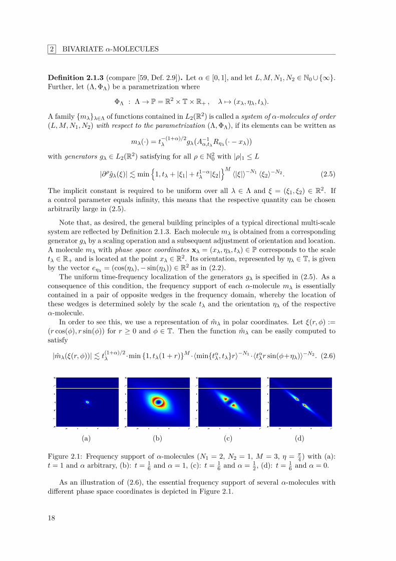
In order to see this, we use a representation of mλ in polar coordinates. Let ξ(r, φ) :=(r cos(φ), r sin(φ)) for r ≥ 0 and φ ∈ T. Then the function mλ can be easily computed tosatisfy
|mλ(ξ(r, φ))| . t(1+α)/2λ ·min 1, tλ(1 + r)M ·⟨mintαλ , tλr⟩−N1 ·⟨tαλr sin(φ+ηλ)⟩−N2 . (2.6)
(a) (b) (c) (d)
Figure 2.1: Frequency support of α-molecules (N1 = 2, N2 = 1, M = 3, η = π4 ) with (a):
t = 1 and α arbitrary, (b): t = 16 and α = 1, (c): t = 1
6 and α = 12 , (d): t = 1
6 and α = 0.
As an illustration of (2.6), the essential frequency support of several α-molecules withdifferent phase space coordinates is depicted in Figure 2.1.
18
2.2 Metrization of the Parameter Space
On the spatial side, the essential support of mλ can be thought of as being contained inthe rectangle xλ +R−1
ηλAα,tλ
Q of dimensions tλ × tαλ , where Q := [−1, 1]2.Finally, we remark that the normalization factor occurring in the α-molecule definition
ensures the equality ∥mλ|L2∥ = ∥gλ|L2∥ for all λ ∈ Λ. In combination with condition (2.5),we can deduce that an α-molecule system of order (L,M,N1, N2) is L2-bounded under themild assumption N1 > 1.Lemma 2.1.4. Let Mα = mλλ∈Λ be a system of α-molecules of order (L,M,N1, N2)with respect to some arbitrary parametrization (Λ,ΦΛ). If N1 > 1 its elements satisfy
supλ∈Λ
∥mλ|L2∥ < ∞.
Proof. Let N1 > 1. Then we have uniformly for all λ ∈ Λ
∥mλ|L2∥2 = ∥gλ|L2∥2 = ∥gλ|L2∥2 .R2
(1 + |ξ|2)−N1 dξ < ∞.
Finally, with a viable notion of α-molecules at hand, we could verify the unifying qualitiesof this notion by providing some concrete examples. However, we postpone this investigationto Chapter 3 and instead proceed with the development of the general theory.
2.2 Metrization of the Parameter Space
Our next goal is to develop appropriate tools enabling the analysis of α-molecule systems ona generic level. For instance, one might be interested in frame or approximation propertiesof such systems, which we will in fact investigate later in Sections 2.3 and 2.4. Also theproperties of associated transforms might be of interest, which will be relevant for us inChapter 4.
A fundamental tool for the analysis of function systems in general is given by the so-called cross-Gramian matrices G[M,M] associated to any two systems M := mλλ∈Λ andM := mµµ∈∆ in L2(R2). Their entries are the scalar products ⟨mλ, mµ⟩, also called thecross-correlations, of the individual functions from M and M. Depending on the index setsΛ and ∆, the cross-Gramian G[M,M] is thus the possibly infinite-dimensional matrix
G[M,M] :=⟨mλ, mµ⟩
λ∈Λ,µ∈∆. (2.7)
In case of a single system, i.e., when M = M, the notation is simplified G[M] := G[M,M]and we call the matrix G[M] just the Gramian matrix of the system M.
The cross-Gramian matrix (2.7) of two function systems contains essential informationabout the mutual relationship of the system elements. A careful analysis enables a compar-ison of the different systems and can also reveal many inherent properties of the systemsthemselves. In particular, cross-Gramians play a pivotal role in frame theory and coorbittheory for example.
Turning our attention to systems Mα and Mα of α-molecules, a fundamental result willbe the fact that the associated cross-Gramian G[Mα,Mα] can be bounded based solely on theorder and the parametrization of the respective systems. This is shown in Theorem 2.2.2, themain result of the next subsection. Moreover, it is possible to define a distance function ωα :P×P → [1,∞) such that for α-molecules mλ ∈ M and mµ ∈ M a higher distance ωα(xλ,xµ)of their respective phase-space coordinates corresponds to a lower cross-correlation.
19
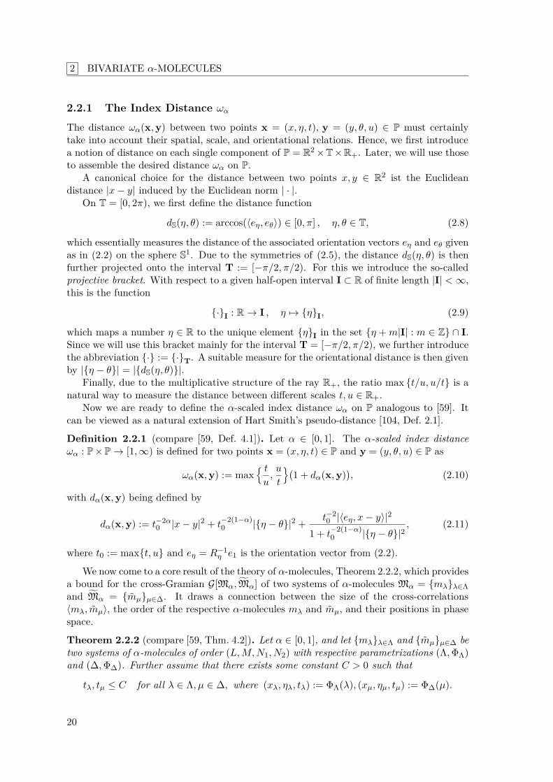
2 BIVARIATE α-MOLECULES
2.2.1 The Index Distance ωα
The distance ωα(x,y) between two points x = (x, η, t), y = (y, θ, u) ∈ P must certainlytake into account their spatial, scale, and orientational relations. Hence, we first introducea notion of distance on each single component of P = R2 ×T×R+. Later, we will use thoseto assemble the desired distance ωα on P.
A canonical choice for the distance between two points x, y ∈ R2 ist the Euclideandistance |x− y| induced by the Euclidean norm | · |.
On T = [0, 2π), we first define the distance function
dS(η, θ) := arccos(⟨eη, eθ⟩) ∈ [0, π] , η, θ ∈ T, (2.8)
which essentially measures the distance of the associated orientation vectors eη and eθ givenas in (2.2) on the sphere S1. Due to the symmetries of (2.5), the distance dS(η, θ) is thenfurther projected onto the interval T := [−π/2, π/2). For this we introduce the so-calledprojective bracket. With respect to a given half-open interval I ⊂ R of finite length |I| < ∞,this is the function
·I : R → I , η →→ ηI, (2.9)
which maps a number η ∈ R to the unique element ηI in the set η +m|I| : m ∈ Z ∩ I.Since we will use this bracket mainly for the interval T = [−π/2, π/2), we further introducethe abbreviation · := ·T. A suitable measure for the orientational distance is then givenby |η − θ| = |dS(η, θ)|.
Finally, due to the multiplicative structure of the ray R+, the ratio max t/u, u/t is anatural way to measure the distance between different scales t, u ∈ R+.
Now we are ready to define the α-scaled index distance ωα on P analogous to [59]. Itcan be viewed as a natural extension of Hart Smith’s pseudo-distance [104, Def. 2.1].
Definition 2.2.1 (compare [59, Def. 4.1]). Let α ∈ [0, 1]. The α-scaled index distanceωα : P×P → [1,∞) is defined for two points x = (x, η, t) ∈ P and y = (y, θ, u) ∈ P as
ωα(x,y) := max tu,u
t
1 + dα(x,y)
, (2.10)
with dα(x,y) being defined by
dα(x,y) := t−2α0 |x− y|2 + t
−2(1−α)0 |η − θ|2 + t−2
0 |⟨eη, x− y⟩|2
1 + t−2(1−α)0 |η − θ|2
, (2.11)
where t0 := maxt, u and eη = R−1η e1 is the orientation vector from (2.2).
We now come to a core result of the theory of α-molecules, Theorem 2.2.2, which providesa bound for the cross-Gramian G[Mα,Mα] of two systems of α-molecules Mα = mλλ∈Λand Mα = mµµ∈∆. It draws a connection between the size of the cross-correlations⟨mλ, mµ⟩, the order of the respective α-molecules mλ and mµ, and their positions in phasespace.
Theorem 2.2.2 (compare [59, Thm. 4.2]). Let α ∈ [0, 1], and let mλλ∈Λ and mµµ∈∆ betwo systems of α-molecules of order (L,M,N1, N2) with respective parametrizations (Λ,ΦΛ)and (∆,Φ∆). Further assume that there exists some constant C > 0 such that
tλ, tµ ≤ C for all λ ∈ Λ, µ ∈ ∆, where (xλ, ηλ, tλ) := ΦΛ(λ), (xµ, ηµ, tµ) := Φ∆(µ).
20
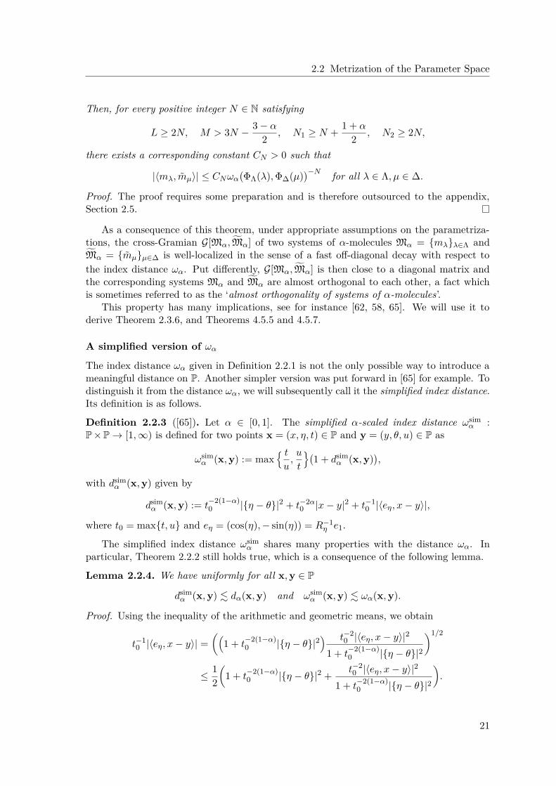
2.2 Metrization of the Parameter Space
Then, for every positive integer N ∈ N satisfying
L ≥ 2N, M > 3N − 3 − α
2 , N1 ≥ N + 1 + α
2 , N2 ≥ 2N,
there exists a corresponding constant CN > 0 such that
|⟨mλ, mµ⟩| ≤ CNωαΦΛ(λ),Φ∆(µ)
−N for all λ ∈ Λ, µ ∈ ∆.
Proof. The proof requires some preparation and is therefore outsourced to the appendix,Section 2.5.
As a consequence of this theorem, under appropriate assumptions on the parametriza-tions, the cross-Gramian G[Mα,Mα] of two systems of α-molecules Mα = mλλ∈Λ andMα = mµµ∈∆ is well-localized in the sense of a fast off-diagonal decay with respect tothe index distance ωα. Put differently, G[Mα,Mα] is then close to a diagonal matrix andthe corresponding systems Mα and Mα are almost orthogonal to each other, a fact whichis sometimes referred to as the ‘almost orthogonality of systems of α-molecules’.
This property has many implications, see for instance [62, 58, 65]. We will use it toderive Theorem 2.3.6, and Theorems 4.5.5 and 4.5.7.
A simplified version of ωα
The index distance ωα given in Definition 2.2.1 is not the only possible way to introduce ameaningful distance on P. Another simpler version was put forward in [65] for example. Todistinguish it from the distance ωα, we will subsequently call it the simplified index distance.Its definition is as follows.
Definition 2.2.3 ([65]). Let α ∈ [0, 1]. The simplified α-scaled index distance ωsimα :
P×P → [1,∞) is defined for two points x = (x, η, t) ∈ P and y = (y, θ, u) ∈ P as
ωsimα (x,y) := max
tu,u
t
1 + dsim
α (x,y),
with dsimα (x,y) given by
dsimα (x,y) := t
−2(1−α)0 |η − θ|2 + t−2α
0 |x− y|2 + t−10 |⟨eη, x− y⟩|,
where t0 = maxt, u and eη = (cos(η),− sin(η)) = R−1η e1.
The simplified index distance ωsimα shares many properties with the distance ωα. In
particular, Theorem 2.2.2 still holds true, which is a consequence of the following lemma.
Lemma 2.2.4. We have uniformly for all x,y ∈ P
dsimα (x,y) . dα(x,y) and ωsim
α (x,y) . ωα(x,y).
Proof. Using the inequality of the arithmetic and geometric means, we obtain
t−10 |⟨eη, x− y⟩| =
1 + t
−2(1−α)0 |η − θ|2
t−20 |⟨eη, x− y⟩|2
1 + t−2(1−α)0 |η − θ|2
1/2
≤ 12
1 + t
−2(1−α)0 |η − θ|2 + t−2
0 |⟨eη, x− y⟩|2
1 + t−2(1−α)0 |η − θ|2
.
21
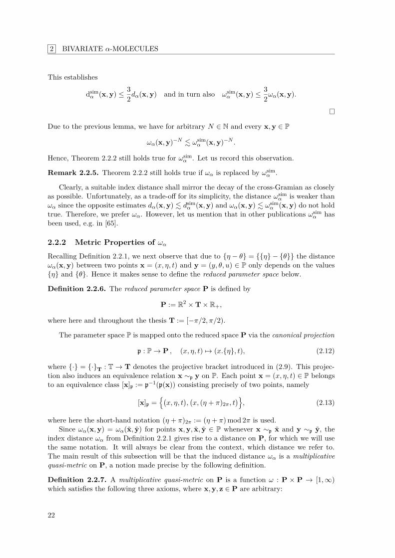
2 BIVARIATE α-MOLECULES
This establishes
dsimα (x,y) ≤ 3
2dα(x,y) and in turn also ωsimα (x,y) ≤ 3
2ωα(x,y).
Due to the previous lemma, we have for arbitrary N ∈ N and every x,y ∈ P
ωα(x,y)−N . ωsimα (x,y)−N .
Hence, Theorem 2.2.2 still holds true for ωsimα . Let us record this observation.
Remark 2.2.5. Theorem 2.2.2 still holds true if ωα is replaced by ωsimα .
Clearly, a suitable index distance shall mirror the decay of the cross-Gramian as closelyas possible. Unfortunately, as a trade-off for its simplicity, the distance ωsim
α is weaker thanωα since the opposite estimates dα(x,y) . dsim
α (x,y) and ωα(x,y) . ωsimα (x,y) do not hold
true. Therefore, we prefer ωα. However, let us mention that in other publications ωsimα has
been used, e.g. in [65].
2.2.2 Metric Properties of ωα
Recalling Definition 2.2.1, we next observe that due to η − θ = η − θ the distanceωα(x,y) between two points x = (x, η, t) and y = (y, θ, u) ∈ P only depends on the valuesη and θ. Hence it makes sense to define the reduced parameter space below.
Definition 2.2.6. The reduced parameter space P is defined by
P := R2 × T × R+,
where here and throughout the thesis T := [−π/2, π/2).
The parameter space P is mapped onto the reduced space P via the canonical projection
p : P → P , (x, η, t) →→ (x.η, t), (2.12)
where · = ·T : T → T denotes the projective bracket introduced in (2.9). This projec-tion also induces an equivalence relation x ∼p y on P. Each point x = (x, η, t) ∈ P belongsto an equivalence class [x]p := p−1(p(x)) consisting precisely of two points, namely
[x]p =x, η, t
,x, (η + π)2π, t
, (2.13)
where here the short-hand notation (η + π)2π := (η + π) mod 2π is used.Since ωα(x,y) = ωα(x, y) for points x,y, x, y ∈ P whenever x ∼p x and y ∼p y, the
index distance ωα from Definition 2.2.1 gives rise to a distance on P, for which we will usethe same notation. It will always be clear from the context, which distance we refer to.The main result of this subsection will be that the induced distance ωα is a multiplicativequasi-metric on P, a notion made precise by the following definition.
Definition 2.2.7. A multiplicative quasi-metric on P is a function ω : P × P → [1,∞)which satisfies the following three axioms, where x,y, z ∈ P are arbitrary:
22
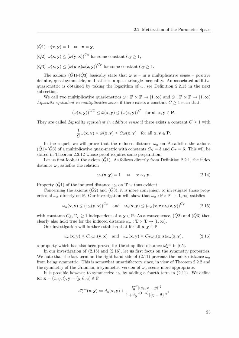
2.2 Metrization of the Parameter Space
(Q1) ω(x,y) = 1 ⇔ x = y,
(Q2) ω(x,y) ≤ω(y,x)
CS for some constant CS ≥ 1,
(Q3) ω(x,y) ≤ω(x, z)ω(z,y)
CT for some constant CT ≥ 1.
The axioms (Q1)-(Q3) basically state that ω is – in a multiplicative sense – positivedefinite, quasi-symmetric, and satisfies a quasi-triangle inequality. An associated additivequasi-metric is obtained by taking the logarithm of ω, see Definition 2.2.13 in the nextsubsection.
We call two multiplicative quasi-metrics ω : P × P → [1,∞) and ω : P × P → [1,∞)Lipschitz equivalent in multiplicative sense if there exists a constant C ≥ 1 such that
ω(x,y)1/C ≤ ω(x,y) ≤
ω(x,y)
C for all x,y ∈ P.
They are called Lipschitz equivalent in additive sense if there exists a constant C ≥ 1 with
1Cω(x,y) ≤ ω(x,y) ≤ Cω(x,y) for all x,y ∈ P.
In the sequel, we will prove that the reduced distance ωα on P satisfies the axioms(Q1)-(Q3) of a multiplicative quasi-metric with constants CS = 3 and CT = 6. This will bestated in Theorem 2.2.12 whose proof requires some preparation.
Let us first look at the axiom (Q1). As follows directly from Definition 2.2.1, the indexdistance ωα satisfies the relation
ωα(x,y) = 1 ⇔ x ∼p y. (2.14)
Property (Q1) of the induced distance ωα on T is thus evident.Concerning the axioms (Q2) and (Q3), it is more convenient to investigate those prop-
erties of ωα directly on P. Our investigation will show that ωα : P×P → [1,∞) satisfies
ωα(x,y) ≤ωα(y,x)
CS and ωα(x,y) ≤ωα(x, z)ωα(z,y)
CT (2.15)
with constants CS , CT ≥ 1 independent of x,y ∈ P. As a consequence, (Q2) and (Q3) thenclearly also hold true for the induced distance ωα : T × T → [1,∞).
Our investigation will further establish that for all x,y ∈ P
ωα(x,y) ≤ CSωα(y,x) and ωα(x,y) ≤ CTωα(x, z)ωα(z,y), (2.16)
a property which has also been proved for the simplified distance ωsimα in [65].
In our investigation of (2.15) and (2.16), let us first focus on the symmetry properties.We note that the last term on the right-hand side of (2.11) prevents the index distance ωα
from being symmetric. This is somewhat unsatisfactory since, in view of Theorem 2.2.2 andthe symmetry of the Gramian, a symmetric version of ωα seems more appropriate.
It is possible however to symmetrize ωα by adding a fourth term in (2.11). We definefor x = (x, η, t),y = (y, θ, u) ∈ P
dsymα (x,y) := dα(x,y) + t−2
0 |⟨eθ, x− y⟩|2
1 + t−2(1−α)0 |η − θ|2
,
23
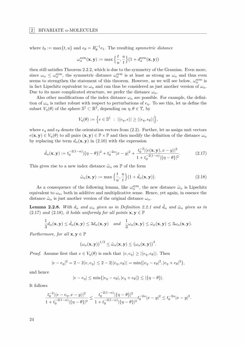
2 BIVARIATE α-MOLECULES
where t0 := maxt, u and eθ = R−1θ e1. The resulting symmetric distance
ωsymα (x,y) := max
tu,u
t
1 + dsym
α (x,y)
then still satisfies Theorem 2.2.2, which is due to the symmetry of the Gramian. Even more,since ωα ≤ ωsym
α , the symmetric distance ωsymα is at least as strong as ωα and thus even
seems to strengthen the statement of this theorem. However, as we will see below, ωsymα is
in fact Lipschitz equivalent to ωα and can thus be considered as just another version of ωα.Due to its more complicated structure, we prefer the distance ωα.
Also other modifications of the index distance ωα are possible. For example, the defini-tion of ωα is rather robust with respect to perturbations of eη. To see this, let us define thesubset Vη(θ) of the sphere S1 ⊂ R2, depending on η, θ ∈ T, by
Vη(θ) :=e ∈ S1 : |⟨eη, e⟩| ≥ |⟨eη, eθ⟩|
,
where eη and eθ denote the orientation vectors from (2.2). Further, let us assign unit vectorse(x,y) ∈ Vη(θ) to all pairs (x,y) ∈ P×P and then modify the definition of the distance ωα
by replacing the term dα(x,y) in (2.10) with the expression
dα(x,y) := t−2(1−α)0 |η − θ|2 + t−2α
0 |x− y|2 + t−20 |⟨e(x,y), x− y⟩|2
1 + t−2(1−α)0 |η − θ|2
. (2.17)
This gives rise to a new index distance ωα on P of the form
ωα(x,y) := max tu,u
t
1 + dα(x,y)
. (2.18)
As a consequence of the following lemma, like ωsymα , the new distance ωα is Lipschitz
equivalent to ωα, both in additive and multiplicative sense. Hence, yet again, in essence thedistance ωα is just another version of the original distance ωα.
Lemma 2.2.8. With dα and ωα given as in Definition 2.2.1 and dα and ωα given as in(2.17) and (2.18), it holds uniformly for all points x,y ∈ P
13dα(x,y) ≤ dα(x,y) ≤ 3dα(x,y) and 1
3ωα(x,y) ≤ ωα(x,y) ≤ 3ωα(x,y).
Furthermore, for all x,y ∈ Pωα(x,y)
1/3 ≤ ωα(x,y) ≤ωα(x,y)
3.
Proof. Assume first that e ∈ Vη(θ) is such that ⟨e, eη⟩ ≥ |⟨eη, eθ⟩|. Then
|e− eη|2 = 2 − 2⟨e, eη⟩ ≤ 2 − 2|⟨eη, eθ⟩| = min|eη − eθ|2, |eη + eθ|2,
and hence|e− eη| ≤ min|eη − eθ|, |eη + eθ| ≤ |η − θ|.
It follows
t−20 |⟨e− eη, x− y⟩|2
1 + t−2(1−α)0 |η − θ|2
≤ t−2(1−α)0 |η − θ|2
1 + t−2(1−α)0 |η − θ|2
t−2α0 |x− y|2 ≤ t−2α
0 |x− y|2.
24
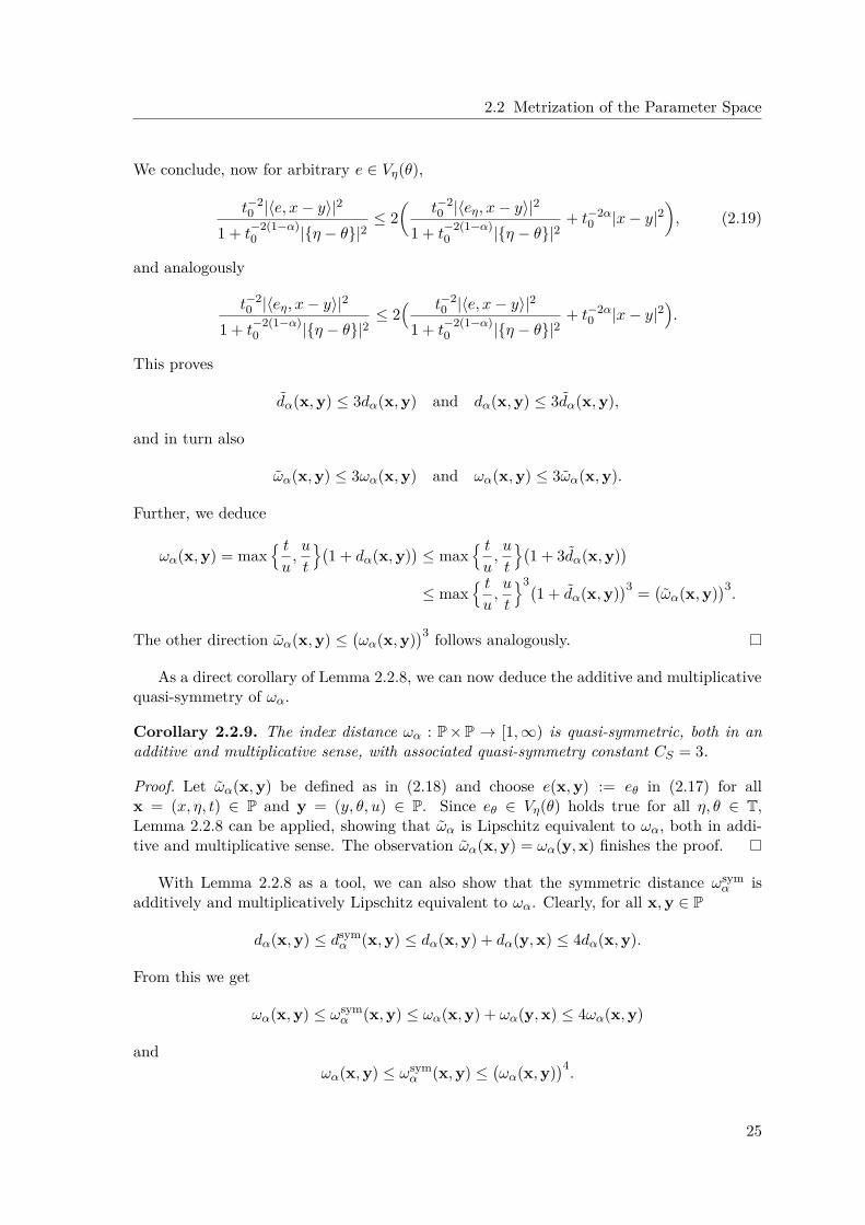
2.2 Metrization of the Parameter Space
We conclude, now for arbitrary e ∈ Vη(θ),
t−20 |⟨e, x− y⟩|2
1 + t−2(1−α)0 |η − θ|2
≤ 2
t−20 |⟨eη, x− y⟩|2
1 + t−2(1−α)0 |η − θ|2
+ t−2α0 |x− y|2
, (2.19)
and analogously
t−20 |⟨eη, x− y⟩|2
1 + t−2(1−α)0 |η − θ|2
≤ 2 t−2
0 |⟨e, x− y⟩|2
1 + t−2(1−α)0 |η − θ|2
+ t−2α0 |x− y|2
.
This proves
dα(x,y) ≤ 3dα(x,y) and dα(x,y) ≤ 3dα(x,y),
and in turn also
ωα(x,y) ≤ 3ωα(x,y) and ωα(x,y) ≤ 3ωα(x,y).
Further, we deduce
ωα(x,y) = max tu,u
t
1 + dα(x,y)
≤ max
tu,u
t
1 + 3dα(x,y)
≤ max
tu,u
t
31 + dα(x,y)
3 =ωα(x,y)
3.
The other direction ωα(x,y) ≤ωα(x,y)
3 follows analogously.
As a direct corollary of Lemma 2.2.8, we can now deduce the additive and multiplicativequasi-symmetry of ωα.
Corollary 2.2.9. The index distance ωα : P×P → [1,∞) is quasi-symmetric, both in anadditive and multiplicative sense, with associated quasi-symmetry constant CS = 3.
Proof. Let ωα(x,y) be defined as in (2.18) and choose e(x,y) := eθ in (2.17) for allx = (x, η, t) ∈ P and y = (y, θ, u) ∈ P. Since eθ ∈ Vη(θ) holds true for all η, θ ∈ T,Lemma 2.2.8 can be applied, showing that ωα is Lipschitz equivalent to ωα, both in addi-tive and multiplicative sense. The observation ωα(x,y) = ωα(y,x) finishes the proof.
With Lemma 2.2.8 as a tool, we can also show that the symmetric distance ωsymα is
additively and multiplicatively Lipschitz equivalent to ωα. Clearly, for all x,y ∈ P
dα(x,y) ≤ dsymα (x,y) ≤ dα(x,y) + dα(y,x) ≤ 4dα(x,y).
From this we get
ωα(x,y) ≤ ωsymα (x,y) ≤ ωα(x,y) + ωα(y,x) ≤ 4ωα(x,y)
andωα(x,y) ≤ ωsym
α (x,y) ≤ωα(x,y)
4.
25
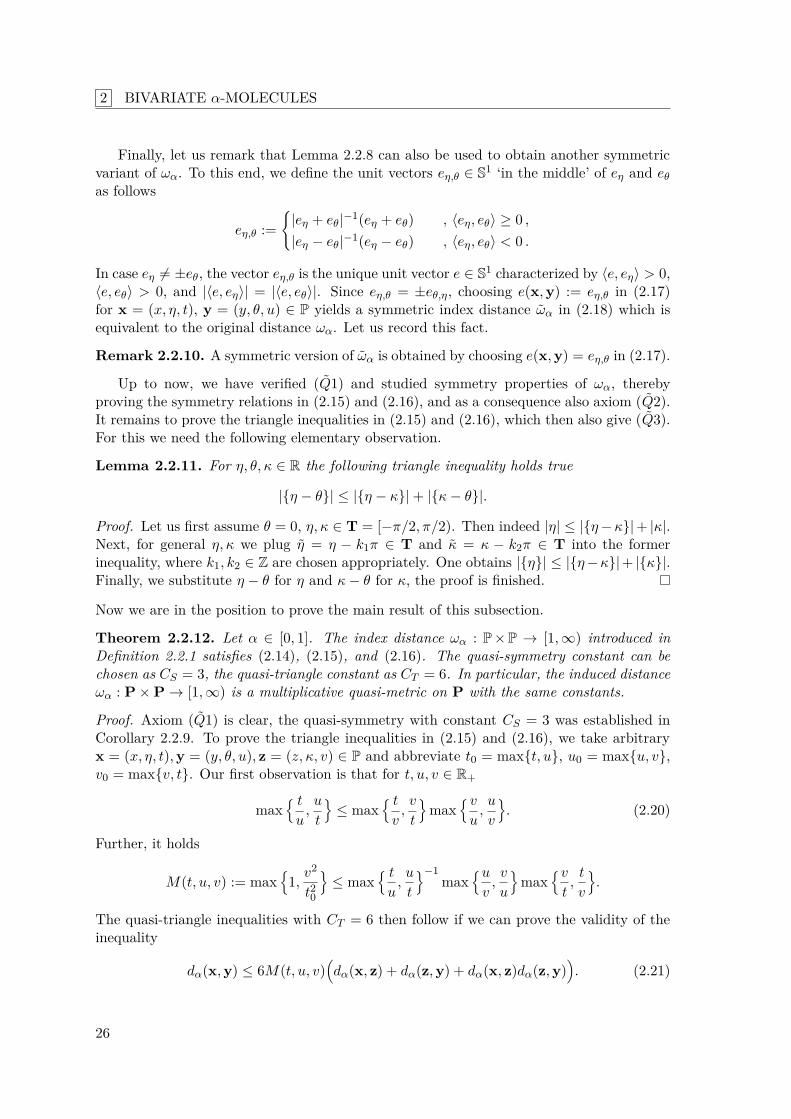
2 BIVARIATE α-MOLECULES
Finally, let us remark that Lemma 2.2.8 can also be used to obtain another symmetricvariant of ωα. To this end, we define the unit vectors eη,θ ∈ S1 ‘in the middle’ of eη and eθ
as follows
eη,θ :=
|eη + eθ|−1(eη + eθ) , ⟨eη, eθ⟩ ≥ 0 ,|eη − eθ|−1(eη − eθ) , ⟨eη, eθ⟩ < 0 .
In case eη = ±eθ, the vector eη,θ is the unique unit vector e ∈ S1 characterized by ⟨e, eη⟩ > 0,⟨e, eθ⟩ > 0, and |⟨e, eη⟩| = |⟨e, eθ⟩|. Since eη,θ = ±eθ,η, choosing e(x,y) := eη,θ in (2.17)for x = (x, η, t), y = (y, θ, u) ∈ P yields a symmetric index distance ωα in (2.18) which isequivalent to the original distance ωα. Let us record this fact.
Remark 2.2.10. A symmetric version of ωα is obtained by choosing e(x,y) = eη,θ in (2.17).
Up to now, we have verified (Q1) and studied symmetry properties of ωα, therebyproving the symmetry relations in (2.15) and (2.16), and as a consequence also axiom (Q2).It remains to prove the triangle inequalities in (2.15) and (2.16), which then also give (Q3).For this we need the following elementary observation.
Lemma 2.2.11. For η, θ, κ ∈ R the following triangle inequality holds true
|η − θ| ≤ |η − κ| + |κ− θ|.
Proof. Let us first assume θ = 0, η, κ ∈ T = [−π/2, π/2). Then indeed |η| ≤ |η−κ| + |κ|.Next, for general η, κ we plug η = η − k1π ∈ T and κ = κ − k2π ∈ T into the formerinequality, where k1, k2 ∈ Z are chosen appropriately. One obtains |η| ≤ |η−κ| + |κ|.Finally, we substitute η − θ for η and κ− θ for κ, the proof is finished.
Now we are in the position to prove the main result of this subsection.
Theorem 2.2.12. Let α ∈ [0, 1]. The index distance ωα : P×P → [1,∞) introduced inDefinition 2.2.1 satisfies (2.14), (2.15), and (2.16). The quasi-symmetry constant can bechosen as CS = 3, the quasi-triangle constant as CT = 6. In particular, the induced distanceωα : P × P → [1,∞) is a multiplicative quasi-metric on P with the same constants.
Proof. Axiom (Q1) is clear, the quasi-symmetry with constant CS = 3 was established inCorollary 2.2.9. To prove the triangle inequalities in (2.15) and (2.16), we take arbitraryx = (x, η, t),y = (y, θ, u), z = (z, κ, v) ∈ P and abbreviate t0 = maxt, u, u0 = maxu, v,v0 = maxv, t. Our first observation is that for t, u, v ∈ R+
max tu,u
t
≤ max
tv,v
t
max
vu,u
v
. (2.20)
Further, it holds
M(t, u, v) := max
1, v2
t20
≤ max
tu,u
t
−1max
uv,v
u
max
vt,t
v
.
The quasi-triangle inequalities with CT = 6 then follow if we can prove the validity of theinequality
dα(x,y) ≤ 6M(t, u, v)dα(x, z) + dα(z,y) + dα(x, z)dα(z,y)
. (2.21)
26
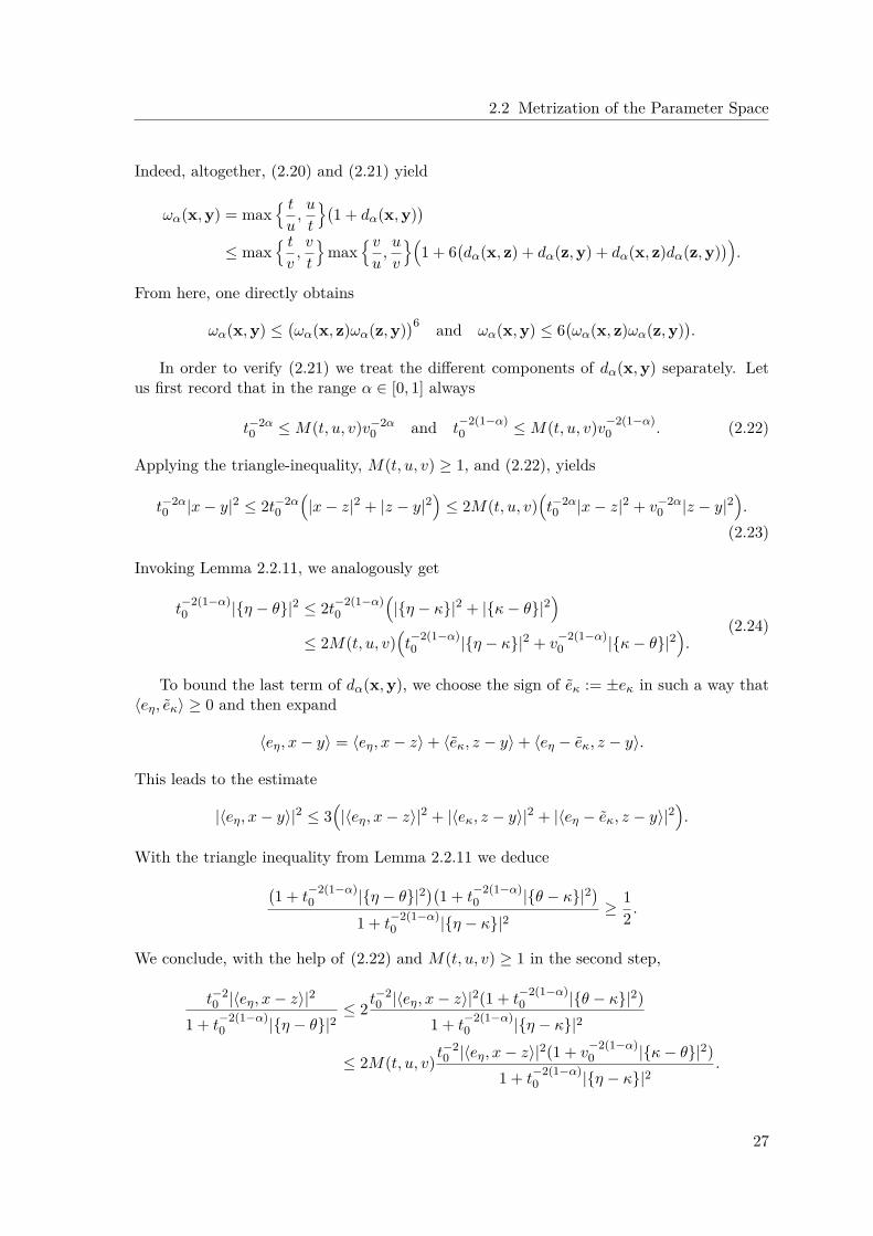
2.2 Metrization of the Parameter Space
Indeed, altogether, (2.20) and (2.21) yield
ωα(x,y) = max tu,u
t
1 + dα(x,y)
≤ max
tv,v
t
max
vu,u
v
1 + 6
dα(x, z) + dα(z,y) + dα(x, z)dα(z,y)
.
From here, one directly obtains
ωα(x,y) ≤ωα(x, z)ωα(z,y)
6 and ωα(x,y) ≤ 6ωα(x, z)ωα(z,y)
.
In order to verify (2.21) we treat the different components of dα(x,y) separately. Letus first record that in the range α ∈ [0, 1] always
t−2α0 ≤ M(t, u, v)v−2α
0 and t−2(1−α)0 ≤ M(t, u, v)v−2(1−α)
0 . (2.22)
Applying the triangle-inequality, M(t, u, v) ≥ 1, and (2.22), yields
t−2α0 |x− y|2 ≤ 2t−2α
0
|x− z|2 + |z − y|2
≤ 2M(t, u, v)
t−2α0 |x− z|2 + v−2α
0 |z − y|2.
(2.23)
Invoking Lemma 2.2.11, we analogously get
t−2(1−α)0 |η − θ|2 ≤ 2t−2(1−α)
0
|η − κ|2 + |κ− θ|2
≤ 2M(t, u, v)
t−2(1−α)0 |η − κ|2 + v
−2(1−α)0 |κ− θ|2
.
(2.24)
To bound the last term of dα(x,y), we choose the sign of eκ := ±eκ in such a way that⟨eη, eκ⟩ ≥ 0 and then expand
⟨eη, x− y⟩ = ⟨eη, x− z⟩ + ⟨eκ, z − y⟩ + ⟨eη − eκ, z − y⟩.
This leads to the estimate
|⟨eη, x− y⟩|2 ≤ 3|⟨eη, x− z⟩|2 + |⟨eκ, z − y⟩|2 + |⟨eη − eκ, z − y⟩|2
.
With the triangle inequality from Lemma 2.2.11 we deduce1 + t
−2(1−α)0 |η − θ|2
1 + t
−2(1−α)0 |θ − κ|2
1 + t
−2(1−α)0 |η − κ|2
≥ 12 .
We conclude, with the help of (2.22) and M(t, u, v) ≥ 1 in the second step,
t−20 |⟨eη, x− z⟩|2
1 + t−2(1−α)0 |η − θ|2
≤ 2 t−20 |⟨eη, x− z⟩|2(1 + t
−2(1−α)0 |θ − κ|2)
1 + t−2(1−α)0 |η − κ|2
≤ 2M(t, u, v) t−20 |⟨eη, x− z⟩|2(1 + v
−2(1−α)0 |κ− θ|2)
1 + t−2(1−α)0 |η − κ|2
.
27
2 BIVARIATE α-MOLECULES
Similarly, we first verify
t−20 |⟨eκ, z − y⟩|2
1 + t−2(1−α)0 |η − θ|2
≤ 2 t−20 |⟨eκ, z − y⟩|2(1 + t
−2(1−α)0 |κ− η|2)
1 + t−2(1−α)0 |κ− θ|2
.
Assuming v0 ≤ t0 and using M(t, u, v) ≥ 1 in the second step, we then obtain
t−20 |⟨eκ, z − y⟩|2
1 + t−2(1−α)0 |η − θ|2
≤ 2v−20 |⟨eκ, z − y⟩|2(1 + t
−2(1−α)0 |η − κ|2)
1 + v−2(1−α)0 |κ− θ|2
≤ 2M(t, u, v)v−20 |⟨eκ, z − y⟩|2(1 + t
−2(1−α)0 |η − κ|2)
1 + v−2(1−α)0 |κ− θ|2
.
If v0 > t0 we argue differently, using t−20 ≤ M(t, u, v)v−2
0 in the first step,
t−20 |⟨eκ, z − y⟩|2
1 + t−2(1−α)0 |η − θ|2
≤ 2M(t, u, v)v−20 |⟨eκ, z − y⟩|2(1 + t
−2(1−α)0 |η − κ|2)
1 + t−2(1−α)0 |κ− θ|2
≤ 2M(t, u, v)v−20 |⟨eκ, z − y⟩|2(1 + t
−2(1−α)0 |η − κ|2)
1 + v−2(1−α)0 |κ− θ|2
.
Finally, we have
t−20 |⟨eη − eκ, z − y⟩|2
1 + t−2(1−α)0 |η − θ|2
≤ M(t, u, v)t−2(1−α)0 v−2α
0 |η − κ|2|z − y|2,
because of
|⟨eη − eκ, z − y⟩|2 ≤ |eη − eκ|2|z − y|2 ≤ |η − κ|2|z − y|2,
where ⟨eη, eκ⟩ ≥ 0 was used for the last estimate, and the inequality
t−20
1 + t−2(1−α)0 |η − θ|2
≤ t−20 ≤ M(t, u, v)t−2(1−α)
0 v−2α0 ,
where again (2.22) was used in the last step.All in all, we arrive at
t−20 |⟨eη, x− y⟩|2
1 + t−2(1−α)0 |η − θ|2
≤ 6M(t, u, v)t−2(1−α)0 v−2α
0 |η − κ|2|z − y|2+
+ v−20 |⟨eκ, z − y⟩|2t−2(1−α)
0 |η − κ|2
1 + v−2(1−α)0 |κ− θ|2
+ t−20 |⟨eη, x− z⟩|2v−2(1−α)
0 |κ− θ|2
1 + t−2(1−α)0 |η − κ|2
.
This bound together with (2.23) and (2.24) establishes (2.21), and the proof is finished.
In this subsection, we have proved that ωα constitutes a multiplicative quasi-metricon the reduced parameter space P. Further, we have seen that many different equivalentversions of ωα can be defined, even symmetric ones. For the subsequent theory it doesnot matter which version we use, since only the constants would be affected. The reason,why we stick to the original definition of ωα from Definition 2.2.1 is its simpler structurecompared to the other versions.
28
2.2 Metrization of the Parameter Space
2.2.3 α-Balls
We will now discuss in more detail the quasi-metric structure of P induced by ωα. Inparticular, we will investigate the ‘balls’ obtained from ωα. To shift this investigation intomore familiar territory, we first associate to ωα a corresponding additive quasi-metric. Theaxioms of this notion are recalled below.
Definition 2.2.13. An additive quasi-metric on P is a function ω : P × P → [0,∞) whichsatisfies the following three axioms, where x,y, z ∈ P are arbitrary:
(Q1) ω(x,y) = 0 ⇔ x = y,
(Q2) ω(x,y) ≤ CSω(y,x) for some constant CS ≥ 1,
(Q3) ω(x,y) ≤ CT
ω(x, z) + ω(z,y)
for some constant CT ≥ 1.
Since, according to Theorem 2.2.12, ωα constitutes a multiplicative quasi-metric on Psatisfying the axioms (Q1)-(Q3) of Definition 2.2.7, clearly the function
ωlogα (x,y) := log2(ωα(x,y)) = | log2(t/u)| + log2
1 + dα(x,y)
defines an additive quasi-metric on P. We further note that due to (2.15) ωlog
α also fulfillsthe axioms (Q2) and (Q3) as a function on P×P.
The quasi-metric ωlogα gives rise to an associated family of balls in P. The α-balls of
radius τ ≥ 0 are defined by
Bατ (x) :=
y ∈ P : ωlog
α (x,y) ≤ τ
=
y ∈ P : ωα(x,y) ≤ 2τ. (2.25)
Due to the non-symmetry of ωlogα , there also exist the dual α-balls of radius τ ≥ 0 given by
B′,ατ (x) :=
y ∈ P : ωlog
α (y,x) ≤ τ
=
y ∈ P : ωα(y,x) ≤ 2τ.
In general, the dual α-balls B′,ατ (x) do not coincide with the primal α-balls Bα
τ (x). Therelation between the two types of balls is expressed by the equivalence
y ∈ Bατ (x) ⇔ x ∈ B′,α
τ (y).
Subsequently, we will mostly be interested in the primal balls Bατ (x), in particular in a
more explicit representation. Clearly, Bα0 (x) = [x]p for every x ∈ P, where [x]p = p−1p(x)
is the equivalence class (2.13) induced by the canonical projection p : P → P from (2.12).In case of radii τ > 0, let us consider y = (y, θ, u) ∈ Bα
τ (x) at some fixed position x =(x, η, t) ∈ P. We then derive the following necessary conditions from the definition of ωα.
First we see that, due to ωα(x,y) ≤ 2τ and 1 + dα(x,y) ≥ 1, we necessarily have
max tu,u
t
≤ 2τ or equivalently | log2(t/u)| ≤ τ.
Using α ∈ [0, 1] and 1 ≤ maxt/u, u/t ≤ 2τ , we also get
t−2(1−α)|η − θ|2 ≤ 22τ t−2(1−α)0 |η − θ|2 ≤ 22τ (2τ − 1) ≤ 24τ − 1.
29
2 BIVARIATE α-MOLECULES
Further, we deduce
t−2|⟨e1, Rη(x− y)⟩|2 ≤ 22τ t−20 |⟨e1, Rη(x− y)⟩|2 ≤ 23τ (2τ − 1) ≤ 24τ − 1,
where we applied
t−20 |⟨eη, x− y⟩|2 ≤ (2τ − 1)(1 + t
−2(1−α)0 |η − θ|2) ≤ 2τ (2τ − 1).
At last, we bound t−2α|⟨e2, Rη(x− y)⟩|2 by
22τ t−2α0 |⟨e2, Rη(x− y)⟩|2 ≤ 22τ t−2α
0 |x− y|2 ≤ 22τ (2τ − 1) ≤ 24τ − 1.
These estimates motivate the definition of another distance function on P, namely
wα(x,y) := maxt−α|⟨e2, Rη(x− y)⟩|, t−1|⟨e1, Rη(x− y)⟩|, t−(1−α)|η − θ|, | log2(t/u)|
.
Further, we introduce corresponding subsets of P, for x = (x, η, t) ∈ P and τ ≥ 0 the sets
V ατ (x) :=
x+R−1
η Aα,tQτ
×η + t1−αIτ
2π
×tJτ
, (2.26)
where Qτ := [−τ, τ ]2, Iτ := [−τ, τ ], Jτ := [2−τ , 2τ ], and (·)2π := (·)mod 2π, and collectthese in
Vατ := Vα
τ [P] :=V α
τ (x) : x ∈ P.
Then, for every x = (x, η, t) ∈ P and τ ≥ 0 we can write
V ατ
[x]p
:= V α
τ
(x, η, t)
∪ V α
τ
(x, (η + π)2π, t)
=
y ∈ P : wα(x,y) ≤ τ,
where as above [x]p denotes the equivalence class (2.13).We will see below that the sets V α
τ
[x]p
are good approximations of the α-balls Bα
τ (x)as long as the scale parameter remains small. In Chapter 4, where we will only considerthe subspace X = R2 × T × (0, 1] ⊂ P, we can thus use them as convenient substitutes forBα
τ (x), which are easier to handle since they can be expressed explicitly by (2.26).Again, there also exist dual sets which have a slightly more complicated structure. They
are given by
V ′,ατ (x) :=
y ∈ P : x ∈ V α
τ (y)
=
y = (y, θ, u) ∈ P : y ∈ x+R−1θ Aα,uQ
τ , θ ∈η + u1−αIτ
2π, u ∈ tJτ
.
In the following, we will investigate the relation of the sets V ατ ([x]p) to the α-balls Bα
τ (x).As an immediate consequence of the definition of wα, we obtain the lemma below.
Lemma 2.2.14. Let α ∈ [0, 1]. For all x ∈ P and τ ≥ 0
0 ≤ supy∈Bα
τ (x)wα(x,y) ≤
24τ − 1.
30
2.2 Metrization of the Parameter Space
Proof. Let y ∈ Bατ (x) for some fixed x ∈ P and τ ≥ 0. Then, according to the estimates
above,
maxt−α|⟨e2, Rη(x− y)⟩|, t−1|⟨e1, Rη(x− y)⟩|, t−(1−α)|η − θ|
≤
24τ − 1.
Further, it also holds| log2(t/u)| ≤ τ ≤
24τ − 1.
Put differently, Lemma 2.2.14 yields the following inclusion, valid for all x ∈ P andτ ≥ 0,
Bατ (x) ⊆ V α√
24τ −1[x]p
.
To obtain a reverse inclusion, we need the following lemma.
Lemma 2.2.15. Let α ∈ [0, 1]. For all x = (x, η, t) ∈ P and τ ≥ 0
1 ≤ supy∈V α
τ (x)ωα(x,y) ≤ 2τ 1 + 4τ2k(x)2
with a factor k(x) := max1, t1−α which is relevant only if t > 1 and α = 1.
Proof. Let y ∈ V ατ (x) for some fixed x ∈ P and τ ≥ 0. Then we can deduce from (2.26)
that maxt/u, u/t ≤ 2τ and, with dS(η, θ) given as in (2.8),
dS(η, θ) ≤ τt1−α , |⟨e1, Rη(x− y)⟩| ≤ τt , |⟨e2, Rη(x− y)⟩| ≤ τtα.
Since |η − θ| ≤ dS(η, θ) and t0 = maxt, u ≥ t, this implies
t−2(1−α)0 |η − θ|2 ≤ τ2.
Further, we get
t−20 |⟨eη, x− y⟩|2
1 + t−2(1−α)0 |η − θ|2
≤ t−20 |⟨e1, Rη(x− y)⟩|2 ≤ τ2.
Finally, we deduce
|x− y|2 = |⟨e1, Rη(x− y)⟩|2 + |⟨e2, Rη(x− y)⟩|2 ≤ τ2(t2 + t2α).
If t ≤ 1, whence t ≤ tα, this leads to
t−2α0 |x− y|2 ≤ 2t−2α
0 t2ατ2 ≤ 2τ2.
In case t > 1, we have t ≥ tα and obtain
t−2α0 |x− y|2 ≤ 2t−2α
0 t2τ2 ≤ 2τ2t2(1−α).
Altogether, our estimates prove
ωα(x,y) ≤ 2τ (1 + 2τ2 + 2τ2k(x)2) ≤ 2τ (1 + 4τ2k(x)2)
with k(x) = max1, t1−α.
31
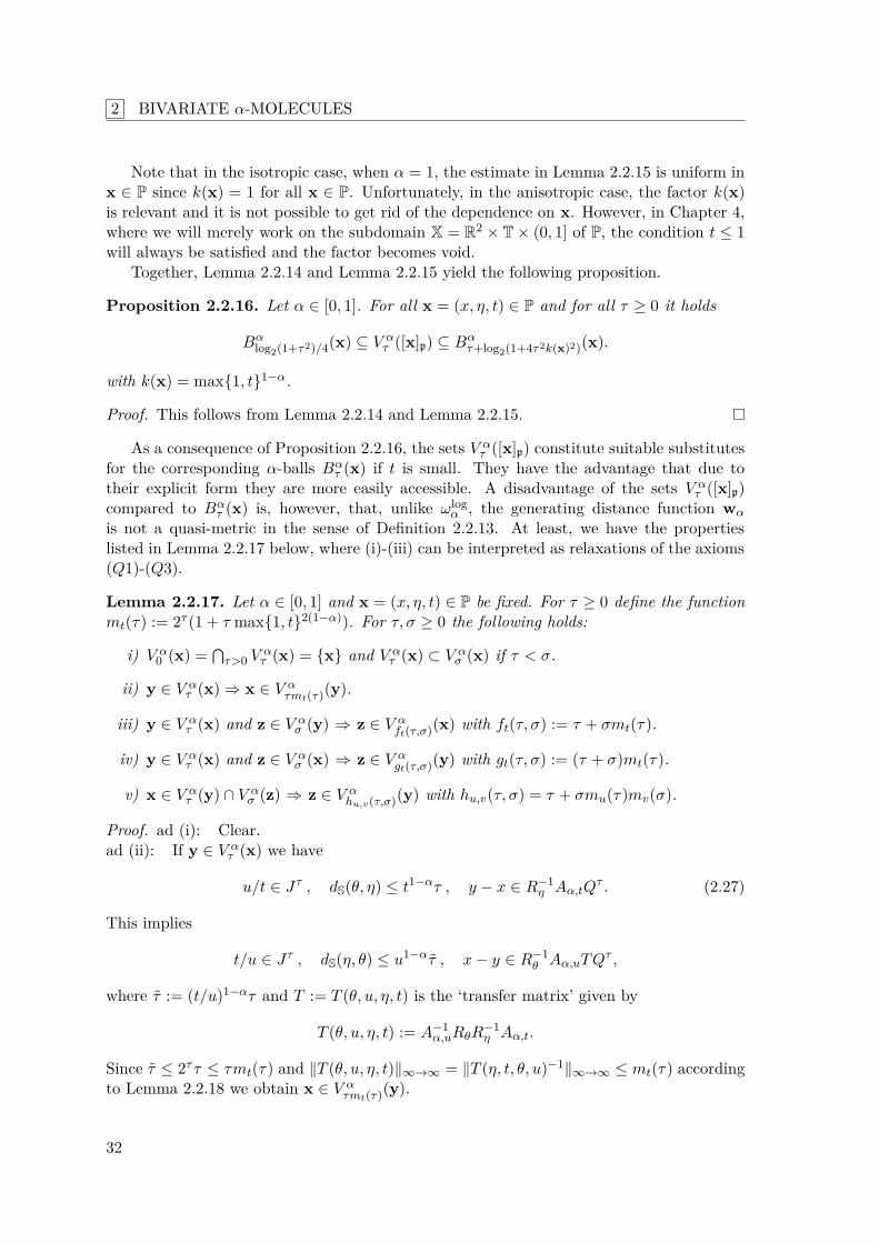
2 BIVARIATE α-MOLECULES
Note that in the isotropic case, when α = 1, the estimate in Lemma 2.2.15 is uniform inx ∈ P since k(x) = 1 for all x ∈ P. Unfortunately, in the anisotropic case, the factor k(x)is relevant and it is not possible to get rid of the dependence on x. However, in Chapter 4,where we will merely work on the subdomain X = R2 × T × (0, 1] of P, the condition t ≤ 1will always be satisfied and the factor becomes void.
Together, Lemma 2.2.14 and Lemma 2.2.15 yield the following proposition.
Proposition 2.2.16. Let α ∈ [0, 1]. For all x = (x, η, t) ∈ P and for all τ ≥ 0 it holds
Bαlog2(1+τ2)/4(x) ⊆ V α
τ ([x]p) ⊆ Bατ+log2(1+4τ2k(x)2)(x).
with k(x) = max1, t1−α.
Proof. This follows from Lemma 2.2.14 and Lemma 2.2.15.
As a consequence of Proposition 2.2.16, the sets V ατ ([x]p) constitute suitable substitutes
for the corresponding α-balls Bατ (x) if t is small. They have the advantage that due to
their explicit form they are more easily accessible. A disadvantage of the sets V ατ ([x]p)
compared to Bατ (x) is, however, that, unlike ωlog
α , the generating distance function wα
is not a quasi-metric in the sense of Definition 2.2.13. At least, we have the propertieslisted in Lemma 2.2.17 below, where (i)-(iii) can be interpreted as relaxations of the axioms(Q1)-(Q3).
Lemma 2.2.17. Let α ∈ [0, 1] and x = (x, η, t) ∈ P be fixed. For τ ≥ 0 define the functionmt(τ) := 2τ (1 + τ max1, t2(1−α)). For τ, σ ≥ 0 the following holds:
i) V α0 (x) =
τ>0 V
ατ (x) = x and V α
τ (x) ⊂ V ασ (x) if τ < σ.
ii) y ∈ V ατ (x) ⇒ x ∈ V α
τmt(τ)(y).
iii) y ∈ V ατ (x) and z ∈ V α
σ (y) ⇒ z ∈ V αft(τ,σ)(x) with ft(τ, σ) := τ + σmt(τ).
iv) y ∈ V ατ (x) and z ∈ V α
σ (x) ⇒ z ∈ V αgt(τ,σ)(y) with gt(τ, σ) := (τ + σ)mt(τ).
v) x ∈ V ατ (y) ∩ V α
σ (z) ⇒ z ∈ V αhu,v(τ,σ)(y) with hu,v(τ, σ) = τ + σmu(τ)mv(σ).
Proof. ad (i): Clear.ad (ii): If y ∈ V α
τ (x) we have
u/t ∈ Jτ , dS(θ, η) ≤ t1−ατ , y − x ∈ R−1η Aα,tQ
τ . (2.27)
This implies
t/u ∈ Jτ , dS(η, θ) ≤ u1−ατ , x− y ∈ R−1θ Aα,uTQ
τ ,
where τ := (t/u)1−ατ and T := T (θ, u, η, t) is the ‘transfer matrix’ given by
T (θ, u, η, t) := A−1α,uRθR
−1η Aα,t.
Since τ ≤ 2ττ ≤ τmt(τ) and ∥T (θ, u, η, t)∥∞→∞ = ∥T (η, t, θ, u)−1∥∞→∞ ≤ mt(τ) accordingto Lemma 2.2.18 we obtain x ∈ V α
τmt(τ)(y).
32
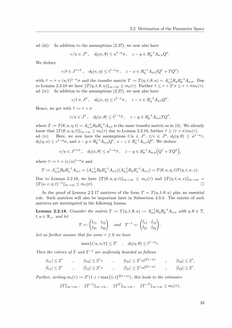
2.2 Metrization of the Parameter Space
ad (iii): In addition to the assumptions (2.27), we now also have
v/u ∈ Jσ , dS(κ, θ) ≤ u1−ασ , z − y ∈ R−1θ Aα,uQ
σ.
We deduce
v/t ∈ Jτ+σ , dS(κ, η) ≤ t1−ατ , z − x ∈ R−1η Aα,t
Qτ + TQσ
with τ = τ + (u/t)1−ασ and the transfer matrix T := T (η, t, θ, u) = A−1α,tRηR
−1θ Aα,u. Due
to Lemma 2.2.18 we have ∥T (η, t, θ, u)∥∞→∞ ≤ mt(τ). Further τ ≤ τ + 2τσ ≤ τ + σmt(τ).ad (iv): In addition to the assumptions (2.27), we now also have
v/t ∈ Jσ , dS(κ, η) ≤ t1−ασ , z − x ∈ R−1η Aα,tQ
σ.
Hence, we get with τ := τ + σ
v/u ∈ J τ , dS(κ, θ) ≤ t1−ατ , z − y ∈ R−1θ Aα,uTQ
τ ,
where T := T (θ, u, η, t) = A−1α,uRθR
−1η Aα,t is the same transfer matrix as in (ii). We already
know that ∥T (θ, u, η, t)∥∞→∞ ≤ mt(τ) due to Lemma 2.2.18, further τ ≤ (τ + σ)mt(τ).ad (v): Here, we now have the assumptions t/u ∈ Jτ , t/v ∈ Jσ, dS(η, θ) ≤ u1−ατ ,dS(η, κ) ≤ v1−ασ, and x− y ∈ R−1
θ Aα,uQτ , x− z ∈ R−1
κ Aα,vQσ. We deduce
v/u ∈ Jτ+σ , dS(κ, θ) ≤ u1−ατ , z − y ∈ R−1θ Aα,u
Qτ + TQσ
,
where τ := τ + (v/u)1−ασ and
T := A−1α,uRθR
−1κ Aα,v =
A−1
α,uRθR−1η Aα,t
A−1
α,tRηR−1κ Aα,v
= T (θ, u, η, t)T (η, t, κ, v).
Due to Lemma 2.2.18, we have ∥T (θ, u, η, t)∥∞→∞ ≤ mu(τ) and ∥T (η, t, κ, v)∥∞→∞ =∥T (κ, v, η, t)−1∥∞→∞ ≤ mv(σ).
In the proof of Lemma 2.2.17 matrices of the form T = T (η, t, θ, u) play an essentialrole. Such matrices will also be important later in Subsection 4.3.4. The entries of suchmatrices are investigated in the following lemma.
Lemma 2.2.18. Consider the matrix T := T (η, t, θ, u) := A−1α,tRηR
−1θ Aα,u with η, θ ∈ T,
t, u ∈ R+, and let
T =:t11 t12t21 t22
and T−1 =:
t11 t12t21 t22
.
Let us further assume that for some τ ≥ 0 we have
maxt/u, u/t ≤ 2τ , dS(η, θ) ≤ t1−ατ.
Then the entries of T and T−1 are uniformly bounded as follows
|t11| ≤ 2τ , |t12| ≤ 2ττ , |t21| ≤ 2ττt2(1−α) , |t22| ≤ 2τ ,
|t11| ≤ 2τ , |t12| ≤ 2ττ , |t21| ≤ 2ττt2(1−α) , |t22| ≤ 2τ .
Further, writing mt(τ) := 2τ (1 + τ max1, t2(1−α)), this leads to the estimates
∥T∥∞→∞ , ∥T−1∥∞→∞ , ∥T T ∥∞→∞ , ∥T−T ∥∞→∞ ≤ mt(τ).
33
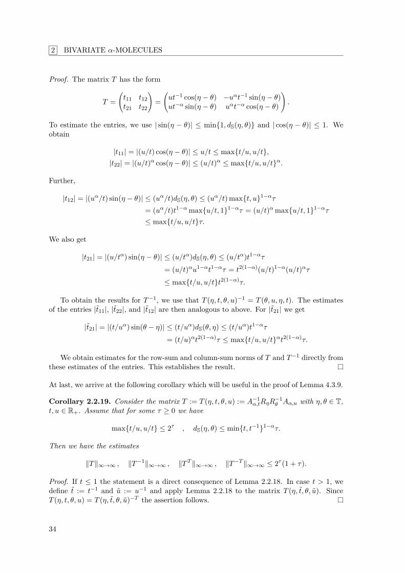
2 BIVARIATE α-MOLECULES
Proof. The matrix T has the form
T =t11 t12t21 t22
=ut−1 cos(η − θ) −uαt−1 sin(η − θ)ut−α sin(η − θ) uαt−α cos(η − θ)
.
To estimate the entries, we use | sin(η − θ)| ≤ min1, dS(η, θ) and | cos(η − θ)| ≤ 1. Weobtain
|t11| = |(u/t) cos(η − θ)| ≤ u/t ≤ maxt/u, u/t,|t22| = |(u/t)α cos(η − θ)| ≤ (u/t)α ≤ maxt/u, u/tα.
Further,
|t12| = |(uα/t) sin(η − θ)| ≤ (uα/t)dS(η, θ) ≤ (uα/t) maxt, u1−ατ
= (uα/t)t1−α maxu/t, 11−ατ = (u/t)α maxu/t, 11−ατ
≤ maxt/u, u/tτ.
We also get
|t21| = |(u/tα) sin(η − θ)| ≤ (u/tα)dS(η, θ) ≤ (u/tα)t1−ατ
= (u/t)αu1−αt1−ατ = t2(1−α)(u/t)1−α(u/t)ατ
≤ maxt/u, u/tt2(1−α)τ.
To obtain the results for T−1, we use that T (η, t, θ, u)−1 = T (θ, u, η, t). The estimatesof the entries |t11|, |t22|, and |t12| are then analogous to above. For |t21| we get
|t21| = |(t/uα) sin(θ − η)| ≤ (t/uα)dS(θ, η) ≤ (t/uα)t1−ατ
= (t/u)αt2(1−α)τ ≤ maxt/u, u/tαt2(1−α)τ.
We obtain estimates for the row-sum and column-sum norms of T and T−1 directly fromthese estimates of the entries. This establishes the result.
At last, we arrive at the following corollary which will be useful in the proof of Lemma 4.3.9.
Corollary 2.2.19. Consider the matrix T := T (η, t, θ, u) := A−1α,tRηR
−1θ Aα,u with η, θ ∈ T,
t, u ∈ R+. Assume that for some τ ≥ 0 we have
maxt/u, u/t ≤ 2τ , dS(η, θ) ≤ mint, t−11−ατ.
Then we have the estimates
∥T∥∞→∞ , ∥T−1∥∞→∞ , ∥T T ∥∞→∞ , ∥T−T ∥∞→∞ ≤ 2τ (1 + τ).
Proof. If t ≤ 1 the statement is a direct consequence of Lemma 2.2.18. In case t > 1, wedefine t := t−1 and u := u−1 and apply Lemma 2.2.18 to the matrix T (η, t, θ, u). SinceT (η, t, θ, u) = T (η, t, θ, u)−T the assertion follows.
34
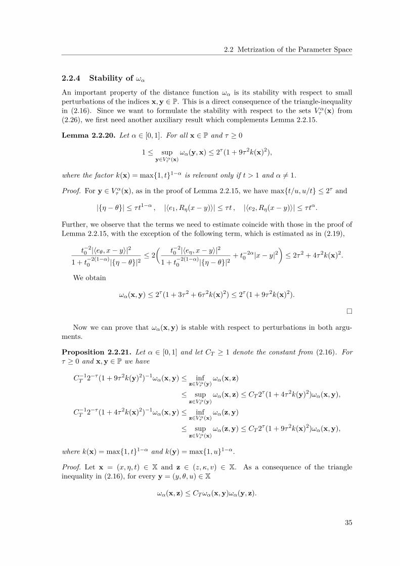
2.2 Metrization of the Parameter Space
2.2.4 Stability of ωα
An important property of the distance function ωα is its stability with respect to smallperturbations of the indices x,y ∈ P. This is a direct consequence of the triangle-inequalityin (2.16). Since we want to formulate the stability with respect to the sets V α
τ (x) from(2.26), we first need another auxiliary result which complements Lemma 2.2.15.
Lemma 2.2.20. Let α ∈ [0, 1]. For all x ∈ P and τ ≥ 0
1 ≤ supy∈V α
τ (x)ωα(y,x) ≤ 2τ (1 + 9τ2k(x)2),
where the factor k(x) = max1, t1−α is relevant only if t > 1 and α = 1.
Proof. For y ∈ V ατ (x), as in the proof of Lemma 2.2.15, we have maxt/u, u/t ≤ 2τ and
|η − θ| ≤ τt1−α , |⟨e1, Rη(x− y)⟩| ≤ τt , |⟨e2, Rη(x− y)⟩| ≤ τtα.
Further, we observe that the terms we need to estimate coincide with those in the proof ofLemma 2.2.15, with the exception of the following term, which is estimated as in (2.19),
t−20 |⟨eθ, x− y⟩|2
1 + t−2(1−α)0 |η − θ|2
≤ 2
t−20 |⟨eη, x− y⟩|2
1 + t−2(1−α)0 |η − θ|2
+ t−2α0 |x− y|2
≤ 2τ2 + 4τ2k(x)2.
We obtain
ωα(x,y) ≤ 2τ (1 + 3τ2 + 6τ2k(x)2) ≤ 2τ (1 + 9τ2k(x)2).
Now we can prove that ωα(x,y) is stable with respect to perturbations in both argu-ments.
Proposition 2.2.21. Let α ∈ [0, 1] and let CT ≥ 1 denote the constant from (2.16). Forτ ≥ 0 and x,y ∈ P we have
C−1T 2−τ (1 + 9τ2k(y)2)−1ωα(x,y) ≤ inf
z∈V ατ (y)
ωα(x, z)
≤ supz∈V α
τ (y)ωα(x, z) ≤ CT 2τ (1 + 4τ2k(y)2)ωα(x,y),
C−1T 2−τ (1 + 4τ2k(x)2)−1ωα(x,y) ≤ inf
z∈V ατ (x)
ωα(z,y)
≤ supz∈V α
τ (x)ωα(z,y) ≤ CT 2τ (1 + 9τ2k(x)2)ωα(x,y),
where k(x) = max1, t1−α and k(y) = max1, u1−α.
Proof. Let x = (x, η, t) ∈ X and z ∈ (z, κ, v) ∈ X. As a consequence of the triangleinequality in (2.16), for every y = (y, θ, u) ∈ X
ωα(x, z) ≤ CTωα(x,y)ωα(y, z).
35
2 BIVARIATE α-MOLECULES
Together with Lemma 2.2.15, this yields
supz∈V α
τ (y)ωα(x, z) ≤ CTωα(x,y) sup
z∈V ατ (y)
ωα(y, z) ≤ CT 2τ (1 + 4τ2k(y)2)ωα(x,y).
The triangle inequality also yields ωα(x,y) ≤ CTωα(x, z)ωα(z,y) which implies
C−1T ωα(z,y)−1ωα(x,y) ≤ ωα(x, z).
We deduce with Lemma 2.2.20
infz∈V α
τ (y)ωα(x, z) ≥ C−1
T infz∈V α
τ (y)
ωα(z,y)−1ωα(x,y)
= C−1T
sup
z∈V ατ (y)
ωα(z,y)−1
ωα(x,y) ≥ C−1T 2−τ (1 + 9τ2k(y)2)−1ωα(x,y).
Similarly, the second inequality is shown.
We can draw the following conclusion, which will be relevant in Chapter 4.
Corollary 2.2.22. Let C > 0 and τ ≥ 0 be fixed. Then we have
supa∈V α
τ (x)sup
b∈V ατ (y)
ωα(a,b) . ωα(x,y) . infa∈V α
τ (x)inf
b∈V ατ (y)
ωα(a,b)
uniformly for all x = (x, η, t) ∈ P and y = (y, θ, u) ∈ P with t, u ≤ C.
2.3 Transfer Principle for Discrete α-Molecule Frames
In this section, we take a first step towards the analysis of approximation properties of α-molecule systems. Our main result, Theorem 2.3.6 ([59, Thm. 5.6]), will lay the foundationfor a systematic comparison of their approximation performance. It is referred to as thetransfer principle and will later be used in Chapters 5 and 6 to derive approximation ratesof α-molecules for cartoon-like data.
Our subsequent considerations are restricted to discrete systems of α-molecules mλλ∈Λ,i.e., systems with a countable index set Λ. Further, we require mλλ∈Λ to be a frame, anotion recalled in the first subsection below. In the context of frame approximation, theconcept of sparsity equivalence from [62, Def. 4.2] is a useful tool. It allows to put theapproximation properties of different frame systems into relation to each other.
As we will see, for frames of α-molecules an analysis of their sparsity equivalence is possi-ble based solely on the order and the parametrizations of the respective systems. Accordingto the transfer principle, a sufficiently high order already implies sparsity equivalence if theparametrizations are consistent in a suitable sense.
2.3.1 Frame Approximation and Sparsity Equivalence
Before turning to α-molecules, let us briefly recall some aspects of approximation theoryin an abstract Hilbert space H with associated scalar product ⟨·, ·⟩. Thereby we assume Hto be separable, which in view of our later application is no restriction. In this setting, wenow first discuss the question of suitable representations of signals f ∈ H.
36
2.3 Transfer Principle for Discrete α-Molecule Frames
A standard way is to use the so-called analysis coefficients ⟨f,mλ⟩λ∈Λ with respectto some fixed dictionary M := mλλ∈Λ, where the index set Λ can be assumed to becountable due to the separability of H. In order to obtain a faithful representation for allsignals f ∈ H, the analysis operator of the dictionary, i.e., the mapping f →→ ⟨f,mλ⟩λ∈Λ,needs to be injective. This is the case precisely if spanmλλ∈Λ = H, which can thereforebe considered as a minimal assumption for a suitable dictionary M.
A particular useful class of dictionaries are so-called frame systems (see e.g. [20]). Theseare systems, where the analysis operator is an injective linear map from H to ℓ2(Λ) andwhere in addition it is bounded from above and below. Frames thus not only ensure faithfulrepresentation of the signals but also a stable measurement of the coefficients and a stablereconstruction. They are characterized by the property that there exist constants 0 < A ≤B < ∞, called the frame bounds, such that
A∥f∥2 ≤λ∈Λ
|⟨f,mλ⟩|2 ≤ B∥f∥2 for all f ∈ H.
If A and B can be chosen equal, the frame is called tight. In case A = B = 1, one speaksof a Parseval frame.
Frame systems also naturally lend themselves for the synthesis of signals, since for everysequence cλλ ∈ ℓ2(Λ) the sum
f =λ∈Λ
cλmλ, (2.28)
converges unconditionally in H. The associated operator from ℓ2(Λ) to H is surjectiveand called the synthesis operator of the frame. It allows to alternatively use the so-calledsynthesis coefficients cλλ in the expansion (2.28) for the representation of f . This sequencehowever is usually not unique since in general the synthesis operator is not injective. Unlikea basis, a frame allows for a certain redundancy of its elements.
The composition of the synthesis operator and the analysis operator is called the frameoperator. It is an isomorphism S : H → H and given explicitly by Sf =
λ∈Λ⟨f,mλ⟩mλ.
It can be used to compute the so-called canonical dual frame mλλ∈Λ of mλλ∈Λ definedby mλ := S−1mλ. We then have the following decomposition and reconstruction formulas
f =λ∈Λ
⟨f, mλ⟩mλ =λ∈Λ
⟨f,mλ⟩mλ.
In general, any frame mλλ∈Λ satisfying these formulas is called an associated dual frameof mλλ∈Λ. The synthesis coefficients cλλ given by
cλ = ⟨f, S−1mλ⟩, λ ∈ Λ.
are called the canonical frame coefficients. They have the distinct property that they min-imize the ℓ2-norm among all possible synthesis coefficient sequences.
For practical applications, as important as the question of faithful representation ofa signal f ∈ H is the question of good approximation. Thereby one usually restricts tofinite expansions in (2.28). This motivates the following definition. Given some arbitrarydictionary M := mλλ, the associated, possibly non-linear, space of N -term expansions isdenoted by ΣN := ΣN [M] and consists of all linear combinations
λ∈ΛN
cλmλ with ΛN ⊆ Λ, #ΛN ≤ N. (2.29)
37
2 BIVARIATE α-MOLECULES
The error of N -term approximation of f with respect to M is defined by
σN (f) := infg∈ΣN
∥f − g∥. (2.30)
For an efficient approximation of f , it is desirable to find dictionaries which provide goodsparse approximations, in the sense that the error σN (f) decays quickly for N → ∞.
Sometimes there exist vectors fN ∈ ΣN which minimize the N -term approximationerror, i.e., for which ∥f − fN ∥ = σN (f) holds true. Such vectors fN are called best N -termapproximations of f with respect to M. They are given by
fN = arg ming=
λ∈ΛNcλmλ
∥f − g∥ s.t. ΛN ⊆ Λ, #ΛN ≤ N. (2.31)
For general dictionaries, however, their existence is not guaranteed and usually hinges on ad-ditional assumptions, such as for example a polynomial depth search constraint as discussedin Section 5.1.
Even in the frame setting, best N -term approximations need not exist and, if they exist,their computation is not yet well-understood. The delicacy of this problem can for instancebe seen in [52]. A typical approach to circumvent this problem is to consider not the bestN -term approximation of a frame but the N -term approximation fN obtained by keepingthe N largest coefficients. This type of approximation is better understood and, due toσN (f) ≤ ∥f − fN ∥, also provides a bound for the best N -term approximation error.
The achievable N -term approximation rate can thus be estimated by the decay of ∥f −fN ∥ as N → ∞, which in turn depends on the decay of the corresponding frame coefficients.We subsequently quantify the decay of a sequence cλλ by its weak ℓp-quasi-norm. Forp > 0 this is the quantity
∥cλλ∥ωℓp :=
supε>0
εp · #λ : |cλ| > ε1/p
.
The associated sequence space is denoted by ωℓp(Λ) and consists of all sequences cλλ with∥cλλ∥ωℓp < ∞. Note that, together with ∥ · ∥ωℓp , this space is a quasi-normed space.
This space can also be characterized as the space of null sequences cλλ which possessa non-increasing rearrangement (c∗
n)n∈N such that supn>0 n1/p|c∗
n| < ∞. For the sequencesin ωℓp(Λ), we even have the equality
supn>0
n1/p|c∗n| = ∥cλλ∥ωℓp .
The result below, whose proof can be found e.g. in [83, Sec. 3.2] or [59, Lem. 5.1], relatesthe decay of the synthesis coefficients of a frame to the N -term approximation rate.
Lemma 2.3.1. Let mλλ∈Λ be a frame in H and f =cλmλ an expansion of f ∈ H
with respect to this frame. If cλλ ∈ ωℓ2/(p+1)(Λ) for some p > 0, then the N -termapproximation rate for f achieved by keeping the N largest coefficients is at least of orderN−p/2, i.e.
∥f − fN ∥22 . N−p.
38
2.3 Transfer Principle for Discrete α-Molecule Frames
According to Lemma 2.3.1, a fast decay of the frame coefficients implies good N -termapproximation rates. Concretely, if the synthesis coefficients of mλλ∈Λ satisfy cλλ ∈ωℓp(Λ) for p < 2 an N -term approximation rate at least of order N−(1/p−1/2) is achieved.Conversely, if the sequence ⟨f,mλ⟩λ∈Λ of analysis coefficients lies in ωℓp(Λ) , the bestapproximation rate of any dual frame mλλ∈Λ is at least of this order. In terms of signalcompression this is exactly what one hopes for: From simply keeping the N largest framecoefficients, which can be encoded by order N bits, we can reconstruct the original signalf up to a precision of order N−(1/p−1/2).
Sparsity Equivalence
Let us now compare the approximation performance of different frame systems in H. Inview of Lemma 2.3.1, it makes sense to analyze the decay of the corresponding coefficientsequences. For a signal f ∈ H and two frames mλλ∈Λ and pµµ∈∆, let cλλ be asequence of synthesis coefficients for f with respect to mλλ∈Λ. Then, formally, the analysiscoefficients with respect to pµµ∈∆ can be calculated by
⟨f, pµ⟩ =
λ∈Λcλmλ, pµ
=λ∈Λ
cλ ⟨mλ, pµ⟩ . (2.32)
Hence, they are obtained by a multiplication of cλλ with the cross-Gramian of the twosystems. This observation leads to the following result from [59].
Proposition 2.3.2 ([59, Prop. 5.2]). Let 0 < p < 2, and let mλλ∈Λ and pµµ∈∆ be twodiscrete frames in a Hilbert space H such that⟨mλ, pµ⟩λ∈Λ,µ∈∆
ℓp→ℓp
< ∞.
Then for every signal f ∈ H the membership ⟨f, mλ⟩λ ∈ ℓp(Λ), where mλλ∈Λ denotes adual frame of mλλ∈Λ, implies ⟨f, pµ⟩µ ∈ ℓp(∆). In particular, f can be encoded by theN largest frame coefficients from ⟨f, pµ⟩µ up to accuracy . N−(1/p−1/2).
Proof. Define cλ := ⟨f, mλ⟩ for λ ∈ Λ. Then cλλ is a sequence of synthesis coef-ficients for f and by assumption cλλ ∈ ℓp(Λ) with 0 < p < 2. Due to (2.32) and∥ ⟨mλ, pµ⟩λ,µ ∥ℓp→ℓp < ∞, this implies ⟨f, pµ⟩µ ∈ ℓp(∆).
Proposition 2.3.2 motivates the following notion of sparsity equivalence ([59, Def. 5.3]),initially introduced in [62, Def. 4.2] for parabolic molecules. The intuition behind thisconcept is that sparsity equivalent frames should provide frame coefficients with a similardecay. We remark however that, contrary to what the name suggests, this notion does notprovide an equivalence relation.
Definition 2.3.3 ([59, Def. 5.3]). Two discrete frames mλλ∈Λ and pµµ∈∆ in a Hilbertspace H are called sparsity equivalent in ℓp, 0 < p < 2, if⟨mλ, pµ⟩λ∈Λ,µ∈∆
ℓp→ℓp
< ∞.
A useful tool for the verification of sparsity equivalence is Schur’s test, which yields asimple estimate for the operator norm of matrices acting on discrete ℓp spaces. The versionbelow can be found in [62].
39
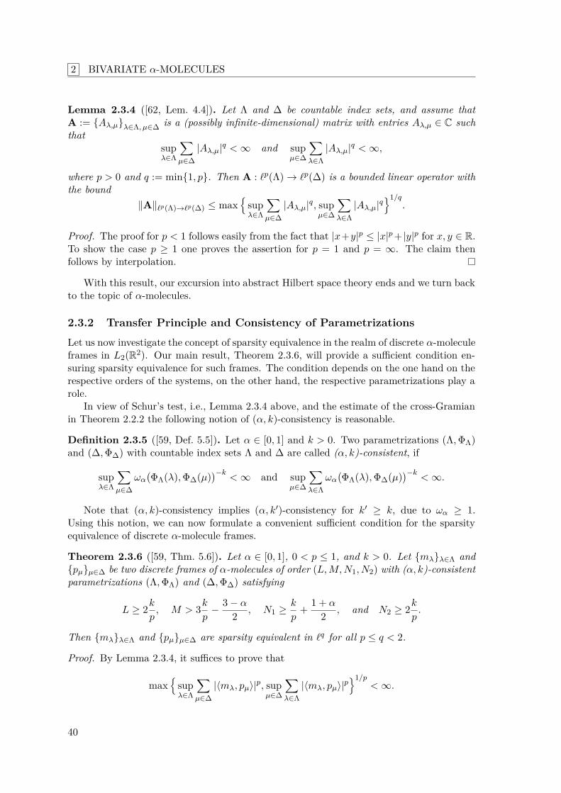
2 BIVARIATE α-MOLECULES
Lemma 2.3.4 ([62, Lem. 4.4]). Let Λ and ∆ be countable index sets, and assume thatA := Aλ,µλ∈Λ, µ∈∆ is a (possibly infinite-dimensional) matrix with entries Aλ,µ ∈ C suchthat
supλ∈Λ
µ∈∆
|Aλ,µ|q < ∞ and supµ∈∆
λ∈Λ
|Aλ,µ|q < ∞,
where p > 0 and q := min1, p. Then A : ℓp(Λ) → ℓp(∆) is a bounded linear operator withthe bound
∥A∥ℓp(Λ)→ℓp(∆) ≤ max
supλ∈Λ
µ∈∆
|Aλ,µ|q, supµ∈∆
λ∈Λ
|Aλ,µ|q1/q
.
Proof. The proof for p < 1 follows easily from the fact that |x+y|p ≤ |x|p + |y|p for x, y ∈ R.To show the case p ≥ 1 one proves the assertion for p = 1 and p = ∞. The claim thenfollows by interpolation.
With this result, our excursion into abstract Hilbert space theory ends and we turn backto the topic of α-molecules.
2.3.2 Transfer Principle and Consistency of Parametrizations
Let us now investigate the concept of sparsity equivalence in the realm of discrete α-moleculeframes in L2(R2). Our main result, Theorem 2.3.6, will provide a sufficient condition en-suring sparsity equivalence for such frames. The condition depends on the one hand on therespective orders of the systems, on the other hand, the respective parametrizations play arole.
In view of Schur’s test, i.e., Lemma 2.3.4 above, and the estimate of the cross-Gramianin Theorem 2.2.2 the following notion of (α, k)-consistency is reasonable.
Definition 2.3.5 ([59, Def. 5.5]). Let α ∈ [0, 1] and k > 0. Two parametrizations (Λ,ΦΛ)and (∆,Φ∆) with countable index sets Λ and ∆ are called (α, k)-consistent, if
supλ∈Λ
µ∈∆
ωαΦΛ(λ),Φ∆(µ)
−k< ∞ and sup
µ∈∆
λ∈Λ
ωαΦΛ(λ),Φ∆(µ)
−k< ∞.
Note that (α, k)-consistency implies (α, k′)-consistency for k′ ≥ k, due to ωα ≥ 1.Using this notion, we can now formulate a convenient sufficient condition for the sparsityequivalence of discrete α-molecule frames.
Theorem 2.3.6 ([59, Thm. 5.6]). Let α ∈ [0, 1], 0 < p ≤ 1, and k > 0. Let mλλ∈Λ andpµµ∈∆ be two discrete frames of α-molecules of order (L,M,N1, N2) with (α, k)-consistentparametrizations (Λ,ΦΛ) and (∆,Φ∆) satisfying
L ≥ 2kp, M > 3k
p− 3 − α
2 , N1 ≥ k
p+ 1 + α
2 , and N2 ≥ 2kp.
Then mλλ∈Λ and pµµ∈∆ are sparsity equivalent in ℓq for all p ≤ q < 2.
Proof. By Lemma 2.3.4, it suffices to prove that
max
supλ∈Λ
µ∈∆
|⟨mλ, pµ⟩|p, supµ∈∆
λ∈Λ
|⟨mλ, pµ⟩|p1/p
< ∞.
40
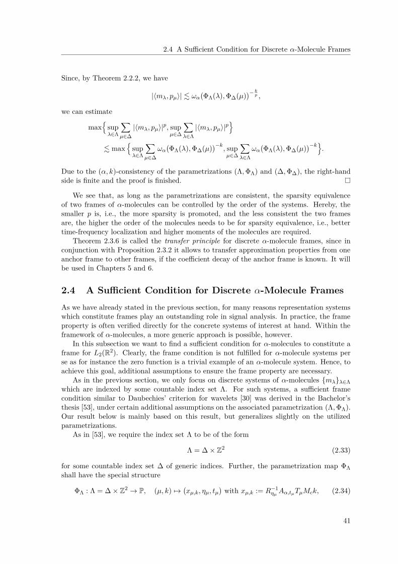
2.4 A Sufficient Condition for Discrete α-Molecule Frames
Since, by Theorem 2.2.2, we have
|⟨mλ, pµ⟩| . ωαΦΛ(λ),Φ∆(µ)
− kp ,
we can estimate
max
supλ∈Λ
µ∈∆
|⟨mλ, pµ⟩|p, supµ∈∆
λ∈Λ
|⟨mλ, pµ⟩|p
. max
supλ∈Λ
µ∈∆
ωαΦΛ(λ),Φ∆(µ)
−k, sup
µ∈∆
λ∈Λ
ωαΦΛ(λ),Φ∆(µ)
−k.
Due to the (α, k)-consistency of the parametrizations (Λ,ΦΛ) and (∆,Φ∆), the right-handside is finite and the proof is finished.
We see that, as long as the parametrizations are consistent, the sparsity equivalenceof two frames of α-molecules can be controlled by the order of the systems. Hereby, thesmaller p is, i.e., the more sparsity is promoted, and the less consistent the two framesare, the higher the order of the molecules needs to be for sparsity equivalence, i.e., bettertime-frequency localization and higher moments of the molecules are required.
Theorem 2.3.6 is called the transfer principle for discrete α-molecule frames, since inconjunction with Proposition 2.3.2 it allows to transfer approximation properties from oneanchor frame to other frames, if the coefficient decay of the anchor frame is known. It willbe used in Chapters 5 and 6.
2.4 A Sufficient Condition for Discrete α-Molecule Frames
As we have already stated in the previous section, for many reasons representation systemswhich constitute frames play an outstanding role in signal analysis. In practice, the frameproperty is often verified directly for the concrete systems of interest at hand. Within theframework of α-molecules, a more generic approach is possible, however.
In this subsection we want to find a sufficient condition for α-molecules to constitute aframe for L2(R2). Clearly, the frame condition is not fulfilled for α-molecule systems perse as for instance the zero function is a trivial example of an α-molecule system. Hence, toachieve this goal, additional assumptions to ensure the frame property are necessary.
As in the previous section, we only focus on discrete systems of α-molecules mλλ∈Λwhich are indexed by some countable index set Λ. For such systems, a sufficient framecondition similar to Daubechies’ criterion for wavelets [30] was derived in the Bachelor’sthesis [53], under certain additional assumptions on the associated parametrization (Λ,ΦΛ).Our result below is mainly based on this result, but generalizes slightly on the utilizedparametrizations.
As in [53], we require the index set Λ to be of the form
Λ = ∆ × Z2 (2.33)
for some countable index set ∆ of generic indices. Further, the parametrization map ΦΛshall have the special structure
ΦΛ : Λ = ∆ × Z2 → P, (µ, k) →→xµ,k, ηµ, tµ
with xµ,k := R−1
ηµAα,tµTµMck, (2.34)
41
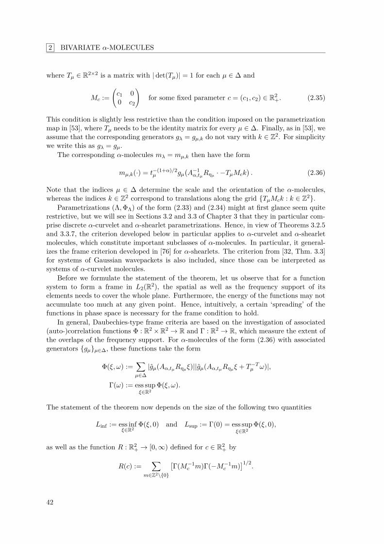
2 BIVARIATE α-MOLECULES
where Tµ ∈ R2×2 is a matrix with | det(Tµ)| = 1 for each µ ∈ ∆ and
Mc :=c1 00 c2
for some fixed parameter c = (c1, c2) ∈ R2
+. (2.35)
This condition is slightly less restrictive than the condition imposed on the parametrizationmap in [53], where Tµ needs to be the identity matrix for every µ ∈ ∆. Finally, as in [53], weassume that the corresponding generators gλ = gµ,k do not vary with k ∈ Z2. For simplicitywe write this as gλ = gµ.
The corresponding α-molecules mλ = mµ,k then have the form
mµ,k(·) = t−(1+α)/2µ gµ
A−1
α,tµRηµ · −TµMck
. (2.36)
Note that the indices µ ∈ ∆ determine the scale and the orientation of the α-molecules,whereas the indices k ∈ Z2 correspond to translations along the grid TµMck : k ∈ Z2.
Parametrizations (Λ,ΦΛ) of the form (2.33) and (2.34) might at first glance seem quiterestrictive, but we will see in Sections 3.2 and 3.3 of Chapter 3 that they in particular com-prise discrete α-curvelet and α-shearlet parametrizations. Hence, in view of Theorems 3.2.5and 3.3.7, the criterion developed below in particular applies to α-curvelet and α-shearletmolecules, which constitute important subclasses of α-molecules. In particular, it general-izes the frame criterion developed in [76] for α-shearlets. The criterion from [32, Thm. 3.3]for systems of Gaussian wavepackets is also included, since those can be interpreted assystems of α-curvelet molecules.
Before we formulate the statement of the theorem, let us observe that for a functionsystem to form a frame in L2(R2), the spatial as well as the frequency support of itselements needs to cover the whole plane. Furthermore, the energy of the functions may notaccumulate too much at any given point. Hence, intuitively, a certain ‘spreading’ of thefunctions in phase space is necessary for the frame condition to hold.
In general, Daubechies-type frame criteria are based on the investigation of associated(auto-)correlation functions Φ : R2 ×R2 → R and Γ : R2 → R, which measure the extent ofthe overlaps of the frequency support. For α-molecules of the form (2.36) with associatedgenerators gµµ∈∆, these functions take the form
Φ(ξ, ω) :=µ∈∆
|gµ(Aα,tµRηµξ)||gµ(Aα,tµRηµξ + T−Tµ ω)|,
Γ(ω) := ess supξ∈R2
Φ(ξ, ω).
The statement of the theorem now depends on the size of the following two quantities
Linf := ess infξ∈R2
Φ(ξ, 0) and Lsup := Γ(0) = ess supξ∈R2
Φ(ξ, 0),
as well as the function R : R2+ → [0,∞) defined for c ∈ R2
+ by
R(c) :=
m∈Z2\0
Γ(M−1
c m)Γ(−M−1c m)
1/2.
42
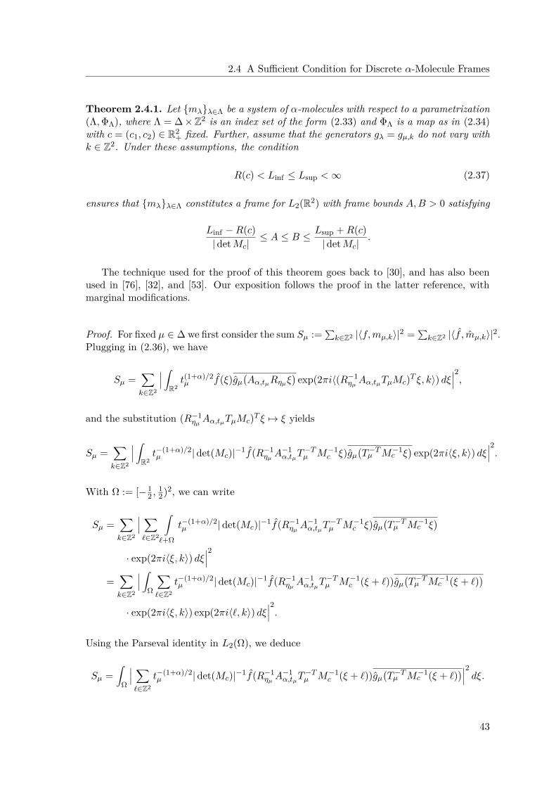
2.4 A Sufficient Condition for Discrete α-Molecule Frames
Theorem 2.4.1. Let mλλ∈Λ be a system of α-molecules with respect to a parametrization(Λ,ΦΛ), where Λ = ∆ ×Z2 is an index set of the form (2.33) and ΦΛ is a map as in (2.34)with c = (c1, c2) ∈ R2
+ fixed. Further, assume that the generators gλ = gµ,k do not vary withk ∈ Z2. Under these assumptions, the condition
R(c) < Linf ≤ Lsup < ∞ (2.37)
ensures that mλλ∈Λ constitutes a frame for L2(R2) with frame bounds A,B > 0 satisfying
Linf −R(c)| detMc|
≤ A ≤ B ≤ Lsup +R(c)| detMc|
.
The technique used for the proof of this theorem goes back to [30], and has also beenused in [76], [32], and [53]. Our exposition follows the proof in the latter reference, withmarginal modifications.
Proof. For fixed µ ∈ ∆ we first consider the sum Sµ :=
k∈Z2 |⟨f,mµ,k⟩|2 =
k∈Z2 |⟨f , mµ,k⟩|2.Plugging in (2.36), we have
Sµ =
k∈Z2
R2t(1+α)/2µ f(ξ)gµ
Aα,tµRηµξ
exp(2πi⟨(R−1
ηµAα,tµTµMc)T ξ, k⟩) dξ
2,and the substitution (R−1
ηµAα,tµTµMc)T ξ →→ ξ yields
Sµ =
k∈Z2
R2t−(1+α)/2µ | det(Mc)|−1f(R−1
ηµA−1
α,tµT−T
µ M−1c ξ)gµ
T−T
µ M−1c ξ
exp(2πi⟨ξ, k⟩) dξ
2.With Ω := [−1
2 ,12)2, we can write
Sµ =
k∈Z2
ℓ∈Z2
ℓ+Ω
t−(1+α)/2µ | det(Mc)|−1f(R−1
ηµA−1
α,tµT−T
µ M−1c ξ)gµ
T−T
µ M−1c ξ
· exp(2πi⟨ξ, k⟩) dξ
2=
k∈Z2
Ω
ℓ∈Z2
t−(1+α)/2µ | det(Mc)|−1f(R−1
ηµA−1
α,tµT−T
µ M−1c (ξ + ℓ))gµ
T−T
µ M−1c (ξ + ℓ)
· exp(2πi⟨ξ, k⟩) exp(2πi⟨ℓ, k⟩) dξ
2.Using the Parseval identity in L2(Ω), we deduce
Sµ =
Ω
ℓ∈Z2
t−(1+α)/2µ | det(Mc)|−1f(R−1
ηµA−1
α,tµT−T
µ M−1c (ξ + ℓ))gµ
T−T
µ M−1c (ξ + ℓ)
2 dξ.
43
2 BIVARIATE α-MOLECULES
We continue with
Sµ =
Ωt−(1+α)µ | det(Mc)|−2
k,ℓ∈Z2
f(R−1ηµA−1
α,tµT−T
µ M−1c (ξ + k))gµ
T−T
µ M−1c (ξ + k)
· f(R−1
ηµ A−1α,tµ
T−Tµ M−1
c (ξ + ℓ))gµT−T
µ M−1c (ξ + ℓ)
dξ
=ℓ∈Z2
ℓ+Ω
t−(1+α)µ | det(Mc)|−2
k∈Z2
f(R−1ηµA−1
α,tµT−T
µ M−1c (ξ + k − ℓ))
· gµT−T
µ M−1c (ξ + k − ℓ)
f(R−1
ηµ A−1α,tµ
T−Tµ M−1
c ξ)gµT−T
µ M−1c ξ
dξ
=R2
m∈Z2
t−(1+α)µ | detMc|−2f(R−1
ηµA−1
α,tµT−T
µ M−1c ξ)gµ
T−T
µ M−1c ξ
· f(R−1
ηµ A−1α,tµ
T−Tµ M−1
c (ξ +m))gµT−T
µ M−1c (ξ +m)
.
Finally, we substitute R−1ηµA−1
α,tµT−T
µ M−1c ξ →→ ξ and arrive at
Sµ = | detMc|−1R2
m∈Z2
f(ξ)gµAα,tµRηµξ
· f(ξ +R−1
ηµ A−1α,tµ
T−Tµ M−1
c m)gµAα,tµRηµξ + T−T
µ M−1c m
.
Now we take the sum over µ ∈ ∆ and splitµ∈∆
Sµ = T1 + T2
into a term T1, corresponding to m = 0,
T1 := | detMc|−1R2
µ∈∆
|f(ξ)|2|gµAα,tµRηµξ
|2 dξ,
and a term T2, corresponding to m = 0,
T2 := | detMc|−1R2
µ∈∆
m∈Z2\0
f(ξ)f(ξ +R−1ηµ A
−1α,tµ
T−Tµ M−1
c m)
· gµAα,tµRηµξ
gµAα,tµRηµξ + T−T
µ M−1c m
dξ.
Using the definition of Linf and Lsup, we directly obtain for T1
Linf| det(Mc)|
∥f∥2 ≤ T1 ≤ Lsup| det(Mc)|
∥f∥2. (2.38)
Further, for T2 we will prove
|T2| ≤ R(c)| det(Mc)|
∥f∥2. (2.39)
For this, we first estimate
|T2| ≤ | detMc|−1 m∈Z2\0
R2
µ∈∆
|f(ξ)|gµAα,tµRηµξ
gµAα,tµRηµξ + T−T
µ M−1c m
1/2
· |f(ξ +R−1ηµA−1
α,tµT−T
µ M−1c m)|
gµAα,tµRηµξ
gµAα,tµRηµξ + T−T
µ M−1c m
1/2dξ.
44
2.5 Appendix: Proof of Theorem 2.2.2
Then we proceed with a double application of the Cauchy-Schwarz inequality, first to thesum and then to the integral. We obtain
|T2| ≤ | detMc|−1 m∈Z2\0
R2
µ∈∆
|f(ξ)|2|gµAα,tµRηµξ
||gµ
Aα,tµRηµξ + T−T
µ M−1c m
| dξ
1/2
·
R2
µ∈∆
|f(ξ +R−1ηµA−1
α,tµT−T
µ M−1c m)|2|gµ
Aα,tµRηµξ
gµAα,tµRηµξ + T−T
µ M−1c m
| dξ
1/2.
Finally, we substitute ξ + R−1ηµA−1
α,tµT−T
µ M−1c n →→ ξ in the second integral and arrive at
(2.39), namely
|T2| ≤ | detMc|−1 m∈Z2\0
R2
|f(ξ)|2µ∈∆
|gµAα,tµRηµξ
gµAα,tµRηµξ + T−T
µ M−1c m
| dξ
1/2
·
R2|f(ξ)|2
µ∈∆
|gµAα,tµRηµξ
gµAα,tµRηµξ − T−T
µ M−1c m
| dξ
1/2
≤ | detMc|−1∥f∥2 m∈Z2\0
Γ(M−1
c m)Γ(−M−1c m)
1/2= R(c)
| detMc|∥f∥2.
Altogether, the estimates (2.38) and (2.39) imply
Linf −R(c)| det(Mc)|
∥f∥2 ≤µ∈∆
Sµ ≤ Lsup +R(c)| det(Mc)|
∥f∥2,
which finishes the proof.
Concerning the application of this theorem, let us remark that, intuitively, when cgets smaller also R(c) becomes smaller. A good strategy to fulfill the condition (2.37) inTheorem 2.4.1 is thus to choose the parameter c sufficiently small. This strategy was usedfor example in [76] to confirm the frame property of the constructed compactly supportedshearlets.
In the next chapter, where we will investigate specific instances of α-molecule systems,we will use this theorem to deduce sufficient frame criteria for α-curvelet and α-shearletmolecules.
2.5 Appendix: Proof of Theorem 2.2.2In the following, we reproduce the proof of Theorem 2.2.2 given in [59], whereby the no-tation is adapted to our setting and some minor inaccuracies are corrected. We start bycollecting some useful lemmata in Subsections 2.5.1–2.5.3, followed by the actual proof inSubsection 2.5.4.
2.5.1 General Estimates
Let us recall the projective bracket introduced in (2.9). An important property of thisbracket is given by the following lemma.
45
2 BIVARIATE α-MOLECULES
Lemma 2.5.1. For θ ∈ R let θ denote its ‘projection’ onto the interval T := [−π2 ,
π2 ) as
introduced in (2.9). It then holds |θ| ≍ | sin(θ)|.
Proof. Due to π-periodicity it suffices to verify the relation for θ ∈ [−π2 ,
π2 ). In this range
we have 2π |θ| ≤ | sin(θ)| ≤ |θ|.
The following lemma can be found in [51, Appendix K.1].
Lemma 2.5.2. For N > 1 and a, a′ ∈ R+, we have the inequalityR
(1 + a|x|)−N 1 + a′|x− y|−N
dx . maxa, a′−1(1 + mina, a′|y|)−N .
The implicit constant is independent of a, a′ and y ∈ R.
The following result can be regarded as a corollary of the previous lemma.
Lemma 2.5.3. Assume that η ∈ R and N > 1. Then we have for a, a′ ∈ R+ the inequalityT
(1 + a| sin(ϕ)|)−N 1 + a′| sin(ϕ+ η)|−N
dϕ . maxa, a′−1(1 + mina, a′|η|)−N .
(2.40)The implicit constant is independent of a, a′ and η ∈ R.
Proof. Let T := [−π/2, π/2). Using the π-periodicity of the integrand and the equivalence| sin(ϕ)| ≍ |ϕ|, where ϕ ∈ R and · = ·T is the projective bracket defined in (2.9), weobtain
T(1 + a| sin(ϕ)|)−N 1 + a′| sin(ϕ+ η)|
−Ndϕ
≍
T(1 + a| sin(ϕ)|)−N 1 + a′| sin(ϕ+ η)|
−Ndϕ
≍
T(1 + a|ϕ|)−N 1 + a′|ϕ+ η|
−Ndϕ.
The left-hand side of (2.40) can thus be estimated by a constant times
θ∈0,±π
R
(1 + a|ϕ|)−N 1 + a′|ϕ+ η + θ|−N
dϕ,
where we used ϕ+η = ϕ+η. Further, by Lemma 2.5.2 and since |η+θ| ≤ |η+θ|,this sum is bounded by a constant times
θ∈0,±πmaxa, a′−1(1 + mina, a′|η + θ|)−N .
It remains to note that for θ ∈ 0,±π we have |η+θ| = |η|. This proves the lemma.
46
2.5 Appendix: Proof of Theorem 2.2.2
2.5.2 Basic Estimates of Sλ,M,N1,N2
We now consider the function Sλ,M,N1,N2 : [0,∞)×[0, 2π) → R for λ ∈ Λ andM,N1, N2 ∈ N0which is defined in polar coordinates by
Sλ,M,N1,N2(r, ϕ) := min
1, tλ(1 + r)M
1 + t−(1−α)λ | sin(ϕ+ ηλ)|
−N21 + tλr
−N1.
The reader might want to compare this definition with (2.6).The following lemma will be used in order to decouple the angular and the radial vari-
ables.
Lemma 2.5.4. For every 0 ≤ K ≤ N2,
min
1, tλ(1 + r)M
1 + tλr−N1
1 + tαλr| sin(ϕ+ ηλ)|−N2
. Sλ,M−K,N1,K(r, ϕ).
Proof. After choosing K, we can estimate the quantity on the left hand side by
min 1, tλ(1 + r)M−K (1 + tλr)−N1
min 1, tλ(1 + r)
1 + tαλr| sin(ϕ+ ηλ)|
K
.
We need to show that
min 1, tλ(1 + r)1 + tαλr| sin(ϕ+ ηλ)| .
1 + t
−(1−α)λ | sin(ϕ+ ηλ)|
−1. (2.41)
In order to prove (2.41), we distinguish three cases:
• r ≤ 1: For r ≤ 1 we have
min 1, tλ(1 + r)1 + tαλr| sin(ϕ+ ηλ)| . min 1, tλ .
1 + t
−(1−α)λ | sin(ϕ+ ηλ)|
−1.
• t−1λ ≤ r: In this case we derive
min 1, tλ(1 + r)1 + tαλr| sin(ϕ+ ηλ)| = 1
1 + tαλr| sin(ϕ+ ηλ)| ≤ 11 + tαλt
−1λ | sin(ϕ+ ηλ)|
=1 + t
−(1−α)λ | sin(ϕ+ ηλ)|
−1.
If t−1λ > 1 we have to examine a third case.
• 1 < r < t−1λ : In this case we have
min 1, tλ(1 + r)1 + tαλr| sin(ϕ+ ηλ)| ≤ tλ(1 + r)
1 + tαλr| sin(ϕ+ ηλ)| = 1 + r
r
1r−1t−1
λ + t−(1−α)λ | sin(ϕ+ ηλ)|
.
Since r > 1, we have 1+rr < 2, and since r < t−1
λ , also r−1t−1λ > 1 holds.
This proves the statement.
47
2 BIVARIATE α-MOLECULES
The next lemma provides estimates for the inner product of two functions of the formSλ,M,N1,N2 .
Lemma 2.5.5. We assume tλ, tµ ≤ C < ∞ for all λ ∈ Λ and µ ∈ ∆. For A,B ≥ 1 and
N1 ≥ A+ 1 + α
2 , N2 ≥ B, M > N1 − 2,
we have if N1 > 1
(tλtµ)1+α
2
R+
TSλ,M,N1,N2(r, ϕ)Sµ,M,N1,N2(r, ϕ)rdϕdr
. max tλtµ,tµtλ
−A 1 + maxtλ, tµ−(1−α)|ηλ − ηµ|
−B.
Proof. We assume without loss of generality that tλ ≥ tµ and start by proving the angulardecay. An application of Lemma 2.5.3 yields
T
1 + t
−(1−α)λ | sin(ϕ+ ηλ)|
−N21 + t−(1−α)
µ | sin(ϕ+ ηµ)|−N2
dϕ
. t1−αµ
1 + t
−(1−α)λ |ηλ − ηµ|
−N2.
Taking into account N2 ≥ B ≥ 1, we thus obtain
(tλtµ)1+α
2
R+
TSλ,M,N1,N2(r, ϕ)Sµ,M,N1,N2(r, ϕ)rdϕdr
. S · tλtµ
1+α21 + t
−(1−α)λ |ηλ − ηµ|
−B,
where
S := t2µ
R+
min 1, tλ(1 + r)M min 1, tµ(1 + r)M (1 + tλr)−N1 (1 + tµr)−N1 rdr.
The remaining estimate
S . (tλ/tµ)−(A+ 1+α2 ) (2.42)
is proved by splitting up the integral into the three parts Si, i = 1, 2, 3, where the integrationranges over 0 < r < 1, 1 ≤ r ≤ max1, t−1
µ and max1, t−1µ < r, respectively.
Case 1 (0 < r < 1): For S1 we integrate over 0 < r < 1. Here we use the moment propertyand t−1
λ ≥ 1/C > 0 to estimate
S1 . t2µ
1
0tMλ tMµ dr
= t2+Mµ tMλ
. t2+Mµ t
−(M+2)λ
= (tµ/tλ)M+2
≤ (tµ/tλ)A+ 1+α2 .
48
2.5 Appendix: Proof of Theorem 2.2.2
Case 2 (1 ≤ r ≤ max1, t−1µ ): If t−1
µ ≤ 1 then S2 = 0. For t−1µ > 1 we estimate
S2 . t2µ
t−1µ
1(tµr)M (tλr)−N1 rdr
≤ t2+Mµ t−N1
λ
t−1µ
0rM+1−N1dr
. t2+Mµ t−N1
λ t−(M+2−N1)µ
= (tµ/tλ)N1
≤ (tµ/tλ)A+ 1+α2 .
Case 3 (max1, t−1µ < r): For S3 we estimate
S3 . t2µ
∞
t−1µ
(tλr)−N1 (tµr)−N1 rdr
= t2µt−N1µ t−N1
λ
∞
t−1µ
r−2N1+1dr
. t2µt−N1µ t−N1
λ t2N1−2µ
= (tµ/tλ)N1
≤ (tµ/tλ)A+ 1+α2 .
Altogether, this establishes (2.42).
2.5.3 Estimates with Differential Operator
Finally, we require some estimates involving the symmetric differential operator Lλ,µ (actingon the frequency variable ξ ∈ R2) defined for λ ∈ Λ and µ ∈ ∆ by
Lλ,µ := I − t−2α0 ∆ξ − t−2
0
1 + t−2(1−α)0 |δη|2
⟨eλ,∇⟩2, (2.43)
where δη := ηλ − ηµ and t0 := maxtλ, tµ. The first lemma is an auxiliary result.
Lemma 2.5.6. Assume that the assumptions of Theorem 2.2.2 hold true for two systems ofα-molecules of order (L,M,N1, N2) with respective generators a(λ)λ and b(µ)µ. Givenany two of those generators a(λ), b(µ), the expression
Lλ,µ
a(λ) (Aα,tλ
Rηλξ) b(µ) Aα,tµRηµξ
can be written as a finite linear combination of terms of the form
c(λ) (Aα,tλRηλ
ξ) d(µ) Aα,tµRηµξ,
with c(λ), d(µ) satisfying (2.5) for L− 2,M,N1, N2 with an implicit constant independent ofλ and µ. Thereby, the number of terms in the linear combinations and the correspondingcoefficients are also uniformly bounded in λ and µ.
49
2 BIVARIATE α-MOLECULES
Proof. To prove the claim we treat the three summands of the operator Lλ,µ separately.The first part is the identity, and therefore the statement is trivial. To handle the secondpart, the frequency Laplacian t−2α
0 ∆, we use the product rule
∆(fg) = 2∂(1,0)f∂(1,0)g + ∂(0,1)f∂(0,1)g
+ (∆f)g + f(∆g).
Therefore we need to estimate the derivatives of degree 1 and the Laplacians of the twofactors in the product
a(λ) (Aα,tλRηλ
ξ) b(µ) Aα,tµRηµξ
=: A(ξ)B(ξ).
For this, we start with the first factor,
A(ξ) = a(λ) (tλ cos(ηλ)ξ1 − tλ sin(ηλ)ξ2, tαλ sin(ηλ)ξ1 + tαλ cos(ηλ)ξ2) .
Let us set
A1(ξ) :=∂(1,0)a(λ) (Aα,tλ
Rηλξ) and A2(ξ) :=
∂(0,1)a(λ) (Aα,tλ
Rηλξ) .
By definition, the functions ∂(1,0)a(λ), ∂(0,1)a(λ) satisfy (2.5) with L replaced by L− 1. Anapplication of the chain rule shows that
∂(1,0)A(ξ) = tλ cos(ηλ)A1(ξ) + tαλ sin(ηλ)A2(ξ).
Analogously, one can compute
∂(0,1)A(ξ) = −tλ sin(ηλ)A1(ξ) + tαλ cos(ηλ)A2(ξ),
and the exact same expressions for B using the obvious definitions for B1 and B2. We get
∂(1,0)A∂(1,0)B = tλtµ cos(ηλ) cos(ηµ)A1B1 + tαλtµ sin(ηλ) cos(ηµ)A2B1
+tαµtλ sin(ηµ) cos(ηλ)A1B2 + (tλtµ)α sin(ηλ) sin(ηµ)A2B2.
It follows that t−2α0 ∂(1,0)A∂(1,0)B can be written as a linear combination as claimed (recall
that t0 = maxtλ, tµ). The same argument applies to the product t−2α0 ∂(0,1)A∂(0,1)B.
It remains to consider the factor
(∆A)B +A(∆B),
where, for symmetry reasons, we only treat the summand (∆A)B. In fact, it suffices toonly consider
(∂(2,0)A)B =t2λ cos(ηλ)2A11 + 2t1+α
λ sin(ηλ) cos(ηλ)A12 + t2αλ sin(ηλ)2A22
B (2.44)
with Aij , i, j ∈ 1, 2, defined in the obvious way, and where ∂(2,0)a(λ), ∂(1,1)a(λ), and∂(0,2)a(λ) satisfy (2.5) with L replaced by L − 2. The term (∂(0,2)A)B, and hence (∆A)B,can be handled in the same way, as can A(∆B). This takes care of the term t−2α
0 ∆ in thedefinition of Lλ,µ.
50
2.5 Appendix: Proof of Theorem 2.2.2
Finally, we need to handle the last term in the definition of Lλ,µ, namely
t−20
1 + t−2(1−α)0 |ηµ|2
∂2
∂ξ21
for ηλ = 0 (otherwise the second order derivative would be in the direction of the unit vectorwith angle ηλ with obvious modifications in the proof). With our notation and using theproduct rule we need to consider terms of the form
(∂(2,0)A)B, (∂(1,0)A)(∂(1,0)B), A(∂(2,0)B),
and show that each of them, multiplied by the factor t−20 /(1 + t
−2(1−α)0 |ηµ|2), possesses
the desired representation.Let us start with (∂(2,0)A)B, which, using (2.44) and the fact that ηλ = 0, can be written
as(∂(2,0)A)B = t2λA11B,
and which clearly satisfies the desired assertion.Now consider the expression (∂(1,0)A)(∂(1,0)B), which can be written as
(∂(1,0)A)(∂(1,0)B) = tλtµ cos(ηµ)A1B1 + tλtαµ sin(ηµ)A1B2.
The first summand in this expression clearly causes no problems. To handle the secondterm we need to show that
t−20
1 + t−2(1−α)0 |ηµ|2
tλtαµ| sin(ηµ)| . 1. (2.45)
Here we have to distinguish two cases. First, assume that |ηµ| ≤ t1−α0 . Then we can
estimate | sin(ηµ)| ≤ t1−α0 , which readily yields the desired bound for (2.45). For the case
|ηµ| ≥ t1−α0 we estimate
t−20
1 + t−2(1−α)0 |ηµ|2
tλtαµ| sin(ηµ)| ≤ t−2
0
1 + t−(1−α)0 |ηµ|
t0tα0 |ηµ| ≤ t−2
0
t−(1−α)0 |ηµ|
t0tα0 |ηµ| = 1
which proves (2.45) also for this case.We are left with estimating the term A
∂(2,0)B
, which, similar to (2.44), can be written
ast2µ cos(ηµ)2AB11 + 2t1+α
µ sin(ηµ) cos(ηµ)AB12 + t2αµ sin(ηµ)2AB22.
The first two terms are of a form already treated, and the last term can be handled usingthe fact that | sin(ηµ)|2 ≤ |ηµ|2.
Lemma 2.5.7. Assume that the assumptions of Theorem 2.2.2 hold for two systems of α-molecules of order (L,M,N1, N2) with respective generating functions a(λ)λ and b(µ)µ.Then we have
Lkλ,µ
a(λ) (Aα,tλ
Rηλξ) b(µ) Aα,tµRηµξ
. Sλ,M−N2,N1,N2(ξ)Sµ,M−N2,N1,N2(ξ)
for all k ≤ L/2.
51
2 BIVARIATE α-MOLECULES
Proof. We show thatLkλ,µ
a(λ) (Aα,tλ
Rηλξ) b(µ) Aα,tµRηµξ
. min 1, tλ(1 + r)M (1 + tλr)−N1 (1 + tαλr| sin(ϕ+ ηλ)|)−N2
· min 1, tµ(1 + r)M (1 + tµr)−N11 + tαµr| sin(ϕ+ ηµ)|
−N2 (2.46)
which, using Lemma 2.5.4 with K = N2, implies the desired statement.To prove (2.46), we use induction in k, namely we show that if we have two functions
a(λ), b(µ) satisfying (2.5) for L,M,N1, N2, then the expression
Lλ,µ
a(λ) (Aα,tλ
Rηλξ) b(µ) Aα,tµRηµξ
can be written as a finite linear combination of terms of the form
c(λ) (Aα,tλRηλ
ξ) d(µ) Aα,tµRηµξ
with c(λ), d(µ) satisfying (2.5) and L replaced by L − 2, see Lemma 2.5.6. Iterating thisargument we can establish that for k ≤ L/2
Lkλ,µ
a(λ) (Aα,tλ
Rηλξ) b(µ) Aα,tµRηµξ
(2.47)
can be expressed as a finite linear combination of terms of the form
c(λ) (Aα,tλRηλ
ξ) d(µ) Aα,tµRηµξ
(2.48)
with c(λ)(ξ) . min
1, tλ + |ξ1| + t1−α
λ |ξ2|M
⟨|ξ|⟩−N1 ⟨ξ2⟩−N2 , (2.49)
and an analogous estimate for d(µ). Combining (2.48) and (2.49), we obtain that |(2.47)|can – up to a constant – be upperbounded by the product of
min
1, tλ +[Aα,tλ
Rηλξ]1+ t1−α
λ
[Aα,tλRηλ
ξ]2M
⟨|Aα,tλRηλ
ξ|⟩−N1[Aα,tλ
Rηλξ]2−N2
and
min
1, tµ +Aα,tµRηµξ
1
+ t1−αµ
Aα,tµRηµξ2
M Aα,tµRηµξ−N1
Aα,tµRηµξ
2
−N2.
Transforming this inequality into polar coordinates as in (2.6) yields (2.46). This finishesthe proof.
2.5.4 Actual Proof of Theorem 2.2.2
We now have all the ingredients to prove Theorem 2.2.2. By our assumptions on the order(L,M,N1, N2), there exist N1 and N2 such thatN1 ≥ N1 ≥ N+1+α
2 andN2 ≥ N2 ≥ N+1+α2
and M > N1 + N2 − 2. The systems mλλ and pµµ are also α-molecules of order(L,M, N1, N2), satisfying the assumptions of the theorem. Thus, we can without loss ofgenerality assume the additional condition M > N1 +N2 − 2.
52
2.5 Appendix: Proof of Theorem 2.2.2
To keep the notation simple, we assume that ηλ = 0 and define t0 := maxtλ, tµ.Further, we set
δx := xλ − xµ, δη := ηλ − ηµ.
By definition, we can write
mλ(·) = t− 1+α
2λ a(λ)
A−1
α,tλRηλ
(· − xλ), pµ(·) = t
− 1+α2
µ b(µ)A−1
α,tµRηµ(· − xµ)
,
where both a(λ) and b(µ) satisfy (2.5). We have the equality
⟨mλ, pµ⟩ = ⟨mλ, pµ⟩
= (tλtµ)1+α
2
R2a(λ) (Aα,tλ
Rηλξ) b(µ) Aα,tµRηµξ
exp (−2πiξ · δx) dξ (2.50)
= (tλtµ)1+α
2
R2
Lkλ,µ
a(λ) (Aα,tλ
Rηλξ) b(µ) Aα,tµRηµξ
L−k
λ,µ (exp (−2πiξ · δx)) dξ,
where Lλ,µ is the symmetric differential operator (acting on the frequency variable) definedin (2.43). Note that by assumption N1 > 1 and thus the boundary terms vanish due to thedecay properties of a(λ) and b(µ) as well as their derivatives.
We have
L−kλ,µ (exp (−2πiξ · δx)) =
1 + t−2α
0 |δx|2 + t−20
1 + t−2(1−α)0 |δη|
⟨eλ, δx⟩2−k
exp (−2πiξ · δx) ,
(2.51)where eλ = (cos(ηλ),− sin(ηλ)) denotes the unit vector pointing in the direction describedby the angle ηλ. By Lemma 2.5.7 and for k ≤ L
2 , we have the inequality
Lkλ,µ
a(λ) (Aα,tλ
Rηλξ) b(µ) Aα,tµRηµξ
. Sλ,M−N2,N1,N2(ξ)Sµ,M−N2,N1,N2(ξ).
Then, by (2.50) and (2.51) it follows that
|⟨mλ, pµ⟩| . (tλtµ)1+α
2
R2Sλ,M−N2,N1,N2(ξ)Sµ,M−N2,N1,N2(ξ)dξ
·
1 + t−2α0 |δx|2 + t−2
0
1 + t−2(1−α)0 |δη|
⟨eλ, δx⟩2−k
for all k ≤ L2 . Now we can use Lemma 2.5.5 and the fact that L ≥ 2N to establish that
|⟨mλ, pµ⟩| . max tλtµ,tµtλ
−N 1 + t
−2(1−α)0 |δη|2
−N
·
1 + t−2α0 |δx|2 + t−2
0
1 + t−2(1−α)0 |δη|
⟨eλ, δx⟩2−N
≤ max tλtµ,tµtλ
−N
1 + t−2(1−α)0 |δη|2 + t−2α
0 |δx|2 + t−20
1 + t−2(1−α)0 |δη|
⟨eλ, δx⟩2−N
= ωαΦΛ(λ),Φ∆(µ)
−N.
This proves the desired statement.
53

54
Chapter 3
Examples of α-Molecules in L2(R2)
In this chapter we will fill the abstract notion of α-molecules from Definition 2.1.3 with lifeby presenting a few prominent examples of specific α-molecule systems. Undoubtedly, themost natural examples are given by curvelet systems since the construction of those servedas a guiding principle for the α-molecule definition. But, as we will see in this chapter, alsowavelet systems, ridgelet systems and even shear-based constructions fit into the frame-work. Two important subclasses of α-molecule systems, namely α-curvelet and α-shearletmolecules, are distinguished, and we will show that their associated parametrizations areconsistent in a suitable sense.
3.1 Continuous α-Curvelets
We begin our exposition with a prototypical instance of a continuous α-molecule frame forL2(R2). Guided by the construction of the parabolically scaled curvelets in [11], we willconstruct a continuous Parseval frame of α-curvelets for every α ∈ [0, 1]. The obtainedsystems, denoted by Cα, are band-limited and based on a specific tiling of the frequencydomain.
To realize this tiling, let us first define two radial functions U,U1 ∈ C∞c ([0,∞)) which
shall be nonnegative and satisfy
suppU ⊂ (12 , 2) and suppU1 ⊂ [0, 2) .
Further, they shall fulfill the continuous Calderón condition
U21 (r) +
1
0U(rt)2dt
t= 1 for all r ≥ 0 . (3.1)
Next, let us take a non-negative angular function V ∈ C∞c ([−π, π]) with the property
suppV ⊂ (−1, 1) and 1
−1V (η)2 dη = 1 .
Further, for convenience, let us also introduce the constant function V1 : [−π, π] → 1√2π
.Now we are ready to define the functions Wη,t ∈ C∞
c (R2), where η ∈ T = [0, 2π)and t ∈ (0, 1], which correspond to the desired frequency tiling. Using polar coordinatesξ(r, φ) = (r cos(φ), r sin(φ)) ∈ R2 with r ∈ R+
0 := [0,∞) and φ ∈ [0, 2π), we put
Wη,1ξ(r, φ)
:= U1(r)V1(φ2T) = 1√
2πU1(r) , η ∈ T, t = 1,
Wη,tξ(r, φ)
:= U(tr)V
tα−1φ+ η2T
, η ∈ T, 0 < t < 1.
(3.2)
55
3 EXAMPLES OF α-MOLECULES IN L2(R2)
Here ·2T denotes the projective bracket (2.9) for the interval 2T = [−π, π).For t = 1 the functions Wη,t are supported in a closed ball around the origin. If 0 < t < 1
their support is a wedge-like tile whose position is determined by η and t. The induced tilingresembles that of a dicrete α-curvelet frame depicted in Figure 3.1.
From Wη,t we obtain the α-curvelets ψx,η,t ∈ L2(R2) by defining on the Fourier side
ψx,η,t(·) := t(1+α)/2Wη,t(·) exp(−2πi⟨x, ·⟩) , (x, η, t) ∈ X ,
with indices from the curvelet domain
X := R2 × T × (0, 1].
Note that, due to the normalization factor, the α-curvelets ψx,η,t are L2-normalized.Further, they are Schwartz functions, i.e., ψx,η,t ∈ S(R2). Due to the lack of symmetry ofWη,t, however, they are not real-valued as the discrete parabolic curvelets in [15].
On the spatial side, the α-curvelets can be represented in the form
ψx,η,t(·) = ψ0,0,tRη(· − x)
with ψ0,0,t = t(1+α)/2W0,t , (x, η, t) ∈ X, (3.3)
where Rη is the rotation matrix (2.3) given by
Rη =
cos(η) − sin(η)sin(η) cos(η)
, η ∈ R. (3.4)
Altogether, the constructed α-curvelets constitute a continuous multi-scale system inL2(R2) for which we subsequently use the notation
Cα :=ψx : x ∈ X
.
This system is inhomogeneous, consisting of a high-scale and a low-scale part correspondingto parameters 0 < t < 1 and t = 1, respectively. The index set X is split accordingly into ahomogeneous and an inhomogeneous component, namely
X0 := R2 × T × (0, 1) and X1 := R2 × T × 1.
Each of the components X0 and X1 is equipped with the usual product topology, whereasX is topologized as the disconnected union of the two. With this topology, X becomes alocally compact Hausdorff space.
We next search for a Radon measure, i.e., a regular Borel measure, µ on X such thatx →→ ψx is weakly measurable, i.e., the assignment x →→ ⟨f, ψx⟩ is measurable for everyf ∈ L2(R2), and such that the continuous Parseval identity is true, i.e.,
∥f |L2∥2 =X
|⟨f, ψx⟩|2 dµ(x) for all f ∈ L2(R2) . (3.5)
Note that the weak measurability is needed for the integral in (3.5) to be well-defined.With respect to µ, the system Cα is then a continuous Parseval frame for L2(R2) (see
[1]). In particular, the reconstruction formula
f =X
⟨f, ψx⟩ψx dµ(x) (3.6)
56
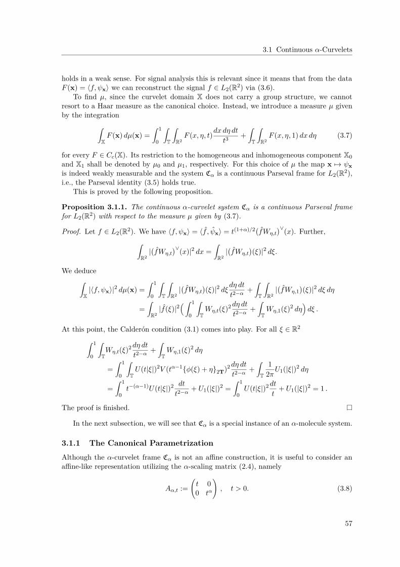
3.1 Continuous α-Curvelets
holds in a weak sense. For signal analysis this is relevant since it means that from the dataF (x) = ⟨f, ψx⟩ we can reconstruct the signal f ∈ L2(R2) via (3.6).
To find µ, since the curvelet domain X does not carry a group structure, we cannotresort to a Haar measure as the canonical choice. Instead, we introduce a measure µ givenby the integration
XF (x) dµ(x) =
1
0
T
R2F (x, η, t)dx dη dt
t3+T
R2F (x, η, 1) dx dη (3.7)
for every F ∈ Cc(X). Its restriction to the homogeneous and inhomogeneous component X0and X1 shall be denoted by µ0 and µ1, respectively. For this choice of µ the map x →→ ψxis indeed weakly measurable and the system Cα is a continuous Parseval frame for L2(R2),i.e., the Parseval identity (3.5) holds true.
This is proved by the following proposition.
Proposition 3.1.1. The continuous α-curvelet system Cα is a continuous Parseval framefor L2(R2) with respect to the measure µ given by (3.7).
Proof. Let f ∈ L2(R2). We have ⟨f, ψx⟩ = ⟨f , ψx⟩ = t(1+α)/2fWη,t∨(x). Further,
R2|fWη,t
∨(x)|2 dx =R2
|fWη,t
(ξ)|2 dξ.
We deduceX
|⟨f, ψx⟩|2 dµ(x) = 1
0
T
R2
|fWη,t
(ξ)|2 dξ dη dt
t2−α+T
R2
|fWη,1
(ξ)|2 dξ dη
=R2
|f(ξ)|2 1
0
TWη,t(ξ)2dη dt
t2−α+TWη,1(ξ)2 dη
dξ .
At this point, the Calderón condition (3.1) comes into play. For all ξ ∈ R2
1
0
TWη,t(ξ)2dη dt
t2−α+TWη,1(ξ)2 dη
= 1
0
TU(t|ξ|)2V (tα−1φ(ξ) + η2T)2dη dt
t2−α+T
12πU1(|ξ|)2 dη
= 1
0t−(α−1)U(t|ξ|)2 dt
t2−α+ U1(|ξ|)2 =
1
0U(t|ξ|)2dt
t+ U1(|ξ|)2 = 1 .
The proof is finished.
In the next subsection, we will see that Cα is a special instance of an α-molecule system.
3.1.1 The Canonical Parametrization
Although the α-curvelet frame Cα is not an affine construction, it is useful to consider anaffine-like representation utilizing the α-scaling matrix (2.4), namely
Aα,t :=t 00 tα
, t > 0. (3.8)
57
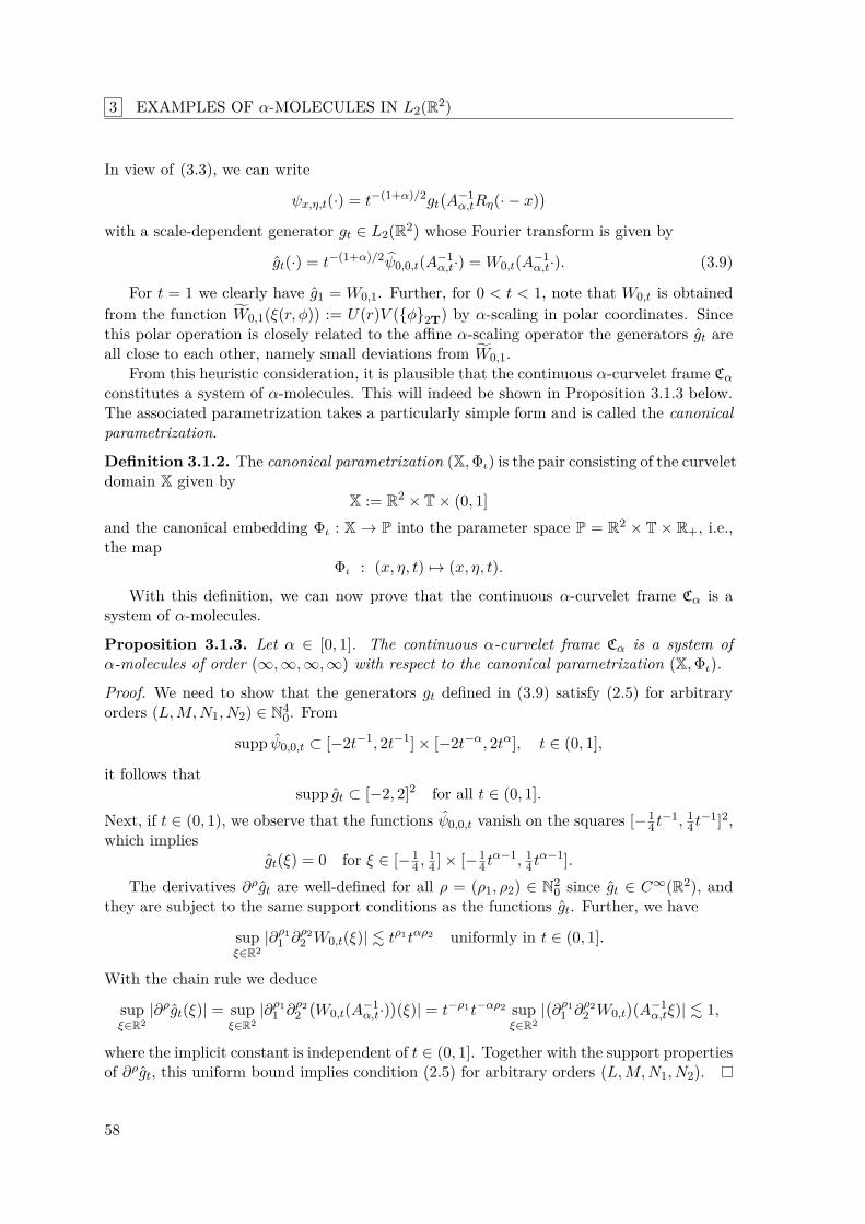
3 EXAMPLES OF α-MOLECULES IN L2(R2)
In view of (3.3), we can write
ψx,η,t(·) = t−(1+α)/2gtA−1
α,tRη(· − x)
with a scale-dependent generator gt ∈ L2(R2) whose Fourier transform is given by
gt(·) = t−(1+α)/2 ψ0,0,t(A−1α,t·) = W0,t(A−1
α,t·). (3.9)
For t = 1 we clearly have g1 = W0,1. Further, for 0 < t < 1, note that W0,t is obtainedfrom the function W0,1(ξ(r, φ)) := U(r)V (φ2T) by α-scaling in polar coordinates. Sincethis polar operation is closely related to the affine α-scaling operator the generators gt areall close to each other, namely small deviations from W0,1.
From this heuristic consideration, it is plausible that the continuous α-curvelet frame Cα
constitutes a system of α-molecules. This will indeed be shown in Proposition 3.1.3 below.The associated parametrization takes a particularly simple form and is called the canonicalparametrization.
Definition 3.1.2. The canonical parametrization (X,Φι) is the pair consisting of the curveletdomain X given by
X := R2 × T × (0, 1]and the canonical embedding Φι : X → P into the parameter space P = R2 × T × R+, i.e.,the map
Φι : (x, η, t) →→ (x, η, t).
With this definition, we can now prove that the continuous α-curvelet frame Cα is asystem of α-molecules.
Proposition 3.1.3. Let α ∈ [0, 1]. The continuous α-curvelet frame Cα is a system ofα-molecules of order (∞,∞,∞,∞) with respect to the canonical parametrization (X,Φι).
Proof. We need to show that the generators gt defined in (3.9) satisfy (2.5) for arbitraryorders (L,M,N1, N2) ∈ N4
0. From
supp ψ0,0,t ⊂ [−2t−1, 2t−1] × [−2t−α, 2tα], t ∈ (0, 1],
it follows thatsupp gt ⊂ [−2, 2]2 for all t ∈ (0, 1].
Next, if t ∈ (0, 1), we observe that the functions ψ0,0,t vanish on the squares [−14 t
−1, 14 t
−1]2,which implies
gt(ξ) = 0 for ξ ∈ [−14 ,
14 ] × [−1
4 tα−1, 1
4 tα−1].
The derivatives ∂ρgt are well-defined for all ρ = (ρ1, ρ2) ∈ N20 since gt ∈ C∞(R2), and
they are subject to the same support conditions as the functions gt. Further, we have
supξ∈R2
|∂ρ11 ∂ρ2
2 W0,t(ξ)| . tρ1tαρ2 uniformly in t ∈ (0, 1].
With the chain rule we deduce
supξ∈R2
|∂ρgt(ξ)| = supξ∈R2
|∂ρ11 ∂ρ2
2W0,t(A−1
α,t·)(ξ)| = t−ρ1t−αρ2 sup
ξ∈R2|∂ρ1
1 ∂ρ22 W0,t
(A−1
α,tξ)| . 1,
where the implicit constant is independent of t ∈ (0, 1]. Together with the support propertiesof ∂ρgt, this uniform bound implies condition (2.5) for arbitrary orders (L,M,N1, N2).
58
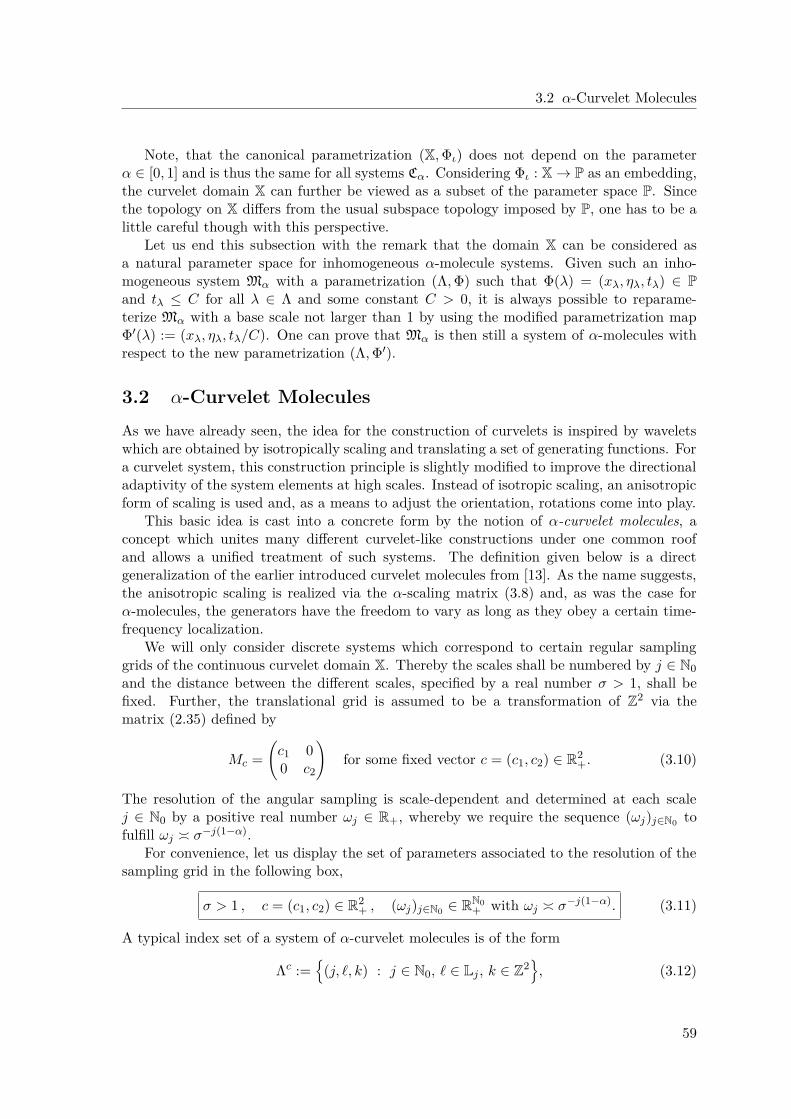
3.2 α-Curvelet Molecules
Note, that the canonical parametrization (X,Φι) does not depend on the parameterα ∈ [0, 1] and is thus the same for all systems Cα. Considering Φι : X → P as an embedding,the curvelet domain X can further be viewed as a subset of the parameter space P. Sincethe topology on X differs from the usual subspace topology imposed by P, one has to be alittle careful though with this perspective.
Let us end this subsection with the remark that the domain X can be considered asa natural parameter space for inhomogeneous α-molecule systems. Given such an inho-mogeneous system Mα with a parametrization (Λ,Φ) such that Φ(λ) = (xλ, ηλ, tλ) ∈ Pand tλ ≤ C for all λ ∈ Λ and some constant C > 0, it is always possible to reparame-terize Mα with a base scale not larger than 1 by using the modified parametrization mapΦ′(λ) := (xλ, ηλ, tλ/C). One can prove that Mα is then still a system of α-molecules withrespect to the new parametrization (Λ,Φ′).
3.2 α-Curvelet Molecules
As we have already seen, the idea for the construction of curvelets is inspired by waveletswhich are obtained by isotropically scaling and translating a set of generating functions. Fora curvelet system, this construction principle is slightly modified to improve the directionaladaptivity of the system elements at high scales. Instead of isotropic scaling, an anisotropicform of scaling is used and, as a means to adjust the orientation, rotations come into play.
This basic idea is cast into a concrete form by the notion of α-curvelet molecules, aconcept which unites many different curvelet-like constructions under one common roofand allows a unified treatment of such systems. The definition given below is a directgeneralization of the earlier introduced curvelet molecules from [13]. As the name suggests,the anisotropic scaling is realized via the α-scaling matrix (3.8) and, as was the case forα-molecules, the generators have the freedom to vary as long as they obey a certain time-frequency localization.
We will only consider discrete systems which correspond to certain regular samplinggrids of the continuous curvelet domain X. Thereby the scales shall be numbered by j ∈ N0and the distance between the different scales, specified by a real number σ > 1, shall befixed. Further, the translational grid is assumed to be a transformation of Z2 via thematrix (2.35) defined by
Mc =c1 00 c2
for some fixed vector c = (c1, c2) ∈ R2
+. (3.10)
The resolution of the angular sampling is scale-dependent and determined at each scalej ∈ N0 by a positive real number ωj ∈ R+, whereby we require the sequence (ωj)j∈N0 tofulfill ωj ≍ σ−j(1−α).
For convenience, let us display the set of parameters associated to the resolution of thesampling grid in the following box,
σ > 1 , c = (c1, c2) ∈ R2+ , (ωj)j∈N0 ∈ RN0
+ with ωj ≍ σ−j(1−α). (3.11)
A typical index set of a system of α-curvelet molecules is of the form
Λc :=
(j, ℓ, k) : j ∈ N0, ℓ ∈ Lj , k ∈ Z2, (3.12)
59
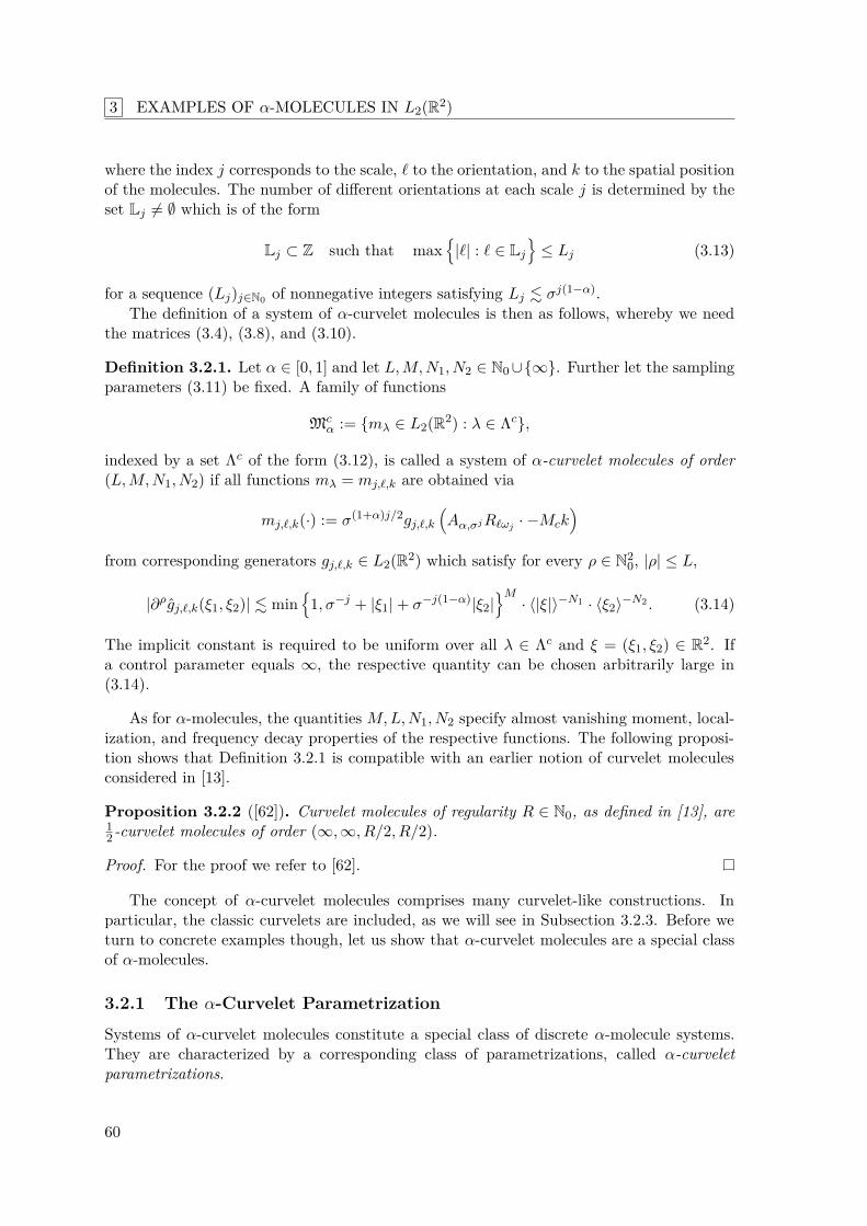
3 EXAMPLES OF α-MOLECULES IN L2(R2)
where the index j corresponds to the scale, ℓ to the orientation, and k to the spatial positionof the molecules. The number of different orientations at each scale j is determined by theset Lj = ∅ which is of the form
Lj ⊂ Z such that max
|ℓ| : ℓ ∈ Lj
≤ Lj (3.13)
for a sequence (Lj)j∈N0 of nonnegative integers satisfying Lj . σj(1−α).The definition of a system of α-curvelet molecules is then as follows, whereby we need
the matrices (3.4), (3.8), and (3.10).
Definition 3.2.1. Let α ∈ [0, 1] and let L,M,N1, N2 ∈ N0 ∪∞. Further let the samplingparameters (3.11) be fixed. A family of functions
Mcα := mλ ∈ L2(R2) : λ ∈ Λc,
indexed by a set Λc of the form (3.12), is called a system of α-curvelet molecules of order(L,M,N1, N2) if all functions mλ = mj,ℓ,k are obtained via
mj,ℓ,k(·) := σ(1+α)j/2gj,ℓ,k
Aα,σjRℓωj
· −Mck
from corresponding generators gj,ℓ,k ∈ L2(R2) which satisfy for every ρ ∈ N20, |ρ| ≤ L,
|∂ρgj,ℓ,k(ξ1, ξ2)| . min
1, σ−j + |ξ1| + σ−j(1−α)|ξ2|M
· ⟨|ξ|⟩−N1 · ⟨ξ2⟩−N2 . (3.14)
The implicit constant is required to be uniform over all λ ∈ Λc and ξ = (ξ1, ξ2) ∈ R2. Ifa control parameter equals ∞, the respective quantity can be chosen arbitrarily large in(3.14).
As for α-molecules, the quantities M,L,N1, N2 specify almost vanishing moment, local-ization, and frequency decay properties of the respective functions. The following proposi-tion shows that Definition 3.2.1 is compatible with an earlier notion of curvelet moleculesconsidered in [13].
Proposition 3.2.2 ([62]). Curvelet molecules of regularity R ∈ N0, as defined in [13], are12 -curvelet molecules of order (∞,∞, R/2, R/2).
Proof. For the proof we refer to [62].
The concept of α-curvelet molecules comprises many curvelet-like constructions. Inparticular, the classic curvelets are included, as we will see in Subsection 3.2.3. Before weturn to concrete examples though, let us show that α-curvelet molecules are a special classof α-molecules.
3.2.1 The α-Curvelet Parametrization
Systems of α-curvelet molecules constitute a special class of discrete α-molecule systems.They are characterized by a corresponding class of parametrizations, called α-curveletparametrizations.
60
3.2 α-Curvelet Molecules
Definition 3.2.3 (compare [59, Def. 3.2]). An α-curvelet parametrization (Λc,Φc) consistsof an α-curvelet index set Λc of the form (3.12), i.e.,
Λc :=
(j, ℓ, k) : j ∈ N0, ℓ ∈ Lj , k ∈ Z2,
and a mapping Φc : Λc → P given by
Φc : (j, ℓ, k) →→R−1
ℓωjA−1
α,σjMck, (ℓωj)2π, σ−j
with fixed sampling parameters σ > 1, c = (c1, c2) ∈ R2+, (ωj)j∈N0 ⊂ R+ as in (3.11).
Comparing the definition of α-molecules and the definition of α-curvelet molecules, thefollowing proposition is self-evident.
Proposition 3.2.4. Every system of α-curvelet molecules of order (L,M,N1, N2) consti-tutes a system of α-molecules of the same order with respect to a corresponding α-curveletparametrization, and vice versa.
Proof. This is obvious from the definitions.
Whereas Proposition 3.2.4 may not come as a surprise, we will see later in Section 3.3that the concept of α-molecules also comprises shear-based constructions. In particular,α-shearlet systems and their more general siblings α-shearlet molecules are included, asproved in Proposition 3.3.6.
3.2.2 A Sufficient Frame Condition for α-Curvelet Molecules
Observe that the frame criterion from Theorem 2.4.1 can be applied to systems of α-curveletmolecules, provided that the corresponding generators do not vary with the translationindex. Indeed, the α-curvelet index set Λc has the required structure
Λc = ∆c × Z2 with ∆c :=
(j, ℓ) : j ∈ N0, ℓ ∈ Lj
.
Further, the parametrization map
Φc : Λc → P , (j, ℓ, k) →→R−1
ℓωjA−1
α,σjMck, (ℓωj)2π, σ−j
is of the required form (2.34) with the matrix Tµ chosen as the identity for each µ ∈ ∆c.Let us now assume that mλλ∈Λc is a system of α-curvelet molecules whose generators
gλλ∈Λc satisfy gλ = gµ for all λ = (µ, k) ∈ Λc. Then we can define associated correlationfunctions Φc : R2 × R2 → R and Γc : R2 → R as
Φc(ξ, ω) :=
µ∈∆c
|gµ(Aα,tµRηµξ)||gµ(Aα,tµRηµξ + ω)|,
Γc(ω) := ess supξ∈R2
Φc(ξ, ω).
For c ∈ R2+, we further define
Rc(c) :=
m∈Z2\0
Γc(M−1
c m)Γc(−M−1c m)
1/2.
Now we can formulate the following spin-off of Theorem 2.4.1 in the curvelet setting.
61
3 EXAMPLES OF α-MOLECULES IN L2(R2)
Theorem 3.2.5. Let mλλ∈Λc be a system of α-curvelet molecules with generators gλλ∈Λc
such that gλ = gµ,k do not vary with k ∈ Z2. Further, let
Lcinf := ess inf
ξ∈R2Φc(ξ, 0) and Lc
sup := Γc(0) = ess supξ∈R2
Φc(ξ, 0)
and assume thatRc(c) < Lc
inf ≤ Lcsup < ∞,
where c ∈ R2+ denotes the parameter in (3.11) associated with the density of the translation
grid. Then mλλ∈Λc constitutes a frame for L2(R2) with frame bounds A,B > 0 satisfying
Lcinf −Rc(c)| detMc|
≤ A ≤ B ≤Lc
sup +Rc(c)| detMc|
.
Proof. This is a direct corollary of Theorem 2.4.1.
Finally, after all these considerations concerning α-curvelet molecules on a general level,let us now provide a concrete α-curvelet construction.
3.2.3 Discrete α-Curvelet Systems
Similar to the construction of the continuous α-curvelet frame Cα in Section 3.1, we nowconstruct a prototypical example of a discrete α-curvelet frame, subsequently denoted byC•
α. The easiest path towards C•α seems to be to just sample the continuous frame Cα. This
approach has the disadvantage, however, that it is not clear how dense the sampling mustbe for the resulting subsystem to still form a frame. Therefore we choose a direct approachwhich offers more control over the construction and even allows to obtain a Parseval frame.
The subsequent construction of C•α is a slight modification of the construction of Cα. As
for Cα, it is band-limited and again it starts by defining radial and angular components of asuitable partition of the frequency domain. To obtain the Parseval property in the discretesetting the Calderón condition (3.1) needs to be adapted, however (see (3.16) below).
For the construction of the radial functions, we use two C∞-functions U0 : R+0 → [0, 1]
and U : R+0 → [0, 1] on the ray R+
0 := [0,∞) with the properties
supp U0 ⊆ C · [0, τ2], U0 ≡ 1 on C · [0, τ1],supp U ⊆ C · [2−1τ1, τ2], U ≡ 1 on C · [2−1τ2, τ1],
(3.15)
where 1 < τ1 < τ2 < 2 and C > 0 are fixed parameters. We then generate functions Uj ,j ≥ 1, from U via
Uj(·) := U(2−j ·).
Altogether, we thus obtain a family Ujj∈N0 of radial functions Uj ∈ C∞(R+0 , [0, 1]). By
suitably choosing U0 and U we can further ensure the discrete Calderón conditionj≥0
U2j (r) = 1 for all r ∈ R+
0 . (3.16)
The details of such a construction have been carried out for example in [103, Lem. 2.2].
62
3.2 α-Curvelet Molecules
Next, we define angular functions Vj,ℓ : S1 → [0, 1] on the unit circle S1 ⊂ R2, wherej ∈ N0 and the index ℓ runs through 0, . . . , Lj − 1 with
Lj := 2⌊j(1−α)⌋, j ∈ N0.
The corresponding index set is denoted by
J :=J = (j, ℓ) : j ∈ N0, ℓ ∈ 0, . . . , Lj − 1
.
Its elements (j, ℓ) ∈ J can be interpreted as scale-angle pairs, with the index j standingfor a scale and ℓ for an orientation. To simplify the notation, we will often use the capitalletter J for a pair (j, ℓ) ∈ J. In this context, |J | shall then denote the corresponding scalevariable j, i.e., |J | = j for J = (j, ℓ).
To construct the family VJJ∈J, we begin with a single function V ∈ C∞(R, [0, 1])satisfying
supp V ⊆ [−34π,
34π], V ≡ 1 on [−π
4 ,π4 ],
k∈Z
V 2(· − kπ) ≡ 1.
By rescaling, we then obtain functions Vj(·) := V (Lj ·) ∈ C∞(R, [0, 1]) for every j ∈N0 which in turn, via the bijection t →→ eit, give rise to corresponding functions Vj,0 ∈C∞(S1, [0, 1]) on the unit circle. After a symmetrization, we arrive at the functions Vj,0 ∈C∞(S1, [0, 1]) given by
Vj,0(ξ) := Vj,0(ξ) + Vj,0(−ξ), ξ ∈ S1.
At last, we rotate the functions Vj,0 by integer multiples of the angle
ωj := πL−1j = π2−⌊j(1−α)⌋ , j ∈ N0.
Using the rotation matrix Rj,ℓ := Rℓωj, this yields functions Vj,ℓ ∈ C∞(S1, [0, 1]) given by
Vj,ℓ(ξ) := Vj,0(Rj,ℓξ) , ξ ∈ S1.
The constructed family VJJ∈J then clearly satisfies|J |=j
V 2J (ξ) = 1 for all ξ ∈ S1 and all j ∈ N0.
In conjunction with (3.16), this property yieldsJ∈J
W 2J ≡ 1 (3.17)
for the bivariate functions WJ = Wj,ℓ ∈ C∞(R2, [0, 1]), which are defined as the polar tensorproducts
Wj,ℓ(ξ) := Uj(|ξ|2)Vj,ℓ(ξ/|ξ|2), ξ ∈ R2. (3.18)
63
3 EXAMPLES OF α-MOLECULES IN L2(R2)
These functions are symmetric, i.e., Wj,ℓ(ξ) = Wj,ℓ(−ξ) for ξ ∈ R2, and they are supportedin corresponding wedges W+
j,ℓ[C], depending on the constant C in (3.15). We have
W+0,0[C] :=
ξ ∈ R2 : |ξ|2 ≤ C2j+1
and for (j, ℓ) ∈ J\(0, 0)
W+j,ℓ[C] :=
ξ ∈ R2 : C2j−1 ≤ |ξ|2 ≤ C2j+1, |⟨ξ,Rj,ℓe1⟩| ≥ cos(3ωj/4)|ξ|2
,
(3.19)
where e1 = (1, 0) ∈ R2 denotes the first unit vector of R2.Now we fix C := 1
6π in (3.15) such that W+j,ℓ[C] is contained in the rectangle
ΞJ := R−1J Ξj,0 with Ξj,0 := [−2j−1, 2j−1] × [−2jα−1, 2jα−1]. (3.20)
The rectangles Ξj,0 are of size 2j × 2jα and hence the Fourier system uj,0,kk∈Z2 with
uj,0,k(ξ) := 2−j(1+α)/2 exp2πi(2−jk1ξ1 + 2−jαk2ξ2)
, ξ = (ξ1, ξ2) ∈ R2,
constitutes an orthonormal basis for L2(Ξj,0) . Consequently, also the rotated systemuj,ℓ,kk∈Z2 consisting of the functions
uj,ℓ,k(ξ) := uj,0,k(Rj,ℓξ), ξ ∈ R2, (3.21)
is an orthonormal basis for L2(ΞJ).After this preparation, we are now ready to define the α-curvelet system C•
α.
Definition 3.2.6. Let α ∈ [0, 1], and let WJJ∈J be the family of wedge functions con-structed in (3.18). Further, let uj,ℓ,k be the functions defined in (3.21). The discreteα-curvelet system C•
α := ψµµ∈M with associated index set M := J × Z2 shall consist ofthe functions ψµ = ψj,ℓ,k given byψj,ℓ,k(ξ) := Wj,ℓ(ξ)uj,ℓ,k(ξ) , ξ ∈ R2. (3.22)
Note that C•α depends on the utilized family WJJ∈J, which is not accounted for in the
notation.
In contrast to the continuous α-curvelets in Cα, the α-curvelets ψµ ∈ C•α are real-valued
due to the symmetry of Wj,ℓ. They are not strictly L2-normalized, however. Their L2-normsmay vary slightly with the scale, but there exist fixed constants 0 < C1 ≤ C2 < ∞ suchthat C1 ≤ ∥ψµ∥2 ≤ C2 holds true for all µ ∈ M .
Concerning the frame property, we have the following result.
Lemma 3.2.7. Let α ∈ [0, 1]. The system C•α given by (3.22) is a Parseval frame for
L2(R2).
Proof. The functions WJ satisfy condition (3.17) wherefore
∥f∥22 = ∥ f∥2
2 =J∈J
∥ fWJ∥22 for every f ∈ L2(R2).
Since supp ( fWJ) ⊆ ΞJ and since uJ,kk∈Z2 is an orthonormal basis of L2(ΞJ) we have theorthogonal expansion fWJ =
k⟨ fWJ , uJ,k⟩uJ,kXΞJ
. The proof is finished by the followingequality,
∥ fWJ∥22 =
k∈Z2
|⟨ fWJ , uJ,k⟩|2 =
k∈Z2
|⟨ f,WJuJ,k⟩|2 =
k∈Z2
|⟨ f, ψJ,k⟩|2 =
k∈Z2
|⟨f, ψJ,k⟩|2.
64
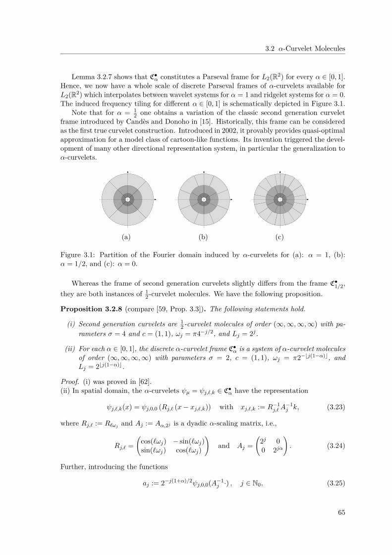
3.2 α-Curvelet Molecules
Lemma 3.2.7 shows that C•α constitutes a Parseval frame for L2(R2) for every α ∈ [0, 1].
Hence, we now have a whole scale of discrete Parseval frames of α-curvelets available forL2(R2) which interpolates between wavelet systems for α = 1 and ridgelet systems for α = 0.The induced frequency tiling for different α ∈ [0, 1] is schematically depicted in Figure 3.1.
Note that for α = 12 one obtains a variation of the classic second generation curvelet
frame introduced by Candès and Donoho in [15]. Historically, this frame can be consideredas the first true curvelet construction. Introduced in 2002, it provably provides quasi-optimalapproximation for a model class of cartoon-like functions. Its invention triggered the devel-opment of many other directional representation system, in particular the generalization toα-curvelets.
(a) (b) (c)
Figure 3.1: Partition of the Fourier domain induced by α-curvelets for (a): α = 1, (b):α = 1/2, and (c): α = 0.
Whereas the frame of second generation curvelets slightly differs from the frame C•1/2,
they are both instances of 12 -curvelet molecules. We have the following proposition.
Proposition 3.2.8 (compare [59, Prop. 3.3]). The following statements hold.
(i) Second generation curvelets are 12 -curvelet molecules of order (∞,∞,∞,∞) with pa-
rameters σ = 4 and c = (1, 1), ωj = π4−j/2, and Lj = 2j.
(ii) For each α ∈ [0, 1], the discrete α-curvelet frame C•α is a system of α-curvelet molecules
of order (∞,∞,∞,∞) with parameters σ = 2, c = (1, 1), ωj = π2−⌊j(1−α)⌋, andLj = 2⌊j(1−α)⌋.
Proof. (i) was proved in [62].(ii) In spatial domain, the α-curvelets ψµ = ψj,ℓ,k ∈ C•
α have the representation
ψj,ℓ,k(x) = ψj,0,0 (Rj,ℓ (x− xj,ℓ,k)) with xj,ℓ,k := R−1j,ℓA
−1j k, (3.23)
where Rj,ℓ := Rℓωjand Aj := Aα,2j is a dyadic α-scaling matrix, i.e.,
Rj,ℓ =
cos(ℓωj) − sin(ℓωj)sin(ℓωj) cos(ℓωj)
and Aj =
2j 00 2jα
. (3.24)
Further, introducing the functions
aj := 2−j(1+α)/2ψj,0,0(A−1j ·) , j ∈ N0, (3.25)
65
3 EXAMPLES OF α-MOLECULES IN L2(R2)
we can write ψj,ℓ,k in the form
ψj,ℓ,k(x) = 2j(1+α)/2aj (AjRj,ℓ (x− xj,ℓ,k)) = 2j(1+α)/2aj (AjRj,ℓx− k) . (3.26)
On the Fourier side the functions (3.25) have the form
aj = 2j(1+α)/2 ψj,0,0(Aj ·) = Wj,0(Aj ·).
Since suppWj,0 ⊆ W+j,0[1/6π] (see (3.19)) and
W+j,0[1/6π] ⊆ [−2j−1, 2j−1] × [−2jα−1, 2jα−1] = Ξj,0,
this implies
supp aj ⊆ [−2−1, 2−1] × [−2−1, 2−1] = Ξ0,0. (3.27)
Further, if j > 0 the function ψj,0,0 vanishes on the square [−2j−7, 2j−7]2. Consequently,the associated function aj vanishes on [−2−7, 2−7] ×
2j(1−α) · [−2−7, 2−7]
.
Next, we analyze the derivatives of aj . First observe that for fixed ρ = (ρ1, ρ2) ∈ N20 the
mixed derivatives ∂ρ11 ∂ρ2
2 Wj,0 obey uniformly in j ∈ N0
∥∂ρ11 ∂ρ2
2 Wj,0∥∞ . 2−jρ12−jαρ2 .
With the chain rule we deduce
∥∂ρaj∥∞ = ∥∂ρ11 ∂ρ2
2 Wj,0(Aj ·)∥∞ = 2jρ12jαρ2∥∂ρ1
1 ∂ρ22 Wj,0
(Aj ·)∥∞ . 1.
Due to supp ∂ρaj ⊆ supp aj , this estimate together with the support properties of aj im-plies (2.5).
As a consequence of this proposition, the α-curvelet frame C•α is in particular a system of
α-molecules of order (∞,∞,∞,∞). Its parametrization (M,ΦM ) consists of the α-curveletindex set M = J × Z2 and the parametrization map ΦM from M into the phase-spaceP = R2 × T × R+ which is given as follows
ΦM : M → P , (j, ℓ, k) →→ (xj,ℓ,k, ℓωj , 2−j) = (R−1ℓωjA−1
j k, ℓωj , 2−j). (3.28)
The frame C•α is a suitable anchor system for the application of the transfer principle for-
mulated in Theorem 2.3.6. It will be used in Chapters 5 and 6 to study cartoon approxima-tion properties of α-molecules. Via the transfer principle, the results obtained for C•
α haveconsequences for many other α-molecule systems. Among these are α-curvelet construc-tions [15, 60], but also band-limited [81, 66, 70] as well as compactly supported [76, 73, 83]α-shearlet systems. A general framework for discrete α-shearlet systems is the topic of thenext section.
66
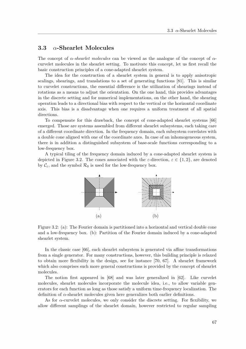
3.3 α-Shearlet Molecules
3.3 α-Shearlet Molecules
The concept of α-shearlet molecules can be viewed as the analogue of the concept of α-curvelet molecules in the shearlet setting. To motivate this concept, let us first recall thebasic construction principles of a cone-adapted shearlet system.
The idea for the construction of a shearlet system in general is to apply anisotropicscalings, shearings, and translations to a set of generating functions [81]. This is similarto curvelet constructions, the essential difference is the utilization of shearings instead ofrotations as a means to adjust the orientation. On the one hand, this provides advantagesin the discrete setting and for numerical implementations, on the other hand, the shearingoperation leads to a directional bias with respect to the vertical or the horizontal coordinateaxis. This bias is a disadvantage when one requires a uniform treatment of all spatialdirections.
To compensate for this drawback, the concept of cone-adapted shearlet systems [66]emerged. Those are systems assembled from different shearlet subsystems, each taking careof a different coordinate direction. In the frequency domain, each subsystem correlates witha double cone aligned with one of the coordinate axes. In case of an inhomogeneous system,there is in addition a distinguished subsystem of base-scale functions corresponding to alow-frequency box.
A typical tiling of the frequency domain induced by a cone-adapted shearlet system isdepicted in Figure 3.2. The cones associated with the ε-direction, ε ∈ 1, 2, are denotedby Cε, and the symbol R0 is used for the low-frequency box.
(a) (b)
Figure 3.2: (a): The Fourier domain is partitioned into a horizontal and vertical double coneand a low-frequency box. (b): Partition of the Fourier domain induced by a cone-adaptedshearlet system.
In the classic case [66], each shearlet subsystem is generated via affine transformationsfrom a single generator. For many constructions, however, this building principle is relaxedto obtain more flexibility in the design, see for instance [70, 67]. A shearlet frameworkwhich also comprises such more general constructions is provided by the concept of shearletmolecules.
The notion first appeared in [68] and was later generalized in [62]. Like curveletmolecules, shearlet molecules incorporate the molecule idea, i.e., to allow variable gen-erators for each function as long as those satisfy a uniform time-frequency localization. Thedefinition of α-shearlet molecules given here generalizes both earlier definitions.
As for α-curvelet molecules, we only consider the discrete setting. For flexibility, weallow different samplings of the shearlet domain, however restricted to regular sampling
67
3 EXAMPLES OF α-MOLECULES IN L2(R2)
grids. Those are specified by a set of parameters, similar to (3.11), namely
σ > 1 , c = (c1, c2) ∈ R2+ , (υj)j∈N0 ∈ RN0
+ with υj ≍ σ−j(1−α). (3.29)
The parameters σ and c determine the scale and translational resolution of the sampling.The numbers υj determine the resolution of the shear sampling.
The subsystems associated to the ε-direction, ε ∈ 1, 2, are indexed by a set Λsε of the
form
Λsε :=
(ε, j, ℓ, k) : j ∈ N0, ℓ ∈ Lε
j , k ∈ Z2, (3.30)
where j ∈ N0 corresponds to the scale, ℓ ∈ Lεj to the orientation, and k ∈ Z2 to the spatial
position of the elements. The possible shears at each scale j are restricted by a nonemptyset
Lεj ⊂ Z such that max
|ℓ| : ℓ ∈ Lε
j
≤ Lε
j ,
where (Lεj)j∈N0 is a sequence of nonnegative integers with Lε
j . σj(1−α).For the subsequent definitions we need the following matrices, where the different ver-
sions correspond to different regions of the frequency domain, i.e., either the cones Cε,ε ∈ 1, 2, or the low-frequency box R0. For the scaling we utilize the α-scaling matrices
A(0)α,t := A
(1)α,t :=
t 00 tα
and A
(2)α,t =
tα 00 t
, t > 0,
for the shearing we utilize the shear matrices
S(0)υ := S(1)
υ :=
1 υ0 1
and S(2)
υ =
1 0υ 1
, υ ∈ R.
Further, the translational grid is obtained from Z2 using matrices of the form
M (0)c := M (1)
c :=c1 00 c2
, M (2)
c =c2 00 c1
, c = (c1, c2) ∈ R2
+.
Now we are ready to introduce the subsystems Msα,ε corresponding to the frequency
cones Cε in ε-direction, ε ∈ 1, 2.
Definition 3.3.1. Let α ∈ [0, 1], ε ∈ 1, 2, and L,M,N1, N2 ∈ N0 ∪ ∞. Further, let thesampling parameters (3.29) be fixed, and let Λs
ε be an index set of the form (3.30). We calla system
Msα,ε :=
mλ ∈ L2(R2) : λ ∈ Λs
ε
a system of α-shearlet molecules of order (L,M,N1, N2) associated with the ε-direction ifthe functions mλ = mε,j,ℓ,k can be represented in the form
mε,j,ℓ,k(·) := σj(1+α)/2γε,j,ℓ,k
A
(ε)α,σjS
(ε)ℓυj
· −M (ε)c k
with generators γε,j,ℓ,k ∈ L2(R2) which satisfy for every ρ ∈ N2
0 with |ρ| ≤ L,
|∂ργε,j,ℓ,k(ξ1, ξ2)| . min
1, σ−j + |ξε| + σ−j(1−α)|ξ3−ε|M
· ⟨|ξ|⟩−N1 · ⟨ξ3−ε⟩−N2 . (3.31)
68
3.3 α-Shearlet Molecules
Hereby the implicit constant shall be independent of the indices (ε, j, ℓ, k) ∈ Λsε and ξ =
(ξ1, ξ2) ∈ R2. The value ∞ of a control parameter indicates that the respective quantitycan be chosen arbitrarily large.
Next, we introduce the system Msα,0 corresponding to the low-frequency box R0. As
index set we use
Λs0 :=
(0, 0, 0, k) : k ∈ Z2
. (3.32)
Definition 3.3.2. Let α ∈ [0, 1] and L,N1, N2 ∈ N0 ∪ ∞. The system Msα,0 of base-scale
functions of order (L,N1, N2) is given by
Msα,0 :=
mλ : λ ∈ Λs
0
with functions mλ ∈ L2(R2) of the form
mλ(·) := γλ(· −M (0)c k) for λ = (0, 0, 0, k) ∈ Λs
0.
The generators γλ ∈ L2(R2) are assumed to satisfy
|∂ργλ(ξ1, ξ2)| . ⟨|ξ|⟩−N1 · ⟨ξ2⟩−N2 , ξ = (ξ1, ξ2) ∈ R2,
for every ρ ∈ N20 with |ρ| ≤ L and with an implicit constant independent of the index λ ∈ Λs
0and ξ = (ξ1, ξ2) ∈ R2.
A full system of α-shearlet molecules for L2(R2) is obtained by combining the systemsMs
α,ε, ε ∈ 0, 1, 2.
Definition 3.3.3. An α-shearlet index set Λs is defined as the union
Λs :=
ε∈0,1,2Λs
ε (3.33)
of sets Λsε of the form (3.30) and (3.32). A system Ms
α := mλ ∈ L2(R2) : λ ∈ Λs,indexed by an α-shearlet index set Λs, constitutes a system of α-shearlet molecules of order(L,M,N1, N2) if the subsystems Ms
α,ε := mλ : λ ∈ Λsε, ε ∈ 1, 2, are systems of α-
shearlet molecules of order (L,M,N1, N2) in the sense of Definition 3.3.1 and if Msα,0 :=
mλ : λ ∈ Λs0 is a system of base-scale functions of order (L,N1, N2) as in Definition 3.3.2.
For convenience, we write this as
Msα =
ε∈0,1,2
Msα,ε.
The definition of α-shearlet molecules is compatible with other notions of shearletmolecules, in particular those defined in [68, Def. 4.1].
Proposition 3.3.4 (compare [62, Prop. 3.14]). Shearlet molecules of regularity R ∈ N0, asdefined in [68], are 1
2 -shearlet molecules of order (∞,∞, R/2, R/2).
Proof. An argument can be found right before [62, Prop. 3.14].
Next we will prove that, like α-curvelet molecules, systems of α-shearlet molecules con-stitute their own subclass of discrete α-molecule systems.
69
3 EXAMPLES OF α-MOLECULES IN L2(R2)
3.3.1 The α-Shearlet Parametrization
Since the construction of α-shearlet molecules is based on shearings instead of rotations, theassociated parametrizations need to adequately translate the shearing parameters to corre-sponding orientation angles. This complicates their definition compared to the definition ofthe α-curvelet parametrizations in Definition 3.2.3.
Definition 3.3.5. With parameters given as in (3.29), an α-shearlet parametrization (Λs,Φs)consists of an index set Λs of the form (3.33) and a map Φs : Λs → P from Λs intoP = R2 × T × R+ defined by
Φs : (ε, j, ℓ, k) →→S
(ε)−ℓυj
A(ε)α,σ−jM
(ε)c k,
max0, ε− 1π/2 + arctan(−ℓυj)
2π, σ−j
.
Now we are ready to prove the essential result that α-shearlet molecules are instancesof α-molecules. In fact, they can even be characterized as precisely those systems of α-molecules which correspond to an α-shearlet parametrization.
Proposition 3.3.6 (compare [59, Prop. 3.9]). Every system of α-shearlet molecules oforder (L,M,N1, N2) constitutes a system of α-molecules of the same order with respect toa corresponding α-shearlet parametrization, and vice versa.
Proof. The main ingredients of the proof can be found in [59, Subsec. 6.1.1], where [59,Prop. 3.9] is proved.
Let Msα := mλλ∈Λs be a function system in L2(R2) indexed by a set Λs = Λs
0 ∪Λs1 ∪Λs
2of the form (3.33). Further, let Φs : λ →→ (xλ, ηλ, tλ) denote an α-shearlet parametrizationsubject to parameters σ, c = (c1, c2), (υj)j∈N0 as in (3.29).
Clearly, for each λ ∈ Λs there exist unique functions gλ, γλ ∈ L2(R2) such that
t−(1+α)/2λ γλ
A
(ε)α,t−1
λ
S(ε)υλ
· −M (ε)c k
= mλ = t
−(1+α)/2λ gλ
A−1
α,tλRηλ
(· − xλ),
where υλ := ℓυj . We need to show that the Fourier transform gλ of gλ satisfies (2.5) if andonly if γλ satisfies (3.31). For this investigation we decompose
Msα =
ε∈0,1,2
Msα,ε
and handle the subsystems Msα,ε := mλλ∈Λs
ε, ε ∈ 0, 1, 2, separately.
Let us begin with the case ε = 0. Then gλ = γλ and the assertion is obvious.Of the cases ε ∈ 1, 2, we only handle ε = 1 since the arguments for the case ε = 2 areessentially the same. For Ms
α,1 the relation between gλ and γλ can be expressed by
γλ(·) = gλ
Tj,ℓ ·
and gλ(·) = γλ
T−1
j,ℓ ·
(3.34)
with a matrix
Tj,ℓ := A−1α,tλ
RηλS−1
ℓυjAα,tλ
, (3.35)
which describes the transfer from the rotation-based to the shear-based generators. Let usinvestigate the properties of this ‘transfer matrix’ Tj,ℓ.
70
3.3 α-Shearlet Molecules
For this purpose, it is useful to first examine the matrix Tj,ℓ := RηλS−1
ℓυj. Since ηλ =
(arctan(−ℓυj))2π, we have
Sℓυj=
1 ℓυj
0 1
=
1 − tan(ηλ)0 1
.
Using
0 = tan(ηλ) cos(ηλ) − sin(ηλ) and cos(ηλ)−1 = tan(ηλ) sin(ηλ) + cos(ηλ),
we calculate
Tj,ℓ =
cos(ηλ) 0sin(ηλ) cos(ηλ)−1
=
1√1+(ℓυj)2 0−ℓυj√
1+(ℓυj)2
1 + (ℓυj)2
=:a(j, ℓ) 0b(j, ℓ) c(j, ℓ)
.
Taking into account a(j, ℓ) = c(j, ℓ)−1, we obtain for the inverse
T−1j,ℓ =
c(j, ℓ) 0
−b(j, ℓ) a(j, ℓ)
=
1 + (ℓυj)2 0ℓυj√
1+(ℓυj)21√
1+(ℓυj)2
.By assumption |ℓ| . σj(1−α) and υj ≍ σ−j(1−α), which implies the existence of a bound
B > 0 such that
|ℓυj | ≤ B for all j ∈ N0, ℓ ∈ L1j .
Hence, uniformly for all j ∈ N0 and ℓ ∈ L1j
1/
1 +B2 ≤ a(j, ℓ) ≤ 1 ≤ c(j, ℓ) ≤
1 +B2 , |b(j, ℓ)| ≤ B/
1 +B2. (3.36)
Turning to the matrix Tj,ℓ, we calculate
Tj,ℓ =
a(j, ℓ) 0σ−j(1−α)b(j, ℓ) c(j, ℓ)
and T−1
j,ℓ =
c(j, ℓ) 0−σ−j(1−α)b(j, ℓ) a(j, ℓ)
.
Since |σ−j(1−α)| ≤ 1 for every j ∈ N0, we obtain for the Frobenius norm
∥T Tj,ℓ∥F = ∥Tj,ℓ∥F ≤
2 +B2 and ∥T−T
j,ℓ ∥F = ∥T−1j,ℓ ∥F ≤
2 +B2.
As a consequence, we have uniformly in j ∈ N0, ℓ ∈ L1j ,
1√2 +B2
|ξ| ≤ |T Tj,ℓξ| ≤
2 +B2|ξ| for all ξ ∈ R2 , (3.37)
and the respective relation for |T−Tj,ℓ ξ|. Since detTj,ℓ = detT−1
j,ℓ = 1, we obtain from (3.34)
γλ(·) = gλ
T−T
j,ℓ ·
and gλ(·) = γλ
T T
j,ℓ ·.
71
3 EXAMPLES OF α-MOLECULES IN L2(R2)
Now we are ready to show that the assumption (3.31) on γλ implies property (2.5) for gλ,and vice versa. Using |σ−j(1−α)| ≤ 1, the uniform boundedness of |a(j, ℓ)|, |b(j, ℓ)|, |c(j, ℓ)|,and the chain rule, we can estimate for any ρ ∈ N2
0 with |ρ| ≤ L,
|∂ρgλ(ξ)| . sup|ν|≤L
∂ν γλ
a(j, ℓ) σ−j(1−α)b(j, ℓ)
0 c(j, ℓ)
ξ
. (3.38)
Utilizing the moment estimate in (3.31) for γλ gives the moment property required in (2.5),namely
|∂ρgλ(ξ)| .σ−j + |a(j, ℓ)ξ1 + σ−j(1−α)b(j, ℓ)ξ2| + σ−j(1−α)|c(j, ℓ)ξ2|
M
.tλ + |ξ1| + t1−α
λ |ξ2|M
.
It remains to show the decay of ∂ρgλ for large frequencies ξ = (ξ1, ξ2) ∈ R2. We obtainfrom (3.38) and the decay estimate in (3.31),
|∂ρgλ(ξ)| .a(j, ℓ) σ−j(1−α)b(j, ℓ)
0 c(j, ℓ)
ξ
−N1
⟨c(j, ℓ)ξ2⟩−N2 . ⟨|ξ|⟩−N1 ⟨ξ2⟩−N2 ,
where the last estimate is a consequence of |T Tj,ℓξ| ≍ |ξ| due to (3.37) and c(j, ℓ)ξ2 ≍ ξ2.
We finish the proof by noting that an analogous argumentation, with the matrix T−Tj,ℓ
taking the role of T Tj,ℓ, yields (3.31) for γλ under the assumption (2.5) on gλ.
3.3.2 A Sufficient Frame Condition for α-Shearlet Molecules
We will now use Theorem 2.4.1 to derive a sufficient frame criterion for α-shearlet moleculessimilar to Theorem 3.2.5. First, recall that an α-shearlet parametrization (Λs,Φs) is deter-mined by an α-shearlet index set, which can be decomposed in the form
Λs = ∆s × Z2 with ∆s :=
(0, 0, 0)
∪
(ε, j, ℓ) : ε ∈ 1, 2, j ∈ N0, ℓ ∈ Lεj
,
and a corresponding parametrization map
Φs : Λs → P : (ε, j, ℓ, k) →→S
(ε)−ℓυj
A(ε)α,σ−jM
(ε)c k,
max0, ε− 1π2 + arctan(−ℓυj)
2π, σ−j
.
Hence, α-shearlet parametrizations have the structure (2.34) if for each µ = (ε, j, ℓ) ∈ ∆s
we choose Tµ := T(ε)j,ℓ M
(ε)c M−1
c with the matrix
T(ε)j,ℓ := A−1
α,tµRηµS
(ε)−ℓυj
A(ε)α,tµ
. (3.39)
Note that indeed | det(Tµ)| = 1, as required. Note further that the matrices T (ε)j,ℓ are transfer
matrices of the type (3.35) which were analyzed in the proof of Proposition 3.3.6.Now let mλλ∈Λs be a system of α-shearlet molecules with associated shear-based
generators γλλ∈Λs and assume that the functions γλ = γµ,k do not depend on k ∈ Z2.In this situation the frame criterion for α-molecules, Theorem 2.4.1, can be applied topositively decide whether this system forms a frame for L2(R2).
72
3.3 α-Shearlet Molecules
In the case of α-shearlet molecules, it is more convenient to formulate the correlationfunctions in terms of the shear-based generators γλ = γµ, λ = (µ, k) ∈ Λs. Hence, weintroduce the functions Φs : R2 × R2 → R and Γs : R2 → R as
Φs(ξ, ω) :=
µ∈∆s
|γµ(A(ε)α,tµ
(S(ε)ℓυj
)−T ξ)||γµ(A(ε)α,tµ
(S(ε)ℓυj
)−T ξ + (M (ε)c )−1Mcω)|,
Γs(ω) := ess supξ∈R2
Φs(ξ, ω).(3.40)
For c = (c1, c2) ∈ R2+, we further define
Rs(c) :=
m∈Z2\0
Γs(M−1
c m)Γs(−M−1c m)
1/2.
Then we have the following result.
Theorem 3.3.7. Let mλλ∈Λs be a system of α-shearlet molecules with a correspondingfamily of generators γλλ∈Λs, and assume that the generators γλ = γµ,k do not vary withk ∈ Z2. Further, let c = (c1, c2) ∈ R2
+ be the parameter in (3.29) associated with the densityof the translation grid. Then the condition
Rs(c) < Lsinf ≤ Ls
sup < ∞
for the quantities
Lsinf := ess inf
ξ∈R2Φs(ξ, 0) and Ls
sup := Γs(0) = ess supξ∈R2
Φs(ξ, 0)
ensures that mλλ∈Λs constitutes a frame for L2(R2) with frame bounds A,B > 0 satisfying
Lsinf −Rs(c)| detMc|
≤ A ≤ B ≤Ls
sup +Rs(c)| detMc|
.
Proof. The system mλλ∈Λs is a system of α-molecules with respect to an α-shearletparametrization. The associated rotation-based generators are given by gµ = γµ((T (ε)
j,ℓ )−1·),where T (ε)
j,ℓ is the transfer matrix (3.39). It follows
γµ = gµ((T (ε)j,ℓ )−T ·) = gµ(Aα,tµRηµ(S(ε)
ℓυj)T (A(ε)
α,tµ)−1·).
Plugging this into (3.40) yields for the correlation function
Φs(ξ, ω) =
µ∈∆s
|gµ(Aα,tµRηµξ)||gµ(Aα,tµRηµξ + T−Tµ ω)|,
where T−Tµ = (T (ε)
j,ℓ )−T (M (ε)c )−1Mc. Hence we can apply Theorem 2.4.1 and the assertion
follows.
Finally note that SℓAα,σj = Aα,σjSℓυjif υj = σ−j(1−α). Hence for a strict α-shearlet
system as in Definition 3.3.8 this is precisely the criterion proved in [76, Thm. 3.4].
73
3 EXAMPLES OF α-MOLECULES IN L2(R2)
3.3.3 Discrete α-Shearlet Systems
The concept of α-shearlet molecules comprises many common cone-adapted shearlet con-structions. These include band-limited as well as compactly supported systems, as we willsee below.
The general structure of a regular cone-adapted discrete α-shearlet system is recalled inDefinition 3.3.8. It is a generalization of [80, Def. 11] to α-scaling. Note, that sometimesthe parameter β = α−1 is used in the definition instead, as for example in [59, Def. 3.10].
Definition 3.3.8 (compare [59, Def. 3.10]). For c = (c1, c2) ∈ R2+ and α ∈ (0, 1), the
cone-adapted α-shearlet system SHφ, ψ, ψ; c, α
generated by φ, ψ, ψ ∈ L2(R2) is defined
bySH
φ, ψ, ψ; c, α
:= Φ(φ; c, α) ∪ Ψ(ψ; c, α) ∪ Ψ(ψ; c, α),
where, with β = α−1,
Φ(φ; c, α) := φk = φ(· −M (0)c k) : k ∈ Z2,
Ψ(ψ; c, α) :=ψj,ℓ,k = 2j(β+1)/4ψ(S(1)
ℓ A(1)α,2jβ/2 · −M (1)
c k) : j ∈ N0, |ℓ| ≤ ⌈2j(β−1)/2⌉, k ∈ Z2,Ψ(ψ; c, α) :=
ψj,ℓ,k = 2j(β+1)/4ψ(S(2)
ℓ A(2)α,2jβ/2 · −M (2)
c k) : j ∈ N0, |ℓ| ≤ ⌈2j(β−1)/2⌉, k ∈ Z2.In the following, we present some examples of cone-adapted α-shearlet systems as in
Definition 3.3.8. Thereby the generators φ, ψ, ψ ∈ L2(R2) are assumed to be either band-limited or compactly supported.
In the band-limited case, we require φ, ψ, ˆψ ∈ C∞0 (R2) and a frequency support of the
formsupp φ ⊆ Q, supp ψ ⊆ W, supp ˆψ ⊆ W ,
with Q ⊂ R2 being a cube centered at the origin and W, W ⊂ R2 being sets of the form
W = [−a, a] × ([−c,−b] ∪ [b, c]), W = ([−c,−b] ∪ [b, c]) × [−a, a]
with 0 < b < c and 0 < a.In the compact case, the coarse-scale generator φ shall satisfy
φ ∈ CN1+N20 (R2).
Furthermore, we assume the separability of ψ ∈ L2(R2), i.e. ψ(x1, x2) = ψ1(x1)ψ2(x2), andlet ψ be its rotation by π/2. Finally, the functions ψ1, ψ2 shall satisfy
ψ1 ∈ CN10 (R) and ψ2 ∈ CN1+N2
0 (R),
and for ψ1 we assume M ∈ N0 vanishing moments.The following proposition shows that under these assumptions the systems SH
φ, ψ, ψ; c, α
are instances of α-shearlet molecules.
Proposition 3.3.9 ([59, Prop. 3.11]). Let α ∈ (0, 1), β = α−1, and c ∈ R2+ be fixed
parameters. The following statements hold.
(i) For band-limited generators φ, ψ, and ψ subject to the conditions above, the cone-adapted α-shearlet system SH
φ, ψ, ψ; c, α
is a system of α-shearlet molecules of order
(∞,∞,∞,∞) with σ = 2β/2, υj = σ−j(1−α), and Lj = ⌈σj(1−α)⌉.
74
3.3 α-Shearlet Molecules
(ii) For compactly supported generators φ, ψ, and ψ subject to the conditions above, thecone-adapted α-shearlet system SH
φ, ψ, ψ; c, α
is a system of α-shearlet molecules
of order (L,M − L,N1, N2), where L ∈ 0, . . . ,M is arbitrary, with σ = 2β/2, υj =σ−j(1−α), and Lj = ⌈σj(1−α)⌉.
Proof. For the proof we also refer to [59, Subsec. 6.1.2].Let us first rename the functions of the system SH(φ, ψ, ψ; c, α). For j ∈ N0, ℓ ∈ Z with
|ℓ| ≤ ⌈2j(β−1)/2⌉, and k ∈ Z2 we put
ψ0,0,0,k := φk = φ(· −M (0)c k),
ψ1,j,ℓ,k := ψj,ℓ,k = 2j(β+1)/4ψ(S(1)ℓ A
(1)α,2jβ/2 · −M (1)
c k),
ψ2,j,ℓ,k := ψj,ℓ,k = 2j(β+1)/4ψ(S(2)ℓ A
(2)α,2jβ/2 · −M (2)
c k).
With σ = 2β/2 we can rewrite A(1)α,2jβ/2 = A
(1)α,σj and A
(2)α,2jβ/2 = A
(2)α,σj . Further, using
υj = σ−j(1−α), we obtain
S(1)ℓ A
(1)α,σj = A
(1)α,σjS
(1)ℓσ−j(1−α) = A
(1)α,σjS
(1)ℓυj
andS
(2)ℓ A
(2)α,σj = A
(2)α,σjS
(2)ℓσ−j(1−α) = A
(2)α,σjS
(2)ℓυj.
Finally, due to 2j(β+1)/4 = σj(1+α)/2, we arrive at the representation
ψ0,0,0,k = φ(· −M (0)c k),
ψ1,j,ℓ,k = σj(1+α)/2ψ(A(1)α,σjS
(1)ℓυj
· −M (1)c k),
ψ2,j,ℓ,k = σj(1+α)/2ψ(A(2)α,σjS
(2)ℓυj
· −M (2)c k).
Hence, the system SH(φ, ψ, ψ; c, α) = ψλλ∈Λs has the structure of a system of α-shearletmolecules generated by γ1,j,ℓ,k := ψ, γ2,j,ℓ,k := ψ, and γ0,0,0,k := φ.
It remains to prove that these generators satisfy (3.31). In case of band-limited functionsthe proof is analogous to the proof of Proposition 3.2.8(ii). The only interesting part is thusthe case of generators with compact support. Here we restrict our considerations to thefunctions γ1,j,ℓ,k = ψ.
The inverse Fourier transform of ∂ρψ, where ρ ∈ N20, is up to a constant given by
x →→ xρψ(x). By smoothness and compact support of ψ1, ψ2, we find that for any |ρ| ≤ Lthe functions
x →→ ∂(N1,N1+N2)xρψ(x)
and x →→ xρψ(x)
belong to L1(R2). Hence, on the Fourier side
ξ →→ ξN11 ξN1+N2
2 ∂ρψ(ξ) and ξ →→ ∂ρψ(ξ)
are continuous and contained in L∞(R2). It follows that
⟨ξ1⟩N1⟨ξ2⟩N1+N2∂ρψ(ξ)
75
3 EXAMPLES OF α-MOLECULES IN L2(R2)
is bounded in modulus. Using ⟨x⟩⟨y⟩ ≥ ⟨x2 + y2⟩ we get the decay estimate for large
frequencies|∂ρψ(ξ)| . ⟨|ξ|⟩−N1⟨ξ2⟩−N2 .
Let us turn to the moment conditions. Let ρ = (ρ1, ρ2) ∈ N20 with |ρ1| ≤ L for some
L = 0, . . . ,M . Thenxρψ(x) = xρ1
1 ψ1(x1)xρ22 ψ2(x2)
restricted to the variable x1 possesses at least M−L vanishing moments, since ψ1 is assumedto possess M vanishing moments. This yields a decay of order min1, |ξ1|M−L for thederivatives up to order L of ψ by the following lemma, whose proof can be found, e.g., in[62].
Lemma 3.3.10 ([62]). Suppose that g : R → C is continuous, compactly supported andpossesses M vanishing moments. Then
|g(ξ)| . min1, |ξ|M .
The proof is finished.
Proposition 3.3.9 shows that various versions of cone-adapted shearlet systems are unitedunder the roof of α-shearlet molecules. Furthermore, also non-affine constructions such asthe smooth Parseval frame of shearlets by Guo and Labate [70, 67] fall into this generalframework.
Since, by Proposition 3.3.6, α-shearlet molecules are particular instances of α-molecules,these examples further show that the concept of α-molecules is general enough to includeboth shear-based and rotation-based constructions.
3.4 Consistency of α-Curvelet and α-Shearlet Parametriza-tions
Despite their different constructions, shearlet and curvelet systems are closely related andin many respects exhibit a similar behavior. For example, the same approximation rateswith respect to cartoon-like data have been observed for various systems [15, 60, 67, 78, 73].An explanation for this similar behavior can be given by the framework of α-molecules.
Both, α-curvelets and α-shearlets are instances of discrete α-molecule systems and, aswe will prove in this section, the corresponding parametrizations are consistent in the senseof Definition 2.3.5. Hence, the same approximation rates are a direct consequence of thetransfer principle for α-molecules, Theorem 2.3.6.
In the main result of this section, Theorem 3.4.3, we first compare the α-curvelet andα-shearlet parametrizations with the canonical parametrization from Definition 3.1.2. As acorollary, we can then easily deduce the consistency of the different α-curvelet and α-shearletparametrizations among themselves, stated in Corollary 3.4.4.
For the proof of Theorem 3.4.3, we need two auxiliary lemmas. The first one is givenbelow.
Lemma 3.4.1. Let 0 ≤ δ < π2 be fixed. Then uniformly for |η| ≤ δ and |θ| ≤ π
2
|η − θ| ≍ |η − θ|.
76
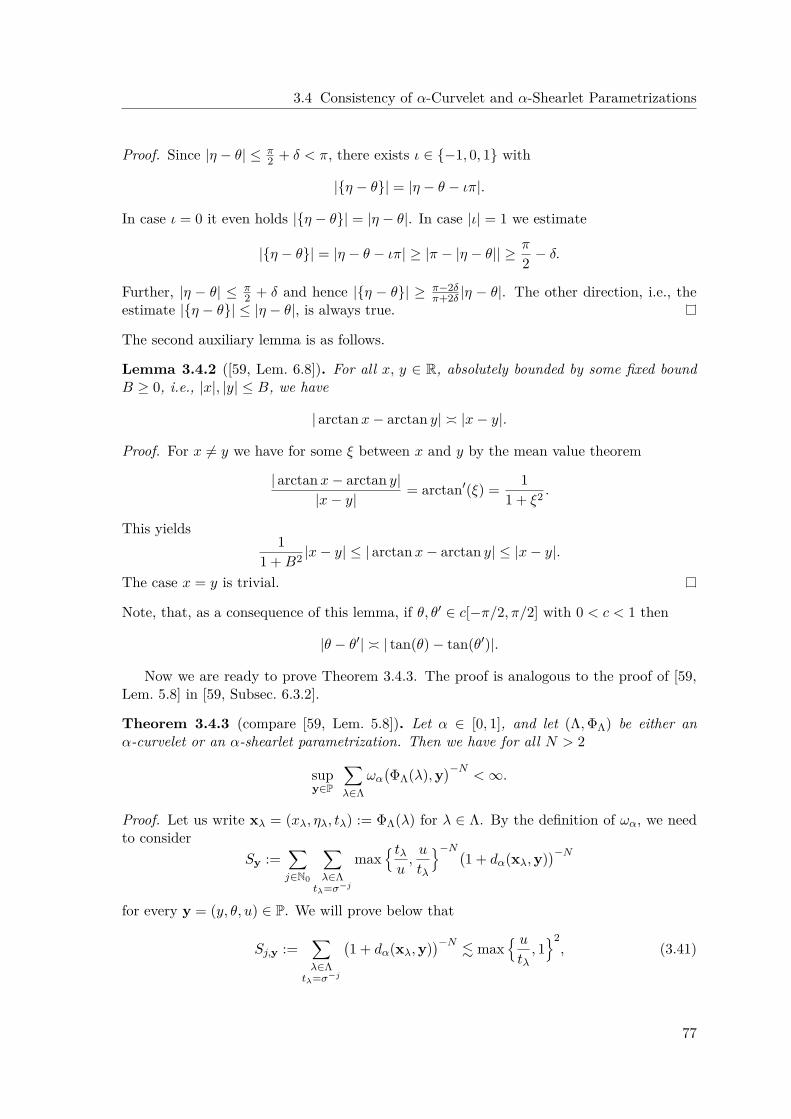
3.4 Consistency of α-Curvelet and α-Shearlet Parametrizations
Proof. Since |η − θ| ≤ π2 + δ < π, there exists ι ∈ −1, 0, 1 with
|η − θ| = |η − θ − ιπ|.
In case ι = 0 it even holds |η − θ| = |η − θ|. In case |ι| = 1 we estimate
|η − θ| = |η − θ − ιπ| ≥ |π − |η − θ|| ≥ π
2 − δ.
Further, |η − θ| ≤ π2 + δ and hence |η − θ| ≥ π−2δ
π+2δ |η − θ|. The other direction, i.e., theestimate |η − θ| ≤ |η − θ|, is always true.
The second auxiliary lemma is as follows.
Lemma 3.4.2 ([59, Lem. 6.8]). For all x, y ∈ R, absolutely bounded by some fixed boundB ≥ 0, i.e., |x|, |y| ≤ B, we have
| arctan x− arctan y| ≍ |x− y|.
Proof. For x = y we have for some ξ between x and y by the mean value theorem
| arctan x− arctan y||x− y|
= arctan′(ξ) = 11 + ξ2 .
This yields1
1 +B2 |x− y| ≤ | arctan x− arctan y| ≤ |x− y|.
The case x = y is trivial.
Note, that, as a consequence of this lemma, if θ, θ′ ∈ c[−π/2, π/2] with 0 < c < 1 then
|θ − θ′| ≍ | tan(θ) − tan(θ′)|.
Now we are ready to prove Theorem 3.4.3. The proof is analogous to the proof of [59,Lem. 5.8] in [59, Subsec. 6.3.2].
Theorem 3.4.3 (compare [59, Lem. 5.8]). Let α ∈ [0, 1], and let (Λ,ΦΛ) be either anα-curvelet or an α-shearlet parametrization. Then we have for all N > 2
supy∈P
λ∈Λ
ωαΦΛ(λ),y
−N< ∞.
Proof. Let us write xλ = (xλ, ηλ, tλ) := ΦΛ(λ) for λ ∈ Λ. By the definition of ωα, we needto consider
Sy :=
j∈N0
λ∈Λ
tλ=σ−j
max tλu,u
tλ
−N1 + dα(xλ,y)
−N
for every y = (y, θ, u) ∈ P. We will prove below that
Sj,y :=λ∈Λ
tλ=σ−j
1 + dα(xλ,y)
−N. max
utλ, 12, (3.41)
77
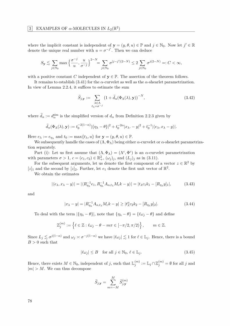
3 EXAMPLES OF α-MOLECULES IN L2(R2)
where the implicit constant is independent of y = (y, θ, u) ∈ P and j ∈ N0. Now let j′ ∈ Rdenote the unique real number with u = σ−j′ . Then we can deduce
Sy .
j∈N0
maxσ−j
u,u
σ−j
2−N=
j∈N0
σ|j−j′|(2−N) ≤ 2
j∈N0
σj(2−N) =: C < ∞,
with a positive constant C independent of y ∈ P. The assertion of the theorem follows.It remains to establish (3.41) for the α-curvelet as well as the α-shearlet parametrization.
In view of Lemma 2.2.4, it suffices to estimate the sum
Sj,y :=λ∈Λ
tλ=σ−j
1 + dα(ΦΛ(λ),y)
−N, (3.42)
where dα := dsimα is the simplified version of dα from Definition 2.2.3 given by
dα(ΦΛ(λ),y) := t−2(1−α)0 |ηλ − θ|2 + t−2α
0 |xλ.− y|2 + t−10 |⟨eλ, xλ − y⟩|.
Here eλ := eηλand t0 := maxtλ, u for y = (y, θ, u) ∈ P.
We subsequently handle the cases of (Λ,ΦΛ) being either α-curvelet or α-shearlet parametriza-tion separately.
Part (i): Let us first assume that (Λ,ΦΛ) = (Λc,Φc) is an α-curvelet parametrizationwith parameters σ > 1, c = (c1, c2) ∈ R2
+, (ωj)j , and (Lj)j as in (3.11).For the subsequent arguments, let us denote the first component of a vector z ∈ R2 by
[z]1 and the second by [z]2. Further, let e1 denote the first unit vector of R2.We obtain the estimates
|⟨eλ, xλ − y⟩| = |⟨R−1ηλe1, R
−1ηλAα,tλ
Mck − y⟩| = |tλc1k1 − [Rηλy]1|, (3.43)
and
|xλ − y| = |R−1ηλAα,tλ
Mck − y| ≥ |tαλc2k2 − [Rηλy]2|. (3.44)
To deal with the term |ηλ − θ|, note that ηλ − θ = ℓωj − θ and define
Z(m)j :=
ℓ ∈ Z : ℓωj − θ −mπ ∈ [−π/2, π/2)
, m ∈ Z.
Since Lj . σj(1−α) and ωj ≍ σ−j(1−α) we have |ℓωj | . 1 for ℓ ∈ Lj . Hence, there is a boundB > 0 such that
|ℓωj | ≤ B for all j ∈ N0, ℓ ∈ Lj . (3.45)
Hence, there exists M ∈ N0, independent of j, such that L(m)j := Lj ∩Z(m)
j = ∅ for all j and|m| > M . We can thus decompose
Sj,y =M
m=−M
S(m)j,y
78
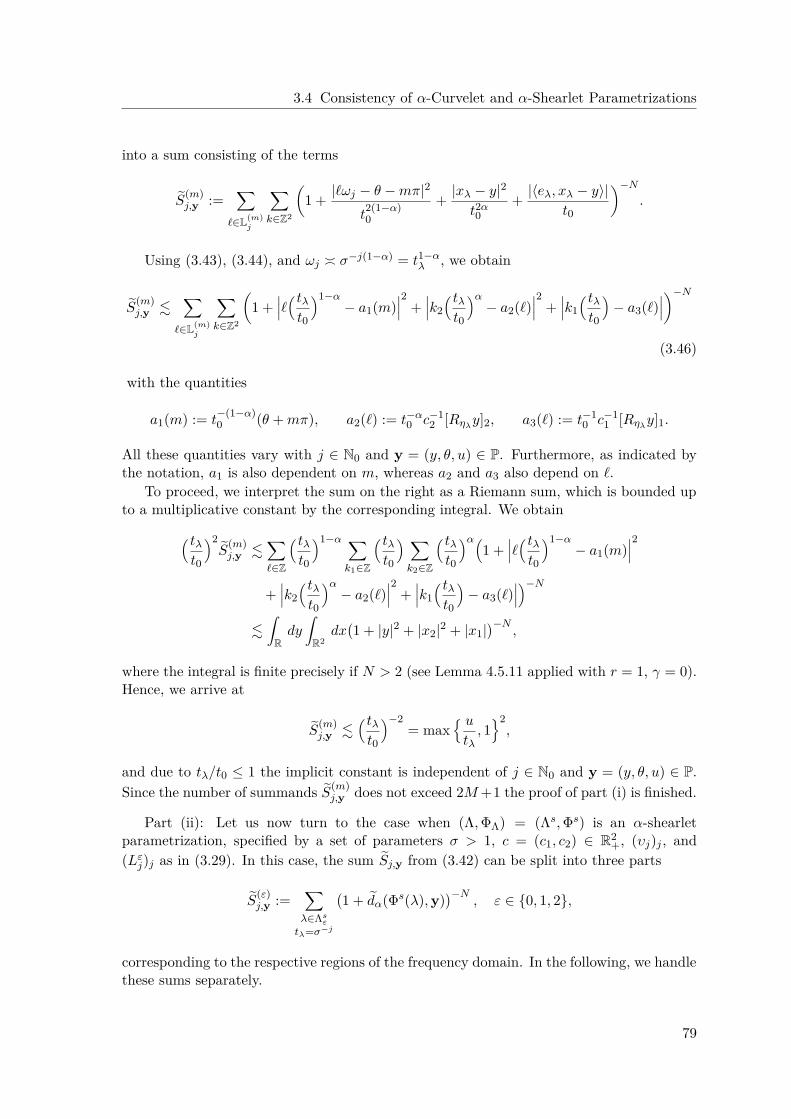
3.4 Consistency of α-Curvelet and α-Shearlet Parametrizations
into a sum consisting of the terms
S(m)j,y :=
ℓ∈L(m)
j
k∈Z2
1 + |ℓωj − θ −mπ|2
t2(1−α)0
+ |xλ − y|2
t2α0
+ |⟨eλ, xλ − y⟩|t0
−N
.
Using (3.43), (3.44), and ωj ≍ σ−j(1−α) = t1−αλ , we obtain
S(m)j,y .
ℓ∈L(m)
j
k∈Z2
1 +
ℓ tλt0
1−α− a1(m)
2 +k2 tλt0
α− a2(ℓ)
2 +k1 tλt0
− a3(ℓ)
−N
(3.46)
with the quantities
a1(m) := t−(1−α)0 (θ +mπ), a2(ℓ) := t−α
0 c−12 [Rηλ
y]2, a3(ℓ) := t−10 c−1
1 [Rηλy]1.
All these quantities vary with j ∈ N0 and y = (y, θ, u) ∈ P. Furthermore, as indicated bythe notation, a1 is also dependent on m, whereas a2 and a3 also depend on ℓ.
To proceed, we interpret the sum on the right as a Riemann sum, which is bounded upto a multiplicative constant by the corresponding integral. We obtain
tλt0
2 S(m)j,y .
ℓ∈Z
tλt0
1−α k1∈Z
tλt0
k2∈Z
tλt0
α1 +
ℓ tλt0
1−α− a1(m)
2+k2 tλt0
α− a2(ℓ)
2 +k1 tλt0
− a3(ℓ)
−N
.Rdy
R2dx1 + |y|2 + |x2|2 + |x1|
−N,
where the integral is finite precisely if N > 2 (see Lemma 4.5.11 applied with r = 1, γ = 0).Hence, we arrive at
S(m)j,y .
tλt0
−2= max
utλ, 12,
and due to tλ/t0 ≤ 1 the implicit constant is independent of j ∈ N0 and y = (y, θ, u) ∈ P.Since the number of summands S(m)
j,y does not exceed 2M+1 the proof of part (i) is finished.
Part (ii): Let us now turn to the case when (Λ,ΦΛ) = (Λs,Φs) is an α-shearletparametrization, specified by a set of parameters σ > 1, c = (c1, c2) ∈ R2
+, (υj)j , and(Lε
j)j as in (3.29). In this case, the sum Sj,y from (3.42) can be split into three parts
S(ε)j,y :=
λ∈Λs
ε
tλ=σ−j
1 + dα(Φs(λ),y)
−N, ε ∈ 0, 1, 2,
corresponding to the respective regions of the frequency domain. In the following, we handlethese sums separately.
79
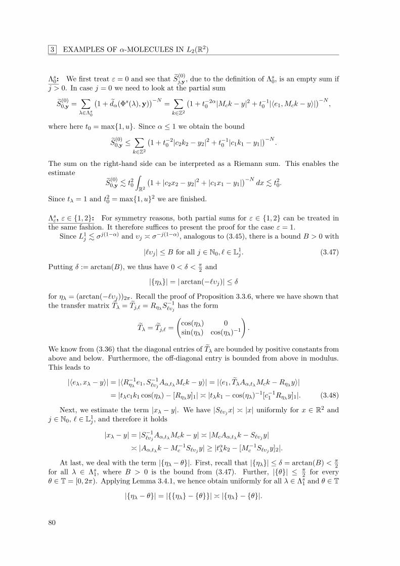
3 EXAMPLES OF α-MOLECULES IN L2(R2)
Λs0: We first treat ε = 0 and see that S(0)
j,y , due to the definition of Λs0, is an empty sum if
j > 0. In case j = 0 we need to look at the partial sum
S(0)0,y =
λ∈Λs
0
1 + dα(Φs(λ),y)
−N =
k∈Z2
1 + t−2α
0 |Mck − y|2 + t−10 |⟨e1,Mck − y⟩|
−N,
where here t0 = max1, u. Since α ≤ 1 we obtain the bound
S(0)0,y ≤
k∈Z2
1 + t−2
0 |c2k2 − y2|2 + t−10 |c1k1 − y1|
−N.
The sum on the right-hand side can be interpreted as a Riemann sum. This enables theestimate S(0)
0,y . t20
R2
1 + |c2x2 − y2|2 + |c1x1 − y1|
−Ndx . t20.
Since tλ = 1 and t20 = max1, u2 we are finished.
Λsε, ε ∈ 1, 2: For symmetry reasons, both partial sums for ε ∈ 1, 2 can be treated in
the same fashion. It therefore suffices to present the proof for the case ε = 1.Since L1
j . σj(1−α) and υj ≍ σ−j(1−α), analogous to (3.45), there is a bound B > 0 with
|ℓυj | ≤ B for all j ∈ N0, ℓ ∈ L1j . (3.47)
Putting δ := arctan(B), we thus have 0 < δ < π2 and
|ηλ| = | arctan(−ℓυj)| ≤ δ
for ηλ = (arctan(−ℓυj))2π. Recall the proof of Proposition 3.3.6, where we have shown thatthe transfer matrix Tλ = Tj,ℓ = Rηλ
S−1ℓυj
has the form
Tλ = Tj,ℓ =
cos(ηλ) 0sin(ηλ) cos(ηλ)−1
.
We know from (3.36) that the diagonal entries of Tλ are bounded by positive constants fromabove and below. Furthermore, the off-diagonal entry is bounded from above in modulus.This leads to
|⟨eλ, xλ − y⟩| = |⟨R−1ηλe1, S
−1ℓυjAα,tλ
Mck − y⟩| = |⟨e1, TλAα,tλMck −Rηλ
y⟩|
= |tλc1k1 cos(ηλ) − [Rηλy]1| ≍ |tλk1 − cos(ηλ)−1[c−1
1 Rηλy]1|. (3.48)
Next, we estimate the term |xλ − y|. We have |Sℓυjx| ≍ |x| uniformly for x ∈ R2 and
j ∈ N0, ℓ ∈ L1j , and therefore it holds
|xλ − y| = |S−1ℓυjAα,tλ
Mck − y| ≍ |McAα,tλk − Sℓυj
y|
≍ |Aα,tλk −M−1
c Sℓυjy| ≥ |tαλk2 − [M−1
c Sℓυjy]2|.
At last, we deal with the term |ηλ − θ|. First, recall that |ηλ| ≤ δ = arctan(B) < π2
for all λ ∈ Λs1, where B > 0 is the bound from (3.47). Further, |θ| ≤ π
2 for everyθ ∈ T = [0, 2π). Applying Lemma 3.4.1, we hence obtain uniformly for all λ ∈ Λs
1 and θ ∈ T
|ηλ − θ| = |ηλ − θ| ≍ |ηλ − θ|.
80
3.5 Wavelet Systems
Next, we distinguish between those θ ∈ T with |θ| ≤ arctan(B + 1) and those with|θ| > arctan(B + 1).
For |θ| ≤ arctan(B + 1), we use Lemma 3.4.2 and tan(θ) = tan(θ) to obtain
|ηλ − θ| ≍ |ηλ − θ| = | arctan(−ℓυj) − θ| ≍ |ℓυj + tan(θ)|.
In case |θ| > arctan(B + 1) we estimate directly, using |ηλ| ≤ arctan(B),
|ηλ − θ| ≍ |ηλ − θ| ≥|ηλ| − |θ|
> arctan(B + 1) − arctan(B) > 0.
Since |ℓυj | ≤ B according to (3.47) this implies |ηλ − θ| & |ℓυj |.We now introduce the quantity
q(θ) :=
tan(θ) , |θ| ≤ arctan(B + 1),0 , |θ| > arctan(B + 1).
Then we can summarize
|ηλ − θ| & |ℓυj + q(θ)|. (3.49)
In view of the estimates (3.48)-(3.49) and υj ≍ σ−j(1−α) ≍ t1−αλ , we obtain
S(1)j,y .
ℓ∈Lj
k∈Z2
1 + |ℓυj + q(θ)|2
t2(1−α)0
+|tαλk2 − [c−1
2 Sℓυjy]2|2
t2α0
+ |tλk1 − [c−11 Rηλ
y]1/ cos(ηλ)|t0
−N
.ℓ∈Z
k∈Z2
1 +
ℓ tλt0
(1−α)− a1(θ)
2 +k2 tλt0
α− a2(ℓ)
2 +k1 tλt0
− a3(ℓ)
−N
with the quantities
a1(θ) := −t−(1−α)0 q(θ), a2(ℓ) := t−α
0 [c−12 Sℓυj
y]2, a3(ℓ) := t−10 [c−1
1 Rηλy]1/ cos(ηλ),
depending on j, ℓ, θ and y. This expression is similar to (3.46). Therefore, from here wecan proceed as in part (i) of the proof.
As a corollary of Theorem 3.4.3 we obtain the desired consistency of α-curvelet andα-shearlet parametrizations.
Corollary 3.4.4 ([59, Thm. 5.7]). Let α ∈ [0, 1], and let (Λ,ΦΛ) be either an α-curveletor an α-shearlet parametrization. Then, any other α-curvelet or α-shearlet parametrization(∆,Φ∆), with possibly different parameters, is (α, k)-consistent to (Λ,ΦΛ) for k > 2.
Proof. This is a direct consequence of Theorem 3.4.3 and the quasi-symmetry of ωα.
The consistency plays an important role for the application of the transfer principle. Inparticular, Corollary 3.4.4 will be used in Chapters 5 and 6, where we analyze the cartoonapproximation capabilities of discrete α-molecule frames.
81
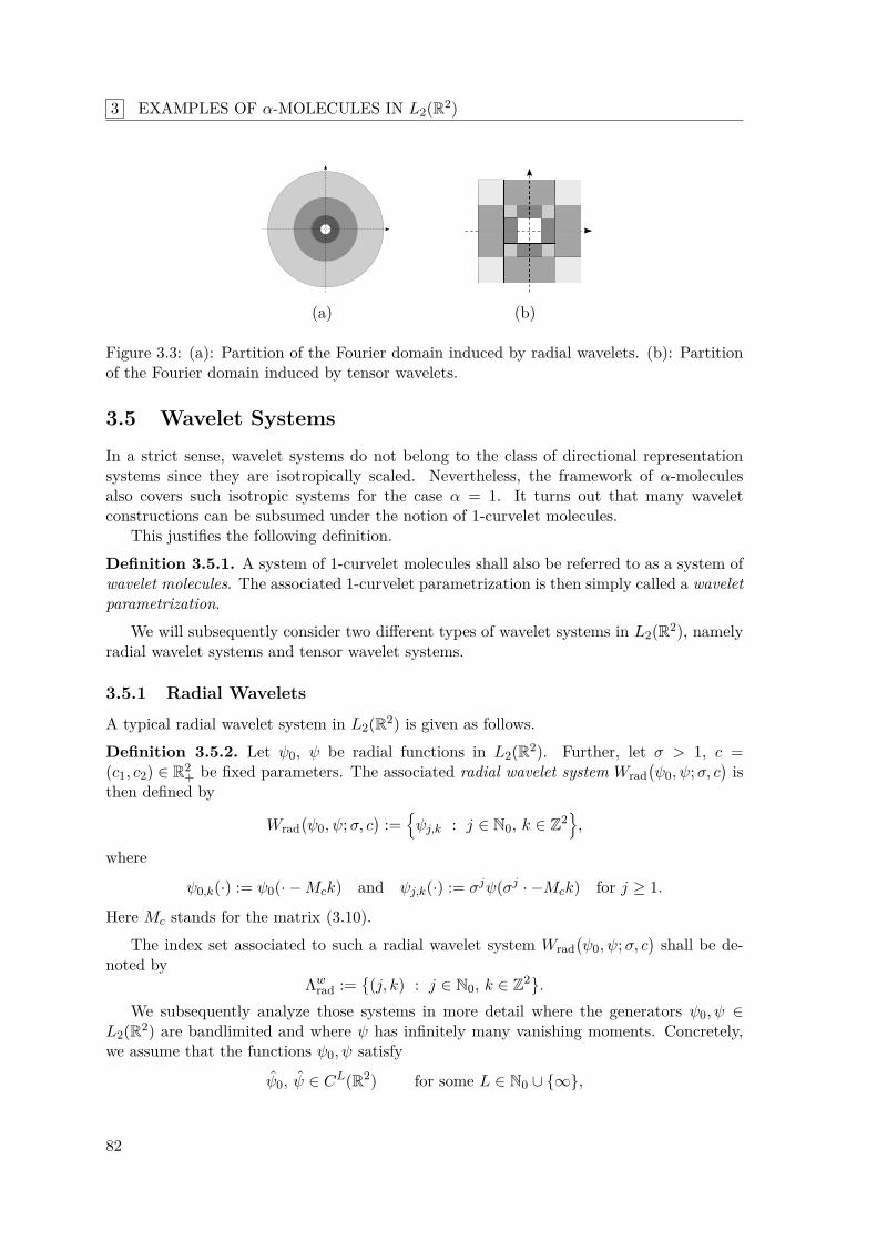
3 EXAMPLES OF α-MOLECULES IN L2(R2)
(a) (b)
Figure 3.3: (a): Partition of the Fourier domain induced by radial wavelets. (b): Partitionof the Fourier domain induced by tensor wavelets.
3.5 Wavelet Systems
In a strict sense, wavelet systems do not belong to the class of directional representationsystems since they are isotropically scaled. Nevertheless, the framework of α-moleculesalso covers such isotropic systems for the case α = 1. It turns out that many waveletconstructions can be subsumed under the notion of 1-curvelet molecules.
This justifies the following definition.
Definition 3.5.1. A system of 1-curvelet molecules shall also be referred to as a system ofwavelet molecules. The associated 1-curvelet parametrization is then simply called a waveletparametrization.
We will subsequently consider two different types of wavelet systems in L2(R2), namelyradial wavelet systems and tensor wavelet systems.
3.5.1 Radial Wavelets
A typical radial wavelet system in L2(R2) is given as follows.
Definition 3.5.2. Let ψ0, ψ be radial functions in L2(R2). Further, let σ > 1, c =(c1, c2) ∈ R2
+ be fixed parameters. The associated radial wavelet system Wradψ0, ψ;σ, c
is
then defined by
Wradψ0, ψ;σ, c
:=ψj,k : j ∈ N0, k ∈ Z2
,
where
ψ0,k(·) := ψ0(· −Mck) and ψj,k(·) := σjψ(σj · −Mck) for j ≥ 1.
Here Mc stands for the matrix (3.10).
The index set associated to such a radial wavelet system Wradψ0, ψ;σ, c
shall be de-
noted byΛw
rad :=(j, k) : j ∈ N0, k ∈ Z2.
We subsequently analyze those systems in more detail where the generators ψ0, ψ ∈L2(R2) are bandlimited and where ψ has infinitely many vanishing moments. Concretely,we assume that the functions ψ0, ψ satisfy
ψ0, ψ ∈ CL(R2) for some L ∈ N0 ∪ ∞,
82
3.5 Wavelet Systems
and that there exist 0 < a and 0 < b < c such that
supp ψ0 ⊆ Ba := ξ ∈ R2 : |ξ| ≤ a and supp ψ ⊆ Cb,c := ξ ∈ R2 : b ≤ |ξ| ≤ c.
According to the following proposition, under these assumptions Wrad(ψ0, ψ;σ, c) is a systemof 1-molecules of order (L,∞,∞,∞). The corresponding tiling of the frequency plane isillustrated in Figure 3.3 (a).
Proposition 3.5.3. Suppose that the generators of the radial wavelet system Wrad(ψ0, ψ;σ, c)fulfill the conditions specified above. Then this system is a system of 1-molecules of order(L,∞,∞,∞) with respect to the radial wavelet parametrization (Λw
rad,Φwrad) with parametriza-
tion mapΦw
rad : Λwrad → P, (j, k) →→ (σ−jMck, 0, σ−j).
Proof. The proof is analogous to the proof of Proposition 3.2.8 (ii).
We next observe that the system Wrad(ψ0, ψ;σ, c) can even be interpreted as a systemof 1-curvelet molecules of order (L,∞,∞,∞), with associated parametrization (Λc,Φc) andparameters σ, c = (c1, c2), as well as Lj := 0 and ωj := 2π for every j ∈ N0 (see (3.11) and(3.13)). For this, we just need to relabel the elements of Wrad(ψ0, ψ;σ, c) via the bijection
ιrad : Λwrad → Λc , (j, k) →→ (j, 0, k).
The relation between the radial wavelet parametrization (Λwrad,Φw
rad) and the corresponding1-curvelet parametrization (Λc,Φc) is then given by
Φwrad = Φc ιrad.
As an immediate consequence, we can derive the following consistency result from The-orem 3.4.3.
Proposition 3.5.4. Let N > 2. Then, with (Λwrad,Φw
rad) being the radial wavelet parametriza-tion, we have
supy∈P
λ∈Λw
rad
ωα(Φwrad(λ),y)−N < ∞.
In particular, the parametrization (Λwrad,Φw
rad) is (1, k)-consistent with other 1-curveletand 1-shearlet parametrizations for k > 2 (compare Corollary 3.4.4).
3.5.2 Tensor Wavelets
Another important class of wavelets in L2(R2) is obtained via tensoring of univariatewavelets. We subsequently recall the tensor product construction from [114]. It buildsupon a given multi-resolution analysis for L2(R) whose scaling function and associatedwavelet shall be denoted by φ0 ∈ L2(R) and φ1 ∈ L2(R), respectively. For every indexe = (e1, e2) ∈ E, where E = 0, 12, one then defines the functions ψe ∈ L2(R2) as thetensor products
ψe = φe1 ⊗ φe2 . (3.50)
These serve as the generators for the tensor wavelet system Wtenφ0, φ1;σ, c
defined below.
83
3 EXAMPLES OF α-MOLECULES IN L2(R2)
Definition 3.5.5. Let φ0, φ1 ∈ L2(R) and ψe ∈ L2(R2), e ∈ E, be defined as above.Further, let σ > 1, c = (c1, c2) ∈ R2
+ be fixed parameters. The associated tensor waveletsystem Wten
φ0, φ1;σ, c
is then defined by
Wtenφ0, φ1;σ, c
:=ψ(0,0)(· −Mck) : k ∈ Z2
∪σjψe(σj · −Mck) : e ∈ E\(0, 0), j ∈ N0, k ∈ Z2
.
Let us now assume that the generating functions φ0, φ1 ∈ L2(R) satisfy
φ0, φ1 ∈ CL(R) for some L ∈ N0 ∪ ∞, (3.51)
and that there exist 0 < a and 0 < b < c such that
supp φ0 ⊂ [−a, a] =: J (0) and supp φ1 ⊂ [−c, c]\[−b, b] =: J (1). (3.52)
Then Wten(φ0, φ1;σ, c) induces a frequency tiling as in Figure 3.3 (b) and, as shown bythe following proposition, this tensor wavelet system is a special instance of a 1-moleculesystem.
Proposition 3.5.6. Let σ > 1, c = (c1, c2) ∈ R2+ be fixed, and assume that the functions
φ0, φ1 satisfy (3.51) and (3.52). Then the tensor wavelet system Wten(φ0, φ1;σ, c) con-stitutes a system of 1-molecules of order (L,∞,∞,∞) with respect to the tensor waveletparametrization (Λw
ten,Φwten) where
Λwten :=
((0, 0), 0, k) : k ∈ Z2 ∪
(e, j, k) : e ∈ E\(0, 0), j ∈ N0, k ∈ Z2
andΦw
ten : Λwten → P, (e, j, k) →→ (σ−jMck, 0, σ−j).
Proof. For (e, j, k) ∈ Λwten we define the generators ge,j,k := ψe, with ψe being the functions
from (3.50). We then have ge,j,k = ψe ∈ CL(R2) by (3.51). Further, (3.52) implies that
supp ψe ⊆ Je := J (e1) × J (e2) for all e = (e1, e2) ∈ E.
Hence supp (∂ρge,j,k) ⊆ Je for every ρ ∈ N20 with |ρ|1 ≤ L and for all (e, j, k) ∈ Λw
ten.Further, the expression supξ∈R2 |∂ρge,j,k(ξ)| = supξ∈R2 |∂ρψe(ξ)| is bounded uniformly in(e, j, k) ∈ Λw
ten. Altogether, this proves that the functions ge,j,k satisfy condition (2.5).Since the wavelets can be written in the form
ψej,k(·) := σjψe(σj · −Mck) = σjge,j,k(σj(· − σ−jMck)),
the proof is finished.
We remark that conditions as in (3.51) and (3.52) are fulfilled, for instance, if φ0, φ1 ∈L2(R) are the generators of a Lemarié-Meyer wavelet system. Moreover, results similar toProposition 3.5.6 can be proven for other wavelet systems of the form Wten(φ0, φ1;σ, c),including systems generated by compactly supported functions φ0 and φ1.
Finally, let us again interpret Wten(φ0, φ1;σ, c) as an instance of a 1-curvelet moleculesystem with parametrization (Λc,Φc). To this end, we choose Lj := 2 and ωj := 2π for all
84
3.6 Ridgelet Systems
j ∈ N0. Further, we use L0 := −1, 0, 1, 2 and Lj := −1, 0, 1 for j ≥ 1 in the definition(3.12) of the 1-curvelet index set Λc. Then
ιten : Λwten → Λc , (e, j, k) →→
(j, e1 − e2, k), e ∈ E\(0, 0),(0, 2, k), e = (0, 0),
is a bijection andΦw
ten = Φc ιten.
Analogous to Proposition 3.5.4, we can derive the canonical consistency of the tensorwavelet parametrization.
Proposition 3.5.7. Let N > 2. Then, with (Λwten,Φw
ten) being the tensor wavelet parametriza-tion, we have
supy∈P
λ∈Λw
ten
ωα(Φwten(λ),y)−N < ∞.
Hence, like the radial wavelet parametrization, the tensor wavelet parametrization is(1, k)-consistent for k > 2 with other 1-curvelet and 1-shearlet parametrizations. Moreover,this result shows that both wavelet parametrizations are (1, k)-consistent, k > 2, with eachother.
3.6 Ridgelet Systems
The last section of this chapter is devoted to ridgelet systems. Whereas there does notexist a common definition of a ridgelet, the different variants of this notion that occur inthe literature are all related to the concept of a so-called ridge function. In the bivariatesetting, this is a function Φ : R2 → C which only varies in one coordinate direction andcan thus be represented in the form Φ = φ(⟨ν, ·⟩) using a suitable univariate profile φ anda direction vector ν ∈ R2.
The term ‘ridgelet’ was first used by Candès in [8] to refer to such bivariate ridgefunctions forming a system of the type
√tφ(⟨teη, ·⟩ − x), eη ∈ S1, x ∈ R2, t ∈ R+, (3.53)
where the profile φ is a univariate wavelet. Systems of this kind can be used for exampleto analyze functions and give rise to the so-called ridgelet transform. A viable theory forthis transform has been developed in [8]. One difficulty, however, when dealing with these‘pure ridgelets’ is their lack of integrability.
In order to obtain system in L2(R2), Donoho slightly relaxed the original definition,allowing the ridgelets a slow decay along the ridge. Using this idea, he constructed anorthonormal basis for L2(R2) whose elements he called ‘orthonormal ridgelets’ [36]. Theirrelationship to the original ‘pure ridgelets’ in the sense of Candès has been analyzed in [37].
An alternative approach to define ridgelet systems in L2(R2) goes back to Grohs [57].He considers function systems of the form
y →→√tψ(A0,tRηy − x), (3.54)
85
3 EXAMPLES OF α-MOLECULES IN L2(R2)
obtained by applying dilations A0,t = diag(t, 1) ∈ R2×2 with t ∈ R+, rotations Rη, η ∈ T,and translations to some generator ψ ∈ L2(R2), which is assumed to be oscillatory in onecoordinate direction. The construction principle is thus the same as for 0-curvelets andclosely resembles (3.53). In fact, the ridgelet construction in [57] more or less coincides withthe 0-curvelet frame C•
0 from Subsection 3.2.3.To ensure the frame property, the scaling is not carried out in Cartesian coordinates,
but in polar coordinates. This causes the ridgelet generators to vary with the scale as wasthe case for C•
0 (see (3.25)). By relaxing the rigid construction principle (3.54) and allowingvariable generators, one then again arrives at the notion of 0-curvelet molecules.
For convenience, we thus make the following definition.
Definition 3.6.1. A system of 0-curvelet molecules is also called a system of ridgeletmolecules. The associated 0-curvelet parametrization is then accordingly referred to as aridgelet parametrization.
Due to Proposition 3.2.4, ridgelet molecules in the above sense are special instances of0-molecules. Further, due to Proposition 3.2.8, the 0-curvelet frame C•
0 from Definition 3.2.6is a special case of a ridgelet molecule system.
Proposition 3.6.2 ([59, Prop. 3.5]). The 0-curvelet frame C•0 is a system of ridgelet
molecules of order (∞,∞,∞,∞).
Summarizing, we can record that ridgelet-type systems in the sense of (3.54) conve-niently fit into the already existing theory. They are covered by the notion of α-curveletmolecules for α = 0.
86
Chapter 4
α-Molecule Coorbit Spaces
In this chapter, we build upon the continuous Parseval frame of α-curvelets Cα = ψxx∈Xfrom Section 3.1 to introduce an associated transform which is a direct generalization of thecontinuous curvelet transform from [10, Sec. 2]. Subsequently it will be called the continuousα-curvelet transform.
Utilizing the coorbit theory put forward in [74], which does not require an underlyinggroup structure of the voice transform, we then define associated α-curvelet coorbit spaces.Further, based on the more general concept of a continuous α-molecule transform, which inparticular comprises the cone-adapted α-shearlet transform, we will also introduce so-calledα-molecule coorbit spaces.
In Theorem 4.3.8 it is shown that those are equivalent to the α-curvelet coorbits. InTheorem 4.3.13 we further give a discrete characterization which identifies them with knownsmoothness spaces, for example from [85]. As an application of the abstract machineryavailable for coorbit spaces, we deduce two further discretization results, Theorem 4.4.19and Theorem 4.4.21, yielding atomic decompositions as well as quasi-Banach frames.
4.1 The Continuous α-Curvelet Transform
In Section 3.1 of Chapter 3 we have constructed the continuous Parseval frame of α-curveletsCα = ψxx∈X, whose index set
X = R2 × T × (0, 1]
can be viewed as a subspace of the parameter domain P defined in (2.1). However, recallthat the topology on X shall not be the subspace topology induced by P. Instead, we willthink of X as being assembled as a disconnected union X = X0 ∪ X1 of two components,namely the homogeneous component X0 and the inhomogeneous component X1 given by
X0 := R2 × T × (0, 1) and X1 := R2 × T × 1.
Each of these components shall thereby carry the subspace topology inherited from P. Asnoted in Section 3.1, X is then a locally compact Hausdorff space.
Further, X is equipped with the Radon measure µ defined by (3.7) satisfying suppµ = X.Its restrictions to the components X0 and X1 are denoted by µ0 and µ1. They are given by
dµ0(x, η, t) = dx dη dt
t3and dµ1(x, η, 1) = dη dt.
We have already shown in Section 3.1 that with respect to this measure Cα is a continuousParseval frame satisfying the Parseval identity (3.5) and the reconstruction formula (3.6).These are important relations, since in the following we want to use the frame Cα as a toolfor signal analysis.
87
4 α-MOLECULE COORBIT SPACES
4.1.1 Basic Transform on L2(R2)In the context of coorbit theory, the analysis operator of a frame is usually called the voicetransform. For the frame Cα = ψxx∈X it takes the form
VCα : L2(R2) → L2(X) , VCαf(x) := ⟨f, ψx⟩, x ∈ X. (4.1)
Subsequently it will be called the continuous α-curvelet transform. Since Cα is a Parsevalframe it defines an isometry from L2(R2) to L2(X).
The corresponding synthesis operator V ∗Cα
is the Hilbert-adjoint of VCα given by
V ∗Cα
: L2(X) → L2(R2) , V ∗CαF =
XF (x)ψx dµ(x).
Hereby the integral is in general only defined in a weak sense.Due to the Parseval property, the associated frame operator, which by definition is the
composition of the analysis and the synthesis operator, is the identity. In other words, forall f ∈ L2(R2) we have the reconstruction formula
f = V ∗CαVCαf =
XVCαf(x)ψx dµ(x), (4.2)
where again the integral is usually only a weak integral in L2(R2).Let us finally take a look at the associated Gramian matrix G[Cα] introduced in (2.7).
It has the entriesG[Cα](x,y) = ⟨ψy, ψx⟩ , x,y ∈ X,
and gives rise to the so-called Gramian operator G[Cα] : L2(X) → L2(X) with
G[Cα]F (x) =X
G[Cα](x,y)F (y) dµ(y) , x ∈ X.
Taking the role of an integral kernel, the Gramian matrix is often referred to as the Gramiankernel. Also note that, for simplicity, we do not distinguish between the Gramian kerneland the Gramian operator in the notation.
From (4.2) we can derive the following reproducing formula, valid for all f ∈ L2(R2),
VCαf(x) =X
G[Cα](x,y)VCαf(y) dµ(y) , x ∈ X. (4.3)
We next turn to an extension of VCα to the space of tempered distributions S ′(R2).
4.1.2 Extension to S ′(R2)As it stands, the α-curvelet transform (4.1) is only defined for square-integrable functionsf ∈ L2(R2). For applications in signal analysis, this is a severe limitation since many signalsof interest are not square-integrable. Therefore, in order to enhance the applicability of VCα ,we need to find a way to extend its definition beyond L2(R2).
A larger reservoir of signals is given by the space of tempered distributions S ′(R2),the topological dual of the Schwartz space S(R2). Its elements, the so-called tempereddistributions, are the continuous linear functionals on S(R2) which is the space of functions
S(R2) :=f ∈ C∞(R2) : |f |κ,ν < ∞ for all (κ, ν) ∈ N2
0 × N20
,
88
4.1 The Continuous α-Curvelet Transform
topologized by the family of semi-norms
|f |κ,ν := supx∈R2
xκ∂νf(x) , κ, ν ∈ N2
0. (4.4)
Equipped with the topology induced by the collection | · |κ,ν : κ, ν ∈ N20, the space S(R2)
becomes a locally convex Hausdorff space.An alternative way to define the topology of S(R2) is to use the collection of norms
∥ · ∥N : N ∈ N0 given by
∥f∥N := supx∈R2
(1 + |x|)N
|γ|≤N
|∂γf(x)|. (4.5)
This collection constitutes a complete filtrating family of norms (see e.g. [72]) generatingthe topology of S(R2). Using these norms, we can easily derive a metric for S(R2) which isconsistent with this topology. It is given by
d(f, g) :=
N∈N0
2−N ∥f − g∥N
1 + ∥f − g∥Nfor f, g ∈ S(R2).
The relation of the spaces S(R2) and S ′(R2) to the Hilbert space L2(R2) is illustratedby the following chain of embeddings
S(R2) ι→ L2(R2) R
→ L2(R2)′ ι∗→ S ′(R2), (4.6)
where ι : S(R2) → L2(R2) is the canonical injection, ι∗ : L2(R2)′ → S ′(R2) its adjoint, andR : L2(R2) → L2(R2)′ denotes the Riesz map between L2(R2) and its dual L2(R2)′, i.e., thecanonical conjugate-linear isomorphism given by f →→ ⟨·, f⟩.
The duality product ⟨·, ·⟩S′×S on the pair S ′(R2)×S(R2) provides a natural way to extendVCα to S ′(R2). Crucial for this is the observation that Cα is contained in S(R2). In fact,the α-curvelets ψx,η,t ∈ Cα are band-limited functions which even satisfy ψx,η,t ∈ C∞
c (R2).This implies ψx,η,t ∈ S(R2) for all (x, η, t) ∈ X and allows to define the extended transformVCα for f ∈ S ′(R2) as
VCαf(x) := ⟨f, ψx⟩S′×S , x ∈ X. (4.7)
This transform VCα “extends” the L2-version from (4.1) in the sense depicted in the followingcommutative diagram:
L2(R2)VCα
−−−−→ L2(X)
R (·)
L2(R2)′VCα
−−−−→ L2(X) .
(4.8)
However, even with this extended definition of VCα at hand, it is not yet clear howuseful this transform actually is for the analysis of signals in S ′(R2). In particular, it isnot a-priori self-evident that VCα is still injective, a prerequisite if we want to be able touniquely reconstruct signals from their transforms.
Fortunately, it turns out that even in its extended form the injectivity of the transformVCα is guaranteed. This is a consequence of the fact that Cα is total in S(R2), i.e., that the
89
4 α-MOLECULE COORBIT SPACES
linear span of Cα is dense in S(R2). This will be the statement of Lemma 4.1.3, but beforewe can give a proof of this we need some preparation.
For every N ∈ N0, let us introduce the auxiliary spaces
BN (R2) :=f ∈ CN (R2) : ∥f∥N < ∞
where ∥ · ∥N is given as in (4.5). These spaces are Banach spaces as the following lemmashows. They are useful since they “approximate” S(R2) in the following sense:
BN+1(R2) ⊂ BN (R2) for N ∈ N0 and S(R2) =
N∈N0
BN (R2).
Moreover, the family of nested spaces BN (R2)N∈N0 captures the topology of S(R2).
Lemma 4.1.1. For each N ∈ N0 the space BN (R2) equipped with the norm ∥ · ∥N is aBanach space. Moreover, if N ≥ 2 it is continuously and densely embedded into L2(R2).
Proof. The vector space properties of BN are obvious. Further, ∥ ·∥N clearly defines a normon BN . To prove the completeness of BN , note that BN → CN . Hence, every Cauchysequence (fn)n∈N ⊂ BN has at least a CN -limit f ∈ CN with ∥fn − f∥CN → 0 for n → ∞.It remains to show f ∈ BN and fn → f in BN .
For this, let ε > 0 be arbitrary. Then there exists M ∈ N such that ∥fn − fm∥N ≤ ε forall n,m ≥ M . From ∥fn − f∥CN → 0 we deduce ∂γfn(x) → ∂γf(x) pointwise for all x ∈ R2
and |γ| ≤ N . By continuity, we deduce for n ≥ M
(1 + |x|)N
|γ|≤N
|∂γ(f − fn)(x)| ≤ ε for all x ∈ R2.
It follows ∥f − fn∥N ≤ ε for all n ≥ M , which implies f ∈ BN since in particular ∥f∥N ≤∥fM ∥N +∥f−fM ∥N < ∞. In addition, we can conclude fn → f in BN since ε was arbitrary.
For f ∈ BN we have f(x) . (1 + |x|)−N . Hence, if N ≥ 2, we clearly have f ∈ L2.Further, BN is dense in L2 due to the density of the subspace C∞
c . Finally, to see that theembedding BN → L2 is continuous, we estimate
∥f |L2∥ ≤ ∥f(1 + | · |)N |L∞∥∥(1 + | · |)−N |L2∥ . ∥f∥N .
Next, we establish a strong form of the reconstruction formula (4.2) for Schwartz func-tions ϕ ∈ S(R2).
Lemma 4.1.2. Let ϕ ∈ S(R2). Then, for every N ∈ N0 the reconstruction formula
ϕ =XVCαϕ(x)ψx dµ(x)
holds in strong Bochner sense in BN (R2).
Proof. Let N ∈ N0. We first prove that the integral converges in Bochner sense in BN . Forthis we verify the Bochner criterion
X|VCαϕ(x)|∥ψx∥N dµ(x) < ∞.
90
4.1 The Continuous α-Curvelet Transform
The integrand of this integral is clearly measurable. It thus only remains to prove theboundedness. To this end, we first show that there is a constant CN > 0 such that
∥ψx∥N ≤ CN t−(1+α)/2t−N (1 + |x|2)N uniformly for all x = (x, η, t) ∈ X. (4.9)
Recall that with gt given as in (3.9)
ψx,η,t = t−(1+α)/2gtA−1
α,tRη(· − x),
which impliesψx,η,t = t(1+α)/2gt
Aα,tRη ·
exp(−2πi⟨x, ·⟩).
Let us now estimate the Schwartz semi-norms |·|κ,ν from (4.4) for the α-curvelets ψx,η,t ∈ Cα.For κ = (κ1, κ2) ∈ N2
0 and ν = (ν1, ν2) ∈ N20, with |κ|1, |ν|1 ≤ N , we have
|ψx,η,t|κ,ν = supξ∈R2
|ξκ∂νψx,η,t(ξ)| .∂κ(ξνψx,η,t)|L1
.Further∂κξ →→ ξνψx,η,t(ξ)|L1
. t(1+α)/2∂κξ →→ ξν gt(Aα,tRηξ) exp(−2πi⟨x, ξ⟩)
|L1
. t(1+α)/2 supl≤κ
∂lξ →→ ξν gt(Aα,tRηξ)|L1|x1|κ1−l1 |x2|κ2−l2
≤ t(1+α)/2(1 + |x|2)N sup|l|1≤N
∂lξ →→ ξν gt(Aα,tRηξ)|L1,
where we used |x1| ≤ |x|2 and |x2| ≤ |x|2 to obtain
|x1|κ1−l1 |x2|κ2−l2 ≤ (1 + |x1|)κ1−l1(1 + |x2|)κ2−l2 ≤ (1 + |x|2)κ1+κ2 ≤ (1 + |x|2)N .
Finally, for l = (l1, l2) ∈ N20 with |l|1 ≤ N we deduce∂lξν gt(Aα,tRη·)
|L1 . sup
m≤minl,ν
ξν−m∂l−mgt(Aα,tRη·)|L1.
Taking into account t ∈ (0, 1], we can estimate∂l−mgt(Aα,tRη·) .
|n|1≤N
∂ngt(Aα,tRη·)
.Using |ξν−m| ≤ (1+ |ξ|2)N , we then obtain for each m = (m1,m2) ∈ N2
0 with m ≤ minl, νξν−m∂l−mgt(Aα,tRη·)|L1 .
|n|1≤N
(1 + |ξ|2)N∂ngt(Aα,tRη·)|L1
= t−(1+α)
|n|1≤N
(1 + |R−1η A−1
α,tξ|2)N∂ngt(·)|L1
. t−(1+α)t−N sup
|n|1≤N
(1 + |ξ|2)N∂ngt(·)|L1
.
91
4 α-MOLECULE COORBIT SPACES
Putting everything together, this yields
|ψx,η,t|κ,ν .∂κ(ξνψx,η,t)|L1
. t−(1+α)/2t−N (1 + |x|2)N sup|n|1≤N
(1 + |ξ|2)N∂ngt(·)|L1
.Now we use the α-molecule estimate (2.5) with N1 > N + 2 and obtain the desired result,
|ψx,η,t|κ,ν . t−(1+α)/2(1 + |x|2)N t−Nξ →→ (1 + |ξ|2)N (1 + |ξ|22)−N1/2|L1
.Finally, we note that uniformly in (x, η, t) ∈ X
∥ψx,η,t∥N . sup|κ|1,|ν|1≤N
|ψx,η,t|κ,ν .
This proves (4.9).Next, we interpret ϕ ∈ S(R2) as a system of α-molecules of order (∞,∞,∞,∞) con-
sisting of just one element with the phase space coordinates (0, 0, 1) ∈ P. Then we obtainfrom Theorem 2.2.2 for arbitrary but fixed N > 0 the estimate
|VCαϕ(x, η, t)| = |⟨ϕ,ψx,η,t⟩| ≤ CN,ϕ · tN (1 + |x|2)−N (4.10)
with a constant CN,ϕ > 0 independent of (x, η, t).Altogether, (4.9) and (4.10) prove the Bochner criterion. Hence the integral
ϕN :=XVCαϕ(x)ψx dµ(x) (4.11)
converges in Bochner sense to a function ϕN in BN . It remains to prove ϕ = ϕN .Let us first assume N ≥ 2. Then BN → L2 and the function ϕN is also the (strong
and weak) L2-limit of this integral. This implies ϕN = ϕ almost everywhere since thereconstruction formula (4.2) holds weakly in L2. Moreover, since both, ϕN ∈ BN andϕ ∈ S, are continuous, we even have pointwise equality. For the case N ∈ 0, 1, let us notethat BN+1 → BN for all N ∈ N0. Altogether, this establishes the reconstruction formula instrong sense in BN for all N ∈ N0.
With the previous result, we are now ready to give a proof of Lemma 4.1.3.
Lemma 4.1.3. The continuous α-curvelet frame Cα is total in S(R2).
Proof. We have seen that the reconstruction formula (4.11) holds in a strong Bochner sensein BN for functions in S. Let U ⊂ S be an open neighborhood in S of some ϕ ∈ S. ThenU is open in BN for sufficiently large N . Since the formula (4.11) holds strongly in BN , wecan deduce that U ∩ spanCα = ∅.
As a consequence of Lemma 4.1.3, the extension of VCα defined in (4.7) is injective onS ′(R2). Hence, it is an invertible transform and the reconstruction of signals is possible. Infact, we have the following reconstruction formula for signals in S ′(R2).
Proposition 4.1.4. For signals f ∈ S ′(R2) the reconstruction formula (4.2) holds ∗-weaklyin S ′(R2), i.e., for all ϕ ∈ S(R2)
⟨f, ϕ⟩S′×S =XVCαf(x)⟨ϕ,ψx⟩ dµ(x). (4.12)
92
4.2 QBF-Spaces on the Curvelet Domain
Proof. We have already observed that ∥ · ∥N N∈N0 is a filtrating family of semi-norms,which generates the topology of S. Hence, according to a fundamental result on continuousfunctionals on locally convex spaces (see e.g. [105, page 96]), for fixed f ∈ S ′(R2) there existcorresponding Nf ∈ N0 and Cf > 0 such that
|⟨f, ϕ⟩S′×S | ≤ Cf ∥ϕ∥Nf= Cf sup
x∈R2(1 + |x|)Nf
|γ|≤Nf
|∂γϕ(x)| for all ϕ ∈ S.
Since S(R2) → BNf(R2), we can thus extend f to a functional f ∈ B′
Nf(R2) by the
Hahn-Banach extension theorem (see e.g. [112, Satz VIII.2.8]). Moreover, if N ≥ 2, wehave the embeddings
S(R2) → BN (R2) → L2(R2) and L2(R2)′ → B′N (R2) → S ′(R2).
Hence, using Lemma 4.1.2, we can argue as follows with N = Nf ,
⟨f, ϕ⟩S′×S = ⟨f , ϕ⟩B′N ×BN
=f ,
XVCαϕ(x)ψx dµ(x)
B′
N ×BN
=XVCαϕ(x)⟨f , ψx⟩B′
N ×BNdµ(x) =
XVCαϕ(x)⟨f, ψx⟩S′×S dµ(x) .
This establishes the reconstruction formula (4.12).
Finally, we also extend the reproducing formula (4.3) to all tempered distributions.
Proposition 4.1.5. The reproducing formula (4.3) holds for tempered distributions, i.e.,for all f ∈ S ′(R2)
VCαf(x) =X
G[Cα](x,y)VCαf(y) dµ(y) , x ∈ X.
Proof. By plugging in ψx for ϕ in (4.12) we directly obtain
VCαf(x) = ⟨f, ψx⟩S′×S =XVCαf(y)⟨ψx, ψy⟩ dµ(y)
=X
G[Cα](x,y)VCαf(y) dµ(y) = G[Cα]VCαf(x),
pointwise for all x ∈ X.
Note that in contrast to (4.3) we need to use the conjugate reproducing kernel G[Cα].This is a consequence of the relation between the extended version of the α-curvelet trans-form (4.7) and the L2-version (4.1), as depicted in (4.8).
4.2 QBF-Spaces on the Curvelet Domain
The continuous α-curvelet transform VCα defined in Section 4.1 is a powerful tool for signalanalysis. In the sequel, we will use its extended version (4.7) for the characterization ofsignals f ∈ S ′(R2) on the transform domain X.
93
4 α-MOLECULE COORBIT SPACES
Concretely, our objects of interest will be so-called α-curvelet coorbit spaces
Co(Cα, Y ) :=f ∈ S ′(R2) : VCαf ∈ Y
, (4.13)
where Y is some suitable function space on X. Our investigation of such spaces will bebased on the theory presented in [74]. One required assumption there is that Y constitutesa rich solid quasi-Banach function space, a notion recalled below.
A quasi-Banach function space, for which we subsequently use the abbreviation QBF-space, with associated domain X is by definition a subset of the µ-measurable functionsfrom X to C, which is linearly closed and complete with respect to some given quasi-norm.Functions which coincide apart from a null-set are thereby identified. In the Banach case,we speak of a Banach function space, or BF-space for short. Note, that QBF-spaces inour sense need not be continuously embedded into Lloc
1 (X) as sometimes required in theliterature, for example in [43].
As a reminder, a quasi-norm on a linear space Y is defined in the same way as a norm,with the only difference that the triangle inequality need not hold in a strict sense. It sufficesif it is satisfied up to a multiplicative constant CY ≥ 1 called the quasi-norm constant, i.e.,if
∥f + g∥ ≤ CY
∥f∥ + ∥g∥
for all f, g ∈ Y.
Another concept, closely related to a quasi-norm, is the notion of an r-norm, where0 < r ≤ 1 and the usual triangle inequality is replaced by the r-triangle inequality
∥f + g∥r ≤ ∥f∥r + ∥g∥r for all f, g ∈ Y.
It is straightforward to show that every r-norm on Y constitutes a quasi-norm with asso-ciated quasi-norm constant CY = 21/r−1. Vice versa, while a quasi-norm need not be anr-norm itself, there at least always exists an equivalent r-norm generating the same topologywith r satisfying CY = 21/r−1. This is the statement of the Aoki-Rolewicz theorem [3, 101].As a consequence, every quasi-normed space Y with quasi-norm constant CY can be re-garded as an r-normed space, with r = (log2(CY ) + 1)−1 being the so-called exponent ofY .
A QBF-space Y on X is called solid if for every µ-measurable function f : X → C wehave
|f | ≤ g for some g ∈ Y ⇒ f ∈ Y and ∥f |Y ∥ ≤ ∥g|Y ∥ .
It is called rich if it contains all characteristic functions XU corresponding to compactsubsets U ⊂ X.
The following lemma draws a connection between the convergence of a sequence of func-tions in a solid quasi-normed function space Y to the pointwise convergence of subsequences.
Lemma 4.2.1 ([74, Lem. 2.2]). Let Y be a solid quasi-normed function space on X, andassume that fn → f in Y for a sequence of functions (fn)n∈N. Then for almost all x ∈ Xthere is a subsequence (fnk
)k∈N, whose choice may depend on the particular x ∈ X, suchthat fnk
(x) → f(x).
Proof. Let us assume that fn → f in Y . Then gn := fn − f → 0 in Y or equivalently∥gn|Y ∥ → 0. Since infm≥n |gm| is a measurable function with infm≥n |gm| ≤ |gk| for all
94
4.2 QBF-Spaces on the Curvelet Domain
k ≥ n the solidity of Y yields infm≥n |gm| ∈ Y and ∥ infm≥n |gm||Y ∥ ≤ ∥gk|Y ∥ for all k ≥ n.We deduce
0 ≤ ∥ infm≥n
|gm||Y ∥ ≤ infm≥n
∥gm|Y ∥ = 0,
and as a consequence infm≥n |gm|(x) = 0 for almost every x ∈ X. For each of these x, wecan hence find a subsequence (gnk
)k∈N such that gnk(x) → 0. This implies fnk
(x) → f(x)and yields the result.
We will subsequently restrict our attention to a special scale of function spaces on Xcorresponding to Besov-type characterizations of the signals f ∈ S ′(R2). These spaces canbe viewed as straight-forward generalizations of the mixed-norm Lebesgue spaces used in[111] for the coorbit description of the classic inhomogeneous Besov spaces.
We remark, that also other scales of function spaces on X could be considered, for exam-ple spaces leading to Triebel-Lizorkin type characterizations. The bulk of the subsequentexposition remains the same, significant adaptions are only needed in Subsection 4.5.5.
4.2.1 The Mixed-norm Lebesgue Spaces Lsp,q(X)
We now define a scale Lsp,q(X) of function spaces on X which is inspired by the mixed-norm
Lebesgue spaces on the inhomogeneous wavelet domain R2 × [(0, 1) ∪ ∞], consideredin [111].
Definition 4.2.2. Let 0 < p, q < ∞ and s ∈ R. We then define the function space
Lsp,q(X) :=
F : X → C µ-measurable : ∥F |Ls
p,q∥ < ∞
with respective quasi-norm
∥F |Lsp,q∥ :=
2π
0
F (·, η, 1)Lp
qdη1/q
+ 1
0
2π
0t−sq
F (·, η, t)Lp
q dη dt
t
1/q.
As we will see in Proposition 4.2.4, this space constitutes a rich solid QBF-space on Xwith associated exponent r := min1, p, q. For the proof of the completeness, we will usethe fact that Fatou’s lemma is valid in Ls
p,q(X).
Lemma 4.2.3. Let (Fn)n∈N be a sequence of functions Fn : X → [0,∞) in Lsp,q(X) such
that lim infn→∞ ∥Fn|Lsp,q∥ < ∞. Then F := lim infn→∞ Fn ∈ Ls
p,q(X) with ∥F |Lsp,q∥ ≤
lim infn→∞ ∥Fn|Lsp,q∥.
Proof. The assertion is a direct consequence of the classic lemma of Fatou for Lebesguespaces [2, Lem. A1.20]. For the inhomogeneous part, we obtain
2π
0
lim infn→∞
Fn(·, η, 1)Lp
qdη1/q
≤ 2π
0lim infn→∞
Fn(·, η, 1)Lp
qdη1/q
≤ lim infn→∞
2π
0
Fn(·, η, 1)Lp
qdη1/q
.
The calculation for the homogeneous part is similar.
Now we are ready to prove the following result.
95
4 α-MOLECULE COORBIT SPACES
Proposition 4.2.4. The spaces Lsp,q(X) are rich solid QBF-spaces on X with associated
exponent r := min1, p, q.
Proof. It is straightforward to verify that Lsp,q is a quasi-normed space on X. A direct
calculation with p := p/r, q := q/r, s := sr, namely
∥f + g|Lsp,q∥r = ∥|f + g|r|Ls
p,q∥ ≤ ∥|f |r|Lsp,q∥ + ∥|g|r|Ls
p,q∥ = ∥f |Lsp,q∥r + ∥g|Ls
p,q∥r,
further shows for r := min1, p, q and arbitrary f, g ∈ Lsp,q
∥f + g|Lsp,q∥r ≤ ∥f |Ls
p,q∥r + ∥g|Lsp,q∥r.
As a consequence, ∥ · |Lsp,q∥ is also an r-norm. The solidity of Ls
p,q is obvious. For the proofof the richness, we refer to Lemma 4.2.11.
At last, we prove the completeness of Lsp,q and consider a Cauchy sequence (Fn)n∈N.
Without loss of generality, we may assume the property
∥Fn+1 − Fn|Lsp,q∥ ≤ 2−n/r for all n ∈ N.
We then define the µ-measurable functions
Gm :=m
n=1|Fn+1 − Fn| , m ∈ N,
which are elements of Lsp,q due to the estimate
∥Gm|Lsp,q∥r ≤
mn=1
∥Fn+1 − Fn|Lsp,q∥r ≤
∞n=1
∥Fn+1 − Fn|Lsp,q∥r ≤
∞n=1
2−n = 1.
Further, since the sequence (Gm)m∈N is monotonically increasing, we obtain with Lemma 4.2.3
G := limm→∞
Gm = lim infm→∞
Gm ∈ Lsp,q,
and further∥G|Ls
p,q∥ ≤ lim infm→∞
∥Gm|Lsp,q∥ ≤ 1.
In particular, the function G is finite almost everywhere and the sum∞
n=1 |Fn+1(x) −Fn(x)| converges for almost every x ∈ X. At those points, the sequence (Fn(x))n∈N is aCauchy sequence in C and the limit
F (x) := limn→∞
Fn(x)
is well-defined, giving rise to a µ-measurable function F on X.Using Lemma 4.2.3 and the fact that (Fn)n∈N is a Cauchy sequence in Ls
p,q, we deduce
∥F − Fn|Lsp,q∥ = ∥ lim
m→∞|Fm − Fn||Ls
p,q∥ ≤ lim infm→∞
∥Fm − Fn|Lsp,q∥ → 0 (n → ∞).
This implies F ∈ Lsp,q and the convergence Fn → F in Ls
p,q.
In the next subsection, we introduce another scale of function spaces on X closely relatedto Ls
p,q(X). Those spaces, denoted by Lα,sp,q (X), feature more regularity. For instance, in
contrast to Lsp,q(X), they are continuously embedded into Lloc
1 (X), even in the quasi-Banachcase.
96
4.2 QBF-Spaces on the Curvelet Domain
4.2.2 The Associated Wiener Spaces Lα,sp,q (X)
The Wiener spaces Lα,sp,q (X) are obtained by a Wiener-type amalgamization (see [43, Def. 3.1])
of Lsp,q(X) with the local component L∞(X). This means that we utilize a suitable family of
window functions Wxx∈X to take the L∞-norm locally around points x ∈ X. Afterwards,for a measurable function F : X → C the so-called control function
x →→ ∥XWxF |L∞∥, (4.14)
is measured globally in the Lsp,q-quasi-norm. The outcome of this procedure clearly depends
on the utilized windows and we need to carefully choose those.On the wavelet domain, which naturally carries a group structure, a canonical way to
generate suitable windows is by the action of the group on some fixed prototype window.Since we do not have a group structure on X, we need to take a different route and resortto the quasi-metric structure of X instead. Hence, we use the α-balls Bα
τ (x), or – to thesame effect – their more practical relatives V α
τ (x), defined in (2.25) and (2.26), to localizethe functions around points x ∈ X.
By appropriately restricting the sets in the collection Vατ [X] := V α
τ (x) : x ∈ X, weobtain for each α ∈ [0, 1] and τ ≥ 0 the family
Uατ [X] :=
Uα
τ (x) : x ∈ X
with Uατ (x) :=
V α
τ (x) ∩ X0 , x ∈ X0,
V ατ (x) ∩ X1 , x ∈ X1.
For convenience, let us state the explicit form of these sets,
Uατ (x) =
x+R−1
η Aα,tQτ
×η + t1−αIτ
2π
×tJτ ∩ (0, 1)
, x ∈ X0 ,
x+R−1η Qτ
×η + Iτ
2π
×1
, x ∈ X1 .
where Qτ := [−τ, τ ]2, Iτ := [−τ, τ ], and Jτ := [2−τ , 2τ ]. Utilizing
Qα,τx,η,t := x+R−1
η Aα,tQτ , Iα,τ
η,t :=η + t1−αIτ
2π, Jτ
t :=tJτ ∩ (0, 1) , 0 < t < 1,1 , t = 1,
we can also write
Uατ (x) = Qα,τ
x,η,t × Iα,τη,t × Jτ
t . (4.15)
The corresponding dual sets U ′,ατ (x) are given by
U ′,ατ (x) :=
y ∈ X : x ∈ Uα
τ (y)
=V ′,α
τ (x) ∩ X0 , x ∈ X0,
V ′,ατ (x) ∩ X1 , x ∈ X1,
with
U ′,ατ (x) =
y ∈ X0 : y ∈ x+R−1
θ Aα,uQτ , θ ∈
η + u1−αIτ
2π, u ∈ tJτ
, x ∈ X0 ,
y ∈ X1 : y ∈ x+R−1θ Qτ , θ ∈
η + Iτ
2π
, x ∈ X1 ,
or alternatively
U ′,ατ (x) =
y ∈ X : y ∈ Qα,τ
x,θ,u, θ ∈ Iα,τη,u , u ∈ Jτ
t
. (4.16)
Some elementary but essential properties of the sets Uατ (x) carry over from Lemma 2.2.17.
It is worth noting that the results are now uniform for all x ∈ X. Moreover, they are inde-pendent of α ∈ [0, 1].
97
4 α-MOLECULE COORBIT SPACES
Lemma 4.2.5. Let α ∈ [0, 1] and x = (x, η, t) ∈ X be fixed. For τ ≥ 0 define the functionm(τ) := 2τ (1 + τ). For τ, σ ≥ 0 the following holds true:
i) If τ < σ then Uατ (x) ⊂ Uα
σ (x), and Uα0 (x) =
τ>0 U
ατ (x) = x.
ii) y ∈ Uατ (x) ⇒ x ∈ Uα
τm(τ)(y).
iii) y ∈ Uατ (x) and z ∈ Uα
σ (y) ⇒ z ∈ Uαf(τ,σ)(x) with f(τ, σ) := τ + σm(τ).
iv) y ∈ Uατ (x) and z ∈ Uα
σ (x) ⇒ z ∈ Uαg(τ,σ)(y) with g(τ, σ) := (τ + σ)m(τ).
v) x ∈ Uατ (y) ∩ Uα
σ (z) ⇒ z ∈ Uαh(τ,σ)(y) with h(τ, σ) = τ + σm(τ)m(σ).
Proof. We distinguish two cases, either x ∈ X0 or x ∈ X1. If x ∈ X0 then Uατ (x) = V α
τ (x) ∩X0 and consequently y, z ∈ X0. Analogously, x ∈ X1 implies Uα
τ (x) = V ατ (x) ∩X1 and thus
y, z ∈ X1. Since mt(τ) = m(τ) for t ≤ 1, the assertions follow then from Lemma 2.2.17.
Now we are ready to define the α-anisotropic Wiener maximal operator Wατ depending
on α ∈ [0, 1] and τ > 0. For a function F : X → C we put
Wατ F (x) := ∥FXUα
τ (x)|L∞∥ = ess supy∈Uα
τ (x)|F (y)| , x ∈ X. (4.17)
Further, if τ = 1 we use the simplified notation Wα := Wα1 .
The term maximal operator is justified, since Wατ has the following majorizing property,
|F (x)| ≤ Wατ F (x) for a.e. x ∈ X. (4.18)
But an even stronger result holds true, stated in the following lemma.
Lemma 4.2.6. Let α ∈ [0, 1] and let τ > σ > 0. Then for any function F : X → C we havefor almost every x ∈ X
|F (x)|XUασ (y)(x) = |F (x)|XU ′,α
σ (x)(y) ≤ Wατ F (y) for all y ∈ X.
Proof. In a first step we prove (4.18). For this choose ρ := min1, τ/8 > 0 such thatg(ρ, ρ) ≤ τ , where g is the function from Lemma 4.2.5(iv). According to Lemma 4.2.5(iv),we then have
y∈Uαρ (x)
Uατ (y) ⊇ Uα
ρ (x) for all x ∈ X.
It follows that for each x ∈ X the following relation holds true, for almost all y ∈ Uαρ (x),
|F (y)| ≤ ess supz∈Uα
ρ (x)|F (z)| ≤ ess sup
z∈Uατ (y)
|F (z)| = Wατ F (y).
The relation (4.18) is a direct consequence, since we can find a sequence (xn)n∈N such thatUα
ρ (xn)n∈N is a countable covering of X.Secondly, we now turn to the proof of the more general assertion of the lemma. According
to (4.18), for each n ∈ N there exists a null-set Nn ⊂ X such that |F (x)| ≤ Wα1/nF (x) for
all x ∈ X\Nn. Putting N :=
n Nn, which is again a null-set, we then have |F (x)| ≤Wα
τ F (x) for all x ∈ X\N and all τ > 0. Since by assumption σ < τ , we can choose
98
4.2 QBF-Spaces on the Curvelet Domain
ρ := (τ − σ)/m(σ) > 0 such that f(σ, ρ) = τ for the function f from Lemma 4.2.5(iii).Then for every x ∈ X\N
|F (x)| ≤ WαρF (x) ≤ Wα
τ F (y) for all y ∈ U ′,ασ (x),
where U ′,ασ (x) denotes the dual ball of Uα
σ (x). Since XUασ (y)(x) = XU ′,α
σ (x)(y), the proof isfinished.
Utilizing the maximal operator Wα = Wα1 , we can now define the spaces Lα,s
p,q (X). Notethat in contrast to the original scale Ls
p,q(X) the new scale Lα,sp,q (X) also depends on the
parameter α ∈ [0, 1].
Definition 4.2.7. Let α ∈ [0, 1], 0 < p, q < ∞, and s ∈ R. We define the α-anisotropicWiener space associated to Ls
p,q(X) as
Lα,sp,q (X) :=
F : X → C µ-measurable : ∥WαF |Ls
p,q∥ < ∞
with quasi-norm ∥ · |Lα,sp,q ∥ := ∥Wα(·)|Ls
p,q∥.
The spaces Lα,sp,q (X) inherit many properties from the scale Ls
p,q(X). In particular, likethose, they are rich solid QBF-spaces on X with the same exponent r = min1, p, q. Forthe proof of this fact we need the following commutation property of Wα
τ .
Lemma 4.2.8. Let α ∈ [0, 1] and τ > 0. Assume that Fn → F converges pointwise almosteverywhere for n → ∞, in a uniform way on compacta. Then
Wατ F (x) = lim
n→∞Wα
τ Fn(x) for every x ∈ X.
Proof. First, we show that for any two functions F,G : X → C and all x ∈ X
|WατG(x) − Wα
τ F (x)| ≤ Wατ (G− F )(x). (4.19)
Without loss of generality, we can assume that WατG(x) ≥ Wα
τ F (x). Further, there existsa null-set N ⊂ X such that |F (y)| ≤ ess supz∈Uα
τ (x) |F (z)| for all y ∈ Uατ (x)\N. Then (4.19)
follows from the estimate
ess supy∈Uα
τ (x)|G(y)| − ess sup
z∈Uατ (x)
|F (z)| = ess supy∈Uα
τ (x)\N
|G(y)| − ess sup
z∈Uατ (x)
|F (z)|
≤ ess supy∈Uα
τ (x)\N
|G(y)| − |F (y)|
≤ ess sup
y∈Uατ (x)
|G(y) − F (y)|.
The assertion of the lemma is now a direct consequence of the validity of
|Wατ Fn(x) − Wα
τ F (x)| ≤ Wατ (Fn − F )(x) = ess sup
y∈Uατ (x)
|Fn(y) − F (y)|
for every x ∈ X and the fact that
ess supy∈Uα
τ (x)|Fn(y) − F (y)| → 0 (n → ∞).
Now we formulate the companion result to Proposition 4.2.4.
99
4 α-MOLECULE COORBIT SPACES
Proposition 4.2.9. The spaces Lα,sp,q (X) are rich solid QBF-spaces on X with associated
exponent r := min1, p, q.
Proof. It is clear that Lα,sp,q is a quasi-normed space on X with the same exponent r =
min1, p, q as Lsp,q. Further, the solidity of Lα,s
p,q directly follows from the solidity of Lsp,q
and the monotonicity of the Wiener maximal operator. To verify the richness, we useLemma 4.2.5(v) to estimate
WαXUασ (x) ≤ XUα
h(σ,1)(x) for every x ∈ X and all σ > 0. (4.20)
Taking into account the richness and the solidity of Lsp,q, this implies WαXUα
σ (x) ∈ Lsp,q and
thus XUασ (x) ∈ Lα,s
p,q .It remains to show the completeness of Lα,s
p,q . For this, we use an embedding which willbe established in the next subsection. According to (4.26), we have Lα,s
p,q → Lloc∞ . Due to
this result, every Cauchy sequence (Fn)n∈N in Lα,sp,q yields Cauchy sequences (Fn(x))n∈N in
C for almost every x ∈ X.Hence, (Fn)n∈N converges pointwise almost everywhere to a µ-measurable function F on
X. In addition, the convergence is uniform on compacta. Hence, we can apply Lemma 4.2.8which yields for fixed m ∈ N the pointwise convergence
Wατ
Fm − F
= lim
n→∞Wα
τ (Fm − Fn).
Since (Fn)n∈N is a Cauchy sequence in Lα,sp,q , we can further verify for every m ∈ N
lim infn→∞
∥Wατ (Fm − Fn)|Ls
p,q∥ = lim infn→∞
∥Fm − Fn|Lα,sp,q ∥ < ∞.
Hence, using the Fatou property of Lsp,q proved in Lemma 4.2.3, we get Wα
τ (Fm −F ) ∈ Lsp,q
and thus Fm −F ∈ Lα,sp,q for all m ∈ N. In particular, since Fm ∈ Lα,s
p,q , this implies F ∈ Lα,sp,q .
Further, we have Fm → F in Lα,sp,q since
∥Fm − F |Lα,sp,q ∥ ≤ lim inf
n→∞∥Wα
τ (Fm − Fn)|Lsp,q∥ = lim inf
n→∞∥Fm − Fn|Lα,s
p,q ∥ → 0 (m → ∞).
We end this subsection with an important embedding, relating the spaces Lα,sp,q (X) and
Lsp,q(X). It is a direct consequence of (4.18).
Proposition 4.2.10. We have the continuous embedding
Lα,sp,q (X) → Ls
p,q(X).
Proof. As a consequence of (4.18) and the solidity of Lsp,q, we obtain
∥F |Lsp,q∥ ≤ ∥WαF |Ls
p,q∥ = ∥F |Lα,sp,q ∥
for every measurable function F : X → C. This yields the result.
Another important embedding of Lα,sp,q (X) is derived in the next subsection. Proposi-
tion 4.2.13 will show that these Wiener spaces are naturally embedded into certain weightedL∞-spaces.
100
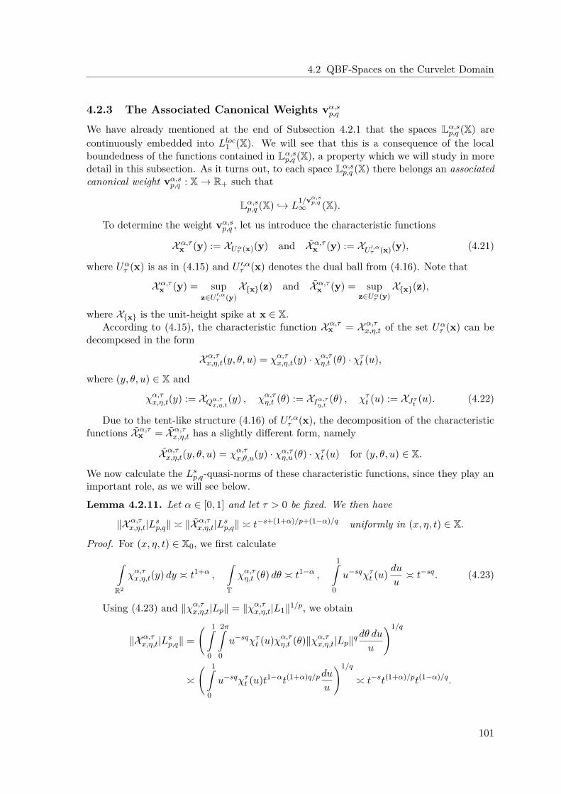
4.2 QBF-Spaces on the Curvelet Domain
4.2.3 The Associated Canonical Weights vα,sp,q
We have already mentioned at the end of Subsection 4.2.1 that the spaces Lα,sp,q (X) are
continuously embedded into Lloc1 (X). We will see that this is a consequence of the local
boundedness of the functions contained in Lα,sp,q (X), a property which we will study in more
detail in this subsection. As it turns out, to each space Lα,sp,q (X) there belongs an associated
canonical weight vα,sp,q : X → R+ such that
Lα,sp,q (X) → L
1/vα,sp,q
∞ (X).
To determine the weight vα,sp,q , let us introduce the characteristic functions
X α,τx (y) := XUα
τ (x)(y) and X α,τx (y) := XU ′,α
τ (x)(y), (4.21)
where Uατ (x) is as in (4.15) and U ′,α
τ (x) denotes the dual ball from (4.16). Note that
X α,τx (y) = sup
z∈U ′,ατ (y)
Xx(z) and X α,τx (y) = sup
z∈Uατ (y)
Xx(z),
where Xx is the unit-height spike at x ∈ X.According to (4.15), the characteristic function X α,τ
x = X α,τx,η,t of the set Uα
τ (x) can bedecomposed in the form
X α,τx,η,t(y, θ, u) = χα,τ
x,η,t(y) · χα,τη,t (θ) · χτ
t (u),
where (y, θ, u) ∈ X and
χα,τx,η,t(y) := XQα,τ
x,η,t(y) , χα,τ
η,t (θ) := XIα,τη,t
(θ) , χτt (u) := XJτ
t(u). (4.22)
Due to the tent-like structure (4.16) of U ′,ατ (x), the decomposition of the characteristic
functions X α,τx = X α,τ
x,η,t has a slightly different form, namely
X α,τx,η,t(y, θ, u) = χα,τ
x,θ,u(y) · χα,τη,u(θ) · χτ
t (u) for (y, θ, u) ∈ X.
We now calculate the Lsp,q-quasi-norms of these characteristic functions, since they play an
important role, as we will see below.
Lemma 4.2.11. Let α ∈ [0, 1] and let τ > 0 be fixed. We then have
∥X α,τx,η,t|Ls
p,q∥ ≍ ∥X α,τx,η,t|Ls
p,q∥ ≍ t−s+(1+α)/p+(1−α)/q uniformly in (x, η, t) ∈ X.
Proof. For (x, η, t) ∈ X0, we first calculate
R2
χα,τx,η,t(y) dy ≍ t1+α ,
T
χα,τη,t (θ) dθ ≍ t1−α ,
10
u−sqχτt (u) du
u≍ t−sq. (4.23)
Using (4.23) and ∥χα,τx,η,t|Lp∥ = ∥χα,τ
x,η,t|L1∥1/p, we obtain
∥X α,τx,η,t|Ls
p,q∥ = 1
0
2π0
u−sqχτt (u)χα,τ
η,t (θ)∥χα,τx,η,t|Lp∥q dθ du
u
1/q
≍ 1
0
u−sqχτt (u)t1−αt(1+α)q/p du
u
1/q
≍ t−st(1+α)/pt(1−α)/q.
101
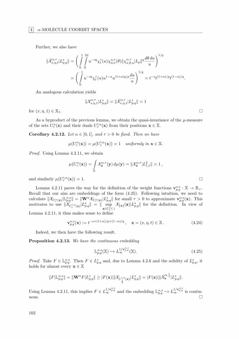
4 α-MOLECULE COORBIT SPACES
Further, we also have
∥X α,τx,η,t|Ls
p,q∥ = 1
0
2π0
u−sqχτt (u)χα,τ
η,u(θ)∥χα,τx,θ,u|Lp∥q dθ du
u
1/q
≍ 1
0
u−sqχτt (u)u1−αu(1+α)q/p du
u
1/q
≍ t−st(1+α)/pt(1−α)/q.
An analogous calculation yields
∥X α,τx,η,1|Ls
p,q∥ ≍ ∥X α,τx,η,1|Ls
p,q∥ ≍ 1
for (x, η, 1) ∈ X1.
As a byproduct of the previous lemma, we obtain the quasi-invariance of the µ-measureof the sets Uα
τ (x) and their duals U ′,ατ (x) from their positions x ∈ X.
Corollary 4.2.12. Let α ∈ [0, 1], and τ > 0 be fixed. Then we have
µUα
τ (x)
≍ µU ′,α
τ (x)
≍ 1 uniformly in x ∈ X.
Proof. Using Lemma 4.2.11, we obtain
µUα
τ (x)
=X
X α,τx (y) dµ(y) = ∥X α,τ
x |L21,1∥ ≍ 1 ,
and similarly µU ′,α
τ (x)
≍ 1.
Lemma 4.2.11 paves the way for the definition of the weight functions vα,sp,q : X → R+.
Recall that our aim are embeddings of the form (4.25). Following intuition, we need tocalculate ∥XUα
τ (x)|Lα,sp,q ∥ = ∥WαXUα
τ (x)|Lsp,q∥ for small τ > 0 to approximate vα,s
p,q (x). Thismotivates to use ∥XU ′,α
1 (x)|Lsp,q∥ = ∥ sup
z∈Uα1 (·)
Xx(z)|Lsp,q∥ for the definition. In view of
Lemma 4.2.11, it thus makes sense to define
vα,sp,q (x) := t−s+(1+α)/p+(1−α)/q , x = (x, η, t) ∈ X . (4.24)
Indeed, we then have the following result.
Proposition 4.2.13. We have the continuous embedding
Lα,sp,q (X) → L
1/vα,sp,q
∞ (X). (4.25)
Proof. Take F ∈ Lα,sp,q . Then F ∈ Ls
p,q and, due to Lemma 4.2.6 and the solidity of Lsp,q, it
holds for almost every x ∈ X
∥F |Lα,sp,q ∥ = ∥WαF |Ls
p,q∥ ≥ |F (x)|∥XU ′,α12
(x)|Lsp,q∥ = |F (x)|∥X α, 1
2x |Lsp,q∥.
Using Lemma 4.2.11, this implies F ∈ L1/vα,s
p,q∞ and the embedding Lα,s
p,q → L1/vα,s
p,q∞ is contin-
uous.
102
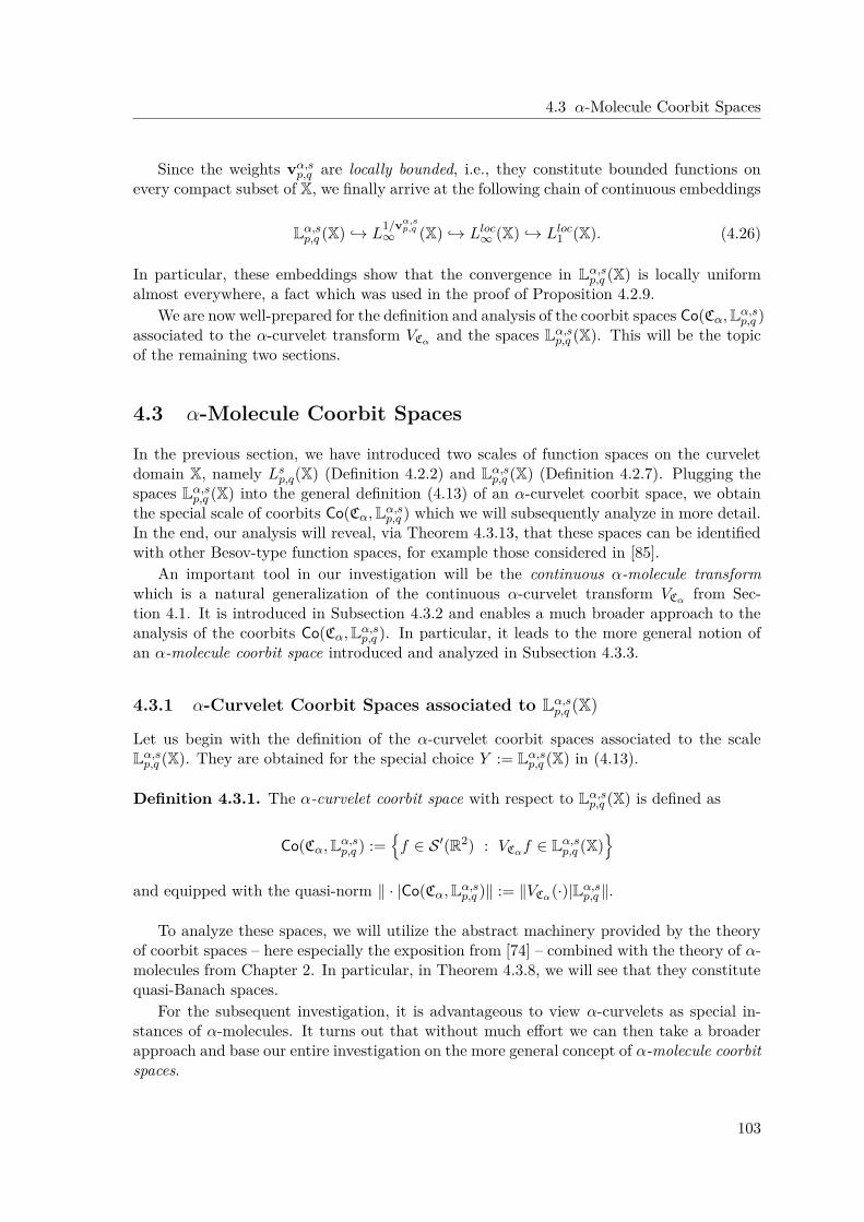
4.3 α-Molecule Coorbit Spaces
Since the weights vα,sp,q are locally bounded, i.e., they constitute bounded functions on
every compact subset of X, we finally arrive at the following chain of continuous embeddings
Lα,sp,q (X) → L
1/vα,sp,q
∞ (X) → Lloc∞ (X) → Lloc
1 (X). (4.26)
In particular, these embeddings show that the convergence in Lα,sp,q (X) is locally uniform
almost everywhere, a fact which was used in the proof of Proposition 4.2.9.We are now well-prepared for the definition and analysis of the coorbit spaces Co(Cα,Lα,s
p,q )associated to the α-curvelet transform VCα and the spaces Lα,s
p,q (X). This will be the topicof the remaining two sections.
4.3 α-Molecule Coorbit Spaces
In the previous section, we have introduced two scales of function spaces on the curveletdomain X, namely Ls
p,q(X) (Definition 4.2.2) and Lα,sp,q (X) (Definition 4.2.7). Plugging the
spaces Lα,sp,q (X) into the general definition (4.13) of an α-curvelet coorbit space, we obtain
the special scale of coorbits Co(Cα,Lα,sp,q ) which we will subsequently analyze in more detail.
In the end, our analysis will reveal, via Theorem 4.3.13, that these spaces can be identifiedwith other Besov-type function spaces, for example those considered in [85].
An important tool in our investigation will be the continuous α-molecule transformwhich is a natural generalization of the continuous α-curvelet transform VCα from Sec-tion 4.1. It is introduced in Subsection 4.3.2 and enables a much broader approach to theanalysis of the coorbits Co(Cα,Lα,s
p,q ). In particular, it leads to the more general notion ofan α-molecule coorbit space introduced and analyzed in Subsection 4.3.3.
4.3.1 α-Curvelet Coorbit Spaces associated to Lα,sp,q (X)
Let us begin with the definition of the α-curvelet coorbit spaces associated to the scaleLα,s
p,q (X). They are obtained for the special choice Y := Lα,sp,q (X) in (4.13).
Definition 4.3.1. The α-curvelet coorbit space with respect to Lα,sp,q (X) is defined as
Co(Cα,Lα,sp,q ) :=
f ∈ S ′(R2) : VCαf ∈ Lα,s
p,q (X)
and equipped with the quasi-norm ∥ · |Co(Cα,Lα,sp,q )∥ := ∥VCα(·)|Lα,s
p,q ∥.
To analyze these spaces, we will utilize the abstract machinery provided by the theoryof coorbit spaces – here especially the exposition from [74] – combined with the theory of α-molecules from Chapter 2. In particular, in Theorem 4.3.8, we will see that they constitutequasi-Banach spaces.
For the subsequent investigation, it is advantageous to view α-curvelets as special in-stances of α-molecules. It turns out that without much effort we can then take a broaderapproach and base our entire investigation on the more general concept of α-molecule coorbitspaces.
103
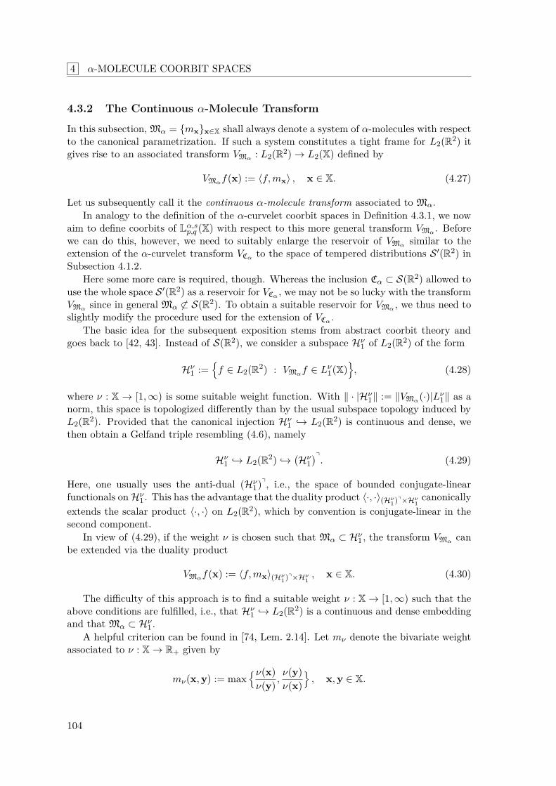
4 α-MOLECULE COORBIT SPACES
4.3.2 The Continuous α-Molecule Transform
In this subsection, Mα = mxx∈X shall always denote a system of α-molecules with respectto the canonical parametrization. If such a system constitutes a tight frame for L2(R2) itgives rise to an associated transform VMα : L2(R2) → L2(X) defined by
VMαf(x) := ⟨f,mx⟩ , x ∈ X. (4.27)
Let us subsequently call it the continuous α-molecule transform associated to Mα.In analogy to the definition of the α-curvelet coorbit spaces in Definition 4.3.1, we now
aim to define coorbits of Lα,sp,q (X) with respect to this more general transform VMα . Before
we can do this, however, we need to suitably enlarge the reservoir of VMα similar to theextension of the α-curvelet transform VCα to the space of tempered distributions S ′(R2) inSubsection 4.1.2.
Here some more care is required, though. Whereas the inclusion Cα ⊂ S(R2) allowed touse the whole space S ′(R2) as a reservoir for VCα , we may not be so lucky with the transformVMα since in general Mα ⊂ S(R2). To obtain a suitable reservoir for VMα , we thus need toslightly modify the procedure used for the extension of VCα .
The basic idea for the subsequent exposition stems from abstract coorbit theory andgoes back to [42, 43]. Instead of S(R2), we consider a subspace Hν
1 of L2(R2) of the form
Hν1 :=
f ∈ L2(R2) : VMαf ∈ Lν
1(X), (4.28)
where ν : X → [1,∞) is some suitable weight function. With ∥ · |Hν1∥ := ∥VMα(·)|Lν
1∥ as anorm, this space is topologized differently than by the usual subspace topology induced byL2(R2). Provided that the canonical injection Hν
1 → L2(R2) is continuous and dense, wethen obtain a Gelfand triple resembling (4.6), namely
Hν1 → L2(R2) →
Hν
1q. (4.29)
Here, one usually uses the anti-dual (Hν1)q, i.e., the space of bounded conjugate-linear
functionals on Hν1 . This has the advantage that the duality product ⟨·, ·⟩(Hν
1 )q×Hν1
canonicallyextends the scalar product ⟨·, ·⟩ on L2(R2), which by convention is conjugate-linear in thesecond component.
In view of (4.29), if the weight ν is chosen such that Mα ⊂ Hν1 , the transform VMα can
be extended via the duality product
VMαf(x) := ⟨f,mx⟩(Hν1 )q×Hν
1, x ∈ X. (4.30)
The difficulty of this approach is to find a suitable weight ν : X → [1,∞) such that theabove conditions are fulfilled, i.e., that Hν
1 → L2(R2) is a continuous and dense embeddingand that Mα ⊂ Hν
1 .A helpful criterion can be found in [74, Lem. 2.14]. Let mν denote the bivariate weight
associated to ν : X → R+ given by
mν(x,y) := maxν(x)ν(y) ,
ν(y)ν(x)
, x,y ∈ X.
104
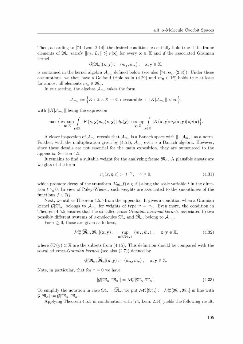
4.3 α-Molecule Coorbit Spaces
Then, according to [74, Lem. 2.14], the desired conditions essentially hold true if the frameelements of Mα satisfy ∥mx|L2∥ . ν(x) for every x ∈ X and if the associated Gramiankernel
G[Mα](x,y) := ⟨my,mx⟩ , x,y ∈ X,
is contained in the kernel algebra Amν defined below (see also [74, eq. (2.8)]). Under theseassumptions, we then have a Gelfand triple as in (4.29) and mx ∈ Hν
1 holds true at leastfor almost all elements mx ∈ Mα.
In our setting, the algebra Amν takes the form
Amν :=K : X × X → C measurable : ∥K|Amν ∥ < ∞
,
with ∥K|Amν ∥ being the expression
max
ess supx∈X
y∈X
|Kx,y
mν(x,y)| dµ(y) , ess sup
y∈X
x∈X
|Kx,y
mν(x,y)| dµ(x)
.
A closer inspection of Amν reveals that Amν is a Banach space with ∥ · |Amν ∥ as a norm.Further, with the multiplication given by (4.51), Amν even is a Banach algebra. However,since these details are not essential for the main exposition, they are outsourced to theappendix, Section 4.5.
It remains to find a suitable weight for the analyzing frame Mα. A plausible ansatz areweights of the form
νγ(x, η, t) := t−γ , γ ≥ 0, (4.31)
which promote decay of the transform |VMαf(x, η, t)| along the scale variable t in the direc-tion t 0. In view of Paley-Wiener, such weights are associated to the smoothness of thefunctions f ∈ Hν
1 .Next, we utilize Theorem 4.5.5 from the appendix. It gives a condition when a Gramian
kernel G[Mα] belongs to Amν for weights of type ν = νγ . Even more, the condition inTheorem 4.5.5 ensures that the so-called cross-Gramian maximal kernels, associated to twopossibly different systems of α-molecules Mα and Mα, belong to Amν .
For τ ≥ 0, those are given as follows,
Mατ [Mα,Mα](x,y) := sup
z∈Uατ (y)
|⟨mx, mz⟩| , x,y ∈ X, (4.32)
where Uατ (y) ⊂ X are the subsets from (4.15). This definition should be compared with the
so-called cross-Gramian kernels (see also (2.7)) defined by
G[Mα,Mα](x,y) := ⟨mx, my⟩ , x,y ∈ X.
Note, in particular, that for τ = 0 we haveG[Mα,Mα] = Mα
0 [Mα,Mα]. (4.33)
To simplify the notation in case Mα = Mα, we put Mατ [Mα] := Mα
τ [Mα,Mα] in line withG[Mα] := G[Mα,Mα].
Applying Theorem 4.5.5 in combination with [74, Lem. 2.14] yields the following result.
105
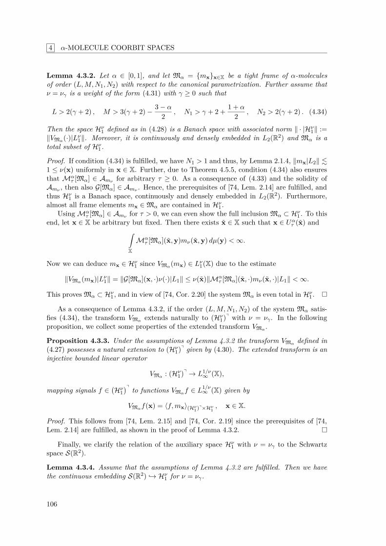
4 α-MOLECULE COORBIT SPACES
Lemma 4.3.2. Let α ∈ [0, 1], and let Mα = mxx∈X be a tight frame of α-moleculesof order (L,M,N1, N2) with respect to the canonical parametrization. Further assume thatν = νγ is a weight of the form (4.31) with γ ≥ 0 such that
L > 2(γ + 2) , M > 3(γ + 2) − 3 − α
2 , N1 > γ + 2 + 1 + α
2 , N2 > 2(γ + 2) . (4.34)
Then the space Hν1 defined as in (4.28) is a Banach space with associated norm ∥ · |Hν
1∥ :=∥VMα(·)|Lν
1∥. Moreover, it is continuously and densely embedded in L2(R2) and Mα is atotal subset of Hν
1 .
Proof. If condition (4.34) is fulfilled, we have N1 > 1 and thus, by Lemma 2.1.4, ∥mx|L2∥ .1 ≤ ν(x) uniformly in x ∈ X. Further, due to Theorem 4.5.5, condition (4.34) also ensuresthat Mα
τ [Mα] ∈ Amν for arbitrary τ ≥ 0. As a consequence of (4.33) and the solidity ofAmν , then also G[Mα] ∈ Amν . Hence, the prerequisites of [74, Lem. 2.14] are fulfilled, andthus Hν
1 is a Banach space, continuously and densely embedded in L2(R2). Furthermore,almost all frame elements mx ∈ Mα are contained in Hν
1 .Using Mα
τ [Mα] ∈ Amν for τ > 0, we can even show the full inclusion Mα ⊂ Hν1 . To this
end, let x ∈ X be arbitrary but fixed. Then there exists x ∈ X such that x ∈ Uατ (x) and
X
Mατ [Mα](x,y)mν(x,y) dµ(y) < ∞.
Now we can deduce mx ∈ Hν1 since VMα(mx) ∈ Lν
1(X) due to the estimate
∥VMα(mx)|Lν1∥ = ∥G[Mα](x, ·)ν(·)|L1∥ ≤ ν(x)∥Mα
τ [Mα](x, ·)mν(x, ·)|L1∥ < ∞.
This proves Mα ⊂ Hν1 , and in view of [74, Cor. 2.20] the system Mα is even total in Hν
1 .
As a consequence of Lemma 4.3.2, if the order (L,M,N1, N2) of the system Mα satis-fies (4.34), the transform VMα extends naturally to (Hν
1)q with ν = νγ . In the followingproposition, we collect some properties of the extended transform VMα .
Proposition 4.3.3. Under the assumptions of Lemma 4.3.2 the transform VMα defined in(4.27) possesses a natural extension to (Hν
1)q given by (4.30). The extended transform is aninjective bounded linear operator
VMα : (Hν1)q → L1/ν
∞ (X),
mapping signals f ∈Hν
1q to functions VMαf ∈ L
1/ν∞ (X) given by
VMαf(x) = ⟨f,mx⟩(Hν1 )q×Hν
1, x ∈ X.
Proof. This follows from [74, Lem. 2.15] and [74, Cor. 2.19] since the prerequisites of [74,Lem. 2.14] are fulfilled, as shown in the proof of Lemma 4.3.2.
Finally, we clarify the relation of the auxiliary space Hν1 with ν = νγ to the Schwartz
space S(R2).
Lemma 4.3.4. Assume that the assumptions of Lemma 4.3.2 are fulfilled. Then we havethe continuous embedding S(R2) → Hν
1 for ν = νγ.
106
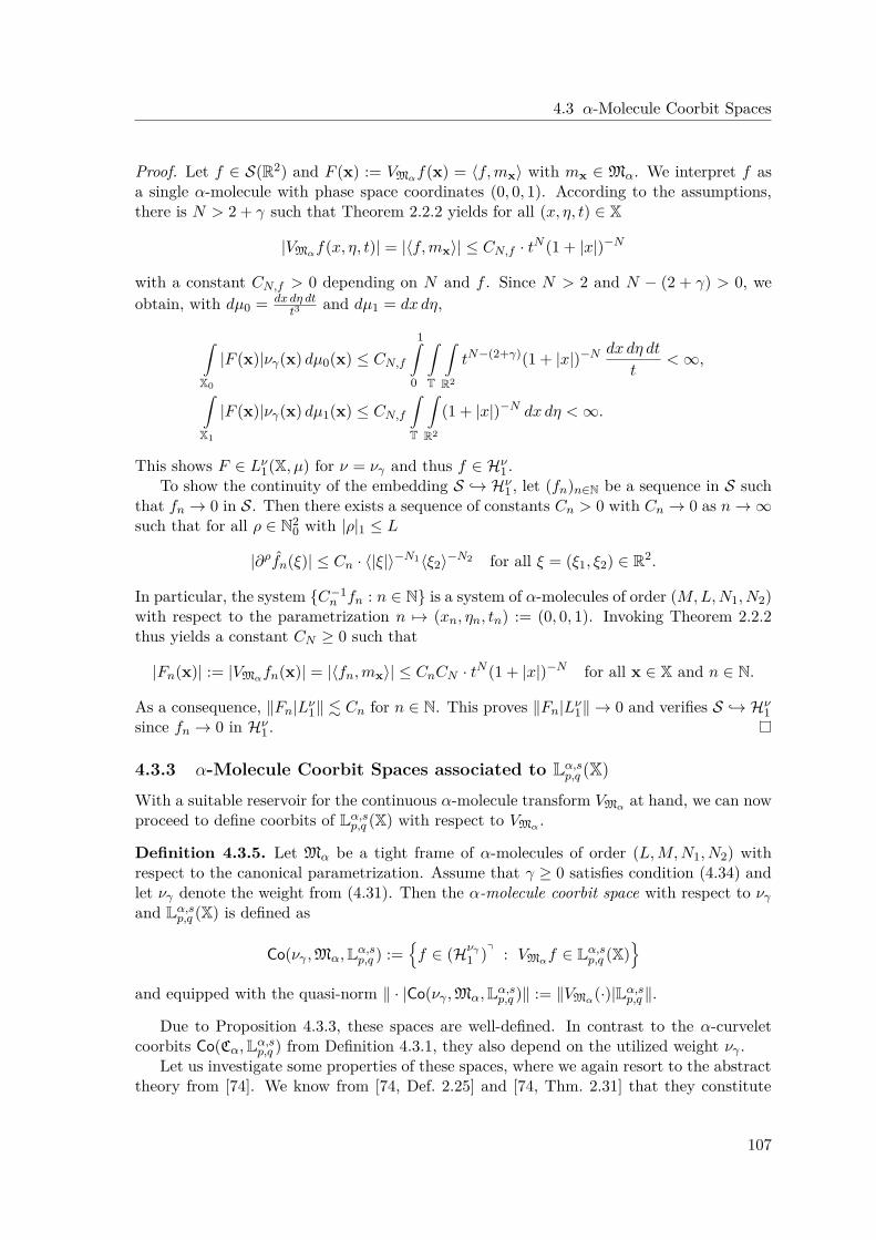
4.3 α-Molecule Coorbit Spaces
Proof. Let f ∈ S(R2) and F (x) := VMαf(x) = ⟨f,mx⟩ with mx ∈ Mα. We interpret f asa single α-molecule with phase space coordinates (0, 0, 1). According to the assumptions,there is N > 2 + γ such that Theorem 2.2.2 yields for all (x, η, t) ∈ X
|VMαf(x, η, t)| = |⟨f,mx⟩| ≤ CN,f · tN (1 + |x|)−N
with a constant CN,f > 0 depending on N and f . Since N > 2 and N − (2 + γ) > 0, weobtain, with dµ0 = dx dη dt
t3 and dµ1 = dx dη,
X0
|F (x)|νγ(x) dµ0(x) ≤ CN,f
10
T
R2
tN−(2+γ)(1 + |x|)−N dx dη dt
t< ∞,
X1
|F (x)|νγ(x) dµ1(x) ≤ CN,f
T
R2
(1 + |x|)−N dx dη < ∞.
This shows F ∈ Lν1(X, µ) for ν = νγ and thus f ∈ Hν
1 .To show the continuity of the embedding S → Hν
1 , let (fn)n∈N be a sequence in S suchthat fn → 0 in S. Then there exists a sequence of constants Cn > 0 with Cn → 0 as n → ∞such that for all ρ ∈ N2
0 with |ρ|1 ≤ L
|∂ρfn(ξ)| ≤ Cn · ⟨|ξ|⟩−N1⟨ξ2⟩−N2 for all ξ = (ξ1, ξ2) ∈ R2.
In particular, the system C−1n fn : n ∈ N is a system of α-molecules of order (M,L,N1, N2)
with respect to the parametrization n →→ (xn, ηn, tn) := (0, 0, 1). Invoking Theorem 2.2.2thus yields a constant CN ≥ 0 such that
|Fn(x)| := |VMαfn(x)| = |⟨fn,mx⟩| ≤ CnCN · tN (1 + |x|)−N for all x ∈ X and n ∈ N.
As a consequence, ∥Fn|Lν1∥ . Cn for n ∈ N. This proves ∥Fn|Lν
1∥ → 0 and verifies S → Hν1
since fn → 0 in Hν1 .
4.3.3 α-Molecule Coorbit Spaces associated to Lα,sp,q (X)
With a suitable reservoir for the continuous α-molecule transform VMα at hand, we can nowproceed to define coorbits of Lα,s
p,q (X) with respect to VMα .
Definition 4.3.5. Let Mα be a tight frame of α-molecules of order (L,M,N1, N2) withrespect to the canonical parametrization. Assume that γ ≥ 0 satisfies condition (4.34) andlet νγ denote the weight from (4.31). Then the α-molecule coorbit space with respect to νγ
and Lα,sp,q (X) is defined as
Co(νγ ,Mα,Lα,sp,q ) :=
f ∈ (Hνγ
1 )q : VMαf ∈ Lα,sp,q (X)
and equipped with the quasi-norm ∥ · |Co(νγ ,Mα,Lα,s
p,q )∥ := ∥VMα(·)|Lα,sp,q ∥.
Due to Proposition 4.3.3, these spaces are well-defined. In contrast to the α-curveletcoorbits Co(Cα,Lα,s
p,q ) from Definition 4.3.1, they also depend on the utilized weight νγ .Let us investigate some properties of these spaces, where we again resort to the abstract
theory from [74]. We know from [74, Def. 2.25] and [74, Thm. 2.31] that they constitute
107
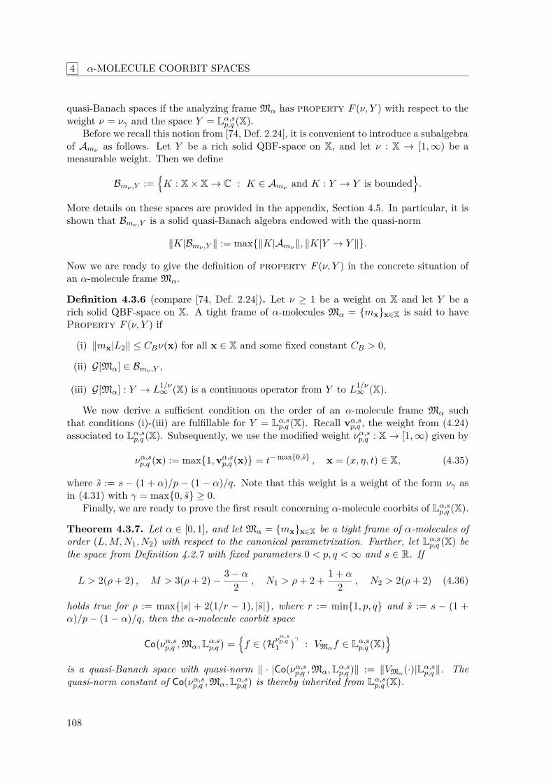
4 α-MOLECULE COORBIT SPACES
quasi-Banach spaces if the analyzing frame Mα has property F (ν, Y ) with respect to theweight ν = νγ and the space Y = Lα,s
p,q (X).Before we recall this notion from [74, Def. 2.24], it is convenient to introduce a subalgebra
of Amν as follows. Let Y be a rich solid QBF-space on X, and let ν : X → [1,∞) be ameasurable weight. Then we define
Bmν ,Y :=K : X × X → C : K ∈ Amν and K : Y → Y is bounded
.
More details on these spaces are provided in the appendix, Section 4.5. In particular, it isshown that Bmν ,Y is a solid quasi-Banach algebra endowed with the quasi-norm
∥K|Bmν ,Y ∥ := max∥K|Amν ∥, ∥K|Y → Y ∥.
Now we are ready to give the definition of property F (ν, Y ) in the concrete situation ofan α-molecule frame Mα.
Definition 4.3.6 (compare [74, Def. 2.24]). Let ν ≥ 1 be a weight on X and let Y be arich solid QBF-space on X. A tight frame of α-molecules Mα = mxx∈X is said to haveProperty F (ν, Y ) if
(i) ∥mx|L2∥ ≤ CBν(x) for all x ∈ X and some fixed constant CB > 0,
(ii) G[Mα] ∈ Bmν ,Y ,
(iii) G[Mα] : Y → L1/ν∞ (X) is a continuous operator from Y to L1/ν
∞ (X).
We now derive a sufficient condition on the order of an α-molecule frame Mα suchthat conditions (i)-(iii) are fulfillable for Y = Lα,s
p,q (X). Recall vα,sp,q , the weight from (4.24)
associated to Lα,sp,q (X). Subsequently, we use the modified weight να,s
p,q : X → [1,∞) given by
να,sp,q (x) := max1,vα,s
p,q (x) = t− max0,s , x = (x, η, t) ∈ X, (4.35)
where s := s − (1 + α)/p − (1 − α)/q. Note that this weight is a weight of the form νγ asin (4.31) with γ = max0, s ≥ 0.
Finally, we are ready to prove the first result concerning α-molecule coorbits of Lα,sp,q (X).
Theorem 4.3.7. Let α ∈ [0, 1], and let Mα = mxx∈X be a tight frame of α-molecules oforder (L,M,N1, N2) with respect to the canonical parametrization. Further, let Lα,s
p,q (X) bethe space from Definition 4.2.7 with fixed parameters 0 < p, q < ∞ and s ∈ R. If
L > 2(ρ+ 2) , M > 3(ρ+ 2) − 3 − α
2 , N1 > ρ+ 2 + 1 + α
2 , N2 > 2(ρ+ 2) (4.36)
holds true for ρ := max|s| + 2(1/r − 1), |s|, where r := min1, p, q and s := s − (1 +α)/p− (1 − α)/q, then the α-molecule coorbit space
Coνα,s
p,q ,Mα,Lα,sp,q
=f ∈ (Hνα,s
p,q
1 )q : VMαf ∈ Lα,sp,q (X)
is a quasi-Banach space with quasi-norm ∥ · |Co(να,s
p,q ,Mα,Lα,sp,q )∥ := ∥VMα(·)|Lα,s
p,q ∥. Thequasi-norm constant of Co(να,s
p,q ,Mα,Lα,sp,q ) is thereby inherited from Lα,s
p,q (X).
108
4.3 α-Molecule Coorbit Spaces
Proof. Let us assume that the order of the α-molecule frame Mα fulfills condition (4.36).We will show that under this assumption Mα has Property F (ν, Y ) as introduced inDefinition 4.3.6 for the choice ν := να,s
p,q and Y := Lα,sp,q . An application of [74, Thm. 2.31]
thus finishes the proof.It remains to verify conditions (i)-(iii) in Definition 4.3.6. Since N1 > 1 we have
∥mx|L2∥ . ν(x) for all x ∈ X by Lemma 2.1.4, proving (i). Further, as a consequenceof Theorem 4.5.5, condition (ii) holds true, namely G[Mα] ∈ Bmν ,Y which entails thatG[Mα] : Y → Y is a bounded linear operator. As a consequence of the embedding Y → L
1/ν∞ ,
this also implies that the operation G[Mα] : Y → L1/ν∞ is well-defined and continuous. Hence,
also condition (iii) is true.
An important feature of the theory of α-molecules is the transfer principle, alreadyencountered in Theorem 2.3.6 of Section 2.3 in a discrete setup. It allows to transfer certainproperties between α-molecule systems via the concept of sparsity equivalence.
The next result, Theorem 4.3.8, can be interpreted as another occurrence of the trans-fer principle, this time in a continuous setting. It relates the α-molecule coorbit spacesCo(να,s
p,q ,Mα,Lα,sp,q ) to the α-curvelet coorbits from Definition 4.3.1. Its proof is based on
Theorem 4.5.5(ii) and the abstract result [74, Lem. 2.28].
Theorem 4.3.8. For every tight frame of α-molecules Mα subject to the assumptions ofTheorem 4.3.7 we have the identification
Co(να,sp,q ,Mα,Lα,s
p,q ) ≍ Co(Cα,Lα,sp,q )
in the sense of equivalent quasi-norms.
Proof. First of all note that the α-curvelet frame Cα is a concrete instance of an α-moleculeframe satisfying the assumptions of Theorem 4.3.7. Hence, the coorbit Co(να,s
p,q ,Cα,Lα,sp,q ) is
a well-defined quasi-Banach space. Further, we have shown in Lemma 4.3.4 that S → Hν1
for ν := να,sp,q and, according to Proposition 4.1.5, the reproducing formula of VCα extends to
S ′. Hence, all prerequisites to apply [74, Lem. 2.28] in our concrete situation are fulfilled.We obtain
Co(Cα,Lα,sp,q ) ≍ Co(να,s
p,q ,Cα,Lα,sp,q ).
Let us now turn to a general α-molecule frame Mα subject to the assumptions ofTheorem 4.3.7. It follows from Theorem 4.5.5 that the cross-Gramian maximal kernelsMα
τ [Cα,Mα] and Mατ [Mα,Cα] (see (4.32) for definition) both belong to Bmν ,Y with Y :=
Lα,sp,q and ν := να,s
p,q . As a consequence of the solidity of Bmν ,Y (see Proposition 4.5.4), inparticular G[Cα,Mα] ∈ Bmν ,Y and G[Mα,Cα] ∈ Bmν ,Y hold true. With [74, Lem. 2.29] wecan therefore deduce
Co(να,sp,q ,Cα,Lα,s
p,q ) ≍ Co(να,sp,q ,Mα,Lα,s
p,q ).
Theorem 4.3.8 is a powerful tool for the analysis of Co(Cα,Lα,sp,q ). As an immediate
consequence, for example, we obtain in conjunction with Theorem 4.3.7 that Co(Cα,Lα,sp,q ) is
a quasi-Banach space with the same quasi-norm constant as Lα,sp,q (X). In the next subsection,
we will further use this theorem to deduce a discrete characterization of Co(Cα,Lα,sp,q ). The
obtained discrete description in Theorem 4.3.13 will then allow us to identify Co(Cα,Lα,sp,q )
with the shearlet smoothness spaces from [85].
109
4 α-MOLECULE COORBIT SPACES
4.3.4 Characterization via Discrete α-Curvelets
In this subsection, we will apply Theorem 4.3.8 for a special choice of Mα leading to adiscrete characterization of Co(Cα,Lα,s
p,q ). This will in particular relate these coorbit spacesto familiar scales of smoothness spaces considered for example in [85].
Let us first recall the discrete Parseval frame of α-curvelets C•α from Definition 3.2.6
indexed by the discrete α-curvelet index set
M = J × Z2. (4.37)
Hereby J = J = (j, ℓ) : j ∈ N0, ℓ ∈ Lj is a collection of scale-angle pairs with Lj :=0, 1, . . . , Lj − 1 and Lj := 2⌊j(1−α)⌋ for j ∈ N0. The system C•
α has the form
C•α = ψµµ∈M =
ψj,ℓ,k : j ∈ N0, ℓ ∈ Lj , k ∈ Z2
and consists of band-limited α-curvelets ψµ = ψj,ℓ,k ∈ L2(R2). It is useful to distinguish thecoarse-scale elements from the high-scale functions, corresponding to respective index sets
M1 := J1 × Z2 with J1 := (0, 0),and M0 := J0 × Z2 with J0 := J = (j, ℓ) : j ∈ N, ℓ ∈ Lj.
It was shown in Lemma 3.2.7 that C•α constitutes a Parseval frame for L2(R2). Moreover,
according to Proposition 3.2.8, it is a system of α-molecules of order (∞,∞,∞,∞) withrespect to the specific α-curvelet parametrization (3.28), namely (M,ΦM ) with
ΦM : M → P : (j, ℓ, k) →→ (xj,ℓ,k, ℓωj , 2−j) =R−1
ℓωjA−1
α,2jk, ℓωj , 2−j,where ωj := 2−⌊j(1−α)⌋π. For convenience, we will subsequently use the abbreviationsRj,ℓ := Rℓωj
and Aj := Aα,2j as in (3.24).Recall the subsets Uα
τ (x) of X defined in (4.15) in Section 4.2. For µ = (j, ℓ, k) ∈ Mand τ > 0, let us now define the sets
Uα,τµ := Uα,τ
j,ℓ,k := Uατ (xj,ℓ,k) with xj,ℓ,k := xµ := ΦM (µ).
More concretely, those sets can be written in the form
Uα,τj,ℓ,k = Qα,τ
j,ℓ,k × Iα,τj,ℓ × Jτ
j , (4.38)
where, with Qτ := [−τ, τ ]2, Iτ := [−τ, τ ], and Jτ := [2−τ , 2τ ],
Qα,τj,ℓ,k := xj,ℓ,k +R−1
j,ℓA−1j Qτ , Iα,τ
j,ℓ :=ℓωj + 2−j(1−α)Iτ
2π, Jτ
j :=
2−jJτ ∩ (0, 1) , j ∈ N,1 , j = 0.
For the choice τ = 13 the collection Uα,τ
µ µ∈M consists of pairwise disjoint subsets of X.
We now put Uµ := Uα, 1
3µ and introduce the positive weights
wµ :=X
XUµ(x) dµ(x) > 0. (4.39)
110
4.3 α-Molecule Coorbit Spaces
Then we define
C•α :=
ψx
x∈X where
ψx,η,t := ψµω− 1
2µ , (x, η, t) ∈ Uµ,
ψx,η,t := 0 , else.
We call C•α the continuization of the discrete α-curvelet frame C•
α.
Lemma 4.3.9. The system C•α = ψxx∈X is a continuous Parseval frame of α-molecules
of order (∞,∞,∞,∞) with respect to the canonical parametrization.
Proof. The system C•α = ψxx∈X inherits the Parseval property from C•
α = ψµµ∈M .Indeed, for every f ∈ L2(R2) we have
X
|⟨f, ψx⟩|2 dµ(x) =
µ∈M
Uµ
|⟨f, ψµ⟩|2w−1µ dµ(x) =
µ∈M
|⟨f, ψµ⟩|2 = ∥f |L2∥2.
For the verification of the α-molecule property of C•α, we define for (x, η, t) ∈ X
hx,η,t := t(1+α)/2ψx,η,tR−1
η Aα,t · +x
such that ψx,η,t = t−(1+α)/2hx,η,tA−1
α,tRη(· − x).
To finish the proof, it remains to show condition (2.5) for the functions hx,η,t.We first recall that, according to (3.26), every α-curvelet ψj,ℓ,k ∈ C•
α has the form
ψj,ℓ,k = 2j(1+α)/2ajAjRj,ℓ · −k
with a generator aj ∈ L2(R2) given by (3.25).
Hence, in case (x, η, t) ∈ Uµ for some µ = (j, ℓ, k) ∈ M , we can deduce
hx,η,t = t(1+α)/2ψx,η,tR−1
η Aα,t · +x
= ω− 1
2µ (t2j)(1+α)/2aj
AjRj,ℓR
−1η Aα,t · +(AjRj,ℓx− k)
.
Altogether, since ψx,η,t = 0 if (x, η, t) /∈ Uµ for every µ ∈ M , we obtain the spatial repre-sentation
hx,η,t =
ω− 1
2µ (∆t)(1+α)/2aj
T−T
η,t · +∆k, if (x, η, t) ∈ Uµ,
0 , else,
where we abbreviate ∆t := t2j , ∆k := AjRj,ℓx− k, and
Tη,t := A−1j Rj,ℓR
−1η A−1
α,t =:t11 t12t21 t22
.
On the Fourier side, we get
hx,η,t =
ω− 1
2µ (∆t)−(1+α)/2aj
Tη,t ·
exp
2πi⟨∆k, Tη,t·⟩
, if (x, η, t) ∈ Uµ,
0 , else.
111
4 α-MOLECULE COORBIT SPACES
Our first goal is now to show that for every fixed ρ = (ρ1, ρ2) ∈ N20
supξ∈R2
|∂ρhx,η,t(ξ)| . 1 uniformly in (x, η, t) ∈ X. (4.40)
Note that since hx,η,t ∈ C∞(R2) the derivatives ∂ρhx,η,t are well-defined. With the chainrule, we calculate for ξ ∈ R2
∂1aj(Tη,t·)
(ξ) = t11
∂1aj
(Tη,tξ) + t21
∂2aj
(Tη,tξ),
∂2aj(Tη,t·)
(ξ) = t12
∂1aj
(Tη,tξ) + t22
∂2aj
(Tη,tξ).
By iteration, we obtain for ρ = (ρ1, ρ2) ∈ N20 the expansion
∂ρ11 ∂ρ2
2aj(Tη,t·)
(ξ) =
ρ1a=0
ρ2b=0
na,bSa,b(ξ; η, t)
with combinatorial coefficients na,b ∈ N and terms Sa,b(ξ; η, t) of the form
Sa,b(ξ; η, t) :=t11at21ρ1−a
t12bt22ρ2−b
∂a+b1 ∂ρ1+ρ2−a−b
2 aj(Tη,tξ).
To estimate these terms, note that Tη,t is a matrix of the type investigated in Lemma 2.2.18and Corollary 2.2.19. With the notation there, we have
T−Tη,t = AjRj,ℓR
−1η Aα,t = T (ℓωj , 2−j , η, t).
In the relevant case (x, η, t) ∈ Uµ, it holds max∆t, (∆t)−1 ≤ 2τ and dS(ℓωj , η) ≤ τ2−j(1−α)
for τ = 13 . Hence, we can apply Lemma 2.2.18 and obtain that the entries of T−T
η,t and T Tη,t
are uniformly bounded. As a consequence, also the entries t11, t12, t21, and t22 of Tη,t areuniformly bounded. This yields |Sa,b(ξ; η, t)| . |(∂a+b
1 ∂ρ1+ρ2−a−b2 aj)(Tη,tξ)|.
Further, we recall from the proof of Proposition 3.2.8 that, for any given ρ = (ρ1, ρ2) ∈N2
0, we have uniformly in j ∈ N0
supξ∈R2
|∂ρ11 ∂ρ2
2 aj(ξ)| . 1.
Hence, we obtain
supξ∈R2
|∂a+b
1 ∂ρ1+ρ2−a−b2 aj
(Tη,tξ)| . 1 uniformly in (x, η, t) ∈ X.
All in all, this proves |Sa,b(ξ; η, t)| . 1 and we can deduce
supξ∈R2
|∂ρ11 ∂ρ2
2aj(Tη,t·)
(ξ)| . 1 uniformly in (x, η, t) ∈ X.
For the exponential term, we note
exp2πi⟨∆k, Tη,t·⟩
= exp
2πi⟨T T
η,t(∆k), ·⟩.
Whenever (x, η, t) ∈ Uµ = Uj,ℓ,k we have x ∈ Qα, 1
3j,ℓ,k and thus
∆k = AjRj,ℓx− k = AjRj,ℓ(x− xj,ℓ,k) ∈ Q13 .
112
4.3 α-Molecule Coorbit Spaces
In other words ∥∆k∥∞ ≤ 13 . We now invoke Corollary 2.2.19 which yields ∥T T
η,t∥∞→∞ ≤2
13 (1 + 1
3) ≤ 2. Hence, we get T Tη,t(∆k) ∈ Q2 = [−2, 2]2.
For every ρ = (ρ1, ρ2) ∈ N20 with |ρ|1 ≤ L and every (x, η, t) ∈ X we thus obtain
∥∂ρ11 ∂ρ2
2 exp2πi⟨∆k, Tη,t·⟩
|L∞∥ ≤ (4π)L . 1.
Finally, we take care of the prefactor ω− 12
µ (∆t)−(1+α)/2. Clearly, 2− 13 ≤ ∆t ≤ 2
13 due to
(x, η, t) ∈ Uµ. We further have wµ ≍ 1 by Corollary 4.2.12.Taken all together, our estimates prove (4.40).Next, we analyze the support properties of the functions ∂ρhx,η,t. From the support
of the generators aj (see (3.27) and the following discussion) one can directly deduce thatthere exist constants C ≥ c > 0 such that supp a0 ⊂ [−C,C]2 and for j ≥ 1
supp aj ⊂ [−C,C]2\[−c, c] × [−2j(1−α)c, 2j(1−α)c]
.
Furthermore, we clearly have
supp ∂ρhx,η,t ⊆ supp hx,η,t = supp ajTη,t ·
.
An application of Corollary 2.2.19 yields ∥Tη,t∥∞→∞ ≤ 213 (1+ 1
3) ≤ 2 and ∥T−1η,t ∥∞→∞ ≤
213 (1 + 1
3) ≤ 2. Hence, in case (x, η, t) ∈ Uµ for µ = (j, ℓ, k) ∈ M0 with j ≥ 1, we obtain
supp ∂ρhx,η,t ⊆ [−2C, 2C]2\[− c
2 ,c2 ] × [−2j(1−α) c
2 , 2j(1−α) c
2 ]. (4.41)
If (x, η, t) ∈ Uµ for µ = (0, ℓ, k) ∈ M1 with j = 0, we necessarily have t = 1 and
supp ∂ρhx,η,1 ⊆ [−2C, 2C]2. (4.42)
The uniform boundedness of the functions ∂ρhx,η,t shown in (4.40) together with thesupport properties (4.41) and (4.42) imply condition (2.5) for ∂ρhx,η,t for arbitrary or-ders (L,M,N1, N2). This is the same argument already encountered in Propositions 3.1.3and 3.2.8. The proof is finished.
Let us remark that the utilized continuization procedure does not work in a generic α-molecule setting. In the proof of Lemma 4.3.9 we have based our arguments on the fact thatthe α-curvelets are bandlimited, a specific property stronger than the generic α-moleculedecay conditions. In a general setting, the proof would thus not go through as above.
Since C•α is a continuous Parseval frame of α-molecules with respect to the canonical
parametrization, we can now apply Theorem 4.3.8 to obtain the following result.
Lemma 4.3.10. We have the equivalence
Co(Cα,Lα,sp,q ) ≍ Co(C•
α,Lα,sp,q ) :=
f ∈ S ′(R2) : VC•
αf ∈ Lα,s
p,q (X),
where Co(C•α,Lα,s
p,q ) is equipped with the quasi-norm ∥ · |Co(C•α,Lα,s
p,q )∥ := ∥VC•α(·)|Lα,s
p,q ∥.
113
4 α-MOLECULE COORBIT SPACES
Proof. For the proof, we show
Co(Cα,Lα,sp,q ) ≍ Co(να,s
p,q ,C•α,Lα,s
p,q ) ≍ Co(C•α,Lα,s
p,q ).
Since Cα and C•α are both Parseval frames of α-molecules with respect to the canonical
parametrization, and since for both the respective order is arbitrarily large (see Proposi-tions 3.1.1 and 3.1.3 and Lemma 4.3.9), an application of Theorem 4.3.8 yields the firstequivalence
Co(Cα,Lα,sp,q ) ≍ Co(να,s
p,q ,C•α,Lα,s
p,q ).
It remains to prove the second equivalence
Co(να,sp,q ,C
•α,Lα,s
p,q ) ≍ Co(C•α,Lα,s
p,q ).
Subsequently, we argue similarly as in the proof of Theorem 4.3.8, with Cα replaced byC•
α. First of all notice that C•α = ψxx∈X ⊂ S, and hence the associated transform VC•
α
extends naturally to S ′. The identification of the spaces is then proved by applying theabstract result [74, Lem. 2.28]. For this, we need to show that the reproducing formula ofVC•
αextends to S ′, which works analogously as for Cα. In essence, we need to imitate the
arguments of Subsection 4.1.2 and in particular transfer Lemma 4.1.2.The proof of this key lemma is based on (4.9) and (4.10). Hence we need to adapt these
estimates to C•α. Concerning (4.10), we obtain analogously for ϕ ∈ S and arbitrary but
fixed N > 0
|VC•αϕ(x, η, t)| = |⟨ϕ, ψx,η,t⟩| ≤ CN,ϕ · tN (1 + |x|2)−N
with a constant CN,ϕ > 0 independent of (x, η, t) ∈ X. In view of Lemma 4.3.9, this is adirect consequence of Theorem 2.2.2.
Concerning (4.9), we first observe that an analogous estimate holds true for the discreteα-curvelets ψj,ℓ,k ∈ C•
α. There exists a constant CN > 0 such that
∥ψj,ℓ,k∥N ≤ CN 2j(1+α)/22jN (1 + |xj,ℓ,k|2)N uniformly for all (j, ℓ, k) ∈ M. (4.43)
This follows analogously as in the proof of Lemma 4.1.2. The only difference is that, insteadof the generators gt of the continuous α-curvelet frame given by (3.9), we need to use thefunctions at as in (3.25).
Now we can also show that, with a constant CN > 0,
∥ψx∥N ≤ CN t−(1+α)/2t−N (1 + |x|2)N for all x = (x, η, t) ∈ X.
Indeed, let x = (x, η, t) ∈ Uα, 1
3j,ℓ,k. Then there exist ∆t ∈ J
13 = [2− 1
3 , 213 ] and ∆k ∈ Q
13 =
[−13 ,
13 ]2 such that x = R−1
j,ℓA−1j (k + ∆k) and 2jt = ∆t. Now we use (4.43) and
1 + |xj,ℓ,k|2 = 1 + |A−1j k|2 ≤ (1 + |A−1
j (k + ∆k)|2)(1 + |A−1j ∆k|2) ≤ (1 + |x|2)(1 + |∆k|2)
to get with CN := CN 2(1+α)/6+N/3(1 +√
2/3)N as desired
∥ψx∥N = ∥ψj,ℓ,k∥N ≤ CN 2j(1+α)/22jN1 + |A−1j k|2
N ≤ CN t−(1+α)/2t−N (1 + |x|2)N .
The rest of the proof is analogous to Subsection 4.1.2.
114
4.3 α-Molecule Coorbit Spaces
Next, we introduce a scale of sequence spaces on the discrete α-curvelet index set M .
Definition 4.3.11. Let α ∈ [0, 1], s ∈ R, 0 < p, q < ∞. Further, M = J × Z2 shall be theα-curvelet index set as defined in (4.37). We then define the sequence space
ℓsp,q(M) :=
(cµ)µ∈M ⊂ C : ∥(cµ)µ|ℓsp,q∥ < ∞,
with associated quasi-norm defined for (cµ)µ = (cj,ℓ,k)j,ℓ,k by
∥(cµ)µ|ℓsp,q∥ :=
(j,ℓ)∈J2jsq
k∈Z2
|cj,ℓ,k|pq/p1/q
.
The following lemma is the final discretization step on our way to Theorem 4.3.13.
Lemma 4.3.12. Define s := s− (1 + α)/p− (1 − α)/q. Then
Co(C•α,Lα,s
p,q ) ≍ Co(C•α, ℓ
sp,q) :=
f ∈ S ′(R2) : VC•
αf ∈ ℓsp,q
,
where Co(C•α, ℓ
sp,q) is equipped with the quasi-norm ∥ · |Co(C•
α, ℓsp,q)∥ := ∥VC•
α(·)|ℓsp,q∥.
Proof. Let f ∈ S ′, and let C•α = ψµµ∈M be the discrete α-curvelet frame defined in
Definition 3.2.6. We have, with cµ := ⟨f, ψµ⟩S′×S being the curvelet coefficients,
VC•αf(x) =
µ
cµω−1/2µ X α, 1
3µ (x) , x ∈ X,
where ωµ = ωj,ℓ,k are the weights defined in (4.39). Further, the short-hand notationX α,τ
µ := X α,τj,ℓ,k := XUα,τ
j,ℓ,kfor τ > 0 is used. Recalling (4.38), namely Uα,τ
j,ℓ,k = Qα,τj,ℓ,k ×Iα,τ
j,ℓ ×Jτj ,
it is useful to decompose
X α,τj,ℓ,k(x, η, t) = χτ
j (t) · χα,τj,ℓ (η) · χα,τ
j,ℓ,k(x) , (x, η, t) ∈ X,
with χτj = XJτ
j, χα,τ
j,ℓ = XIα,τj,ℓ
, and χα,τj,ℓ,k = XQα,τ
j,ℓ,k.
Since, as a consequence of Corollary 4.2.12, we have ωµ ≍ 1 uniformly for all µ ∈ M , wecan deduce for x ∈ X
|VC•αf(x)| =
µ
|cµ|ω−1/2µ X α, 1
3µ (x) ≍
µ
|cµ|X α, 13
µ (x) .
115
4 α-MOLECULE COORBIT SPACES
For arbitrary τ > 0, we then calculate for the homogeneous component,
10
T
t−sq
j,ℓ,k
cj,ℓ,kX α,τj,ℓ,k(·, η, t)
Lp
q dη dt
t
1/q
= 1
0
T
t−sq
j,ℓ
χτj (t)χα,τ
j,ℓ (η)
k
|cj,ℓ,k|pχα,τ
j,ℓ,k
L1q/p dη dt
t
1/q
≍ 1
0
T
t−sqj,ℓ
χτj (t)χα,τ
j,ℓ (η)
k
|cj,ℓ,k|pχα,τ
j,ℓ,k
L1q/p dη dt
t
1/q
=
j,ℓ
10
T
t−sqχτj (t)χα,τ
j,ℓ (η)dη dtt
k
|cj,ℓ,k|pχα,τ
j,ℓ,k
L1q/p
1/q
≍
(j,ℓ)∈J0
2jsq
k
|cj,ℓ,k|pq/p
1/q
= ∥(cµ)µ|ℓsp,q(M0)∥,
with s = s− (1 + α)/p− (1 − α)/q and implicit constants depending on τ .Hence we deduce, with τ > 0 sufficiently large,
∥(cµ)µ|ℓsp,q(M0)∥ ≍ 1
0
T
t−sq
µ
cµX α, 13
µ
Lp
q dη dt
t
1/q
≍ ∥VC•αf |Ls
p,q(X0)∥
≤ ∥VC•αf |Lα,s
p,q (X0)∥ . 1
0
T
t−sq
µ
cµX α,τµ
Lp
q dη dt
t
1/q
≍ ∥(cµ)µ|ℓsp,q(M0)∥.
Here we used ∥VC•αf |Lα,s
p,q (X0)∥ = ∥WαVC•αf |Ls
p,q(X0)∥, where Wα = Wα1 is the α-
anisotropic Wiener maximal operator from (4.17), and that we can estimate for sufficientlylarge τ > 0,
WαVC•αf(x) ≤
µ
|cµ|ω−1/2µ WαX α, 1
3µ (x) .
µ
|cµ|X α,τµ (x) , x ∈ X.
Similarly, we argue for the inhomogeneous part. Here, for τ > 0 sufficiently large,
∥(cµ)µ|ℓsp,q(M1)∥ ≍
T
µ
cµX α, 13
µ (·, η, 1)Lp
qdη
1/q
≍ ∥VC•αf |Ls
p,q(X1)∥
≤ ∥VC•αf |Lα,s
p,q (X1)∥ .
T
µ
cµX α,τµ (·, η, 1)
Lp
qdη
1/q
≍ ∥(cµ)µ|ℓsp,q(M1)∥,
116
4.4 Discretization Theory
since for arbitrary τ > 0T
j,ℓ,k
cj,ℓ,kX α,τj,ℓ,k(·, η, 1)
Lp
qdη
1/q
=
T
j,ℓ
χτj (1)χα,τ
j,ℓ (η)
k
|cj,ℓ,k|pχα,τ
j,ℓ,k
L1q/p
dη
1/q
≍
ℓ∈L0
T
χα,τ0,ℓ (η) dη
k
|c0,ℓ,k|pχα,τ
0,ℓ,k
L1q/p
1/q
≍
ℓ∈L0
k
|c0,ℓ,k|pq/p
1/q
= ∥(cµ)µ|ℓsp,q(M1)∥.
Altogether, this proves Co(C•α,Lα,s
p,q ) ≍ Co(C•α, ℓ
sp,q).
Finally, we can formulate the main result of this subsection, Theorem 4.3.13, giving adiscrete characterization of Co(Cα,Lα,s
p,q ).
Theorem 4.3.13. It holds with s := s− (1 + α)/p− (1 − α)/q and equivalent quasi-norms
Co(Cα,Lα,sp,q ) ≍ Co(C•
α, ℓsp,q).
Proof. For the proof, we just need to combine Lemma 4.3.10 and Lemma 4.3.12,
Co(Cα,Lα,sp,q ) ≍ Co(C•
α,Lα,sp,q ) ≍ Co(C•
α, ℓsp,q).
We are now able to draw a connection between the coorbits Co(Cα,Lα,sp,q ) and other known
scales of function spaces. The discrete characterization of Theorem 4.3.13 allows to identifythem with shearlet and curvelet smoothness spaces or more general decomposition spaces(see e.g. [6]), for which equivalent discretizations have been derived. For example, theycoincide, up to equivalence of quasi-norms, with the shearlet smoothness spaces consideredin [85].
The discretization procedure presented in this subsection, based on the continuizationof a discrete frame, is more or less a hands-on technique to obtain discrete descriptions. Amore systematic approach to discretizations is developed in the next section.
4.4 Discretization Theory
As we have seen in the previous section, the coorbit spaces Co(Cα,Lα,sp,q ) coincide with the
smoothness spaces defined and analyzed in [85]. In particular, they can also be characterizedas decomposition spaces (see [6]). Both, the coorbit approach as well as the decompositionapproach, offer their own advantages. One feature of coorbit theory is the rich and powerfuldiscretization machinery it comes along with. In the following, it allows us to derive verygeneral discrete descriptions of Co(Cα,Lα,s
p,q ) (see our main Theorems 4.4.19 and 4.4.21).Let us first recall the collection Uα
τ = Uατ [X] = Uα
τ (x) : x ∈ X consisting of the setsUα
τ (x) defined in (4.15) as
Uατ (x) =
x+R−1
η Aα,tQτ
×η + t1−αIτ
2π
×tJτ ∩ (0, 1)
, x ∈ X0 ,
x+R−1η Qτ
×η + Iτ
2π
×1
, x ∈ X1 ,
(4.44)
117
4 α-MOLECULE COORBIT SPACES
where Qτ = [−τ, τ ]2, Iτ = [−τ, τ ], and Jτ = [2−τ , 2τ ]. This collection Uατ constitutes a
continuous covering of X depending on α ∈ [0, 1] and a density parameter τ > 0. Later, bysuitably sampling the transform domain X, we will extract from Uα
τ discrete coverings of X.Thereby even certain types of irregular samplings will be allowed.
By a sampling PΛ of the curvelet domain X we thereby mean a pair PΛ = (Λ,P) ofsome countable index set Λ and a map P : Λ → X. For convenience, this notation will alsobe used for the point family PΛ = xλλ∈Λ where xλ := P(λ). A sampling of X at thepoints PΛ naturally leads to the family
Uατ [PΛ] :=
Uα
τ (xλ) : λ ∈ Λ
of subsets of X, whereby α ∈ [0, 1] and τ > 0 are fixed parameters.An important concept for the discretization theory is the notion of an admissible covering
of the transform domain. Let us recall this notion [74, Def. 2.4] and extend it to admissiblecollections of subsets of X.
Definition 4.4.1. Let Λ be a countable index set. A collection U = Uλλ∈Λ of subsetsof X is called admissible if it is non-empty, locally finite and if it further has the followingproperties:
i) The sets Uλ are measurable, relatively compact, and have non-void interior;
ii) The intersection number s(U) of the collection U is finite, i.e.,
s(U) := supλ∈Λ
♯µ ∈ Λ : Uλ ∩ Uµ = ∅ < ∞ . (4.45)
Note that for a partition U the intersection number s(U) is 1.
If additionally X =
λ∈Λ Uλ is fulfilled we call U an admissible covering.We call a collection U of subsets of X relatively separated if we can partition U into
a finite number of subcollections, each of which only contains pairwise disjoint sets. Theorder of the separation is the smallest possible number of such subcollections.
Note, that admissible collections of subsets of X, due to their local finiteness, are nec-essarily countable since X is σ-compact. Further, we will see in the next lemma that acollection of sets with finite intersection number N is also relatively separated of order atmost N . The other direction of this statement is not always true. However, for collec-tions of the type Uα
τ [PΛ] the reverse implication also holds, which will be proved below inCorollary 4.4.7.
Lemma 4.4.2. Let U = Uλλ∈Λ be a collection of subsets of X. If the intersection numbers(U) defined in (4.45) is finite, then U is relatively separated.
Proof. By Zorn’s lemma we can find a maximal subcollection U1 consisting of pairwisedisjoint sets. Taking out this subfamily decreases the intersection number of the remainingfamily by at least 1. Iterating this process, we end up with a partition U =
ri=1 Ui into at
most s(U) subcollections of pairwise disjoint sets.
Next, we are going to characterize those samplings PΛ = (Λ,P) of X which lead toadmissible coverings of the form Uα
τ [PΛ].
118
4.4 Discretization Theory
4.4.1 Well-spread Families of Points in X
We make the following definition in analogy to [43, Def. 3.2], where similar notions wereintroduced on locally compact groups.
Definition 4.4.3. Let α ∈ [0, 1] and let τ > 0. A family of points PΛ = xλλ∈Λ in X iscalled (α, τ)-dense if
λ∈Λ U
ατ (xλ) = X. It is called (α, τ)-separated if Uα
τ (xλ) ∩Uατ (xµ) = ∅
for λ = µ ∈ Λ. It is called relatively α-separated if there exists τ > 0 such that PΛ is a finiteunion of (α, τ)-separated subfamilies. It is called α-well-spread if it is relatively α-separatedand if it is (α, τ)-dense for some τ > 0.
The finite union of relatively α-separated families of points is again relatively α-separated.
Remark 4.4.4. Note that every subset of X can be interpreted as a family by indexing eachelement with itself. This perspective allows to apply the notions defined for point familiesin Definition 4.4.3 to subsets of X in a canonical way.
We will later need the following intuitive fact for which we nevertheless provide a shortproof for reasons of mathematical rigor.
Lemma 4.4.5. Let PΛ be an (α, τ)-separated family of points in X, α ∈ [0, 1] and τ > 0be fixed. Then there exists an extension of PΛ to an α-well-spread family of points in X,which is still (α, τ)-separated.
Proof. The proof is based upon Zorn’s lemma. Let P(Λ) denote the sampling points of PΛinterpreted as a subset of X. Then consider the class E of all (α, τ)-separated extensions ofP(Λ), partially ordered by inclusion, whereby (α, τ)-separation shall be understood in thelight of Remark 4.4.4. The union of the points in each chain in E is again an element of theclass E, i.e., an (α, τ)-separated point set. Moreover, it majorizes the chain and hence, byZorn’s lemma, there exists a maximal element in E, which we denote by P(Λ)ext.
This subset of X is (α, τ)-separated and extends P(Λ). Moreover, P(Λ)ext is (α, σ)-dense for σ ≥ h(τ, τ), since otherwise there would be x /∈
y∈P(Λ)ext Uα
σ (y), and thusUα
τ (x) ∩
y∈P(Λ)ext Uατ (y) = ∅ by Lemma 4.2.5(v). This would be a contradiction to the
maximality of P(Λ)ext. Finally note that the set P(Λ)ext is countable since, due to theσ-compactness of X, all elements of E are countable. In particular, the index set Λ of PΛcan be extended to some countable index set Λext, and P(Λ)ext, suitably indexed by Λext,becomes an extension of the family PΛ with the desired properties.
The following result establishes a connection between the relative α-separation of pointsand the intersection number of associated α-patches. Note that the finite union of set collec-tions with finite intersection numbers need not have a finite intersection number any more.Even the union of two collections of pairwise disjoint sets can have an infinite intersectionnumber in general.
Lemma 4.4.6. Assume that PΛ is a relatively α-separated family of points in X. Then foreach τ > 0 the family Uα
τ [PΛ] has a finite intersection number, dependent on τ .
Proof. Let τ > 0 be fixed, and take an arbitrary x ∈ P(Λ), where P(Λ) – as in the proofof the previous lemma – denotes the subset of X consisting of the points contained in thefamily PΛ. For the proof we will subsequently count the number of non-trivial intersectionsthe set Uα
τ (x) has with other sets in Uατ [PΛ].
119
4 α-MOLECULE COORBIT SPACES
Since PΛ is relatively α-separated there exist σ > 0, N ∈ N, and a partition Λ =N
k=1 Λk
such that the subfamilies PΛk are (α, σ)-separated. For all y ∈ P(Λ) with y ∈ X\Uαh(τ,τ)(x)
we have Uατ (x) ∩ Uα
τ (y) = ∅ due to Lemma 4.2.5(v). Hence, it only remains to count thenumber of points in P(Λk) ∩ Uα
h(τ,τ)(x) for each k ∈ 1, . . . , N. For this, we note that allthe sets in Uα
σ [PΛk ] with centers in Uαh(τ,τ)(x) are contained in the larger set Uα
f(h(τ,τ),σ)(x),which is true due to Lemma 4.2.5(iii). The volume of this set is upper-bounded by someconstant C > 0, independent of x ∈ X, according to Corollary 4.2.12. Further, also byCorollary 4.2.12, the volumes of the sets Uα
σ (y), y ∈ P(Λ), are uniformly lower-boundedby some D > 0. Since PΛk is (α, σ)-separated, we conclude that the number of points inP(Λk) ∩ Uα
h(τ,τ)(x) is bounded by C/D for each k ∈ 1, . . . , N.
As a consequence of Lemma 4.4.2 and Lemma 4.4.6, we can formulate the following resultestablishing relations between the notions of relatively α-separated points, correspondingset collections, and finite intersection numbers.
Corollary 4.4.7. Let PΛ be a family of points in X. For arbitrary τ > 0 we have theequivalence:
i) PΛ is relatively α-separated,
ii) Uατ [PΛ] is relatively separated,
iii) Uατ [PΛ] has a finite intersection number.
Proof. We use a circle argument. Assume PΛ is relatively α-separated. Then by Lemma 4.4.6the collection Uα
τ [PΛ] has a finite intersection number. By Lemma 4.4.2 this in turn impliesthat Uα
τ [PΛ] is relatively separated. Finally, if Uατ [PΛ] is relatively separated, then there
exist N ∈ N and a partition Λ =N
k=1 Λk such that Uατ [PΛk ] consists of pairwise disjoint
sets for every k ∈ 1, . . . , N. As a consequence, the families PΛk are (α, τ)-separated, andin turn PΛ is relatively α-separated.
As a consequence, with α ∈ [0, 1] and τ > 0 fixed and PΛ being a family of points in X,we have the following equivalence:
PΛ is relatively α-separated. ⇐⇒ Uατ [PΛ] is an admissible collection.
Now we are ready to prove the close relationship between admissible coverings of the formUα
τ [PΛ] and α-well-spread point families. One should compare this result to [43, Lem. 3.3],for example.
Proposition 4.4.8. Let PΛ be a family of points in X. The collection Uατ [PΛ] is an ad-
missible covering of X if and only if PΛ is α-well-spread and (α, τ)-dense in X. Moreover,if we have an admissible covering of the form Uα
τ [PΛ] for some family PΛ in X and τ > 0,then by choosing one point in each set one obtains an α-well-spread family of points.
Proof. Assume that PΛ is α-well-spread. Then PΛ is relatively α-separated and, accordingto Lemma 4.4.6, the intersection number of Uα
τ [PΛ] remains finite for all τ > 0. Assuming,in addition, (α, τ)-density, the properties of an admissible covering are easy to establish.
Conversely, if Uατ [PΛ] is an admissible covering, then PΛ is in particular (α, τ)-dense.
Moreover, also Uατ+1[PΛ] is an admissible covering, whose intersection number N is finite.
120
4.4 Discretization Theory
By Lemma 4.4.2 we can decompose Uατ+1[PΛ] into (at most) N subfamilies Uα
τ+1[PΛk ],k ∈ 1, . . . , N, consisting of pairwise disjoint sets. A sampling Pk subordinate to Uα
τ [PΛk ]is then (α, σ)-separated for small enough σ > 0. Hence, PΛ :=
k Pk is relatively α-
separated. Moreover, for large enough ρ > 0, the sampling PΛ is also (α, ρ)-dense. Thisproves that it is α-well-spread, and thus, as a special case, also PΛ is α-well-spread.
4.4.2 Associated Sequence Spaces
Let PΛ = (Λ,P) be an α-well-spread sampling of X. Then we can use PΛ as a meansto associate sequence spaces to Ls
p,q(X) and Lα,sp,q (X). The definition and analysis of these
spaces is the topic of this subsection.Let us first introduce the abstract concept of a sequence space Y ⟨U⟩ associated to a
rich solid QBF-space Y on X and an admissible collection U = Uλλ∈Λ of subsets of X.Hereby we do not require U to be a covering as in [74, Def. 2.6].
Definition 4.4.9 (compare [74, Def. 2.6]). Let Y be a rich solid QBF-space on X and letU = Uλλ∈Λ be an admissible collection of subsets of X. The sequence space Y := Y ⟨U⟩is defined as the space
Y ⟨U⟩ :=
cλλ∈Λ ⊂ C :λ∈Λ
|cλ|XUλ∈ Y
,
equipped with the quasi-norm
∥cλ|Y ⟨U⟩∥ :=
λ∈Λ|cλ|XUλ
Y .Note that, since X is σ-compact and U is admissible, the indices Λ necessarily constitute
a countable set. Further, since the collection U is locally finite, the sum
λ∈Λ |cλ|XUλis
always well-defined in a point-wise sense.A sequence cλλ∈Λ can be viewed as a function on the index set Λ. Taking this per-
spective, the spaces Y ⟨U⟩ are function spaces on Λ. Moreover, we can think of Λ asbeing equipped with the discrete topology and the counting measure. Then the notion ofa QBF-space on Λ and the corresponding terminology are available (see [74]). For betterdistinction, we refer to the latter as quasi-Banach sequence spaces, abbreviated QBS-spaces.
The space Y ⟨U⟩ inherits many properties from Y . It was shown in [74] that it constitutesa rich solid QBS-space with the same quasi-norm constant CY as Y .
Proposition 4.4.10 ([74, Prop. 2.7]). The sequence space Y ⟨U⟩ is a rich solid QBS-spacewith the same quasi-norm constant CY as Y .
Proof. We refer to [74, Prop. 2.7].
Depending on α ∈ [0, 1] and τ > 0, we now partition X as follows. We put τ := 2π⌈2π/τ⌉,
which is an integer fraction of 2π, and define for every J = (j, ℓ) ∈ N20
Xα,τJ :=
x = (x, η, t) ∈ X : t ∈ 2−jτ [1, 2τ ) , η ∈ 2−⌈jτ(1−α)⌉ℓτ + [0, τ)
.
121
4 α-MOLECULE COORBIT SPACES
Then X =
J∈N20Xα,τ
J is a partition of X, whereby many of the sets Xα,τJ are empty. Given
a sampling P : Λ → X with λ →→ xλ, the above partition further induces a correspondingpartition of the index set Λ, namely Λ =
J∈N2
0Λα,τ
J with
Λα,τJ := Λα,τ
J [P] :=λ ∈ Λ : xλ ∈ Xα.τ
J
.
Now we are ready for the next definition.
Definition 4.4.11. Let α ∈ [0, 1], s ∈ R, 0 < p, q < ∞. Let PΛ = xλλ∈Λ be a relativelyα-separated family of points in X. We then define the sequence space
ℓα,sp,q [PΛ] :=
cλλ∈Λ :
cλλ|ℓα,sp,q [PΛ]
:=
J∈N20
λ∈Λα,1
J [P]
|vα,sp,q (xλ)cλ|p
q/p1/q< ∞
,
where vα,sp,q is the weight from (4.24) given by
vα,sp,q (x) := t−s+(1+α)/p+(1−α)/q , x = (x, η, t) ∈ X .
As a consequence of Proposition 4.4.10 and the characterization established below byTheorem 4.4.12, these spaces are rich solid QBS-spaces.
Theorem 4.4.12. Let α ∈ [0, 1] and let PΛ = xλλ∈Λ be a family of points in X which isrelatively α-separated. Assume further that s ∈ R and 0 < p, q < ∞. For every fixed τ > 0we then have the equivalence
Lsp,q(X)⟨Uα
τ [PΛ]⟩ ≍ ℓα,sp,q [PΛ].
Proof. Recall the definition of the sets Uατ (x) from (4.44), namely
Uατ (x) =
x+R−1
η Aα,tQτ
×η + t1−αIτ
2π
×tJτ ∩ (0, 1)
, x ∈ X0 ,
x+R−1η Qτ
×η + Iτ
2π
×1
, x ∈ X1 ,
where x = (x, η, t) ∈ X and Qτ = [−τ, τ ]2, Iτ = [−τ, τ ], Jτ = [2−τ , 2τ ]. For the associatedcharacteristic functions, we will subsequently use the short-hand notation X α,τ
x := XUατ (x)
as introduced in (4.21). Further, recall that one can decompose these functions in the formX α,τ
x (y, θ, u) = χα,τx,η,t(y) · χα,τ
η,t (θ) · χτt (u) with characteristic functions as in (4.22).
We will handle the proof for the homogeneous and the inhomogeneous parts of thesequence spaces separately. Accordingly, we decompose Λ = Λ0 ∪ Λ1 into
Λ0 :=λ ∈ Λ : xλ ∈ X0
and Λ1 :=
λ ∈ Λ : xλ ∈ X1
.
We further introduce the convenient notation
∥cλλ∥(τ)hom := ∥cλλ∈Λ0
(Lsp,q)⟨Uα
τ [PΛ0 ]⟩ , ∥cλλ∥(τ)
in := ∥cλλ∈Λ1
(Lsp,q)⟨Uα
τ [PΛ1 ]⟩.
122
4.4 Discretization Theory
Since the intersection number of Uατ [PΛ0 ] is finite, we can rewrite the homogeneous part
of the quasi-norm in the form
∥cλλ∥(τ)hom =
10
2π0
u−sq
λ∈Λ0
|cλ|X α,τxλ
(·, θ, u)Lp
q dθ du
u
1/q
≍ 1
0
2π0
u−sq
λ∈Λ0
|cλ|pχτtλ
(u)χα,τηλ,tλ
(θ)χα,τ
xλ,ηλ,tλ
L1q/p dθ du
u
1/q
≍ 1
0
2π0
u−sq
J∈N×N0
2−jσ(1+α) λ∈Λα,σ
J
|cλ|pχτtλ
(u)χα,τηλ,tλ
(θ)
(∗)
q/p dθ du
u
1/q
,
(4.46)
where we used that for every fixed τ > 0χα,τx,η,t
L1 ≍ |Aα,tQ
τ | ≍ t1+α holds uniformly in (x, η, t) ∈ X .
We next estimate (∗) from above and below.First, we note that for λ ∈ Λα,σ
J and J = (j, ℓ) ∈ N20 we have by definition
tλ ∈ 2−jσ[1, 2σ) and ηλ ∈ 2−⌈jσ(1−α)⌉(ℓσ + [0, σ)),
where σ := 2π⌈2π/σ⌉. We deduce
tλJτ ⊆ 2−jσ[2−τ , 2τ+σ) and t1−α
λ Iτ ⊆ 2−jσ(1−α)2σ(1−α)Iτ ,
which yieldstλJ
τ ∩ (0, 1] ⊆ J+,τ,σj := 2−jσ[2−τ , 2τ+σ) ∩ (0, 1].
Further, since 2−⌈jσ(1−α)⌉ ≤ 2−jσ(1−α) and σ ≤ σ, it holds
ηλ ∈ 2−⌈jσ(1−α)⌉(ℓσ + [0, σ)) ⊆ 2−⌈jσ(1−α)⌉ℓσ + 2−jσ(1−α)[0, σ].
This implies
ηλ + t1−αλ Iτ ⊆ 2−⌈jσ(1−α)⌉ℓσ + 2−jσ(1−α)2σ(1−α)[−τ, τ ] + [0, σ]
⊆ 2−⌈jσ(1−α)⌉ℓσ + 2−jσ(1−α)2σ(1−α)[−τ, τ + σ],
and hence
(ηλ + t1−αλ Iτ )2π ⊆ I+,τ,σ
j,ℓ :=2−⌈jσ(1−α)⌉ℓσ + 2−(j−1)σ(1−α)[−τ, τ + σ]
2π.
Altogether, this proves for every J ∈ N20 and (θ, u) ∈ T × (0, 1] the inequality
λ∈Λα,σJ
|cλ|pχτtλ
(u)χα,τηλ,tλ
(θ) ≤
λ∈Λα,σJ
|cλ|pχ+,τ,σJ (θ, u), (4.47)
where χ+,τ,σJ is the characteristic function of the set I+,τ,σ
j,ℓ × J+,τ,σj .
123
4 α-MOLECULE COORBIT SPACES
Similarly, we obtain an estimate from below, this time with σ = τ however. It holds
λ∈Λα,σ
J
|cλ|pχσtλ
(u)χα,σηλ,tλ
(θ) ≥
λ∈Λα,σJ
|cλ|pχ−,σJ (θ, u) (4.48)
with the characteristic function χ−,σJ of the set
I−,σj,ℓ × J−,σ
j :=
2−⌈jσ(1−α)⌉ℓσ + 2−jσ(1−α)[0, σ)
2π
×2−jσ[1, 2σ) ∩ (0, 1]
.
Indeed, we see that for λ ∈ Λα,σJ and J = (j, ℓ) ∈ N2
0,
tλJσ ⊇ 2−jσ[1, 2σ) and t1−α
λ Iσ ⊇ 2−jσ(1−α)Iσ.
Further, as above,
ηλ ∈ 2−⌈jσ(1−α)⌉(ℓσ + [0, σ)) ⊆ 2−⌈jσ(1−α)⌉ℓσ + 2−jσ(1−α)[0, σ].
Hence
ηλ + t1−αλ Iσ ⊇ 2−⌈jσ(1−α)⌉ℓσ + 2−jσ(1−α)[0, σ],
and the estimate (4.48) follows.In the sequel, it is essential that the functions χ+,τ,σ
J and χ−,σJ are merely dependent on
the indices J ∈ N × N0, and not on the particular λ ∈ Λα,τJ any more. We calculate
10
2π0
χ−,σJ (θ, u)dθ du
u≍
10
2π0
χ+,τ,σJ (θ, u)dθ du
u≍ 2−jσ(1−α)
for fixed τ, σ > 0.Using (4.47) and (4.48), we can then prove
∥cλλ∥(τ)hom .
J∈N×N0
λ∈Λα,σ
J
|vα,sp,q (xλ)cλ|p
q/p1/q
. ∥cλλ∥(σ)hom, (4.49)
whereby the implicit constants are dependent on τ and σ.
124
4.4 Discretization Theory
For the first inequality, we plug (4.47) into (4.46) and obtain
∥cλλ∥(τ)hom .
10
2π0
u−sq
J∈N×N0
2−jσ(1+α)χ+,τ,σJ (θ, u)
λ∈Λα,σ
J
|cλ|pq/p dθ du
u
1/q
≍ 1
0
2π0
u−sq
J∈N×N0
2−jσ(1+α)q/pχ+,τ,σJ (θ, u)
λ∈Λα,σ
J
|cλ|pq/p dθ du
u
1/q
≍
J∈N×N0
2jσsq2−jσ(1+α)q/p 1
0
2π0
χ+,τ,σJ (θ, u)dθ du
u
λ∈Λα,σ
J
|cλ|pq/p
1/q
≍
J∈N×N0
2jσsq2−jσ(1+α)q/p2−jσ(1−α)
λ∈Λα,σJ
|cλ|pq/p
1/q
=
J∈N×N0
λ∈Λα,σ
J
2jσ(s−(1+α)/p−(1−α)/q)p|cλ|pq/p
1/q
≍
J∈N×N0
λ∈Λα,σ
J
|vα,sp,q (xλ)cλ|p
q/p1/q
.
Plugging (4.48) into (4.46), we obtain the second inequality
∥cλλ∥(σ)hom &
10
2π0
u−sq
J∈N×N0
2−jσ(1+α)χ−,σJ (θ, u)
λ∈Λα,σ
J
|cλ|pq/p dθ du
u
1/q
= 1
0
2π0
u−sq
J∈N×N0
2−jσ(1+α)q/pχ−,σJ (θ, u)
λ∈Λα,σ
J
|cλ|pq/p dθ du
u
1/q
≍
J∈N×N0
2jσsq2−jσ(1+α)q/p 1
0
2π0
χ−,σJ (θ, u)dθ du
u
λ∈Λα,σ
J
|cλ|pq/p
1/q
≍
J∈N×N0
2jσsq2−jσ(1+α)q/p2−jσ(1−α)
λ∈Λα,σJ
|cλ|pq/p
1/q
≍
J∈N×N0
λ∈Λα,σ
J
|vα,sp,q (xλ)cλ|p
q/p1/q
.
For arbitrary τ, σ > 0 we can finally deduce, using the symmetry of (4.49),
∥cλλ∥(τ)hom ≍ ∥cλλ∥(σ)
hom,
with implicit constants depending on those parameters. A similar estimate as (4.49) holdstrue for the inhomogeneous parts, as well as ∥cλλ∥(τ)
in ≍ ∥cλλ∥(σ)in .
This shows that for every τ > 0 the spaces (Lsp,q)⟨Uα
τ [PΛ]⟩ contain the same sequences.Furthermore, the quasi-norms of these spaces are all equivalent. Finally, choosing τ = σ = 1in (4.49) and the analogue for the inhomogeneous part yields the assertion.
125
4 α-MOLECULE COORBIT SPACES
For the Wiener spaces Lα,sp,q (X) we can derive the same associated sequence spaces.
Corollary 4.4.13. Under the same assumptions as in Theorem 4.4.12, we have
Lα,sp,q (X)⟨Uα
τ [PΛ]⟩ ≍ ℓα,sp,q [PΛ].
Proof. In view of Lemma 4.2.5(v) (see also (4.20)), we have with σ := h(τ, 1)
WαXUατ (xλ) ≤ XUα
σ (xλ)
for all xλ ∈ PΛ. Hence we can estimate
∥cλ|(Lsp,q)⟨Uα
τ [PΛ]⟩∥ ≤ ∥cλ|(Lα,sp,q )⟨Uα
τ [PΛ]⟩∥ = ∥
λ
|cλ|XUατ (xλ)|Lα,s
p,q ∥
≤ ∥
λ
|cλ|XUασ (xλ)|Ls
p,q∥ = ∥cλ|(Lsp,q)⟨Uα
σ [PΛ]⟩∥.
Since the quasi-norms on the left- and right-hand side are equivalent, according to Theo-rem 4.4.12, the assertion follows.
As the last result of this subsection, we prove that the definition of the spaces ℓα,sp,q [PΛ]
is rather robust with respect to the utilized sampling PΛ.
Corollary 4.4.14. Let PΛ = xλλ∈Λ be an α-well-spread family of points in X, and assumethat S : Λ → X is a sampling subject to the condition S(λ) ∈ Uα
τ (xλ) for all λ ∈ Λ, whereτ > 0 is arbitrary but fixed. Then ℓα,s
p,q [PΛ] ≍ ℓα,sp,q [SΛ].
Proof. Using Lemma 4.2.5(iii) and (iv), we obtain
Uατ (xλ) ⊆ Uα
σ (S(λ)) ⊆ Uατ ′(xλ)
with σ := g(τ, τ) and τ ′ := f(τ, σ). With the help of Theorem 4.4.12, we then deduce
ℓα,sp,q [PΛ] ≍
Ls
p,q(X)⟨Uα
τ [PΛ]⟩ .Ls
p,q(X)⟨Uα
σ [SΛ]⟩ ≍ ℓα,sp,q [SΛ],
and the opposite direction
ℓα,sp,q [SΛ] ≍
Ls
p,q(X)⟨Uα
σ [SΛ]⟩ .Ls
p,q(X)⟨Uα
τ ′ [PΛ]⟩ ≍ ℓα,sp,q [PΛ].
The proof is finished.
4.4.3 Discrete Characterizations: Atomic Decompositions andQuasi-Banach Frames
In this subsection we will finally apply the abstract discretization results [74, Thm. 2.48] and[74, Thm. 2.50] to our specific coorbit space setting, leading to Theorems 4.4.19 and 4.4.21below. In order to do this we need some preparation. Let us start with some definitions.
Definition 4.4.15 (compare [110, Def. 3.9]). Suppose Y is a quasi-Banach space. A familyhλλ∈Λ of bounded linear functionals on Y is called a quasi-Banach frame for Y , if thereexists a QBS-space Y = Y (Λ) and a bounded linear reconstruction operator Ω : Y → Ysuch that the following holds true,
126
4.4 Discretization Theory
i) The associated analysis operator H : f →→ hλ(f)λ∈Λ is bounded from Y to Y ,
ii) It holds Ω(H(f)) = f for all f ∈ Y .
Note that if hλλ∈Λ is a quasi-Banach frame for Y , then there exist frame bounds0 < C1 ≤ C2 ≤ ∞ such that
C1∥f |Y ∥ ≤ ∥H(f)|Y ∥ ≤ C2∥f |Y ∥.
A somewhat dual notion to a frame is the notion of an atomic decomposition.
Definition 4.4.16 (compare [110, Def. 3.8]). A family gλλ∈Λ in a quasi-Banach space Yis called an atomic decomposition for Y , if there exists a quasi-Banach frame hλλ∈Λ forY with associated QBS-space Y such that:
i) The associated synthesis operator Ω : cλλ∈Λ →→
λ∈Λcλgλ is bounded from Y to Y ,
ii) The reconstruction formula f =
λ∈Λhλ(f)gλ holds true for all f ∈ Y .
Frame Sampling
Our first discretization result, Theorem 4.4.19, yields atomic decompositions and discretequasi-Banach frames for the coorbit space Co(Cα,Lα,s
p,q ) by suitably sampling the continuousα-curvelet frame Cα. Its proof is based on the analysis of the so-called oscillation kernelassociated to Cα.
Definition 4.4.17 ([74]). Let U = Uλλ∈Λ be an admissible covering of X and let Γ :X × X → S1 be a phase function. We define the oscillation kernel associated to U and theα-curvelet frame Cα = ψxx∈X from Section 3.1 by
oscU ,Γ(x,y) := supz∈Uy
|G[Cα](x,y) − Γ(y, z)G[Cα](x, z)| = supz∈Uy
|⟨ψx, ψy − Γ(y, z)ψz⟩|,
where x,y ∈ X and Uy :=
λ:y∈UλUλ. Further, we put osc∗
U ,Γ(x,y) := oscU ,Γ(y,x).
We next want to apply [74, Thm. 2.48]. For this, we need to verify Property D(δ, ν, Y )for Cα. The following definition is in line with [74, Def. 2.43].
Definition 4.4.18 (compare [74, Def. 2.43]). Let Y be a rich solid QBF-space on X andlet Cα be the Parseval frame of α-curvelets from Section 3.1. We say that Cα possessesProperty D(δ, ν, Y ) for a weight ν ≥ 1 and some δ > 0 if it has Property F (ν, Y )(seeDefinition 4.3.6) and if there exists an admissible covering U and a phase function Γ :X ×X → S1 so that
(i) |G[Cα]|, oscU ,Γ, osc∗U ,Γ ∈ Bmν ,Y .
(ii) ∥oscU ,Γ|Bmν ,Y ∥ < δ and ∥osc∗U ,Γ|Bmν ,Y ∥ < δ.
Now we are ready to apply [74, Thm. 2.48]. We obtain the theorem below.
127
4 α-MOLECULE COORBIT SPACES
Theorem 4.4.19. Let α ∈ [0, 1] and let Cα := ψxx∈X be the continuous Parseval frameof α-curvelets constructed in Section 3.1. Further, let s ∈ R and 0 < p, q < ∞ be fixed.Then there exists τ0 = τ0[α, s, p, q] > 0 such that for every α-well-spread sampling PΛ of Xof density τ ≤ τ0 the sampled system ψλ := ψxλ
: λ ∈ Λ is a discrete α-curvelet frame forCo(Cα,Lα,s
p,q ) which possesses a corresponding dual frame ψλ : λ ∈ Λ such that:
i) (Analysis) For f ∈ (Hν1)q with ν = να,s
p,q as in (4.35) we have
f ∈ Co(Cα,Lα,sp,q ) ⇔ ⟨f, ψλ⟩λ ∈ ℓα,s
p,q [PΛ] ⇔ ⟨f, ψλ⟩λ ∈ ℓα,sp,q [PΛ].
In case f ∈ Co(Cα,Lα,sp,q ) the quasi-norms are equivalent, i.e.,
∥f |Co(Cα,Lα,sp,q )∥ ≍ ∥⟨f, ψλ⟩λ|ℓα,s
p,q [PΛ]∥ ≍ ∥⟨f, ψλ⟩λ|ℓα,sp,q [PΛ]∥ .
ii) (Synthesis) For each sequence cλλ ∈ ℓα,sp,q [PΛ] the sums
λ∈Λcλψλ and
λ∈Λ
cλψλ
converge unconditionally in Co(Cα,Lα,sp,q ). Moreover, the assigned synthesis operators
are bounded from ℓα,sp,q [PΛ] to Co(Cα,Lα,s
p,q ).
iii) (Reconstruction) For all f ∈ Co(Cα,Lα,sp,q ) we have
f =λ∈Λ
⟨f, ψλ⟩ψλ =λ∈Λ
⟨f, ψλ⟩ψλ .
Proof. We have shown in Proposition 4.2.9 that Y := Lα,sp,q is a rich solid QBF-space on
X. Let CY denote the associated quasi-norm constant and ν := να,sp,q the associated weight
defined in (4.35). We know from Proposition 3.1.3 and Theorem 4.5.5 that G[Cα] ∈ Bmν ,Y .Hence, we can choose a number δ = δ[α, s, p, q] > 0 which satisfies
δ(1 + CY )
|G[Cα]|Bmν ,Y
+ δCY
CY ≤ 1,
the condition required in [74, Thm. 2.48].Now assume that PΛ : Λ → X defines an α-well-spread and (α, τ)-dense point family
xλλ∈Λ in X. According to Proposition 4.4.8, the collection U := Uατ [PΛ] is then an
admissible covering. Further, due to Lemma 4.2.5(iv), if σ ≥ g(τ, τ) we have
Uy :=
λ:y∈Uατ (xλ)
Uατ (xλ) ⊆ Uα
σ (y) for all y ∈ X.
It follows, with Γ ≡ 1, that oscU ,Γ(x,y) ≤ oscσ(x,y) and osc∗U ,Γ(x,y) ≤ osc∗
σ(x,y), whereoscσ is the oscillation kernel from Definition 4.5.6.
According to Theorem 4.5.7, there further exists σ0 > 0 such that
∥oscσ|Bmν ,Y ∥ < δ and ∥osc∗σ|Bmν ,Y ∥ < δ for all σ ≤ σ0.
We now choose τ0 > 0 such that σ0 ≥ g(τ0, τ0). Then for all τ ≤ τ0 and U = Uατ [PΛ]
∥oscU ,Γ|Bmν ,Y ∥ < δ and ∥osc∗U ,Γ|Bmν ,Y ∥ < δ.
This shows that Cα possesses Property D(δ, ν, Y ) with respect to U = Uατ [PΛ] if τ ≤ τ0.
Hence we can apply [74, Thm. 2.48] with sampling points xλ ∈ Uλ = Uατ (xλ). Finally, note
that it holds ℓα,sp,q [PΛ] ≍ Lα,s
p,q (X)⟨Uατ [PΛ]⟩ due to Corollary 4.4.13. Taking into account
Corollary 4.2.12 and the fact that the finite sequences are dense in ℓα,sp,q [PΛ], since p, q < ∞,
the assertions follow.
128
4.4 Discretization Theory
Frame Expansion
Another useful discretization result of the abstract coorbit theory is [74, Thm. 2.50]. Sub-sequently, we consider a discrete frame M•
α = mλλ∈Λ of α-molecules, indexed by somecountable index set Λ, such that the associated parametrization Φ : Λ → X yields an α-well-spread family ΦΛ of points in X. In Theorem 4.4.21, we will derive a sufficient condition,using the abstract result [74, Thm. 2.50], when such a frame constitutes a quasi-Banachframe as well as an atomic decomposition for the coorbit Co(Cα,Lα,s
p,q ).The proof is based on the analysis of so-called cross-Gramian maximal kernels defined
as follows.
Definition 4.4.20 (compare [74, eq. (2.13)]). Let Mα = mxx∈X and Mα = mxx∈X betwo systems of α-molecules of order (L,M,N1, N2) with respect to the canonical parametriza-tion. Let U = Uλλ∈Λ be an admissible covering of X. The associated cross-Gramianmaximal kernel is defined by
MU [Mα,Mα](x,y) := supz∈Uy
|G[Mα,Mα](x, z)| = supz∈Uy
|⟨mx, mz⟩|, x,y ∈ X .
where Uy :=
λ:y∈UλUλ. Further, we put MU [Mα,Mα]∗(x,y) := MU [Mα,Mα](y,x).
Now we can formulate the next theorem and prove it with [74, Thm. 2.50] (see also[111, Thm. 3.14]). Recall that Cα = ψxx∈X denotes the continuous Parseval frame ofα-curvelets from Section 3.1.
Theorem 4.4.21. Let α ∈ [0, 1] and let M•α = mλλ∈Λ and M•
α = mλλ∈Λ be two discreteα-molecule frames in L2(R2) of order (L,M,N1, N2) and with respective parametrizationsΦ : Λ → X and Φ : Λ → X. Further, assume that M•
α and M•α are dual to each other, i.e.,
f =λ∈Λ
⟨f, mλ⟩mλ =λ∈Λ
⟨f,mλ⟩mλ for all f ∈ L2(R2). (4.50)
Provided that the following conditions are fulfilled:
i) There exist τ > 0 and an α-well-spread point family PΛ = xλλ∈Λ in X such that
Φ(λ) ∈ Uατ (xλ) and Φ(λ) ∈ Uα
τ (xλ) for all λ ∈ Λ,
ii) The order (L,M,N1, N2) of M•α and M•
α satisfies condition (4.36) with respect tos ∈ R and 0 < p, q < ∞,
then both frames M•α and M•
α are contained in Hν1 , where ν := να,s
p,q as in (4.35), and the ex-pansion (4.50) is valid for all f ∈ Co(Cα,Lα,s
p,q ) with quasi-norm convergence in Co(Cα,Lα,sp,q ).
Here ⟨·, ·⟩ must be interpreted as the duality product of the pairing (Hν1)q × Hν
1 .Furthermore, for every f ∈ (Hν
1)q we have
f ∈ Co(Cα,Lα,sp,q ) ⇔
⟨f,mλ⟩
λ
∈ ℓα,sp,q [PΛ] ⇔
⟨f, mλ⟩
λ
∈ ℓα,sp,q [PΛ] ,
and – in case f ∈ Co(Cα,Lα,sp,q ) – it holds
∥f |Co(Cα,Lα,sp,q )∥ ≍ ∥
⟨f,mλ⟩
λ|ℓα,s
p,q [PΛ]∥ ≍ ∥⟨f, mλ⟩
λ|ℓα,s
p,q [PΛ]∥ .
129
4 α-MOLECULE COORBIT SPACES
Proof. We want to apply [74, Thm. 2.50]. To this end, note that according to Lemma 4.4.6the intersection number N of Uα
τ [PΛ] is finite, where τ > 0 stems from condition (i).By Lemma 4.4.2 we can thus split the family PΛ into at most N subfamilies PΛk , wherek ∈ 1, . . . , r and r ≤ N , which are each (α, τ)-separated. The associated splitting ofthe index set Λ shall be denoted by Λk. We obtain corresponding collections Uα
τ [PΛk ],k ∈ 1, . . . , r, consisting of pairwise disjoint sets.
Next, we build r continuous families of α-molecules. We define for k ∈ 1, . . . , r:
M(k)α := m(k)
x : x ∈ X with m(k)x :=
mλ if x = Φ(λ), λ ∈ Λk,
0 else,
M(k)α := m(k)
x : x ∈ X with m(k)x :=
mλ if x = Φ(λ), λ ∈ Λk,
0 else.
By definition, these families are nonzero merely on a discrete subset of X, namely thesampling points determined by Φ and Φ. Further, they are systems of α-molecules withrespect to the canonical parametrization of the same order (L,M,N1, N2) as M•
α and M•α.
We proceed by extending each point family PΛk to an α-well-spread family Pextk that is
still (α, τ)-separated. This is possible by Lemma 4.4.5. More concretely, looking into theproof of this lemma, we can assume Pext
k to be (α, σ)-dense for some σ ≥ h(τ, τ), where his the function from Lemma 4.2.5(v).
Let us denote the extended index sets by Λextk , and for the extended point families Pext
k
let us write Pextk = xk
λ : λ ∈ Λextk with xk
λ := xλ for λ ∈ Λk. By Proposition 4.4.8, weobtain associated admissible coverings Uk := Uα
σ [Pextk ] = Uk
λ : λ ∈ Λextk where Uk
λ :=Uα
σ (xkλ). Furthermore, these coverings are moderate (see [46, page 260] for a definition)
since µ(Ukλ ) ≍ 1 by Corollary 4.2.12. In particular, [74, eq. 2.25] is satisfied.
In view of Lemma 4.2.5(iv), if ρ ≥ g(σ, σ) we have
Uky :=
λ:y∈Uk
λ
Ukλ ⊆ Uα
ρ (y) for all y ∈ X.
Hence, we can define and estimate the kernel functions Kk and Kk, k ∈ 1, . . . , r, as follows,
Kk(x,y) := MUk[M(k)
α ,Cα](x,y) ≤ Mαρ [M(k)
α ,Cα](x,y) ,Kk(x,y) := MUk
[M(k)α ,Cα](x,y) ≤ Mα
ρ [M(k)α ,Cα](x,y) ,
with Mαρ [M(k)
α ,Cα] and Mαρ [M(k)
α ,Cα] being defined as in (4.54).According to Theorem 4.5.5 and due to condition (ii), these kernel functions as well as
their involutions Mαρ [M(k)
α ,Cα]∗ and Mαρ [M(k)
α ,Cα]∗, are elements of the algebra Bmν ,Y forν := να,s
p,q and Y := Lα,sp,q . By solidity, the kernels Kk, Kk, K∗
k, and K∗k thus also belong to
Bmν ,Y .We now choose for each k ∈ 1, . . . , r and each λ ∈ Λext
k sampling points xk,λ ∈ Ukλ and
xk,λ ∈ Ukλ as follows:
xk,λ := Φ(λ) and xk,λ := Φ(λ) for λ ∈ Λk,
xk,λ := xk,λ ∈ Uατ (xk
λ) arbitrary for λ ∈ Λextk \Λk.
130
4.5 Appendix: Kernel Analysis
Then we get from (4.50) the validity of
f =r
k=1
λ∈Λext
k
⟨f, m(k)xk,λ
⟩m(k)xk,λ =
rk=1
λ∈Λext
k
⟨f,m(k)xk,λ⟩m(k)
xk,λfor all f ∈ L2(R2).
Hence, the prerequisites to apply [74, Thm. 2.50] are (almost) fulfilled, albeit not pre-cisely since we have used possibly different coverings Uk for each pair of kernels Kk and Kk.Moreover, the primal and dual sampling points xk,λ ∈ Uk
λ and xk,λ ∈ Ukλ might not coincide
and may also differ for different k.Hence, we need to apply the original theorem [74, Thm. 2.50] in a slightly generalized
form. This is possible, since revisiting the proof of [74, Thm. 2.50] (see [111, Thm. 3.14]), itbecomes clear that the statement of [74, Thm. 2.50] still holds true under these generalizedassumptions. An application thus yields the assertion. To see this, we remark that as aconsequence of Corollary 4.4.13
rk=1
∥⟨f,m(k)xk,λ⟩λ∈Λk |Lα,s
p,q (X)⟨Uk⟩∥ ≍ ∥⟨f,mλ⟩λ∈Λ|ℓα,sp,q [PΛ]∥.
Also observe that the finite sequences are dense in ℓα,sp,q [PΛ].
Note that the frames M•α and M•
α in Theorem 4.4.21 need not coincide, which extends therange of applicability of the result significantly. For example, frames of compactly supportedshearlets, where no tight frame constructions are known, might be possible choices for M•
α.A drawback for the application however is the required knowledge on the dual frame, whichis not available for many concrete constructions.
4.5 Appendix: Kernel AnalysisIn this appendix the technical details are provided needed for the application of the abstracttheory of coorbit spaces from [74] to our concrete setting of α-molecule coorbits. Theabstract theory relies heavily on the analysis of certain kernel functions and their mappingproperties. In the following exposition we pursue the required analysis for the specifickernels associated with the continuous α-molecule transform.
Thereby, in our concrete setting, a kernel function, or a kernel for short, refers to ameasurable function K : X × X → C. For convenience, we collect all such kernels in the set
K :=K : X × X → C : K (µ⊗ µ)-measurable
and identify those which coincide apart from a null set. Clearly, equipped with point-wiseaddition and scalar multiplication, K is a C-linear space. Moreover, this space is closedunder involution, i.e., the operation given by
K →→ K∗ where K∗(x,y) := K(y,x) , x,y ∈ X.
The significance of the kernel space K stems from the fact that its elements naturallyact on functions with domain X. This shall be understood in the following sense: A kernelK ∈ K maps a measurable function F : X → C to a function KF := K[F ] via
K[F ](x) :=X
K(x,y)F (y) dµ(y) , x ∈ X,
131
4 α-MOLECULE COORBIT SPACES
whenever the integral on the right-hand side is well-defined for almost every x ∈ X. Notehowever, that for a given kernel K ∈ K this may not be the case for all measurable functionsF : X → C.
The operator associated with a kernel K will sometimes be denoted by Kop, for betterdistinction, but whenever the meaning is clear we will use the same notation K. The com-position Kop Lop of two kernel operators leads to a corresponding multiplication operationon the kernel space K given by
K L
(x,y) :=
X
K(x, z)L(z,y) dµ(z) , x,y ∈ X. (4.51)
But one has to be careful since again this multiplication is not a well-defined operation forall kernel pairs (K,L) in K × K.
The algebra Amν A natural subset of K, where the multiplication is well-defined for allkernel pairs, is the space (see [46, page 249])
A :=K ∈ K : ∥K|A∥ < ∞
,
where for K ∈ K the symbol ∥K|A∥ denotes the norm
∥K|A∥ := max
ess supx∈X
y∈X
|K(x,y)| dµ(y), ess supy∈X
x∈X
|K(x,y)| dµ(x).
The space A is even a Banach algebra as we will see in Proposition 4.5.1 below. Moreover,it is solid and closed under involution. The solidity of a kernel space is thereby definedanalogously to the notion on a QBF-space, i.e., a subspace L ⊆ K with quasi-norm ∥ · |L∥is said to be solid if for every kernel K ∈ K we have the implication
|K| ≤ |L| for some L ∈ L ⇒ K ∈ L and ∥K|L∥ ≤ ∥L|L∥ .
Before we come to Proposition 4.5.1, let us introduce a more general weighted version of Awhich plays an essential role in coorbit theory.
Given a weight function ν : X → R+ on X, which is without saying always assumed tobe measurable, we can associate a bivariate weight mν : X × X → [1,∞) via
mν(x,y) := maxν(x)ν(y) ,
ν(y)ν(x)
, x,y ∈ X.
The weighted kernel algebra Amν (see [46, page 250] and [74, eq. (2.8)]) is then defined by
Amν :=K ∈ K : ∥K|Amν ∥ < ∞
with norm ∥K|Amν ∥ := ∥Kmν |A∥.
For a constant weight ν we get mν ≡ 1 and thus retrieve the unweighted algebra A = Amν .In general, we have mν ≥ 1 wherefore Amν is always continuously embedded into A.
An important structural result for Amν is stated in the following proposition.
Proposition 4.5.1. For each weight ν : X → R+ the kernel space Amν is a Banach algebra,solid, and closed under involution.
132
4.5 Appendix: Kernel Analysis
Since a proof of this fact is not contained in [46, 111, 74] we decided to include one inthis thesis.
Proof. We first prove that Amν is a Banach space with norm ∥ · |Amν ∥. Apart from thecompleteness, everything is straightforward to verify. Hence let us just concentrate on thecompleteness and consider a Cauchy sequence (Kn)n∈N in Amν .
Without loss of generality we can assume ∥Kn+1 − Kn|Amν ∥ ≤ 2−n for every n ∈ N.We then define the auxiliary kernels Lm, m ∈ N, given by
Lm(x,y) :=m
n=1|(Kn+1(x,y) −Kn(x,y))mν(x,y)| , x,y ∈ X.
Using monotone convergence, we obtain
∥ limm→∞
Lm(x, ·)|L1∥ = limm→∞
∥Lm(x, ·)|L1∥ ≤∞
n=1∥Kn+1 −Kn|Amν ∥ ≤ 1 for a.e. x ∈ X.
Hence, at every position x ∈ X apart from a null set, the sequence∞
n=1 |(Kn+1(x,y) −Kn(x,y))mν(x,y)| converges for almost all y ∈ X. Since everywhere mν(x,y) = 0, also∞
n=1 |(Kn+1(x,y) − Kn(x,y))| converges for almost all x,y ∈ X. This allows to define akernel K as the pointwise limit
K(x,y) := limn→∞
Kn(x,y) , x,y ∈ X,
since those limits exist almost everywhere. This kernel is also characterized by the property
K(x, ·)mν(x, ·) = L1- limn→∞Kn(x, ·)mν(x, ·) for a.e. x ∈ X,K(·,y)mν(·,y) = L1- limn→∞Kn(·,y)mν(·,y) for a.e. y ∈ X.
This follows from the fact that (Kn(x, ·)mν(x, ·))n∈N and (Kn(·,y)mν(·,y))n∈N are Cauchysequences in L1 for almost every x ∈ X and y ∈ X, respectively.
The validity of K ∈ Amν and Kn → K in Amν is now a consequence of the observation
ess supx∈X
∥(Kn(x, ·) −K(x, ·))mν(x, ·)|L1∥ = ess supx∈X
limm→∞
∥(Kn(x, ·) −Km(x, ·))mν(x, ·)|L1∥
≤ lim infm→∞
ess supx∈X
∥(Kn(x, ·) −Km(x, ·))mν(x, ·)|L1∥
≤ lim infm→∞
∥Kn −Km|Amν ∥ → 0 (n → ∞)
and the analogous result
ess supy∈X
∥(Kn(·,y) −K(·,y))mν(·,y)|L1∥ ≤ lim infm→∞
∥Kn −Km|Amν ∥ → 0 (n → ∞).
This proves the completeness of Amν and establishes Amν as a Banach space. The solidityof Amν and the closedness under involution are clear.
Let us finally turn to the multiplicative structure. First observe that
mν(x,y) ≤ mν(x, z)mν(z,y) for all x,y, z ∈ X.
133
4 α-MOLECULE COORBIT SPACES
Hence, we can estimate for almost every x ∈ XX
X
|K(x, z)L(z,y)|mν(x,y) dµ(z) dµ(y)
≤X
|K(x, z)|mν(x, z) X
|L(z,y)|mν(z,y) dµ(y)dµ(z)
≤ ∥L|Amν ∥X
|K(x, z)|mν(x, z) dµ(z) ≤ ∥K|Amν ∥∥L|Amν ∥.
As a consequence of this estimate and the corresponding dual resultX
X
|K(x, z)L(z,y)|mν(x,y) dµ(z) dµ(x) ≤ ∥K|Amν ∥∥L|Amν ∥,
we obtain the point-wise well-definedness of the product kernel (K L)(x,y) at almost every(x,y) ∈ X × X and the estimate
∥K L|Amν ∥ ≤ ∥K|Amν ∥∥L|Amν ∥.
The proof is finished.
Next, we are interested in mapping properties of kernels belonging to Amν . Using Schur’stest and the Riesz-Thorin theorem, it can be shown that kernels in A operate continuouslyon the Lebesgue spaces Lp(X) if 1 ≤ p ≤ ∞. More general, as observed in [46], kernels inthe weighted algebra Amν operate continuously on the weighted spaces Lν
p(X) and L1/νp (X).
Lemma 4.5.2 (see [46, page 250]). Let p ∈ [1,∞] and ν : X → R+ be a weight on X. Thenall kernels K ∈ Amν operate continuously on Lν
p(X) and L1/νp (X) with ∥Kop|Lν
p → Lνp∥ ≤
∥K|Amν ∥ and ∥Kop|L1/νp → L
1/νp ∥ ≤ ∥K|Amν ∥.
Proof. Let K := |K|mν . Then, by Schur’s test and complex interpolation, K operates con-tinuously on Lp, 1 ≤ p ≤ ∞, with ∥Kop|Lp → Lp∥ ≤ ∥K|A∥ = ∥K|Amν ∥. Further, the ker-nelsK1 andK2 defined byK1(x,y) := ν(x)K(x,y)/ν(y) andK2(x,y) := ν(y)K(x,y)/ν(x)for x,y ∈ X are majorized by K, i.e., |K1| ≤ K and |K2| ≤ K. In view of Lemma 4.5.3and the solidity of Lp, these kernels hence also induce continuous operations on Lp with∥Kop
i : Lp → Lp∥ ≤ ∥K|Amν ∥ for i = 1, 2. This translates to the assertion of the lemma.
The algebra Bmν ,Y Another way to define meaningful subspaces of the kernel space Kis to distinguish those kernels which operate continuously on some given function spaceY . To be more concrete, let us assume that Y is a QBF-space on X. The space L(Y ) ofall bounded linear operators on Y is then a quasi-Banach space with the same quasi-normconstant CY as Y . Moreover, equipped with the operator-quasi-norm and the compositionoperation as multiplication, this space becomes a quasi-Banach algebra since in particular
∥K L|Y → Y ∥ ≤ ∥K|Y → Y ∥∥L|Y → Y ∥ for every K,L ∈ L(Y ).
134
4.5 Appendix: Kernel Analysis
Also observe that, if Tn → T in L(Y ), we have limn→∞ ∥T − Tn|Y → Y ∥ = 0 and thus theestimate
C−1Y ∥T |Y → Y ∥ ≤ lim inf
n→∞
∥T − Tn|Y → Y ∥ + ∥Tn|Y → Y ∥
= lim inf
n→∞∥Tn|Y → Y ∥.
(4.52)
In case of kernel operations, things are a bit more complicated, since in general not allelements of L(Y ) stem from associated kernel functions.
A useful auxiliary result concerning the operations of kernels on solid QBF-spaces is thefollowing lemma.
Lemma 4.5.3 ([74, Lem. 2.45]). Let Y be a solid QBF-space on X, and let K : X×X → Cbe a kernel such that |K| operates continuously on Y . Further, let L : X×X → C be a kernelsatisfying |L| ≤ |K| almost everywhere. Then L acts continuously on Y with the estimate∥Lop|Y → Y ∥ ≤ ∥|K|op|Y → Y ∥.
Proof. Let F ∈ Y . Then by the solidity of Y we have |F | ∈ Y with ∥F |Y ∥ = ∥|F ||Y ∥. Itfollows |K|op[|F |] ∈ Y , and since
X|L(x,y)F (y)| dµ(y) ≤
X
|K(x,y)F (y)| dµ(y) = |K|op[|F |](x)
for almost every x ∈ X, the operator
Lop[F ](x) =XL(x,y)F (y) dµ(y)
is well-defined since the integral converges absolutely at these x ∈ X. Moreover, by solidityof Y , we have Lop[F ] ∈ Y and finally, we conclude
∥Lop[F ]|Y ∥ ≤ ∥|L|op[|F |]|Y ∥ ≤ ∥|K|op[|F |]|Y ∥ ≤ ∥|K|op|Y → Y ∥∥F |Y ∥.
Hence L defines a continuous operator Lop : Y → Y with ∥Lop|Y → Y ∥ ≤ ∥|K|op|Y →Y ∥.
For the choice L = K in Lemma 4.5.3 we can deduce that especially K acts on Y with∥Kop|Y → Y ∥ ≤ ∥|K|op|Y → Y ∥. Notice however that ∥Kop|Y → Y ∥ = ∥|K|op|Y → Y ∥need not be true.
Now we can give the definition of the algebra Bmν ,Y which plays an important role incoorbit theory. It is the space
Bmν ,Y :=K ∈ K : ∥K|Amν ∥ < ∞ , |K|op : Y → Y operates continuously
equipped with the quasi-norm
∥K|Bmν ,Y ∥ := max
∥K|Amν ∥,|K|op
Y → Y.
Note that, motivated by Lemma 4.5.3, we pursued a small modification in the definitionof Bmν ,Y compared to [74] or [111, eq. (3.4)]. We require |K|op to be a continuous operatoron Y , which is a slightly stricter condition than just requiring this for Kop. The algebraBmν ,Y is then always a solid space in the sense defined above. Moreover, this modificationleads to a straight-forward proof that Bmν ,Y is a quasi-Banach algebra.
135
4 α-MOLECULE COORBIT SPACES
Proposition 4.5.4. Let Y be a rich solid QBF-space on X and let ν : X → R+ be a weightfunction. Then Bmν ,Y is a solid quasi-Banach algebra.
Proof. It is clear that Bmν ,Y is an algebra. Further, ∥ · |Bmν ,Y ∥ is a quasi-norm on Bmν ,Y
with quasi-norm constant CY inherited from Y . The solidity of Bmν ,Y follows directly fromLemma 4.5.3 and the solidity of Amν . Further ∥K L|Bmν ,Y ∥ ≤ ∥K|Bmν ,Y ∥∥L|Bmν ,Y ∥.
It remains to prove the completeness. First note that a Cauchy sequence (Kn)n∈N inBmν ,Y is also Cauchy sequences in Amν . By Proposition 4.5.1 we hence obtain a uniquekernel K ∈ Amν as the Amν -limit. Moreover, by possibly taking a suitable subsequence,we can without loss of generality assume that Kn → K pointwise almost everywhere (seeproof of Proposition 4.5.1). In the sequel we will use this assumption.
Using the notation K0 := 0 for the zero kernel, we will subsequently show that |K−Kn|op
is a well-defined element of L(Y ) for all n ∈ N0 and that |K − Kn|op → 0 in L(Y ). Withthis we then directly obtain K ∈ Bmν ,Y and Kn → K in Bmν ,Y , finishing the proof.
Let us turn to the operator side. For each fixed n ∈ N0, the operator sequence (|Km −Kn|op)m∈N is a Cauchy sequence in L(Y ) due to the estimate ||Km −Kn| − |Km −Kn|| ≤|Km −Km|, the solidity of Y and Lemma 4.5.3. Let Kn ∈ L(Y ) denote the respective limitsand take an arbitrary F ∈ Y . Using Fatou’s lemma, we can estimate for almost every x ∈ X
X|(K −Kn)(x,y)F (y)| dµ(y) =
X
limm→∞
|(Km −Kn)(x,y)F (y)| dµ(y)
≤ lim infm→∞
X
|(Km −Kn)(x,y)F (y)| dµ(y)
= lim infm→∞
|Km −Kn|op[|F |](x) ≤ Kn[|F |](x).
Here the last inequality is due to Lemma 4.2.1.Since Kn
|F |
∈ Y , we deduce that |K − Kn|opF is well-defined pointwise almost ev-erywhere for every F ∈ Y . Further, by solidity, |K − Kn|opF ∈ Y since ||K − Kn|opF | ≤|K−Kn|op[|F |] ≤ Kn[|F |]. Moreover, the operators |K−Kn|op are contained in L(Y ) since
∥|K −Kn|opF |Y ∥ ≤ ∥Kn[|F |]|Y ∥ ≤ ∥Kn|Y → Y ∥∥F |Y ∥. (4.53)
For the particular choice n = 0, this shows |K|op ∈ L(Y ) and hence K ∈ Bmν ,Y . Further,using (4.52), we get for n ≥ 1
C−1Y ∥Kn|Y → Y ∥ ≤ lim inf
m→∞∥|Km −Kn|op|Y → Y ∥ ≤ lim inf
m→∞∥Km −Kn|Bmν ,Y ∥,
which with (4.53) finally implies
∥|K −Kn|op|Y → Y ∥ ≤ ∥Kn|Y → Y ∥ ≤ CY lim infm→∞
∥Km −Kn|Bmν ,Y ∥ → 0 (n → ∞).
Together with ∥K − Kn|Amν ∥ → 0, this establishes Kn → K in Bmν ,Y , finishing theproof.
With this structural result on Bmν ,Y our general introduction to kernel functions ends.In the remainder, we are interested in the concrete kernels occurring in the context of coorbittheory. Thereby our main aim are simple criteria to decide whether these kernels belong toAmν or Bmν ,Y .
136
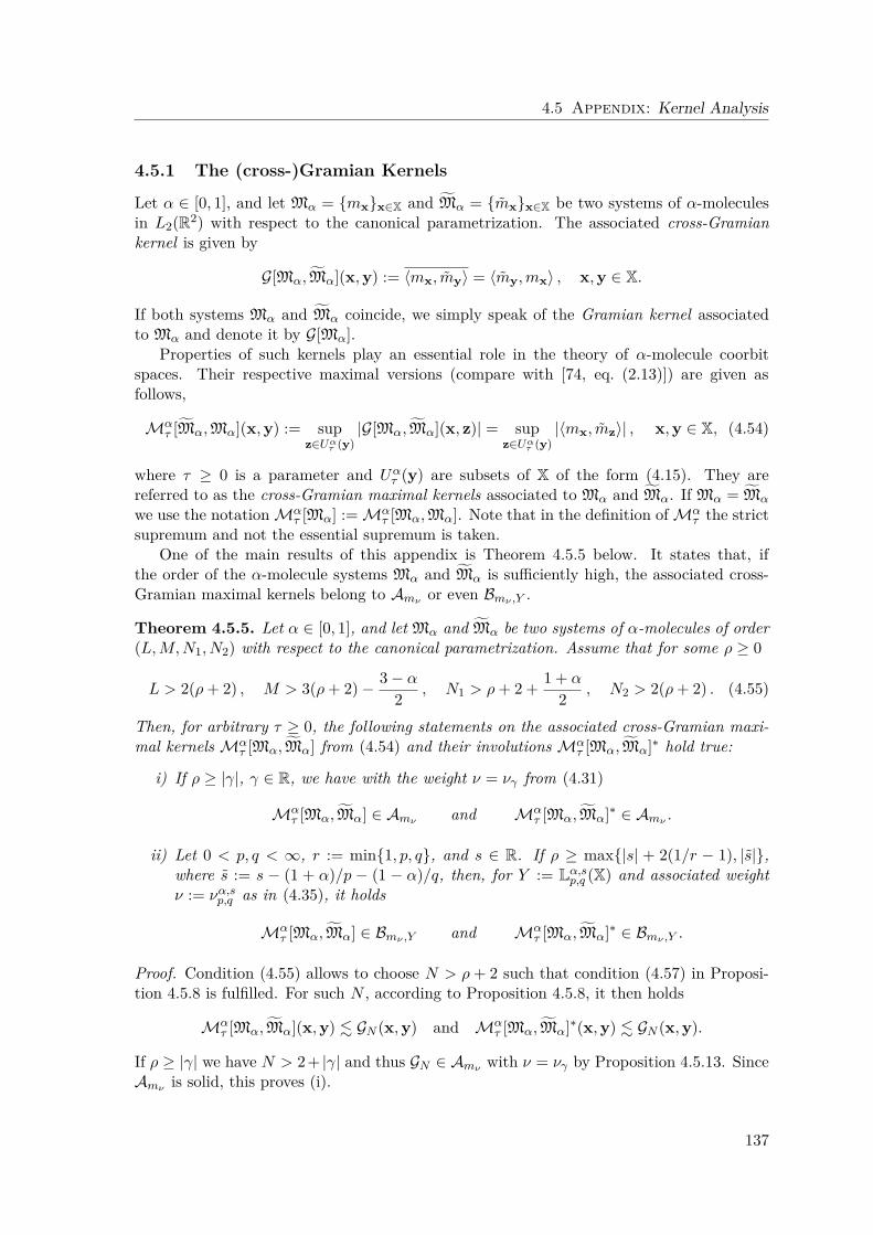
4.5 Appendix: Kernel Analysis
4.5.1 The (cross-)Gramian Kernels
Let α ∈ [0, 1], and let Mα = mxx∈X and Mα = mxx∈X be two systems of α-moleculesin L2(R2) with respect to the canonical parametrization. The associated cross-Gramiankernel is given by
G[Mα,Mα](x,y) := ⟨mx, my⟩ = ⟨my,mx⟩ , x,y ∈ X.
If both systems Mα and Mα coincide, we simply speak of the Gramian kernel associatedto Mα and denote it by G[Mα].
Properties of such kernels play an essential role in the theory of α-molecule coorbitspaces. Their respective maximal versions (compare with [74, eq. (2.13)]) are given asfollows,
Mατ [Mα,Mα](x,y) := sup
z∈Uατ (y)
|G[Mα,Mα](x, z)| = supz∈Uα
τ (y)|⟨mx, mz⟩| , x,y ∈ X, (4.54)
where τ ≥ 0 is a parameter and Uατ (y) are subsets of X of the form (4.15). They are
referred to as the cross-Gramian maximal kernels associated to Mα and Mα. If Mα = Mα
we use the notation Mατ [Mα] := Mα
τ [Mα,Mα]. Note that in the definition of Mατ the strict
supremum and not the essential supremum is taken.One of the main results of this appendix is Theorem 4.5.5 below. It states that, if
the order of the α-molecule systems Mα and Mα is sufficiently high, the associated cross-Gramian maximal kernels belong to Amν or even Bmν ,Y .
Theorem 4.5.5. Let α ∈ [0, 1], and let Mα and Mα be two systems of α-molecules of order(L,M,N1, N2) with respect to the canonical parametrization. Assume that for some ρ ≥ 0
L > 2(ρ+ 2) , M > 3(ρ+ 2) − 3 − α
2 , N1 > ρ+ 2 + 1 + α
2 , N2 > 2(ρ+ 2) . (4.55)
Then, for arbitrary τ ≥ 0, the following statements on the associated cross-Gramian maxi-mal kernels Mα
τ [Mα,Mα] from (4.54) and their involutions Mατ [Mα,Mα]∗ hold true:
i) If ρ ≥ |γ|, γ ∈ R, we have with the weight ν = νγ from (4.31)
Mατ [Mα,Mα] ∈ Amν and Mα
τ [Mα,Mα]∗ ∈ Amν .
ii) Let 0 < p, q < ∞, r := min1, p, q, and s ∈ R. If ρ ≥ max|s| + 2(1/r − 1), |s|,where s := s − (1 + α)/p − (1 − α)/q, then, for Y := Lα,s
p,q (X) and associated weightν := να,s
p,q as in (4.35), it holds
Mατ [Mα,Mα] ∈ Bmν ,Y and Mα
τ [Mα,Mα]∗ ∈ Bmν ,Y .
Proof. Condition (4.55) allows to choose N > ρ+ 2 such that condition (4.57) in Proposi-tion 4.5.8 is fulfilled. For such N , according to Proposition 4.5.8, it then holds
Mατ [Mα,Mα](x,y) . GN (x,y) and Mα
τ [Mα,Mα]∗(x,y) . GN (x,y).
If ρ ≥ |γ| we have N > 2+ |γ| and thus GN ∈ Amν with ν = νγ by Proposition 4.5.13. SinceAmν is solid, this proves (i).
137
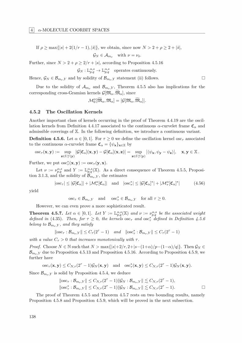
4 α-MOLECULE COORBIT SPACES
If ρ ≥ max|s| + 2(1/r − 1), |s|, we obtain, since now N > 2 + ρ ≥ 2 + |s|,GN ∈ Amν with ν = νs.
Further, since N > 2 + ρ ≥ 2/r + |s|, according to Proposition 4.5.16GN : Lα,s
p,q → Lα,sp,q operates continuously.
Hence, GN ∈ Bmν ,Y and by solidity of Bmν ,Y statement (ii) follows.
Due to the solidity of Amν and Bmν ,Y , Theorem 4.5.5 also has implications for thecorresponding cross-Gramian kernels G[Mα,Mα], since
Mα0 [Mα,Mα] =
G[Mα,Mα].
4.5.2 The Oscillation Kernels
Another important class of kernels occurring in the proof of Theorem 4.4.19 are the oscil-lation kernels from Definition 4.4.17 associated to the continuous α-curvelet frame Cα andadmissible coverings of X. In the following definition, we introduce a continuous variant.Definition 4.5.6. Let α ∈ [0, 1]. For τ ≥ 0 we define the oscillation kernel oscτ associatedto the continuous α-curvelet frame Cα = ψxx∈X by
oscτ (x,y) := supz∈Uα
τ (y)
G[Cα](x,y) − G[Cα](x, z) = sup
z∈Uατ (y)
⟨ψx, ψy − ψz⟩, x,y ∈ X .
Further, we put osc∗τ (x,y) := oscτ (y,x).
Let ν := να,sp,q and Y := Lα,s
p,q (X). As a direct consequence of Theorem 4.5.5, Proposi-tion 3.1.3, and the solidity of Bmν ,Y , the estimates
|oscτ | ≤ |G[Cα]| + |Mατ [Cα]| and |osc∗
τ | ≤ |G[Cα]∗| + |Mατ [Cα]∗| (4.56)
yieldoscτ ∈ Bmν ,Y and osc∗
τ ∈ Bmν ,Y for all τ ≥ 0.However, we can even prove a more sophisticated result.
Theorem 4.5.7. Let α ∈ [0, 1]. Let Y := Lα,sp,q (X) and ν := να,s
p,q be the associated weightdefined in (4.35). Then, for τ ≥ 0, the kernels oscτ and osc∗
τ defined in Definition 4.5.6belong to Bmν ,Y , and they satisfy
∥oscτ : Bmν ,Y ∥ ≤ Cτ (2τ − 1) and ∥osc∗τ : Bmν ,Y ∥ ≤ Cτ (2τ − 1)
with a value Cτ > 0 that increases monotonically with τ .Proof. Choose N ∈ N such that N > max|s|+2/r, 2+|s−(1+α)/p−(1−α)/q|. Then GN ∈Bmν ,Y due to Proposition 4.5.13 and Proposition 4.5.16. According to Proposition 4.5.9, wefurther have
oscτ (x,y) ≤ CN,τ (2τ − 1)GN (x,y) and osc∗τ (x,y) ≤ CN,τ (2τ − 1)GN (x,y).
Since Bmν ,Y is solid by Proposition 4.5.4, we deduce∥oscτ : Bmν ,Y ∥ ≤ CN,τ (2τ − 1)∥GN : Bmν ,Y ∥ . CN,τ (2τ − 1),∥osc∗
τ : Bmν ,Y ∥ ≤ CN,τ (2τ − 1)∥GN : Bmν ,Y ∥ . CN,τ (2τ − 1).The proof of Theorem 4.5.5 and Theorem 4.5.7 rests on two bounding results, namely
Proposition 4.5.8 and Proposition 4.5.9, which will be proved in the next subsection.
138
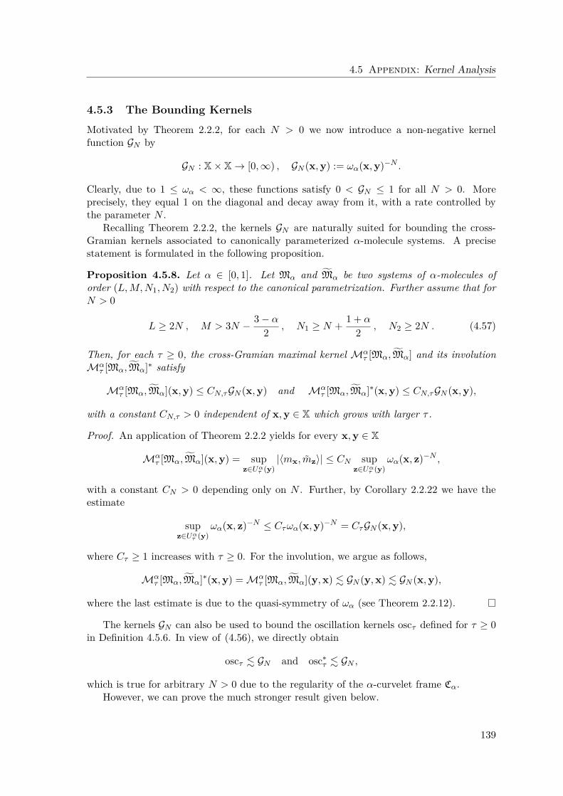
4.5 Appendix: Kernel Analysis
4.5.3 The Bounding Kernels
Motivated by Theorem 2.2.2, for each N > 0 we now introduce a non-negative kernelfunction GN by
GN : X × X → [0,∞) , GN (x,y) := ωα(x,y)−N .
Clearly, due to 1 ≤ ωα < ∞, these functions satisfy 0 < GN ≤ 1 for all N > 0. Moreprecisely, they equal 1 on the diagonal and decay away from it, with a rate controlled bythe parameter N .
Recalling Theorem 2.2.2, the kernels GN are naturally suited for bounding the cross-Gramian kernels associated to canonically parameterized α-molecule systems. A precisestatement is formulated in the following proposition.
Proposition 4.5.8. Let α ∈ [0, 1]. Let Mα and Mα be two systems of α-molecules oforder (L,M,N1, N2) with respect to the canonical parametrization. Further assume that forN > 0
L ≥ 2N , M > 3N − 3 − α
2 , N1 ≥ N + 1 + α
2 , N2 ≥ 2N . (4.57)
Then, for each τ ≥ 0, the cross-Gramian maximal kernel Mατ [Mα,Mα] and its involution
Mατ [Mα,Mα]∗ satisfy
Mατ [Mα,Mα](x,y) ≤ CN,τ GN (x,y) and Mα
τ [Mα,Mα]∗(x,y) ≤ CN,τ GN (x,y),
with a constant CN,τ > 0 independent of x,y ∈ X which grows with larger τ .
Proof. An application of Theorem 2.2.2 yields for every x,y ∈ X
Mατ [Mα,Mα](x,y) = sup
z∈Uατ (y)
|⟨mx, mz⟩| ≤ CN supz∈Uα
τ (y)ωα(x, z)−N ,
with a constant CN > 0 depending only on N . Further, by Corollary 2.2.22 we have theestimate
supz∈Uα
τ (y)ωα(x, z)−N ≤ Cτωα(x,y)−N = Cτ GN (x,y),
where Cτ ≥ 1 increases with τ ≥ 0. For the involution, we argue as follows,
Mατ [Mα,Mα]∗(x,y) = Mα
τ [Mα,Mα](y,x) . GN (y,x) . GN (x,y),
where the last estimate is due to the quasi-symmetry of ωα (see Theorem 2.2.12).
The kernels GN can also be used to bound the oscillation kernels oscτ defined for τ ≥ 0in Definition 4.5.6. In view of (4.56), we directly obtain
oscτ . GN and osc∗τ . GN ,
which is true for arbitrary N > 0 due to the regularity of the α-curvelet frame Cα.However, we can prove the much stronger result given below.
139
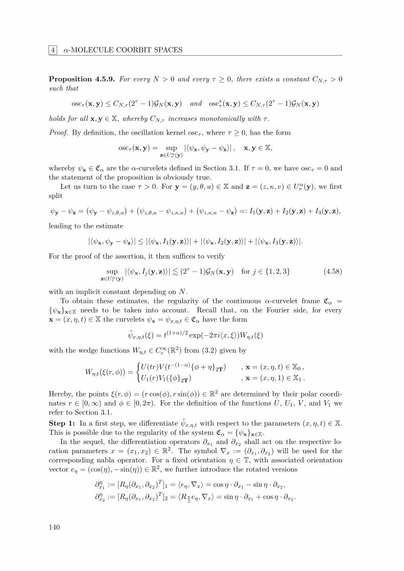
4 α-MOLECULE COORBIT SPACES
Proposition 4.5.9. For every N > 0 and every τ ≥ 0, there exists a constant CN,τ > 0such that
oscτ (x,y) ≤ CN,τ (2τ − 1)GN (x,y) and osc∗τ (x,y) ≤ CN,τ (2τ − 1)GN (x,y)
holds for all x,y ∈ X, whereby CN,τ increases monotonically with τ .
Proof. By definition, the oscillation kernel oscτ , where τ ≥ 0, has the form
oscτ (x,y) = supz∈Uα
τ (y)|⟨ψx, ψy − ψz⟩| , x,y ∈ X,
whereby ψx ∈ Cα are the α-curvelets defined in Section 3.1. If τ = 0, we have oscτ = 0 andthe statement of the proposition is obviously true.
Let us turn to the case τ > 0. For y = (y, θ, u) ∈ X and z = (z, κ, v) ∈ Uατ (y), we first
split
ψy − ψz =ψy − ψz,θ,u
+ψz,θ,u − ψz,κ,u
+ψz,κ,u − ψz
=: I1(y, z) + I2(y, z) + I3(y, z),
leading to the estimate
|⟨ψx, ψy − ψz⟩| ≤ |⟨ψx, I1(y, z)⟩| + |⟨ψx, I2(y, z)⟩| + |⟨ψx, I3(y, z)⟩|.
For the proof of the assertion, it then suffices to verify
supz∈Uα
τ (y)|⟨ψx, Ij(y, z)⟩| . (2τ − 1)GN (x,y) for j ∈ 1, 2, 3 (4.58)
with an implicit constant depending on N .To obtain these estimates, the regularity of the continuous α-curvelet frame Cα =
ψxx∈X needs to be taken into account. Recall that, on the Fourier side, for everyx = (x, η, t) ∈ X the curvelets ψx = ψx,η,t ∈ Cα have the form
ψx,η,t(ξ) = t(1+α)/2 exp(−2πi⟨x, ξ⟩)Wη,t(ξ)
with the wedge functions Wη,t ∈ C∞c (R2) from (3.2) given by
Wη,tξ(r, φ)
=U(tr)V (t−(1−α)φ+ η2T) , x = (x, η, t) ∈ X0 ,
U1(r)V1(φ2T) , x = (x, η, 1) ∈ X1 .
Hereby, the points ξ(r, φ) = (r cos(φ), r sin(φ)) ∈ R2 are determined by their polar coordi-nates r ∈ [0,∞) and φ ∈ [0, 2π). For the definition of the functions U , U1, V , and V1 werefer to Section 3.1.Step 1: In a first step, we differentiate ψx,η,t with respect to the parameters (x, η, t) ∈ X.This is possible due to the regularity of the system Cα = ψxx∈X.
In the sequel, the differentiation operators ∂x1 and ∂x2 shall act on the respective lo-cation parameters x = (x1, x2) ∈ R2. The symbol ∇x := (∂x1 , ∂x2) will be used for thecorresponding nabla operator. For a fixed orientation η ∈ T, with associated orientationvector eη = (cos(η),− sin(η)) ∈ R2, we further introduce the rotated versions
∂ηx1 := [Rη(∂x1 , ∂x2)T ]1 = ⟨eη,∇x⟩ = cos η · ∂x1 − sin η · ∂x2 ,
∂ηx2 := [Rη(∂x1 , ∂x2)T ]2 = ⟨Rπ
2eη,∇x⟩ = sin η · ∂x1 + cos η · ∂x2 .
140
4.5 Appendix: Kernel Analysis
Here, the brackets [·]1 and [·]2 evaluate the first and second component, respectively.At a fixed position x = (x, η, t) ∈ X, we obtain for ξ ∈ R2
∂ηx1ψx,η,t(ξ) = ∂η
x1
t(1+α)/2Wη,t(ξ) exp(−2πi⟨x, ξ⟩)
= −2πi[Rηξ]1t(1+α)/2Wη,t(ξ) exp(−2πi⟨x, ξ⟩)
= t−1t(1+α)/2W[1]η,t(ξ) exp(−2πi⟨x, ξ⟩)
=: t−1 ψ[1]
x,η,t(ξ)
with W[1]η,t(ξ) := −2πit[Rηξ]1Wη,t(ξ).
Similarly, we calculate
∂ηx2ψx,η,t(ξ) = ∂η
x2
t(1+α)/2Wη,t(ξ) exp(−2πi⟨x, ξ⟩)
= −2πi[Rηξ]2t(1+α)/2Wη,t(ξ) exp(−2πi⟨x, ξ⟩)
= t−αt(1+α)/2W[2]η,t(ξ) exp(−2πi⟨x, ξ⟩)
=: t−α ψ[2]
x,η,t(ξ)
with W[2]η,t(ξ) := −2πitα[Rηξ]2Wη,t(ξ).
We proceed with the differentiation ∂η with respect to the parameter η ∈ T. Here weobtain for x = (x, η, t) ∈ X0
∂ηψx,η,t(ξ) = ∂η
t(1+α)/2U(tr)V (t−(1−α)φ+ η2T) exp(−2πi⟨x, ξ⟩)
= t−(1−α)
t(1+α)/2U(tr)V ′(t−(1−α)φ+ η2T) exp(2πi⟨x, ξ⟩)
.
For x = (x, η, 1) ∈ X1 the derivative vanishes,
∂ηψx,η,1(ξ) = ∂η
U1(r)V1(φ2T) exp(−2πi⟨x, ξ⟩)
= 0.
These results motivate the definition
W[η]η,t (ξ(r, φ)) :=
U(tr)V ′(t−(1−α)φ+ η2T) , x = (x, η, t) ∈ X0,
0 , x = (x, η, 1) ∈ X1,
and further
ψ[η]x,η,t(ξ) := t(1+α)/2W
[η]η,t (ξ) exp(2πi⟨x, ξ⟩).
Then we can write
∂ηψx,η,t(ξ) = t−(1−α) ψ[η]
x,η,t(ξ).
For the differentiation operator with respect to the scale variable t ∈ (0, 1) we shallsubsequently use the symbol ∂t. We calculate for x = (x, η, t) ∈ X0
∂tψx,η,t(ξ) = ∂t
t(1+α)/2U(tr)V (t−(1−α)φ+ η2T) exp(2πi⟨x, ξ⟩)
= t−1 ·
t(1+α)/2W
[t]η,t(ξ) exp(2πi⟨x, ξ⟩)
=: t−1 ψ[t]
x,η,t(ξ) ,
141
4 α-MOLECULE COORBIT SPACES
where W [t]η,t(ξ) is the sum
W[t]η,t(ξ) := W
[t,0]η,t (ξ) +W
[t,1]η,t (ξ).+W
[t,2]η,t (ξ).
With U [t] ∈ C∞c ([0,∞)) and V [t] ∈ C∞
c ([−π, π]) given by
U [t](r) := rU ′(r) and V [t](φ) := φV ′(φ),
the summands of this sum are the functions
W[t,0]η,t (ξ(r, φ)) := 1 + α
2 Wη,t(ξ(r, φ)),
W[t,1]η,t (ξ(r, φ)) := U [t](tr)V (t−(1−α)φ+ η2T),
W[t,2]η,t (ξ(r, φ)) := (α− 1)U(tr)V [t](t−(1−α)φ+ η2T).
Finally, for x = (x, η, 1) ∈ X1, we introduce the functions ψ[t]x,η,1 := 0.
By parameter differentiation we have thus derived new function systems from Cα, namely
C[1]α :=
ψ
[1]x
x∈X, C[2]α :=
ψ
[2]x
x∈X, C[η]α :=
ψ
[η]x
x∈X, C[t]α :=
ψ
[t]x
x∈X .
Step 2: Next, we verify that these systems are instances of continuous α-molecules of order(∞,∞,∞,∞) with respect to the canonical parametrization, as Cα = ψxx∈X itself.
The reason for this is that the modified wedge functions W [1]η,t , W
[2]η,t , W
[η]η,t , W [t,0]
η,t , W [t,1]η,t ,
and W[t,2]η,t are all built in the same way as the original functions Wη,t. Indeed, for W [η]
η,t ,W
[t,0]η,t , W [t,1]
η,t , and W[t,2]η,t this is already clear from the above representations. Concerning
W[1]η,t , and W [2]
η,t , in polar representation ξ(r, φ) = (r cos(φ), r sin(φ)), we have with U [1](r) :=rU(r) and V [1](φ) := V (φ)
W[1]η,t(ξ(r, φ)) := −2πi cos(φ+ η2T)U [1](tr)V [1](t−(1−α)φ+ η2T).
Further, with U [2](r) = rU(r) and V [2](φ) = φV (φ), it holds
W[2]η,t(ξ(r, φ)) := −2πisin(φ+ η2T)
φ+ η2TU [2](tr)V [2](t−(1−α)φ+ η2T)
The remaining arguments are then analogous to those used in the proof of Proposi-tion 3.1.3. They are based on the smoothness and support properties of the functions U [1],V [1], U [2], V [2], U [t], V [t], and V ′, which are similar to the properties of U and V .Step 3: In the final step, we provide the desired estimates in (4.58) for j ∈ 1, 2, 3.
Let us first assume y = (y, θ, u) ∈ X0 and z = (z, κ, v) ∈ Uατ (y). In this case, z ∈ X0
and it holds (see definition of Uατ (y) in (4.15))
z := z − y ∈ R−1θ Aα,uQ
τ , κ := κ− θ2T ∈ u1−αIτ , v := v/u ∈ Jτ .
Using the fundamental theorem of calculus, we obtain for ξ ∈ R2
I1(ξ) = ψy,θ,u(ξ) − ψy+z,θ,u(ξ) = − 1
0⟨∇yψy+(1−a)z,θ,u(ξ), z⟩ da
= −u−1 1
0ψ
[1]y+az,θ,u(ξ)[Rθz]1 da− u−α
1
0ψ
[2]y+az,θ,u(ξ)[Rθz]2 da.
142
4.5 Appendix: Kernel Analysis
Similarly, with κ = κ− θ2T, we get for fixed ξ ∈ R2
I2(ξ) = ψz,θ,u(ξ) − ψz,(θ+κ)2π ,u(ξ) = 0
κ∂ηψz,(θ+a)2π ,u(ξ) da = u−(1−α)
0
κψ
[η]z,(θ+a)2π ,u(ξ) da.
Hereby (θ + a)2π is the value of θ + a modulo 2π. Further, it holds for v = v/u and ξ ∈ R2
I3(ξ) = ψz,κ,u(ξ) − ψz,κ,vu(ξ) = u
vu∂tψz,κ,a(ξ) da = u−1
u
vuψ[t]
z,κ,a(ξ) da = 1
vψ[t]
z,κ,au(ξ) da.
Using the Plancherel theorem and the theorem of Fubini-Tonelli, we deduce for arbitraryx ∈ X, y ∈ X0, and z ∈ Uα
τ (y)
⟨ψx, I1(y, z)⟩ =
[Rθz]1u
ψx,
10
ψ[1]y+az,θ,u da
+ [Rθz]2
uα
ψx,
10
ψ[2]y+az,θ,u da
≤ |[Rθz]1|
u
10
⟨ψx, ψ[1]y+az,θ,u⟩
da+ |[Rθz]2|uα
10
⟨ψx, ψ[2]y+az,θ,u⟩
da≤ |[Rθz]1|
uMα
τ [C[1]α ,Cα](x,y) + |[Rθz]2|
uαMα
τ [C[2]α ,Cα](x,y) .
From z ∈ R−1θ Aα,uQ
τ we deduce Rθz ∈ Aα,uQτ and hence |[Rθz]1| ≤ τu and |[Rθz]2| ≤
τuα. Invoking Proposition 4.5.8, we arrive at the estimate⟨ψx, I1(y, z)⟩ ≤ CN,ττGN (x,y) ,
from which the desired estimate for j = 1 in (4.58) follows due to τ ≤ 2τ − 1.Similarly, we estimate the two other terms corresponding to j ∈ 2, 3 in (4.58). Since
κ ∈ u1−αIτ , we have |κ| ≤ τu1−α and thus⟨ψx, I2(y, z)⟩ =
⟨ψx, I2(y, z)⟩ = u−(1−α)
ψx,
κ
0ψ
[η]z,(θ+a)2π ,u(ξ) da
≤ u−(1−α)
|κ|
0
⟨ψx, ψ[η]z,(θ+a)2π ,u⟩
da ≤ u−(1−α) |κ|
0Mα
τ [C[η]α ,Cα](x,y) da
≤ CN,τu−(1−α)|κ|GN (x,y) ≤ CN,ττGN (x,y).
Finally, due to v ∈ Jτ = [2−τ , 2τ ] we have |1 − v| ≤ 2τ − 1. This yields⟨ψx, I3(y, z)⟩ =
⟨ψx, I3(y, z)⟩ =
ψx,
1
vψ[t]
z,κ,au(ξ) da
≤ 1
v
⟨ψx, ψ[t]z,κ,au⟩
da ≤ 1
v
Mατ [C[t]
α ,Cα](x,y) da
≤ CN,τ |1 − v|GN (x,y) ≤ CN,τ (2τ − 1)GN (x,y).
It remains to handle the case y ∈ X1. Here the estimates are trivial for j ∈ 2, 3 sinceI2(y, z) = I3(y, z) = 0. For j = 1 the arguments are the same as before.
Concerning the estimate of the involuted kernel osc∗τ , we can argue with the quasi-
symmetry of GN which directly follows from the quasi-symmetry of ωα (see Theorem 2.2.12).
143
4 α-MOLECULE COORBIT SPACES
In the following, we will deduce sufficient conditions for GN to belong to Amν andBmν ,Y . Together with solidity arguments based on Propositions 4.5.8 and 4.5.9, those arethe foundation for the proof of Theorem 4.5.5 and Theorem 4.5.7.
4.5.4 The Convolution-Type Auxiliary Kernels
For the subsequent investigation, it is useful to introduce another scale of kernels with aconvolution-type structure. For N > 0, let us introduce
HN : X × X → [0,∞) , HN (x,y) := max tu,u
t
−N1 + d′
α(x,y)−N
,
where, with e1 and e2 denoting the respective unit vectors of R2,
d′α(x,y) := |η − θ|2
maxt, u2(1−α) +|⟨R−1
η e2, x− y⟩|2
maxt, u2α+
|⟨R−1η e1, x− y⟩|maxt, u
.
Hereby, the bracket · = ·T denotes the projective bracket defined in (2.9). For conve-nience, we will often use the short-hand notation (t, u)+ := maxt, u for t, u ∈ R in thesequel.
The kernels HN can also be written in the form
HN (x,y) = HN
A−1
α,tRη(y − x), t−(1−α)θ − η, u/t
with non-negative functions HN : R2 × R × R+ → [0,∞) given by
HN (a, b, c) := maxc, c−1−N
1 + |b|2
max1, c2(1−α) + |[a]2|2
max1, c2α+ |[a]1|
max1, c
−N
.
(4.59)
Clearly, from the definition, 0 < HN (a, b, c) ≤ 1 for all (a, b, c) ∈ R2 × R × R+.An important relation of HN to the kernels GN and G∗
N are the following estimates.
Lemma 4.5.10. For every N > 0 we have
GN (x,y) . HN (x,y) and G∗N (x,y) . HN (x,y) , x,y ∈ X.
Proof. Recall the simplified index distance ωsimα from Definition 2.2.3 given by
ωsimα (x,y) = max
tu,u
t
1 + dsim
α (x,y)
withdsim
α (x,y) = |η − θ|2
maxt, u2(1−α) + |x− y|2
maxt, u2α+
|⟨R−1η e1, x− y⟩|maxt, u
.
It was proved in Lemma 2.2.4 that ωα(x,y) & ωsimα (x,y) and dα(x,y) & dsim
α (x,y). Since|⟨R−1
η e2, x− y⟩| ≤ |x− y| we can deduce
dα(x,y) & dsimα (x,y) ≥ d′
α(x,y).
The assertion follows.
144
4.5 Appendix: Kernel Analysis
As a consequence of these estimates, a sufficient condition for HN to belong to Amν
and Bmν ,Y allows to deduce such conditions for GN and G∗N . The advantage of the kernels
HN is their convolution-type structure. Due to this structure, the analysis of HN can bereduced to an analysis of the corresponding function HN given by (4.59), which is a greatsimplification.
One could pose the question, why the kernels GN are defined after all, if we could directlyuse HN as bounding kernels. The reason for this is that the kernels HN do not possess thesame symmetry and stability properties as GN (see Corollary 2.2.9 and Corollary 2.2.22).
In the sequel, the integrability properties of HN stated in the next lemma are essential.
Lemma 4.5.11. Let 0 < r ≤ 1, γ ∈ R, and N > 2/r + maxγ, 0. ThenR+
R
R2
HN (y, θ, u)r maxu, u−1rγ(u+ 1)2dy dθ du
u3 < ∞ ,
R
R2
HN (y, θ, 1)r dy dθ < ∞ .
Proof. For fixed u ∈ R+, let us first consider the inner integral
I(u) :=R
R2
HN (y, θ, u)r dy dθ.
Generally, we have for quantities R > 0, c > 0, γ > 0, and N > 1γ the formula
∞0
(R+ c−γaγ)−N da ≍∞
0
(R1/γ + c−1a)−γN da = c ·∞
R1/γ
a−γN da
= c
1 − γN
a−γN+1
∞R1/γ
= c
γN − 1R−(N−1/γ) ≍ c ·R−(N−1/γ) .
Applying this formula iteratively, we can calculate I(u). For N > 2/r and u ∈ R+ weobtain
I(u) = maxu, u−1−NrR
R2
1 + |θ|2
max1, u2(1−α) + |[y]2|2
max1, u2α+ |[y]1|
max1, u
−Nrdy dθ
≍ maxu, u−1−Nr max1, u2.
Specifically for u = 1, this implies I(1) ≍ 1 < ∞ proving the second assertion.To obtain the first assertion, we evaluate the outer integral over the scales, namelyR+I(u) maxu, u−1rγ(u+ 1)2du
u3 ≍ ∞
0maxu, u−1−Nr+γr max1, u2(u+ 1)2 du
u3
= 1
0uNr−γr−2(u+ 1)2 du
u+ ∞
1u−Nr+γr+2 (u+ 1)2
u2du
u
≍ 1
0uNr−γr−2 du
u+ ∞
1u−(Nr−γr−2) du
u< ∞ .
Precisely if Nr − γr − 2 > 0, or equivalently N > 2/r + γ, the last two integrals converge.Since the assumption N > 2/r + maxγ, 0 ensures both N > 2/r as well as N > 2/r + γ,the proof is finished.
145
4 α-MOLECULE COORBIT SPACES
Another important auxiliary result concerning HN is the following lemma.
Lemma 4.5.12. It holds, uniformly in (x, η, t) ∈ R2 × R × R+,
inf(κ,v)∈I×J
HN (x, η + t1−ακ, tv) ≍ HN (x, η, t) ≍ sup(κ,v)∈I×J
HN (x, η + t1−ακ, tv),
where I := [−1, 1] and J := [ 12 , 2].
Proof. Let us define HN (x, η, t) := sup(κ,v)∈I×J HN (x, η + t1−ακ, tv) and H ′N (x, η, t) :=
inf(κ,v)∈I×J HN (x, η + t1−ακ, tv). Clearly, H ′N (x, η, t) ≤ HN (x, η, t) ≤ HN (x, η, t). For the
opposite estimates, we first note that for c ∈ R+
infv∈cJ
maxv, v−1 ≍ supv∈cJ
maxv, v−1 and infv∈cJ
max1, v ≍ supv∈cJ
max1, v.
Further, the estimate |η + t1−ακ|2 ≤ 2|η|2 + 2 max1, t2(1−α)|κ|2 yields
supκ∈I
|η + t1−ακ|2
max1, t2(1−α) ≤ 2|η|2
max1, t2(1−α) + 2.
Similarly, |η|2 ≤ 2|η − t1−ακ|2 + 2 max1, t2(1−α)|κ|2 leads to
infκ∈I
|η + t1−ακ|2
max1, t2(1−α) ≥ |η|2
2 max1, t2(1−α) − 1.
Altogether, all these ingredients yield HN (x, η, t) . HN (x, η, t) . H ′N (x, η, t).
After this preparation, we are now ready to prove conditions on N ensuring the mem-bership of HN , and in turn GN and G∗
N , in the algebras Amν and Bmν ,Y .
4.5.5 Kernel Criteria for GN ∈ Amν and GN ∈ Bmν ,Y
In this last subsection of the appendix we aim for an easily applicable criterion to be ableto decide whether a kernel GN belongs to the algebra Bmν ,Y , where either Y := Ls
p,q(X) orY := Lα,s
p,q (X) and ν is the respective associated weight.As a first step, we prove a simple criterion which ensures that GN belongs to the algebra
Amν with a weight ν = νγ of the form (4.31) with γ ∈ R. The following proposition showsthat there exists a threshold for N above which GN ∈ Amν is guaranteed. This is notsurprising since a large N promotes a fast off-diagonal decay of GN .
Proposition 4.5.13. Let γ ∈ R and let ν = νγ be the weight defined in (4.31). If N > 2+|γ|then GN is an element of Amν .
Proof. According to Lemma 4.5.10 we have
GN (x,y) . HN (x,y) = HN
A−1
α,tRη(y − x), t−(1−α)θ − η, u/t,
where HN is the function from (4.59). An application of Lemma 4.5.15, which is provedbelow, then yields the assertion. We only need to verify that the quantities Ai, i ∈ 1, 2, 3,associated to HN are finite if N > 2 + |γ|.
146
4.5 Appendix: Kernel Analysis
For the quantities A1 and A3 this follows directly from Lemma 4.5.11 which asserts
A1 =R+
R
R2
HN (y, θ, u) maxu, u−1|γ|(u+ 1)2dy dθ du
u3 < ∞ ,
A3 =T
R2
HN (y, θ, 1) dy dθ ≤R
R2
HN (y, θ, 1) dy dθ < ∞ .
Using Lemma 4.5.14 and Lemma 4.5.12, we can further show that A2 . A1. Indeed, notingthat dt/t is the Haar measure of the multiplicative group R+, we have with the windowJ := [ 1
2 , 2] ⊂ R+
A2 ≤ ess supu∈R+
ess sup
v∈uJ
R
R2
|HN (y, θ, v)| maxv, v−1|γ|(1 + v)−2 dy dθ
.R+
R
R2
ess supv∈uJ
|HN (y, θ, v)| maxv, v−1|γ| dy dθduu
.R+
R
R2
|HN (y, θ, u)| maxu, u−1|γ| dy dθ du
u≤ A1.
As a consequence, also A2 < ∞ holds true if N > 2 + |γ|.
In the proof of the previous proposition, we have implicitly used an embedding resultfor Wiener amalgam spaces. It can be termed as an estimate of the corresponding quasi-norms. Given an arbitrary measure space (X, µ) and 0 < p ≤ ∞, let Lp(X) denote the usualLebesgue space on X with quasi-norm ∥ · |Lp∥. Further, assume that Wxx∈X is a familyof measurable windows Wx ⊆ X such that the associated dual windows Wx ⊆ X defined bythe relation X Wx
(y) = XWy(x) are also measurable. Then we have the following estimate.
Lemma 4.5.14. If there is m > 0 such that µ(Wx) ≥ m holds independently of x ∈ X,then we have for 0 < p ≤ q ≤ ∞ and every measurable function f : X → C the estimate
∥Kf |Lq∥ ≤ m1/q−1/p∥Kf |Lp∥,
where Kf(x) := ess supy∈X |f(y)|XWx(y) is a Wiener control function as in (4.14).Proof. We restrict the proof to the case q < ∞, with obvious modifications if q = ∞.
First, we observe that ∥Kf |L∞∥ = ∥f |L∞∥. Second, we see that
∥Kf |Lq∥q =X
ess supy∈X
|f(y)XWx(y)|q dµ(x)
≥ ess supy∈X
X
|f(y)|qXWx(y) dµ(x) ≥ m∥Kf |L∞∥q.
Since |Kf |/∥Kf |L∞∥ ≤ 1 almost everywhere, we can deduce for p ≤ q
m ≤ ∥Kf |Lq∥q
∥Kf |L∞∥q≤ ∥Kf |Lp∥p
∥Kf |L∞∥p.
Since 1/q ≤ 1/p, this further implies∥Kf |Lq∥
∥Kf |L∞∥m1/q≤ ∥Kf |Lp∥
∥Kf |L∞∥m1/p,
and therefore ∥Kf |Lq∥ ≤ m1/q−1/p∥Kf |Lp∥.
147
4 α-MOLECULE COORBIT SPACES
Note that the proven estimate ∥Kf |Lq∥ . ∥Kf |Lp∥ for 0 < p ≤ q ≤ ∞ resembles therelation ∥ · ∥ℓq ≤ ∥ · ∥ℓp of the discrete Lebesgue quasi-norms. Hence, we can record that theembedding properties of the Wiener amalgams are analogous to those of the correspondingsequence spaces.
Another essential ingredient in the proof of Proposition 4.5.13 is the following technicallemma.
Lemma 4.5.15. Let α ∈ [0, 1], and assume that K : X × X → C is a kernel function andH : R2 × R × R+ → [0,∞) a measurable function such that
|Kx,y
| ≤ H
A−1
α,tRη(y − x), t−(1−α)θ − η, u/t.
Further let γ ∈ R be fixed and let us put T := [−π/2, π/2) and (u, 1)+ := maxu, 1. Thenthe finiteness of the quantities
A1 :=R+
R
R2H(y, θ, u) maxu, u−1|γ|(1 + u)2dy dθ du
u3 ,
A2 := ess supu∈R+
(u,1)1−α
+ T
R2H(y, θ, u) maxu, u−1|γ|(1 + u)−2 dy dθ,
A3 :=
T
R2H(y, θ, 1) dy dθ,
impliesK ∈ Amν with ∥K|Amν ∥ ≤ 2
A1 + max4A2, A3
,
with mν denoting the bivariate weight associated to the weight ν = νγ defined in (4.31).
Proof. For fixed x = (x, η, t) ∈ X we haveX
|K(x,y)|mν(x,y) dµ(y) ≤ 2I0(x) + I1(x)
with the integrals
I0(x) := 12
10
T
R2
HA−1
α,tRη(y − x), t−(1−α)θ − η, u/t(t/u, u/t)|γ|
+dy dθ du
u3 ,
I1(x) := 12
T
R2
HA−1
α,tRη(y − x), t−(1−α)θ − η, 1/tt−|γ| dy dθ.
Eliminating the brackets · in these integrals, they simplify to
I0(x) =1
0
T
R2
HA−1
α,tRη(y − x), t−(1−α)θ, u/t(t/u, u/t)|γ|
+dy dθ du
u3 ,
I1(x) =T
R2
HA−1
α,tRη(y − x), t−(1−α)θ, 1/tt−|γ| dy dθ.
148
4.5 Appendix: Kernel Analysis
Substituting y →→ R−1η Aα,ty + x and θ →→ t1−αθ, we obtain
I0(x) = t21
0
t−(1−α)T
R2
Hy, θ, u/t
(t/u, u/t)|γ|
+dy dθ du
u3 ,
I1(x) = t2
t−(1−α)T
R2
Hy, θ, 1/t
t−|γ| dy dθ .
The substitution u →→ tu further yields
I0(x) =1/t0
t−(1−α)T
R2
Hy, θ, u
(u, 1/u)|γ|
+dy dθ du
u3 .
Now we observe
ess supx∈X
I1(x) = max
ess supx∈X0
I1(x), ess supx∈X1
I1(x)
with the terms
ess supx∈X1
I1(x) =T
R2
Hy, θ, 1
dy dθ = A3,
ess supx∈X0
I1(x) = ess supt>1
t|γ|
t1−αT
R2
Hy, θ, t
dy dθt2
≤ 4A2 .
Further, we have
ess supx∈X
I0(x) = max
ess supx∈X0
I0(x), ess supx∈X1
I0(x)
≤∞
0
R
R2
Hy, θ, u
(u, 1/u)|γ|
+dy dθ du
u3 ≤ A1 .
Analogously, for fixed y = (y, θ, u) ∈ X we getX
|K(x,y)|mν(x,y) dµ(x) ≤ 2I0(y) + I1(y)
with the integrals
I0(y) := 12
10
T
R2
HA−1
α,tRη(y − x), t−(1−α)θ − η, u/t(t/u, u/t)|γ|
+dx dη dt
t3,
I1(y) := 12
T
R2
HRη(y − x), θ − η, u
u−|γ| dx dη.
149
4 α-MOLECULE COORBIT SPACES
We now first use the substitution η →→ θ − η. Then, as before, we eliminate the brackets,
I0(y) = 12
10
T
R2
HA−1
α,tRθ−η(y − x), t−(1−α)η, u/t(t/u, u/t)|γ|
+dx dη dt
t3
=1
0
T
R2
HA−1
α,tRθ−η(y − x), t−(1−α)η, u/t(t/u, u/t)|γ|
+dx dη dt
t3,
I1(y) = 12
T
R2
HRθ−η(y − x), η, u
u−|γ| dx dη
=T
R2
HRθ−η(y − x), η, u
u−|γ| dx dη.
The substitutions x →→ y −R−1θ−ηAα,tx and η →→ t1−αη yield
I0(y) =1
0
t−(1−α)T
R2
Hx, η, u/t
(t/u, u/t)|γ|
+dx dη dt
t,
I1(y) =T
R2
Hx, η, u
u−|γ| dx dη .
Finally, the substitution t →→ u/t gives
I0(y) =∞
u
(t/u)1−αT
R2
Hx, η, t
(t, 1/t)|γ|
+dx dη dt
t.
We obtain
ess supy∈X
I1(y) = max
ess supy∈X0
I1(y), ess supy∈X1
I1(y)
with
ess supy∈X1
I1(y) =T
R2
Hx, η, 1
dx dη = A3,
ess supy∈X0
I1(y) = ess sup0<u<1
T
R2
Hx, η, u
u−|γ| dx dη ≤ 4A2 .
For ess supy∈X
I0(y) = max
ess supy∈X0
I0(y), ess supy∈X1
I0(y)
we get
ess supy∈X
I0(y) ≤R+
R
R2
Hx, η, t
(t, 1/t)|γ|
+dx dη dt
t≤ A1 .
This finishes the proof.
150
4.5 Appendix: Kernel Analysis
We next formulate a sufficient criterion ensuring that the kernel GN operates contin-uously on the function spaces Ls
p,q(X) and Lα,sp,q (X). As in Proposition 4.5.13, it can be
expected that a sufficiently large N provides such a guarantee, since, intuitively, the largerN the closer GN is to the identity operator.
Proposition 4.5.16. Let α ∈ [0, 1], 0 < p, q < ∞, r = min1, p, q, and s ∈ R. IfN > 2
r + |s| then GN operates continuously on Lα,sp,q (X). In the Banach case, i.e., when
r = 1, the kernel GN also operates continuously on Lsp,q(X).
Proof. For every N > 0 and all x,y ∈ X we have by Corollary 2.2.22 and Lemma 4.5.10
sup(a,b)∈Uα
1 (x)×Uα1 (y)
GN (a,b) . GN (x,y) . HN (x,y),
and HN (x,y) = HN ((x, η, t), (y, θ, u)) has the representation
HN (x,y) = HN
A−1
α,tRη(y − x), t−(1−α)θ − η, u/t
with the function HN from (4.59). Hence GN is of the required form to apply Lemma 4.5.17or Lemma 4.5.18.
It only remains to show that the quantities Bi, or Bi respectively, are finite for eachi ∈ 1, . . . , 4. This task is simplified by the following observation. If q ≥ 1 we have ℓ1 → ℓq
and thus – as a consequence of Lemma 4.5.14 and Lemma 4.5.12 – using J := [ 12 , 2] as a
window
B2 ≤ ∞
1
ess sup
v∈uJ
v1−αT
R2
vsHN
y, θ, v
dy dθv2
q du
u
1/q
.R+
R
R2
ess supv∈uJ
vsHN
y, θ, v
dy dθv2
du
u. B1.
Similarly, one can prove B3 . B1, and analogously also B2 . B1 and B3 . B1.Finally, since N > 2/r + |s|, according to Lemma 4.5.11, we have
B1, B1 ≤R+
R
R2
HN (y, θ, u)r maxu, u−1|s|r(u+ 1)2dy dθ du
u3 < ∞ ,
B4, B4 ≤R
R2
HN (y, θ, 1)r dy dθ < ∞ .
As a consequence, all quantities B1, B4, B1, B4 are finite if N > 2/r+ |s|, and the statementis proven.
The proof of the previous proposition builds upon the following two lemmas.
Lemma 4.5.17. Let α ∈ [0, 1], 1 ≤ p, q < ∞, and s ∈ R be fixed. Further, put T :=[−π/2, π/2) and assume that K : X × X → C is a kernel with the property
|Kx,y
| ≤ H
A−1
α,tRη(y − x), t−(1−α)θ − η, u/t
151
4 α-MOLECULE COORBIT SPACES
for some measurable function H : R2 ×R×R+ → [0,∞). Then K is a well-defined boundedoperator
K : Lsp,q(X) → Ls
p,q(X) with ∥K|Lsp,q → Ls
p,q∥ . B1 +B2 +B3 +B4,
provided that, with q′ := q/(q − 1) denoting the dual exponent of q,
B1 :=∞
0
R
R2
usHy, θ, u
dy dθ duu3 < ∞ ,
B2 := ∞
1
u1−αT
R2
usHy, θ, u
dy dθu2
q du
u
1/q
< ∞,
B3 := 1
0
T
R2
usHy, θ, u
dy dθu2
q′du
u
1/q′
< ∞ ,
B4 :=T
R2
Hy, θ, 1
dy dθ < ∞ .
Proof. Due to Lemma 4.5.3 and the solidity of Lsp,q, we can without loss of generality assume
that the kernel K is non-negative. In this special case, for any measurable non-negativefunction F : X → [0,∞), the integral
KF (x) :=X
K(x,y)F (y) dµ(y) , x ∈ X,
has a well-defined value in the extended range [0,∞] at almost all points x ∈ X. One thusobtains a measurable function KF on X with the target set [0,∞]. The investigation belowwill further show that the additional assumption F ∈ Ls
p,q ensures KF ∈ Lsp,q with the
estimate ∥KF |Lsp,q∥ . (B1 +B2 +B3 +B4)∥F |Ls
p,q∥.For an arbitrary, not necessarily non-negative, function F ∈ Ls
p,q we can then argue asfollows. Since |F | ∈ Ls
p,q is non-negative, by the above, we have K|F | ∈ Lsp,q, which in
particular entails K|F |(x) < ∞ for almost all x ∈ X. At those points, KF (x) is containedin C, giving rise to a measurable function KF : X → C. Further, since |KF | ≤ K|F | almosteverywhere, KF ∈ Ls
p,q holds true by solidity and
∥KF |Lsp,q∥ ≤ ∥K|F ||Ls
p,q∥ ≤ (B1 +B2 +B3 +B4)∥|F ||Lsp,q∥ = (B1 +B2 +B3 +B4)∥F |Ls
p,q∥.
This proves the assertion of the lemma. All, that remains to be shown, is that KF ∈ Lsp,q
with ∥KF |Lsp,q∥ ≤ (B1 +B2 +B3 +B4)∥F |Ls
p,q∥ holds true for every non-negative functionF ∈ Ls
p,q. The proof of this claim is split into several steps.Step 1: First we estimate the functions K[FXX0 ]. Thereby we transfer the integrationdomain from P to P via the canonical projection p : P → P defined in (2.12). For this, it isuseful to associate to F : P → [0,∞) the auxiliary function F : P → [0,∞) by
F (y, θ, u) := F (y, θ, u) + F (y, θ + π, u) , θ ∈ [0, π),
where · = ·T denotes the projective bracket from (2.9).
152
4.5 Appendix: Kernel Analysis
Let now x = (x, η, t) ∈ X be fixed. We then have
K[FXX0 ](x) =X0
K(x, η, t), (y, θ, u)
F (y, θ, u) dµ0(y, θ, u)
≤X0
HA−1
α,tRη(y − x), t−(1−α)θ − η, u/tF (y, θ, u) dµ0(y, θ, u)
=1
0
T
R2
HA−1
α,tRη(y − x), t−(1−α)θ − η, u/tF (y, θ, u) dy dθ du
u3 .
Note a + b + c = a + b + c. With the substitutions y →→ R−1η Aα,ty + x, θ →→
t1−αθ + η, u →→ tu, we hence arrive at
K[FXX0 ](x) ≤1/t0
t−(1−α)T
R2
Hy, θ, u
F (R−1
η Aα,ty + x, t1−αθ + η, tu) dy dθ duu3 .
Analogously, one shows with the substitutions y →→ R−1η y + x, θ →→ θ + η,
K[FXX1 ](x) =X1
K(x, η, t), (y, θ, 1)
F (y, θ, 1) dµ1(y, θ, 1)
≤X1
HA−1
α,tRη(y − x), t−(1−α)θ − η, 1/tF (y, θ, 1) dµ1(y, θ, 1)
=T
R2
HA−1
α,tRη(y − x), t−(1−α)θ − η, 1/tF (y, θ, 1) dy dθ
=T
R2
HA−1
α,ty, t−(1−α)θ, 1/t
F (R−1
η y + x, θ + η, 1) dy dθ.
Step 2: For each fixed t ∈ (0, 1], we now decomposeT
∥KF (·, η, t)|Lp∥q dη
1/q
≍
T
∥K[FXX0 ](·, η, t)|Lp∥q dη
1/q
+
T
∥K[FXX1 ](·, η, t)|Lp∥q dη
1/q
=: T0(t) + T1(t).
Then we estimate T0(t) and T1(t), using Step 1 and the continuous Minkowski inequality,
T0(t) ≤
T
1/t0
t−(1−α)T
R2
Hy, θ, u
F (R−1
η Aα,ty + ·, t1−αθ + η, tu) dy dθ duu3
Lp
qdη
1/q
≤1/t0
t−(1−α)T
R2
Hy, θ, u
T
F (R−1η Aα,ty + ·, t1−αθ + η, tu)
Lp
qdη
1/q dy dθ du
u3
=1/t0
t−(1−α)T
R2
Hy, θ, u
T
F (·, η, tu)|Lp
qdη
1/q dy dθ du
u3 ,
153
4 α-MOLECULE COORBIT SPACES
and analogously
T1(t) ≤
T
T
R2
HA−1
α,ty, t−(1−α)θ, 1/t
F (R−1
η y + ·, θ + η, 1) dy dθLp
qdη
1/q
≤T
R2
HA−1
α,ty, t−(1−α)θ, 1/t
T
F (R−1η y + ·, θ + η, 1)
Lp
qdη
1/q
dy dθ
=T
R2
HA−1
α,ty, t−(1−α)θ, 1/t
dy dθ
T
∥F (·, η, 1)|Lp∥q dη
1/q
.
Step 3: Finally, we decompose the kernel K =1
i=01
j=0Ki,j with
Ki,j(x,y) := K(x,y)XXi×Xj (x,y) for (i, j) ∈ 0, 12.
To finish the proof, it then suffices to check that for every (i, j) ∈ 0, 12
Si,j := ∥Ki,jF |Lsp,q∥ . ∥FXXj |Ls
p,q∥.
We start with S0,1 and S1,1 and observe
S1,1 = T1(1) and S0,1 = 1
0
t−sqT1(t)q dt
t
1/q
.
Plugging in the estimates from Step 2, we get
S1,1 ≤T
R2
Hy, θ, 1
dy dθ
T
∥F (·, η, 1)|Lp∥q dη
1/q
.
Further, taking into account
∥FXX1 |Lsp,q∥ ≍
T
∥F (·, η, 1)|Lp∥q dη
1/q
, (4.60)
a relation proved in Step 4 below, this yields
S1,1 . B4 · ∥FXX1 |Lsp,q∥ with B4 =
T
R2
Hy, θ, 1
dy dθ.
For S0,1 we derive from Step 2
S0,1 ≤ 1
0
t−sq
T
R2
HA−1
α,ty, t−(1−α)θ, 1/t
dy dθ
T
∥F (·, η, 1)|Lp∥q dη
1/qq dt
t
1/q
.
We deduce, again with (4.60),
S0,1 . B2 · ∥FXX1 |Lsp,q∥
154
4.5 Appendix: Kernel Analysis
with
B2 = 1
0
t−sq
T
R2
HA−1
α,ty, t−(1−α)θ, 1/t
dy dθ
q dt
t
1/q
= ∞
1
t1−αT
R2
tsHy, θ, t
dy dθt2
q dt
t
1/q
.
Next, we turn to S1,0 and S0,0 given by
S1,0 = T0(1) and S0,0 = 1
0
t−sqT0(t)q dt
t
1/q
.
To estimate S1,0, we use the results of Step 2 and Hölder’s inequality, where q′ shalldenote the dual exponent of q satisfying 1/q + 1/q′ = 1. We obtain
S1,0 ≤1
0
T
R2
Hy, θ, u
T
F (·, η, u)|Lp
qdη1/q dy dθ du
u3
=1
0
T
R2
Hy, θ, u
dy dθu2
·
T
F (·, η, u)|Lp
qdη1/q du
u
≤ 1
0
uq′s
T
R2
Hy, θ, u
dy dθu2
q′ du
u
1/q′
· 1
0u−sq
T
F (·, η, u)|Lp
q dη du
u
1/q.
Using the relation
∥FXX0 |Lsp,q∥ ≍
10
T
t−sq∥F (·, η, t)|Lp∥q dη dt
t
1/q
, (4.61)
whose proof is outsourced to Step 4, we arrive at
S1,0 . B3 · ∥FXX0 |Lsp,q∥ with B3 =
10
T
R2
usH(y, θ, u)dy dθu2
q′ du
u
1/q′
.
Last but not least, we estimate S0,0. Note that X(0,1/t)(u) = X(0,1/u)(t) for t, u ∈ R+.
155
4 α-MOLECULE COORBIT SPACES
S0,0 ≤ 1
0
t−sq 1/t
0
t−(1−α)T
R2
Hy, θ, u
T
F (·, η, tu)|Lp
qdη1/q dy dθ du
u3
q dt
t
1/q
≤ 1
0
t−sq ∞
0
R
R2
X(0,1/t)(u)Hy, θ, u
T
F (·, η, tu)|Lp
qdη1/q dy dθ du
u3
q dt
t
1/q
≤∞
0
R
R2
Hy, θ, u
10
T
t−sqX(0,1/u)(t)F (·, η, tu)|Lp
qdηdt
t
1/q dy dθ du
u3
=∞
0
R
R2
Hy, θ, u
1/u0
T
t−sqF (·, η, tu)|Lp
q dη dt
t
1/q dy dθ du
u3
=∞
0
R
R2
Hy, θ, u
us 1
0
T
t−sqF (·, η, t)|Lp
q dη dt
t
1/q dy dθ du
u3 .
With (4.61), this leads to
S0,0 . B1 · ∥FXX0 |Lsp,q∥ with B1 =
∞0
R
R2
usHy, θ, u
dy dθ duu3 .
Step 4: It remains to show (4.60) and (4.61). First, observe that due to the non-negativityof F for every η ∈ [0, π) and t ∈ (0, 1],
∥F (·, η, t)|Lp∥ ≍ ∥F (·, η, t)|Lp∥ + ∥F (·, η + π, t)|Lp∥.
As a consequence, for every fixed t ∈ (0, 1]T
∥F (·, η, t)|Lp∥q dη
1/q
= π
0
∥F (·, η, t)|Lp∥q dη
1/q
≍ π
0
∥F (·, η, t)|Lp∥q + ∥F (·, η + π, t)|Lp∥q dη
1/q
≍ 2π
0
∥F (·, η, t)|Lp∥q dη
1/q
=: I(t).
Plugging in t = 1 yields (4.60) since I(1) = ∥FXX1 |Lsp,q∥. For t ∈ (0, 1) we get (4.61),
since
∥FXX0 |Lsp,q∥ =
10
t−sqI(t)q dt
t
1/q
≍ rhs(4.61).
Under slightly stronger assumptions on the kernel K, we can formulate the followingcompanion result to Lemma 4.5.17 which is also valid in the quasi-Banach range.
156
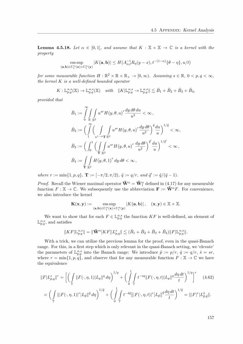
4.5 Appendix: Kernel Analysis
Lemma 4.5.18. Let α ∈ [0, 1], and assume that K : X × X → C is a kernel with theproperty
ess sup(a,b)∈Uα
1 (x)×Uα1 (y)
|Ka,b
| ≤ H
A−1
α,tRη(y − x), t−(1−α)θ − η, u/t
for some measurable function H : R2 × R × R+ → [0,∞). Assuming s ∈ R, 0 < p, q < ∞,the kernel K is a well-defined bounded operator
K : Lα,sp,q (X) → Lα,s
p,q (X) with ∥K|Lα,sp,q → Lα,s
p,q ∥ . B1 + B2 + B3 + B4,
provided that
B1 :=∞
0
R
R2
usrHy, θ, u
r dy dθ duu3 < ∞ ,
B2 := ∞
1
u1−αT
R2
usrHy, θ, u
r dy dθu2
q du
u
1/q
< ∞,
B3 := 1
0
T
R2
usrHy, θ, u
r dy dθu2
q′du
u
1/q′
< ∞ ,
B4 :=T
R2
Hy, θ, 1
rdy dθ < ∞ ,
where r := min1, p, q, T := [−π/2, π/2), q := q/r, and q′ := q/(q − 1).
Proof. Recall the Wiener maximal operator Wα = Wα1 defined in (4.17) for any measurable
function F : X → C. We subsequently use the abbreviation F := WαF . For convenience,we also introduce the kernel
K(x,y) := ess sup(a,b)∈Uα
1 (x)×Uα1 (y)
|Ka,b
| , (x,y) ∈ X × X.
We want to show that for each F ∈ Lα,sp,q the function KF is well-defined, an element of
Lα,sp,q , and satisfies
∥KF |Lα,sp,q ∥ = ∥Wα[KF ]|Ls
p,q∥ . (B1 + B2 + B3 + B4)∥F |Lα,sp,q ∥.
With a trick, we can utilize the previous lemma for the proof, even in the quasi-Banachrange. For this, in a first step which is only relevant in the quasi-Banach setting, we ‘elevate’the parameters of Lα,s
p,q into the Banach range: We introduce p := p/r, q := q/r, s = sr,where r = min1, p, q, and observe that for any measurable function F : X → C we havethe equivalence
∥F |Lsp,q∥r =
T
∥F (·, η, 1)|Lp∥q dη
1/q
+ 1
0
T
t−sq∥F (·, η, t)|Lp∥q dη dt
t
1/qr
(4.62)
≍
T
∥|F (·, η, 1)|r|Lp∥q dη
1/q
+ 1
0
T
t−sq|F (·, η, t)|r
Lp
q dη dt
t
1/q
= ∥|F |r|Lsp,q∥.
157
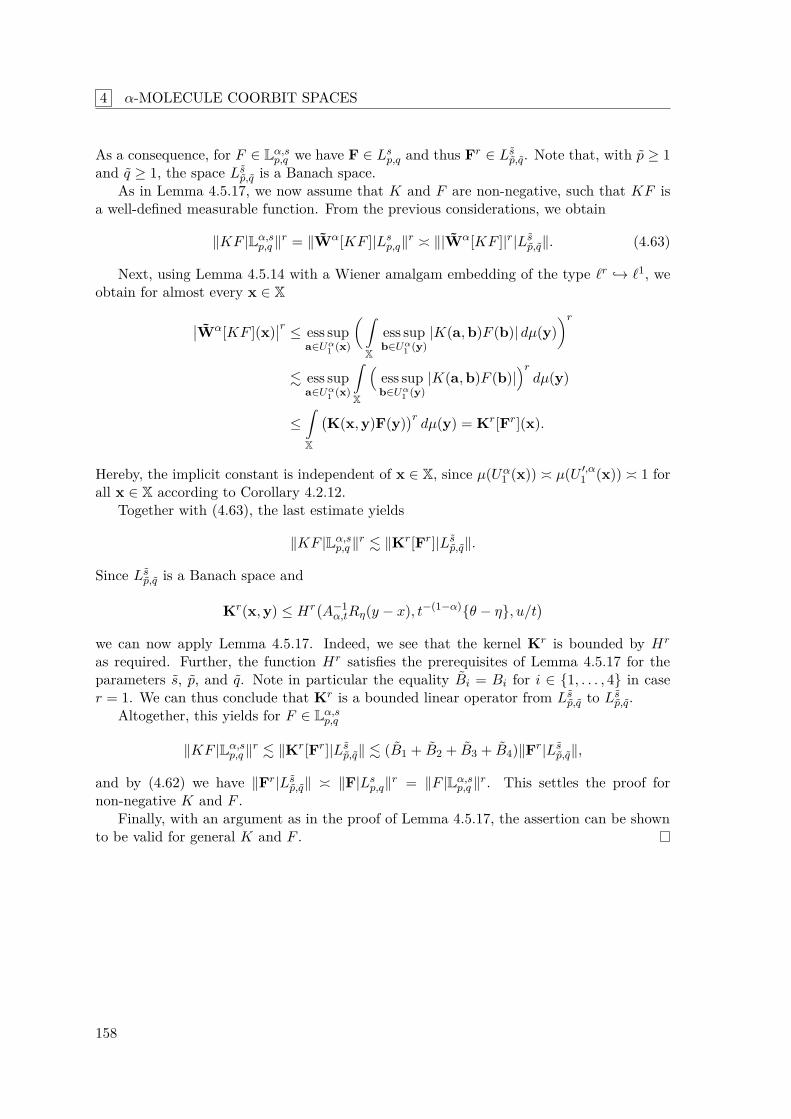
4 α-MOLECULE COORBIT SPACES
As a consequence, for F ∈ Lα,sp,q we have F ∈ Ls
p,q and thus Fr ∈ Lsp,q. Note that, with p ≥ 1
and q ≥ 1, the space Lsp,q is a Banach space.
As in Lemma 4.5.17, we now assume that K and F are non-negative, such that KF isa well-defined measurable function. From the previous considerations, we obtain
∥KF |Lα,sp,q ∥r = ∥Wα[KF ]|Ls
p,q∥r ≍ ∥|Wα[KF ]|r|Lsp,q∥. (4.63)
Next, using Lemma 4.5.14 with a Wiener amalgam embedding of the type ℓr → ℓ1, weobtain for almost every x ∈ X
Wα[KF ](x)r ≤ ess sup
a∈Uα1 (x)
X
ess supb∈Uα
1 (y)|K(a,b)F (b)| dµ(y)
r
. ess supa∈Uα
1 (x)
X
ess supb∈Uα
1 (y)|K(a,b)F (b)|
rdµ(y)
≤X
K(x,y)F(y)
rdµ(y) = Kr[Fr](x).
Hereby, the implicit constant is independent of x ∈ X, since µ(Uα1 (x)) ≍ µ(U ′,α
1 (x)) ≍ 1 forall x ∈ X according to Corollary 4.2.12.
Together with (4.63), the last estimate yields
∥KF |Lα,sp,q ∥r . ∥Kr[Fr]|Ls
p,q∥.
Since Lsp,q is a Banach space and
Kr(x,y) ≤ HrA−1α,tRη(y − x), t−(1−α)θ − η, u/t
we can now apply Lemma 4.5.17. Indeed, we see that the kernel Kr is bounded by Hr
as required. Further, the function Hr satisfies the prerequisites of Lemma 4.5.17 for theparameters s, p, and q. Note in particular the equality Bi = Bi for i ∈ 1, . . . , 4 in caser = 1. We can thus conclude that Kr is a bounded linear operator from Ls
p,q to Lsp,q.
Altogether, this yields for F ∈ Lα,sp,q
∥KF |Lα,sp,q ∥r . ∥Kr[Fr]|Ls
p,q∥ . (B1 + B2 + B3 + B4)∥Fr|Lsp,q∥,
and by (4.62) we have ∥Fr|Lsp,q∥ ≍ ∥F|Ls
p,q∥r = ∥F |Lα,sp,q ∥r. This settles the proof for
non-negative K and F .Finally, with an argument as in the proof of Lemma 4.5.17, the assertion can be shown
to be valid for general K and F .
158
Chapter 5
Cartoon Approximation withα-Molecules: Bounds
Many applications require efficient encoding of multivariate data in the sense of optimalsparse approximation. This is typically phrased as a problem of best N -term approximationwith respect to a suitable representation system as explained in Subsection 2.3.1.
In the following two chapters we are concretely interested in the performance of α-molecule systems for the sparse approximation of image data. As a model for the data,we will use the model of cartoon-like functions which very well captures the occurrence ofdiscontinuities such as edges in an image. Some guarantees for actually achievable N -termapproximation rates will be derived in the next chapter. In this chapter the focus is ontheoretical bounds limiting the maximally achievable approximation rates by α-molecules.
The presented research was conducted in [60] and [102]. At first, we study the approx-imability of cartoon-like data by arbitrary dictionaries under the assumption of a polyno-mial search depth. The main result, Theorem 5.3.3 ([60, Thm. 2.8]), will provide an upperbound for the achievable rates in this general setup. In Theorems 5.4.2 and 5.4.4 ([102,Thm. 3.9 & 3.11]), we then prove more specific bounds for the α-curvelet frame from Sub-section 3.2.3. Those also have implications for more general α-molecule frames, as derivedin Theorem 5.4.6 ([102, Thm. 5.3]).
5.1 Sparse Approximation Bounds
As in Subsection 2.3.1, we again begin with some abstract considerations in a separableHilbert space H. Assume that Φ = ϕλλ∈Λ is a dictionary in H and let ΣN := ΣN [Φ]be the associated space of N -term expansions introduced in (2.29). Further recall that theN -term approximation error (2.30) for a signal f ∈ H with respect to Φ is given by
σN (f) := infg∈ΣN
∥f − g∥.
To measure the approximation performance of Φ with respect of f , we will subsequentlyuse the asymptotic approximation rate, i.e., the decay of the approximation error σN (f)as N → ∞. For a subclass F ⊆ H, the approximation performance shall be judged bythe worst-case approximations, i.e., the worst decay rate of σN (f) for f ∈ F. In thissense, a dictionary Φ is considered optimal for sparse approximation of F, if its worst-caseapproximation rates for signals f ∈ F are the best among all systems.
Without reasonable restrictions, however, the investigation of the best N -term approxi-mation error with respect to a given dictionary can be meaningless for practical applications.For example, if Φ is chosen as a countable dense subset of H one would obtain arbitrarily
159
5 CARTOON APPROXIMATION WITH α-MOLECULES: BOUNDS
good 1-term approximations for every signal f ∈ H. This would translate to arbitrarilygood approximation rates, which clearly cannot be realized in practice.
For a proper assessment of the approximation performance of a dictionary, the actualapproximation scheme needs to be taken into account, i.e., the utilized process of selectingsuitable dictionary elements. A realistic assumption for such a selection procedure is aso-called polynomial depth search constraint, which requires that the terms of the N -termapproximations have to be selected from the first π(N) elements of the dictionary, where πis some fixed polynomial [38].
5.1.1 Polynomial Depth Search in a Dictionary
For the subsequent investigation, let us concretize our considered scenario. Assume that wehave a countable dictionary Φ = (ϕn)n∈N which without loss of generality is indexed by thenatural numbers. A non-linear N -term approximation scheme can then be described by aset-valued selection function S, which determines for given f ∈ H and N ∈ N the selecteddictionary elements, i.e., S(f,N) ⊂ Φ with #S(f,N) = N . Note that, due to the alloweddependence of S on f , by this general procedure even adaptive approximation schemescan be implemented. The obtained approximants are the elements fN ∈ span S(f,N)minimizing the error ∥f − fN ∥.
A polynomial depth search constraint for the selection rule S is described by a fixedpolynomial π and the condition S(f,N) ⊆ ϕ1, . . . , ϕπ(N) for all f ∈ H and N ∈ N. Underthis condition, an optimal selection S thus yields best N -term approximations fN ∈ ΣN inthe following modified sense,
fN = arg ming=
λ∈ΛNcλϕλ
∥f − g∥ s.t. ΛN ⊆ 1, . . . , π(N), #ΛN ≤ N. (5.1)
This definition of fN should be compared with (2.31). Whereas fN in the sense of (2.31)might not exist, the existence of fN as in (5.1) is always guaranteed.
We now recall a benchmark derived in [38] concerning the optimal approximation rateof a dictionary when polynomial depth search is used. Beforehand, we have to recall whatit means for a subclass F ⊆ H to contain a copy of ℓp0 (see also [38, Def. 1&2]).
Definition 5.1.1 ([60, Def. 2.2]). (i) A subclass F ⊆ H is said to contain an embeddedorthogonal hypercube of dimension m and sidelength δ if there exist f0 ∈ F and or-thogonal elements ψi ∈ H for i = 1, ...,m with ∥ψi∥ = δ such that the collection ofhypercube vertices
H(m; f0, (ψi)i) =h = f0 +
mi=1
ϵiψi : ϵi ∈ 0, 1
is contained in F. It should be noted that H just consists of its vertices.
(ii) A subclass F ⊆ H is said to contain a copy of ℓp0, p > 0, if there exists a sequenceof orthogonal hypercubes (Hk)k∈N, embedded in F, which have dimensions mk andsidelengths δk, such that δk → 0 and for some constant C > 0
mk ≥ Cδ−pk for all k ∈ N. (5.2)
160
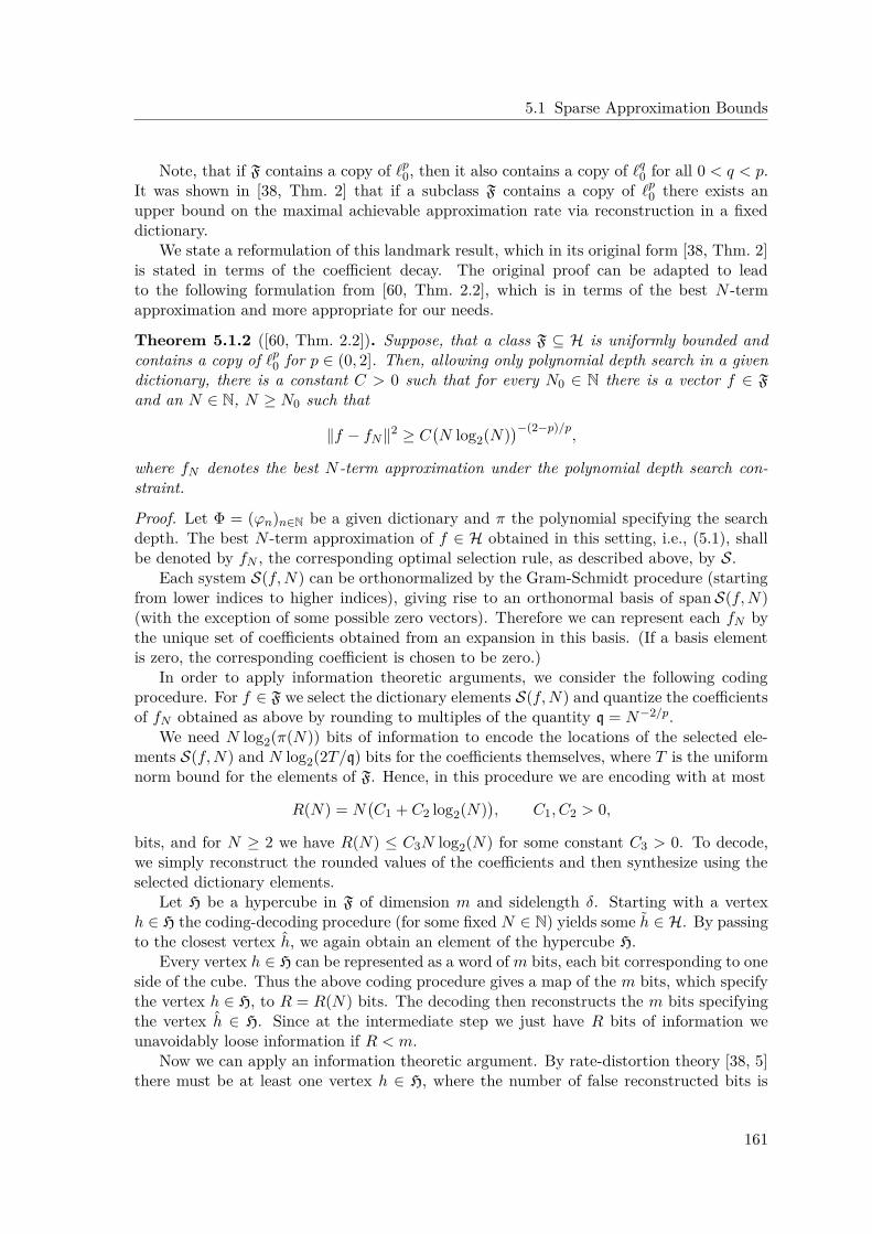
5.1 Sparse Approximation Bounds
Note, that if F contains a copy of ℓp0, then it also contains a copy of ℓq0 for all 0 < q < p.It was shown in [38, Thm. 2] that if a subclass F contains a copy of ℓp0 there exists anupper bound on the maximal achievable approximation rate via reconstruction in a fixeddictionary.
We state a reformulation of this landmark result, which in its original form [38, Thm. 2]is stated in terms of the coefficient decay. The original proof can be adapted to leadto the following formulation from [60, Thm. 2.2], which is in terms of the best N -termapproximation and more appropriate for our needs.
Theorem 5.1.2 ([60, Thm. 2.2]). Suppose, that a class F ⊆ H is uniformly bounded andcontains a copy of ℓp0 for p ∈ (0, 2]. Then, allowing only polynomial depth search in a givendictionary, there is a constant C > 0 such that for every N0 ∈ N there is a vector f ∈ Fand an N ∈ N, N ≥ N0 such that
∥f − fN ∥2 ≥ CN log2(N)
−(2−p)/p,
where fN denotes the best N -term approximation under the polynomial depth search con-straint.
Proof. Let Φ = (ϕn)n∈N be a given dictionary and π the polynomial specifying the searchdepth. The best N -term approximation of f ∈ H obtained in this setting, i.e., (5.1), shallbe denoted by fN , the corresponding optimal selection rule, as described above, by S.
Each system S(f,N) can be orthonormalized by the Gram-Schmidt procedure (startingfrom lower indices to higher indices), giving rise to an orthonormal basis of span S(f,N)(with the exception of some possible zero vectors). Therefore we can represent each fN bythe unique set of coefficients obtained from an expansion in this basis. (If a basis elementis zero, the corresponding coefficient is chosen to be zero.)
In order to apply information theoretic arguments, we consider the following codingprocedure. For f ∈ F we select the dictionary elements S(f,N) and quantize the coefficientsof fN obtained as above by rounding to multiples of the quantity q = N−2/p.
We need N log2(π(N)) bits of information to encode the locations of the selected ele-ments S(f,N) and N log2(2T/q) bits for the coefficients themselves, where T is the uniformnorm bound for the elements of F. Hence, in this procedure we are encoding with at most
R(N) = NC1 + C2 log2(N)
, C1, C2 > 0,
bits, and for N ≥ 2 we have R(N) ≤ C3N log2(N) for some constant C3 > 0. To decode,we simply reconstruct the rounded values of the coefficients and then synthesize using theselected dictionary elements.
Let H be a hypercube in F of dimension m and sidelength δ. Starting with a vertexh ∈ H the coding-decoding procedure (for some fixed N ∈ N) yields some h ∈ H. By passingto the closest vertex h, we again obtain an element of the hypercube H.
Every vertex h ∈ H can be represented as a word of m bits, each bit corresponding to oneside of the cube. Thus the above coding procedure gives a map of the m bits, which specifythe vertex h ∈ H, to R = R(N) bits. The decoding then reconstructs the m bits specifyingthe vertex h ∈ H. Since at the intermediate step we just have R bits of information weunavoidably loose information if R < m.
Now we can apply an information theoretic argument. By rate-distortion theory [38, 5]there must be at least one vertex h ∈ H, where the number of false reconstructed bits is
161
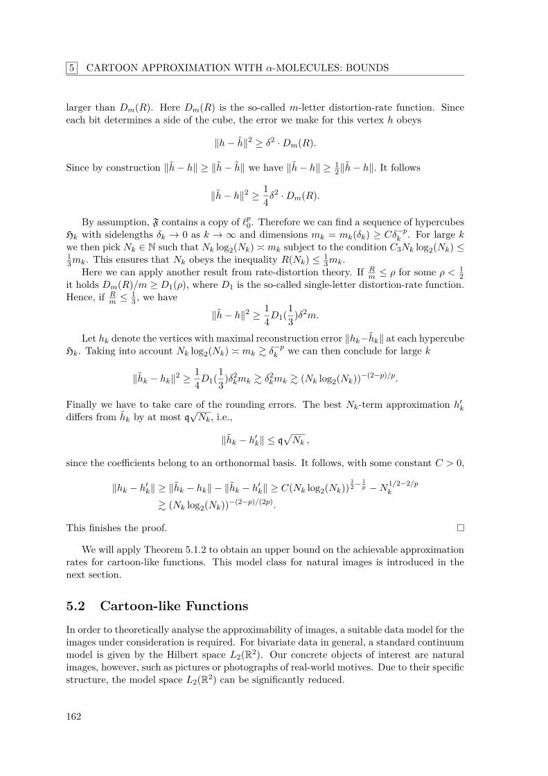
5 CARTOON APPROXIMATION WITH α-MOLECULES: BOUNDS
larger than Dm(R). Here Dm(R) is the so-called m-letter distortion-rate function. Sinceeach bit determines a side of the cube, the error we make for this vertex h obeys
∥h− h∥2 ≥ δ2 ·Dm(R).
Since by construction ∥h− h∥ ≥ ∥h− h∥ we have ∥h− h∥ ≥ 12∥h− h∥. It follows
∥h− h∥2 ≥ 14δ
2 ·Dm(R).
By assumption, F contains a copy of ℓp0. Therefore we can find a sequence of hypercubesHk with sidelengths δk → 0 as k → ∞ and dimensions mk = mk(δk) ≥ Cδ−p
k . For large kwe then pick Nk ∈ N such that Nk log2(Nk) ≍ mk subject to the condition C3Nk log2(Nk) ≤13mk. This ensures that Nk obeys the inequality R(Nk) ≤ 1
3mk.Here we can apply another result from rate-distortion theory. If R
m ≤ ρ for some ρ < 12
it holds Dm(R)/m ≥ D1(ρ), where D1 is the so-called single-letter distortion-rate function.Hence, if R
m ≤ 13 , we have
∥h− h∥2 ≥ 14D1(1
3)δ2m.
Let hk denote the vertices with maximal reconstruction error ∥hk−hk∥ at each hypercubeHk. Taking into account Nk log2(Nk) ≍ mk & δ−p
k we can then conclude for large k
∥hk − hk∥2 ≥ 14D1(1
3)δ2kmk & δ2
kmk & (Nk log2(Nk))−(2−p)/p.
Finally we have to take care of the rounding errors. The best Nk-term approximation h′k
differs from hk by at most q√Nk, i.e.,
∥hk − h′k∥ ≤ q
Nk ,
since the coefficients belong to an orthonormal basis. It follows, with some constant C > 0,
∥hk − h′k∥ ≥ ∥hk − hk∥ − ∥hk − h′
k∥ ≥ C(Nk log2(Nk))12 − 1
p −N1/2−2/pk
& (Nk log2(Nk))−(2−p)/(2p).
This finishes the proof.
We will apply Theorem 5.1.2 to obtain an upper bound on the achievable approximationrates for cartoon-like functions. This model class for natural images is introduced in thenext section.
5.2 Cartoon-like Functions
In order to theoretically analyse the approximability of images, a suitable data model for theimages under consideration is required. For bivariate data in general, a standard continuummodel is given by the Hilbert space L2(R2). Our concrete objects of interest are naturalimages, however, such as pictures or photographs of real-world motives. Due to their specificstructure, the model space L2(R2) can be significantly reduced.
162
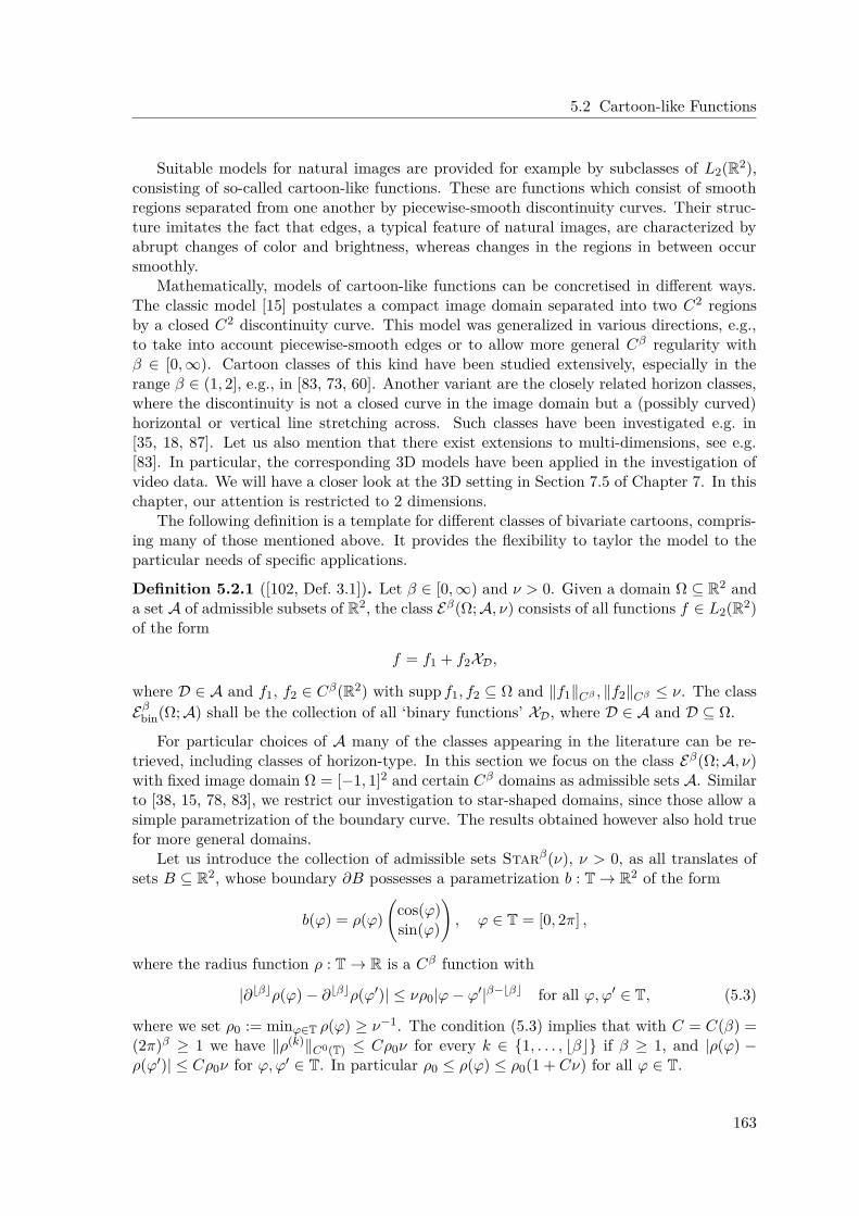
5.2 Cartoon-like Functions
Suitable models for natural images are provided for example by subclasses of L2(R2),consisting of so-called cartoon-like functions. These are functions which consist of smoothregions separated from one another by piecewise-smooth discontinuity curves. Their struc-ture imitates the fact that edges, a typical feature of natural images, are characterized byabrupt changes of color and brightness, whereas changes in the regions in between occursmoothly.
Mathematically, models of cartoon-like functions can be concretised in different ways.The classic model [15] postulates a compact image domain separated into two C2 regionsby a closed C2 discontinuity curve. This model was generalized in various directions, e.g.,to take into account piecewise-smooth edges or to allow more general Cβ regularity withβ ∈ [0,∞). Cartoon classes of this kind have been studied extensively, especially in therange β ∈ (1, 2], e.g., in [83, 73, 60]. Another variant are the closely related horizon classes,where the discontinuity is not a closed curve in the image domain but a (possibly curved)horizontal or vertical line stretching across. Such classes have been investigated e.g. in[35, 18, 87]. Let us also mention that there exist extensions to multi-dimensions, see e.g.[83]. In particular, the corresponding 3D models have been applied in the investigation ofvideo data. We will have a closer look at the 3D setting in Section 7.5 of Chapter 7. In thischapter, our attention is restricted to 2 dimensions.
The following definition is a template for different classes of bivariate cartoons, compris-ing many of those mentioned above. It provides the flexibility to taylor the model to theparticular needs of specific applications.
Definition 5.2.1 ([102, Def. 3.1]). Let β ∈ [0,∞) and ν > 0. Given a domain Ω ⊆ R2 anda set A of admissible subsets of R2, the class Eβ(Ω; A, ν) consists of all functions f ∈ L2(R2)of the form
f = f1 + f2XD,
where D ∈ A and f1, f2 ∈ Cβ(R2) with supp f1, f2 ⊆ Ω and ∥f1∥Cβ , ∥f2∥Cβ ≤ ν. The classEβ
bin(Ω; A) shall be the collection of all ‘binary functions’ XD, where D ∈ A and D ⊆ Ω.
For particular choices of A many of the classes appearing in the literature can be re-trieved, including classes of horizon-type. In this section we focus on the class Eβ(Ω; A, ν)with fixed image domain Ω = [−1, 1]2 and certain Cβ domains as admissible sets A. Similarto [38, 15, 78, 83], we restrict our investigation to star-shaped domains, since those allow asimple parametrization of the boundary curve. The results obtained however also hold truefor more general domains.
Let us introduce the collection of admissible sets Starβ(ν), ν > 0, as all translates ofsets B ⊆ R2, whose boundary ∂B possesses a parametrization b : T → R2 of the form
b(ϕ) = ρ(ϕ)
cos(ϕ)sin(ϕ)
, ϕ ∈ T = [0, 2π] ,
where the radius function ρ : T → R is a Cβ function with
|∂⌊β⌋ρ(ϕ) − ∂⌊β⌋ρ(ϕ′)| ≤ νρ0|ϕ− ϕ′|β−⌊β⌋ for all ϕ,ϕ′ ∈ T, (5.3)
where we set ρ0 := minϕ∈T ρ(ϕ) ≥ ν−1. The condition (5.3) implies that with C = C(β) =(2π)β ≥ 1 we have ∥ρ(k)∥C0(T) ≤ Cρ0ν for every k ∈ 1, . . . , ⌊β⌋ if β ≥ 1, and |ρ(ϕ) −ρ(ϕ′)| ≤ Cρ0ν for ϕ,ϕ′ ∈ T. In particular ρ0 ≤ ρ(ϕ) ≤ ρ0(1 + Cν) for all ϕ ∈ T.
163
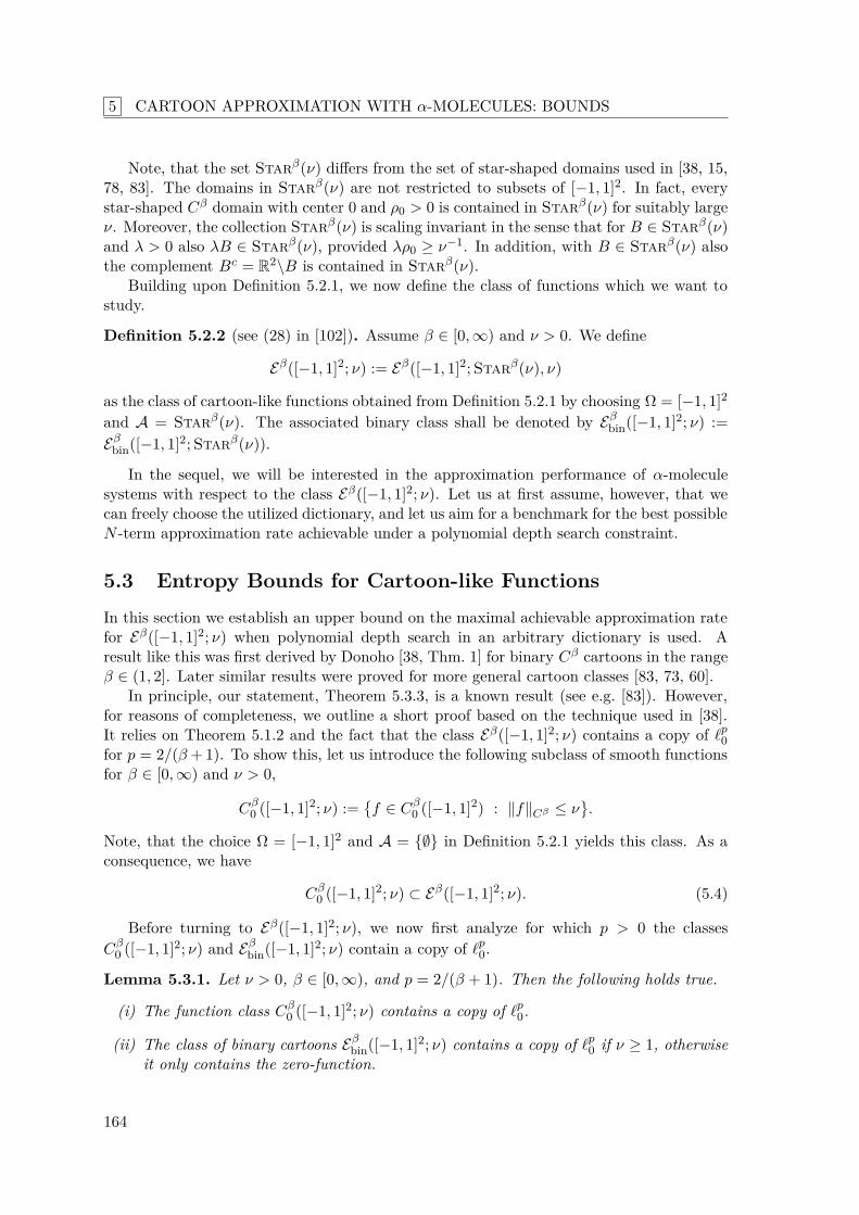
5 CARTOON APPROXIMATION WITH α-MOLECULES: BOUNDS
Note, that the set Starβ(ν) differs from the set of star-shaped domains used in [38, 15,78, 83]. The domains in Starβ(ν) are not restricted to subsets of [−1, 1]2. In fact, everystar-shaped Cβ domain with center 0 and ρ0 > 0 is contained in Starβ(ν) for suitably largeν. Moreover, the collection Starβ(ν) is scaling invariant in the sense that for B ∈ Starβ(ν)and λ > 0 also λB ∈ Starβ(ν), provided λρ0 ≥ ν−1. In addition, with B ∈ Starβ(ν) alsothe complement Bc = R2\B is contained in Starβ(ν).
Building upon Definition 5.2.1, we now define the class of functions which we want tostudy.
Definition 5.2.2 (see (28) in [102]). Assume β ∈ [0,∞) and ν > 0. We define
Eβ([−1, 1]2; ν) := Eβ([−1, 1]2; Starβ(ν), ν)
as the class of cartoon-like functions obtained from Definition 5.2.1 by choosing Ω = [−1, 1]2and A = Starβ(ν). The associated binary class shall be denoted by Eβ
bin([−1, 1]2; ν) :=Eβ
bin([−1, 1]2; Starβ(ν)).
In the sequel, we will be interested in the approximation performance of α-moleculesystems with respect to the class Eβ([−1, 1]2; ν). Let us at first assume, however, that wecan freely choose the utilized dictionary, and let us aim for a benchmark for the best possibleN -term approximation rate achievable under a polynomial depth search constraint.
5.3 Entropy Bounds for Cartoon-like Functions
In this section we establish an upper bound on the maximal achievable approximation ratefor Eβ([−1, 1]2; ν) when polynomial depth search in an arbitrary dictionary is used. Aresult like this was first derived by Donoho [38, Thm. 1] for binary Cβ cartoons in the rangeβ ∈ (1, 2]. Later similar results were proved for more general cartoon classes [83, 73, 60].
In principle, our statement, Theorem 5.3.3, is a known result (see e.g. [83]). However,for reasons of completeness, we outline a short proof based on the technique used in [38].It relies on Theorem 5.1.2 and the fact that the class Eβ([−1, 1]2; ν) contains a copy of ℓp0for p = 2/(β+ 1). To show this, let us introduce the following subclass of smooth functionsfor β ∈ [0,∞) and ν > 0,
Cβ0 ([−1, 1]2; ν) :=
f ∈ Cβ
0 ([−1, 1]2) : ∥f∥Cβ ≤ ν.
Note, that the choice Ω = [−1, 1]2 and A = ∅ in Definition 5.2.1 yields this class. As aconsequence, we have
Cβ0 ([−1, 1]2; ν) ⊂ Eβ([−1, 1]2; ν). (5.4)
Before turning to Eβ([−1, 1]2; ν), we now first analyze for which p > 0 the classesCβ
0 ([−1, 1]2; ν) and Eβbin([−1, 1]2; ν) contain a copy of ℓp0.
Lemma 5.3.1. Let ν > 0, β ∈ [0,∞), and p = 2/(β + 1). Then the following holds true.
(i) The function class Cβ0 ([−1, 1]2; ν) contains a copy of ℓp0.
(ii) The class of binary cartoons Eβbin([−1, 1]2; ν) contains a copy of ℓp0 if ν ≥ 1, otherwise
it only contains the zero-function.
164

5.3 Entropy Bounds for Cartoon-like Functions
Proof. The proof is a 2D-adaption of the proof of [83, Thm. 3.2].Part (i): Let φ ∈ C∞
0 (R) with suppφ ⊆ [0, 1] and φ ≥ 0 and put ψ(t) = φ(t1)φ(t2) fort = (t1, t2) ∈ R2. Then ψ ∈ C∞(R2) with suppψ ⊆ [0, 1]2. We choose φ = 0 such that∥ψ∥Cβ(R2) ≤ ν. Next, we define for k ∈ N and ℓ = (ℓ1, ℓ2) ∈ 0, ..., k − 12 the functions
ψk,ℓ(t) = k−βφ(kt1 − ℓ1)φ(kt2 − ℓ2).
These functions ψk,ℓ ∈ C∞(R2) are dilated and translated versions of ψ with suppψk,ℓ ⊆[ ℓ1
k ,ℓ1+1
k ] × [ ℓ2k ,
ℓ2+1k ] and ∥ψk,ℓ∥Cβ(R2) ≤ ∥ψ∥Cβ(R2) ≤ ν. In particular, ψk,ℓ and ψk,ℓ′ are
orthogonal in L2(R2) if ℓ = ℓ′. The functions in the set
Hk :=
ℓ∈0,...,k−12
ϵℓψk,ℓ : ϵℓ ∈ 0, 1 for every ℓ ∈ 0, . . . , k − 12
constitute the vertices of an orthogonal hypercube of dimension mk = k2 and side-lengthδk = ∥ψk,ℓ∥2 = k−β−1∥ψ∥2, which is embedded in the class Cβ
0 ([−1, 1]2; ν). The sequence(δk)k∈N obeys δk → 0 as k → ∞. Further (5.2) is fulfilled with p = 2/(β + 1) since
mk = k2 = (δk/∥ψ∥2)− 2β+1 = ∥ψ∥
2β+12 · (δk)− 2
β+1 .
Part (ii): We start with a function φ0 ∈ C∞(R) and assume suppφ0 ⊆ [0, π/4], 0 ≤ φ0 ≤cos(π/8)−1 − 1, and ∥φ0∥Cβ(R) = 1. Then we define for k ∈ N and ℓ ∈ 0, ..., k − 1 thefunctions
φk,ℓ(t) = k−βφ0(kt− ℓπ/4),
which clearly satisfy ∥φk,ℓ∥Cβ(R) ≤ ∥φ0∥Cβ(R) = 1. Moreover, they have the property∥φk,ℓ∥C0(R) ≤ k−β(cos(π/8)−1 − 1) and ∥φk,ℓ∥1 = k−β−1∥φ0∥1.
Next, we define the functions ρk,ℓ ∈ C∞(T) on the torus T = [0, 2π) via ρk,ℓ(t) =1 + φk,ℓ(t− π/8). They satisfy 1 ≤ ρk,ℓ ≤ cos(π/8)−1, such that Dk,ℓ ⊂ [−1, 1]2 for the sets
Dk,ℓ :=x ∈ R2 : x = (r, ϕ) in polar coordinates with 1 < r ≤ ρk,ℓ(ϕ), ϕ ∈ T
.
For fixed k, the characteristic functions ψk,ℓ := XDk,ℓare mutually orthogonal in L2(R2)
due to their disjoint support. Let B2(0, 1) denote the unit ball in R2 and consider theorthogonal hypercubes Hk of dimension mk = k and side-length δk = ∥ψk,ℓ∥2 given by
Hk :=
XB2(0,1) +
ℓ∈0,...,k−1ϵℓψk,ℓ : ϵ = (ϵ1, . . . , ϵk−1) ∈ 0, 1k−1
.
If ν ≥ 1 those are contained in Eβbin([−1, 1]2; ν). Moreover, since 0 ≤ ∥φk,ℓ∥2
2 ≤ ∥φk,ℓ∥1, itholds
∥ψk,ℓ∥22 =
2π
0
∞
0|ψk,ℓ(r, ϕ)|r drdϕ =
2π
0
1+φk,ℓ(ϕ)
1r drdϕ = ∥φk,ℓ∥1 + 1
2∥φk,ℓ∥22 ≍ ∥φk,ℓ∥1.
This implies δk ≍ k−(β+1)/2 → 0 for k → ∞ and (5.2) with p = 2/(β + 1) since mk = k ≍(δk)− 2
β+1 .
165
5 CARTOON APPROXIMATION WITH α-MOLECULES: BOUNDS
As a consequence of (5.4), we can deduce from Lemma 5.3.1(i) that also Eβ([−1, 1]2; ν)contains a copy of ℓ2/(β+1)
0 .
Corollary 5.3.2. The function class Eβ([−1, 1]2; ν) contains a copy of ℓp0 for p = 2/(β+1).
An application of Theorem 5.1.2 thus yields Theorem 5.3.3 below.
Theorem 5.3.3 (compare [83]). Let β, γ ∈ [0,∞) and ν > 0. Assume that there is aconstant C > 0 such that
supf∈Eβ([−1,1]2;ν)
∥f − fN ∥22 ≤ CN−γ for all N ∈ N,
where fN denotes the best N -term approximation of f obtained by polynomial depth searchin a fixed dictionary. Then necessarily γ ≤ β.
The optimality benchmark N−β is also valid for Cβ0 ([−1, 1]2; ν) and Eβ
bin([−1, 1]2; ν) withν ≥ 1. We end this section with this observation.
Remark 5.3.4. According to Lemma 5.3.1(i), the bound of Theorem 5.3.3 even holds truefor the class Cβ
0 ([−1, 1]2; ν). This is a stronger statement due to the inclusion (5.4). Further,due to Lemma 5.3.1(ii), a statement analogous to Theorem 5.3.3 holds true for the binaryclass Eβ
bin([−1, 1]2; ν) if ν ≥ 1.
5.4 Approximation Bounds for α-Molecule Systems
Whereas the subject of the previous section was the approximability of the set Eβ([−1, 1]2; ν)by general dictionaries, we are now more specifically interested in the approximation α-molecule systems can provide. In the subsequent investigation, which was first conductedin [102], we will analyze the approximation performance of the discrete Parseval frame ofα-curvelets C•
α from Subsection 3.2.3. As shown by Proposition 3.2.8, this frame is a systemof α-molecules of order (∞,∞,∞,∞), which makes it a suitable anchor system for theapplication of the transfer principle, Theorem 2.3.6. Hence, the bounds we will obtain inTheorem 5.4.2 ([102, Thm. 3.9]) and Theorem 5.4.4 ([102, Thm. 3.11]) for the achievablerates of C•
α also have consequences for other α-molecule systems. These will be stated inTheorem 5.4.6 ([102, Thm. 5.3]).
5.4.1 The Anchor System: α-Curvelets
Before our investigation of approximation properties, let us shortly revisit the constructionof the frame C•
α = ψµµ∈M from Subsection 3.2.3. First, recall that its index set M is ofthe form M = J × Z2 with
J :=J = (j, ℓ) : j ∈ N0, ℓ ∈ 0, . . . , Lj − 1
and
Lj = 2⌊j(1−α)⌋ , j ∈ N0. (5.5)
166
5.4 Approximation Bounds for α-Molecule Systems
Next, recall that the functions ψj,ℓ,k ∈ C•α are simply rotations and translations of the
α-curvelets ψj,0,0. Let Rη denote the rotation matrix (2.3) and Aα,t the α-scaling matrix(2.4), i.e.,
Rη =
cos(η) − sin(η)sin(η) cos(η)
and Aα,t =
t 00 tα
, η ∈ R, t ∈ R+.
Then, according to (3.23), for every (j, ℓ, k) ∈ M we have the relation
ψj,ℓ,k(·) = ψj,0,0Rℓωj
· −A−1α,2jk
,
where ωj is the angle
ωj = πL−1j = π2−⌊j(1−α)⌋ , j ∈ N0.
Finally, recall that the Fourier representation of ψj,ℓ,k ∈ C•α is given by
ψj,ℓ,k(ξ) = Wj,ℓ(ξ)uj,ℓ,k(ξ) , ξ ∈ R2,
where Wj,ℓ : R2 → [0, 1] is a wedge function as in (3.18) and uj,ℓ,k = uj,0,k(Rℓωj·) is obtained
by rotating the exponential
uj,0,k(ξ) = 2−j(1+α)/2 exp2πi(2−jk1ξ1 + 2−jαk2ξ2)
, ξ = (ξ1, ξ2) ∈ R2.
We will now elaborate a bit on the geometric aspects of the frequency tiling inducedby C•
α. Clearly, it is determined by the support of the functions WJ ∈ C∞0 (R2) which,
according to their definition (3.18), are polar tensor products of respective radial and angularcomponents. For each J = (j, ℓ) ∈ J we have
Wj,ℓ(ξ) = Uj(|ξ|2)Vj,ℓ(ξ/|ξ|2), ξ ∈ R2, (5.6)
with a radial function Uj ∈ C∞(R+0 , [0, 1]) and an angular function Vj,ℓ ∈ C∞(S1, [0, 1]).
The functions Uj ∈ C∞(R+0 ), j ∈ N0, satisfy the support condition suppUj ⊆ Ij ,
whereby
I0 := 16π · [0, 2] and Ij := 1
6π · [2j−1, 2j+1] , j ≥ 1. (5.7)
Further, due to (3.15) and (3.16), they equal 1 on the respective intervals
I−0 := 1
6π · [0, τ1] and I−j := 1
6π · [2j−1τ2, 2jτ1], j ≥ 1. (5.8)
As a consequence, all functions WJ belonging to a fixed scale j ∈ N0 have support in acorona Cj defined by C0 := ξ ∈ R2 : 6π|ξ|2 ≤ 2 for j = 0 and
Cj :=ξ ∈ R2 : 2j−1 ≤ 6π|ξ|2 ≤ 2j+1
, for j ≥ 1.
More concretely, taking into account the support of the functions Vj,ℓ, the approximatesupport of Wj,ℓ corresponds to a pair of opposite wedges Wj,ℓ := R−1
ℓωjWj,0, which is obtained
as a rotation of the set
Wj,0 :=ξ = (ξ1, ξ2) ∈ Cj : |ξ1| ≥ cos(ϕj/2)|ξ|2
.
167
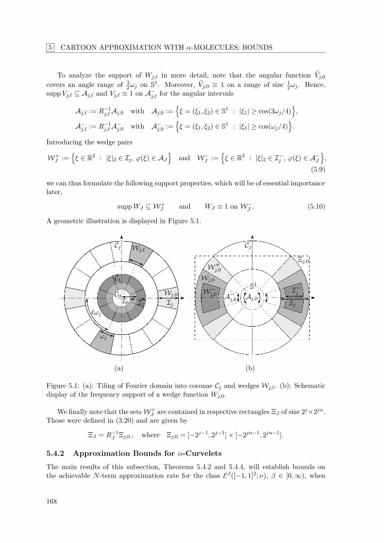
5 CARTOON APPROXIMATION WITH α-MOLECULES: BOUNDS
To analyze the support of Wj,ℓ in more detail, note that the angular function Vj,0covers an angle range of 3
2ωj on S1. Moreover, Vj,0 ≡ 1 on a range of size 12ωj . Hence,
suppVj,ℓ ⊆ Aj,ℓ and Vj,ℓ ≡ 1 on A−j,ℓ for the angular intervals
Aj,ℓ := R−1j,ℓ Aj,0 with Aj,0 :=
ξ = (ξ1, ξ2) ∈ S1 : |ξ1| ≥ cos(3ωj/4)
,
A−j,ℓ := R−1
j,ℓ A−j,0 with A−
j,0 :=ξ = (ξ1, ξ2) ∈ S1 : |ξ1| ≥ cos(ωj/4)
.
Introducing the wedge pairs
W+J :=
ξ ∈ R2 : |ξ|2 ∈ Ij , ϕ(ξ) ∈ AJ
and W−
J :=ξ ∈ R2 : |ξ|2 ∈ I−
j , ϕ(ξ) ∈ A−J
,
(5.9)
we can thus formulate the following support properties, which will be of essential importancelater,
suppWJ ⊆ W+J and WJ ≡ 1 on W−
J . (5.10)
A geometric illustration is displayed in Figure 5.1.
C0I0
C1
I1
...
Cj
Wj,0Ij
Wj,ℓ
ωj
ℓωj
(a)
Wj,0
W+j,0
W−j,0
Ξj,0
Cj
S1
Aj,0A−j,0
I−j
Ij
(b)
Figure 5.1: (a): Tiling of Fourier domain into coronae Cj and wedges Wj,ℓ. (b): Schematicdisplay of the frequency support of a wedge function Wj,0.
We finally note that the sets W+J are contained in respective rectangles ΞJ of size 2j×2jα.
Those were defined in (3.20) and are given by
ΞJ = R−1J Ξj,0 , where Ξj,0 = [−2j−1, 2j−1] × [−2jα−1, 2jα−1].
5.4.2 Approximation Bounds for α-Curvelets
The main results of this subsection, Theorems 5.4.2 and 5.4.4, will establish bounds onthe achievable N -term approximation rate for the class Eβ([−1, 1]2; ν), β ∈ [0,∞), when
168
5.4 Approximation Bounds for α-Molecule Systems
using the α-curvelet frame C•α for approximation. Unlike the more general bounds in The-
orem 5.3.3, these bounds are tied to the particular approximation system C•α. They are
established by studying the approximability of certain example cartoons.We choose the characteristic function of the ball B2(0, 1
2) ⊂ R2 of radius 12 , for which
we subsequently use the symbol
Θ(x) := XB2(0, 12 )(x1, x2) , x ∈ R2. (5.11)
This function embodies an exceptionally regular binary cartoon. Its boundary is a closedC∞-curve. It is radial symmetric and contained in Eβ
bin([−1, 1]2, ν) for arbitrary β ∈ [0,∞)and ν ≥ 2. Furthermore, for every β ∈ [0,∞) and ν ≥ 2 there is γ > 0 such that γΘ ∈Eβ([−1, 1]2; ν), wherefore the approximability of Θ has implications for the approximabilityof these cartoon classes.
The Fourier transform of Θ is explicitly computable. Let J1 denote the Bessel functionof order 1, then according to (5.21)
Θ(ξ) = J1(π|ξ|)2|ξ|
, ξ ∈ R2. (5.12)
Some properties of J1 and Bessel functions in general are collected in the appendix, Sec-tion 5.5.
At the center of the following investigation is the lemma below, which estimates theenergy of Θ contained in the wedges WJ , J ∈ J. Let WJJ∈J be a family of wedgefunctions of the kind (3.18) with property (3.17). Further, let
W−J := XW−
Jand W+
J := XW+J
be the characteristic functions of the sets W−J and W+
J defined in (5.9).
Lemma 5.4.1 ([102, Lem. 3.8]). There are constants 0 < C1 ≤ C2 < ∞, independent ofscale j ≥ j0, where j0 ∈ N0 is a suitable base scale, such that for all J ∈ J with |J | ≥ j0
C12−j(2−α) ≤ ∥ΘW−J ∥2
2 ≤ ∥ΘWJ∥22 ≤ ∥ΘW+
J ∥22 ≤ C22−j(2−α),
whereby |J | = j for J = (j, ℓ) ∈ J.
Proof. Let us recall the Bessel function J1 of order 1 and its asymptotic behavior. Accordingto (5.23) there is a constant C > 0 and a function R1 on [1,∞) satisfying |R1(r)| ≤ Cr−3/2
such that
J1(r) =
2πr
cos(r − 3π4 ) +R1(r) for r ≥ 1.
This allows to separate terms of higher order from J 21 . We decompose
J 21 (r) =
2π
cos2(r − 3π4 )r−1
+ 8
πcos(r − 3π
4 )r−1/2R1(r) +R1(r)2
=: T1(r) + T2(r).
For the following argumentation we need the square wave function ⊓ : R → 0, 1 definedby
⊓(r) :=
1 , r ∈
k∈Z kπ + [−π2 , 0],
0 , r ∈
k∈Z kπ + (0, π2 ).
169
5 CARTOON APPROXIMATION WITH α-MOLECULES: BOUNDS
For all r ∈ R it has the property 2 cos2(r − 3π/4) ≥ ⊓(r). Therefore we can deduce for1 ≤ a ≤ b b
aT1(r)r−1 dr = 1
π
b
a2 cos2(r − 3π
4 )r−2 dr ≥ 1π
b
a⊓(r)r−2 dr ≥ 1
2
k∈Ia,b
(kπ)−2
with Ia,b := k ∈ Z : kπ ∈ [a+ π, b]. To proceed, we use the relationn
k=m
(kπ)−2 ≥ 1π
(n+1)π
mπk−2 dk,
which is valid for all m,n ∈ N and m ≤ n. We obtain
12
k∈Ia,b
(kπ)−2 ≥ 12π
b
a+2πk−2 dk = 1
2π b
ak−2 dk −
a+2π
ak−2 dk
≥ 1
2π (a−1 − b−1) − a−2.
Next, we see that with a constant C > 0 independent of 1 ≤ a ≤ b b
a|T2(r)|r−1 dr ≤ C
b
ar−3 dr ≤ C
∞
ar−3 dr ≤ Ca−2.
Altogether, we conclude that b
a
J 21 (r)r
dr ≥ 12π (1 − ab−1)a−1 − (1 + C)a−2.
If c = ab−1 ≤ 1 is fixed, we can deduce for a ≥ 4π 1+C1−c the estimate a/c
a
J 21 (r)r
dr ≥ 14π (1 − c)a−1. (5.13)
After this preparation, we can now turn to the actual proof of the assertion. The relation
∥ΘW−J ∥2
2 ≤ ∥ΘWJ∥22 ≤ ∥ΘW+
J ∥22
is a direct consequence of (5.10) and ∥WJ∥∞ ≤ 1. Let Ij be the intervals defined in (5.7).Further, recall the intervals I−
j ⊂ Ij defined in (5.8). Using (5.12) and the definition (5.9)of W−
J we calculate
∥ΘW−J ∥2
2 =
W−J
J 21 (π|ξ|)4|ξ|2
dξ =
I−j
A−
J
J 21 (πr)4r dϕdr ≍ 2−j(1−α)
πI−
j
J 21 (r)r
dr.
The intervals I−j scale like ∼ 2j . Hence, if j ∈ N is chosen large enough by (5.13)
∥ΘW−J ∥2
2 ≍ 2−j(1−α)
πI−j
J 21 (r)r−1 dr & 2−j(1−α)2−j = 2−j(2−α).
The estimate from above is much easier to establish. If j ∈ N such that πIj ⊂ [1,∞) wehave
∥ΘW+J ∥2
2 =
W+J
J 21 (π|ξ|)4|ξ|2
dξ =
Ij
AJ
J 21 (πr)4r dϕdr ≍ 2−j(1−α)
πIj
J 21 (r)r
dr
. 2−j(1−α)
Ij
r−2 dr . 2−j(2−α).
170
5.4 Approximation Bounds for α-Molecule Systems
Based on Lemma 5.4.1 we can prove the first main result of this subsection.
Theorem 5.4.2 ([102, Thm. 3.9]). Let C•α be the α-curvelet frame constructed in Subsec-
tion 3.2.3 for fixed α ∈ [0, 1). There exists a constant C > 0 such that for any given N ∈ Nevery N -term approximation fN of Θ with respect to C•
α (not even subject to a polynomialdepth search constraint) satisfies
∥Θ − fN ∥22 ≥ CN− 1
1−α .
Proof. Let N ∈ N be fixed and assume that
fN =N
r=1θJr,krψJr,kr
is a linear combination of α-curvelets ψJr,kr with coefficients θJr,kr ∈ R. The curveletsψJr,kr ∈ C•
α satisfy supp ψJr,kr ⊆ W+Jr
as recorded in (5.10). It follows supp fN ⊆ WN
where WN :=
J∈JNW+
J for JN := J1, . . . , JN ⊂ J. Using the notation JcN := J\JN and
WcN := R2\WN we get with Lemma 5.4.1
∥Θ − fN ∥22 = ∥Θ − fN ∥2
2 ≥ ∥Θ∥2L2(Wc
N ) ≥
J∈JcN
∥ΘW−J ∥2
2 &
J∈JcN
2−j(2−α).
We want to bound the right-hand side from below. By (5.5), the number of tiles in eachcorona Cj , j ∈ N0, is given by Lj , where Lj = 2⌊j(1−α)⌋ for j ∈ N0. Let j(N) ∈ N denotethe unique number such that
j(N)−1j=0
Lj < N ≤j(N)j=0
Lj .
Since 2−j(2−α) decreases with rising scale we obtain
J∈Jc
N
2−j(2−α) ≥∞
j=j(N)+1Lj2−j(2−α) ≥ 1
2
∞j=j(N)+1
2−j & 2−j(N).
Here we used Lj ≥ 2j(1−α)−1. Since N &j(N)−1
j=0 2j(1−α) & 2j(N)(1−α) we can finally deduce
∥Θ − fN ∥22 & 2−j(N) =
2j(N)(1−α)
− 11−α
& N− 11−α .
This result can be strengthened if we restrict to greedy N -term approximations obtainedby thresholding the coefficients. Essential is the following observation, which has also beenused in [60]. Due to its importance we give a rigorous proof here.
Lemma 5.4.3 ([102, Lem. 3.10]). There is a constant C > 0 such that all curvelets ψµ ∈ C•α,
µ ∈ M , satisfy∥ψµ∥1 ≤ C2−j(1+α)/2.
171
5 CARTOON APPROXIMATION WITH α-MOLECULES: BOUNDS
Proof. Let aj be the functions from (3.25) and recall that according to (3.27) the support ofaj is contained in the unit square Ξ0,0 for every j ∈ N0. Let Id denote the identity operator.We have the estimateF−1
(Id + ∂2
1)(Id + ∂22)aj
∞
≤ ∥(Id + ∂21)(Id + ∂2
2)aj∥1 ≤ ∥(Id + ∂21)(Id + ∂2
2)aj∥∞.
According to Proposition 3.2.8(ii) the right-hand side is bounded uniformly over all scales.We conclude that there is a constant C > 0, independent of j ∈ N0, such that
supx∈R2
|(1 + x21)(1 + x2
2)aj(x)| ≤ C.
In other words |aj(x)| ≤ C(1 + x21)−1(1 + x2
2)−1. Using the representation (3.26) we obtain
|ψj,0,0(x)| = 2j(1+α)/2|aj(Ajx)| ≤ C2j(1+α)/2(1 + 22jx21)−1(1 + 22jαx2
2)−1
and henceR2
|ψj,0,0(x)| dx . 2j(1+α)/2R2
(1 + 22jx21)−1(1 + 22jαx2
2)−1 dx
= 2−j(1+α)/2R2
(1 + x21)−1(1 + x2
2)−1 dx . 2−j(1+α)/2.
Since ∥ψj,ℓ,k∥1 = ∥ψj,0,0∥1 the proof is finished.
Lemma 5.4.3 allows to deduce a simple a-priori estimate of the curvelet coefficient size,namely
|θµ| = |⟨f, ψµ⟩| ≤ ∥f∥∞∥ψµ∥1 ≤ C∥f∥∞2−j(1+α)/2 for µ = (j, ℓ, k) ∈ M. (5.14)
Note, that the constant C > 0 is fully determined by C•α. Using (5.14) we now prove a
stronger statement than Theorem 5.4.2 for greedy approximations.
Theorem 5.4.4 ([102, Thm. 3.11]). Let α ∈ [0, 1] be fixed. Further, let fN denote the N -term approximation of Θ with respect to the α-curvelet frame C•
α obtained by thresholdingthe coefficients. There is a constant C > 0 such that for every N ∈ N
∥Θ − fN ∥22 ≥ CN
− 1maxα,1−α .
Proof. If α ≤ 12 the assertion is true by Theorem 5.4.2. It remains to handle the range 1 ≥
α > 12 . Let θJr,kr = ⟨Θ, ψJr,kr ⟩, r ∈ 1, . . . , N, be the N largest curvelet coefficients which
determine the approximant fN :=N
r=1 θJr,krψJr,kr . On the Fourier side the curvelet ψJ,k ∈C•
α is the product of the functions WJ and uJ,k defined in (3.18) and (3.21), respectively.Using condition (3.17) we first estimate
∥Θ − fN ∥22 = ∥Θ − fN ∥2
2 ≥J∈J
∥ΘWJ − fNWJ∥22 ≥
J∈J
∥ΘW−J − fNW
−J ∥2
2,
where W−J is the characteristic function of the set W−
J defined in (5.9). The triangleinequality yields
12∥ΘW−
J ∥22 ≤ ∥ΘW−
J − fNW−J ∥2
2 + ∥ fNW−J ∥2
2 for every J ∈ J. (5.15)
172
5.4 Approximation Bounds for α-Molecule Systems
Observe the relation W−J = W−
J WJ and W−J WJ ′ = 0 for J = J ′. Therefore, it holds
fNW−J =
Nr=1
θJr,krψJr,krW
−J =
Nr=1
θJr,kruJr,krWJrW−J =
k∈KJ
θJ,kuJ,kW−J
with KJ = kr ∈ Z2 : r ∈ 1, . . . , N, Jr = J. Next, we use that uJ,kk∈Z2 is anorthonormal basis for L2(ΞJ), where ΞJ ⊃ W−
J is the set defined in (3.20). We estimate
k∈KJ
θJ,kuJ,kW−J
2
2≤
k∈KJ
θJ,kuJ,k
2
L2(ΞJ )=
k∈KJ
|θJ,k|2.
The frame coefficients satisfy the a-priori estimate |θJ,k|2 . 2−j(1+α) according to (5.14).Thus we obtain
∥ fNW−J ∥2
2 =
k∈KJ
θJ,kuJ,kW−J
2
2. (#KJ)2−j(1+α).
By Lemma 5.4.1 we have ∥ΘW−J ∥2
2 & 2−j(2−α). We deduce from (5.15)
∥ΘW−J − fNW
−J ∥2
2 ≥ 12∥ΘW−
J ∥22 − ∥ fNW
−J ∥2
2 & 2−j(2−α) − (#KJ)2−j(1+α).
Altogether, we conclude
∥Θ − fN ∥22 ≥
J∈J
∥ΘW−J − fNW
−J ∥2
2 &J∈J
max0, 2−j(2−α) − (#KJ)2−j(1+α).
Note that
J(#KJ) ≤ N . To derive a lower bound let us consider the following minimiza-tion problem:
MinimizeNJ J∈J
J∈J
max0, 2−j(2−α) −NJ2−j(1+α) s.t.J∈J
NJ ≤ N, NJ ∈ [0,∞) (J ∈ J).
The condition NJ ∈ [0,∞), which simplifies the subsequent argumentation, is possible sincewe are only interested in a bound. For the optimal choice NJJ , it necessarily holds
J NJ = N andNJ ≤ 2−j(2−α)2j(1+α) = 2j(2α−1).
Hence, the minimization problem can be reformulated as minimizing the termJ∈J
2−j(2−α) −NJ2−j(1+α)
under the constraints
J NJ = N and NJ ≤ 2j(2α−1). Assume that the family NJJ fulfillsthese constraints. Further, let j(N) ∈ N denote the number determined by the property
j(N)−1j=0
2j(2α−1)Lj < N ≤j(N)j=0
2j(2α−1)Lj , (5.16)
173
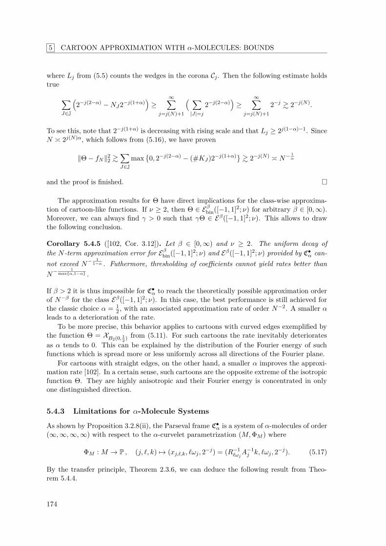
5 CARTOON APPROXIMATION WITH α-MOLECULES: BOUNDS
where Lj from (5.5) counts the wedges in the corona Cj . Then the following estimate holdstrue
J∈J
2−j(2−α) −NJ2−j(1+α)
≥
∞j=j(N)+1
|J |=j
2−j(2−α)
≥∞
j=j(N)+12−j & 2−j(N).
To see this, note that 2−j(1+α) is decreasing with rising scale and that Lj ≥ 2j(1−α)−1. SinceN ≍ 2j(N)α, which follows from (5.16), we have proven
∥Θ − fN ∥22 &
J∈J
max0, 2−j(2−α) − (#KJ)2−j(1+α) & 2−j(N) ≍ N− 1
α
and the proof is finished.
The approximation results for Θ have direct implications for the class-wise approxima-tion of cartoon-like functions. If ν ≥ 2, then Θ ∈ Eβ
bin([−1, 1]2; ν) for arbitrary β ∈ [0,∞).Moreover, we can always find γ > 0 such that γΘ ∈ Eβ([−1, 1]2; ν). This allows to drawthe following conclusion.
Corollary 5.4.5 ([102, Cor. 3.12]). Let β ∈ [0,∞) and ν ≥ 2. The uniform decay ofthe N -term approximation error for Eβ
bin([−1, 1]2; ν) and Eβ([−1, 1]2; ν) provided by C•α can-
not exceed N− 11−α . Futhermore, thresholding of coefficients cannot yield rates better than
N− 1
maxα,1−α .
If β > 2 it is thus impossible for C•α to reach the theoretically possible approximation order
of N−β for the class Eβ([−1, 1]2; ν). In this case, the best performance is still achieved forthe classic choice α = 1
2 , with an associated approximation rate of order N−2. A smaller αleads to a deterioration of the rate.
To be more precise, this behavior applies to cartoons with curved edges exemplified bythe function Θ = XB2(0, 1
2 ) from (5.11). For such cartoons the rate inevitably deterioratesas α tends to 0. This can be explained by the distribution of the Fourier energy of suchfunctions which is spread more or less uniformly across all directions of the Fourier plane.
For cartoons with straight edges, on the other hand, a smaller α improves the approxi-mation rate [102]. In a certain sense, such cartoons are the opposite extreme of the isotropicfunction Θ. They are highly anisotropic and their Fourier energy is concentrated in onlyone distinguished direction.
5.4.3 Limitations for α-Molecule Systems
As shown by Proposition 3.2.8(ii), the Parseval frame C•α is a system of α-molecules of order
(∞,∞,∞,∞) with respect to the α-curvelet parametrization (M,ΦM ) where
ΦM : M → P , (j, ℓ, k) →→ (xj,ℓ,k, ℓωj , 2−j) = (R−1ℓωjA−1
j k, ℓωj , 2−j). (5.17)
By the transfer principle, Theorem 2.3.6, we can deduce the following result from Theo-rem 5.4.4.
174
5.5 Appendix: Bessel Functions
Theorem 5.4.6 ([102, Thm. 5.3]). Let α ∈ [0, 1] and let M•α := mλλ∈Λ be a discrete
frame of α-molecules whose parametrization, for some k > 0, is (α, k)-consistent with theα-curvelet parametrization (5.17). Further, assume that for some γ > γ := maxα, 1−α−1
the order (L,M,N1, N2) of M•α satisfies
L ≥ k(1 + γ), M ≥ 3k2 (1 + γ) + α− 3
2 , N1 ≥ k
2 (1 + γ) + 1 + α
2 , N2 ≥ k(1 + γ).(5.18)
Then the coefficients cλλ∈Λ of each representation Θ =
λ∈Λ cλmλ of the function Θfrom (5.11) with respect to M•
α satisfy cλλ∈Λ /∈ ℓp(Λ) for p < 21+γ .
Proof. Let p < 21+γ and assume that cλλ ∈ ℓp(Λ). According to Theorem 2.3.6 con-
dition (5.18) ensures that the systems M•α and C•
α are sparsity equivalent in ℓp, whichmeans ∥⟨mλ, ψµ⟩λ,µ∥ℓp→ℓp < ∞. (see [59, Def. 5.3]). Hence, by sparsity equivalence,⟨Θ, ψµ⟩µ ∈ ℓp(M). Using Θ =
µ⟨Θ, ψµ⟩ψµ and Lemma 2.3.1, this then implies an
N -term approximation rate of order N−γ , in contradiction to Theorem 5.4.4.
5.5 Appendix: Bessel FunctionsIn this appendix we collect some useful facts about Bessel functions mainly taken from [71]and [51]. We are only interested in Bessel functions Jν of integer and half-integer order inthe range ν ∈ −1
2 , 0,12 , 1, . . .. Bessel functions of this kind occur naturally in the Fourier
analysis of radial functions. For t ∈ R+ the value Jν(t) is conveniently defined by either ofthe two series (see [71] and [51, Appendix B.3])
Jν(t) = t
2ν ∞
k=0
(−1)k
Γ(k + 1)Γ(k + ν + 1) t
22k
= 1√π
t2ν ∞
k=0
(−1)kΓ(k + 12)
Γ(k + ν + 1)t2k
(2k)! , (5.19)
where the Gamma function Γ extends the factorial z! to the complex numbers with Γ(z) =(z−1)!. To verify the equivalence of both representations, it is useful to note that Γ(k+ 1
2) =(2k)!k!4k
√π for k ∈ N0. We explicitly remark, that definition (5.19) is also valid for ν = −1
2 ,although this case is not included in the exposition of [51]. As is obvious from the secondrepresentation, the functions Jν of half-integer order can be expressed in closed form interms of trigonometric functions. For integer orders such closed form representations donot exist.
If f(x) = f0(|x|) is a radial function on Rd, d ∈ N, with a suitable function f0 definedon R+
0 = [0,∞), the Fourier transform of f is given by the formula
f(ξ) = 2π|ξ|(d−2)/2
∞
0f0(r)Jd/2−1(2πr|ξ|)rd/2 dr , ξ ∈ Rd.
Applying this formula to the characteristic function XBd(0,1) of the d-dimensional unit ballBd(0, 1) centered at the origin of Rd yields
(XBd(0,1))∧(ξ) = 2π|ξ|(d−2)/2
1
0Jd/2−1(2π|ξ|r)rd/2 dr =
Jd/2(2π|ξ|)|ξ|d/2 , ξ ∈ Rd. (5.20)
175
5 CARTOON APPROXIMATION WITH α-MOLECULES: BOUNDS
Here, for the integration, we used the second of the following recurrence relations [51,Appendix B.2], which are valid for ν ∈ 1
2N and all t ∈ R+,
t−ν+1Jν(t) = − d
dt
t−ν+1Jν−1(t)
and tνJν−1(t) = d
dt
tνJν(t)
.
The case ν = 12 is not treated in [51], yet it can be easily confirmed by a direct calculation.
By scaling, we can further deduce from (5.20) the following Fourier representation ofthe bivariate function Θ(x) = XB2(0,1)(2x), x ∈ R2, from (5.11),
Θ(ξ) = 14(XB2(0,1))∧(ξ/2) = J1(π|ξ|)
2|ξ|, ξ ∈ R2. (5.21)
Important for our investigation in Section 5.4 is the asymptotic behavior of Jν(r) as r → ∞.We cite the following result from [51, Appendix B.8], which states for ν ∈ 1
2N0 the identity
Jν(r) =
2πr
cos(r − πν
2 − π
4 ) +Rν(r) , r ∈ R+, (5.22)
with a function Rν given on R+ by
Rν(r) = (2π)−1/2rν
Γ(ν + 1/2)ei(r−πν/2−π/4)
∞
0e−rttν+1/2[(1 + it/2)ν−1/2 − 1] dt
t
+ (2π)−1/2rν
Γ(ν + 1/2)e−i(r−πν/2−π/4)
∞
0e−rttν+1/2[(1 − it/2)ν−1/2 − 1] dt
t.
Further, for each ν ∈ 12N0 there is a constant Cν > 0 such that Rν satisfies the estimate
|Rν(r)| ≤ Cνr−3/2 whenever r ≥ 1. (5.23)
The representation (5.22) and the estimate (5.23) play an important role in the proof ofLemma 5.4.1. For completeness, let us finally note that the identity (5.22) especially holdstrue in case ν = −1
2 , with vanishing R− 12
≡ 0. This is a direct consequence of the defini-tion (5.19) and the Taylor series of the cosine.
176
Chapter 6
Cartoon Approximation withα-Molecules: Guarantees
In this chapter, which is a follow-up of Chapter 5, we continue with the investigation ofthe approximation performance of α-molecule systems with respect to cartoon-like data.The model setting is the same, i.e., we still consider the cartoon classes Eβ
bin([−1, 1]2; ν) andEβ([−1, 1]2; ν) specified in Definition 5.2.2. The main results, Theorem 6.0.1 ([60, Thm. 4.1])and Theorem 6.0.2 ([59, Thm. 5.12]) which will be proved below, are approximation guar-antees which nicely complement the bounds established in the previous chapter.
Recall that the order of the N -term approximation rate achievable for the classesEβ
bin([−1, 1]2; ν), ν ≥ 1, and Eβ([−1, 1]2; ν), ν > 0, cannot exceed N−β . This bound, es-tablished in Theorem 5.3.3 (see also Remark 5.3.4), is valid for arbitrary dictionaries andindependent of the approximation scheme employed, as long as a polynomial depth searchcondition is fulfilled. Even adaptive approximation schemes cannot perform better.
Schemes, where these rates are provably achieved, at least up to order, have been de-veloped for binary cartoons based on wedgelets [35] and surflets [19], for general cartoonsutilizing bandelets [86, 87], to give a few examples. These results show that the optimalitybenchmark N−β can indeed be realized in practice, at least up to order. However, theutilized schemes are mostly adaptive, only for certain cartoon classes nonadaptive methodswith quasi-optimal performance are known.
A breakthrough concerning the nonadaptive approximation of cartoon-like functions wasthe introduction of the classic curvelets by Candès and Donoho [14, 15]. By a simple thresh-olding scheme, they achieve an approximation rate for the class E2([−1, 1]2; ν) matching theclass bound N−2 up to a log-factor. The reason for this quasi-optimal performance is theparabolic scaling law employed. The following argument shall heuristically explain, whyparabolic scaling is ideal for the representation of C2 edges.
In local Cartesian coordinates, a C2 curve can be represented as the graph (E(x), x) of afunction E ∈ C2(R) and one can choose a coordinate system such that E′(0) = E(0) = 0. ATaylor expansion then yields approximately E(x) ≈ 1
2E′′(0)x2, which matches the essential
support width ≈ length2 of parabolically scaled functions. Hence, those can provide optimalresolution of the curve across all scales.
The quasi-optimal performance of curvelets for the class Eβ([−1, 1]2; ν) with β = 2 raisedthe question if similar quasi-optimal results can be obtained for other cartoon classes witha regularity β = 2. At least in the range β ∈ (1, 2), a heuristic, similar to the one givenabove for C2 curves, applies to Cβ curves. Generally, if β ∈ (1, 2], a Taylor expansion ofE ∈ Cβ(R) yields |E(x)| . xβ , and thus the boundary curve is contained in a rectangle ofsize width ≈ lengthβ . This suggests α-scaling with α = β−1 for optimal approximation.
And indeed, quasi-optimal approximation could be shown in [73, 83] for α-shearlet
177
6 CARTOON APPROXIMATION WITH α-MOLECULES: GUARANTEES
frames if α = β−1 and β ∈ (1, 2]. For α-curvelets, the classic approximation result byCandès and Donoho was extended in [60, Thm. 4.1]. This extension is stated below, slightlymodified to fit into our model setting, since the class Eβ([−1, 1]2; ν) used here is not fullyidentical to the class used in [60].
Theorem 6.0.1 ([60, Thm. 4.1]). Let β ∈ (1, 2], ν > 0. For the choice α = β−1, theParseval frame of α-curvelets C•
α constructed in Subsection 3.2.3 provides almost optimalsparse approximations for the class of cartoon-like functions Eβ([−1, 1]2; ν). More precisely,there exists a constant C > 0 such that for every f ∈ Eβ([−1, 1]2; ν) and N ∈ N
∥f − fN ∥22 ≤ CN−β log2(1 +N)1+β ,
where fN denotes the N -term approximation of f obtained by choosing the N largest coef-ficients.
When we compare this theorem with the benchmark Theorem 5.3.3, we see that theframe C•
α = ψµµ∈M attains the maximal achievable approximation rate up to a log-factor.Moreover, as for the classical curvelets, this rate is achieved by simply thresholding theframe coefficients, leading to an intrinsically non-adaptive approximation scheme.
Unfortunately, Theorem 5.4.2 proved in the previous chapter shows that α-curvelets arenot able to provide approximation rates beyond N−2, which is suboptimal for Eβ([−1, 1]2; ν)if β > 2. This is due to the fact that α-scaling is not able to take advantage of smoothnessbeyond C2. Further, Theorem 5.4.6 is an indicator that also more general α-moleculesystems are not able to overcome this N−2 barrier. In fact, up to now no frame constructionis known where a nonadaptive thresholding scheme yields approximation rates better thanN−2 for Eβ([−1, 1]2; ν). Therefore further research is required and new ideas need to beconsidered.
Let us now turn to the proof of Theorem 6.0.1. It is based on an analysis of the decayof the curvelet coefficients θµµ∈M given by θµ = ⟨f, ψµ⟩ for a signal f ∈ Eβ([−1, 1]2; ν).This analysis will be conducted below, beginning in Section 6.1, with the main result beingTheorem 6.1.1. It shows that θµµ ∈ ωℓp(M) with p = 2/(1 + β) + ε and ε > 0 arbitrarilysmall. This decay rate is in fact sufficient for a proof of Theorem 6.0.1 via Lemma 2.3.1.
Before turning to Section 6.1, let us state another consequence of Theorem 6.1.1. Byapplying the transfer principle, Theorem 2.3.6, it is possible to deduce approximation ratesfor more general α-molecule systems. Let (M,ΦM ) denote the parametrization (3.28) ofthe Parseval frame of α-curvelets C•
α. Then we can formulate the following theorem, whichis the other main result of this chapter.
Theorem 6.0.2 ([59, Thm. 5.12]). Let β ∈ (1, 2], ν > 0, and α = β−1. Assume that, forsome k > 0, a discrete frame mλλ∈Λ of α-molecules satisfies the following two conditions:
(i) its parametrization (Λ,ΦΛ) and (M,ΦM ) are (α, k)-consistent,
(ii) its order (L,M,N1, N2) satisfies
L ≥ k(1+β), M ≥ 3k2 (1+β)+α− 3
2 , N1 ≥ k
2 (1+β)+1 + α
2 , and N2 ≥ k(1+β).
178
6.1 Sparsity of Curvelet Coefficients
Then each dual frame mλλ∈Λ possesses an almost optimal N -term approximation rate forthe class of cartoon-like functions Eβ([−1, 1]2; ν), i.e., for all f ∈ Eβ([−1, 1]2; ν),
∥f − fN ∥22 . N−β+ε, ε > 0 arbitrary,
where fN denotes the N -term approximation obtained from the N largest frame coefficients.
Note that, by Corollary 3.4.4, the required condition (i) holds in particular for the α-curvelet and α-shearlet parametrizations, for k > 2. Thus, this result allows a simple andsystematic derivation of approximation results for α-curvelets and α-shearlets. For example,we obtain the statement of [59, Thm. 5.13] on cartoon approximation with band-limitedα-shearlet systems, where the optimal approximation rate is reached up to an arbitrarilysmall deviation ε > 0.
6.1 Sparsity of Curvelet Coefficients
The main statements of this chapter, Theorem 6.0.1 and Theorem 6.0.2, are both conse-quences of the following result on the coefficient decay of curvelet coefficients.
Theorem 6.1.1 ([60, Thm. 4.2]). Let θ∗N denote the (in modulus) N th largest curvelet
coefficient. Then there exists some universal constant C such that
supf∈Eβ([−1,1]2;ν)
|θ∗N | ≤ C ·N−(1+β)/2 · (log2N)(1+β)/2 .
This theorem is the centerpiece for proving both Theorem 6.0.1 and Theorem 6.0.2. Infact, Theorem 6.1.1 together with Lemma 2.3.1 directly leads to Theorem 6.0.1.
Proof of Theorem 6.0.1. Applying Lemma 2.3.1 and Theorem 6.1.1 we can estimate
∥f − fN ∥2 .
m>N
|θ∗m|2 .
m>N
m−(1+β) · (log2m)(1+β) . ∞
Nt−(1+β) · (log2 t)
(1+β) dt.
Using partial integration we obtain ∞
Nt−(1+β) · (log2 t)
(1+β) dt . [−t−β (log2 t)(1+β)]∞N +
∞
Nt−(1+β) · (log2 t)
β dt
. N−β (log2N)(1+β) + ∞
Nt−(1+β) · (log2 t)
⌈β⌉ dt
. . . . . N−β (log2N)(1+β) + ∞
Nt−(1+β) dt
. N−β (log2N)(1+β) .
Using the transfer principle, Theorem 2.3.6, it is further possible to deduce Theo-rem 6.0.2.
179
6 CARTOON APPROXIMATION WITH α-MOLECULES: GUARANTEES
Proof of Theorem 6.0.2. Let C•α = ψµµ∈M be the α-curvelet frame from Definition 3.2.6,
and let f ∈ Eβ([−1, 1]2; ν). By Theorem 6.1.1, the sequence of curvelet coefficients θµµ
given by θµ = ⟨f, ψµ⟩ belongs to ωℓp(M) for every p > 21+β . Since ωℓp → ℓp+ε for arbitrary
ε > 0, this further implies θµµ ∈ ℓp(M) for every p > 21+β .
By Theorem 2.3.6, conditions (i) and (ii) guarantee that the frame mλλ∈Λ is sparsityequivalent to ψµµ∈M in ℓp for every p > 2
1+β . This implies that the cross-Gramian⟨ψµ,mλ⟩µ,λ is a bounded operator ℓp(M) → ℓp(Λ). It maps θµµ to the sequence cλλ
given bycλ =
µ
⟨ψµ,mλ⟩θµ = ⟨f,mλ⟩.
As a consequence, cλλ ∈ ℓp(Λ) for every p > 21+β . The embedding ℓp → ωℓp further
proves cλλ ∈ ωℓp(Λ) for every p > 21+β .
Finally observe that we can expand f with respect to the dual frame mλλ in thefollowing way,
f =λ∈Λ
cλmλ.
Hence, for arbitrary ε > 0, an application of Lemma 2.3.1 yields
∥f − fN ∥22 . N−β+ε,
where fN denotes the N -term approximation with respect to the dual frame mλλ obtainedby choosing the N largest coefficients.
It remains to prove Theorem 6.1.1. For this, we first recall the a-priori estimate (5.14)for the size of the curvelet coefficients θµ = ⟨f, ψµ⟩ at scale j, namely
|θµ| = |⟨f, ψµ⟩| ≤ ∥f∥∞∥ψµ∥1 ≤ B∥f∥∞2−(1+α)j/2 (6.1)
with a constant B > 0 independent of the index µ ∈ M .Using this estimate together with Theorem 6.1.2, which is stated and proved below, we
can give a proof of Theorem 6.1.1.
Proof of Theorem 6.1.1. Let Mj ⊂ M denote the indices corresponding to curvelets at scalej, and for ε > 0 put
Mj,ε =µ ∈ Mj , |θµ| > ε
.
By Theorem 6.1.2, which is stated and proved below, we have for ε > 0
#Mj,ε = #µ ∈ Mj , |θµ| > ε
. ε−2/(1+β). (6.2)
On the other hand, (6.1) shows that there is a constant B, independent of scale, such that
|θµ| ≤ B∥f∥∞2−(1+α)j/2.
It follows that for each ε > 0 there is jε such that at scales j ≥ jε the coefficients satisfyθµ < ε. Hence, for j ≥ jε
#Mj,ε = #µ ∈ Mj , |θµ| > ε
= 0.
180
6.1 Sparsity of Curvelet Coefficients
The number of scales at which Mj,ε is nonempty is therefore bounded by
21 + α
log2(B) + log2(∥f∥∞) + log2(ε−1)
. log2(ε−1). (6.3)
It follows from (6.2) and (6.3) that there is a constant C ≥ 1 such that
#µ ∈ M, |θµ| > ε
=
j
#µ ∈ Mj , |θµ| > ε
≤ Cε−2/(1+β) log2(ε−1).
Let θ∗N be the Nth largest coefficient. Then for εN > δN , where δN satisfies N =Cδ−2/(1+β)
N log2(δ−1N ), we have |θ∗
N | ≤ εN . If N ≥ 2 it holds CN4/(1+β) log2(N2) ≥ N ,because 1 ≤ β ≤ 2 and C ≥ 1. For N ≥ 2 therefore
N4/(1+β) log2(N2) ≥ δ−2/(1+β)N log2(δ−1
N ).
This implies δN ≥ N−2, and we can conclude that εN > δN if we choose εN as the solutionof
N = Cε−2/(1+β)N log2(N2).
This choice leads to
εN = (2 C)(1+β)/2 ·N−(1+β)/2(log2N)(1+β)/2,
which proves our claim with constant C = (2 C)(1+β)/2.
The last missing piece is now Theorem 6.1.2.
Theorem 6.1.2 ([60, Thm. 4.3]). Let Mj denote the curvelet indices at scale j. Thesequence θµµ∈Mj obeys
∥θµµ∈Mj ∥wℓ2/(1+β) ≤ C,
for some constant C > 0 independent of scale j.
The proof of this theorem is rather involved. In fact, the remainder of this whole chapteris solely devoted to this task. Thereby, we follow the exposition in [60]. The techniquesused are very similar to those in [15, Sec. 5]. Due to the presence of fractional smoothness,however, some new tools involving divided differences have to be applied.
In a first step, we smoothly decompose f ∈ Eβ([−1, 1]2; ν) into so-called fragments,which can then be analyzed separately. For that we cover R2 at each scale j ∈ N0 withcubes
Q = [(k1 − 1)2−jα, (k1 + 1)2−jα] × [(k2 − 1)2−jα, (k2 + 1)2−jα] , (k1, k2) ∈ Z2,
which we collect in the sets Qj . Further, we put Q :=
j∈N0 Qj . Note how the size of thesquares depends upon the scale 2−j : The ‘width’ of the curvelets at scale j obeys ∼ 2−j
and the ‘length’ of the curvelets is approximately ∼ 2−αj . Thus, the size of the squares isabout the length of the curvelets.
Next, we take a smooth partition of unity ωQQ∈Qj , where these squares are usedas the index set and the functions ωQ are supported in the corresponding squares Q :=(2−jαk1, 2−jαk2) + [−2−jα, 2−jα]2. More precisely, for some fixed nonnegative C∞-function
181
6 CARTOON APPROXIMATION WITH α-MOLECULES: GUARANTEES
ω vanishing outside the square [−1, 1]2, we put ωQ = ω(2jαx1 − k1, 2jαx2 − k2) and assumethat
Q∈Qj
ωQ(x) ≡ 1. The cartoon f = f0 + f1XB ∈ Eβ([−1, 1]2; ν) can then at each scalej ∈ N0 be smoothly localized into the fragments
fQ := fωQ, Q ∈ Qj .
For Q ∈ Qj let θQ denote the curvelet coefficient sequence of fQ at scale j, i.e.,
θQ =
⟨fQ, ψµ⟩
µ∈Mj
. (6.4)
The strategy laid out in [15] is to analyze the sparsity of the sequences θQ and combinethese results to obtain Theorem 6.1.2. In this investigation we have to distinguish betweentwo cases: Either the square Q ∈ Qj meets the edge curve Γ = ∂B of the cartoon or not.Accordingly, we let Q1
j be the subset of Qj containing those cubes, which intersect the edgecurve Γ. Among the remaining cubes of Qj we collect those, which intersect supp f , in Q0
j .The others can be neglected, because they lead to trivial sequences θQ.
The following two propositions ([60, Thm. 4.4] and [60, Thm. 4.5]) directly lead toTheorem 6.1.2.
Theorem 6.1.3 (Analysis of a Smooth Fragment). Let Q be a square such that Q ∈ Q0j .
The curvelet coefficient sequence θQ defined in (6.4) obeys
∥θQ∥wℓ2/(1+β) ≤ C · 2−(1+α)j ,
for some constant C > 0 independent of Q and j.
Theorem 6.1.4 (Analysis of an Edge Fragment). Let Q be a square such that Q ∈ Q1j .
The curvelet coefficient sequence θQ defined in (6.4) obeys
∥θQ∥wℓ2/(1+β) ≤ C · 2−(1+α)j/2,
for some constant C > 0 independent of Q and j.
Theorem 6.1.2 is an easy consequence of these two results and the observation, thatthere are constants A0 and A1, independent of scale, such that
#Q0j ≤ A022αj and #Q1
j ≤ A12αj . (6.5)
The estimates (6.5) hold true since f is supported in [−1, 1]2.
Proof of Theorem 6.1.2. For 0 < p ≤ 1 we have the p-triangle inequality
∥a+ b∥pwℓp ≤ ∥a∥p
wℓp + ∥b∥pwℓp , a, b ∈ wℓp.
Since θµµ∈Mj =
Q∈QjθQ, we can conclude
∥θµµ∈Mj ∥2/(1+β)wℓ2/(1+β) ≤
Q∈Qj
∥θQ∥2/(1+β)wℓ2/(1+β)
≤#Q1
j
· sup
Q1j
∥θQ∥2/(1+β)wℓ2/(1+β) +
#Q0
j
· sup
Q0j
∥θQ∥2/(1+β)wℓ2/(1+β) .
The claim follows now from the above two theorems together with observation (6.5).
182
6.2 Analysis of a Smooth Fragment
It remains to prove Theorems 6.1.3 and 6.1.4. For that let Q ∈ Qj be a fixed cube ata fixed scale j ∈ N0, which nontrivially intersects supp f . We need to analyze the decayof the sequence θQ = ⟨fQ, ψµ⟩µ∈Mj . Since the frame elements ψµ are bandlimited, it isadvantageous to turn to the Fourier side. The Plancherel identity yields
⟨fQ, ψµ⟩ = ⟨ fQ, ψµ⟩.
These scalar products can be estimated, if we have knowledge about the localization of thefunctions fQ. This investigation is carried out separately in Sections 6.2 and 6.3 for thecases Q ∈ Q0
j and Q ∈ Q1j , respectively.
6.2 Analysis of a Smooth Fragment
The goal of this section ([60, Sec. 5]) is a proof of Theorem 6.1.3. Broadly, we follow thearguments in [15, Sec. 8] for β = 2, but with the important difference that our signal classEβ([−1, 1]2; ν) generally involves functions with smoothness of fractional order. This forcesus to translate several estimates in [15] for derivatives of various functions into estimatesfor corresponding moduli of smoothness. The same remark applies to the next Section 6.3.
An important tool is the forward difference operator ∆(h1,h2), where h1, h2 ∈ R, whichacts on a bivariate function f : R2 → R as follows,
∆(h1,h2)f(x1, x2) := f(x1 + h1, x2 + h2) − f(x1, x2). (6.6)
Its one-dimensional analogon takes the simple form ∆hf(t) := f(t + h) − f(t) for h ∈ R.When applied to a bivariate function f : R2 → R, to simplify notation, the operator ∆h
shall exclusively act on variables denoted t or τ ∈ R, e.g., the symbol ∆hf(t, u) denotes thefunction (t, u) →→ f(t+ h, u) − f(t, u). Note that the symbol ∆ without a subscript denotesthe standard Laplacian.
Let us now come back to the proof of Theorem 6.1.3 and recall the notation introducedat the end of the previous section. We treat the case Q ∈ Q0
j , where the cube Q does notintersect the edge curve Γ = ∂B. In this case we call fQ = fωQ a smooth fragment.
Before we begin, we briefly recall our setting. The parameters α ∈ [12 , 1) and β = α−1 ∈
(1, 2] are fixed, as is f ∈ Eβ([−1, 1]2; ν). Since Q does not intersect the edge curve, there isa function g ∈ Cβ(R2) such that fQ = gωQ. By smoothly cutting g off outside the square[−1, 1]2, we can even assume g ∈ Cβ
0 (R2).We want to analyze fQ and for simplicity we look at the following model situation.
Without loss of generality we assume that the cube Q is centered at the origin, by possiblytranslating the coordinate system. In this case the smooth fragment takes the simple form
fj(x) := fQ(x) = g(x)ω(2αjx), x ∈ R2,
where g ∈ Cβ0 (R2) and ω ∈ C∞
0 (R2) with suppω ⊂ [−1, 1]2 is the fixed window generatingthe partition of unity (ωQ)Q (note that by our simplifications the fragment fQ only dependson the scale j and therefore the notation fj is justified).
By rescaling fj we obtain for each scale j the functions
Fj(x) = g(2−αjx)ω(x), x ∈ R2, (6.7)
with suppFj ⊂ [−1, 1]2. We put gj(x) := g(2−αjx), so that we can write Fj(x) = gj(x)ω(x).It is important to note, that gj and Fj depend on the scale, whereas ω remains fixed.
183
6 CARTOON APPROXIMATION WITH α-MOLECULES: GUARANTEES
6.2.1 Fourier Analysis of a Smooth Fragment
We first analyze the localization of Fj , where Fj is given as in (6.7). The key result in thisdirection will be Proposition 6.2.2. Its proof relies on Lemma 6.2.1 below. Here we use theforward difference operator (6.6) defined above.
Lemma 6.2.1. Let α ∈ [12 , 1) and β = α−1 ∈ (1, 2]. Assume that h = C2−(1−α)j for some
fixed constant C > 0, and put N := 2 + ⌈ α1−α⌉. We then have
∥∆N(h,0)∂1Fj∥2
2 . h2β2−2jα,
where the implicit constant is independent of the scale j. Notice that h is not independentand depends on the scale j.
Proof. Since suppFj ⊂ [−1, 1]2 it suffices to prove
∥∆N(h,0)∂1Fj∥∞ . hβ2−jα. (6.8)
By the product rule we have ∂1Fj = ∂1gj · ω + gj · ∂1ω and it holds
∆N(h,0)
∂1gj · ω
=
Nk=0
∆k(h,0)∂1gj · ∆N−k
(h,0)ω(· + kh, ·),
∆N(h,0)
gj · ∂1ω
=
Nk=0
∆k(h,0)gj · ∆N−k
(h,0)∂1ω(· + kh, ·).(6.9)
Clearly, we have ∥∂1gj∥∞ . 2−αj and for every k ∈ N0 the estimates ∥∆k(h,0)ω∥∞ . hk and
∥∆k(h,0)∂1ω∥∞ . hk. According to Lemma 6.4.3, it further holds
∥∆(h,0)gj∥∞ . h2−αj and ∥∆k(h,0)gj∥∞ . hβ2−j for k ≥ 2,
as well as ∥∆k(h,0)∂1gj∥∞ . hβ2−αj for k ≥ 1.
Since N ≥ 3, these estimates suffice to bound the summands in (6.9) for k = 0. In casek = 0, we observe that hN . hβ2−jα, due to N ≥ β + α
1−α . The assertion (6.8) follows.
The previous lemma is key to the proof of the following proposition. Here we use thenotation |ξ| ∼ 2(1−α)j to indicate |ξ| ∈ [C12(1−α)j , C22(1−α)j ] for some arbitrary but fixedconstants 0 < C1 ≤ C2 < ∞. A typical choice would be C1 = 1 and C2 = 21−α.
Proposition 6.2.2 ([60, Prop. 5.2]). It holds independently of the scale j|ξ|∼2(1−α)j
| Fj(ξ)|2 dξ . 2−2βj .
Proof. Let 0 < C1 ≤ C2 < ∞ be fixed and choose C > 0 such that C2C < 2π. Puttingh := C2−(1−α)j , there then exists c > 0 such that |eiξ1h − 1|2 ≥ c for every ξ1 with|ξ1| ∈ [C12(1−α)j , C22(1−α)j ]. Using Lemma 6.2.1 with N := 2 + ⌈ α
1−α⌉ we then estimate the
184
6.2 Analysis of a Smooth Fragment
integrals on the vertical strips:
22(1−α)j
|ξ1|∼2(1−α)j
ξ2
| Fj(ξ1, ξ2)|2 dξ2 dξ1 ≍
|ξ1|∼2(1−α)j
ξ2
|ξ1|2| Fj(ξ1, ξ2)|2 dξ2 dξ1
.
|ξ1|∼2(1−α)j
ξ2
|eiξ1h − 1|2N |ξ1|2| Fj(ξ1, ξ2)|2 dξ2 dξ1
=
|ξ1|∼2(1−α)j
ξ2
| ∆N(h,0)∂1Fj(ξ1, ξ2)|2 dξ2 dξ1
≤R2
| ∆N(h,0)∂1Fj(ξ)|2 dξ = ∥∆N
(h,0)∂1Fj∥22 . h2β2−2jα.
Interchanging ξ1 and ξ2 yields analogous estimates for the horizontal strips. Altogether, weobtain
|ξ|∼2(1−α)j| Fj(ξ)|2 dξ . 2−2j(1−α)h2β2−2jα ≍ 2−2βj .
As an immediate conclusion, we deduce a corresponding estimate for the original smoothfragment fj .
Theorem 6.2.3 ([60, Thm. 5.3]). We have independently of scale j|ξ|∼2j
| fj(ξ)|2 dξ . 2−2(β+α)j .
Proof. The statement follows from the relation fj(ξ) = 2−2αj Fj(2−αjξ).
Finally, we state a refinement of Theorem 6.2.3.
Corollary 6.2.4 ([60, Cor. 5.4]). Let m = (m1,m2) ∈ N20 and ∂m = ∂m1
1 ∂m22 . We have
|ξ|∼2j|∂m fj(ξ)|2 dξ . 2−2jα|m|12−2(β+α)j .
Proof. Recall that fj = gω(2αj ·). Let us define the window ω(x) := xmω(x) and thefunction fj(x) := g(x)ω(2αjx) for x ∈ R2. Then because of ω(2αjx) = 2jα|m|1xmω(2αjx) forevery x ∈ R2
xmfj(x) = g(x)xmω(2αjx) = 2−jα|m|1g(x)ω(2αjx) = 2−jα|m|1 fj(x).
We conclude with Theorem 6.2.3|ξ|∼2j
|∂m fj(ξ)|2 dξ =
|ξ|∼2j| xmfj(x)(ξ)|2 dξ
= 2−2jα|m|1
|ξ|∼2j|F fj(ξ)|2 dξ . 2−2jα|m|12−2(β+α)j .
185
6 CARTOON APPROXIMATION WITH α-MOLECULES: GUARANTEES
6.2.2 Curvelet Analysis of a Smooth Fragment
Let J = (j, ℓ) be a scale-angle pair and WJ the wedge function from (5.6), used in theconstruction of the α-curvelet frame C•
α. Then WJ is a non-negative real-valued function,supported in the wedge pair W+
J given in (5.9) and satisfying ∥WJ∥∞ ≤ 1.Theorem 6.2.3 directly leads to a central result, namely that it holds
R2
|J |=j
|( fjWJ)(ξ)|2 dξ . 2−2j(β+α). (6.10)
Recall the notation |J | = j. Our next goal, is to refine this result. Let us first record abasic fact.
Lemma 6.2.5 ([60, Lem. 5.5]). Let m ∈ N20. It holds for all ξ ∈ R2
|J |=j
|∂mWJ(ξ)|2 . 2−2jα|m|1 .
Proof. From the definition it follows that WJ scales with 2−αj in one direction and with2−j in the orthogonal direction. No matter what direction, we always do better than|∂mWJ(ξ)|2 . 2−2jα|m|1 . For fixed ξ only a fixed number of summands are not zero, uni-formly for all ξ. The claim follows.
Next we prove an auxiliary lemma. Here ∆ = ∂21 + ∂2
2 denotes the standard Laplacian.
Lemma 6.2.6 ([60, Lem. 5.6]). Let ∆ = ∂21 + ∂2
2 denote the standard Laplacian. It holdsfor m ∈ N0
R2
|J |=j
|∆m( fjWJ)(ξ)|2 dξ . 2−2j(β+α) · 2−4mαj .
Proof. For m = 0 this is just (6.10), a direct consequence of Theorem 6.2.3. Now let m > 0.It holds with a, b ∈ N2
0 and certain coefficients ca,b ∈ N0
∆m( fjWJ)(ξ) =
|a|+|b|=2m
ca,b∂a fj(ξ)∂bWJ(ξ).
Let a, b ∈ N20 such that |a|1 + |b|1 = 2m. Then with Lemma 6.2.5 and Corollary 6.2.4
R2
|J |=j
|∂a fj(ξ)|2|∂bWJ(ξ)|2 dξ . 2−2jα|b|1
|ξ|∼2j|∂a fj(ξ)|2 dξ
. 2−2jα|b|12−2jα|a|12−2(β+α)j
= 2−2jα(|a|1+|b|1)2−2(β+α)j = 2−4jαm2−2(β+α)j .
Now we come to the refinement of (6.10). For that, we need the differential operator
L = I − 22αj∆, (6.11)
where I is the identity and ∆ the standard Laplacian. The theorem below shows thatL2( fjWJ) obeys the same estimate (6.10) as fjWJ .
186
6.2 Analysis of a Smooth Fragment
Theorem 6.2.7 ([60, Thm. 5.7]). Let L be the differential operator defined in (6.11). Itholds
R2
|J |=j
|L2( fjWJ)(ξ)|2 dξ . 2−2j(β+α).
Proof. It holdsL2 = I − 2 · 22αj∆ + 24αj∆2.
Applying (6.10) and Lemma 6.2.6 yields the desired result.
Finally we can give the proof of Theorem 6.1.3.
6.2.3 Proof of Theorem 6.1.3
Proof. Recall the curvelet frame C•α = ψµµ∈M . On the Fourier side
ψj,ℓ,k = WJuj,k(RJ ·),
with rotation matrix RJ given as in (3.24) and functions
uj,k(ξ) := 2−j(1+α)/2e2πi(2−jk1,2−αjk2)·ξ, ξ ∈ R2.
We have to study the decay of the sequence θQ defined in (6.4). Its elements θj,ℓ,k :=⟨fj , ψj,ℓ,k⟩ are given by the formula
θj,ℓ,k =R2fjWJ(ξ)uj,k(RJξ) dξ.
We observe
Luj,k = (1 + 2−2j(1−α)k21 + k2
2)uj,k,
which also holds for the rotated versions uj,k(RJ ·). Partial integration thus yields
θj,ℓ,k =R2fj(ξ)WJ(ξ)uj,k(RJξ) dξ = (1 + 2−2j(1−α)k2
1 + k22)−2
R2
L2( fjWJ)uj,k(RJξ) dξ.
For j ∈ N and K = (K1,K2) ∈ Z2 we define the set
Zj,K :=
(k1, k2) ∈ Z2 : k12−j(1−α) ∈ [K1,K1 + 1), k2 = K2.
Further, we putMj,K :=
µ = (j, ℓ, k) ∈ Mj : k ∈ Zj,K
,
where Mj denotes the curvelet indices at scale j. It follows from the orthogonality propertiesof the Fourier system uj,kk∈Z2 that
k∈Zj,K
|θj,ℓ,k|2 ≤ (1 + |K|22)−4R2
|L2( fjWJ)(ξ)|2 dξ,
187
6 CARTOON APPROXIMATION WITH α-MOLECULES: GUARANTEES
where |K|22 = K21 +K2
2 . We further concludeµ∈Mj,K
|θµ|2 =
|J |=j
k∈Zj,K
|θJ,k|2 ≤ (1 + |K|22)−4R2
|J |=j
|L2( fjWJ)(ξ)|2 dξ.
Now we apply Theorem 6.2.7 and obtainµ∈Mj,K
|θµ|2 . 2−2j(β+α)(1 + |K|22)−4,
which directly implies θµµ∈Mj,K
ℓ2 . 2−j(β+α)(1 + |K|22)−2. (6.12)
It holds #Zj,K ≤ 1 + 2j(1−α) and therefore, since Lj = 2⌊j(1−α)⌋, the estimate #Mj,K ≤2 · 22j(1−α). Now we recall the interpolation inequality ∥cλλ∥ℓp ≤ n1/p−1/2∥cλλ∥ℓ2 for afinite sequence cλλ with n nonzero entries. Applying this inequality with p = 2/(1 + β)and n = 2 · 22j(1−α) the maximal size of Mj,K , we get from (6.12)θµµ∈Mj,K
ℓ2/(1+β) . 2j(β−1)θµµ∈Mj,K
ℓ2 ≤ 2−j(1+α)(1 + |K|22)−2.
It followsµ∈Mj,K
|θµ|2/(1+β) . 2−j(1+α)2/(1+β) · (1 + |K|22)−4/(1+β) = 2−2αj(1 + |K|22)−4/(1+β).
Finally, we haveµ∈Mj
|θµ|2/(1+β) =
K∈Z2
µ∈Mj,K
|θµ|2/(1+β) ≤ 2−2αj
K∈Z2
(1 + |K|22)−4/(1+β) . 2−2αj .
The desired estimate for the sequence θQ = θµµ∈Mj follows, i.e.,
∥θQ∥ℓ2/(1+β) . 2−j(α+1).
The following section is devoted to the proof of Theorem 6.1.4.
6.3 Analysis of an Edge Fragment
Let us turn to the more complicated case Q ∈ Q1j and the proof of Theorem 6.1.4. In this
case the cube Q intersects the edge curve Γ and fQ = fωQ is accordingly called an edgefragment. The subsequent exposition is taken from [60, Sec. 6].
Again we follow the broad outline for the case β = 2 which has been established in [15],and again we will need to adapt the estimates of [15, Sec. 6] to functions of fractional ordersmoothness via the use of moduli of smoothness. This turns out to cause serious difficultiesand forces us to turn to techniques based on the forward difference operator (6.6).
In order to prove Theorem 6.1.4 we need to analyze the decay of the sequence θQ =⟨fQ, ψµ⟩µ∈Mj = ⟨ fQ, ψµ⟩µ∈Mj . To estimate these scalar products, we again study the
188
6.3 Analysis of an Edge Fragment
localization of the function fQ. As in the treatment of the smooth fragments, our investi-gation starts with some simplifying reductions.
First, we note that it suffices to prove Theorem 6.1.4 for an edge fragment fQ = fωQ,where f ∈ Eβ([−1, 1]2; ν) is a cartoon of the simple form f = gXB with g ∈ Cβ
0 (R2). Infact, the curvelet coefficient sequence of a general edge fragment fQ = f0ωQ + f1XBωQ =:f0
Q + f1Q can be decomposed into θ(0)
Q = ⟨f0Q, ψµ⟩µ∈Mj and θ
(1)Q = ⟨f1
Q, ψµ⟩µ∈Mj . FromTheorem 6.1.3 we already know
∥θ(0)Q ∥wℓ2/(1+β) . 2−(1+α)j . 2−(1+α)j/2 .
Therefore it only remains to show ∥θ(1)Q ∥wℓ2/(1+β) . 2−(1+α)j/2. Since B ⊂ [−1, 1]2, we can
further smoothly cut off f1 ∈ Cβ(R2) outside of [−1, 1]2 to obtain a function g ∈ Cβ0 (R2)
such that f1Q = gXBωQ.
Second, without loss of generality we restrict ourselves to the following model situation.The cube Q is centered at the origin and the edge curve Γ is the graph of a functionE : [−2−jα, 2−jα] → [−2−jα, 2−jα] belonging to Cβ(R), with x1 = E(x2). Further, it shallhold E(0) = E′(0) = 0, so that Γ approximates a vertical line through the origin. If thescale j is big enough, say bigger than some fixed base scale j0 ∈ N0, it is always possible toarrive at this setting by possibly translating or rotating the coordinate axes. Henceforth,we assume j ∈ N and j ≥ j0 which clearly poses no loss of generality.
In this simplified model situation the edge fragment fQ can be written in the form
fj(x) := fQ(x) = ω(2αjx)g(x)Xx1≥E(x2), x = (x1, x2) ∈ R2, (6.13)
where g ∈ Cβ0 (R2), and ω ∈ C∞
0 (R2) is the nonnegative window with suppω ⊂ [−1, 1]2,generating the partition of unity ωQQ.
As in the discussion of the smooth fragments in the previous section, we introduce thenotation fj := fQ for the standard edge fragment (6.13) to indicate the sole dependence onthe scale j. In addition, it is again more convenient to work with rescaled versions Fj ofthe edge fragments fj . Therefore, we put gj := g(2−αj ·) and define
Fj(x) := ω(x)gj(x)Xx1≥Ej(x2), x = (x1, x2) ∈ R2, (6.14)
with the rescaled edge functions
Ej : [−1, 1] → [−1, 1] , Ej(x2) := 2αjE(2−αjx2).
It holds Ej ∈ Cβ([−1, 1]) with E′j = E′(2−αj ·) and Höl(E′
j , β − 1) ≤ δj , where
δj := 2−j(1−α) · Höl(E′, β − 1).
Observe that Höl(E′, β−1) is a constant independent of the scale j. Together with Ej(0) =E′
j(0) = 0 this implies for all u ∈ [−1, 1] that
|Ej(u)| ≤ δj and |E′j(u)| ≤ δj . (6.15)
For convenience, we continuously extend the function Ej to the whole of R by attachingstraight lines on the left and on the right, with constant slopes E′
j(1) and E′j(−1) respec-
tively. Since this extension occurs outside of the square [−1, 1]2, it does not change therepresentation (6.14) of the edge fragment. Furthermore, it also does not alter the regular-ity and the Hölder constant.
189
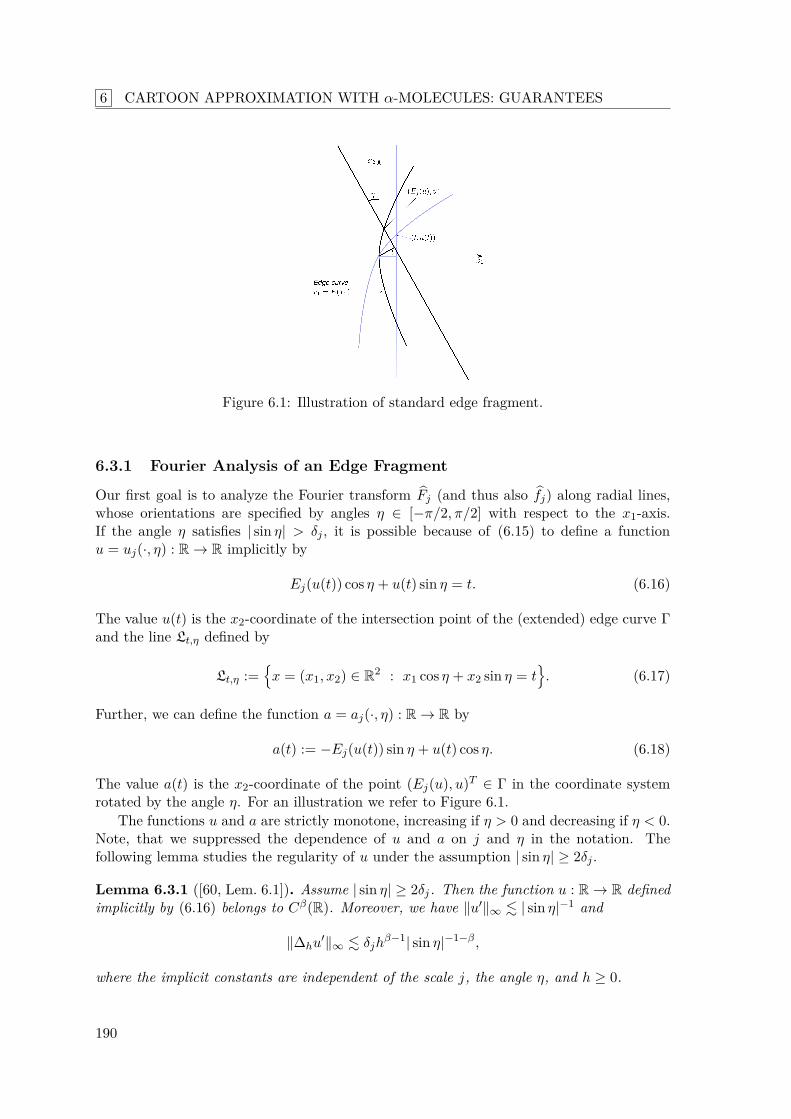
6 CARTOON APPROXIMATION WITH α-MOLECULES: GUARANTEES
Figure 6.1: Illustration of standard edge fragment.
6.3.1 Fourier Analysis of an Edge Fragment
Our first goal is to analyze the Fourier transform Fj (and thus also fj) along radial lines,whose orientations are specified by angles η ∈ [−π/2, π/2] with respect to the x1-axis.If the angle η satisfies | sin η| > δj , it is possible because of (6.15) to define a functionu = uj(·, η) : R → R implicitly by
Ej(u(t)) cos η + u(t) sin η = t. (6.16)
The value u(t) is the x2-coordinate of the intersection point of the (extended) edge curve Γand the line Lt,η defined by
Lt,η :=x = (x1, x2) ∈ R2 : x1 cos η + x2 sin η = t
. (6.17)
Further, we can define the function a = aj(·, η) : R → R by
a(t) := −Ej(u(t)) sin η + u(t) cos η. (6.18)
The value a(t) is the x2-coordinate of the point (Ej(u), u)T ∈ Γ in the coordinate systemrotated by the angle η. For an illustration we refer to Figure 6.1.
The functions u and a are strictly monotone, increasing if η > 0 and decreasing if η < 0.Note, that we suppressed the dependence of u and a on j and η in the notation. Thefollowing lemma studies the regularity of u under the assumption | sin η| ≥ 2δj .
Lemma 6.3.1 ([60, Lem. 6.1]). Assume | sin η| ≥ 2δj. Then the function u : R → R definedimplicitly by (6.16) belongs to Cβ(R). Moreover, we have ∥u′∥∞ . | sin η|−1 and
∥∆hu′∥∞ . δjh
β−1| sin η|−1−β ,
where the implicit constants are independent of the scale j, the angle η, and h ≥ 0.
190
6.3 Analysis of an Edge Fragment
Proof. First of all it is not difficult to show that u = uj(·, η) ∈ C1(R) with
u′(t) =
sin η + E′j(u(t)) cos η
−1.
Under the assumption | sin η| ≥ 2δj it follows ∥u′∥∞ . | sin η|−1 because of |E′j(u)| ≤ δj ≤
12 | sin η| for all u ∈ [−1, 1]. Finally, we examine ∆hu
′. For t ∈ R
∆hu′(t) = u′(t+ h) − u′(t) = u′(t+ h)u′(t)
u′(t)−1 − u′(t+ h)−1
= u′(t+ h)u′(t) cos ηE′
j(u(t)) − E′j(u(t+ h))
.
Using Höl(E′j , β − 1) ≤ δj and the mean value theorem leads to
∥∆hu′∥∞ ≤ ∥u′∥2
∞δj∥∆hu∥β−1∞ ≤ ∥u′∥β+1
∞ δjhβ−1 . δjh
β−1| sin η|−1−β .
The following lemma collects some properties of the function a : R → R defined in(6.18).
Lemma 6.3.2 ([60, Lem. 6.2]). Assume | sin η| ≥ 2δj. It holds a ∈ Cβ(R) with
∥a′∥∞ . | sin η|−1, ∥∆ha∥∞ . h| sin η|−1, ∥∆ha′∥∞ . δjh
β−1| sin η|−1−β ,
with implicit constants independent of j, η, and h ≥ 0.
Proof. This is an easy consequence of the properties of u proved in the previous lemma.
Next, we introduce the scale-dependent interval
I(η) := Ij(η) := [aj(η), bj(η)],
where aj(η) = Ej(−1) cos η − sin η and bj(η) = Ej(1) cos η + sin η. The restrictions of uand a to I(η) correspond precisely to that part of the edge curve Γ lying inside the square[−1, 1]2. In particular, we have a bijection u : I(η) → [−1, 1]. In the sequel it is moreconvenient to work with an extension of I(η), given by
I(η) := Ij(η) := [aj(η) − Cδj , bj(η) + Cδj ], (6.19)
for some suitable fixed constant C > 0.
Lemma 6.3.3 ([60, Lem. 6.3]). For | sin η| > δj we have
|I(η)| . | sin η| and |I(η)| . | sin η|.
Proof. In view of | sin η| > δj and (6.15) we can estimate
|I(η)| ≤ |Ej(1) − Ej(−1)|| cos η| + 2| sin η| ≤ 2δj + 2| sin η| . | sin η|.
The estimate for I(η) then follows directly from | sin η| > δj .
191
6 CARTOON APPROXIMATION WITH α-MOLECULES: GUARANTEES
We want to analyze Fj along lines through the origin with orientation η ∈ [−π/2, π/2].The central tool in this investigation is the Fourier slice theorem. In view of this theorem itmakes sense to first study the Radon transform RFj (see (1.5) for a definition), in particularits regularity. By Paley-Wiener type arguments we can then later extract informationabout the decay of Fj . Basically, this is the same approach taken in [15]. Due to the lack ofregularity in our case, however, we have to use a more refined technique in this investigation.The main idea is to use finite differences instead of derivatives.
The value RFj(t, η) of the Radon transform is obtained by integrating Fj along the lineLt,η defined in (6.17). Rotating Fj by the angle η yields the function F η
j and we can write
(RFj)(t, η) =RF η
j (t, u) du.
The rescaled edge fragment Fj can be rewritten as the product Fj = GjXx1≥Ej(x2) withthe function
Gj := ωg(2−αj ·) = ωgj . (6.20)
Then we have
(RFj)(t, η) = a(t,η)
−∞Gη
j (t, u) du, (6.21)
where Gηj is the function obtained by rotating Gj by the angle η. Using the notation gη
j
and ωη for the rotated versions of gj and ω, the integrand of (6.21) takes the form
Gηj = gη
jωη. (6.22)
We see, that the component gηj = gη(2−αj ·) ∈ Cβ
0 (R2) of Gηj is scaled and the window
ωη ∈ C∞0 (R2) remains fixed.
The central lemma of this subsection is given below. Its proof relies on estimates of thefunctions gη
j and ωη and is outsourced to Section 6.4.
Lemma 6.3.4 ([60, Lem. 6.4]). Assume that | sin η| ≥ 2δj. For h = C2−(1−α)j, whereC > 0 is some fixed constant, we then have
∆h∂1RFj(t, η) = S1,j(t, η) + S2,j(t, η)
with functions S1,j , S2,j such that
∥S1,j(·, η)∥22 . δ2
jh2(β−1)| sin η|−1−2β ,
∥∆(h,0)S2,j(·, η)∥22 . h2β | sin η|−1−2β ,
where the implicit constants are independent of the scale j and the angle η.
The previous lemma is the key to the following proposition. The notation |λ| ∼ 2(1−α)j
indicates that |λ| ∈ [C12(1−α)j , C22(1−α)j ] for fixed constants 0 < C1 ≤ C2 < ∞. A typicalchoice would be C1 = 1 and C2 = 21−α.
192
6.3 Analysis of an Edge Fragment
Proposition 6.3.5 ([60, Prop. 6.5]). It holds|λ|∼2(1−α)j
| Fj(λ cos η, λ sin η)|2 dλ . 2−(1−α)j1 + 2(1−α)j | sin η|
−1−2β
with an implicit constant independent of j and η.
Proof. First we assume | sin η| ≥ 2δj . The integration domain is [C12(1−α)j , C22(1−α)j ] forfixed constants 0 < C1 ≤ C2 < ∞. Let us fix h := C2−j(1−α), where C > 0 is chosensuch that C2C < 2π. For this choice of h there is c > 0 such that |eiλh − 1|2 ≥ c forall |λ| ∈ [C12(1−α)j , C22(1−α)j ] at all scales. We conclude, where S1,j and S2,j denote theentities from Lemma 6.3.4:
|λ|∼2j(1−α)
|λ|2| Fj(λ cos η, λ sin η)|2 dλ .
|λ|∼2j(1−α)
|eiλh − 1|2|λ|2| Fj(λ cos η, λ sin η)|2 dλ
=
|λ|∼2j(1−α)
|F∆h∂1RFj(·, η)
(λ)|2 dλ
.
|λ|∼2j(1−α)
| S1,j(·, η)(λ)|2 dλ+
|λ|∼2j(1−α)
| S2,j(·, η)(λ)|2 dλ
.
|λ|∼2j(1−α)
| S1,j(·, η)(λ)|2 dλ+
|λ|∼2j(1−α)
|eiλh − 1|2| S2,j(·, η)(λ)|2 dλ
≤R
| S1,j(·, η)(λ)|2 dλ+R
|eiλh − 1|2| S2,j(·, η)(λ)|2 dλ
= ∥S1,j(·, η)∥22 + ∥∆hS2,j(·, η)∥2
2 . h2β | sin η|−1−2β .
It follows |λ|∼2j(1−α)
| Fj(λ cos η, λ sin η)|2 dλ . 2−j(1−α)2j(1−α)| sin η|−1−2β
.
Next, we handle the case | sin η| < 2δj . We want to show|λ|∼2j(1−α)
| Fj(λ cos η, λ sin η)|2 dλ . 2−j(1−α). (6.23)
Altogether we then obtain the desired estimate|λ|∼2(1−α)j
| Fj(λ cos η, λ sin η)|2 dλ . 2−(1−α)j1 + 2(1−α)j | sin η|
−1−2β,
since 2(1−α)j | sin η| & 1 if | sin η| ≥ 2δj and 2(1−α)j | sin η| . 1 if | sin η| < 2δj .It remains to show (6.23). For this we write the edge fragment as a sum Fj = F 0
j + F 1j ,
where
F 0j (x) = g(2−jαx)ω(x)Xx1≥δj, x ∈ R2, (6.24)
is a fragment with a straight edge and F 1j (x) = Fj(x) − F 0
j (x) is the deviation.
193
6 CARTOON APPROXIMATION WITH α-MOLECULES: GUARANTEES
The function F 1j is supported in a vertical strip around the x2-axis of width 2δj . For η
satisfying | sin η| < 2δj the Radon transform RF 1j (·, η) is L∞-bounded and supported in an
interval of length
2(δj cos η + sin η) . δj .
It follows ∥RF 1j (·, η)∥2
2 . δj . 2−j(1−α), and therefore|λ|∼2j(1−α)
|F 1j (λ cos η, λ sin η)|2 dλ ≤
R
| RF 1j (·, η)(λ)|2 dλ . 2−j(1−α).
Finally, the estimate |λ|∼2j(1−α)
|F 0j (λ cos η, λ sin η)|2 dλ . 2−j(1−α)
follows from the fact, that we have decay |F 0j (λ, 0)| ∼ |λ|−1/2 normal to the straight singu-
larity curve, and that the second argument (λ sin η) remains bounded due to the condition| sin η| < 2δj . This finishes the proof.
A direct consequence is the following theorem.
Theorem 6.3.6 ([60, Thm. 6.6]). We have|λ|∼2j
| fj(λ cos η, λ sin η)|2 dλ . 2−(1+2α)j1 + 2(1−α)j | sin η|
−1−2β.
Proof. The statement follows directly from the relation fj(ξ) = 2−2αjFj(2−αjξ).
A refinement of the discussion in this subsection, which can be found in Section 6.5,yields the following theorem.
Theorem 6.3.7 ([60, Thm. 6.7]). We have for m = (m1,m2) ∈ N20 the estimate
|λ|∼2j
|∂m fj(λ cos η, λ sin η)|2 dλ
. 2−j2α|m|12−j2(1−α)m12−(1+2α)j
1 + 2(1−α)j | sin η|
−1−2β+ 2(−1−2β)j
.
6.3.2 Curvelet Analysis of an Edge Fragment
In the following J = (j, ℓ) shall denote a scale-angle pair with j ∈ N0, ℓ ∈ 0, . . . , Lj − 1,and WJ shall be the wedge functions from (5.6). Recall also the characteristic angle ωj =π2−⌊j(1−α)⌋ at scale j and the corresponding orientations ωJ := ℓωj , ranging between 0 andπ. From Theorem 6.3.6 we can directly conclude the following result.
Theorem 6.3.8 ([60, Thm. 6.8]). We haveR2
| fjWJ(ξ)|2 dξ . 2−(1+α)j1 + 2(1−α)j | sinωJ |
−1−2β. (6.25)
194
6.3 Analysis of an Edge Fragment
Proof. It holds ∥WJ∥∞ ≤ 1 and suppWJ ⊂ W+J , where W+
J is the wedge defined in (5.9).Let us define the intervals Kj = 1
6π [2j−1, 2j+1] and AJ = [ωJ − 3ωj/4, ωJ + 3ωj/4]. UsingTheorem 6.3.6 we calculate
R2| fjWJ(ξ)|2 dξ ≤
W+
J
| fj(ξ)|2 dξ
=
Kj
AJ
+
π+AJ
| fj(λ, η)|2λ dη dλ
.
AJ
+
π+AJ
2−(1+2α)j
1 + 2(1−α)j | sin η|
−1−2β2j dη
. 2−(1+α)j1 + 2(1−α)j | sinωJ |
−1−2β.
For a scale-angle pair J = (j, ℓ) let us define the quantity
ℓJ = 1 + 2(1−α)j | sinωJ | (6.26)
and the differential operator
L = (I − (2j/ℓJ)2D21)(I − 22αjD2
2) = I − 22jℓ−2J D2
1 − 22αjD22 + 22(1+α)jℓ−2
J D21D2
2, (6.27)
with identity I and partial derivatives
D1 = cosωJ · ∂1 + sinωJ · ∂2 and D2 = − sinωJ · ∂1 + cosωJ · ∂2. (6.28)
We will show that L( fjWJ) obeys the same estimate (6.25) as fjWJ . The key result forthis statement is Theorem 6.3.7
Theorem 6.3.9 ([60, Thm. 6.9]). Let L be the differential operator defined in (6.27). Wehave
R2|L( fjWJ)(ξ)|2 dξ . 2−(1+α)j
1 + 2(1−α)j | sinωJ |
−1−2β.
Proof. First, observe that for each pair m = (m1,m2) ∈ N20 the mixed derivative of WJ
obeys
∥Dm11 Dm2
2 WJ∥∞ = O2−jm1 · 2−jαm2
. (6.29)
This follows from the fact, that the functions WJ from (5.6) scale with their support wedgesW+
J , which are of length ∼ 2j and width ∼ 2αj .Next, from the definition (6.28) of the operators D1 and D2 we deduce for m1 ∈ N0
Dm11fj =
a+b=m1
ca,b(cosωJ)a(sinωJ)b∂(a,b) fj
with binomial coefficients ca,b ∈ N. A similar formula holds for Dm22fj and m2 ∈ N0. Using
| sinωJ | ≤ 2−(1−α)jℓJ with the quantity ℓJ from (6.26) we obtain the estimate
∥Dm11fj∥2
L2(W+J ) .
a+b=m1
| sinωJ |2b · ∥∂(a,b) fj∥2L2(W+
J )
≤
a+b=m1
(2−(1−α)jℓJ)2b · ∥∂(a,b) fj∥2L2(W+
J ).
195
6 CARTOON APPROXIMATION WITH α-MOLECULES: GUARANTEES
Analogously, we obtain
∥Dm22fj∥2
L2(W+J ) .
a+b=m2
∥∂(a,b) fj∥2L2(W+
J ).
Taking into account the width ∼ 2αj of the wedges W+J , Theorem 6.3.7 gives for (a, b) ∈
N20 the bound
∥∂(a,b) fj∥2L2(W+
J ) ≤ Ca,b2αj · 2−j2α(a+b)2−2j(1−α)a2−(1+2α)jℓ−1−2βJ + 2(−1−2β)j,
with some constant Ca,b > 0 independent of scale. Therefore we can estimate for m1 ∈ N0
∥Dm11fj∥2
L2(W+J ) . 2−j2αm1
2−2j(1−α)m12−(1+α)jℓ2m1−1−2β
J + 2αj2(−1−2β)j.If m1 ≤ 2 this further simplifies to
∥Dm11fj∥2
L2(W+J ) . 2−2jm12−(1+α)jℓ2m1−1−2β
J , (6.30)
since for every m1 ≤ (1 + α)/α we have
2αj2(−1−2β)j . 2−2j(1−α)m12−(1+α)jℓ2m1−1−2βJ .
Similar calculations lead to
∥Dm22fj∥2
L2(W+J ) . 2−2αjm22−(1+α)jℓ−1−2β
J . (6.31)
Indeed, if a+ b = m2 we have
∥∂a1∂
b2fj∥2
L2(W+J ) ≤ Ca,b · 2αj · 2−2αjm2
2−(1+2α)jℓ−1−2β
J + 2(−1−2β)j.Since 1 ≤ ℓJ ≤ 2 · 2(1−α)j it holds
2j(1+α)2−2βj = 2−(1−α)(1+2β)j . ℓ−1−2βJ .
Therefore, taking into account 1 ≤ 2(1−α)j , we can conclude
2(−1−2β)j ≤ 2j(1+α)2−2βj2−(1+2α)j . 2−(1+2α)jℓ−1−2βJ .
Altogether we obtain the desired estimate (6.31).After this preliminary work we can finally prove the statement of Theorem 6.3.9. We
have
L( fjWJ) = fjWJ − 22jℓ−2J D2
1( fjWJ) − 22αjD22( fjWJ) + 22(1+α)jℓ−2
J D21D2
2( fjWJ),
which allows us to show the desired estimate for each term separately. For fjWJ the estimateholds true by Theorem 6.3.8.
Let us turn to the second term. The product rule yields
D21( fjWJ) = (D2
1fj)WJ + 2(D1 fj)(D1WJ) + fj(D2
1WJ).
196
6.3 Analysis of an Edge Fragment
The previous estimates together with the Hölder inequality then lead to
∥D21( fjWJ)∥2
2 . 2−4jℓ4J2−(1+α)jℓ−1−2βJ .
Here (6.30) was used, and that ∥Dm11 WJ∥2
∞ ≤ 2−2jm1 ≤ 2−2jm1ℓ2m1J by (6.29). This settles
the claim for the second term.Analogously, we can deduce
∥D22( fjWJ)∥2
2 . 2−4αj2−(1+α)jℓ−1−2βJ ,
using (6.31) and that ∥Dm22 WJ∥2
∞ ≤ 2−2αjm2 by (6.29). This gives the estimate for thethird term.
Finally, it also holds
∥D21D2
2( fjWJ)∥22 . 2−4j(1+α)ℓ4J2−(1+α)jℓ−1−2β
J ,
which establishes the result for the fourth term.
At last we are ready to give the proof of Theorem 6.1.4. The essential tool is Theo-rem 6.3.9.
6.3.3 Proof of Theorem 6.1.4
Proof. Recall the curvelet frame C•α = ψµµ∈M . On the Fourier side we have
ψj,ℓ,k = WJuj,k(RJ ·),
with rotation matrix RJ given as in (3.24) and functions
uj,k(ξ) := 2−j(1+α)/2e2πi(2−jk1,2−αjk2)·ξ, ξ ∈ R2.
The elements θj,ℓ,k := ⟨fj , ψj,ℓ,k⟩ of the sequence θQ are therefore given by the formula
θj,ℓ,k =R2fjWJ(ξ)uj,k(RJξ) dξ.
Since
L(uj,k) = (1 + ℓ−2J k2
1)(1 + k22)uj,k,
integration by parts yields
θj,ℓ,k = (1 + ℓ−2J k2
1)−1(1 + k22)−1
R2
L( fjWJ)(ξ)uj,k(RJξ) dξ.
Let J = (j, ℓ) be a scale-angle pair, K = (K1,K2) ∈ Z2 and define
ZJ,K :=
(k1, k2) ∈ Z2 : ℓ−1J k1 ∈ [K1,K1 + 1), k2 = K2
.
For fixed J = (j, ℓ) the Fourier systemuj,k(RJ ·)
k∈Z2 is an orthonormal basis for L2(ΞJ),
where ΞJ is the rectangle defined in (3.20) containing the support of WJ . Therefore,k∈ZJ,K
|θj,ℓ,k|2 . (1 +K21 )−2(1 +K2
2 )−2R2
|L( fjWJ)(ξ)|2 dξ.
197
6 CARTOON APPROXIMATION WITH α-MOLECULES: GUARANTEES
The integral on the right-hand side is bounded by Theorem 6.3.9, and we thus arrive atk∈ZJ,K
|θj,ℓ,k|2 . (LK)−22−(1+α)jℓ−1−2βJ (6.32)
with LK := (1 +K21 )(1 +K2
2 ).Let MJ denote the subset of curvelet coefficients associated with a fixed scale-angle pair
J = (j, ℓ). Further, let NJ,K(ε) be the number of indices µ ∈ MJ such that k ∈ ZJ,K and|θµ| > ε.
Since #ZJ,K ≤ ℓJ and because of (6.32) we can conclude
NJ,K(ε) . minℓJ , (εLK)−22−(1+α)jℓ−1−2β
J
. (6.33)
For ωJ = πℓ2−⌊j(1−α)⌋ ∈ [0, π) let ⟨ωJ⟩ denote the equivalent angle modulo π in theinterval (−π/2, π/2]. The corresponding indices in the range ⌊−Lj/2 + 1⌋, . . . , ⌊Lj/2⌋shall be denoted by ⟨ℓ⟩. Since it holds | sin η| ≍ |η| for η ∈ [−π/2, π/2], it follows
ℓJ = 1 + 2(1−α)j | sinωJ | = 1 + 2(1−α)j | sin⟨ωJ⟩| ≍ 1 + |⟨ℓ⟩|. (6.34)
Let ℓ∗ be the solution of the equation ℓ∗ = (εLK)−22−(1+α)jℓ−1−2β∗ and put L∗ = ⌊ℓ∗⌋.
Utilizing (6.33) and (6.34) yields|J |=j
NJ,K(ε) .
ℓ∈0,...,Lj−1|⟨ℓ⟩|≤L∗−1
(1 + |⟨ℓ⟩|) +
ℓ∈0,...,Lj−1|⟨ℓ⟩|≥L∗
(εLK)−22−(1+α)j(1 + |⟨ℓ⟩|)−1−2β
.L∗−1ℓ=0
(1 + |ℓ|) +∞
ℓ=L∗(εLK)−22−(1+α)j(1 + |ℓ|)−1−2β
. (L∗)2 + (εLK)−22−(1+α)j(L∗)−2β .
This translates to |J |=j
NJ,K(ε) . ε−2/(1+β) · L−2/(1+β)K · 2−(1+α)j/(1+β).
Since β < 3 we have
K∈Z2 L−2/(1+β)K < ∞. Hence
#µ ∈ Mj , |θµ| > ε
=
K∈Z2
|J |=j
NJ,K(ε) . 2−(1+α)j/(1+β)ε−2/(1+β).
This finishes the proof.
6.4 Appendix A: Proof of Lemma 6.3.4This section corresponds to [60, Appendix A]. Let us start with a simple result, that showshow scaling affects the Hölder constant.Lemma 6.4.1 ([60, Lem. 6.10]). Let f ∈ Cα(R) and 0 < α < 1. Then for t, s > 0
Höl(sf(t·), α) = stα · Höl(f, α).
We proceed with some technical estimates of the functions gηj and ωη, which occur as
components of the functions Gηj defined in (6.22). These estimates will provide the basis
for the more complex estimates needed in the actual proof of Lemma 6.3.4.
198
6.4 Appendix A: Proof of Lemma 6.3.4
6.4.1 Estimates for gηj
The functions gηj are given for j ∈ N0 by gη
j = gη(2−αj ·), where gη is a rotated versionof the fixed function g ∈ Cβ
0 (R2) with β ∈ (1, 2]. Thus clearly, gη ∈ Cβ0 (R2) and also
gηj ∈ Cβ
0 (R2). However, the parameters of the regularity change. Applying Lemma 6.4.1yields the following result.
Lemma 6.4.2 ([60, Lem. 6.11]). Let β ∈ (1, 2] and gη ∈ Cβ0 (R2). Then for gη
j = gη(2−αj ·)
Höl(∂1gηj , β − 1) = 2−jHöl(∂1g
η, β − 1).
Proof. In view of Lemma 6.4.1 we have
Höl(∂1gηj , β − 1) = Höl(2−αj∂1g
η(2−αj ·), β − 1) = 2−jHöl(∂1gη, β − 1).
It is obvious that ∥gηj ∥∞ . 1. Further, the chain rule yields
∥∂1gηj ∥∞ . 2−αj and ∥∂2g
ηj ∥∞ . 2−αj .
Some more estimates for gηj are collected in the following two lemmas. Here ∆(h,0) is a
forward difference operator as in (6.6).
Lemma 6.4.3 ([60, Lem. 6.12]). The following estimates hold true for gηj :
∥∆(h,0)gηj ∥∞ . 2−αjh,
∥∆(h,0)∂1gηj ∥∞, ∥∆(h,0)∂2g
ηj ∥∞ . 2−jhβ−1 = 2−αjhβ ,
∥∆2(h,0)g
ηj ∥∞ . 2−jhβ ,
with implicit constants, that do not depend on j ∈ N0 and h ≥ 0.
Proof. Applying the mean value theorem yields
∥∆(h,0)gηj ∥∞ ≤ h∥∂1g
ηj ∥∞ . 2−αjh.
Considering Lemma 6.4.2 we obtain
∥∆(h,0)∂1gηj ∥∞ . 2−jhβ−1 = 2−αjhβ .
Noting the commutativity ∂1∆(h,0) = ∆(h,0)∂1, we obtain
∥∆2(h,0)g
ηj ∥∞ . h∥∆(h,0)∂1g
ηj ∥∞ . 2−jhβ .
The next lemma gives estimates for gηj along the edge curve. Here the function a ∈ Cβ(R)
comes into play, which was defined in (6.18). The following estimates also depend on theproperties of a, which are summarized in Lemma 6.3.2. Recall that by convention ∆h onlyacts on the variables t or τ .
199
6 CARTOON APPROXIMATION WITH α-MOLECULES: GUARANTEES
Lemma 6.4.4 ([60, Lem. 6.13]). Assume | sin η| ≥ 2δj. The following estimates hold truefor gη
j :
supt∈R
|∆hgηj (t, a(t))| . h| sin η|−12−αj ,
supt∈R
|∆h∂1gηj (t, a(t))|, sup
t∈R|∆h∂2g
ηj (t, a(t))| . hβ−1| sin η|1−β2−j ,
supt∈R
|∆2hg
ηj (t, a(t))| . hβ | sin η|−1−β2−j ,
where the implicit constants are independent of j ∈ N0 and h ≥ 0.
Proof. In view of Lemma 6.3.2 it holds
supt∈R
|∆hgηj (t, a(t))| . h · sup
t∈R| ddtgη
j (t, a(t))|
. h ·
supt∈R
|∂1gηj (t, a(t))| + sup
t∈R|∂2g
ηj (t, a(t))a′(t)|
. h · | sin η|−12−αj .
Considering the transformation behavior of the Hölder constant we obtain with Lemma 6.3.2
supt∈R
|∆h∂1gηj (t, a(t))| . 2−j sup
t∈R|(h, a(t+ h) − a(t))|β−1
2
. 2−jhβ−1 + supt∈R
|a(t+ h) − a(t)|β−1. 2−jhβ−1| sin η|1−β .
Applying Lemma 6.3.2, the mean value theorem and ddt∆h = ∆h
ddt yields
supt∈R
|∆2hg
ηj (t, a(t))| . h · sup
t∈R|∆h
d
dtgη
j (t, a(t))|
= h · supt∈R
|∆h
∂1g
ηj (t, a(t)) + ∂2g
ηj (t, a(t))a′(t)
|
= h · supt∈R
|∆h∂1gηj (t, a(t)) + ∆h∂2g
ηj (t, a(t))a′(t+ h) + ∂2g
ηj (t, a(t))∆ha
′(t)|
. hβ | sin η|1−β2−j + hβ | sin η|−β2−j + δjhβ | sin η|−1−β2−αj .
6.4.2 Estimates for ωη
Similarly, we obtain estimates for the window function ωη ∈ C∞0 (R2), which in contrast to
the functions gηj remains fixed at all scales. This fact and the smoothness of ωη result in
different estimates.First, we state the trivial estimates ∥ωη∥∞ . 1, ∥∂1ω
η∥∞ . 1, and ∥∂2ωη∥∞ . 1. Next,
we apply the forward difference operator ∆(h,0) to ωη.
Lemma 6.4.5 ([60, Lem. 6.14]). Let k ∈ N0. It holds with implicit constants independentof h ≥ 0
∥∆k(h,0)ω
η∥∞ . hk and ∥∆k(h,0)∂1ω
η∥∞ . hk.
200
6.4 Appendix A: Proof of Lemma 6.3.4
Analogous to Lemma 6.4.4 we establish estimates along the edge curve.
Lemma 6.4.6 ([60, Lem. 6.15]). Assume | sin η| ≥ 2δj. It holds
supt∈R
|∆hωη(t, a(t))| . h| sin η|−1,
supt∈R
|∆h∂1ωη(t, a(t))|, sup
t∈R|∆h∂2ω
η(t, a(t))| . h| sin η|−1,
supt∈R
|∆2hω
η(t, a(t))| . h2| sin η|−2 + δjhβ | sin η|−1−β .
Proof. This proof is analogous to the proof of Lemma 6.4.4.
Now we are in the position to give the proof of Lemma 6.3.4.
6.4.3 Proof of Lemma 6.3.4
Proof. First we differentiate RFj(t, η) with respect to t and obtain from (6.21)
∂1(RFj)(t, η) = a′(t)Gj(t, a(t)) + a(t)
−∞∂1Gj(t, u) du =: T (t),
where on the right-hand side the dependence on η is omitted in the notation. In theremainder of the proof, we will also suppress the index j as far as possible. Applying ∆h
then yields for t ∈ R
∆hT (t) = ∆ha′(t)G(t+ h, a(t+ h)) + a′(t)∆hG(t, a(t))
+ a(t+h)
a(t)∂1G(t+ h, u) du+
a(t)
−∞∆(h,0)∂1G(t, u) du
=: T1(t) + T2(t) + T3(t) + T4(t).
Next, we estimate the L∞-norms of the functions Ti for i ∈ 1, 2, 3, 4. Let us begin withT1. Applying Lemma 6.3.2 we obtain
∥T1∥∞ ≤ ∥∆ha′∥∞∥G∥∞ . ∥∆ha
′∥∞ . δjhβ−1| sin η|−1−β . hβ | sin η|−1−β .
The estimate of T2 takes some more effort. The product rule yields for t ∈ R
T2(t) = a′(t)∆hG(t, a(t)) = a′(t)∆hgj(t, a(t))ω(t+ h, a(t+ h))+ a′(t)gj(t, a(t))∆hω(t, a(t)) =: T21(t) + T22(t).
Using the mean value theorem and Lemmas 6.3.2 and 6.4.4 yields
∥T21∥∞ ≤ ∥a′∥∞ supt∈R
|∆hgj(t, a(t))|∥ω∥∞ . h| sin η|−22−αj . hβ | sin η|−1−β .
We take another forward difference of the component T22 and obtain
∆hT22(t) = ∆ha′(t)gj(t+ h, a(t+ h))∆hω(t+ h, a(t+ h))
+a′(t)∆hgj(t, a(t))∆hω(t+ h, a(t+ h)) + a′(t)g(t, a(t))∆2hω(t, a(t))
=: T 122(t) + T 2
22(t) + T 322(t).
201
6 CARTOON APPROXIMATION WITH α-MOLECULES: GUARANTEES
These terms allow the following estimates, where we use Lemmas 6.3.2, 6.4.6 and 6.4.4.Also note h . | sin η|.
∥T 122∥∞ ≤ hβ+1| sin η|−2−β . hβ | sin η|−1−β ,
∥T 222∥∞ ≤ h2| sin η|−32−αj . hβ | sin η|−1−β ,
∥T 322∥∞ ≤ h2| sin η|−3 + hβ+1| sin η|−2−β . hβ | sin η|−1−β .
By substitution, the term T3 transforms to
T3(t) = t+h
t∂1G(t+ h, a(u))a′(u) du
= t+h
t∂1gj(t+ h, a(u))ω(t+ h, a(u))a′(u) du
+ t+h
tgj(t+ h, a(u))∂1ω(t+ h, a(u))a′(u) du
=: T31(t) + T32(t).
We apply ∆h to T31. Here ∆h acts exclusively on t and τ . We obtain
∆hT31(t) = t+h
t∆h
∂1gj(t+ h, a(τ))ω(t+ h, a(τ))a′(τ)
dτ
= t+h
t∆h∂1gj(t+ h, a(τ))ω(t+ 2h, a(τ + h))a′(τ + h) dτ
+ t+h
t∂1gj(t+ h, a(τ))∆hω(t+ h, a(τ))a′(τ + h) dτ
+ t+h
t∂1gj(t+ h, a(τ))ω(t+ h, a(τ))∆ha
′(τ) dτ
=: T 131(t) + T 2
31(t) + T 331(t).
Analogously, we decompose
∆hT32(t) = t+h
t∆h
gj(t+ h, a(τ))∂1ω(t+ h, a(τ))a′(τ)
dτ =: T 1
32(t) + T 232(t) + T 3
32(t).
Then we estimate with the results from the appendix
∥T 131∥∞ . h| sin η|−12−jhβ−1 + hβ−1| sin η|1−β . hβ | sin η|−1−β ,
∥T 231∥∞ . h| sin η|−12−αjh+ h| sin η|−1 . hβ | sin η|−1−β ,
∥T 331∥∞ . h2−αj∥∆ha
′∥∞ . hβ | sin η|−1−β ,
and
∥T 132∥∞ . h| sin η|−12−αjh+ h| sin η|−1 . hβ | sin η|−1−β ,
∥T 232∥∞ . h| sin η|−1h+ h| sin η|−1 . hβ | sin η|−1−β ,
∥T 332∥∞ . h∥∆ha
′∥∞ . hβ | sin η|−1−β .
202
6.5 Appendix B: Refinement of Theorem 6.3.6
Finally, we treat the term T4,
T4(t) = a(t)
−∞∆h∂1G(t, u) du =
a(t)
−∞∆h
∂1gj(t, u)ω(t, u) + gj(t, u)∂1ω(t, u)
du
= a(t)
−∞∆h∂1gj(t, u)ω(t+ h, u) du+
a(t)
−∞
∂1gj(t, u)∆hω(t, u)
+∆hgj(t, u)∂1ω(t+ h, u)du
+ a(t)
−∞gj(t, u)∆h∂1ω(t, u) du =: T41(t) + T42(t) + T43(t).
The terms T41 and T42 can be estimated directly,
∥T41∥∞ . hβ−1 · 2−j ≤ hβ ,
∥T42∥∞ . h · 2−αj ≍ 2−j ≤ 2−j(β−1) ≍ hβ .
The term T43 again needs some further preparation,
∆hT43(t) = a(t+h)
a(t)gj(t+ h, u)∆h∂1ω(t+ h, u) du
+ a(t)
−∞∆h
gj(t, u)∆h∂1ω(t, u)
du =: T 1
43(t) + T 243(t).
In the end we arrive at
∥T 143∥∞ . h2| sin η|−1 . hβ | sin η|−1,
∥T 243∥∞ . h2 . hβ .
Now we collect the appropriate terms and add them up to obtain S1 and S2. In a last step,we use our L∞-estimates to obtain the desired L2-estimates. Here we use that |suppTi| .|I(η)| . | sin η| according to Lemma 6.3.3 for i ∈ 1, 2, 3 and |suppT4| . 1. This finishesthe proof.
6.5 Appendix B: Refinement of Theorem 6.3.6In this final section ([60, Appendix B]) we prove Theorem 6.3.7, which is a refinement ofTheorem 6.3.6. For that we need to analyze the modified edge fragment Fj , given for fixedm ∈ N0 by
Fj(x) = r(x)mFj(x), x ∈ R2, (6.35)
where Fj is the function (6.14) and r : R2 → R shall map a vector x = (x1, x2) ∈ R2 toits first component x1 ∈ R. Alternatively, (6.35) can be written as the product Fj(x) =Gj(x)Xx1≥Ej(x2) with the function
Gj(x) := r(x)mGj(x) = r(x)mω(x)gj(x), x ∈ R2, (6.36)
which is a modified version of Gj(x) = gj(x)ω(x) from (6.20).
203

6 CARTOON APPROXIMATION WITH α-MOLECULES: GUARANTEES
Rotating by the angle η yields Gηj (x) = (rη(x))mGη
j (x) = (rη(x))mgηj (x)ωη(x), where
Gηj and rη are the functions obtained by rotating Gj and r, respectively. The function
rη : R2 → R has the form
rη(t, a) := t cos η − a sin η, (t, a) ∈ R2. (6.37)
Some important properties of rη and Gηj are collected below.
6.5.1 Estimates for rη
First we analyze the function rη : R2 → R given by (6.37). Clearly rη ∈ C∞(R2). Also notethat rη is not compactly supported. Since rη only occurs as a factor in products with thewindow ωη this does not cause any problems however.
Thanks to the smoothness of rη we have the following result.
Lemma 6.5.1 ([60, Lem. 6.16]). Let k,m ∈ N0 and K ⊂ R2 a compact set. Then we have
∥∆k(h,0)(r
η)m∥L∞(K) . hk.
Along the edge curve the following estimates hold. Here I(η) denotes the interval definedin (6.19).
Lemma 6.5.2 ([60, Lem. 6.17]). Let | sin η| ≥ 2δj. Then we have supt∈I(η) |rη(t, a(t))| . δj.
Moreover, for h ≥ 0 it holds
supt∈R
|∆hrη(t, a(t))| . h and sup
t∈R|∆2
hrη(t, a(t))| . hβδj | sin η|−β .
Proof. For every t ∈ R the point (t, a(t)) ∈ R2 in rotated coordinates lies on the (ex-tended) edge curve Γ. We know that the function Ej deviates little from zero and obeyssup|x2|≤1 |Ej(x2)| ≤ δj . 2−j(1−α) according to (6.15). Furthermore, the slope of Ej outsideof [−1, 1] is constant and bounded by δj . This yields the estimate sup
t∈I(η) |rη(t, a(t))| . δj .The other estimates follow from Lemma 6.3.2. In view of this lemma we conclude
supt∈R
|∆hrη(t, a(t))| ≤ h · sup
t∈R| cos η − a′(t) sin η| . h| sin η|−1| sin η| = h,
andsupt∈R
|∆2hr
η(t, a(t))| ≤ h| sin η|∥∆ha′∥∞ . hβδj | sin η|−β .
6.5.2 Estimates for Gηj
The function Gηj is the rotated version of the function Gj given in (6.36) as the composition
of the ‘elementary functions’ gj , ω, and r. Hence we can apply the previous estimates toobtain estimates for Gη
j .
204
6.5 Appendix B: Refinement of Theorem 6.3.6
Lemma 6.5.3 ([60, Lem. 6.18]). Let | sin η| ≥ 2δj. Let Gηj (t, a) = (rη(t, a))mGη
j (t, a) for(t, a) ∈ R2, m ∈ N, m = 0. Then there are the estimates
supt∈R
| Gηj (t, a(t))| . δm
j , supt∈R
|∆hGη
j (t, a(t))| . δm−1j h,
supt∈R
|∂1 Gηj (t, a(t))| . δm−1
j , supt∈R
|∂2 Gηj (t, a(t))| . δm−1
j | sin η|.
Proof. We omit the dependence on j and η and calculate for (t, a) ∈ R2
∂1 G(t, a) = ∂1r(t, a)mG(t, a)
= (cos η)mr(t, a)m−1G(t, a) + r(t, a)m∂1G(t, a),
and ∂2 G(t, a) = ∂2r(t, a)mG(t, a)
= −(sin η)mr(t, a)m−1G(t, a) + r(t, a)m∂2G(t, a).
The assertion is then a consequence of the following facts. It holds ∥G∥∞ . 1 and|r(t, a(t))| ≤ δj for all t ∈ I(η). Further, for t /∈ I(η) the expressions G(t, a(t)), ∂1G(t, a(t)),and ∂2G(t, a(t)) vanish.
6.5.3 Refinement of Lemma 6.3.4
In this subsection we prove the following generalization of Lemma 6.3.4.
Lemma 6.5.4 ([60, Lem. 6.19]). For m ∈ N0 let Fj be the modified edge fragment (6.35).Further, assume that | sin η| ≥ 2δj and h ≍ 2−(1−α)j. Then the function S := ∆h∂1R Fj(·, η)admits a decomposition
S = S01 + S0
2 ,
such that ∆hS02 = S1
1 + S12 ,
∆hS12 = S2
1 + S22 ,
...∆hS
m−12 = Sm
1 + Sm2 ,
∆hSm2 = Sm+1
1 ,
with the estimates
∥Sk1 ∥2
2 . 2−2jm(1−α)h2β | sin η|−1−2β + 2−j(1−α)(2β+1), k = 0, 1, . . . ,m+ 1.
For convenience we set Sm+12 = 0.
We introduce the following language and say, that the function S admits a decomposition(Sk
1 , Sk2 )k of the form (∗) of length m+ 1 with the estimates
∥Sk1 ∥2
2 . 2−2jm(1−α)h2β | sin η|−1−2β + 2−j(1−α)(2β+1), k = 0, 1, . . . ,m+ 1.
Before we come to the proof of Lemma 6.5.4 we need to establish three importanttechnical results.
205
6 CARTOON APPROXIMATION WITH α-MOLECULES: GUARANTEES
Lemma 6.5.5 ([60, Lem. 6.20]). Let Gηj (x) = (rη(x))mGη
j (x) for x ∈ R2 and m ∈ N0.Further, let h ≍ 2−j(1−α). The function T : R → R defined by T (t) = a′(t)∆h
Gηj (t, a(t))
then admits a decomposition (T k1 , T
k2 )k of the form (∗) of length (m+ 1) with the estimates
∥T k1 ∥∞ . hmhβ | sin η|−1−β , k = 0, . . . ,m+ 1,
∥T k2 ∥∞ . hm| sin η|−1, k = 0, . . . ,m,
and subject to the condition suppT ki ⊂ I(η), where I(η) is the interval from (6.19).
Proof. We prove this by induction on m. If m = 0 we put T 01 = T21, T 0
2 = T22, T 11 = ∆hT22,
and T 12 = 0, with entities T21 and T22 as defined in the proof of Lemma 6.3.4. The estimates
for T21 and ∆hT22 have been carried out there. In view of h . sin η we can further estimate
∥T 02 ∥∞ = ∥T22∥∞ . h| sin η|−2 . h0| sin η|−1.
This proves the case m = 0.We proceed with the induction and assume that the lemma is true for T , where m ∈
N0 is fixed but arbitrary. The associated decomposition of length m + 1 shall be de-noted by (T k
1 , Tk2 )k. We will show that under this hypothesis also the function T (t) :=
a′(t)∆hG+(t, a(t)), where G+(x) = (rη(x))m+1Gη
j (x) for x ∈ R2, admits a decomposition(T k
1 , Tk2 )k of the form (∗) of length (m+ 2) with the desired properties.
Subsequently, we simplify the notation by omitting the indices η and j. First we de-compose as follows,
T (t) = a′(t)∆h
r(t, a(t)) G(t, a(t))
= a′(t)∆hr(t, a(t)) G(t+ h, a(t+ h)) + r(t, a(t))a′(t)∆h
G(t, a(t))=r(t, a(t))T 0
1 (t)
+a′(t)∆hr(t, a(t)) G(t+ h, a(t+ h)) + r(t, a(t))T 0
2 (t)
=: T 01 (t) + T 0
2 (t).
In view of the properties of T 01 and Lemma 6.5.2 we see that the function T 0
1 satisfies theassertion. The estimate
∥T 02 ∥∞ . ∥a′∥∞ sup
t∈R|∆hr(t, a(t))| sup
t∈R| G(t, a(t))| . | sin η|−1 · h · δm
j ,
where Lemmas 6.3.2, 6.5.2 and 6.5.3 were used, shows the claim also for T 02 .
206
6.5 Appendix B: Refinement of Theorem 6.3.6
We take another forward difference of the component T 02 and obtain
∆hT02 (t) = ∆ha
′(t)∆hr(t+ h, a(t+ h)) G(t+ 2h, a(t+ 2h))+a′(t)∆2
hr(t, a(t)) G(t+ 2h, a(t+ 2h))+∆hr(t, a(t))a′(t)∆h
G(t+ h, a(t+ h)) + ∆hr(t, a(t))T 02 (t+ h)
+r(t, a(t))∆hT02 (t)
= ∆ha′(t)∆hr(t+ h, a(t+ h)) G(t+ 2h, a(t+ 2h))
+a′(t)∆2hr(t, a(t)) G(t+ 2h, a(t+ 2h))
+∆hr(t, a(t))(T 01 (t+ h) + T 0
2 (t+ h))−∆hr(t, a(t))∆ha
′(t)∆hG(t+ h, a(t+ h))
+∆hr(t, a(t))T 02 (t+ h) + r(t, a(t))T 1
1 (t) + r(t, a(t))T 12 (t)
=∆ha
′(t)∆hr(t+ h, a(t+ h)) G(t+ 2h, a(t+ 2h))+a′(t)∆2
hr(t, a(t)) G(t+ 2h, a(t+ 2h))−∆hr(t, a(t))∆ha
′(t)∆hG(t+ h, a(t+ h)) + r(t, a(t))T 1
1 (t)+∆hr(t, a(t))T 0
1 (t+ h)
+2∆hr(t, a(t))T 0
2 (t+ h) + r(t, a(t))T 12 (t)
=: T 1
1 (t) + T 12 (t).
For T 11 we check directly
supt∈R
|∆ha′(t)∆hr(t, a(t)) G(t+ h, a(t+ h))| . hβ−1δj | sin η|−1−βhhm
= hm+1hβ | sin η|−1−β ,
supt∈R
|a′(t)∆2hr(t, a(t)) G(t+ 2h, a(t+ 2h))| . | sin η|−1hβδj | sin η|−βhm
= hm+1hβ | sin η|−1−β ,
supt∈R
|∆hr(t, a(t))∆ha′(t)∆h
G(t+ h, a(t+ h))| . δmj h
βh| sin η|−1−β
. hm+1hβ | sin η|−1−β .
The estimates for the remaining two terms are obvious. Hence T 11 fulfills the desired prop-
erties.For T 1
2 we use the induction hypothesis and Lemma 6.5.2 to obtain
∥T 12 ∥∞ . sup
t∈R|r(t, a(t))T 1
2 (t)| + supt∈R
|∆hr(t, a(t))T 02 (t+ h)| . hm+1| sin η|−1.
Moving forward, this procedure yields terms for k = 1, . . . ,m+ 1,
T k+11 (t) = r(t, a(t))T k+1
1 (t) + (k + 1)∆hr(t+ h, a(t+ h))T k1 (t+ h)
+(k + 1)∆2hr(t, a(t))T k−1
2 (t+ h) + (k + 1)∆2hr(t, a(t))T k
2 (t+ h),T k
2 (t) = r(t, a(t))T k2 (t) + (k + 1)∆hr(t, a(t))T k−1
2 (t+ h),
which satisfy the desired estimates. Here we put Tm+21 = Tm+2
2 = 0 for convenience.
207
6 CARTOON APPROXIMATION WITH α-MOLECULES: GUARANTEES
Indeed, using the induction assumptions, we obtain
∥T k+11 ∥∞ . sup
t∈R|r(t, a(t))T k+1
1 (t)| + supt∈R
|∆hr(t+ h, a(t+ h))T k1 (t+ h)|
+ supt∈R
|∆2hr(t, a(t))T k−1
2 (t+ h)| + supt∈R
|∆2hr(t, a(t))T k
2 (t+ h)|
. hm+1hβ | sin η|−1−β ,
∥T k2 ∥∞ . sup
t∈R|r(t, a(t))T k
2 (t)| + supt∈R
|∆hr(t, a(t))T k−12 (t+ h)| . hm+1| sin η|−1.
Note, that Tm+12 = Tm+2
1 = Tm+22 = 0. Hence, for k = m+ 1 these expressions read
Tm+21 (t) = (m+ 2)∆hr(t+ h, a(t+ h))Tm+1
1 (t+ h) + (m+ 2)∆2hr(t, a(t))Tm
2 (t+ h),Tm+1
2 (t) = (m+ 2)∆hr(t, a(t))Tm2 (t+ h).
Since ∆hTm+12 = Tm+2
1 we have Tm+22 = 0 and the proof is finished.
The following Lemma 6.5.6 is in the same spirit as Lemma 6.5.5.
Lemma 6.5.6 ([60, Lem. 6.21]). Let Gηj (x) = (rη(x))mGη
j (x) for x ∈ R2, m ∈ N0, andh ≍ 2−j(1−α). Then the function S : R → R defined by S(t) = a′(t)∆h∂1 Gη
j (t, a(t)) admitsa decomposition (Sk
1 , Sk2 )k of the form (∗) of length m+ 1 with estimates
∥Sk1 ∥∞ . hm−1hβ | sin η|−1−β , k = 0, . . . ,m+ 1,
∥Sk2 ∥∞ . hm−1| sin η|−1, k = 0, . . . ,m.
Moreover, these functions can be chosen such that suppSki ⊂ I(η) with I(η) from (6.19).
Proof. The proof is by induction on m. To enhance readability we again omit the indices ηand j. The assertions are clearly true for m = 0.
For the induction we let m ∈ N0 be fixed and let S be the function defined in thesetting. Further, let us assume that we have a decomposition (Sk
1 , Sk2 )k of length m + 1
with the desired properties for S. We put Sm+12 = 0 and for convenience we also define
Sm+21 = Sm+2
2 = 0. We will show that under these assumptions the function S : R → Rgiven by S(t) := a′(t)∆h∂1 G+(t, a(t)), where G+(x) = r(x)m+1G(x) for x ∈ R2, admits adecomposition (Sk
1 , Sk2 )k of length m+ 2 of the same form. First we calculate
S(t) = a′(t)∆h∂1 G+(t, a(t)) = a′(t)∆h
cos η G(t, a(t)) + r(t, a(t))∂1 G(t, a(t))
= a′(t) cos η∆h
G(t, a(t)) + a′(t)∆hr(t, a(t))∂1 G(t, a(t))+ r(t+ h, a(t+ h))a′(t)∆h∂1 G(t, a(t)).
Using the induction hypothesis we can proceed,
S(t) =r(t+ h, a(t+ h))S0
1(t)
+r(t+ h, a(t+ h))S0
2(t) + a′(t) cos η∆hG(t, a(t))
+a′(t)∆hr(t, a(t))∂1 G(t, a(t))
=: S01(t) + S0
2(t).
208
6.5 Appendix B: Refinement of Theorem 6.3.6
The terms S01 and S0
2 have the desired properties, which follows from the estimates
supt∈R
|r(t+ h, a(t+ h))S01(t)| . hhm−1hβ | sin η|−1−β ,
supt∈R
|r(t+ h, a(t+ h))S02(t)| . hhm−1| sin η|−1,
supt∈R
|a′(t) cos η∆hG(t, a(t))| . | sin η|−1δm−1
j h,
supt∈R
|a′(t)∆hr(t, a(t))∂1 G(t, a(t))| . | sin η|−1hδm−1j .
Taking another forward difference of S02 yields
∆hS02(t) = ∆hr(t+ h, a(t+ h))S0
2(t) + r(t+ 2h, a(t+ 2h))∆hS02(t)
+∆ha′(t) cos η∆h
G(t, a(t))+a′(t+ h) cos η∆2
hG(t, a(t)) + ∆ha
′(t)∆hr(t, a(t))∂1 G(t, a(t))+a′(t+ h)∆2
hr(t, a(t))∂1 G(t, a(t))+a′(t+ h)∆hr(t+ h, a(t+ h))∆h∂1 G(t, a(t)).
Let T denote the function from Lemma 6.5.5. We observe,
a′(t+ h)∆2hG(t, a(t)) = a′(t+ h)
∆h
G(t+ h, a(t+ h)) − ∆hG(t, a(t))
= a′(t+ h)∆h
G(t+ h, a(t+ h)) − a′(t)∆hG(t, a(t))
+ (a′(t) − a′(t+ h))∆hG(t, a(t))
= a′(t+ h)∆hG(t+ h, a(t+ h)) − a′(t)∆h
G(t, a(t))− ∆ha
′(t)∆hG(t, a(t))
= T (t+ h) − T (t) − ∆ha′(t)∆h
G(t, a(t))= ∆hT (t) − ∆ha
′(t)∆hG(t, a(t)).
Now we know by Lemma 6.5.5 that there is a decomposition (T k1 , T
k2 )k of T of length m+ 1
with the specific properties given there. This allows to decompose ∆hT = ∆hT01 + T 1
1 + T 12
and we obtain
a′(t+ h)∆2hG(t, a(t)) = ∆hT
01 (t) + T 1
1 (t) + T 12 (t) − ∆ha
′(t)∆hG(t, a(t)).
Using this observation we obtain
∆hS02(t) = ∆hr(t+ h, a(t+ h))S0
2(t) + r(t+ 2h, a(t+ 2h))S11(t)
+r(t+ 2h, a(t+ 2h))S12(t)
+∆ha′(t) cos η∆h
G(t, a(t)) + cos η∆hT01 (t) + cos η(T 1
1 (t) + T 12 (t))
− cos η∆ha′(t)∆h
G(t, a(t))+∆ha
′(t)∆hr(t, a(t))∂1 G(t, a(t)) + a′(t+ h)∆2hr(t, a(t))∂1 G(t, a(t))
+a′(t)∆hr(t+ h, a(t+ h))∆h∂1 G(t, a(t))+(a′(t+ h) − a′(t))∆hr(t+ h, a(t+ h))∆h∂1 G(t, a(t))
209
6 CARTOON APPROXIMATION WITH α-MOLECULES: GUARANTEES
and further
∆hS02(t) =
r(t+ 2h, a(t+ 2h))S1
1(t) + ∆ha′(t) cos η∆h
G(t, a(t))+ cos η∆hT
01 (t) − cos η∆ha
′(t)∆hG(t, a(t)) + cos ηT 1
1 (t)+∆ha
′(t)∆hr(t, a(t))∂1 G(t, a(t)) + a′(t+ h)∆2hr(t, a(t))∂1 G(t, a(t))
+∆ha′(t)∆hr(t+ h, a(t+ h))∆h∂1 G(t, a(t)) + ∆hr(t+ h, a(t+ h))S0
1(t)
+r(t+ 2h, a(t+ 2h))S1
2(t) + cos ηT 12 (t) + 2∆hr(t+ h, a(t+ h))S0
2(t)
=: S11(t) + S1
2(t).
Now we can split ∆hS02 = S1
1 + S12 with
S11(t) = r(t+ 2h, a(t+ 2h))S1
1(t) + cos η∆ha′(t)∆h
G(t, a(t))+∆ha
′(t)∆hr(t, a(t))∂1 G(t, a(t))+a′(t+ h)∆2
hr(t, a(t))∂1 G(t, a(t)) + ∆hr(t+ h, a(t+ h))S01(t) + cos η∆hT
01 (t)
+∆ha′(t)∆hr(t+ h, a(t+ h))∆h∂1 G(t, a(t)) − cos η∆ha
′(t)∆hG(t, a(t))
+ cos ηT 11 (t),
S12(t) = 2∆hr(t+ h, a(t+ h))S0
2(t) + r(t+ 2h, a(t+ 2h))S12(t) + cos ηT 1
2 (t).
These terms have the desired properties. To see this, we calculate
supt∈R
|r(t+ 2h, a(t+ 2h))S11(t)| . hhm−1hβ | sin η|−1−β ,
supt∈R
|∆ha′(t)∆h
G(t, a(t))| . δjhβ−1| sin η|−1−β · δm−1
j h,
supt∈R
|∆ha′(t)∆hr(t, a(t))∂1 G(t, a(t))| . δjh
β−1| sin η|−1−β · h · δm−1j ,
supt∈R
|a′(t+ h)∆2hr(t, a(t))∂1 G(t, a(t))| . | sin η|−1 · hβδj | sin η|−β · δm−1
j ,
supt∈R
|∆hr(t+ h, a(t+ h))S01(t)| . hhm−1hβ | sin η|−1−β ,
supt∈R
|∆hT01 (t)| . hmhβ | sin η|−1−β ,
supt∈R
|∆ha′(t)∆h
G(t, a(t))| . δjhβ−1| sin η|−1−β · δm−1
j h,
supt∈R
|∆ha′(t)∆hr(t+ h, a(t+ h))∆h∂1 G(t, a(t))| . δjh
β−1| sin η|−1−β · h · δm−1j ,
supt∈R
|T 11 (t)| . δm
j hβ | sin η|−1−β ,
and
supt∈R
|2∆hr(t+ h, a(t+ h))S02(t)| . hhm−1| sin η|−1,
supt∈R
|r(t+ 2h, a(t+ 2h))S12(t)| . hhm−1| sin η|−1,
supt∈R
|T 12 (t)| . hhm−1| sin η|−1.
210
6.5 Appendix B: Refinement of Theorem 6.3.6
We proceed with
∆hS12(t) =
cos ηT 2
1 (t) + r(t+ 3h, a(t+ 3h))S21(t) + 2∆hr(t+ 2h, a(t+ 2h))S1
1(t)+2∆2
hr(t+ h, a(t+ h))S02(t)
+cos ηT 2
2 (t) + r(t+ 3h, a(t+ 3h))S22(t)
+3∆hr(t+ 2h, a(t+ 2h))S12(t)
=: S2
1(t) + S22(t).
Inductively, we put for k = 1, . . . ,m+ 1, where for convenience Tm+21 = 0,
Sk+11 (t) := cos ηT k+1
1 (t) + r(t+ (k + 2)h, a(t+ (k + 2)h))Sk+11 (t)
+(k + 1)∆hr(t+ (k + 1)h, a(t+ (k + 1)h))Sk1 (t)
+(k + 1)∆2hr(t+ kh, a(t+ kh))Sk−1
2 (t),Sk
2 (t) := cos ηT k2 (t) + r(t+ (k + 1)h, a(t+ (k + 1)h))Sk
2 (t)+(k + 1)∆hr(t+ kh, a(t+ kh))Sk−1
2 (t).
These terms clearly satisfy ∆hSk2 = Sk+1
1 + Sk+12 . They also have the desired properties
since
supt∈R
|T k+11 (t)| . hmhβ | sin η|−1−β ,
supt∈R
|r(t+ (k + 2)h, a(t+ (k + 2)h))Sk+11 (t)| . h · hm−1hβ | sin η|−1−β ,
supt∈R
|∆hr(t+ (k + 1)h, a(t+ (k + 1)h))Sk1 (t)| . h · hm−1hβ | sin η|−1−β ,
supt∈R
|∆2hr(t+ kh, a(t+ kh))Sk−1
2 (t)| . hβδj | sin η|−β · hm−1| sin η|−1,
and
supt∈R
|T k2 (t)| . hm| sin η|−1,
supt∈R
|r(t+ (k + 1)h, a(t+ (k + 1)h))Sk2 (t)| . h · hm−1| sin η|−1,
supt∈R
|∆hr(t+ kh, a(t+ kh))Sk−12 (t)| . h · hm−1| sin η|−1.
Since Sm+12 = Sm+2
1 = Sm+22 = Tm+1
2 = Tm+21 = 0, for k = m+1 these expressions read
Sm+21 (t) = (m+ 2)∆hr(t+ (m+ 2)h, a(t+ (m+ 2)h))Sm+1
1 (t)+(m+ 2)∆2
hr(t+ (m+ 1)h, a(t+ (m+ 1)h))Sm2 (t),
Sm+12 (t) = (m+ 2)∆hr(t+ (m+ 1)h, a(t+ (m+ 1)h))Sm
2 (t).
We see that ∆hSm+12 = Sm+2
1 . Therefore Sm+22 = 0 and the proof is finished.
A slight modification of the previous proof leads to the following lemma.
Lemma 6.5.7 ([60, Lem. 6.22]). Let Gηj (x) = (rη(x))mGη
j (x) for x ∈ R2 and m ∈ N0
and h ≍ 2−j(1−α). The function S : R2 → R given by S(t, τ) = a′(τ)∆h∂1 Gηj (t, a(τ)) for
(t, τ) ∈ R2 admits a decomposition (Sk1 , S
k2 )k of the form (∗) of length m+ 1 with estimates
supt∈R
supτ∈[t−h,t+h]
|Sk1 (t, τ)| . hm−1hβ | sin η|−1−β , k = 0, . . . ,m+ 1,
supt∈R
supτ∈[t−h,t+h]
|Sk2 (t, τ)| . hm−1| sin η|−1, k = 0, . . . ,m.
211
6 CARTOON APPROXIMATION WITH α-MOLECULES: GUARANTEES
Proof. A small adaption of the previous proof is required to account for the little deviationof τ from t. We just make the following remark. For t, τ ∈ R we have rη(t, a(τ)) =rη(t, a(t)) + (a(t) − a(τ)) sin η. It follows for h ∈ R
supτ∈[t−h,t+h]
|rη(t, a(τ))| ≤ |rη(t, a(t))| + |h sin η|∥a′∥∞ . |rη(t, a(t))| + |h|.
Since h ≍ 2−j(1−α) this additional term poses no problem in the estimations.
Finally, we have all the tools available to give the proof of Lemma 6.5.4.
Proof of Lemma 6.5.4. We have Gηj (x) = (rη(x))mGη
j (x) for x ∈ R2 and analogous to (6.21)
R Fj(t, η) = a(t,η)
−∞Gη
j (t, u) du.
For simplicity we omit the superindex η subsequently, and also j wherever possible. Similarto the proof of Lemma 6.3.4 we obtain
S(t) = ∆ha′(t) G(t+ h, a(t+ h)) + a′(t)∆h
G(t, a(t)) + a(t+h)
a(t)∂1 G(t+ h, u) du
+ a(t)
−∞∆(h,0)∂1 G(t, u) du
=: T1(t) + T2(t) + T3(t) + T4(t).
We will show the assertion for each of these terms separately. Moreover, it suffices to proveL∞-estimates, which can be transformed to the desired L2-estimates via the correspondingsupport properties. Note that |supp Ti| . |I(η)| . | sin η| according to Lemma 6.3.3 fori ∈ 1, 2, 3 and that |supp T4| . 1.
For T1 the estimate
∥ T1∥∞ ≤ ∥∆ha′∥∞ sup
t∈R| G(t, a(t))| . ∥∆ha
′∥∞ supt∈I(η)
|r(t, a(t))|m
. δm+1j hβ−1| sin η|−1−β . hmhβ | sin η|−1−β
is sufficient. Next, we show that T2 and T3 admit decompositions ( T k1 ,T k2 )k of the form (∗)
of length m+ 1 with supp T ki ⊂ I(η), i ∈ 1, 2, and the estimates
∥ T k1 ∥∞ . hmhβ | sin η|−1−β , k = 0, . . . ,m+ 1,
∥ T k2 ∥∞ . hm| sin η|−1, k = 0, . . . ,m.
The decomposition of the component T2 is provided by Lemma 6.5.5. Let us turn to T3.By substitution this term transforms to
T3(t) = t+h
t∂1 G(t+ h, a(u))a′(u) du.
212
6.5 Appendix B: Refinement of Theorem 6.3.6
We put T 01 = 0 and T 0
2 = T3. These terms clearly satisfy the assertions. Next we take theforward difference of T 0
2 . Here ∆h acts on both t and τ . We obtain
∆hT 02 (t) = ∆h
T3(t) = t+h
t∆h
∂1 G(t+ h, a(τ))a′(τ)
dτ
= t+h
t∆h∂1 G(t+ h, a(τ))a′(τ) dτ
+ t+h
t∂1 G(t+ 2h, a(τ + h))∆ha
′(τ) dτ
=: T31(t) + T32(t).
Lemma 6.5.7 then yields a decomposition ( Sk1 ,Sk
2 )k, such that we can write
∆h∂1 G(t+ h, a(τ))a′(τ) = S01(t, τ) + S0
2(t, τ).
This leads to
T31(t) = t+h
t∆h∂1 G(t+ h, a(τ))a′(τ) dτ =
t+h
t
S01(t, τ) dτ +
t+h
t
S02(t, τ) dτ.
We put T 11 (t) := T32(t)+
t+ht
S01(t, τ) dτ and T 1
2 (t) := t+h
tS0
2(t, τ) dτ . These terms T 11 andT 1
2 then satisfy the requirements, i.e.,
∥ T 11 ∥∞ . ∥ T32∥∞ + h · sup
t∈Rsup
τ∈[t,t+h]| S0
1(t, τ)| . h · δm−1j · hβ−1δj | sin η|−1−β ,
∥ T 12 ∥∞ . h sup
t∈Rsup
τ∈[t,t+h]| S0
2(t, τ)| . hm| sin η|−1.
Taking another forward difference of T 12 yields
∆hT 12 (t) =
t+h
t∆hS
02(t, τ) dτ.
Proceeding inductively from here with Lemma 6.5.7 settles the claim for the component T3.Finally, we turn to the function T4(t) =
a(t)−∞ ∆(h,0)∂1 G(t, u) du. First, we calculate
∆hT4(t) =
a(t+h)
a(t)∆(h,0)∂1 G(t+ h, u) du+
a(t)
−∞∆2
(h,0)∂1 G(t, u) du =: T41(t) + T42(t),
∆hT42(t) =
a(t+h)
a(t)∆2
(h,0)∂1 G(t+ h, u) du+ a(t)
−∞∆3
(h,0)∂1 G(t, u) du =: T43(t) + T44(t).
Next, we show ∥ T44∥∞ . hβ+ 12 because then, in view of |supp T44| ≍ 1,
∥ T44∥22 . h2β+1 ≍ 2−j(1−α)(2β+1).
The L∞-estimate of the term T44 relies on the fact, that for h ≍ 2−j(1−α)
∥∆3(h,0)∂1 G∥∞ . hβ2−αj . hβ+1.
213
6 CARTOON APPROXIMATION WITH α-MOLECULES: GUARANTEES
This estimate is a consequence of Lemmas 6.4.3, 6.4.5, and 6.5.1 and is analogous to (6.8).Essential is the observation that since α ≥ 1
2 Lemma 6.4.3 yields
∥∆(h,0)∂1gj∥∞ . 2−αjhβ . hβ+1.
Finally, we take care of the remaining terms T41 and T43. First we note that |supp T41| .|I(η)| . | sin η| and also |supp T43| . |I(η)| . | sin η| according to Lemma 6.3.3. Hence, itsuffices to prove ∥ T41∥∞ . hmhβ | sin η|−1−β and ∥ T41∥∞ . hmhβ | sin η|−1−β . It holds
∥ T41∥∞ ≤ supt∈R
a(t+h)
a(t)∂1 G(t+ 2h, u) du
+ supt∈R
a(t+h)
a(t)∂1 G(t+ h, u) du
.Analogously, we have
∥ T43∥∞ ≤ supt∈R
a(t+h)
a(t)∂1 G(t+ 3h, u) du
+ 2 supt∈R
a(t+h)
a(t)∂1 G(t+ 2h, u) du
+ sup
t∈R
a(t+h)
a(t)∂1 G(t+ h, u) du
.All these terms on the right-hand side can be estimated in the same way as
T3(t) = t+h
t∂1 G(t+ h, a(u))a′(u) du.
This finishes the proof.
6.5.4 Proof of Theorem 6.3.7
Lemma 6.5.4 enables us to prove a generalization of Proposition 6.3.5.
Proposition 6.5.8 ([60, Prop. 6.23]). We have for m = (m1,m2) ∈ N20 the estimate
|λ|∼2j(1−α)|∂mFj(λ cos η, λ sin η)|2 dλ
. 2−2(1−α)jm12−(1−α)j1 + 2(1−α)j sin η−1−2β + 23αj2(−1−2β)j .
Proof. Observe that ∂mFj =xmFj
∧. Putting F j := xm22 Fj , the function Fj(x) :=
xmFj(x) takes the form of a modified edge fragment as defined in (6.35), i.e., Fj = xm11 F j .
Analogous to Proposition 6.3.5 we distinguish between the cases | sin η| < 2δj and | sin η| ≥2δj .
In case | sin η| < 2δj we show|λ|∼2j(1−α)
|∂mFj(λ cos η, λ sin η)|2 dλ . 2−2jm1(1−α)2−j(1−α).
For this let F j = F 0j + F 1
j be a decomposition similar to (6.24), where
F 0j (x) := xm2
2 g(2−jαx)ω(x)Xx1≥δj.
214
6.5 Appendix B: Refinement of Theorem 6.3.6
Further, we write Fj = F 0j + F 1
j withF 0j (x) := xm1
1 F 0j (x) = xmg(2−jαx)ω(x)Xx1≥δj
and F 1j (x) := Fj(x) − F 0
j (x) the deviation. Note that F 0j is a fragment with a straight edge
of height about δm1j and that the function F 1
j is supported in a vertical strip of width 2δj .For η satisfying | sin η| < 2δj the Radon transform R F 1
j (·, η) is L∞-bounded with∥R F 1
j (·, η)∥∞ . δm1j ∥RF 1
j (·, η)∥∞ . δm1j and it is supported in an interval of length
2(δj cos η + sin η) . δj .
It follows ∥R F 1j (·, η)∥2
2 . δ2m1j δj . δ2m1
j 2−j(1−α). Therefore|λ|∼2j(1−α)
|F F 1j (λ cos η, λ sin η)|2 dλ ≤
R
| R F 1j (·, η)(λ)|2 dλ . δ2m1
j 2−j(1−α).
It remains to show |λ|∼2j(1−α)
|F F 0j (λ cos η, λ sin η)|2 dλ . δ2m1
j 2−j(1−α).
This follows from the fact, that we have decay |F F 0j (λ, 0)| . δm1
j |λ|−1/2 normal to thestraight singularity curve, since the height of the jump is δm1
j . Further, the second argument(λ sin η) remains bounded due to the condition | sin η| < 2δj .
In case | sin η| ≥ 2δj we conclude as follows. Let C1, C2 > 0 be the constants specifyingthe integration domain [C12j(1−α), C22j(1−α)]. We choose C > 0 such that C2C < 2π and fixh := C2−j(1−α). Then there is c > 0 such that |eiλh−1|m1 ≥ c for |λ| ∈ [C12j(1−α), C22j(1−α)]at all scales. We obtain
|λ|∼2j(1−α)|λ|2|∂mFj(λ cos η, λ sin η)|2 dλ
.
|λ|∼2j(1−α)|eiλh − 1|2|λ|2|xmFj(λ cos η, λ sin η)|2 dλ
.
|λ|∼2j(1−α)|eiλh − 1|2|λ|2|
R Fj(·, η)
∧(λ)|2 dλ
.
|λ|∼2j(1−α)|∆h∂1R Fj(·, η)
∧(λ)|2 dλ.
From Lemma 6.5.4 we know that S = ∆h∂1R Fj(·, η) admits a decomposition (Sk1 , S
k2 )k of
length m1 + 1 with estimates
∥Sk1 ∥2
2 . 2−2jm1(1−α)h2β | sin η|−1−2β + 2−j(1−α)(2β+1), k = 0, 1, . . . ,m1 + 1.
Using the same trick as in Proposition 6.3.5, we can then conclude|λ|∼2j(1−α)
|λ|2|∂mFj(λ cos η, λ sin η)|2 dλ .
|λ|∼2j(1−α)|∆h∂1R Fj(·, η)
∧(λ)|2 dλ
.m1+1k=0
|λ|∼2j(1−α)
|Sk1 |2 dλ
.m1+1k=0
∥Sk1 ∥2
2
. 2−2jm1(1−α)h2β | sin η|−1−2β + 2−j(1−α)(2β+1).
215

6 CARTOON APPROXIMATION WITH α-MOLECULES: GUARANTEES
It follows|λ|∼2j(1−α)
|∂mFj(λ cos η, λ sin η)|2 dλ . 2−2j(1−α)(m1+1)h2β | sin η|−1−2β + 2−j(1−α)(2β+3)
. 2−2(1−α)jm12−(1−α)j2(1−α)j sin η−1−2β + 23αj2(−1−2β)j .
This finishes the proof.
By rescaling Fj to the original edge fragment fj we obtain Theorem 6.3.7, because ofthe relation fj(ξ) = 2−2αjFj(2−αjξ).
216
Chapter 7
Multivariate α-Molecules
The framework of α-molecules presented so far is confined to a bivariate setting. Its appli-cability is thus limited and, since nowadays one often has to deal with higher dimensionaldata, an extension to higher dimensions is desirable. Such an extension was pursued in [45].As a main result, a d-dimensional version of Theorem 2.2.2 ([45, Thm. 2.5]) could be proved.
Subsequently, we will present the results of [45], whereby we adapt the exposition to thecontinuous setting. As an exemplary application, we investigate the sparse approximationof video signals, which are instances of 3D data. The multivariate theory allows to derivealmost optimal approximation rates for a large class of 3-variate 1
2 -molecule systems.
7.1 The Concept of α-Molecules in L2(Rd)
Recalling Definition 2.1.3, a system of bivariate α-molecules consists of functions in L2(R2)obtained by applying α-scaling, rotations, and translations to a set of generating functionswhich need to be sufficiently localized in time and frequency. As a consequence, everyα-molecule is associated with a certain scale, orientation and spatial position, which – inthe bivariate case – is conveniently represented by a point in the parameter space P =R2 × T × R+.
Aiming for a multivariate generalization, we first need to introduce a d-dimensionalversion of P. Let Sd−1 denote the unit sphere in Rd. Then we put
Pd := Rd × Sd−1 × R+.
Since S1 can be identified with T via (2.2), we have P2 ∼= P and Pd can be regarded as acanonical extension of P to d dimensions.
As in the bivariate case, each function mλ ∈ L2(Rd) of a system of d-variate α-moleculesmλλ∈Λ shall be associated with a point xλ := (xλ, eλ, tλ) ∈ Pd, where the variable tλ ∈ R+represents the scale, the vector eλ ∈ Sd−1 the orientation, and xλ ∈ Rd the spatial positionof mλ. The relation between the index λ of a molecule mλ and its phase space coordinatesxλ ∈ Pd is again described by a so-called parametrization.
Definition 7.1.1 (compare [45, Def. 2.1]). A parametrization is a pair (Λ,ΦΛ), where Λ isan index set and ΦΛ a mapping
ΦΛ : Λ → Pd , λ →→ xλ = (xλ, eλ, tλ),
which associates to each λ ∈ Λ a scale tλ ∈ R+, an orientation eλ ∈ Sd−1, and a locationxλ ∈ Rd.
217
7 MULTIVARIATE α-MOLECULES
For practical purposes it is more convenient to represent an orientation η ∈ Sd−1 by aset of angles. Therefore we define the rotation matrix Rθ for θ = (θ1, . . . , θd−2) ∈ Rd−2 by
Rθ :=
cos(θ1) − sin(θ1)Id−2
sin(θ1) cos(θ1)
· . . . ·
cos(θd−2) − sin(θd−2)
1sin(θd−2) cos(θd−2)
Id−3
,where Id for d ∈ N denotes the d-dimensional identity matrix. Furthermore, we introducefor ϕ ∈ R the matrix
Rϕ :=
cos(ϕ) sin(ϕ)− sin(ϕ) cos(ϕ)
Id−2
. (7.1)
Note that these definitions pose an inconsistency in the notation, since they depend on theparticular naming of the index. However, since we always use these particular indices, thiswill not lead to any problems while improving the readability significantly.
We now observe that each orientation η ∈ Sd−1 can be uniquely represented by a set ofangles (θ1, . . . , θd−2, ϕ) ∈ [0, π] × [−π
2 ,π2 ]d−3 × [0, 2π] via the relation
η = RTϕR
Tθ ed, (7.2)
where ed is the dth unit vector of Rd. This representation is similar to a representation byEulerian angles. Explicitly, η is given by
η(θ, ϕ) =
η1(θ, ϕ)...
ηd(θ, ϕ)
=
cos(ϕ) cos(θd−2) · · · · · · cos(θ2) sin(θ1)sin(ϕ) cos(θd−2) · · · · · · cos(θ2) sin(θ1)
− sin(θd−2) cos(θd−3) · · · cos(θ2) sin(θ1)...
− sin(θ3) cos(θ2) sin(θ1)− sin(θ2) sin(θ1)
cos(θ1)
.
We also need to adapt the α-scaling matrix (2.4) to the multivariate setting. For α ∈[0, 1], we set
Aα,t :=tαId−1
t
, t ∈ R+. (7.3)
In case α = 1 this matrix scales isotropically, in the range α ∈ [0, 1) it scales uniformly inall directions except for the ed-direction. Hence, in contrast to the matrix (2.4), where e1was chosen as the distinguished direction in which the scaling is stronger, here we chooseed .
After this preparation we are ready to give the definition of a system of d-variate α-molecules, d ∈ N\1, which essentially reduces to Definition 2.1.3 for d = 2, except forthe interchanged roles of the directions e1 and ed and an inversion of the utilized rotationmatrix since, if d = 2, the matrix (7.1) is the inverse of the matrix (2.3).
Recall that we use the notation [x]i := ⟨x, ei⟩, i ∈ 1, . . . , d, for the i:th component ofa vector x ∈ Rd. Further, we define |x|[d−1] := |([x]1, . . . , [x]d−1, 0)|2.
218
7.2 The Index Distance
Definition 7.1.2 (compare [45, Def. 2.2]). Let α ∈ [0, 1], d ∈ N\1, and L,M,N1, N2 ∈N0∪∞. Further let (Λ,ΦΛ) be a parametrization with ΦΛ(λ) = (xλ, eλ, tλ) ∈ Pd for λ ∈ Λ.The corresponding angles (7.2) for eλ shall be denoted by (θλ, ϕλ). A family of functionsmλλ∈Λ ⊆ L2(Rd) is called a system of d-variate α-molecules of order (L,M,N1, N2) withrespect to the parametrization (Λ,ΦΛ), if each mλ is of the form
mλ = t− 1+(d−1)α
2λ gλ
A−1
α,tλRθλ
Rϕλ(· − xλ)
(7.4)
with generators gλ ∈ L2(Rd) satisfying for every multi-index ρ ∈ Nd0 with |ρ|1 ≤ L the
condition
|∂ρgλ(ξ)| . min
1, tλ + |[ξ]d| + t1−αλ |ξ|[d−1]
M⟨|ξ|⟩−N1⟨|ξ|[d−1]⟩−N2 . (7.5)
The implicit constant in (7.5) is required to be uniform in Λ. In case that a control parametertakes the value ∞, this shall mean that the condition (7.5) is fulfilled with the respectivequantity arbitrarily large.
A system of d-variate α-molecules mλλ∈Λ is thus obtained in the same way as asystem of bivariate α-molecules. One applies rotations, translations, and α-scaling to aset of generating functions gλλ which are required to obey a prescribed time-frequencylocalization. This localization is specified by (7.5), where the number L describes thespatial localization, M the number of directional almost vanishing moments, and N1, N2the smoothness of gλ.
Applying A−1α,t with α < 1 and t < 1 to the unit ball B := x ∈ Rd : |x| ≤ 1 stretches B
in the ed-direction. For small t ∈ R+ this results in a plate-like support of the characteristicfunction XB(A−1
α,t·). At high scales, d-variate α-molecules thus resemble plate-like objects inthe spatial domain with the ‘plate’ lying in the plane spanned by the vectors e1, . . . , ed−1.The approximate frequency support on the other hand is concentrated in a pair of oppositewedges in the direction of the respective orientation.
Also note that the weighting function on the right-hand side of (7.5) is symmetric withrespect to rotations around the ed-axis, as well as reflections along this axis.
Remark 7.1.3. It may seem more natural to choose a rotation Rη from ed to η ∈ Sd−1 inthe (ed, η)-plane to adjust the orientation in (7.4). Due to the symmetries of the weightingfunction of the generators in (7.5), this choice is however not necessary. Since it is easier touse fixed rotation planes, we stick to this more pragmatic choice of rotation parameters.
7.2 The Index Distance
A central ingredient of the theory of bivariate α-molecules is the fact that the parameterspace P can be equipped with a natural phase-space metric ωα such that the distancebetween two points in P ‘anti-correlates’ with the size of the cross-correlations of α-moleculesassociated with those points: The greater the distance between two points xλ,xµ ∈ P, thesmaller the modulus of the scalar product of corresponding α-molecules mλ, mµ ∈ L2(R2).
Our next aim is to find a suitable analogon of this phase-space metric for the parameterspace Pd. Thereby, for simplicity, we do not generalize ωα from Definition 2.2.1 but thesimplified version ωsim
α from Definition 2.2.3.
219
7 MULTIVARIATE α-MOLECULES
For orientations eλ, eµ ∈ Sd−1, we define the angle dS(eλ, eµ) := arccos(⟨eλ, eµ⟩) withdS(eλ, eµ) ∈ [0, π]. Again, the angle dS(eλ, eµ) is projected onto the interval T := [−π/2, π/2),with dS(eλ, eµ) being the unique element of the set dS(eλ, eµ) + nπ | n ∈ Z in T. Anal-ogous to the bivariate case, a suitable measure for the distance on Sd−1 is then given by thequantity |dS(eλ, eµ)|. Note that in two dimensions we have |dS(eλ, eµ)| = |ϕλ − ϕµ|.
We arrive at the following definition which directly generalizes the simplified metric fromDefinition 2.2.3.
Definition 7.2.1 ([45, Def. 2.4]). Let α ∈ [0, 1], d ∈ N\1. The index distance ωα :Pd ×Pd → [1,∞) is defined by
ωα(xλ,xµ) := max tλtµ,tµtλ
1 + dα(xλ,xµ)
,
where xλ := (xλ, eλ, tλ), xµ := (xµ, eµ, tµ) ∈ Pd and with t0 := maxtλ, tµ
dα(xλ,xµ) := t−2α0 |xλ − xµ|2 + t
−2(1−α)0 | dS(eλ, eµ) |2 + t−1
0 |⟨eλ, xλ − xµ⟩|.
As in the bivariate case, this index distance ωα on Pd is quasi-symmetric and satisfiesa quasi-triangle inequality. These properties, shown for the simplified version ωsim
α in the2-dimensional setting, can be found in [65]. Their proofs translate very well to higherdimensions. Other properties analogous to those proved in Section 2.2 can certainly beshown, but this has not been carried out explicitly.
Let us now state the analogon of Theorem 2.2.2 in the multivariate setting. It relatesthe index distance to the size of the cross-correlations of α-molecules.
Theorem 7.2.2 ([45, Thm. 2.5]). Let α ∈ [0, 1], d ∈ N\1, and let mλλ∈Λ and mµµ∈∆be two systems of d-variate α-molecules of order (L,M,N1, N2) with respect to parametriza-tions (Λ,ΦΛ) and (∆,Φ∆), respectively. Further, assume that there exists some constantC > 0 such that
tλ, tµ ≤ C for all λ ∈ Λ, µ ∈ ∆ with (xλ, eλ, tλ) := ΦΛ(λ), (xµ, eµ, tµ) := Φ∆(µ).
If N1 >d2 and if there exists some positive integer N ∈ N such that
L ≥ 2N, M > 3N − d+ 1 + (d− 1)α2 , N1 ≥ N + 1 + (d− 1)α
2 , N2 ≥ 2N + d− 2,
then we have
|⟨mλ, pµ⟩| . ωαΦΛ(λ),Φ∆(µ)
−N for all λ ∈ Λ, µ ∈ ∆.
Proof. The proof is analogous to the proof of Theorem 2.2.2. It is outsourced to Section 7.6.
Based on Theorem 7.2.2, the same methodology as in the bivariate setting to categorizeα-molecule frames according to their sparse approximation behavior can be developed. Forthis we next formulate a d-dimensional version of the transfer principle, Theorem 2.3.6.
220
7.3 Transfer Principle and Consistency of Parametrizations
7.3 Transfer Principle and Consistency of Parametrizations
In this section we derive a d-dimensional version of Theorem 2.3.6. Beforehand, we need toadapt the notion of (α, k)-consistency of parametrizations to d dimensions. The definitionis analogue to Definition 2.3.5.
Definition 7.3.1 ([45, Def. 3.5]). Let α ∈ [0, 1], d ∈ N\1, and k > 0. Two parametriza-tions (Λ,ΦΛ) and (∆,Φ∆) with ΦΛ : Λ → Pd, Φ∆ : ∆ → Pd, are called (α, k)-consistent,if
supλ∈Λ
µ∈∆
ωαΦΛ(λ),Φ∆(µ)
−k< ∞ and sup
µ∈∆
λ∈Λ
ωαΦΛ(λ),Φ∆(µ)
−k< ∞.
Using Theorem 7.2.2 and Schur’s test (Lemma 2.3.4), we obtain the following general-ization of Theorem 2.3.6 in d dimensions.
Theorem 7.3.2 ([45, Thm. 3.7]). Let α ∈ [0, 1], d ∈ N\1, k > 0, and 0 < p ≤ 1. Letmλλ∈Λ and mµµ∈∆ be two frames of d-variate α-molecules of order (L,M,N1, N2) with(α, k)-consistent parametrizations (Λ,ΦΛ) and (∆,Φ∆) satisfying
tλ, tµ ≤ C, for all λ ∈ Λ, µ ∈ ∆
and
L ≥ 2kp, M > 3k
p−d+ 1 + α(d− 1)
2 , N1 >d
2 , N1 ≥ k
p+ 1 + α(d− 1)
2 , N2 ≥ 2kp
+d−2.
Then mλλ∈Λ and mµµ∈∆ are sparsity equivalent in ℓq for all p ≤ q < 2.
Proof. By Lemma 2.3.4, it suffices to prove that
max
supλ∈Λ
µ∈∆
|⟨mλ, mµ⟩|p, supµ∈∆
λ∈Λ
|⟨mλ, mµ⟩|p1/p
< ∞.
Since, by Theorem 7.2.2, we have |⟨mλ, mµ⟩| . ωα(ΦΛ(λ),Φ∆(µ))−k/p, we can concludethat
max
supλ∈Λ
µ∈∆
|⟨mλ, mµ⟩|p, supµ∈∆
λ∈Λ
|⟨mλ, mµ⟩|p
. max
supλ∈Λ
µ∈∆
ωα(ΦΛ(λ),Φ∆(µ))−k, supµ∈∆
λ∈Λ
ωα(ΦΛ(λ),Φ∆(µ))−k,
with the expression on the right-hand side being finite due to the (α, k)-consistency of theparametrizations (Λ,ΦΛ) and (∆,Φ∆). The proof is completed.
This theorem allows to categorize frames of d-variate α-molecules according to theirsparse approximation behavior, similar to Theorem 2.3.6 in the bivariate case. In thesequel, we will apply this methodology with respect to video data, which is modelled as 3Dcartoon functions. Before that, however, we introduce multivariate α-shearlet molecules, alarge subclass of multivariate α-molecule systems.
221
7 MULTIVARIATE α-MOLECULES
7.4 Multivariate α-Shearlet Molecules
In this section, we introduce a very general class of shear-based systems in d dimensions,namely systems of d-variate α-shearlet molecules. The definition is analogous to the bi-variate case [59]. Roughly speaking, they are shear-based systems obtained from variablegenerators, where similar to α-molecules the conditions on the generators have been relaxedto a mere time-frequency localization requirement. The notion of α-shearlet molecules com-prises many specific shear-based constructions and simplifies the treatment of such systemswithin the general framework of α-molecules.
Remark 7.4.1. One might wonder if there also exists a natural generalization of the conceptof (discrete) α-curvelet molecules to dimensions d > 2. Up to now, no such generalizationhas been put forward. A major difficulty is the question of how to suitably discretize thesphere Sd−1 to obtain the discrete rotation parameters. This problem is avoided when usingthe shearlet approach.
As explained in Section 3.3, shearlet-like constructions are based on anisotropic scaling,shearings, and translations. For the change of scale, we utilize α-scaling as defined by (7.3).The change of orientation is provided by shearings, in d dimensions given by the shearingmatrices
Sh =Id−1 0hT 1
and ST
h =Id−1 h
0 1
, h ∈ Rd−1,
which are the natural generalizations of (1.2). The matrix STh shears parallel to the
(e1, . . . , ed−1)-plane and the shear vector h ∈ Rd−1 determines the direction of the shear-ing in this plane. Note that the transformations associated with shearings and α-scalingsnaturally form a group [25].
To avoid directional bias, the frequency domain is divided into cone-like regions alongthe coordinate axes and a coarse-scale box for the low frequencies. Note that this comesat the cost of the loss of the group properties mentioned above. This division procedureis however crucial for applications, and also, as the subsequent arguments will show, forincluding α-shearlets in the concept of α-molecules. The pyramids are defined as
Pε =
(ξ1, . . . , ξd) ∈ Rd | ∀i = 1, . . . d : |ξi| ≤ |ξϵ|,
where ε ∈ 1, . . . , d. ε = 0 shall refer to the coarse-scale box R. In the sequel we willalways stay in this so-called cone-adapted setting. For an illustration of this specific settingin 3D, we refer to Subsection 7.5.2.
In each cone we require different versions of the scaling and shearing operators. Thecyclic permutation matrix
Z =
0 1Id−1 0
(7.6)
allows to elegantly define these operators associated with the respective cones by ZεShZ−ε
and ZεAα,tZ−ε.
Before we come to the definition of α-shearlet molecules, we need to introduce a set ofcharacteristic parameters, associated with these systems. The resolution of the underlying
222
7.4 Multivariate α-Shearlet Molecules
sampling grid is determined by the parameters σ > 1, τ1, . . . , τd > 0, and a sequenceΘ = (ηj)j∈N0 ∈ RN0
+ . The parameter σ specifies the fineness of the scale sampling. Theparameters τε, ε ∈ 1, . . . , d, determine the spatial resolution in the eε-direction. Forconvenience they are summarized in the diagonal matrix T := diag(τ1, . . . , τd) ∈ Rd×d.The angular resolution at each scale j ∈ N0 is given by the value ηj of the sequence Θ. Lastbut not least, in each cone ε ∈ 1, . . . , d and at each scale j ∈ N0 the shearing parameter ℓis restricted to a set Lε,j . These sets are collected in L := Lε,j : ε ∈ 1, . . . , d, j ∈ N0.
After the introduction of this sampling data D := σ,Θ,L , T we can now give thedefinition of a system of α-shearlet molecules in d dimensions, depending on D. The scale-dependent step size ηj of the directional sampling is assumed to satisfy ηj ≍ σ−j(1−α) forj ∈ N0. Further, we require the upper bounds Lj := max
|ℓ|∞ : ℓ ∈ Lε,j , ε ∈ 1, . . . , d
,
j ∈ N0, to fulfill the complementary condition Lj . σj(1−α). We remark, that the translationparameters τε may also vary with the indices (ε, j, ℓ), as long as their values are restricted tosome fixed interval [τmin, τmax] with 0 < τmin ≤ τmax < ∞. However, this is not indicatedin the notation.
Definition 7.4.2 ([45, Def. 5.1]). Let α ∈ [0, 1], d ∈ N\1, and L,M,N1, N2 ∈ N0 ∪ ∞.Further the sampling data D shall be given as above. For ε ∈ 1, . . . , d, a system offunctions
Σε :=mε
j,ℓ,k ∈ L2(Rd) : (j, ℓ, k) ∈ Λsε
,
indexed by the set Λsε :=
(j, ℓ, k) : j ∈ N0, ℓ ∈ Lε,j ⊆ Zd−1, k ∈ Zd
, is called a system
of d-variate α-shearlet molecules of order (L,M,N1, N2) associated with the orientation ε,if it is of the form
mεj,ℓ,k(x) = σ
(1+α(d−1))j2 γε
j,ℓ,k
ZεAj
α,σSℓηjZ−εx− T k
with generating functions γε
j,ℓ,k ∈ L2(Rd) satisfying for every ρ ∈ Nd0 with |ρ|1 ≤ L
|∂ργεj,ℓ,k(ξ)| .
min1, σ−j + σ−(1−α)j |Z−εξ|[d−1] + |[Z−εξ]d|M
⟨|ξ|⟩N1⟨|Z−εξ|[d−1]⟩N2. (7.7)
The implicit constant is required to be uniform over Λsε. If one of the parameters L,M,N1, N2
takes the value ∞, this shall mean that condition (7.7) is fulfilled with the respective quan-tity arbitrarily large.
Combining systems of α-shearlet molecules of order (L,M,N1, N2) for each orientationε ∈ 1, . . . , d with a system of coarse-scale elements
Σ0 :=m0
0,0,k := γ00,0,k(· − T k) : k ∈ Zd
, (7.8)
where the generators γ00,0,k ∈ L2(Rd) fulfill |∂ργ0
0,0,k(ξ)| . ⟨|ξ|⟩−N1⟨|ξ|[d−1]⟩−N2 for everyρ ∈ Nd
0 with |ρ|1 ≤ L, yields a system of α-shearlet molecules of order (L,M,N1, N2). Theassociated index set is
Λs0 :=
(0,0, k) : k ∈ Zd
⊂ N0 × Zd−1 × Zd.
223
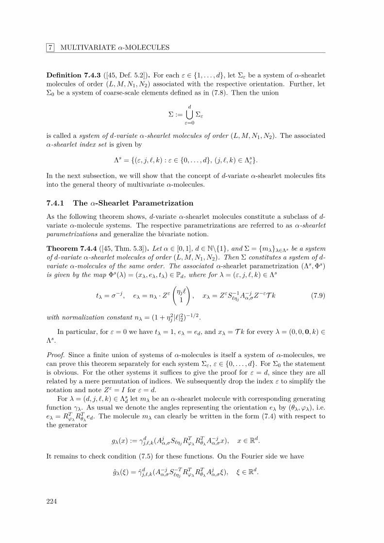
7 MULTIVARIATE α-MOLECULES
Definition 7.4.3 ([45, Def. 5.2]). For each ε ∈ 1, . . . , d, let Σε be a system of α-shearletmolecules of order (L,M,N1, N2) associated with the respective orientation. Further, letΣ0 be a system of coarse-scale elements defined as in (7.8). Then the union
Σ :=d
ε=0Σε
is called a system of d-variate α-shearlet molecules of order (L,M,N1, N2). The associatedα-shearlet index set is given by
Λs = (ε, j, ℓ, k) : ε ∈ 0, . . . , d, (j, ℓ, k) ∈ Λsε.
In the next subsection, we will show that the concept of d-variate α-shearlet molecules fitsinto the general theory of multivariate α-molecules.
7.4.1 The α-Shearlet Parametrization
As the following theorem shows, d-variate α-shearlet molecules constitute a subclass of d-variate α-molecule systems. The respective parametrizations are referred to as α-shearletparametrizations and generalize the bivariate notion.
Theorem 7.4.4 ([45, Thm. 5.3]). Let α ∈ [0, 1], d ∈ N\1, and Σ = mλλ∈Λs be a systemof d-variate α-shearlet molecules of order (L,M,N1, N2). Then Σ constitutes a system of d-variate α-molecules of the same order. The associated α-shearlet parametrization (Λs,Φs)is given by the map Φs(λ) = (xλ, eλ, tλ) ∈ Pd, where for λ = (ε, j, ℓ, k) ∈ Λs
tλ = σ−j , eλ = nλ · Zε
ηjℓ1
, xλ = ZεS−1
ℓηjA−j
α,σZ−εT k (7.9)
with normalization constant nλ = (1 + η2j |ℓ|22)−1/2.
In particular, for ε = 0 we have tλ = 1, eλ = ed, and xλ = T k for every λ = (0, 0,0, k) ∈Λs.
Proof. Since a finite union of systems of α-molecules is itself a system of α-molecules, wecan prove this theorem separately for each system Σε, ε ∈ 0, . . . , d. For Σ0 the statementis obvious. For the other systems it suffices to give the proof for ε = d, since they are allrelated by a mere permutation of indices. We subsequently drop the index ε to simplify thenotation and note Zε = I for ε = d.
For λ = (d, j, ℓ, k) ∈ Λsd let mλ be an α-shearlet molecule with corresponding generating
function γλ. As usual we denote the angles representing the orientation eλ by (θλ, ϕλ), i.e.eλ = RT
ϕλRT
θλed. The molecule mλ can clearly be written in the form (7.4) with respect to
the generator
gλ(x) := γdj,ℓ,k(Aj
α,σSℓηjRT
ϕλRT
θλA−j
α,σx), x ∈ Rd.
It remains to check condition (7.5) for these functions. On the Fourier side we have
gλ(ξ) = γdj,ℓ,k(A−j
α,σS−TℓηjRT
ϕλRT
θλAj
α,σξ), ξ ∈ Rd.
224
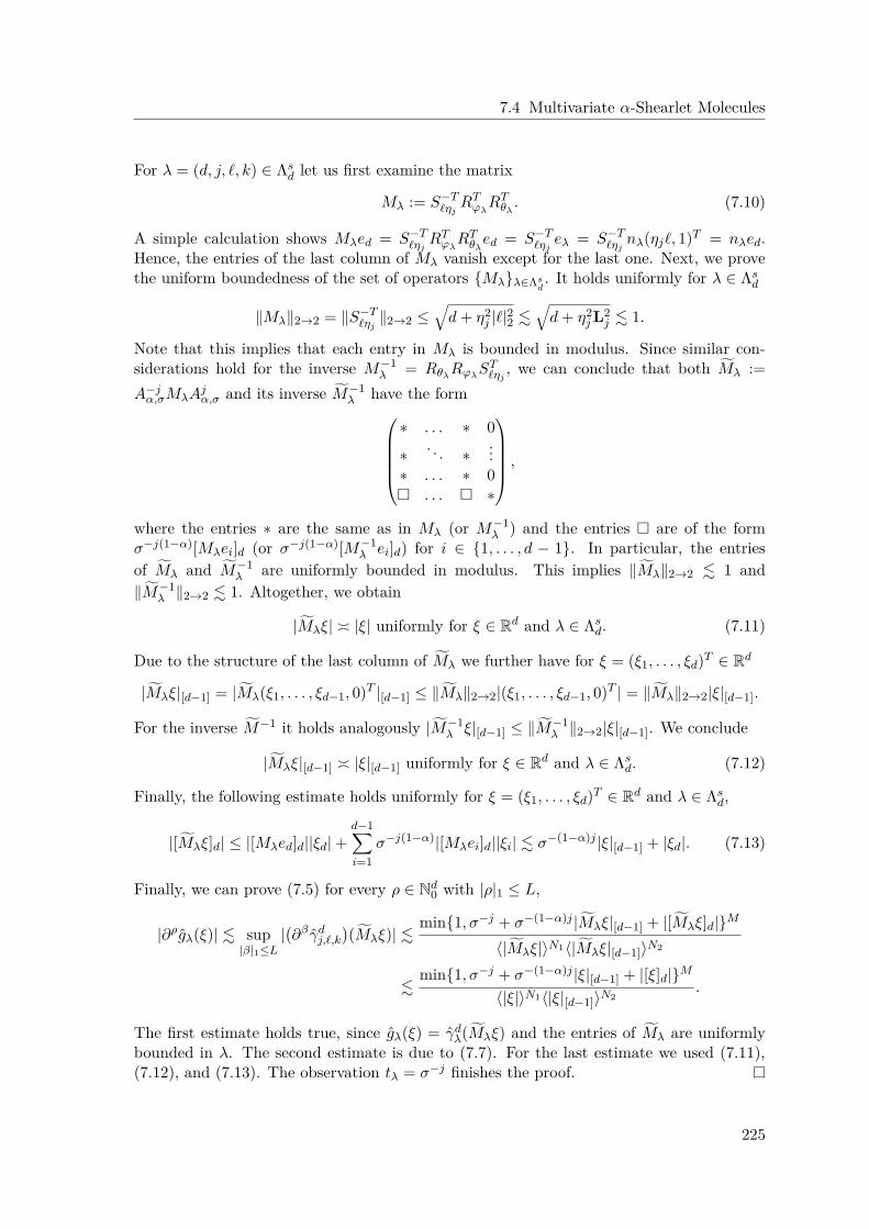
7.4 Multivariate α-Shearlet Molecules
For λ = (d, j, ℓ, k) ∈ Λsd let us first examine the matrix
Mλ := S−TℓηjRT
ϕλRT
θλ. (7.10)
A simple calculation shows Mλed = S−TℓηjRT
ϕλRT
θλed = S−T
ℓηjeλ = S−T
ℓηjnλ(ηjℓ, 1)T = nλed.
Hence, the entries of the last column of Mλ vanish except for the last one. Next, we provethe uniform boundedness of the set of operators Mλλ∈Λs
d. It holds uniformly for λ ∈ Λs
d
∥Mλ∥2→2 = ∥S−Tℓηj
∥2→2 ≤d+ η2
j |ℓ|22 .d+ η2
j L2j . 1.
Note that this implies that each entry in Mλ is bounded in modulus. Since similar con-siderations hold for the inverse M−1
λ = RθλRϕλ
STℓηj, we can conclude that both Mλ :=
A−jα,σMλA
jα,σ and its inverse M−1
λ have the form∗ . . . ∗ 0
∗ . . . ∗...
∗ . . . ∗ 0 . . . ∗
,where the entries ∗ are the same as in Mλ (or M−1
λ ) and the entries are of the formσ−j(1−α)[Mλei]d (or σ−j(1−α)[M−1
λ ei]d) for i ∈ 1, . . . , d − 1. In particular, the entriesof Mλ and M−1
λ are uniformly bounded in modulus. This implies ∥Mλ∥2→2 . 1 and∥M−1
λ ∥2→2 . 1. Altogether, we obtain
|Mλξ| ≍ |ξ| uniformly for ξ ∈ Rd and λ ∈ Λsd. (7.11)
Due to the structure of the last column of Mλ we further have for ξ = (ξ1, . . . , ξd)T ∈ Rd
|Mλξ|[d−1] = |Mλ(ξ1, . . . , ξd−1, 0)T |[d−1] ≤ ∥Mλ∥2→2|(ξ1, . . . , ξd−1, 0)T | = ∥Mλ∥2→2|ξ|[d−1].
For the inverse M−1 it holds analogously |M−1λ ξ|[d−1] ≤ ∥M−1
λ ∥2→2|ξ|[d−1]. We conclude
|Mλξ|[d−1] ≍ |ξ|[d−1] uniformly for ξ ∈ Rd and λ ∈ Λsd. (7.12)
Finally, the following estimate holds uniformly for ξ = (ξ1, . . . , ξd)T ∈ Rd and λ ∈ Λsd,
|[Mλξ]d| ≤ |[Mλed]d||ξd| +d−1i=1
σ−j(1−α)|[Mλei]d||ξi| . σ−(1−α)j |ξ|[d−1] + |ξd|. (7.13)
Finally, we can prove (7.5) for every ρ ∈ Nd0 with |ρ|1 ≤ L,
|∂ρgλ(ξ)| . sup|β|1≤L
|∂β γd
j,ℓ,k
(Mλξ)| .
min1, σ−j + σ−(1−α)j |Mλξ|[d−1] + |[Mλξ]d|M
⟨|Mλξ|⟩N1⟨|Mλξ|[d−1]⟩N2
.min1, σ−j + σ−(1−α)j |ξ|[d−1] + |[ξ]d|M
⟨|ξ|⟩N1⟨|ξ|[d−1]⟩N2.
The first estimate holds true, since gλ(ξ) = γdλ(Mλξ) and the entries of Mλ are uniformly
bounded in λ. The second estimate is due to (7.7). For the last estimate we used (7.11),(7.12), and (7.13). The observation tλ = σ−j finishes the proof.
225
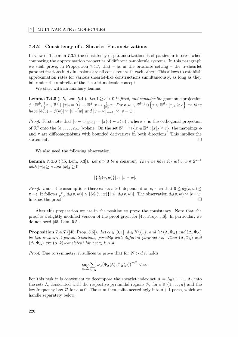
7 MULTIVARIATE α-MOLECULES
7.4.2 Consistency of α-Shearlet Parametrizations
In view of Theorem 7.3.2 the consistency of parametrizations is of particular interest whencomparing the approximation properties of different α-molecule systems. In this paragraphwe shall prove, in Proposition 7.4.7, that – as in the bivariate setting – the α-shearletparametrizations in d dimensions are all consistent with each other. This allows to establishapproximation rates for various shearlet-like constructions simultaneously, as long as theyfall under the umbrella of the shearlet-molecule concept.
We start with an auxiliary lemma.
Lemma 7.4.5 ([45, Lem. 5.4]). Let 1 ≥ c > 0 be fixed, and consider the gnomonic projectionφ : Rd\
x ∈ Rd | [x]d = 0
→ Rd, x →→ 1
[x]dx. For v, w ∈ Sd−1 ∩x ∈ Rd : [x]d ≥ c
we then
have |φ(v) − φ(w)| ≍ |v − w| and |v − w|[d−1] ≍ |v − w|.
Proof. First note that |v − w|[d−1] = |π(v) − π(w)|, where π is the orthogonal projectionof Rd onto the (e1, . . . , ed−1)-plane. On the set Sd−1 ∩
x ∈ Rd : [x]d ≥ c
, the mappings φ
and π are diffeomorphisms with bounded derivatives in both directions. This implies thestatement.
We also need the following observation.
Lemma 7.4.6 ([45, Lem. 6.3]). Let c > 0 be a constant. Then we have for all v, w ∈ Sd−1
with [v]d ≥ c and [w]d ≥ 0
|dS(v, w)| ≍ |v − w|.
Proof. Under the assumptions there exists ε > 0 dependent on c, such that 0 ≤ dS(v, w) ≤π−ε. It follows ε
π−ε |dS(v, w)| ≤ |dS(v, w)| ≤ |dS(v, w)|. The observation dS(v, w) ≍ |v−w|finishes the proof.
After this preparation we are in the position to prove the consistency. Note that theproof is a slightly modified version of the proof given for [45, Prop. 5.6]. In particular, wedo not need [45, Lem. 5.5].
Proposition 7.4.7 ([45, Prop. 5.6]). Let α ∈ [0, 1], d ∈ N\1, and let (Λ,ΦΛ) and (∆,Φ∆)be two α-shearlet parametrizations, possibly with different parameters. Then (Λ,ΦΛ) and(∆,Φ∆) are (α, k)-consistent for every k > d.
Proof. Due to symmetry, it suffices to prove that for N > d it holds
supµ∈∆
λ∈Λ
ωαΦΛ(λ),Φ∆(µ)
−N< ∞.
For this task it is convenient to decompose the shearlet index set Λ = Λ0 ∪ · · · ∪ Λd intothe sets Λε associated with the respective pyramidal regions Pε for ε ∈ 1, . . . , d and thelow-frequency box R for ε = 0. The sum then splits accordingly into d+ 1 parts, which wehandle separately below.
226
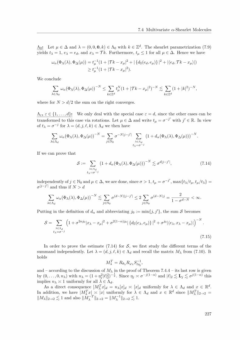
7.4 Multivariate α-Shearlet Molecules
Λ0: Let µ ∈ ∆ and λ = (0, 0,0, k) ∈ Λ0 with k ∈ Zd. The shearlet parametrization (7.9)yields tλ = 1, eλ = ed, and xλ = T k. Furthermore, tµ ≤ 1 for all µ ∈ ∆. Hence we have
ωαΦΛ(λ),Φ∆(µ)
= t−1
µ (1 + |T k − xµ|2 + | dS(ed, eµ) |2 + |⟨ed, T k − xµ⟩|)≥ t−1
µ (1 + |T k − xµ|2).
We concludeλ∈Λ0
ωαΦΛ(λ),Φ∆(µ)
−N ≤
k∈Zd
tNµ (1 + |T k − xµ|2)−N .
k∈Zd
(1 + |k|2)−N ,
where for N > d/2 the sum on the right converges.
Λε, ε ∈ 1, . . . , d: We only deal with the special case ε = d, since the other cases can betransformed to this case via rotations. Let µ ∈ ∆ and write tµ = σ−j′ with j′ ∈ R. In viewof tλ = σ−j for λ = (d, j, ℓ, k) ∈ Λd we then have
λ∈Λd
ωαΦΛ(λ),Φ∆(µ)
−N =
j∈N0
σ−N |j−j′| λ∈Λd
tλ=σ−j
1 + dα
ΦΛ(λ),Φ∆(µ)
−N.
If we can prove that
S :=
λ∈Λdtλ=σ−j
1 + dα
ΦΛ(λ),Φ∆(µ)
−N. σd|j−j′|, (7.14)
independently of j ∈ N0 and µ ∈ ∆, we are done, since σ > 1, tµ = σ−j′ , maxtλ/tµ, tµ/tλ =σ|j−j′| and thus if N > d
λ∈Λd
ωαΦΛ(λ),Φ∆(µ)
−N.
j∈N0
σ(d−N)|j−j′| ≤ 2
j∈N0
σ(d−N)j = 21 − σd−N
< ∞.
Putting in the definition of dα and abbreviating j0 := minj, j′, the sum S becomes
S =
λ∈Λdtλ=σ−j
1 + σ2αj0 |xλ − xµ|2 + σ2(1−α)j0 | dS(eλ, eµ) |2 + σj0 |⟨eλ, xλ − xµ⟩|
−N.
(7.15)
In order to prove the estimate (7.14) for S, we first study the different terms of thesummand independently. Let λ = (d, j, ℓ, k) ∈ Λd and recall the matrix Mλ from (7.10). Itholds
MTλ = Rθλ
RϕλS−1
ℓηj,
and – according to the discussion of Mλ in the proof of Theorem 7.4.4 – its last row is givenby (0, . . . , 0, nλ) with nλ = (1 + η2
j |ℓ|22)− 12 . Since ηj ≍ σ−j(1−α) and |ℓ|2 . Lj . σj(1−α) this
implies nλ ≍ 1 uniformly for all λ ∈ Λd.As a direct consequence [MT
λ x]d = nλ[x]d ≍ [x]d uniformly for λ ∈ Λd and x ∈ Rd.In addition, we have |MT
λ x| ≍ |x| uniformly for λ ∈ Λd and x ∈ Rd since ∥MTλ ∥2→2 =
∥Mλ∥2→2 . 1 and also ∥M−Tλ ∥2→2 = ∥M−1
λ ∥2→2 . 1.
227
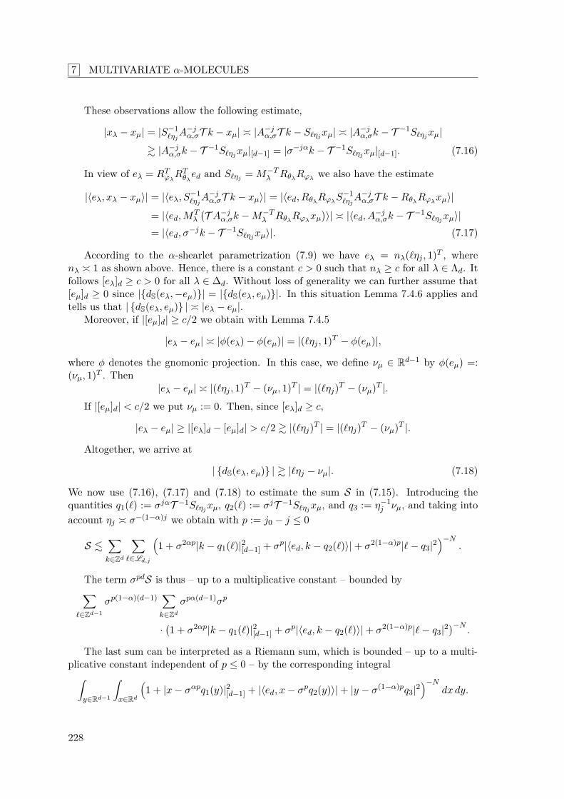
7 MULTIVARIATE α-MOLECULES
These observations allow the following estimate,
|xλ − xµ| = |S−1ℓηjA−j
α,σT k − xµ| ≍ |A−jα,σT k − Sℓηj
xµ| ≍ |A−jα,σk − T −1Sℓηj
xµ|
& |A−jα,σk − T −1Sℓηj
xµ|[d−1] = |σ−jαk − T −1Sℓηjxµ|[d−1]. (7.16)
In view of eλ = RTϕλRT
θλed and Sℓηj
= M−Tλ Rθλ
Rϕλwe also have the estimate
|⟨eλ, xλ − xµ⟩| = |⟨eλ, S−1ℓηjA−j
α,σT k − xµ⟩| = |⟨ed, RθλRϕλ
S−1ℓηjA−j
α,σT k −RθλRϕλ
xµ⟩|
= |⟨ed,MTλ
T A−j
α,σk −M−Tλ Rθλ
Rϕλxµ⟩| ≍ |⟨ed, A
−jα,σk − T −1Sℓηj
xµ⟩|= |⟨ed, σ
−jk − T −1Sℓηjxµ⟩|. (7.17)
According to the α-shearlet parametrization (7.9) we have eλ = nλ(ℓηj , 1)T , wherenλ ≍ 1 as shown above. Hence, there is a constant c > 0 such that nλ ≥ c for all λ ∈ Λd. Itfollows [eλ]d ≥ c > 0 for all λ ∈ ∆d. Without loss of generality we can further assume that[eµ]d ≥ 0 since |dS(eλ,−eµ)| = |dS(eλ, eµ)|. In this situation Lemma 7.4.6 applies andtells us that | dS(eλ, eµ) | ≍ |eλ − eµ|.
Moreover, if |[eµ]d| ≥ c/2 we obtain with Lemma 7.4.5
|eλ − eµ| ≍ |φ(eλ) − φ(eµ)| = |(ℓηj , 1)T − φ(eµ)|,
where φ denotes the gnomonic projection. In this case, we define νµ ∈ Rd−1 by φ(eµ) =:(νµ, 1)T . Then
|eλ − eµ| ≍ |(ℓηj , 1)T − (νµ, 1)T | = |(ℓηj)T − (νµ)T |.
If |[eµ]d| < c/2 we put νµ := 0. Then, since [eλ]d ≥ c,
|eλ − eµ| ≥ |[eλ]d − [eµ]d| > c/2 & |(ℓηj)T | = |(ℓηj)T − (νµ)T |.
Altogether, we arrive at
| dS(eλ, eµ) | & |ℓηj − νµ|. (7.18)
We now use (7.16), (7.17) and (7.18) to estimate the sum S in (7.15). Introducing thequantities q1(ℓ) := σjαT −1Sℓηj
xµ, q2(ℓ) := σjT −1Sℓηjxµ, and q3 := η−1
j νµ, and taking intoaccount ηj ≍ σ−(1−α)j we obtain with p := j0 − j ≤ 0
S .
k∈Zd
ℓ∈Ld,j
1 + σ2αp|k − q1(ℓ)|2[d−1] + σp|⟨ed, k − q2(ℓ)⟩| + σ2(1−α)p|ℓ− q3|2
−N.
The term σpdS is thus – up to a multiplicative constant – bounded byℓ∈Zd−1
σp(1−α)(d−1) k∈Zd
σpα(d−1)σp
·1 + σ2αp|k − q1(ℓ)|2[d−1] + σp|⟨ed, k − q2(ℓ)⟩| + σ2(1−α)p|ℓ− q3|2
−N.
The last sum can be interpreted as a Riemann sum, which is bounded – up to a multi-plicative constant independent of p ≤ 0 – by the corresponding integral
y∈Rd−1
x∈Rd
1 + |x− σαpq1(y)|2[d−1] + |⟨ed, x− σpq2(y)⟩| + |y − σ(1−α)pq3|2
−Ndx dy.
228
7.5 Application: Sparse Approximation of Video Data
All in all we end up with
S . σd(j−j0)
y∈Rd−1
x∈Rd
1 + |x|2[d−1] + |⟨ed, x⟩| + |y|2
−Ndx dy.
To see that the integral converges for N > d, we carry out the integration over xd, whichyields up to a fixed constant
y∈Rd−1
x∈Rd−1
(1 + |x|2[d−1] + |y|2)−(N−1) dx dy =
z∈R2(d−1)(1 + |z|2)−(N−1).
The integral on the right converges precisely for N > d. This observation concludes theproof.
7.5 Application: Sparse Approximation of Video Data
In this section, we will demonstrate with a specific example how the machinery of d-variateα-molecules can be applied in practice. In our exemplary application, we are interested inthe sparse approximation of video signals modelled by the class of cartoon-like functionsE2([0, 1]3, ν) introduced below.
Following the general methodology of the transfer principle, we just need to find asuitable anchor system for which a sparse approximation result with respect to E2([0, 1]3, ν)is known. Utilizing Theorem 7.3.2, the framework can then transfer the approximation ratefrom this anchor system to other systems. In this way, we will identify a large class ofrepresentation systems providing almost optimal sparse approximation for E2([0, 1]3, ν).
7.5.1 Cartoon-like Functions in 3D
A suitable model for video data is provided by a 3-dimensional version of the original classof cartoon-like functions introduced by Donoho in [38], namely the following model definedin [83].
Definition 7.5.1 ([38],[83, Def 2.1]). For fixed ν > 0, the class E2([0, 1]3, ν) of cartoon-likefunctions consists of functions f : R3 → C of the form
f = f0 + f1XB,
where B ⊂ [0, 1]3 and fi ∈ C2(R3) with supp fi ⊂ [0, 1]3 and ∥fi∥C2 ≤ ν for each i = 0, 1.Further, the discontinuity ∂B shall be a closed C2-surface with principal curvatures boundedby ν.
This model is justified by the observation that real-life video data, just like real-life imagedata, typically consists of smooth regions, separated by piecewise smooth boundaries. Notehowever that for simplicity we restrict to cartoon-like functions with smooth boundaries inDefinition 7.5.1.
229
7 MULTIVARIATE α-MOLECULES
7.5.2 Pyramid-adapted Shearlet Systems in 3D
In the sequel, we will present some concrete shearlet systems in 3 dimensions which arealready on the market. Thereby we restrict our attention to parabolically scaled systems.
In the classic sense [79], a shearlet system in L2(R3) refers to a collection of functionsof the form
ψj,ℓ,k = 2jψ(SℓAj12 ,2 · −k) : j ∈ Z, ℓ ∈ Z2, k ∈ Z3
, (7.19)
where ψ ∈ L2(R3) is some suitable generator. The classic choice for ψ is furthermore afunction defined on the frequency domain by
ψ(ξ) = w(ξ3)v( ξ1ξ3
)v( ξ2ξ3
), ξ = (ξ1, ξ2, ξ3)T ∈ R3,
where v ∈ C∞c (R) is a bump function and w ∈ C∞
c (R) is the Fourier transform of a suitableunivariate discrete wavelet. It was shown in [79] that it is possible to choose v and w sothat (7.19) becomes a Parseval frame for L2(R3).
Unfortunately, the shearlet system (7.19) is directionally biased due to the fact that forlarge shearings the frequency support of the shearlets becomes more and more elongatedalong the (e1, e2)-plane. This bias has a negative effect on the approximation propertiesand makes the system (7.19) impractical for most applications.
To avoid this problem, the Fourier domain is partitioned into three pyramidal regionssimilar to the two cones in 2 dimensions,
P1 =
(ξ1, ξ2, ξ3) ∈ R3 : | ξ2ξ1
| ≤ 1, | ξ3ξ1
| ≤ 1,
P2 =
(ξ1, ξ2, ξ3) ∈ R3 : | ξ1ξ2
| ≤ 1, | ξ3ξ2
| ≤ 1,
P3 =
(ξ1, ξ2, ξ3) ∈ R3 : | ξ1ξ3
| ≤ 1, | ξ2ξ3
| ≤ 1.
Then, for each pyramid a separate shearlet system can be used and, since each system nowonly has to cover one pyramid, large shears are avoided. To take care of low frequencies,as in the 2-dimensional case, it is common to use distinguished coarse-scale elements withfrequencies in a centered box around the origin. Subsequently, it will be the cube
R =ξ ∈ R3 : |ξ|∞ ≤ 1
8
.
Note that this cube together with the truncated pyramids P1 := P1\R, P2 := P2\R, andP3 := P3\R partitions the Fourier domain into 4 distinct regions.
With each of these regions, different operators are associated. The coarse-scale functionsare only translated, in the other regions we also scale and shear. The scaling and shearingoperators associated with the respective regions ε ∈ 1, 2, 3 are given by A(ε)
12 ,t
= ZεA 12 ,tZ
−ε
and S(ε)h = ZεShZ
−ε, and take the concrete form
A(1)12 ,t
=
t 0 00 t
12 0
0 0 t12
, A(2)12 ,t
=
t12 0 00 t 00 0 t
12
, A(3)12 ,t
= Aα,s =
t12 0 00 t
12 0
0 0 t
,
230
7.5 Application: Sparse Approximation of Video Data
for t > 0, and for h ∈ R2
S(1)h =
1 h1 h20 1 00 0 1
, S(2)h =
1 0 0h2 1 h10 0 1
, S(3)h = Sh =
1 0 00 1 0h1 h2 1
.Now we are ready to define a modified shearlet system, which is adapted to our partition
of the Fourier domain and therefore called pyramid-adapted. This system does not exhibitthe directional bias as (7.19) and can be considered as a 3D-version of the cone-adaptedshearlet system from Definition 3.3.8.
Definition 7.5.2 ([83, 82]). For fixed τ1, τ2 > 0 let T = diag(τ1, τ2, τ2) ∈ R3×3. The(affine) pyramid-adapted 3D shearlet system generated by the functions φ ∈ L2(R3) andψε ∈ L2(R3), ε ∈ 1, 2, 3, is defined as the union
SH(φ, ψ1, ψ2, ψ3; τ1, τ2) := Φ(φ; τ1) ∪ Ψ1(ψ1; τ1, τ2) ∪ Ψ2(ψ2; τ1, τ2) ∪ Ψ3(ψ3; τ1, τ2) (7.20)
of the coarse-scale functions Φ(φ; τ1) := φk = φ(· − τ1k) : k ∈ Z3 and the functions
Ψε(ψε; τ1, τ2) :=ψε
j,ℓ,k : j ∈ N0, ℓ ∈ Z2, |ℓ|∞ ≤ ⌈2j/2⌉, k ∈ Z3,
associated with the pyramids Pε for ε ∈ 1, 2, 3, which are given by
ψεj,ℓ,k := 2jψε(ZεSℓA
j12 ,2Z
−ε · −ZεT Z−εk).
These pyramid-adapted affine systems are the prime examples of 12 -shearlet-molecules.
In practice, one usually wants them to be frames, or even Parseval or tight frames. However,ensuring the frame property of pyramid-adapted shearlets is not trivial.
Frames of Pyramid-adapted Shearlets
The simplest way to obtain a Parseval frame of pyramid-adapted shearlets builds upon aParseval shearlet frame of the type (7.19), which is easier to construct. A shearlet systemassociated with the pyramid P3 is then obtained by removing all elements, whose frequencysupport does not intersect P3. Truncating the remaining functions in the frequency domainoutside of P3, one obtains a Parseval frame for the space
L2(P3)∨ := f ∈ L2(R3) : supp f ⊂ P3.
A similar procedure yields Parseval frames associated with the the other parts of the Fourierdomain, namely for L2(Pε)∨, ε ∈ 1, 2, and L2(R)∨. The union of these frames then is aParseval frame for the whole space L2(R3).
This approach has the drawback that it leads to bad spatial localization of the shearletsdue to their lack of smoothness in the frequency domain, which is a consequence of thetruncation. A different approach was taken by Candès, Demanet, and Ying in [115]. Theygave up on the affine structure of the system and could then find a shearlet-type constructionwith the Parseval property. Guo and Labate later modified this approach [69, 70] and foundanother shearlet-type construction, which is even close to affine.
We will subsequently denote this system by SH. It is a Parseval frame of band-limitedshearlets for L2(R3). Moreover, it is a system of 1
2 -molecules.
231
7 MULTIVARIATE α-MOLECULES
Proposition 7.5.3 ([45, Prop. 5.9]). Appropriately re-indexed, the smooth Parseval frameof band-limited 3D-shearlets SH constructed in [69] constitutes a system of 3-dimensional12 -shearlet molecules of order (∞,∞,∞,∞).
In particular, SH is a system of 3-dimensional 12 -molecules of order (∞,∞,∞,∞). The
associated parametrization (ΛSH ,ΦSH) is given explicitly in [45, Cor. 5.10]. It is related toa 1
2 -shearlet parametrization by a mere relabelling of the shearlets.
Remark 7.5.4 ([45, Rem. 5.11]). Although (ΛSH ,ΦSH) is not a shearlet parametriza-tion, it is (1
2 , k)-consistent with every 12 -shearlet parametrization for k > 3. This follows
from Proposition 7.4.7 and the observation that relabelling of elements does not make anydifference.
There also exist shearlet frames for L2(R3) consisting of compactly supported functions.Such frames have been constructed for example in [83]. As the following proposition shows,they are also instances of 1
2 -shearlet molecules and their order can be controlled by theregularity of the generators.
Proposition 7.5.5 ([45, Prop. 5.12]). Let φ, ψ1, ψ2, ψ3 ∈ L2(R3) be compactly supportedand L,M,N1, N2 ∈ N0 ∪ ∞. If φ ∈ CN1+N2(R3) and if, for every ε ∈ 1, 2, 3,
(i) the derivatives ∂γψε exist and are continuous for every γ ∈ N30 with [Zεγ]1, [Zεγ]2 ≤
N1 +N2 and [Zεγ]3 ≤ N1, where Z is the cyclic permutation matrix (7.6),
(ii) the generator ψε has M + L directional vanishing moments in eε-direction, i.e.
∀(x1, x2) ∈ R2 :Rψε(Zεx)xN
3 dx3 = 0 for every N ∈ 0, . . . ,M + L− 1,
then the system (7.20) obtained from these generators is a system of 12 -shearlet molecules
of order (L,M,N1, N2).
Proof. Due to the assumptions, the generators are functions in Cc(R3) and hence in par-ticular contained in L1(R3). As a consequence, their Fourier transforms φ, ψ1, ψ2, ψ3 arebounded. Hence, rightly indexed, the induced system of the form (7.20) constitutes a sys-tem of 1
2 -shearlet molecules. It remains to verify the order of the system. For this, littlemore is needed than utilizing the facts that spatial decay implies smoothness in Fourierdomain (and vice versa), and that vanishing moments in spatial domain implies estimatesof the form |g(ξ)| . min(1, |ξ|)M in Fourier domain. We refer to [62, Prop. 3.11] for details,where a similar two-dimensional version of the theorem is proven.
7.5.3 Quasi-Optimal Approximation with 3D Parabolic Molecules
In [83] the optimal approximation rate under a polynomial depth search constraint forE2([0, 1]3, ν) was derived. Recall that a dictionary-based algorithm for sparse approxima-tion is said to satisfy a polynomial depth search constraint if there exists a polynomial πsuch that the algorithm only chooses from the first π(N) dictionary elements when formingthe N :th sparse approximation [38]. If such a constraint is not assumed, one could forinstance use the whole of E2([0, 1]3, ν) as a dictionary yielding 1-sparse representations for
232
7.5 Application: Sparse Approximation of Video Data
any element of E2([0, 1]3, ν). But clearly, those have no practical relevance for real-worldapproximation schemes.
The following benchmark for E2([0, 1]3, ν) was proved in [83] with the same techniquesused in Section 5.3.
Theorem 7.5.6 ([38, Thm 7.2],[83, Thm 3.2]). The best N -term approximation rate forE2([0, 1]3, ν), achieved by an arbitrary dictionary under the restriction of polynomial depthsearch, cannot exceed
∥f − fN ∥22 . N−1,
where fN is the best N -term approximation of f ∈ E2([0, 1]3, ν).
There are several examples of frames which almost provide these optimal rates [69, 83],typically up to log-terms. In particular, it was proven by Guo and Labate [69] that thesmooth Parseval frame of 3D-shearlets SH sparsely approximates this class. The obtainedapproximation result is stated below in (7.21). It is based on the following estimate for thesize of the shearlet coefficients.
Theorem 7.5.7 ([69, Thm 3.1]). Let SH = ψλλ∈Λs be the smooth Parseval frame of3D-shearlets defined in [70]. Then the sequence of shearlet coefficients θλ(f) := ⟨f, ψλ⟩,λ ∈ Λs, associated with f ∈ E2([0, 1]3, ν) satisfies
supf∈E2([0,1]3,ν)
|θλ(f)|N . N−1 · log(N),
where |θλ(f)|N denotes the N :th largest shearlet coefficient.
Theorem 7.5.7 shows that the shearlet coefficients belong to ωℓp(Λs) for every p > 1. Inview of Lemma 2.3.1, for every f ∈ E2([0, 1]3, ν), the frame SH therefore provides at leastthe approximation rate
∥f − fN ∥22 . N−1+ε , ε > 0 arbitrary, (7.21)
where fN denotes the N -term approximation obtained from the N largest coefficients. Ac-cording to Theorem 7.5.6, this is almost the optimal approximation rate achievable forcartoon-like functions E2([0, 1]3, ν). For small ε > 0, we get arbitrarily close to the optimalrate.
Transfer of the Approximation Rate
We now come to our final goal of identifying a large class of representation systems whichachieve the almost optimal rate (7.21) for the class E2([0, 1]3, ν). For this, we put themachinery of α-molecules to work. Concretely, we use Theorem 7.3.2 to transfer the ap-proximation rate (7.21) of the smooth Parseval frame of 3D-shearlets SH to other systemsof 3-dimensional 1
2 -molecules. This leads to the following result, whereby (ΛSH ,ΦSH) shalldenote the parametrization of SH.
Theorem 7.5.8 ([45, Thm. 4.4]). Assume that a frame mλλ∈Λ of 3-dimensional parabolicmolecules satisfies, for some k > 0, the following two conditions:
(i) its parametrization (Λ,ΦΛ) is (12 , k)-consistent with (ΛSH ,ΦSH),
233
7 MULTIVARIATE α-MOLECULES
(ii) its order (L,M,N1, N2) satisfies
L ≥ 2k, M ≥ 3k − 2, N1 ≥ k + 1, N1 > 3/2, N2 ≥ 2k + 1.
Then each dual frame mλλ∈Λ possesses an almost optimal N -term approximation rate forthe class of cartoon-like functions E2([0, 1]3, ν), i.e., for all f ∈ E2([0, 1]3, ν)
∥f − fN ∥22 . N−1+ε, ε > 0 arbitrary,
where fN denotes the N -term approximation obtained from the N largest frame coefficients.
Proof. The proof is analogous to the proof of Theorem 6.0.2. Due to Proposition 7.5.3, theframe SH is a system of 3-dimensional 1
2 -molecules of order (∞,∞,∞,∞). It is thus asuitable reference system for the application of the transfer principle, Theorem 7.3.2. Theassertion then follows from Theorem 7.5.7.
Theorem 7.5.8 specifies a large class of multiscale systems with almost optimal approx-imation performance for video data in the class E2([0, 1]3, ν). According to Remark 7.5.4,condition (i) is in particular fulfilled by every 1
2 -shearlet parametrization (see Section 7.4)for k > 3. Hence, due to condition (ii), all systems of 3-dimensional 1
2 -shearlet molecules oforder
L ≥ 7, M ≥ 8, N1 ≥ 5, N2 ≥ 8,
provide almost optimal approximation for E2([0, 1]3, ν).Taking into account Proposition 7.5.5, the statement of Theorem 7.5.8 in particular
includes the following result for compactly supported shearlet frames.
Corollary 7.5.9 ([45, Cor. 4.5]). Any dual frame of a shearlet frame of the form (7.20)generated by compactly supported functions φ, ψ1, ψ2, ψ3 ∈ L2(R3), so that φ ∈ C13(R3) andfor each permutation (i, j, k) of (1, 2, 3), we have
(i) ∂γψi exists and is continuous for every γ ∈ N30 with γi ≤ 5 and γj , γk ≤ 13,
(ii) ψi has at least 15 vanishing directional moments in direction ei,
provides the almost optimal approximation rate (7.21) for the cartoon class E2([0, 1]3, ν).
A result similar to this corollary was proved in [83]. In comparison, the most intriguingfact about this corollary is the simplicity of its deduction. The framework of α-moleculesenables a simple transfer of the decay rates.
7.6 Appendix: Proof of Theorem 7.2.2
This section is devoted to the proof of Theorem 7.2.2. The exposition is essentially thesame as in [45, Sec. 6]. It is split into several parts and has the same general structure asthe proof of Theorem 2.2.2 in Section 2.5. Let us first collect some simple elementary facts,which turn out to be useful.
234
7.6 Appendix: Proof of Theorem 7.2.2
7.6.1 Auxiliary Lemmas
Subsequently O(d,R) shall denote the orthogonal group of Rd. Further, recall the ‘projec-tion’ θ of θ ∈ R onto the interval T := [−π
2 ,π2 ) defined in (2.9). Recall also the notation
dS(v, w) for the angle arccos(⟨v, w⟩) ∈ [0, π] between two vectors v, w ∈ Sd−1.An immediate corollary of Lemma 2.5.1 is the following result.
Lemma 7.6.1 ([45, Lem. 6.2]). Let ed ∈ Rd be the d:th unit vector. For η ∈ Sd−1 we have| dS(η, ed) | ≍ |η|[d−1].
Proof. Using a suitable rotation R ∈ O(d,R) of the form
R =Rd−1 0
0 1
,
where Rd−1 ∈ O(d−1,R), we can achieve Rη = (sin(θ), 0, . . . , 0, cos(θ))T with θ = dS(η, ed).Since |η|[d−1] = |η− ed|[d−1] = |R(η− ed)|[d−1] = |Rη− ed|[d−1] = | sin(θ)|, it just remains toprove | sin(θ)| ≍ | θ |, which is true by Lemma 2.5.1.
We will further need the lemma below.
Lemma 7.6.2 ([45, Lem. 6.4]). Let R ∈ O(d,R) be a rotation and θ0 = dS(ed, Red) ∈ [0, π]the angle between the d:th unit vector ed ∈ Rd and its image Red under R. Then it holdsfor all η ∈ Sd−1
|Rη|[d−1] = sin(dS(Rη, ed)) ≥ min| sin(dS(η, ed) + θ0)|, | sin(dS(η, ed) − θ0)|.
Note dS(η, ed) = dS(Rη,Red).
Proof. Let η = (η1, . . . , ηd)T ∈ Sd−1 and put θ1 := dS(η, ed) = arccos(⟨η, ed⟩) ∈ [0, π]. Therotation R ∈ O(d,R) can be decomposed in the form R = RRθ0 with R, Rθ0 ∈ O(d,R) suchthat
R =Rd−1
1
and Rθ0 =
cos(θ0) − sin(θ0)Id−2
sin(θ0) cos(θ0)
,where Rd−1 ∈ O(d − 1,R) is some (d − 1)-dimensional rotation matrix and Id−2 is the(d− 2)-dimensional identity matrix. The rotation R leaves | · |[d−1] invariant, whence
|Rη|[d−1] = |RRθ0η|[d−1] = |Rθ0η|[d−1].
Using ηd = cos(θ1) and |η|2[d−1] = η21 + η2
2 + . . .+ η2d−1 = 1 − η2
d, it further follows
|Rθ0η|2[d−1] = (cos(θ0)η1 − sin(θ0)ηd)2 + η22 + · · · + η2
d−1
= cos2(θ0)η21 + sin2(θ0) cos2(θ1) − 2 cos(θ0) sin(θ0)η1 cos(θ1) + (1 − η2
1 − cos2(θ1))= 1 − (η1 sin(θ0) + cos(θ1) cos(θ0))2.
The last expression is a second-degree polynomial in the variable η1 with a negative leadingcoefficient. Since η2
1 ≤ 1 − η2d = 1 − cos2(θ1) = sin2(θ1), the variable η1 can take values only
235
7 MULTIVARIATE α-MOLECULES
in [− sin(θ1), sin(θ1)]. The polynomial attains its minimum on this interval at the endpoints.Hence, we can conclude
|Rθ0η|2[d−1] ≥ minϵ∈−1,1
1 − (ϵ sin(θ1) sin(θ0) + cos(θ1) cos(θ0))2
= minϵ∈−1,1
1 − cos2(θ1 − ϵθ0)
= min
ϵ∈−1,1
sin2(θ1 − ϵθ0)
,
which proves the claim.
7.6.2 Integral Estimates
We start with an estimate which can be used for the generators in (7.4) and allows us towork in polar coordinates.
Lemma 7.6.3 ([45, Lem. 6.5]). Let the family of functions gλλ∈Λ satisfy
|∂ρgλ(ξ)| . min
1, tλ + |[ξ]d| + t1−αλ |ξ|[d−1]
M⟨|ξ|⟩−N1⟨|ξ|[d−1]⟩−N2 (7.22)
uniformly for a multi-index ρ ∈ Nd0, and assume that there is a constant C > 0 such that
tλ ≤ C for all λ ∈ Λ. Then the following estimate holds true uniformly for λ ∈ Λ andξ ∈ Rd
|(∂ρgλ)(Aα,tλRθλ
Rϕλξ)| . min 1, tλ(1 + |ξ|)M
(1 + tλ|ξ|)N11 + tαλ |Rθλ
Rϕλξ|[d−1]
N2. (7.23)
Note that (7.22) is just the condition (7.5) imposed on the Fourier side on the generatingset of a system of α-molecules.
Proof. We have |Aα,tλξ| ≥ mintλ, tαλ|ξ| & tλ|ξ| uniformly for ξ ∈ Rd and λ ∈ Λ, since
t−1λ ≥ 1/C > 0 for every λ ∈ Λ. It follows |Aα,tλ
RθλRϕλ
ξ| & tλ|RθλRϕλ
ξ| = tλ|ξ|. Further,we observe |Aα,tλ
ξ|[d−1] = tαλ |ξ|[d−1] and |[Aα,tλξ]d| = tλ|[ξ]d|. Finally, it holds ⟨|ξ|⟩ ≍ 1 + |ξ|
and |[ξ]d| + |ξ|[d−1] ≍ |ξ|. Collecting all of these estimates, one obtains
∂ρgλ
(Aα,tλ
RθλRϕλ
ξ) . min
1, tλ + |[Aα,tλ
RθλRϕλ
ξ]d| + t1−αλ |Aα,tλ
RθλRϕλ
ξ|[d−1]M
⟨|Aα,tλRθλ
Rϕλξ|⟩N1⟨|Aα,tλ
RθλRϕλ
ξ|[d−1]⟩N2
.min 1, tλ(1 + |ξ|)M
(1 + tλ|ξ|)N11 + tαλ |Rθλ
Rϕλξ|[d−1]
N2.
The expression on the right-hand side of (7.23) can further be estimated by the function
Sλ,M,N1,N2(ξ) := min 1, tλ(1 + |ξ|)M
(1 + tλ|ξ|)N1(1 + t−(1−α)λ |Rθλ
Rϕλ(ξ/|ξ|)|[d−1])N2
, ξ ∈ Rd. (7.24)
As already discussed in Lemma 2.5.4 of Subsection 2.5.2, this function can be separatedinto angular and radial components, which allows to treat these parts independently in theintegration later.
236
7.6 Appendix: Proof of Theorem 7.2.2
Lemma 7.6.4 ([45, Lem. 6.6]). Assume that tλ ≤ C holds for all λ ∈ Λ. For everyM,N1, N2,K ∈ N0 such that 0 ≤ K ≤ N2 we have with respect to λ ∈ Λ and ξ ∈ Rd theuniform estimate
min 1, tλ(1 + |ξ|)M
(1 + tλ|ξ|)N11 + tαλ |Rθλ
Rϕλξ|[d−1]
N2. Sλ,M−K,N1,K(ξ).
Proof. The proof is analogous to the proof of Lemma 2.5.4.
Next, we want to estimate the scalar product of two functions of the form (7.24). Beforethe actual result, Lemma 7.6.8, we need some preparation. This is the part of the proof ofTheorem 7.2.2 which differs the most from the situation in two dimensions.
As a direct corollary of Lemma 2.5.2, we get the following result.
Lemma 7.6.5 ([45, Lem. 6.7]). Let a ≥ a′ > 0, d ∈ N\1, and N > 1. Then we haveuniformly for y ∈ R
R
|x|d−2dx
(1 + a|x|)N+d−2(1 + a′|x− y|)N+d−2 . a−(d−1)(1 + a′|y|)−N .
Proof. Utilizing Lemma 2.5.2 ,the result from Grafakos [51][Appendix K.1],R
dx
(1 + a|x|)N (1 + a′|x− y|)N. maxa, a′−1(1 + mina, a′|y|)−N
we can estimateR
|x|d−2dx
(1 + a|x|)N+d−2(1 + a′|x− y|)N+d−2 = a−(d−2)R
|ax|d−2dx
(1 + a|x|)N+d−2(1 + a′|x− y|)N+d−2
≤ a−(d−2)R
(1 + |ax|)d−2dx
(1 + a|x|)N+d−2(1 + a′|x− y|)N+d−2
≤ a−(d−2)R
dx
(1 + a|x|)N (1 + a′|x− y|)N
. a−(d−2) maxa, a′−1(1 + mina, a′|y|)−N = a−(d−1)(1 + a′|y|)−N .
We can immediately deduce the following generalization of Lemma 2.5.3.
Corollary 7.6.6 ([45, Cor. 6.8]). Let a ≥ a′ > 0, d ∈ N\1, and N > 1. Then we haveuniformly for θ0 ∈ R π
0
| sind−2(θ)| dθ(1 + a| sin(θ)|)N+d−2(1 + a′| sin(θ − θ0)|)N+d−2 . a−(d−1)1 + a′| θ0 |
−N.
Proof. Let us call the integral to be estimated S. Since the integrand on the left hand side isπ-periodic, we may change the domain of integration to [−π/2, π/2]. Applying Lemma 2.5.1,we can further conclude
S ≍π/2
−π/2
|θ|d−2dθ
(1 + a|θ|)N+d−2(1 + a′| θ − θ0 |)N+d−2 ,
237
7 MULTIVARIATE α-MOLECULES
Since |θ0| ≤ π2 we can estimate
S .
ϑ∈−π,0,π
R
|θ|d−2dθ
(1 + a|θ|)N+d−2(1 + a′|θ − (θ0 + ϑ)|)N+d−2 ,
We now use Lemma 7.6.5 to estimate this by
S .
ϑ∈−π,0,πa−(d−1)(1 + a′|θ0 + ϑ|)−N . a−(d−1)(1 + a′| θ0 |)−N .
This result is used to estimate the integral of the angular parts of (7.24) over the sphereSd−1.Lemma 7.6.7 ([45, Lem. 6.9]). Let a, a′ > 0, d ∈ N, d ≥ 2, θλ, θµ ∈ [0, π] × [−π
2 ,π2 ]d−3,
ϕλ, ϕµ ∈ [0, 2π] and N > 1. Further, let dσ denote the standard surface measure on thesphere Sd−1. We then have the estimate
Sd−1
dσ(η)(1 + a|RθµRϕµη|[d−1])N+d−2(1 + a′|Rθλ
Rϕλη|[d−1])N+d−2
. maxa, a′−(d−1)1 + mina, a′|dS(eλ, eµ)|−N
,
where eλ = RTϕλRT
θλed and eµ = RT
ϕµRT
θµed.
Proof. Note the symmetry of the statement with respect to interchanging the entities a, a′
and λ, µ. Without loss of generality we can therefore restrict to the case a ≥ a′ > 0.Since the mapping RθµRϕµ is an isometry, the integral is equal to
S :=Sd−1
dσ(η)(1 + a|η|[d−1])N+d−2(1 + a′|Rθλ
RϕλRT
ϕµRT
θµη|[d−1])N+d−2 .
For the integration we parameterize the sphere Sd−1 by standard spherical coordinates, i.e.coordinates (θ1, . . . θd−2, ϕ) ∈ [0, π]d−2 × [0, 2π) such that for η ∈ Sd−1
η(θ, ϕ) =
sin(θ1) · · · · · · sin(θd−2) cos(ϕ)sin(θ1) · · · · · · sin(θd−2) sin(ϕ)sin(θ1) · · · sin(θd−3) cos(θd−2)
...cos(θ1)
.
Observe that ⟨η, ed⟩ = cos(θ1) and thus θ1 = dS(η, ed). Also note |η|[d−1] = | sin(θ1)|.Letting θ0 := dS(eλ, eµ) ∈ [0, π] denote the angle between eλ and eµ we have the equalityθ0 = dS(ed, Rθλ
RϕλRT
ϕµRT
θµed). Since Rθλ
RϕλRT
ϕµRT
θµ∈ O(d,R) we can apply Lemma 7.6.2
to estimate |RθλRϕλ
RTϕµRT
θµη|[d−1]. We obtain
S ≤ 2π
0
π
0. . .
π
0
sind−2(θ1) sind−3(θ2) . . . sin(θd−2)dθ1dθ2 . . . dθd−2dϕ
(1 + a| sin(θ1)|)N+d−2(1 + a′ min| sin(θ1 + θ0)|, | sin(θ1 − θ0)|)N+d−2
. π
0
sind−2(θ1) dθ1(1 + a| sin(θ1)|)N+d−2(1 + a′ min| sin(θ1 + θ0)|, | sin(θ1 − θ0)|)N+d−2
≤
ϵ∈−1,1
π
0
| sin(θ1)|d−2 dθ1(1 + a| sin(θ1)|)N+d−2(1 + a′| sin(θ1 − ϵθ0)|)N+d−2 .
238
7.6 Appendix: Proof of Theorem 7.2.2
Using Corollary 7.6.6 we finally arrive at S . maxa, a′−(d−1)1+mina, a′| θ0 |−N .
With this estimate for the angular components in our toolbox, we proceed to prove themain result concerning the correlation of functions of the form (7.24). It corresponds toLemma 2.5.5.
Lemma 7.6.8 ([45, Lem. 6.10]). Let α ∈ [0, 1], d ∈ N\1, and M,N1, N2 ∈ N0. Further,let (Λ,ΦΛ) and (∆,Φ∆) be parametrizations with (xλ, eλ, tλ) = ΦΛ(λ) and (xµ, eµ, tµ) =Φ∆(µ) for λ ∈ Λ, µ ∈ ∆, such that tλ ≤ C and tµ ≤ C for a fixed constant C > 0. Thenfor A > 0 and B > 1 satisfying
N1 >d
2 , M + d > N1 ≥ A+ 1 + (d− 1)α2 , and N2 ≥ B + d− 2
the following estimate holds true with an implicit constant independent of λ ∈ Λ and µ ∈ ∆,
(tλtµ)1+(d−1)α
2
Rd
Sλ,M,N1,N2(x)Sµ,M,N1,N2(x) dx
. maxtλtµ,tµtλ
−A 1 + maxtλ, tµ−(1−α)|dS(eλ, eµ)|
−B.
Proof. Without loss of generality we subsequently assume tλ ≥ tµ. The strategy is toseparate the integration into an angular and a radial part and estimate these independently.For the estimate of the angular part we can use Lemma 7.6.7, which yields
(tλtµ)(1+α(d−1)
2
∞
0
Sd−1
Sλ,M,N1,N2(η, r)Sµ,M,N1,N2(η, r)rd−1 dσ(η)dr
. (tλtµ)1+α(d−1)
2 t(1−α)(d−1)µ t−d
µ
1 + t
−(1−α)λ |dS(eλ, eµ)|
−B · S
with a remaining radial integral
S := tdµ
∞
0
min 1, tλ(1 + r)M
(1 + tλr)N1
min 1, tµ(1 + r)M
(1 + tµr)N1rd−1 dr.
Note that for the estimate we used the assumptions tλ ≥ tµ, B > 1 and N2 ≥ B + d− 2. Itremains to verify the relation (tµtλ)(1+α(d−1))/2t
(1−α)(d−1)µ t−d
µ · S . (tµ/tλ)A, or equivalently
S . tµtλ
A+ 1+α(d−1)2
.
To prove this, we split the integration of S into three parts S1,S2,S3 corresponding to theintegration ranges 0 ≤ r ≤ 1, 1 ≤ r ≤ sµ, and sµ ≤ r respectively.
0 ≤ r ≤ 1: Here we estimate min 1, tλ(1 + r)M ≤ tMλ (1+r)M ≤ 2M tMλ and (1+ tλr)N1 ≥1, and similarly for the index µ. Hence, the integral over this part can be estimated by
S1 . tdµtMλ tMµ
1
0rd−1 dr ≍ tM+d
µ tMλ .tµtλ
M+d
,
where the last inequality holds because of the uniform upper bound tλ ≤ C for λ ∈ Λ.Finally observe that the assumed inequalities imply M + d > A+ 1+α(d−1)
2 .
239
7 MULTIVARIATE α-MOLECULES
1 ≤ r ≤ t−1µ We estimate the terms involving µ as follows: (1+tµr)N1 ≥ 1 and (r+1) ≤ 2r.
Hence
min 1, tµ(1 + r)M ≤ tMµ (1 + r)M ≤ tMµ (r + r)M ≤ 2M tMµ rM .
For the terms with λ’s, we have (1 + tλr)N1 ≥ tN1λ rN1 and min 1, tλ(1 + r)M ≤ 1. The
integral S2 hence satisfies
S2 . tdµt−N1λ tMµ
t−1µ
1rM−N1+d−1 dr . tM+d
µ t−N1λ t−M−d+N1
µ = tµtλ
N1,
where it was used that M+d > N1, which implies M+d−N1 −1 > −1, for the integration.By assumption N1 ≥ A+ 1+α(d−1)
2 , giving the desired result.
t−1µ ≤ r We estimate both terms like the λ-terms above to obtain
S3 . tdµt−N1λ t−N1
µ
∞
t−1µ
rd−1−2N1 dr . t−N1+dµ t−N1
λ t2N1−dµ .
tµtλ
N1.
The integral converges since N1 >d2 . Since N1 ≥ A+ 1+α(d−1)
2 the proof is finished.
7.6.3 Cancellation Estimates
Theorem 7.2.2 provides estimates for the scalar products of α-molecules. To derive themwe evaluate these scalar products on the Fourier side, where we can take advantage ofcancellation phenomena. Technically, the method is based on a clever integration by partsinvolving the following differential operator, depending on λ ∈ Λ, µ ∈ ∆,
Lλ,µ := I − t−2α0 ∆ − t−2
0
1 + t−2(1−α)0 | dS(eλ, eµ) |2
⟨eλ,∇⟩2, (7.25)
where t0 = maxtλ, tµ, I is the identity operator, ∇ the gradient and ∆ the standardLaplacian.
Lemma 7.6.9 shows how Lλ,µ acts on products of functions aλ, bµ which satisfy (7.5).It corresponds to Lemma 2.5.6.
Lemma 7.6.9 ([45, Lem. 6.11]). Let aλ and bµ satisfy (7.22) for every multi-index ρ ∈ Nd0
with |ρ|1 ≤ L and assume tλ, tµ ≤ C. Then we can write the expression
Lλ,µ
aλ(Aα,tλ
RθλRϕλ
ξ)bµ(Aα,tµRθµRϕµξ)
as a finite linear combination of terms of the form
pλ(Aα,tλRθλ
Rϕλξ)qµ(Aα,tµRθµRϕµξ)
with functions pλ, qµ, which satisfy (7.22) for all multi-indices ρ ∈ Nd0 with |ρ|1 ≤ L− 2.
240
7.6 Appendix: Proof of Theorem 7.2.2
Proof. For convenience we introduce the operator Oλ := Aα,tλRθλ
Rϕλand the operator
Oµ := Aα,tµRθµRϕµ . Further, we define the functions aλ(ξ) := aλ(Oλξ) and bµ(ξ) :=bµ(Oµξ). We also abbreviate ξλ := Oλξ and ξµ := Oµξ. Taking into account tλ . 1,we observe ∥Oλ∥2→2 = ∥Aα,tλ
∥2→2 = maxtαλ , tλ . tαλ . Analogously, it holds ∥Oµ∥2→2 =∥Aα,tµ∥2→2 . tαµ. Finally, we introduce the ‘transfer’ matrix
Tλ,µ := RθµRϕµRTϕλRT
θλ∈ O(d,R). (7.26)
After these remarks we turn to the proof, where we treat the components of Lλ,µ
separately.
I This term causes no pain.
t−2α0 ∆ By the product rule we have
∆(aλbµ) = 2⟨∇aλ,∇bµ⟩
A
+ aλ∆bµ + bµ∆aλ B
.
In the following we first treat part A and then part B.
A The chain rule yields ∇aλ(ξ) = OTλ ∇aλ(ξλ) for every ξ ∈ Rd and an analogous formula
for bµ. Thus we obtain∇aλ(ξ),∇bµ(ξ)
=OT
λ ∇aλ(ξλ), OTµ ∇bµ(ξµ)
=OµO
Tλ ∇aλ(ξλ),∇bµ(ξµ)
.
The expressionOµO
Tλ ∇aλ,∇bµ
is a linear combination of the products ∂iaλ∂jbµ, where
i, j ∈ 1, . . . , d, with the entries of the matrix OµOTλ as coefficients. The functions ∂iaλ
and ∂jbµ clearly satisfy (7.5) for every ρ ∈ Nd0 with |ρ|1 ≤ L−1. Moreover, the entries of the
matrix OµOTλ are bounded in modulus by ∥OµO
Tλ ∥2→2, which in turn obeys the estimate
∥OµOTλ ∥2→2 = ∥Aα,tµTλ,µAα,tλ
∥2→2 ≤ ∥Aα,tµ∥2→2∥Aα,tλ∥2→2 . (tµtλ)α ≤ t2α
0 ,
where t0 = maxtλ, tµ. This shows that the function t−2α0 A can be written as claimed.
B Due to symmetry it suffices to treat the term bµ∆aλ. Since bµ(ξ) = bµ(ξµ) for ξ ∈ Rd
and since bµ fulfills condition (7.5) for every ρ ∈ Nd0 with |ρ|1 ≤ L, the function bµ is a
suitable first factor with the required properties. Let us investigate the second factor ∆aλ.The second derivative of aλ is at each ξ ∈ Rd a bilinear mapping Rd × Rd → R, which
by the chain rule satisfies for v, w ∈ Rd
a ′′λ (ξ)[v, w] = a′′
λ(ξλ)[Oλv,Oλw].
Thus, we have the expansion
∆aλ(ξ) =d
i=1a′′
λ(ξ)[ei, ei] =d
i=1a′′
λ(ξλ)[Oλei, Oλei].
241
7 MULTIVARIATE α-MOLECULES
Let ρ ∈ Nd0 be a multi-index with |ρ|1 ≤ L− 2. Then the partial derivative with respect
to ρ of the function ξ →→d
i=1 t−2α0 a′′
λ(ξ)[Oλei, Oλei] clearly exists. It remains to prove thefrequency localization (7.5).
In view of ∂ρ(a′′λ) = (∂ρaλ)′′ we can estimate for every i ∈ 1, . . . , d and every ξ ∈ Rd
t−2α0 |∂ρa′′
λ(ξ)[Oλei, Oλei]| ≤ t−2α0
∂ρa′′λ(ξ)
∥Oλ∥22→2 .
∂ρa′′λ(ξ)
.The norm of the bilinear mapping is given by |||∂ρa′′
λ(ξ)||| = sup|v|,|w|=1 |∂ρa′′λ(ξ)[v, w]|. This
is equal to the spectral norm of the corresponding Hesse matrix. Therefore we can deduce|||∂ρa′′
λ(ξ)||| . sup|β|1=2 |∂β∂ρaλ(ξ)|. The functions ∂β∂ρaλ satisfy (7.5) for every β ∈ Nd0
with |β|1 = 2 due to the assumption on aλ. The required frequency localization follows.
t−20 (1 + t
−2(1−α)0 | dS(eλ, eµ) |2)−1⟨eλ,∇⟩2 First we define the numbers w1 := t−2
0 , w2 :=t−2α0 | dS(eλ, eµ) |−2, and w3 := t
−(1+α)0 | dS(eλ, eµ) |−1 and notice that the pre-factor sat-
isfies
t−20 (1 + t
−2(1−α)0 | dS(eλ, eµ) |2)−1 ≤ minw1, w2, w3. (7.27)
The first two estimates are obvious. For the third, recall that 1 + t2 ≥ 2t for all t ∈ R.Hence,
t−20 (1 + t
−2(1−α)0 | dS(eλ, eµ) |2)−1 ≤ 1
2 t−20 (t−(1−α)
0 | dS(eλ, eµ) |)−1
≤ t−(1+α)0 | dS(eλ, eµ) |−1.
We begin with the product rule, which yields
⟨eλ,∇⟩2aλbµ
= bµ⟨eλ,∇⟩2aλ + 2(⟨eλ,∇⟩aλ)(⟨eλ,∇⟩bµ) + aλ⟨eλ,∇⟩2bµ. (7.28)
Recall that eλ = RTϕλRT
θλed. We calculate with the chain rule for ξ ∈ Rd
eλ,∇aλ(ξ)
=Oλeλ,∇aλ(ξλ)
=Aα,tλ
ed,∇aλ(ξλ)
= tλ∂daλ(ξλ),
where we used Oλeλ = Aα,tλed. We similarly obtain, with Tλ,µ as in (7.26),
eλ,∇bµ(ξ)
=Oµeλ,∇bµ(ξµ)
=Aα,tµTλ,µed,∇bµ(ξµ)
.
Next, we note that ⟨eλ,∇⟩2aλ(ξ) = a′′λ(ξ)[eλ, eλ]. Together with the chain rule, this
implies
⟨eλ,∇⟩2aλ(ξ) = a′′λ(ξλ)[Oλeλ, Oλeλ] = a′′
λ(ξλ)[Aα,tλed, Aα,tλ
ed] = t2λ∂2daλ(ξλ).
We also obtain
⟨eλ,∇⟩2bµ(ξ) = b′′µ(ξµ)[Oµeλ, Oµeλ] =
⟨Aα,tµTλ,µed,∇⟩2bµ
(ξµ).
Let us henceforth use the abbreviation η := Tλ,µed ∈ Sd−1. Plugging the above calcula-tions into (7.28) leads to the following expression for ⟨eλ,∇⟩2aλ
bµ(ξ) at ξ ∈ Rd
t2λbµ(ξµ) · ∂2daλ(ξλ) + 2tλ∂daλ(ξλ) · ⟨Aα,tµη,∇bµ(ξµ)⟩ + aλ(ξλ) ·
⟨Aα,tµη,∇⟩2bµ
(ξµ).
(7.29)
242
7.6 Appendix: Proof of Theorem 7.2.2
For the first summand of (7.29) we consider the product of the functions t2λ∂2daλ and
bµ. Since t2λ ≤ t20 and in view of (7.27) the pre-factor w1 is compensated. Due to theassumptions on aλ and bµ the product is thus of the desired form.
Let us put η[d−1] := (η1, . . . , ηd−1, 0)T ∈ Rd and η[d] := (0, . . . , 0, ηd)T ∈ Rd and observethat
Aα,tµη = Aα,tµ(η[d−1] + η[d]) = tαµη[d−1] + tµη[d].
The second summand of (7.29) then becomes – up to the factor 2 –
∂daλ(ξλ) ·tλt
αµ⟨η[d−1],∇bµ(ξµ)⟩ + tλtµηd∂dbµ(ξµ)
.
We choose the function ∂daλ as the first factor, which clearly has the required properties,and the function
ξ →→ tλtαµ⟨η[d−1],∇bµ(ξ)⟩ + tλtµηd∂dbµ(ξ).
as the second factor. The second component of this function causes no problems because|ηd| ≤ 1 and the pre-factor w1 is compensated due to tλtµ ≤ t20. To deal with the otherterm, notice that by Lemma 7.6.1 |η[d−1]| = |η|[d−1] ≍ | dS(eλ, eµ) |. Thus
tλtαµ|⟨η[d−1],∇bµ⟩| . tλt
αµ| dS(eλ, eµ) ||∇bµ|.
The fact that ∂ibµ, i ∈ 1, . . . , d, satisfy (7.5) by assumption, and that tλtαµ| dS(eλ, eµ) |compensates w3, implies that also the first component satisfies the required properties.
Let us turn to the last summand of (7.29). The first factor aλ is of the desired form.For the second factor we expand the function ⟨Aα,tµη,∇⟩2bµ in the form
t2αµ ⟨η[d−1],∇⟩2bµ + 2t1+α
µ ηd⟨η[d−1],∇⟩∂dbµ + t2µη2d∂
2dbµ.
Its partial derivatives of order ρ ∈ Nd0 with |ρ|1 ≤ L−2 clearly exist, and we get the estimate
|⟨Aα,tµη,∇⟩2∂ρbµ| . t2α0 |dS(eλ, eµ)|2
d−1i,j=1
|∂i∂j∂ρbµ|
+ 2t1+α0 |dS(eλ, eµ)||∇∂d∂
ρbµ| + t20|∂2d∂
ρbµ|.
We again used Lemma 7.6.1. This estimate completes the proof, taking into account theestimate (7.27) of the pre-factor and the fact that the partial derivatives of bµ up to orderL satisfy (7.5).
7.6.4 Actual Proof of Theorem 7.2.2
At last we have all the tools available to prove Theorem 7.2.2. Write ∆x = xλ − xµ. Anapplication of the Plancherel identity yields
⟨mλ, pµ⟩ = ⟨mλ, pµ⟩
= (tλtµ)1+(d−1)α
2
Rdaλ(Aα,tλ
RθλRϕλ
ξ)bµ(Aα,tµRθµRϕµξ) exp(−2πi⟨ξ,∆x⟩) dξ
for two α-moleculesmλ and pµ with respective generators aλ and bµ. According to Lemma 7.6.3,the functions ∂ρaλ and ∂ρbµ satisfy (7.23) for every ρ ∈ Nd
0 with |ρ|1 ≤ L
243
7 MULTIVARIATE α-MOLECULES
Next, we want to exploit cancellation. For this we utilize the differential operator Lλ,µ
from (7.25). First, we observe that partial integration yieldsL N
λ,µ exp(−2πi⟨ξ,∆x⟩), aλ(Aα,tλRθλ
Rϕλξ)bµ(Aα,tµRθµRϕµξ)
=
exp(−2πi⟨ξ,∆x⟩),L Nλ,µ
aλ(Aα,tλ
RθλRϕλ
ξ)bµ(Aα,tµRθµRϕµξ),
since the boundary terms vanish due to the decay properties of the generators and theirderivatives. Note that we assume N1 > d/2 and L ≥ 2N . Second, we calculate for ξ ∈ Rd
L Nλ,µ
exp(−2πi⟨ξ,∆x⟩)
=
1 + 4π2t−2α0 |∆x|2 + 4π2t−2
0 ⟨eλ,∆x⟩2
1 + t−2(1−α)0 | dS(eλ, eµ) |2
N
· exp(−2πi⟨ξ,∆x⟩).
Consequently, we have
⟨mλ, pµ⟩ =
1 + 4π2t−2α0 |∆x|2 + 4π2t−2
0 ⟨eλ,∆x⟩2
1 + t−2(1−α)0 | dS(eλ, eµ) |2
−N
· Sλ,µ,
with
Sλ,µ := (tλtµ)1+(d−1)α
2
Rd
L Nλ,µ
aλ(Aα,tλ
RθλRϕλ
ξ)bµ(Aα,tµRθµRϕµξ)
exp(−2πi⟨ξ,∆x⟩) dξ.
Since L ≥ 2N by assumption, Lemma 7.6.9 can iteratively be applied N times, and weconclude that
L Nλ,µ
aλ(Aα,tλ
RθλRϕλ
ξ)bµ(Aα,tµRθµRϕµξ)
can be written as a finite linear combination of terms of the form
pλ(Aα,tλRθλ
Rϕλξ)qµ(Aα,tµRθµRϕµξ),
where pλ and qµ satisfy (7.22) (for the multi-index ρ ∈ Nd0 just containing zeros).
Using Lemma 7.6.3 and putting K = 2N + d− 2 ≤ N2 in Lemma 7.6.4 then yieldsL Nλ,µ
aλ(Aα,tλ
RθλRϕλ
ξ)bµ(Aα,tµRθµRϕµξ)
. Sλ,M−(2N+d−2),N1,2N+d−2(ξ)Sµ,M−(2N+d−2),N1,2N+d−2(ξ).
Due to the assumptions, we can further choose a number N ≤ N1 which satisfies
(M − (2N + d− 2)) + d > N ≥ N + 1 + (d− 1)α2 . (7.30)
Since N ≤ N1 we have the estimate Sη,M−(2N+d−2),N1,2N+d−2 ≤ Sη,M−(2N+d−2), N,2N+d−2
for η = λ, µ. Hence, we obtain
|Sλ,µ| . (tλtµ)1+(d−1)α
2
RdSλ,M−(2N+d−2),N1,2N+d−2)(ξ)Sµ,M−(2N+d−2),N1,2N+d−2(ξ) dξ
. (tλtµ)1+(d−1)α
2
RdS
λ,M−(2N+d−2), N,2N+d−2(ξ)Sµ,M−(2N+d−2), N,2N+d−2(ξ) dξ
. max tλtµ,tµtλ
−N(1 + t
−(1−α)0 | dS(eλ, eµ) |)−2N .
244
7.6 Appendix: Proof of Theorem 7.2.2
Here we used (7.30) and Lemma 7.6.8 in the last line (using this S and setting M =M − (2N + d− 2), A = N and B = 2N (B > 1, A > 0 since N > 1)).
Altogether, we arrive at the desired estimate
|⟨mλ, pµ⟩| . max tλtµ,tµtλ
−N
1 + t−2α0 |∆x|2 + t−2
0 ⟨eλ,∆x⟩2
1 + t−2(1−α)0 | dS(eλ, eµ) |2
−N
·1 + t
−(1−α)0 | dS(eλ, eµ) |
−2N
. max tλtµ,tµtλ
−N
·
1 + t−2(1−α)0 | dS(eλ, eµ) |2 + t−2α
0 |∆x|2 + t−20 ⟨eλ,∆x⟩2
1 + t−2(1−α0 | dS(eλ, eµ) |2
−N
. ωαΦΛ(λ),Φ∆(µ)
−N.
For the last estimate observe that the inequality between the arithmetic and the geometricmean
1 + t
−2(1−α)0 | dS(eλ, eµ) |2
+ t−2
0 ⟨eλ,∆x⟩2
1 + t−2(1−α)0 | dS(eλ, eµ) |2
≥ 2t−10 |⟨eλ,∆x⟩|
implies
1 + t−2(1−α)0 | dS(eλ, eµ) |2 + t−2α
0 |∆x|2 + t−20 ⟨eλ,∆x⟩2
1 + t−2(1−α)0 | dS(eλ, eµ) |2
≥ 121 + t
−2(1−α)0 | dS(eλ, eµ) |2 + t−2α
0 |∆x|2
+ 12
1 + t
−2(1−α)0 | dS(eλ, eµ) |2 + t−2
0 ⟨eλ,∆x⟩2
1 + t−2(1−α)0 | dS(eλ, eµ) |2
& 1 + t−2(1−α)0 | dS(eλ, eµ) |2 + t−2α
0 |∆x|2 + t−10 |⟨eλ,∆x⟩| = 1 + dα
ΦΛ(λ),Φ∆(µ)
.
This concludes the proof.
245

246
Bibliography
[1] S. T. Ali, J.-P. Antoine, and J.-P. Gazeau. Continuous frames in Hilbert space. Ann.Physics, 222(1):1–37, 1993.
[2] H. W. Alt. Lineare Funktionalanalysis. Springer-Verlag, Berlin-Heidelberg, 5. edition,2006.
[3] T. Aoki. Locally bounded linear topological spaces. Proc. Imp. Acad. Tokyo, 18:588–594, 1942.
[4] P. Balazs and N. Holighaus. Discretization in generalized coorbit spaces: extensions,annotations and errata for “ Continuous frames, function spaces, and the discretizationproblem” by M. Fornasier and H. Rauhut. Online available: https://www.univie.ac.at/nonstatgab/warping/baho15.pdf.
[5] T. Berger. Rate Distortion Theory. Wiley Online Library, 1971.
[6] L. Borup and M. Nielsen. Frame decompositions of decomposition spaces. J. FourierAnal. Appl., 13:39–70, 2007.
[7] J. Cai, B. Dong, S. Osher, and Z. Shen. Image restoration: total variation, waveletframes, and beyond. J. Amer. Math. Soc., 25:1033–1089, 2012.
[8] E. Candès. Ridgelets: theory and applications. PhD thesis, Stanford University, 1998.
[9] E. Candès and D. L. Donoho. Ridgelets: a key to higher-dimensional intermittency?Phil. Trans. R. Soc. Lond. A., 357:2495–2509, 1999.
[10] E. Candès and D. L. Donoho. Continuous curvelet transform: I. Resolution of thewavefront set. Appl. Comput. Harmon. Anal., 19(2):162–197, 2005.
[11] E. Candès and D. L. Donoho. Continuous curvelet transform: II. Discretization andframes. Appl. Comput. Harmon. Anal., 19(2):198–222, 2005.
[12] E. J. Candès. Ridgelets and the representation of mutilated Sobolev functions. SIAMJ. Math. Anal., 33(2):347–368, 2001.
[13] E. J. Candès and L. Demanet. The curvelet representation of wave propagators isoptimally sparse. Comm. Pure Appl. Math., 58:1472–1528, 2005.
[14] E. J. Candès and D. L. Donoho. Curvelets - a surprisingly effective nonadaptiverepresentation for objects with edges. In C. Rabut, A. Cohen, and L. Schumaker,editors, Curves and Surfaces, pages 105–120. Vanderbilt University Press, 2000.
[15] E. J. Candès and D. L. Donoho. New tight frames of curvelets and optimal repre-sentations of objects with C2 singularities. Comm. Pure Appl. Math., 56:219–266,2004.
247
BIBLIOGRAPHY
[16] V. Chandrasekaran, M. B. Wakin, D. Baron, and R. G. Baraniuk. Compressingpiecewise smooth multidimensional functions using surflets: rate-distortion analysis.Technical report, Department of Electrical and Computer Engineering, Rice Univer-sity, Mar. 2004.
[17] V. Chandrasekaran, M. B. Wakin, D. Baron, and R. G. Baraniuk. Compression ofhigher dimensional functions containing smooth discontinuities. In Conference onInformation Sciences and Systems, Princeton, Mar. 2004.
[18] V. Chandrasekaran, M. B. Wakin, D. Baron, and R. G. Baraniuk. Surflets: a sparserepresentation for multidimensional functions containing smooth discontinuities. InIEEE Symposium on Information Theory, Chicago, Jul. 2004.
[19] V. Chandrasekaran, M. B. Wakin, D. Baron, and R. G. Baraniuk. Representationand compression of multidimensional piecewise functions using surflets. IEEE Trans.Inform. Theory, 55(1):374–400, 2009.
[20] O. Christensen. An Introduction to Frames and Riesz Bases. Birkhäuser, 2003.
[21] C. Christopoulos, A. Skodras, and T. Ebrahimi. The JPEG2000 still image codingsystem: an overview. IEEE Trans. Consum. Electron., 46(4):1103–1127, 2000.
[22] A. Cohen, W. Dahmen, and R. DeVore. Adaptive wavelet methods for elliptic operatorequations: convergence rates. Math. Comp., 70:27–75, 2001.
[23] S. Dahlke, F. De Mari, E. De Vito, D. Labate, G. Steidl, G. Teschke, and S. Vigogna.Coorbit spaces with voice in a Fréchet space. J. Fourier Anal. Appl., 23(1):141–206,2017.
[24] S. Dahlke, M. Fornasier, H. Rauhut, G. Steidl, and G. Teschke. Generalized coorbittheory, Banach frames, and the relation to alpha-modulation spaces. Proc. LondonMath. Soc. (3), 96:464–506, 2008.
[25] S. Dahlke, G. Kutyniok, P. Maass, C. Sagiv, and H.-G. Stark. The uncertainty princi-ple associated with the continuous shearlet transform. Int. J. Wavelets Multiresolut.Inf. Process., 6:157–181, 2008.
[26] S. Dahlke, G. Kutyniok, G. Steidl, and G. Teschke. Shearlet coorbit spaces andassociated Banach frames. Appl. Comput. Harmon. Anal., 27(2):195–214, 2009.
[27] S. Dahlke, G. Steidl, and G. Teschke. Coorbit spaces and Banach frames on homoge-neous spaces with applications to the sphere. Adv. Comput. Math., 21(1-2):147–180,2004.
[28] S. Dahlke, G. Steidl, and G. Teschke. Weighted coorbit spaces and Banach frameson homogeneous spaces. J. Fourier Anal. Appl., 10(5):507–539, 2004.
[29] W. Dahmen, C. Huang, G. Kutyniok, C. Schwab, and G. Welper. Efficient resolutionof anisotropic structures. In Extraction of Quantifiable Information from ComplexSystems, volume 102 of Lecture Notes in Computational Science and Engineering,pages 25–51. Springer, 2014.
248
Bibliography
[30] I. Daubechies. The wavelet transform, time-frequency localization and signal analysis.IEEE Trans. Inf. Theor., 36(5):961–1005, 1990.
[31] I. Daubechies. Ten Lectures on Wavelets. SIAM, Philadelphia, 1992.
[32] M. V. de Hoop, K. Gröchenig, and J. L. Romero. Exact and approximate expansionswith pure Gaussian wavepackets. SIAM J. Math. Anal., 46(3):2229–2253, 2014.
[33] M. N. Do and M. Vetterli. The contourlet transform: an efficient directional multires-olution image representation. IEEE Trans. Image Proc., 14:2091–2106, 2005.
[34] D. Donoho and G. Kutyniok. Microlocal analysis of the geometric separation problem.Comm. Pure Appl. Math., 66:1–47, 2013.
[35] D. L. Donoho. Wedgelets: nearly-minimax estimation of edges. Ann. Statist., 27:859–897, 1999.
[36] D. L. Donoho. Orthonormal ridgelets and linear singularities. SIAM J. Math. Anal.,31(5):1062–1099, 2000.
[37] D. L. Donoho. Ridge functions and orthonormal ridgelets. J. Approx. Theory,111(2):143–179, 2001.
[38] D. L. Donoho. Sparse components of images and optimal atomic decomposition.Constr. Approx., 17:353–382, 2001.
[39] D. L. Donoho and X. Huo. Beamlet pyramids: a new form of multiresolution analysissuited for extracting lines, curves, and objects from very noisy image data. In WaveletApplications in Signal and Image Processing VIII (San Diego, CA, 2000), Proc. SPIE,volume 4119, pages 434–444. SPIE, 2000.
[40] G. Easley and D. Labate. Shearlets: Multiscale Analysis for Multivariate Data, chapterImage Processing using Shearlets, pages 283–320. Birkhäuser Boston, 2012.
[41] H. G. Feichtinger. Modulation spaces on locally compact Abelian groups. Technicalreport, University Vienna, January 1983.
[42] H. G. Feichtinger and K. Gröchenig. A unified approach to atomic decompositions viaintegrable group representations. In Function spaces and applications (Lund, 1986),volume 1302 of Lecture Notes in Math., pages 52–73. Springer, Berlin, 1988.
[43] H. G. Feichtinger and K. Gröchenig. Banach spaces related to integrable group rep-resentations and their atomic decompositions, I. Journ. Funct. Anal., 86(2):307–340,1989.
[44] A. Flinth. 3D parabolic molecules. Bachelor’s thesis, TU Berlin, 2013.
[45] A. Flinth and M. Schäfer. Multivariate α-molecules. J. Approx. Theory, 202:64–108,2016.
[46] M. Fornasier and H. Rauhut. Continuous frames, function spaces, and the discretiza-tion problem. J. Fourier Anal. Appl., 11(3):245–287, 2005.
249
BIBLIOGRAPHY
[47] M. Frazier, B. Jawerth, and G. Weiss. Littlewood-paley theory and the study of func-tion spaces. In Conference Board of the Mathematical Sciences, Regional ConferenceSeries in Mathematics, volume 79. American Mathematical Society, Providence, R.I,1991.
[48] H. Führ. Coorbit spaces and wavelet coefficient decay over general dilation groups.Trans. Amer. Math. Soc., 367:7373–7401, 2015.
[49] H. Führ. Vanishing moment conditions for wavelet atoms in higher dimensions. Adv.Comput. Math., 42(1):127–153, 2015.
[50] H. Führ and F. Voigtlaender. Wavelet coorbit spaces viewed as decomposition spaces.J. Funct. Anal., 269:80–154, 2015.
[51] L. Grafakos. Classical Fourier Analysis. Springer, 2 edition, 2008.
[52] R. Gribonval and M. Nielsen. Non-linear approximation with dictionaries. I. Directestimates. J. Fourier Anal. Appl., 10:51–71, 2004.
[53] A. Grigoreva. Eine hinreichende Bedingung für die Frame-Eigenschaft von α-Molekülsystemen. Bachelor’s thesis, TU Berlin, 2017.
[54] K. Gröchenig. Unconditional bases in translation and dilation invariant functionspaces on Rn. In Constructive theory of functions (Varna, 1987), pages 174–183.Publ. House Bulgar. Acad. Sci., Sofia, 1988.
[55] K. Gröchenig. Describing functions: atomic decompositions versus frames. Monatsh.Mathem., 112:1–41, 1991.
[56] K. Gröchenig. Foundations of Time-Frequency Analysis. Birkhäuser, Boston, 2001.
[57] P. Grohs. Ridgelet-type frame decompositions for Sobolev spaces related to lineartransport. J. Fourier Anal. Appl., 18(2):309–325, 2012.
[58] P. Grohs. Intrinsic localization of anisotropic frames. Appl. Comput. Harmon. Anal.,2013. to appear.
[59] P. Grohs, S. Keiper, G. Kutyniok, and M. Schäfer. α-Molecules. Appl. Comput.Harmon. Anal., 41(1):297–336, 2016.
[60] P. Grohs, S. Keiper, G. Kutyniok, and M. Schäfer. Cartoon approximation withα-curvelets. J. Fourier Anal. Appl., 22(6):1235–1293, 2016.
[61] P. Grohs and Z. Kereta. Continuous parabolic molecules. Technical Report 2015-17,Seminar for Applied Mathematics, ETH Zürich, Switzerland, June 2015.
[62] P. Grohs and G. Kutyniok. Parabolic molecules. Found. Comput. Math., 14(2):299–337, 2014.
[63] P. Grohs and A. Obermeier. On the approximation of functions with line singularitiesby ridgelets. Technical Report 2016-4, Seminar for Applied Mathematics, ETH Zürich,Switzerland, 2016.
250
Bibliography
[64] P. Grohs and A. Obermeier. Optimal adaptive ridgelet schemes for linear advectionequations. Appl. Comput. Harmon. Anal., 41(3):768–814, 2016.
[65] P. Grohs and S. Vigogna. Intrinsic localization of anisotropic frames II: α-molecules.J. Fourier Anal. Appl., 21(1):182–205, 2015.
[66] K. Guo, G. Kutyniok, and D. Labate. Sparse multidimensional representations usinganisotropic dilation and shear operators. In Wavelets and Splines (Athens, GA, 2005),volume 14, pages 189–201. Nashboro Press, Nashville, TN, 2006.
[67] K. Guo and D. Labate. Optimally sparse multidimensional representation using shear-lets. SIAM J. Math. Anal., 39:298–318, 2007.
[68] K. Guo and D. Labate. Representation of Fourier integral operators using shearlets.J. Fourier Anal. Appl., 14:327–371, 2008.
[69] K. Guo and D. Labate. Optimally sparse representations of 3D data with C2 surfacesingularities using Parseval frames of shearlets. SIAM J. Math. Anal., 44:851–886,2012.
[70] K. Guo and D. Labate. The construction of smooth Parseval frames of shearlets.Math. Model. Nat. Phenom., 8(1):82–105, 2013.
[71] W. Hackbusch, H. R. Schwarz, and E. Zeidler. Teubner-Taschenbuch der Mathematik.B. G. Teubner Stuttgart, Leipzig, 1996.
[72] L. Jantscher. Distributionen. Walter de Gruyter, Berlin-New York, 1971.
[73] S. Keiper. A flexible shearlet transform - sparse approximation and dictionary learn-ing. Bachelor’s thesis, TU Berlin, 2013.
[74] H. Kempka, M. Schäfer, and T. Ullrich. General coorbit space theory for quasi-Banachspaces and inhomogeneous function spaces with variable smoothness and integrability.J. Fourier Anal. Appl., 23(6):1348–1407, 2017.
[75] Z. Kereta. Continuous Parabolic Molecules. Doctoral thesis, ETH Zürich, Germany,2016.
[76] P. Kittipoom, G. Kutyniok, and W.-Q Lim. Construction of compactly supportedshearlet frames. Constr. Approx., 35(1):21–72, 2012.
[77] J. Krommweh. Image approximation by adaptive tetrolet transform. In Internationalconference on sampling theory and applications, Marseille, France, May 2009.
[78] G. Kutyniok and W.-Q Lim. Compactly supported shearlets are optimally sparse. J.Approx. Theory, 163(11):1564–1589, 2011.
[79] G. Kutyniok and D. Labate, editors. Shearlets: Multiscale Analysis for MultivariateData. Birkhäuser, Boston, 2012.
[80] G. Kutyniok and D. Labate. Shearlets: Multiscale Analysis for Multivariate Data,chapter Introduction to Shearlets, pages 1–38. Birkhäuser Boston, 2012.
251
BIBLIOGRAPHY
[81] G. Kutyniok, D. Labate, W.-Q Lim, and G. Weiss. Sparse multidimensional repre-sentation using shearlets. In Wavelets XI(San Diego, CA), SPIE Proc., volume 5914,pages 254–262. SPIE, Bellingham, WA, 2005.
[82] G. Kutyniok, J. Lemvig, and W. -Q Lim. Compactly supported shearlets. InM. Neamtu and L. Schumaker, editors, Approximation Theory XIII: San Antonio2010, volume 13 of Springer Proceedings in Mathematics, pages 163–186. SpringerNew York, 2012.
[83] G. Kutyniok, J. Lemvig, and W.-Q Lim. Optimally sparse approximations of 3Dfunctions by compactly supported shearlet frames. SIAM J. Math. Anal., 44(4):2962–3017, 2012.
[84] G. Kutyniok, V. Mehrmann, and P. Petersen. Regularization and numerical solutionof the inverse scattering problem using shearlet frames. J. Inverse Ill-Posed Probl.,25(3):287–309, 2017.
[85] D. Labate, L. Mantovani, and P. Negi. Shearlet smoothness spaces. J. Fourier Anal.Appl., 19(3):577–611, 2013.
[86] E. Le Pennec and S. Mallat. Bandelet image approximation and compression. Multi-scale Model. Simul., 4(3):992–1039, 2005.
[87] E. Le Pennec and S. Mallat. Sparse geometric image representations with bandelets.IEEE Trans. Image Process., 14(4):423–438, 2005.
[88] Y. Liang, Y. Sawano, T. Ullrich, D. Yang, and W. Yuan. New characterizations ofBesov-Triebel-Lizorkin-Hausdorff spaces including coorbits and wavelets. J. FourierAnal. Appl., 18(5):1067–1111, 2012.
[89] Y. Liang, Y. Sawano, T. Ullrich, D. Yang, and W. Yuan. A new framework forgeneralized Besov-type and Triebel-Lizorkin-type spaces. Diss. Math., 489, 2013.
[90] A. Lisowska. Smoothlets – multiscale functions for adaptive representation of images.IEEE Trans. Image Process., 20(7):1777–1787, 2011.
[91] A. Lisowska. Multiwedgelets in image denoising. In J. Park, J. Ng, H.-Y. Jeong, andB. Waluyo, editors, Multimedia and Ubiquitous Engineering: MUE 2013, pages 3–11.Springer Netherlands, Dordrecht, 2013.
[92] J. Ma. Seismic denoising with nonuniformly sampled curvelets. Comput. Sci. Eng.,8(3):16–25, 2006.
[93] J. Ma. Curvelets for surface characterization. Appl. Phys. Lett., 90:054109, 2007.
[94] J. Ma, M. Hussaini, O. Vasilyev, and F.-X. Le Dimet. Multiscale geometric analysisof turbulence by curvelets. Physics of Fluids, 21:075104, 2009.
[95] J. Ma and G. Plonka. Combined curvelet shrinkage and nonlinear anisotropic diffu-sion. IEEE Trans. Image Process., 16(9):2198–2206, 2007.
252
Bibliography
[96] J. Ma and G. Plonka. A review of curvelets and recent applications. In IEEE SignalProcessing Magazine, 2009.
[97] S. Mallat. A Wavelet Tour of Signal Processing: The Sparse Way. Academic Press,2nd edition, 2008.
[98] S. Mallat. Geometrical grouplets. Appl. Comput. Harmon. Anal., 26(2):161–180, 2009.
[99] K. N. Rasmussen and M. Nielsen. Compactly supported curvelet-type systems. J.Funct. Spaces Appl., pages Art. ID 876315, pp. 18, 2012.
[100] H. Rauhut. Coorbit space theory for quasi-Banach spaces. Studia Math., 180(3):237–253, 2007.
[101] S. Rolewicz. On a certain class of linear metric spaces. Bull. Acad. Polon. Sci. Cl.III., 5:471–473, 1957.
[102] M. Schäfer. The role of α-scaling for cartoon approximation. 2016. submitted.
[103] B. Scharf. Atomare Charakterisierungen vektorwertiger Funktionenräume. Diplomar-beit, Friedrich-Schiller-Universität Jena, Germany, 2009.
[104] H. Smith. A Hardy space for Fourier integral operators. J. Geom. Anal., 8(4):629–653,1998.
[105] R. S. Strichartz. A Guide to Distribution Theory and Fourier Transforms. WorldScientific Publishing Co. Pte. Ltd., 1994.
[106] B. Sun, J. Ma, H. Chauris, and H. Yang. Solving the Wave Equation Using Curvelets.In 72nd EAGE Conference and Technical Exhibition, Eur. Ass. of Geoscientists andEngineers, page C044, Barcelone, Spain, June 2010.
[107] H. Triebel. Theory of Function Spaces. Birkhäuser, Basel, 1983.
[108] H. Triebel. Characterizations of Besov-Hardy-Sobolev spaces: a unified approach.Journ. of Approx. Theory, 52:162–203, 1988.
[109] H. Triebel. Theory of Function Spaces II. Birkhäuser, Basel, 1992.
[110] T. Ullrich. Continuous characterizations of Besov-Lizorkin-Triebel spaces and newinterpretations as coorbits. Journ. Funct. Spaces Appl., page Art. ID 163213, 2012.
[111] T. Ullrich and H. Rauhut. Generalized coorbit space theory and inhomogeneousfunction spaces of Besov-Lizorkin-Triebel type. J. Funct. Anal., 260(11):3299–3362,2011.
[112] D. Werner. Funktionalanalysis. Springer, Berlin-Heidelberg-New York, 5. edition,2004. erweiterte Auflage.
[113] R. M. Willet and R. D. Nowak. Platelets: a multiscale approach for recovering edgesand surfaces in photon-limited medical imaging. IEEE Trans. Med. Imag., 22(3):332–350, 2003.
253
BIBLIOGRAPHY
[114] P. Wojtaszczyk. A Mathematical Introduction to Wavelets. Cambridge UniversityPress, Cambridge, 1997.
[115] L. Ying, L. Demanet, and E. Candès. 3D discrete curvelet transform. In WaveletsXI(San Diego, CA), SPIE Proc., volume 5914. SPIE, 2005.
254