Spring Wave Oscillations

• External force causes oscillations• Governing equation: f = ½π(k/m)½

– The spring stiffness and quantity of mass determines the frequency

• Force determines displacement• Damping resistance leads to

exponential decay (like a filter)– No resistance would create an unstable

system

• Differences from sound– Components are discrete, not distributed– There is no traveling wave

k = spring constantx = displacementF = external forceB = damperm = massf = oscillation frequency

Spring Oscillation

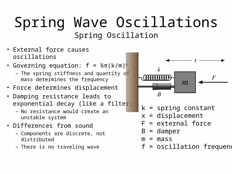
Rope Impulse Waves• A hand jerk is an impulse

– An impulse causes a wave to travel.– Speed of impulses determines frequency

• Rope stiffness determines wave velocity

• Reverse waves start at the fixed end– Resonates when waves correlate– Cancels when waves don’t correlate– Eventually a steady state is reached and we

perceive no motion (standing wave)– Boundary conditions model the interaction

• Sound differences– lateral verses transverse motion– Waves escape for non-stop sounds

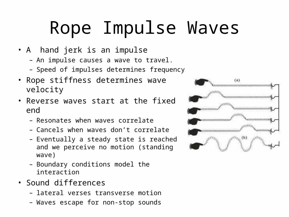
Acoustic Compression Waves

• Resistance– sources of energy loss– Ex: Vocal tract walls

• Impedence (Z)– Resistance to wave motion

• Capacitance – air resistance to

compression• Reflection

– Portion of waves that reflect back to the source

Compression and Rarefaction

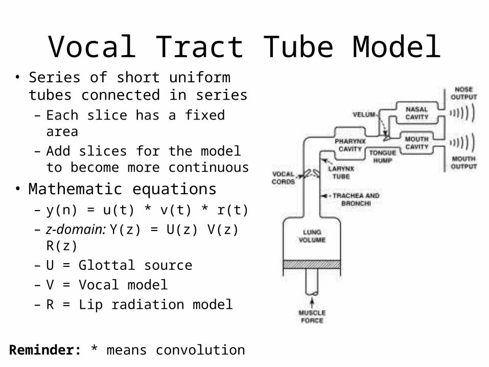
Vocal Tract Tube Model• Series of short uniform tubes

connected in series– Each slice has a fixed area– Add slices for the model to

become more continuous

• Mathematic equations– y(n) = u(t) * v(t) * r(t)– z-domain: Y(z) = U(z) V(z) R(z)– U = Glottal source– V = Vocal model– R = Lip radiation model

Reminder: * means convolution

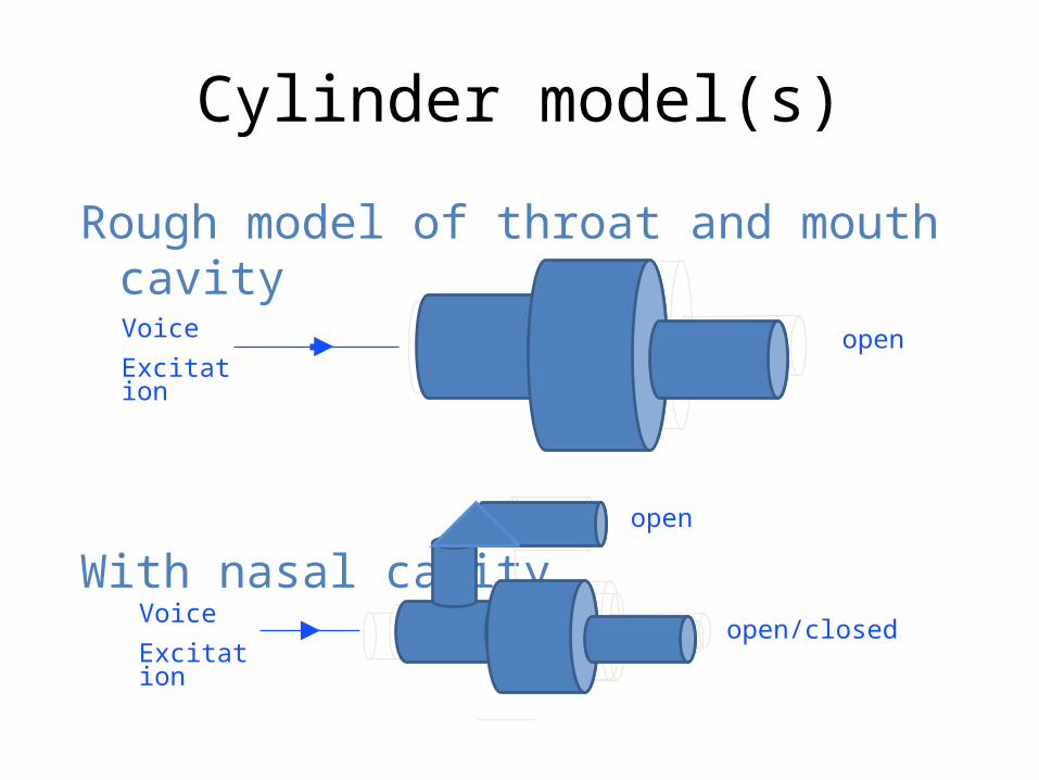
Cylinder model(s)

Rough model of throat and mouth cavity

With nasal cavity

Voice

Excitation

Voice

Excitation

open

open

open/closed

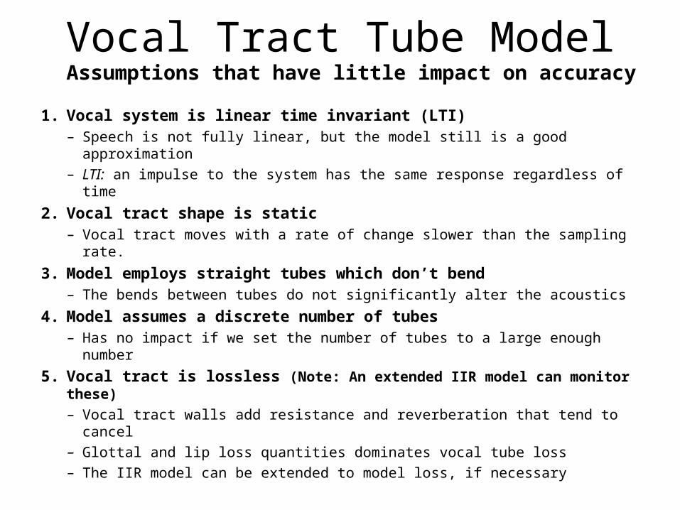
Vocal Tract Tube ModelAssumptions that have little impact on accuracy

1. Vocal system is linear time invariant (LTI)– Speech is not fully linear, but the model still is a good approximation– LTI: an impulse to the system has the same response regardless of time

2. Vocal tract shape is static– Vocal tract moves with a rate of change slower than the sampling rate.

3. Model employs straight tubes which don’t bend– The bends between tubes do not significantly alter the acoustics

4. Model assumes a discrete number of tubes– Has no impact if we set the number of tubes to a large enough number

5. Vocal tract is lossless (Note: An extended IIR model can monitor these)– Vocal tract walls add resistance and reverberation that tend to cancel– Glottal and lip loss quantities dominates vocal tube loss– The IIR model can be extended to model loss, if necessary

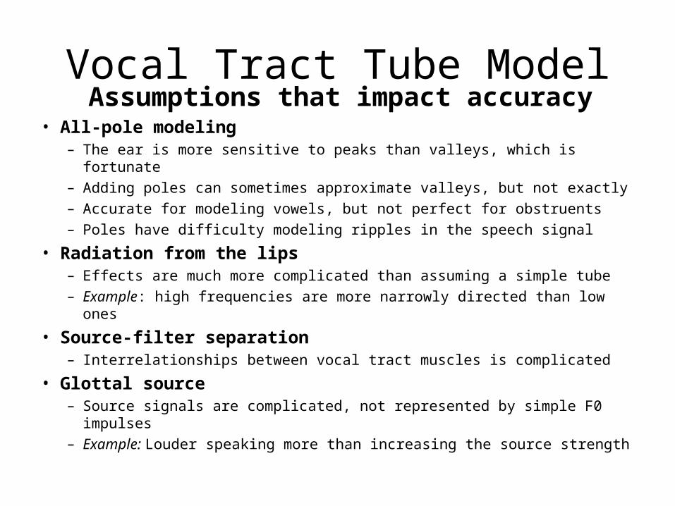
Vocal Tract Tube ModelAssumptions that impact accuracy

• All-pole modeling– The ear is more sensitive to peaks than valleys, which is fortunate– Adding poles can sometimes approximate valleys, but not exactly– Accurate for modeling vowels, but not perfect for obstruents– Poles have difficulty modeling ripples in the speech signal

• Radiation from the lips– Effects are much more complicated than assuming a simple tube– Example: high frequencies are more narrowly directed than low ones

• Source-filter separation– Interrelationships between vocal tract muscles is complicated

• Glottal source– Source signals are complicated, not represented by simple F0 impulses– Example: Louder speaking more than increasing the source strength

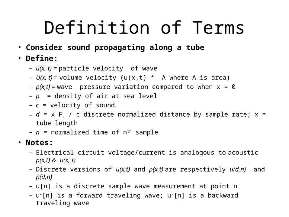
Definition of Terms• Consider sound propagating along a tube • Define:

– u(x, t) = particle velocity of wave– U(x, t) = volume velocity (u(x,t) * A where A is area)– p(x,t) = wave pressure variation compared to when x = 0– ρ = density of air at sea level– c = velocity of sound– d = x Fs / c discrete normalized distance by sample rate; x = tube length

– n = normalized time of nth sample

• Notes: – Electrical circuit voltage/current is analogous to acoustic p(x,t) & u(x, t)– Discrete versions of u(x,t) and p(x,t) are respectively u(d,n) and p(d,n)– u[n] is a discrete sample wave measurement at point n– u+[n] is a forward traveling wave; u-[n] is a backward traveling wave

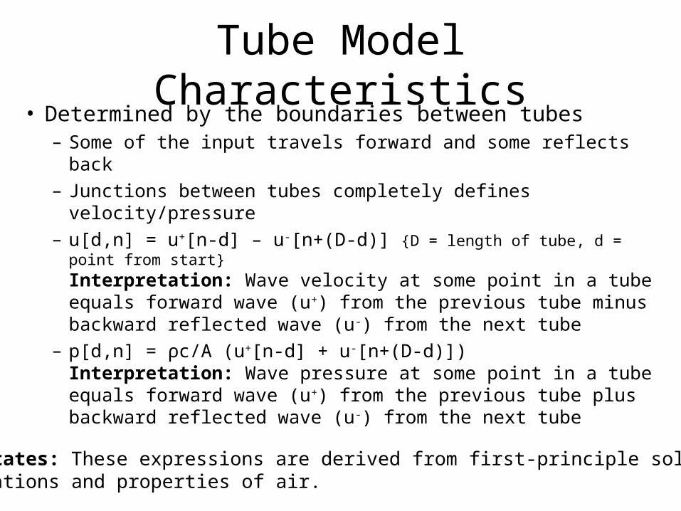
Tube Model Characteristics• Determined by the boundaries between tubes

– Some of the input travels forward and some reflects back– Junctions between tubes completely defines velocity/pressure– u[d,n] = u+[n-d] – u-[n+(D-d)] {D = length of tube, d = point from start}

Interpretation: Wave velocity at some point in a tube equals forward wave (u+) from the previous tube minus backward reflected wave (u-) from the next tube

– p[d,n] = ρc/A (u+[n-d] + u-[n+(D-d)])Interpretation: Wave pressure at some point in a tube equals forward wave (u+) from the previous tube plus backward reflected wave (u-) from the next tube

Author states: These expressions are derived from first-principle solution of wave equations and properties of air.

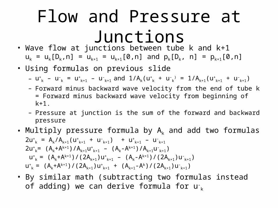
Flow and Pressure at Junctions• Wave flow at junctions between tube k and k+1

uk = uk[Dk,n] = uk+1 = uk+1[0,n] and pk[Dk, n] = pk+1[0,n]

• Using formulas on previous slide– u+

k – u-k = u+

k+1 – u-k+1

and 1/Ak(u+k + u-

k) = 1/Ak+1(u+

k+1 + u-k+1)

– Forward minus backward wave velocity from the end of tube k = Forward minus backward wave velocity from beginning of k+1.

– Pressure at junction is the sum of the forward and backward pressure

• Multiply pressure formula by Ak and add two formulas2u+

k = Ak/Ak+1(u+k+1 + u-

k+1) + u+k+1 – u-

k+1

2u+k= (Ak+Ak+1)/Ak+1u+

k+1 – (Ak-Ak+1)/Ak+1u-k+1)

u+k

= (Ak+Ak+1)/(2Ak+1)u+k+1 – (Ak-Ak+1)/(2Ak+1)u-

k+1)u+

k = (Ak+Ak+1)/(2Ak+1)u+

k+1 + (Ak+1-Ak)/(2Ak+1)u-k+1)

• By similar math (subtracting two formulas instead of adding) we can derive formula for u-

k

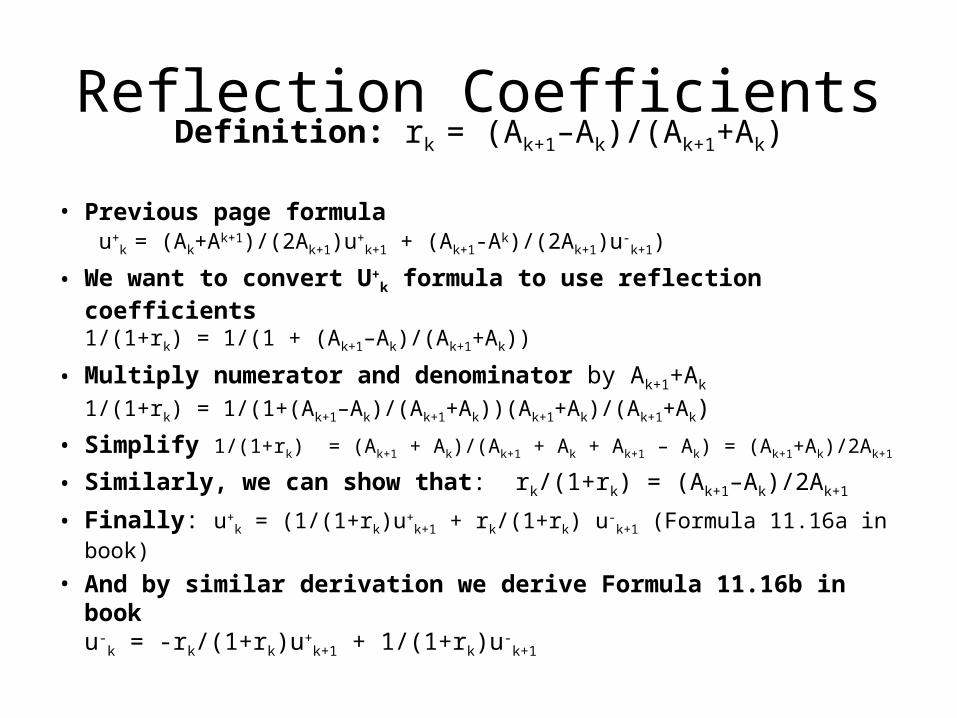
Reflection Coefficients

• Previous page formula u+

k = (Ak+Ak+1)/(2Ak+1)u+

k+1 + (Ak+1-Ak)/(2Ak+1)u-k+1)

• We want to convert U+k formula to use reflection coefficients

1/(1+rk) = 1/(1 + (Ak+1–Ak)/(Ak+1+Ak))

• Multiply numerator and denominator by Ak+1+Ak

1/(1+rk) = 1/(1+(Ak+1–Ak)/(Ak+1+Ak))(Ak+1+Ak)/(Ak+1+Ak)

• Simplify 1/(1+rk) = (Ak+1 + Ak)/(Ak+1 + Ak + Ak+1 – Ak) = (Ak+1+Ak)/2Ak+1

• Similarly, we can show that: rk/(1+rk) = (Ak+1–Ak)/2Ak+1

• Finally: u+k = (1/(1+rk)u+

k+1 + rk/(1+rk) u-k+1 (Formula 11.16a in book)

• And by similar derivation we derive Formula 11.16b in booku-

k = -rk/(1+rk)u+k+1 + 1/(1+rk)u-

k+1

Definition: rk = (Ak+1–Ak)/(Ak+1+Ak)

General Model• Wave at junction

u+k = (1/(1+rk)u+

k+1 + rk/(1+rk) u-k+1

u-k = -rk/(1+rk)u+

k+1 + 1/(1+rk)u-k+1

• Take Z transform of wave at junction

U+k(z) = (zD

k/(1+rk)U+k+1 + rkzD

k/(1+rk) U-k+1

U-k(z) = -rkz-D

k/(1+rk)U+k+1 + z-D

k/(1+rk)U-k+1

• Note– The Z exponent is positive for forward traveling waves and negative

for backward traveling waves. In one case the wave is sped up and in the other the wave is being delayed. It is like moving the imaginary axis of the Z plane left or right

– Assumptions: Reflection waves from the lips = 0 – All reflection back to the glottis is absorbed by the lungs

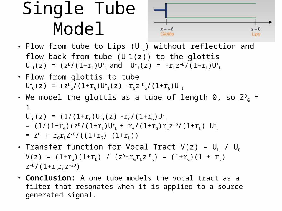
Single Tube Model

• Flow from tube to Lips (U+L) without reflection and flow back

from tube (U-1(z)) to the glottisU+

1(z) = (zD/(1+rL)U+L and U-

1(z) = -rLz-D/(1+rL)U+L

• Flow from glottis to tubeU+

G(z) = (zDG/(1+rG)U+

1(z) -rGz-DG/(1+rG)U-

1

• We model the glottis as a tube of length 0, so ZDG = 1

U+G(z) = (1/(1+rG)U+

1(z) -rG/(1+rG)U-1

= (1/(1+rG)(zD/(1+rL)U+L + rG/(1+rG)rLz-D/(1+rL) U+

L

= ZD + rGrLZ-D/((1+rG) (1+rL))

• Transfer function for Vocal Tract V(z) = UL / UG

V(z) = (1+rG)(1+rL) / (zD+rGrLz-Dk) = (1+rG)(1 + rL) z-D/(1+rGrLz-2D)

• Conclusion: A one tube models the vocal tract as a filter that resonates when it is applied to a source generated signal.

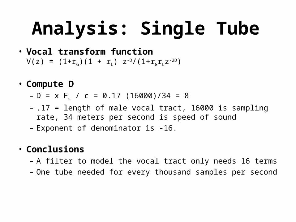
Analysis: Single Tube• Vocal transform function

V(z) = (1+rG)(1 + rL) z-D/(1+rGrLz-2D)

• Compute D– D = x Fs / c = 0.17 (16000)/34 = 8

– .17 = length of male vocal tract, 16000 is sampling rate, 34 meters per second is speed of sound

– Exponent of denominator is -16.

• Conclusions– A filter to model the vocal tract only needs 16 terms– One tube needed for every thousand samples per second

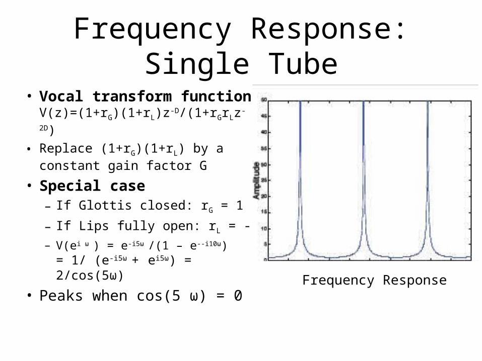
Frequency Response: Single Tube

• Vocal transform functionV(z)=(1+rG)(1+rL)z-D/(1+rGrLz-2D)

• Replace (1+rG)(1+rL) by a constant gain factor G

• Special case– If Glottis closed: rG = 1

– If Lips fully open: rL = -1– V(ei ω ) = e-i5ω /(1 – e--i10ω)

= 1/ (e-i5ω + ei5ω) = 2/cos(5ω)

• Peaks when cos(5 ω) = 0

Frequency Response

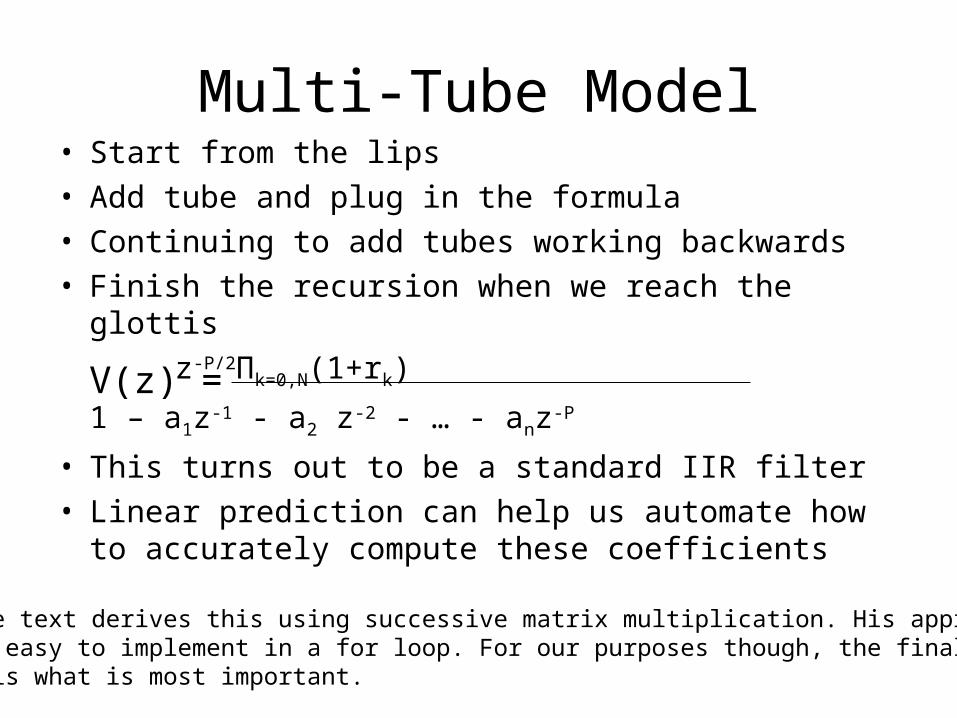
Multi-Tube Model• Start from the lips• Add tube and plug in the formula• Continuing to add tubes working backwards• Finish the recursion when we reach the glottis

z-P/2Πk=0,N(1+rk)

1 – a1z-1 - a2 z-2 - … - anz-P

• This turns out to be a standard IIR filter• Linear prediction can help us automate how to

accurately compute these coefficients

V(z) =

Note: The text derives this using successive matrix multiplication. His approach is fine and easy to implement in a for loop. For our purposes though, the final formula is what is most important.

The All Pole Model• Using a Gain factor, G, an IIR filter can model the vocal tract• The model needs a pole for each 1k of the sample rate

– A multi-pole model results in more non-zero filter coefficients– Adding extra poles will not increase accuracy– Factoring a filter’s polynomial roughly estimates the formants– Actual pole locations don’t correspond to specific tubes. They

result from all of the interactions between the tubes– Adding zeros to the model can account for anti resonances

• CELP (Code Excited Linear Prediction) – memorizes banks of vocal tract IIR filters for signal compression– The residue is the difference between the actual and modeled signal– Idea: It takes less bits to save the residue than the original signal

Radiation• A speech signal travel some distance before being heard

• There is impedance at the lips that alters the signal to somewhat increases the high frequency amplitudes

• This can be modeled by an additional filter, but an accurate model is quite complicated

• An adequate model– Transfer function: R(z) = P(z)/UL(z)

– Pressure (P) = Output (UL) times impedance (R)

– Typical implementation: R(z) = 1 – αz-1 where .95<α<.98– Result: approximate 6dB boost per octave

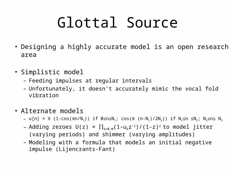
Glottal Source

• Designing a highly accurate model is an open research area

• Simplistic model– Feeding impulses at regular intervals– Unfortunately, it doesn’t accurately mimic the vocal fold vibration

• Alternate models– u[n] = ½ (1-cos(πn/N1)) if 0≤n≤N1; cos(π (n-N1)/2N2)) if N1≤n ≤N2; N2≤n≤ N3

– Adding zeroes U(z) = ∏k=0,M(1-ukz-1)/(1-z)2 to model jitter (varying periods) and shimmer (varying amplitudes)

– Modeling with a formula that models an initial negative impulse (Lijencrants-Fant)

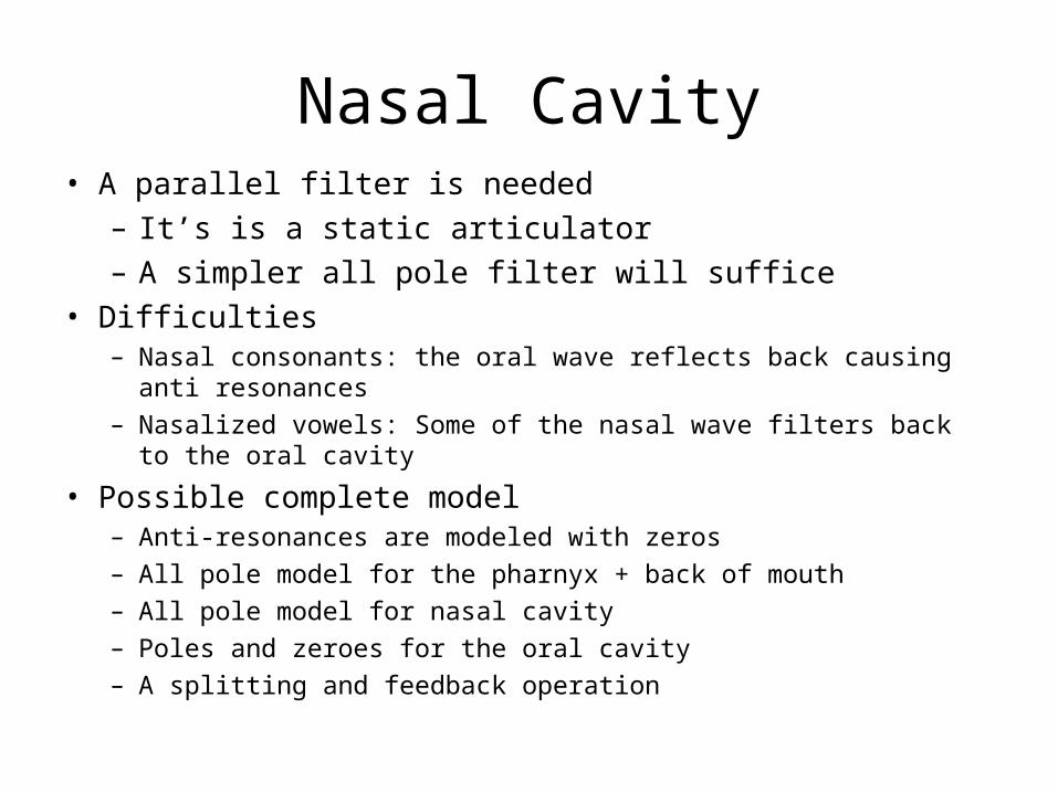
Nasal Cavity• A parallel filter is needed

– It’s is a static articulator– A simpler all pole filter will suffice

• Difficulties– Nasal consonants: the oral wave reflects back causing anti resonances– Nasalized vowels: Some of the nasal wave filters back to the oral cavity

• Possible complete model– Anti-resonances are modeled with zeros– All pole model for the pharnyx + back of mouth– All pole model for nasal cavity– Poles and zeroes for the oral cavity– A splitting and feedback operation

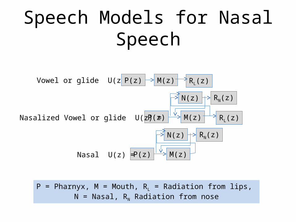
Speech Models for Nasal Speech

Vowel or glide U(z) = P(z) M(z) RL(z)

P(z) M(z) RL(z)Nasalized Vowel or glide U(z) =

P = Pharnyx, M = Mouth, RL = Radiation from lips, N = Nasal, RN Radiation from nose

N(z) RN(z)

P(z) M(z)Nasal U(z) =

N(z) RN(z)

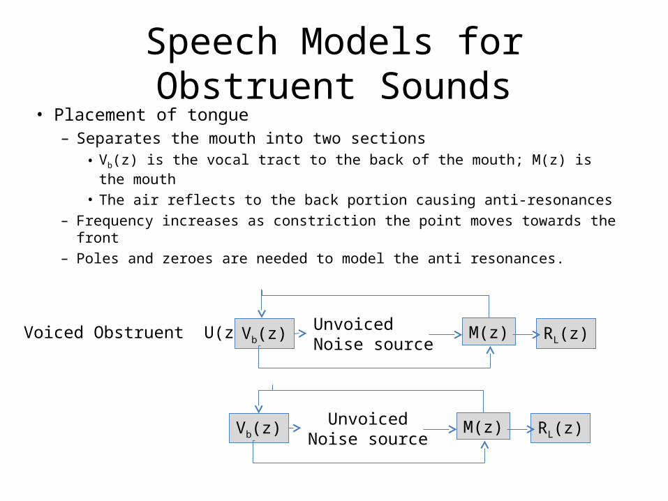
Speech Models for Obstruent Sounds• Placement of tongue

– Separates the mouth into two sections • Vb(z) is the vocal tract to the back of the mouth; M(z) is the mouth

• The air reflects to the back portion causing anti-resonances– Frequency increases as constriction the point moves towards the front– Poles and zeroes are needed to model the anti resonances.

Voiced Obstruent U(z) = Vb(z) M(z) RL(z)UnvoicedNoise source

Vb(z) M(z) RL(z)UnvoicedNoise source