The Cross-Entropy Method for Optimization

Zdravko I. Botev, Department of Computer Science and Operations Research,Universite de Montreal, Montreal Quebec H3C 3J7, Canada.botev@iro.umontreal.ca

Dirk P. Kroese, School of Mathematics and Physics, The University of Queens-land, Brisbane 4072, Australia.kroese@maths.uq.edu.au.

Reuven Y. Rubinstein, Faculty of Industrial Engineering and Management,Technion, Haifa, Israel.ierrr01@ie.technion.ac.il

Pierre L’Ecuyer, Department of Computer Science and Operations Research,Universite de Montreal, Montreal Quebec H3C 3J7, Canada.lecuyer@iro.umontreal.ca

Abstract

The cross-entropy method is a versatile heuristic tool for solving difficult estima-tion and optimization problems, based on Kullback–Leibler (or cross-entropy)minimization. As an optimization method it unifies many existing population-based optimization heuristics. In this chapter we show how the cross-entropymethod can be applied to a diverse range of combinatorial, continuous, andnoisy optimization problems.

1 Introduction

The cross-entropy (CE) method was proposed by Rubinstein (1997) as an adap-tive importance sampling procedure for the estimation of rare-event probabili-ties, that uses the cross-entropy or Kullback–Leibler divergence as a measure ofcloseness between two sampling distributions. Subsequent work by Rubinstein(1999; 2001) has shown that many optimization problems can be translated intoa rare-event estimation problem. As a result, adaptive importance samplingmethods such as the CE method can be utilized as randomized algorithms foroptimization. The gist of the idea is that the probability of locating an optimalor near optimal solution using naive random search is a rare-event probability.The cross-entropy method can be used to gradually change the sampling dis-tribution of the random search so that the rare-event is more likely to occur.For this purpose, using the CE distance, the method estimates a sequence ofsampling distributions that converges to a distribution with probability massconcentrated in a region of near-optimal solutions.

To date, the CE method has been successfully applied to mixed integernonlinear programming (Kothari and Kroese 2009); continuous optimal con-trol problems (Sani 2009, Sani and Kroese 2008); continuous multi-extremaloptimization (Kroese et al. 2006); multidimensional independent componentanalysis (Szabo et al. 2006); optimal policy search (Busoniu et al. 2010); clus-tering (Botev and Kroese 2004, Kroese et al. 2007b, Boubezoula et al. 2008);

1

signal detection (Liu et al. 2004); DNA sequence alignment (Keith and Kroese2002, Pihur et al. 2007); noisy optimization problems such as optimal bufferallocation (Alon et al. 2005); resource allocation in stochastic systems (Co-hen et al. 2007); network reliability optimization (Kroese et al. 2007a); vehiclerouting optimization with stochastic demands (Chepuri and Homem-de-Mello2005); power system combinatorial optimization problems (Ernst et al. 2007);and neural and reinforcement learning (Lorincza et al. 2008, Menache et al.2005, Unveren and Acan 2007, Wu and Fyfe 2008).

A tutorial on the CE method is given in de Boer et al. (2005). A com-prehensive treatment can be found in Rubinstein and Kroese (2004); see alsoRubinstein and Kroese (2007; Chapter 8). The CE method homepage is www.

cemethod.org.

2 From Estimation to Optimization

The CE method can be applied to two types of problems:

1. Estimation: Estimate ` = E[H(X)], where X is a random object takingvalues in some set X and H is a function on X . An important specialcase is the estimation of a probability ` = P(S(X) > γ), where S isanother function on X .

2. Optimization: Optimize (that is, maximize or minimize) a given objec-tive function S(x) over all x ∈ X . S can be either a known or a noisyfunction. In the latter case the objective function needs to be estimated,e.g., via simulation.

In this section we review the CE method as an adaptive importance samplingmethod for rare-event probability estimation, and in the next section we showhow the CE estimation algorithm leads naturally to an optimization heuristic.

Cross-Entropy for Rare-event Probability Estimation

Consider the estimation of the probability

` = P(S(X) > γ) = E[I{S(X)>γ}] =

∫I{S(x)>γ} f(x;u) dx , (1)

where S is a real-valued function, γ is a threshold or level parameter, andthe random variable X has probability density function (pdf) f(·;u), which isparameterized by a finite-dimensional real vector u. We write X ∼ f(·;u). IfX is a discrete variable, simply replace the integral in (1) by a sum. We areinterested in the case where ` is a rare-event probability ; that is, a very smallprobability, say, less than 10−4. Let g be another pdf such that g(x) = 0 ⇒H(x) f(x;u) = 0 for every x. Using the pdf g we can represent ` as

` =

∫f(x;u) I{S(x)>γ}

g(x)g(x) dx = E

[f(X;u) I{S(X)>γ}

g(X)

], X ∼ g . (2)

2

Consequently, if X1, . . . ,XN are independent random vectors with pdf g, writ-ten as X1, . . . ,XN ∼iid g, then

=1

N

N∑

k=1

I{S(Xk)>γ}f(Xk;u)

g(Xk)(3)

is an unbiased estimator of `: a so-called importance sampling estimator. It iswell known (see, for example, (Rubinstein and Kroese 2007; Page 132)) thatthe optimal importance sampling pdf (that is, the pdf g∗ for which the varianceof is minimal) is the density of X conditional on the event S(X) > γ; that is,

g∗(x) =f(x;u) I{S(x)>γ}

`. (4)

The idea of the CE method is to choose the importance sampling pdf g fromwithin the parametric class of pdfs {f(·;v), v ∈ V} such that the Kullback–Leibler divergence between the optimal importance sampling pdf g∗ and g isminimal. The Kullback–Leibler divergence between g∗ and g is given by

D(g∗, g) =

∫g∗(x) ln

g∗(x)

g(x)dx = E

[ln

g∗(X)

g(X)

], X ∼ g∗ . (5)

The CE minimization procedure then reduces to finding an optimal referenceparameter vector, v∗ say, by cross-entropy minimization:

v∗ = argminv

D(g∗, f(·;v))

= argmaxv

EuI{S(X)>γ} ln f(X;v)

= argmaxv

EwI{S(X)>γ} ln f(X;v)f(X;u)

f(X;w), (6)

where w is any reference parameter and the subscript in the expectation op-erator indicates the density of X. This v∗ can be estimated via the stochasticcounterpart of (6):

v = argmaxv

1

N

N∑

k=1

I{S(X)>γ}f(Xk;u)

f(Xk;w)ln f(Xk;v) , (7)

where X1, . . . ,XN ∼iid f(·;w). The optimal parameter v in (7) can often beobtained in explicit form, in particular when the class of sampling distributionsforms an exponential family (Rubinstein and Kroese 2007; Pages 319–320). In-deed, analytical updating formulas can be found whenever explicit expressionsfor the maximal likelihood estimators of the parameters can be found (de Boeret al. 2005; Page 36).

A complication in solving (7) is that for a rare-event probability ` most orall of the indicators I{S(X)>γ} in (7) are zero, and the maximization problembecomes useless. In that case a multi-level CE procedure is used, where asequence of reference parameters {vt} and levels {γt} is constructed with the

3

goal that the former converges to v∗ and the latter to γ. At each iteration twe simulate N independent random variables X1, . . . ,XN from the currentlyestimated importance sampling density f(·; vt−1) and let γt be the (1 − %)-quantile of the performance values S(X1), . . . , S(XN ), where % is a user specifiedparameter called the rarity parameter. We then update the value of vt−1 tovt, where vt is calculated using likelihood maximization (or equivalently crossentropy minimization) based on the N e = d%Ne random variables for whichS(Xi) > γt.

This leads to the following algorithm (Rubinstein and Kroese 2007; Page238).

Algorithm 2.1 (CE Algorithm for Rare-Event Estimation) Given the sam-ple size N and the parameter %, execute the following steps.

1. Define v0 = u. Let N e = d%Ne. Set t = 1 (iteration counter).

2. Generate X1, . . . ,XN ∼iid f(·; vt−1). Calculate Si = S(Xi) for all i, andorder these from smallest to largest: S(1) 6 . . . 6 S(N). Let γt be thesample (1 − %)-quantile of performances; that is, γt = S(N−Ne+1). Ifγt > γ, reset γt to γ.

3. Use the same sample X1, . . . ,XN to solve the stochastic program (7),with w = vt−1. Denote the solution by vt.

4. If γt < γ, set t = t + 1 and reiterate from Step 2; otherwise, proceed withStep 5.

5. Let T = t be the final iteration counter. Generate X1, . . . ,XN1 ∼iid

f(·; vT ) and estimate ` via importance sampling, as in (3) with u = vT .

We now show how this estimation algorithm leads naturally to a simple opti-mization heuristic.

Cross-Entropy Method for Optimization

To see how Algorithm 2.1 can be used for optimization purposes, suppose thatthe goal is to find the maximum of S(x) over a given set X . Assume, forsimplicity, that there is only one maximizer x∗. Denote the maximum by γ∗,so that

S(x∗) = γ∗ = maxx∈X

S(x) . (8)

We can now associate with the above optimization problem the estimationof the probability ` = P(S(X) > γ), where X has some probability densityf(x;u) on X (for example corresponding to the uniform distribution on X )and γ is close to the unknown γ∗. Typically, ` is a rare-event probability, andthe multi-level CE approach of Algorithm 2.1 can be used to find an importancesampling distribution that concentrates all its mass in a neighborhood of thepoint x∗. Sampling from such a distribution thus produces optimal or near-optimal states. Note that, in contrast to the rare-event simulation setting,

4

the final level γ = γ∗ is generally not known in advance, but the CE methodfor optimization produces a sequence of levels {γt} and reference parameters{vt} such that ideally the former tends to the optimal γ∗ and the latter to theoptimal reference vector v∗ corresponding to the point mass at x∗; see, e.g.,(Rubinstein and Kroese 2007; Page 251).

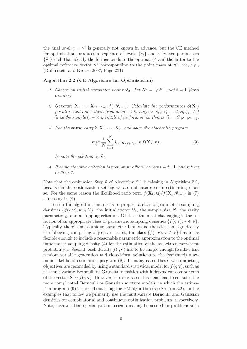
Algorithm 2.2 (CE Algorithm for Optimization)

1. Choose an initial parameter vector v0. Let N e = d%Ne. Set t = 1 (levelcounter).

2. Generate X1, . . . ,XN ∼iid f(·; vt−1). Calculate the performances S(Xi)for all i, and order them from smallest to largest: S(1) 6 . . . 6 S(N). Letγt be the sample (1−%)-quantile of performances; that is, γt = S(N−Ne+1).

3. Use the same sample X1, . . . ,XN and solve the stochastic program

maxv

1

N

N∑

k=1

I{S(Xk)>bγt} ln f(Xk;v) . (9)

Denote the solution by vt.

4. If some stopping criterion is met, stop; otherwise, set t = t+1, and returnto Step 2.

Note that the estimation Step 5 of Algorithm 2.1 is missing in Algorithm 2.2,because in the optimization setting we are not interested in estimating ` perse. For the same reason the likelihood ratio term f(Xk;u)/f(Xk; vt−1) in (7)is missing in (9).

To run the algorithm one needs to propose a class of parametric samplingdensities {f(·;v),v ∈ V}, the initial vector v0, the sample size N , the rarityparameter %, and a stopping criterion. Of these the most challenging is the se-lection of an appropriate class of parametric sampling densities {f(·;v),v ∈ V}.Typically, there is not a unique parametric family and the selection is guided bythe following competing objectives. First, the class {f(·;v),v ∈ V} has to beflexible enough to include a reasonable parametric approximation to the optimalimportance sampling density (4) for the estimation of the associated rare-eventprobability `. Second, each density f(·;v) has to be simple enough to allow fastrandom variable generation and closed-form solutions to the (weighted) max-imum likelihood estimation program (9). In many cases these two competingobjectives are reconciled by using a standard statistical model for f(·;v), such asthe multivariate Bernoulli or Gaussian densities with independent componentsof the vector X ∼ f(·;v). However, in some cases it is beneficial to consider themore complicated Bernoulli or Gaussian mixture models, in which the estima-tion program (9) is carried out using the EM algorithm (see Section 3.2). In theexamples that follow we primarily use the multivariate Bernoulli and Gaussiandensities for combinatorial and continuous optimization problems, respectively.Note, however, that special parameterizations may be needed for problems such

5

as the traveling salesman problem, where the optimization is carried out over aset of possible permutations; see Rubinstein and Kroese (2004) for more details.

In applying Algorithm 2.2, the following smoothed updating has proven use-ful. Let vt be the solution to (9) and 0 6 α 6 1 be a smoothing parameter,then for the next iteration we take the parameter vector

vt = α vt + (1− α) vt−1 . (10)

Other modifications can be found in Kroese et al. (2006), Rubinstein and Kroese(2004), and Rubinstein and Kroese (2007). The effect that smoothing has onconvergence is discussed in detail in Costa et al. (2007). In particular, it is shownthat for discrete binary optimization problems with non-constant smoothingvt = αt vt + (1 − αt) vt−1, αt ∈ [0, 1] the optimal solution is generated withprobability 1 if the smoothing sequence {αt} satisfies:

∞∑

t=1

t∏

k=1

(1− αk)n =∞ ,

where n is the length of the binary vector x. Other convergence results can befound in Rubinstein and Kroese (2004) and Margolin (2005). Finally, significantspeed up can be achieved by using a parallel implementation of CE (Evans et al.2007).

3 Applications to Combinatorial Optimization

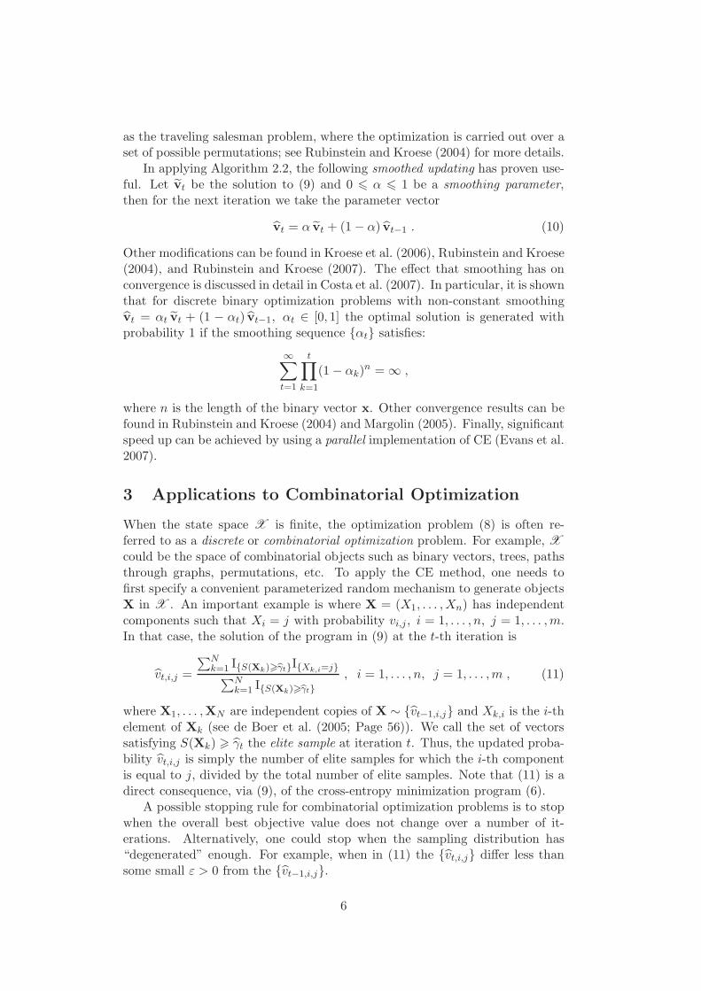
When the state space X is finite, the optimization problem (8) is often re-ferred to as a discrete or combinatorial optimization problem. For example, X

could be the space of combinatorial objects such as binary vectors, trees, pathsthrough graphs, permutations, etc. To apply the CE method, one needs tofirst specify a convenient parameterized random mechanism to generate objectsX in X . An important example is where X = (X1, . . . ,Xn) has independentcomponents such that Xi = j with probability vi,j , i = 1, . . . , n, j = 1, . . . ,m.In that case, the solution of the program in (9) at the t-th iteration is

vt,i,j =

∑Nk=1 I{S(Xk)>bγt}I{Xk,i=j}∑N

k=1 I{S(Xk)>bγt}

, i = 1, . . . , n, j = 1, . . . ,m , (11)

where X1, . . . ,XN are independent copies of X ∼ {vt−1,i,j} and Xk,i is the i-thelement of Xk (see de Boer et al. (2005; Page 56)). We call the set of vectorssatisfying S(Xk) > γt the elite sample at iteration t. Thus, the updated proba-bility vt,i,j is simply the number of elite samples for which the i-th componentis equal to j, divided by the total number of elite samples. Note that (11) is adirect consequence, via (9), of the cross-entropy minimization program (6).

A possible stopping rule for combinatorial optimization problems is to stopwhen the overall best objective value does not change over a number of it-erations. Alternatively, one could stop when the sampling distribution has“degenerated” enough. For example, when in (11) the {vt,i,j} differ less thansome small ε > 0 from the {vt−1,i,j}.

6

3.1 Knapsack Packing Problem

A well-known NP-complete combinatorial optimization problem is the 0-1 knap-sack problem (Kellerer et al. 2004) defined as:

maxx

n∑

j=1

pjxj, xj ∈ {0, 1}, j = 1, . . . , n ,

subject to :n∑

j=1

wi,jxj 6 ci, i = 1, . . . ,m .

(12)

Here {pj} and {wi,j} are positive weights, {ci} are positive cost parameters,and x = (x1, . . . , xn). In order to define a single objective function, we adoptthe penalty function approach and define

S(x)def= β

m∑

i=1

I{Pj wi,j xj>ci} +

n∑

j=1

pj xj ,

where β = −∑nj=1 pj. In this way, S(x) 6 0 if one of the inequality constraints

is not satisfied and S(x) =∑n

j=1 pj xj is all of the constraints are satisfied.As a particular example, consider the Sento1.dat knapsack problem given inthe appendix of Senju and Toyoda (1968). The problem has 30 constraintsand 60 variables. Since the solution vector x is binary, a simple choice for thesampling density in Step 2 of Algorithm 2.2 is the multivariate Bernoulli densityf(x;v) =

∏nj=1 v

xj

j (1 − vj)1−xj . We apply Algorithm 2.2 to this particular

problem with N = 103 and N e = 20, v0 = (1/2, . . . , 1/2). Note that we do notuse any smoothing for vt (that is, α = 1 in (10)) and the solution vt of (9) ateach iteration is given by

vt,j =

∑Nk=1 I{bS(Xk)>bγt}

Xk,j∑N

k=1 I{bS(Xk)>bγt}

, j = 1, . . . , n , (13)

where Xk,j is the j-th component of the k-th random binary vector X. In Step 4of Algorithm 2.2 we stop the algorithm if dt = max16j6n{min{vt,j , 1− vt,j}} 6

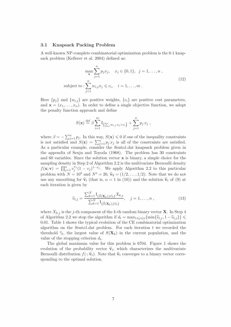
0.01. Table 1 shows the typical evolution of the CE combinatorial optimizationalgorithm on the Sento1.dat problem. For each iteration t we recorded thethreshold γt, the largest value of S(Xk) in the current population, and thevalue of the stopping criterion dt.

The global maximum value for this problem is 6704. Figure 1 shows theevolution of the probability vector vt, which characterizes the multivariateBernoulli distribution f(·; vt). Note that vt converges to a binary vector corre-sponding to the optimal solution.

7

Table 1: Typical evolution of the CE method on the knapsack problem. Thelast column shows the stopping value dt = max16j6n{min{vt,j , 1 − vt,j}} foreach t.

t γt best score dt

1 −192450 −45420 0.4952 −119180 1056 0.4553 −48958 1877 0.3954 −8953 3331 0.345 1186 3479 0.4156 2039.5 4093 0.4557 2836.5 4902 0.4358 3791 5634 0.485

t γt best score dt

9 4410 5920 0.4610 5063.5 6246 0.4611 5561 6639 0.45212 5994.5 6704 0.4713 6465.5 6704 0.4614 6626 6704 0.35515 6677 6704 0.34616 6704 6704 0

1 4 7 10 13 16 19 22 25 28 31 34 37 40 43 46 49 52 55 580

0.5

1

1 4 7 10 13 16 19 22 25 28 31 34 37 40 43 46 49 52 55 580

0.5

1

1 4 7 10 13 16 19 22 25 28 31 34 37 40 43 46 49 52 55 580

0.5

1

1 4 7 10 13 16 19 22 25 28 31 34 37 40 43 46 49 52 55 580

0.5

1

1 4 7 10 13 16 19 22 25 28 31 34 37 40 43 46 49 52 55 580

0.5

1

1 4 7 10 13 16 19 22 25 28 31 34 37 40 43 46 49 52 55 580

0.5

1

i

t = 13

t = 10

t = 7

t = 4

t = 1

t = 16

Figure 1: The evolution of the probability vector vt.

8

3.2 Boolean Satisfiability Problem

Let x = (x1, . . . , xn) be a binary vector and suppose c1(x), . . . , cm(x) are mfunctions, called clause functions, such that ci : {0, 1}n → {0, 1}. For givenclauses, the objective is to find

x∗ = argmaxx∈{0,1}n

m∏

i=1

ci(x) . (14)

That is, to find a vector x∗ satisfying all clauses simultaneously. This Booleansatisfiability (SAT) problem (Gu et al. 1997) is of importance in computerscience and operations research, because any NP-complete problem, such as thetraveling salesman problem, can be translated into a SAT problem in polynomialtime.

We now show how one can apply Algorithm 2.2 to the SAT problem. First,note that the function

∏mi=1 ci(x) in (14) takes on only the values 0 or 1, and

is thus not suitable for the level approach in the CE method. A more suitableand equivalent formulation is:

x∗ = argmaxx∈{0,1}n

S(x)def= argmax

x∈{0,1}n

m∑

i=1

ci(x) , (15)

where the function S : {0, 1}n → {1, . . . ,m}. In this way, the function S can beused to measure the distance from our goal by indicating the number of satisfiedclauses (as opposed to simply indicating whether all clauses are satisfied or not).As a specific example we consider the SAT instance uf75-01 from Hoos andStutzle (2000).

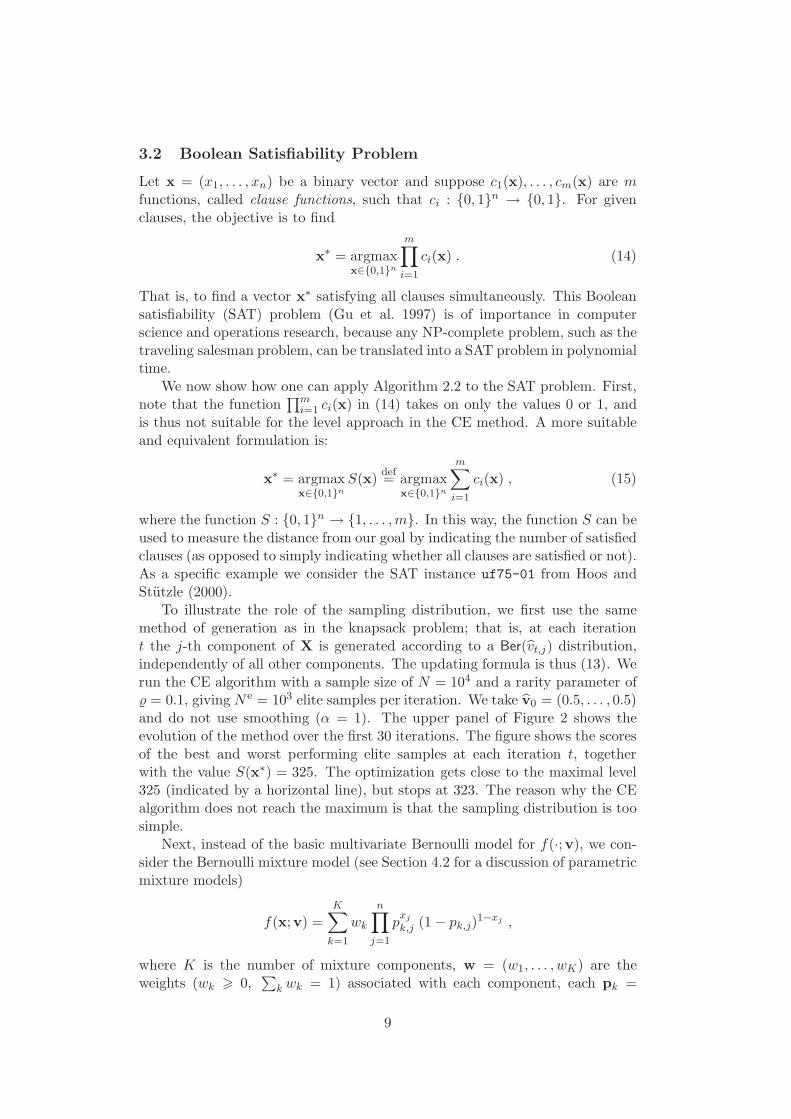
To illustrate the role of the sampling distribution, we first use the samemethod of generation as in the knapsack problem; that is, at each iterationt the j-th component of X is generated according to a Ber(vt,j) distribution,independently of all other components. The updating formula is thus (13). Werun the CE algorithm with a sample size of N = 104 and a rarity parameter of% = 0.1, giving N e = 103 elite samples per iteration. We take v0 = (0.5, . . . , 0.5)and do not use smoothing (α = 1). The upper panel of Figure 2 shows theevolution of the method over the first 30 iterations. The figure shows the scoresof the best and worst performing elite samples at each iteration t, togetherwith the value S(x∗) = 325. The optimization gets close to the maximal level325 (indicated by a horizontal line), but stops at 323. The reason why the CEalgorithm does not reach the maximum is that the sampling distribution is toosimple.

Next, instead of the basic multivariate Bernoulli model for f(·;v), we con-sider the Bernoulli mixture model (see Section 4.2 for a discussion of parametricmixture models)

f(x;v) =K∑

k=1

wk

n∏

j=1

pxj

k,j (1− pk,j)1−xj ,

where K is the number of mixture components, w = (w1, . . . , wK) are theweights (wk > 0,

∑k wk = 1) associated with each component, each pk =

9

(pk,1, . . . , pk,n) is a vector of probabilities, and v = (w,p1, . . . ,pK) collects allthe unknown parameters (we assume that K is given). The greater flexibilityin the parametric model comes at a cost — the maximum likelihood program(9) in Step 3 of Algorithm 2.2 no longer has a simple closed form solution.Nevertheless, an approximate solution of (9) can be obtained using the EMalgorithm of Dempster et al. (1977), where the initial starting point for theEM routine is chosen at random from the elite vectors. The lower panel ofFigure 2 shows the evolution of this CE algorithm using K = 6 componentsfor the Bernoulli mixture density and the same algorithmic parameters (N =104, % = 0.1, α = 1, v0 = (0.5, . . . , 0.5)). With this setup the algorithm quicklyreaches the desired level of 325, justifying the extra computational cost of fittinga parametric mixture model via the EM algorithm.

0 5 10 15 20 25 30290

300

310

320

330

t

S(x

)

0 5 10 15 20 25 30290

300

310

320

330

t

S(x

)

S(x∗) = 325

S(x∗) = 325

γt

γt

maxk S(Xk)maxk S(Xk)

maxk S(Xk)

Figure 2: Evolution of the CE algorithm on the uf75-01 SAT instance. Theupper panel corresponds to the case where f(x;v) is a multivariate Bernoullidensity and the lower panel corresponds to the case where f(x;v) is Bernoullimixture model with K = 6 components. Both panels show the best score,maxk S(Xk), and γt for each iteration t.

3.3 Network Planning Problem

An important integer optimization problem is the Network Planning Problem(NPP). Here a network is represented as an undirected graph with edges (links)that may fail with a given probability. The objective of the NPP is to optimallypurchase a collection of edges, subject to a fixed budget, so as to maximize thenetwork reliability — defined as the probability that all nodes in a given set of

10

nodes are connected by functioning edges. Each edge comes with a pre-specifiedcost and reliability (probability that it works). The NPP has applications inengineering (Wang et al. 2009), telecommunications, transportation, energysupply systems (de Silva et al. 2010, Kothari and Kroese 2009), computer andsocial networking (Hintsanen et al. 2010). The difficulty in solving this problemderives from the following aspects of the optimization.

1. Typically the computation of the reliability of large networks is a diffi-cult #P-complete computational problem, which either requires MonteCarlo simulation or sharp bounds on the reliability (Rubino 1998, Wonand Karray 2010). In the Monte Carlo case the NPP becomes a noisyoptimization problem, that is, the objective function values are estimatedfrom simulation.

2. For highly reliable networks, the network reliability is a rare-event proba-bility. In such cases Crude Monte Carlo simulation is impractical and onehas to resort to sophisticated rare-event probability estimation methods(Rubino and Tuffin 2009).

3. Even if the reliability could somehow be computed easily, thus dispensingwith the problems above, the NPP remains an NP-hard 0–1 knapsackoptimization problem with a nonlinear objective function. In response tothis, various optimization heuristics have been developed, such as sim-ulated annealing (Cancela and Urquhart 1995) and genetic algorithms(Dengiz et al. 1997, Reichelt et al. 2007).

4. Finally, the problem is constrained and for most optimization heuristicslike the simulated annealing and genetic algorithms, the penalty functionapproach is inefficient.

Here we apply the CE method to tackle all of the above problems simultane-ously. We now explain the implementation and mathematical details, largelyfollowing Kroese et al. (2007a).

Let G(V ,E ,K ) be an undirected graph, where V = {1, . . . , v} is the setof v nodes (vertices), E = {1, . . . , n} is the set of n edges, and K ⊆ V with|K | > 2 is the set of terminal nodes. Sometimes we may refer to an edge byspecifying the pair of nodes it connects, and write

E = {(vi, vj), . . . , (vk, vl)}, vi, vj , vk, vl ∈ V .

For example, in Figure 3 the edge set is given by

E = {(1, 2), (1, 3), (1, 6), (2, 3), (2, 4), (3, 4), (3, 6), (4, 5), (5, 6)} ,

and the set of terminal nodes is {2, 5}. For each e = 1, . . . , n let Be ∼ Ber(pe)be a Bernoulli random variable with success probability pe indicating whetherthe e-th link is operational. In other words, the event {Be = 1} correspondsto edge e being operational and the event {Be = 0} corresponds to the edgebeing nonoperational. It follows that each of the 2n states of the network canbe represented by a binary vector B = (B1, . . . , Bn). For example, the state of

11

Figure 3: A reliability network with 6 nodes and 9 edges or links. The networkworks if the two terminal nodes (filled circles) are connected by functioninglinks. Failed links are indicated by dashed lines.

the network on Figure 3 can be represented as B = (0, 0, 1, 1, 1, 1, 1, 1, 0). LetE [B] denote the set of operational edges corresponding to B. For example, theset of operational edges on Figure 3 is

E [B] = {(1, 6), (2, 3), (2, 4), (3, 4), (3, 6), (4, 5)} ≡ {3, 4, 5, 6, 7, 8} .

The size of the set of edges E [B] is |E [B]| = B1 + · · ·+Bn. The reliability of thenetwork is the probability that all of the nodes in K are connected by the setE [B] of operational edges. For a given set of edges E we define the structurefunction Φ as

Φ[E ] =

{1 if E contains a path connecting the nodes in K

0 if E does not contain a path connecting the nodes in K .

We can write the reliability of the network as

r =∑

b

Φ(E [b])

n∏

e=1

pbee (1− pe)

1−be = EΦ(E [B]) ,

where Be ∼ Ber(pe), independently for all e = 1, . . . , n. Denote by x =(x1, . . . , xn) the purchase vector with (e = 1, . . . , n)

xe =

{1 if link e is purchased

0 if link e is not purchased.

Let us denote by c = (c1, . . . , cn) the vector of link costs. Define

B(x) = (B1x1, . . . , Bnxn)

S(x) = EΦ(E [B(x)]) ,

12

where S(x) is the reliability for a given purchase vector x. Then, the NPP canbe written as:

maxx

S(x)

subject to:∑

e

xece 6 Cmax ,(16)

where Cmax is the available budget. We next address the problem of estimatingS(x) for highly reliable networks using Monte Carlo simulation.

3.3.1 Permutation Monte Carlo and Merge Process

In principle, any of the sophisticated rare-event probability estimation meth-ods presented in Rubino and Tuffin (2009) can be used to estimate S(x). Herewe employ the merge process (MP) of Elperin et al. (1991). Briefly, Elperinet al. (1991) view the static network as a snapshot of a dynamical network,in which the edges evolve over time — starting failed and eventually becom-ing operational (or, alternatively, starting operational and eventually failing).They exploit the fact that one can compute exactly the reliability of the net-work, given the order in which the links of the network become operational,and suggests a conditional Monte Carlo method as a variance reduction tool:generate random permutations (indicating the order in which the links becomeoperational) and then evaluate the unreliability for each permutation.

Suppose Ex = E [x] = {e1, . . . , em} ⊆ E is the set of purchased links. Thecorresponding link reliabilities are pe1, . . . , pem. Define λe = − ln(1− pe).

Algorithm 3.1 (Merge Process for Graph G(V , Ex, K ))

1. Generate Ei ∼ Exp(λei) independently for all purchased links ei ∈ Ex.

Sort the sequence E1, . . . , Em to obtain the permutation (π(1), . . . , π(m))such that

Eπ(1) < Eπ(2) < · · · < Eπ(m) .

Let D be a dynamic ordered list of nonoperational links. Initially, set

D = (eπ(1), eπ(2), . . . , eπ(m)) .

Compute

λ∗1 =

∑

e∈D

λe

and set the counter b = 1.

2. Let e∗ be the first link in the list D . Remove link e∗ from D and add itto the set U (which need not be ordered). Let Gb ≡ G(V ,U ,K ) be thenetwork in which all edges in U are working and the rest of the edges (alledges in D) are failed.

3. If the network Gb is operational go to Step 6; otherwise, continue to Step 4.

13

4. Identify the connected component of which link e∗ is a part. Find alllinks in D in this connected component. These are called redundant links,because they connect nodes that are already connected. Denote the set ofredundant links by R.

5. Remove the links in R from D . Compute

λ∗b+1 = λ∗

b − λe∗ −∑

e∈R

λe =∑

e∈D

λe .

Increment b = b + 1 and repeat from Step 2.

6. Let A be the b× b square matrix:

A =

−λ∗1 λ∗

1 0 . . . 00 −λ∗

2 λ∗2 . . . 0

......

. . .. . .

...0 . . . 0 −λ∗

b−1 λ∗b−1

0 . . . 0 0 −λ∗b

,

and let A∗ = (A∗i,j) = eA =

∑∞k=0

Ak

k! be the matrix exponential of A.Output the unbiased estimator of the unreliability of the network

Z =

b∑

j=1

A∗1,j .

For the NPP we use the following unbiased estimator of the reliability S(x):

S(x) = 1− 1

M

M∑

k=1

Zk, (17)

where Z1, . . . , ZM are independent realizations of Z from Algorithm 3.1. Notethat if Ex does not contain enough operational links to connect the nodes inK , then the network reliability is trivially equal to 0.

3.3.2 Sampling with a Budget Constraint

While it is possible to incorporate the budget constraint via a penalty functionadded to (17), here we take a more direct approach, in which we generate asample of n dependent Bernoulli random variables such that the constraint∑

e ceXe 6 Cmax is satisfied. In other words, in Step 2 of Algorithm 2.2we sample random purchase vectors X1, . . . ,XN from a parametric densityf(·;v), v = (v1, . . . , vn), that takes into account the budget constraint in (16)and is implicitly defined via the following algorithm (Kroese et al. 2007a).

14

Algorithm 3.2 (Purchase vector generation) Given the vector v, set i =1 and execute the following steps.

1. Generate U1, . . . , Uniid∼ U(0, 1) and let π be the permutation which satisfies

Uπ(1) < Uπ(2) < · · · < Uπ(n).

2. If cπ(i) +∑i−1

e=1 cπ(e)Xπ(e) 6 Cmax, generate U ∼ U(0, 1) and set Xπ(i) =I{U<vπ(i)}; otherwise, set Xπ(i) = 0.

3. If i < n, increment i = i + 1 and repeat from Step 2; otherwise, deliverthe random purchase vector X = (X1, . . . ,Xn).

We can interpret v as a vector of purchase probabilities. The aim of the CEoptimization Algorithm 2.2 is then to construct a sequence of probabilities{vt, t = 0, 1, 2, 3} that converges to a degenerate (binary) vector x∗ correspond-ing to the optimal purchase vector. The updating of vt at each iteration is givenby (9) with S replaced by the estimated S. The solution of (9) is:

vt,j =

∑Nk=1 I{bS(Xk)>bγt}

Xk,j∑N

k=1 I{bS(Xk)>bγt}

, j = 1, . . . , n . (18)

For clarity we now restate the CE optimization algorithm as applied to theNPP.

Algorithm 3.3 (CE Optimization for NPP)

1. Let v0 = (1/2, . . . , 1/2). Let N e = d%Ne, where % is the user-specifiedrarity parameter. Set t = 1 (level counter).

2. Generate independent purchase vectors X1, . . . ,XN using Algorithm 3.2with v = vt. For each purchase vector estimate the reliability S(Xi) usingthe merge process estimator (17) and rank the reliabilities from smallestto largest: S(1) 6 . . . 6 S(N). Let γt be the sample (1 − %)-quantile ofreliabilities; that is, γt = S(N−Ne+1).

3. Use the same sample X1, . . . ,XN to estimate the purchase probabilitiesvia (18).

4. Smooth the purchase probabilities in Step 3 to obtain vt with

vt,j = α vt,j + (1− α) vt−1,j , j = 1, . . . , n .

5. Ifmax

16j6n{min{vt,j , 1− vt,j}} 6 ε

for some small ε, say ε = 10−2, stop; otherwise, set t = t + 1 and repeatfrom Step 2.

We now illustrate the method on the complete graph K10 given in Figure 4.

15

Figure 4: A complete graph with 10 nodes and 45 edges.

The costs and reliabilities for the graph were generated in the (quite arbi-trary) pseudo-random fashion as follows.

Algorithm 3.4 (Generation of Costs and Reliabilities for a K10 graph)Set i = 0 and j = 1while j 6 45 do

i← i + 1b = 1− (7654321 mod (987 + i))/105

if b > 0.99 and b 6= pk for all k thenpj = bcj = 20/ exp(8

√1− b)

j ← j + 1end if

end while

We let K = {1, 4, 7, 10} and Cmax = 250. We apply Algorithm 3.3 with N =100, N e = 10 (% = 0.1), α = 1/2, and ε = 10−2. For the merge process estimator(17) we used M = 100. The estimated overall purchase vector corresponds tothe following edges:

E [x∗] = {2, 3, 4, 6, 7, 8, 9, 11, 14, 17, 21, 24, 25, 27, 28, 29, 30, 32, 40, 42, 45}

with a total cost of 241.2007. These edges are drawn thicker on Figure 4.Using M = 105 samples in (17) we obtained the estimate 4.80 × 10−16 (withan estimated relative error of 1.7%) of the corresponding unreliability of thepurchased network.

16

4 Continuous Optimization

When the state space is continuous, in particular when X = Rn, the optimiza-

tion problem is often referred to as a continuous optimization problem. TheCE sampling distribution on R

n can be quite arbitrary and does not need to berelated to the function that is being optimized. The generation of a random vec-tor X = (X1, . . . ,Xn) ∈ R

n in Step 2 of Algorithm 2.2 is most easily performedby drawing the n coordinates independently from some 2-parameter distribu-tion. In most applications a normal (Gaussian) distribution is employed foreach component. Thus, the sampling density f(·;v) of X is characterized by avector of means µ and a vector of variances σ2 (and we may write v = (µ,σ2)).The choice of the normal distribution is motivated by the availability of fastnormal random number generators on modern statistical software and the factthat the maximum likelihood maximization (or cross-entropy minimization) in(9) yields a very simple solution — at each iteration of the CE algorithm theparameter vectors µ and σ2 are the vectors of sample means and sample vari-ance of the elements of the set of N e best performing vectors (that is, the eliteset); see, for example, Kroese et al. (2006). In summary, the CE method forcontinuous optimization with a Gaussian sampling density is as follows.

Algorithm 4.1 (CE for Continuous Optimization: Normal Updating)

1. Initialize: Choose µ0 and σ20. Set t = 1.

2. Draw: Generate a random sample X1, . . . ,XN from the N(µt−1, σ2t−1)

distribution.

3. Select: Let I be the indices of the N e best performing (=elite) samples.Update: For all j = 1, . . . , n let

µt,j =∑

k∈I

Xk,j/Ne (19)

σ2t,j =

∑

k∈I

(Xk,j − µt,j)2/N e. (20)

4. Smooth:

µt = αµt + (1− α)µt−1, σt = ασt + (1− α)σt−1 . (21)

5. If maxj{σt,j} < ε stop and return µt (or the overall best solution gen-erated by the algorithm) as the approximate solution to the optimization.Otherwise, increase t by 1 and return to Step 2.

17

For constrained continuous optimization problems, where the samples arerestricted to a subset X ⊂ R

n, it is often possible to replace the normal sam-pling with sampling from a truncated normal distribution while retaining theupdating formulas (19)–(20). An alternative is to use a beta distribution.

Smoothing, as in Step 4, is often crucial to prevent premature shrinking ofthe sampling distribution. Another approach is to inject extra variance into thesampling distribution, for example by increasing the components of σ2, oncethe distribution has degenerated; see the examples below and Botev and Kroese(2004).

4.1 Optimal Control

Optimal control problems have been studied in many areas of science, engi-neering, and finance. Yet the numerical solution of such problems remainschallenging. A number of different techniques have been used, including non-linear and dynamic programming (Bertsekas 2007), ant colony optimization(Borzabadi and Mehne 2009), and genetic algorithms (Wuerl et al. 2003). Fora comparison among these methods see Borzabadi and Heidari (2010). In thissection we show how to apply the CE Algorithm 4.1 to optimal control problemsover a fixed interval of time. As a particular example we consider the followingnonlinear optimal control problem:

minu∈U

J{u} = minu∈U

∫ 1

0

(2 z1(τ)− u(τ)

2

)dτ

subject to:dz1

dτ= u− z1 + z2 e−z2

2/10

dz2

dτ= u− π5/2 z1 cos

(π

2u)

z1(0) = 0, z2(0) = 1, |u(τ)| 6 1, τ ∈ [0, 1]

where the function u belongs to the set U of all piecewise continuous func-tions on [0, 1]. To obtain an approximate numerical solution we translate theinfinite-dimensional functional optimization problem into a finite-dimensionalparametric optimization problem. A simple way to achieve this is to divide theinterval [0, 1] into n − 1 subintervals [τ1, τ2], . . . , [τn−1, τn] and approximate uvia a spline that interpolates the points {(τi, xi)}, where x = (x1, . . . , xn) is avector of control points. For a given vector x of control points we can write theapproximation as the linear combination:

u(·) ≈ ux(·) =

n∑

k=1

xkφk(·) ,

where {φk ∈ U } are interpolating polynomials. For example, one of the sim-plest choices gives the nearest neighbor interpolation (τn+1 = τn and τ0 = τ1):

φk(τ) = I

{τk + τk−1

2< τ <

τk+1 + τk

2

}. (22)

18

The objective now is to find the optimal ux(·) that solves the finite-dimensionalcontrol problem:

minx

S(x) = minx

∫ 1

0

(2 z1(τ)− ux(τ)

2

)dτ

subject to:dz1

dτ= ux − z1 + z2 e−z2

2/10

dz2

dτ= ux − π5/2 z1 cos

(π

2ux

)

z1(0) = 0, z2(0) = 1, |ux(τ)| 6 1, τ ∈ [0, 1].

(23)

To find the optimal vector of control points x = (x1, . . . , xn) we applyAlgorithm 4.1 in the following way.

1. In Step 2 we sample each component Xi of X from a N(µt,j , σ2t,j) distri-

bution, which is truncated to the interval [−1, 1]. This ensures that theapproximation ux(·) is constrained in the interval [−1, 1].

2. We divide the time interval [0, 1] into n − 1 equal subintervals and use(22) for the approximating curve. This gives an optimization problem ofn dimensions.

3. For a given ux we solve the nonlinear ODE system in (23) using theRunge–Kutta formulae of Dormand and Prince (1980).

4. The sample size is N = 100, the stopping parameter ε = 0.01, and µ0 = 0and σ0 = (10, . . . , 10), and N e = 20. Since this is a minimization problemand N e = 20, the elite samples are the first 20 control vectors that givethe lowest score S(x). We applied smoothing only to the parameter σ

with α = 0.5.

19

0 0.2 0.4 0.6 0.8 1−1

−0.5

0

0.5

1

τ

ux(τ

)

J{ux(·)} = 0.14825

0 0.2 0.4 0.6 0.8 1−1

−0.5

0

0.5

1

τ

J{ux(·)} = 0.060797

0 0.2 0.4 0.6 0.8 1−1

−0.5

0

0.5

1

τ

ux(τ

)

J{ux(·)} = 0.037053

0 0.2 0.4 0.6 0.8 1−1

−0.5

0

0.5

1

τ

J{ux(·)} = 0.02691

iteration=49

iteration=10iteration=1

iteration=20

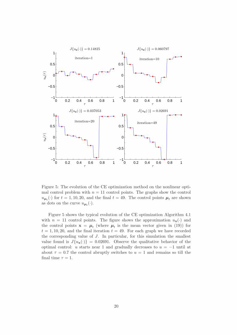
Figure 5: The evolution of the CE optimization method on the nonlinear opti-mal control problem with n = 11 control points. The graphs show the controluµt

(·) for t = 1, 10, 20, and the final t = 49. The control points µt are shownas dots on the curve uµt

(·).

Figure 5 shows the typical evolution of the CE optimization Algorithm 4.1with n = 11 control points. The figure shows the approximation ux(·) andthe control points x = µt (where µt is the mean vector given in (19)) fort = 1, 10, 20, and the final iteration t = 49. For each graph we have recordedthe corresponding value of J . In particular, for this simulation the smallestvalue found is J{ux(·)} = 0.02691. Observe the qualitative behavior of theoptimal control: u starts near 1 and gradually decreases to u = −1 until atabout τ = 0.7 the control abruptly switches to u = 1 and remains so till thefinal time τ = 1.

20

12

34

56

78

910

11

510

1520

2530

3540

45

0

0.1

0.2

0.3

0.4

0.5

0.6

0.7

0.8

0.9

control point iiteration t

{σt,i}

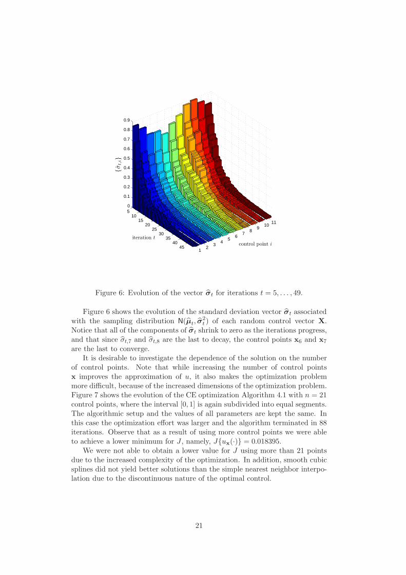
Figure 6: Evolution of the vector σt for iterations t = 5, . . . , 49.

Figure 6 shows the evolution of the standard deviation vector σt associatedwith the sampling distribution N(µt, σ

2t ) of each random control vector X.

Notice that all of the components of σt shrink to zero as the iterations progress,and that since σt,7 and σt,8 are the last to decay, the control points x6 and x7

are the last to converge.It is desirable to investigate the dependence of the solution on the number

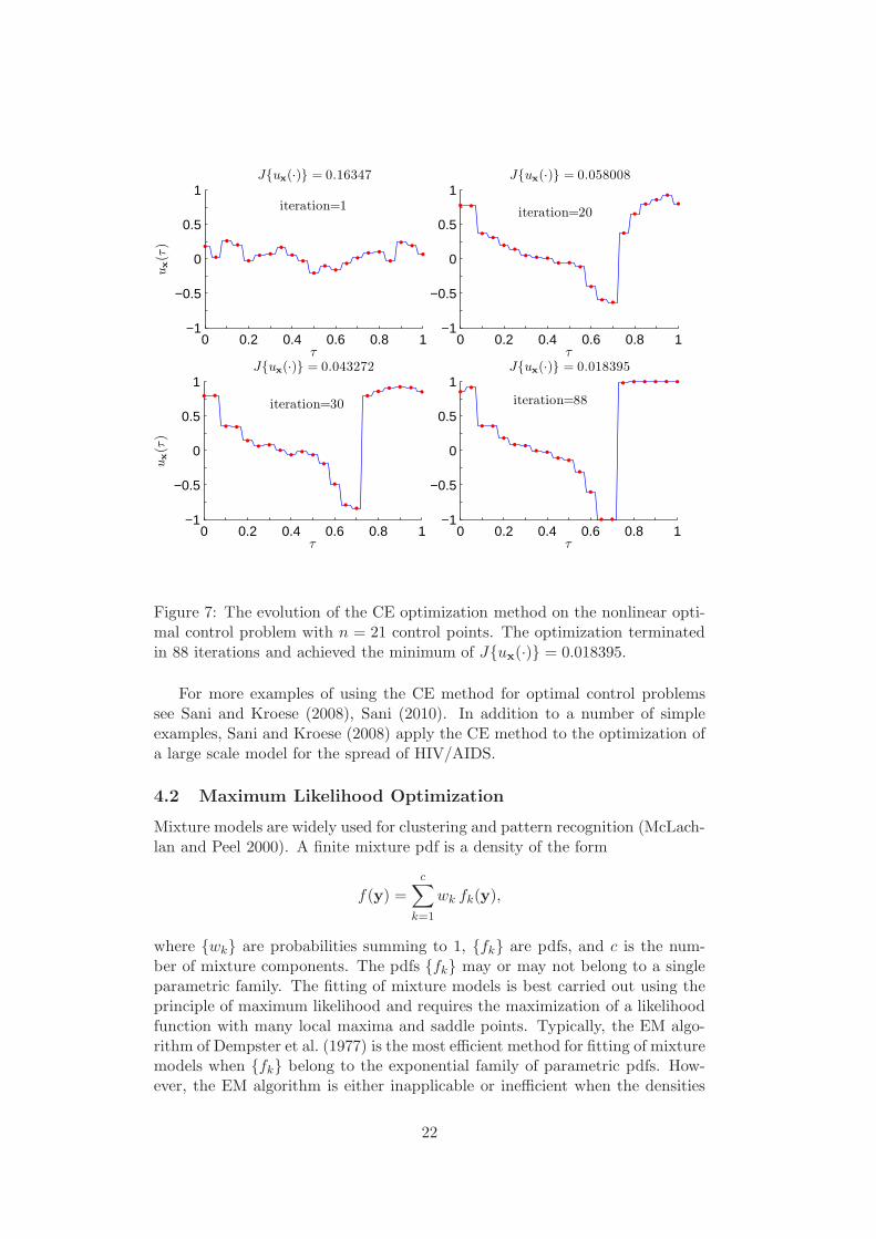
of control points. Note that while increasing the number of control pointsx improves the approximation of u, it also makes the optimization problemmore difficult, because of the increased dimensions of the optimization problem.Figure 7 shows the evolution of the CE optimization Algorithm 4.1 with n = 21control points, where the interval [0, 1] is again subdivided into equal segments.The algorithmic setup and the values of all parameters are kept the same. Inthis case the optimization effort was larger and the algorithm terminated in 88iterations. Observe that as a result of using more control points we were ableto achieve a lower minimum for J , namely, J{ux(·)} = 0.018395.

We were not able to obtain a lower value for J using more than 21 pointsdue to the increased complexity of the optimization. In addition, smooth cubicsplines did not yield better solutions than the simple nearest neighbor interpo-lation due to the discontinuous nature of the optimal control.

21

0 0.2 0.4 0.6 0.8 1−1

−0.5

0

0.5

1

τ

ux(τ

)J{ux(·)} = 0.16347

0 0.2 0.4 0.6 0.8 1−1

−0.5

0

0.5

1

τ

J{ux(·)} = 0.058008

0 0.2 0.4 0.6 0.8 1−1

−0.5

0

0.5

1

τ

ux(τ

)

J{ux(·)} = 0.043272

0 0.2 0.4 0.6 0.8 1−1

−0.5

0

0.5

1

τ

J{ux(·)} = 0.018395

iteration=88iteration=30

iteration=1iteration=20

Figure 7: The evolution of the CE optimization method on the nonlinear opti-mal control problem with n = 21 control points. The optimization terminatedin 88 iterations and achieved the minimum of J{ux(·)} = 0.018395.

For more examples of using the CE method for optimal control problemssee Sani and Kroese (2008), Sani (2010). In addition to a number of simpleexamples, Sani and Kroese (2008) apply the CE method to the optimization ofa large scale model for the spread of HIV/AIDS.

4.2 Maximum Likelihood Optimization

Mixture models are widely used for clustering and pattern recognition (McLach-lan and Peel 2000). A finite mixture pdf is a density of the form

f(y) =

c∑

k=1

wk fk(y),

where {wk} are probabilities summing to 1, {fk} are pdfs, and c is the num-ber of mixture components. The pdfs {fk} may or may not belong to a singleparametric family. The fitting of mixture models is best carried out using theprinciple of maximum likelihood and requires the maximization of a likelihoodfunction with many local maxima and saddle points. Typically, the EM algo-rithm of Dempster et al. (1977) is the most efficient method for fitting of mixturemodels when {fk} belong to the exponential family of parametric pdfs. How-ever, the EM algorithm is either inapplicable or inefficient when the densities

22

{fk} are not part of an exponential family or are not continuous with respectto some of its model parameters. For example, consider a mixture consistingof one d-dimensional Gaussian and c − 1 uniform densities on d-dimensionalrectangles:

f(y;θ) =w1 e−

12

Pdi=1(yi−ν1,i)

2/ς21,i

(2π)d2

∏di ς1,i

+c∑

k=2

wk

d∏

i=1

I{|yi − νk,i| < 1

2ςk,i

}

ςk,i. (24)

Here, (νk,1, . . . , νk,d) and (ςk,1, . . . , ςk,d) are the location and scale parametersof the k-th component, and

θ = ((ν1,1, . . . , νc,d), (ς1,1, . . . , ςc,d), (w1, . . . , wc))

summarizes all model parameters. The log-likelihood function given the datay1, . . . ,yn is S(θ) =

∑nj=1 ln f(yj ;θ), which is not continuous with respect

to all parameters, because the support of each uniform component dependson the scale parameters {ςk,i, k > 2}. We now show how to apply the CE

method to solve the optimization program θ = argmaxθ∈Θ S(θ), where Θ isthe set for which all ςk,i > ςlow > 0 for some threshold ςlow and {wk} areprobabilities summing to one. Note that ςlow must be strictly positive to ensurethat maxθ∈Θ S(θ) <∞.

In Step 2 of Algorithm 4.1 the population X1, . . . ,XN corresponds to ran-domly generated proposals for the parameter θ = X. Thus, the CE parametervectors µ and σ2 are of length (2d + 1)c, with the first d c elements associatedwith the location parameters of the mixture, the next d c elements associatedwith the scale parameters, and the last c elements associated with the mixtureweights. In particular, we sample the locations ν1,1, . . . , νc,d from the normaldistributions N(µ1, σ

21), . . . ,N(µc d, σ

2c d). To account for the constraints on the

scale parameters of the mixture we sample ς1,1, . . . , ςc,d from the normal dis-tributions N(µc d+1, σ

2c d+1), . . . ,N(µ2c d, σ

22c d) truncated to the set [ςlow,∞). To

generate the mixture weights {wk} we need to sample positive random vari-ables ω1, . . . , ωc such that

∑k ωk = 1. For this purpose we generate all weights

from truncated normal distributions in a random order (specified by a randompermutation), as in the following algorithm.

Algorithm 4.2 (Generation of Mixture Weights)

Require: The last c elements of the CE parameter vectors µ and σ2.Generate a random permutation π of 1, . . . , c.for k = 1, . . . , (c− 1) do

Generate wπ(k) from the normal distribution N(µ2dc+π(k), σ22dc+π(k)) trun-

cated to the interval [0, 1− (wπ(1) + · · · + wπ(k−1))].end forSet wπ(c) = 1− (wπ(1) + · · ·+ wπ(c−1)).return Random mixture weights w1, . . . , wc.

As a particular example, consider fitting the mixture model (24) to then = 200 random points depicted on Figure 8. The data are pseudo-randomvariables generated from (24) with c = 3, weights (w1, w2, w3) = (1/2, 1/4, 1/4),

23

location parameters

(ν1,1

ν1,2

)=

(00

),

(ν2,1

ν2,2

)=

(−2−2

),

(ν3,1

ν3,2

)=

(22

),

and scale parameters

(ς1,1

ς1,2

)=

(11

),

(ς2,1

ς2,2

)=

(ς3,1

ς3,2

)=

(44

).

−4 −3 −2 −1 0 1 2 3 4−4

−3

−2

−1

0

1

2

3

4

0

0.05

0.1

f(y

)

y1

y2

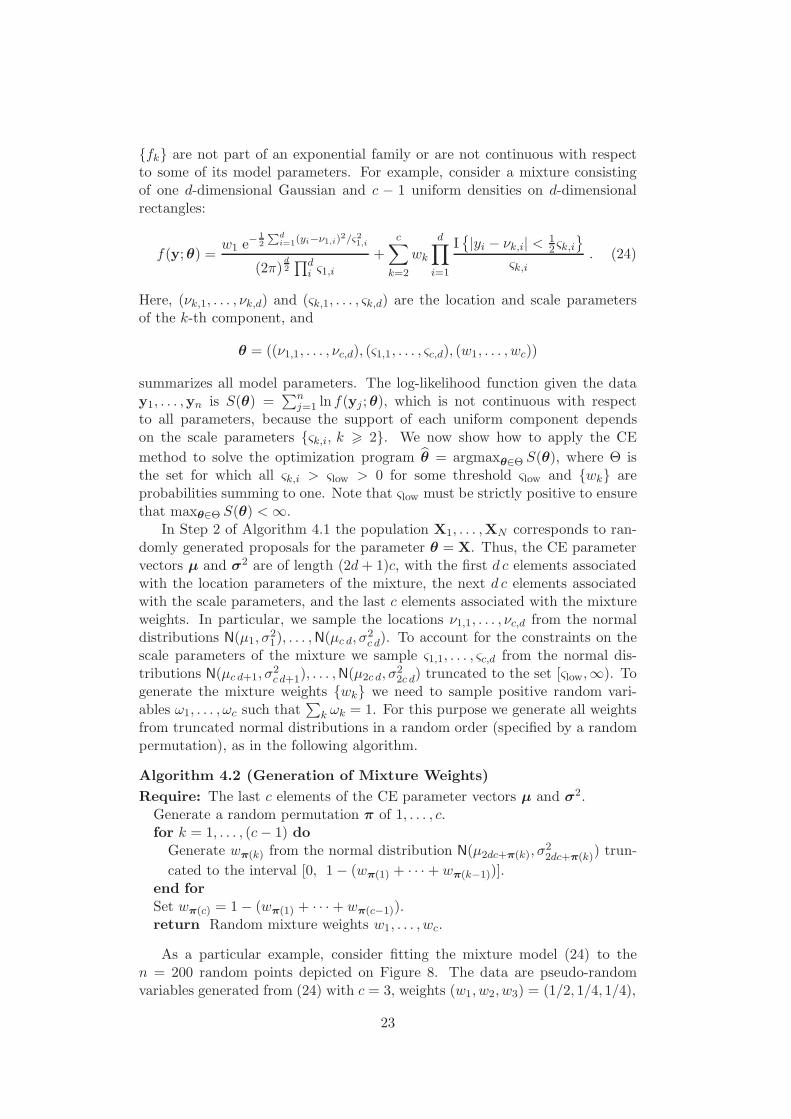
Figure 8: A sample of size 200 from a mixture of two uniform and a Gaussiandistributions. Superimposed is the contour plot of the fitted mixture densityf(y; θ).

We applied Algorithm 4.1 with N = 100, N e = 10, α = 0.5, ε = ςlow = 0.01,and µ0 = (1, . . . , 1) and σ0 = (10, . . . , 10). The algorithm terminated aftert = 89 iterations with the overall maximum log-likelihood of S(θ) = −707.7593.Figure 8 shows the estimated mixture model. The model appears to fit the datawell. In addition, the true value of the parameters θ gives S(θ) = −710.7937 <S(θ), which suggests that θ is the global maximizer. We found that for fittingmixture models the CE algorithm is not sensitive to the initial conditions andworks satisfactorily for 0.2 ≤ α ≤ 0.8.

24

5 Summary

We have described the CE method for combinatorial and continuous optimiza-tion. In summary, any CE algorithm for optimization involves the followingtwo main iterative phases:

1. Generate a random sample of objects in the search space X (trajecto-ries, vectors, etc.) according to a specified probability distribution.

2. Update or refit the parameters of that distribution based on the N e bestperforming samples (the so-called elite samples) using CE minimization.

An important part of the algorithm involves the selection of a suitable prob-ability density that allows for simple random variable generation and simpleupdating formulae (arising from the CE minimization) for the parameters ofthe density. For most optimization problems standard parametric models suchas the multivariate Bernoulli and Gaussian densities (for discrete and continu-ous problems, respectively) are adequate. Finally, the CE method is a robusttool for noisy continuous or discrete optimization problems.

References

G. Alon, D. P. Kroese, T. Raviv, and R. Y. Rubinstein. Application of thecross-entropy method to the buffer allocation problem in a simulation-basedenvironment. Annals of Operations Research, 134(1):137–151, 2005.

D. P. Bertsekas. Dynamic Programming and Optimal Control, volume I. AthenaScientific, third edition, 2007.

A. H. Borzabadi and M. Heidari. Comparison of some evolutionary algorithmsfor approximate solutions of optimal control problems. Australian Journal ofBasic and Applied Sciences, 4(8):3366–3382, 2010.

A. H. Borzabadi and H. H. Mehne. Ant colony optimization for optimal con-trol problems. Journal of Information and Computing Science, 4(4):259–264,2009.

Z. I. Botev and D. P. Kroese. Global likelihood optimization via the cross-entropy method with an application to mixture models. In Proceedings of the36th Winter Simulation Conference, pages 529–535, Washington, D.C., 2004.

A. Boubezoula, S. Paris, and M. Ouladsinea. Application of the cross en-tropy method to the GLVQ algorithm. Pattern Recognition, 41(10):3173–3178, 2008.

L. Busoniu, R. Babuska, B. De Schutter, and D. Ernst. Reinforcement Learningand Dynamic Programming using Function Approximators. Taylor & FrancisGroup, New York, 2010.

25

H. Cancela and M. E. Urquhart. Simulated annealing for communication net-work reliability improvements. In Proceedings of the XXI Latin AmericanConference On Informatics, pages 1413–1424, 1995.

K. Chepuri and T. Homem-de-Mello. Solving the vehicle routing problem withstochastic demands using the cross entropy method. Annals of OperationsResearch, 134(1):153–181, 2005.

I. Cohen, B. Golany, and A. Shtub. Resource allocation in stochastic, finite-capacity, multi-project systems through the cross entropy methodology. Jour-nal of Scheduling, 10(1):181–193, 2007.

A. Costa, J. Owen, and D. P. Kroese. Convergence properties of the cross-entropy method for discrete optimization. Operations Research Letters, 35(5):573–580, 2007.

P. T. de Boer, D. P. Kroese, S. Mannor, and R. Y. Rubinstein. A tutorial on thecross-entropy method. Annals of Operations Research, 134(1):19–67, 2005.

A. M. Leite de Silva, R. A. G. Fernandez, and C. Singh. Generating capac-ity reliability evaluation based on Monte Carlo simulation and cross-entropymethods. IEEE Transactions on Power Systems, 25(1):129–137, 2010.

A. P. Dempster, N. M. Laird, and D. B. Rubin. Maximum likelihood from in-complete data via the EM algorithm. Journal of the Royal Statistical Society,Series B, 39(1):1–38, 1977.

B. Dengiz, F. Altiparmak, and A. E. Smith. Local search genetic algorithmfor optimal design of reliable networks. IEEE Transactions on EvolutionaryComputation, 1(3):179–188, 1997.

J. R. Dormand and P. J. Prince. A family of embedded Runge-Kutta formulae.J. Comp. Appl. Math., 6:19–26, 1980.

T. Elperin, I. B. Gertsbakh, and M. Lomonosov. Estimation of network reli-ability using graph evolution models. IEEE Transactions on Reliability, 40(5):572–581, 1991.

D. Ernst, M. Glavic, G.-B. Stan, S. Mannor, L. Wehenkel, and Gif surYvette Supelec. The cross-entropy method for power system combinatorialoptimization problems. In Power Tech, 2007 IEEE Lausanne, pages 1290 –1295, Lausanne, 2007.

G. E. Evans, J. M. Keith, and D. P. Kroese. Parallel cross-entropy optimization.In Proceedings of the 2007 Winter Simulation Conference, pages 2196–2202,Washington, D.C., 2007.

J. Gu, P. W. Purdom, J. Franco, and B. W. Wah. Algorithms for the sat-isfiability (SAT) problem: A survey. In Satisfiability Problem: Theory andApplications, pages 19–152. American Mathematical Society, Providence, RI,1997.

26

P. Hintsanen, H. Toivonen, and P. Sevon. Fast discovery of reliable subnetworks.In 2010 International Conference on Advances in Social Network Analysisand Mining, pages 104 – 111, 2010.

H. H. Hoos and T. Stutzle. SATLIB: An online resource for research on SAT.In: SAT 2000, I. P. Gent, H. v. Maaren, T. Walsh, editors, pages 283–292.www.satlib.org, IOS Press, 2000.

J. Keith and D. P. Kroese. Sequence alignment by rare event simulation. InProceedings of the 2002 Winter Simulation Conference, pages 320–327, SanDiego, 2002.

H. Kellerer, U. Pferschy, and D. Pisinger. Knapsack Problems. Springer Verlag,first edition, 2004.

R. P. Kothari and D. P. Kroese. Optimal generation expansion planning via thecross-entropy method. In M. D. Rossetti, R. R. Hill, B. Johansson, A. Dunkin,and R. G. Ingalls, editors, Proceedings of the 2009 Winter Simulation Con-ference., pages 1482–1491, 2009.

D. P. Kroese, K.-P. Hui, and S. Nariai. Network reliability optimization viathe cross-entropy method. IEEE Transactions on Reliability, 56(2):275–287,2007a.

D. P. Kroese, S. Porotsky, and R. Y. Rubinstein. The cross-entropy methodfor continuous multi-extremal optimization. Methodology and Computing inApplied Probability, 8(3):383–407, 2006.

D. P. Kroese, R. Y. Rubinstein, and T. Taimre. Application of the cross-entropy method to clustering and vector quantization. Journal of GlobalOptimization, 37:137–157, 2007b.

Z. Liu, A. Doucet, and S. S. Singh. The cross-entropy method for blind mul-tiuser detection. In IEEE International Symposium on Information Theory,Chicago, 2004. Piscataway.

A. Lorincza, Z. Palotaia, and G. Szirtesb. Spike-based cross-entropy methodfor reconstruction. Neurocomputing, 71(16–18):3635–3639, 2008.

L. Margolin. On the convergence of the cross-entropy method. Annals of Op-erations Research, 134(1):201–214, 2005.

G. J. McLachlan and D. Peel. Finite Mixture Models. John Wiley & Sons, NewYork, 2000.

I. Menache, S. Mannor, and N. Basis function adaptation in temporal differencereinforcement learning. Annals of Operations Research, 134(1):215–238, 2005.

V. Pihur, S. Datta, and S. Datta. Weighted rank aggregation of cluster vali-dation measures: a Monte Carlo cross-entropy approach. Bioinformatics, 23(13):1607–1615, 2007.

27

D. Reichelt, F. Rothlauf, and P. Bmilkowsky. Designing reliable communica-tion networks with a genetic algorithm using a repair heuristic. In Evolution-ary Computation in Combinatorial Optimization, pages 177–186. Springer-Verlag, Heidelberg, 2007.

G. Rubino. Network reliability evaluation. In J. Walrand, K. Bagchi, and G. W.Zobrist, editors, Network Performance Modeling and Simulation, chapter 11.Blackwell Scientific Publications, Amsterdam, 1998.

G. Rubino and B. Tuffin. Rare Event Simulation. John Wiley & Sons, NewYork, 2009.

R. Y. Rubinstein. Optimization of computer simulation models with rare events.European Journal of Operational Research, 99(1):89–112, 1997.

R. Y. Rubinstein. The cross-entropy method for combinatorial and continuousoptimization. Methodology and Computing in Applied Probability, 1(2):127–190, 1999.

R. Y. Rubinstein. Combinatorial optimization, cross-entropy, ants and rareevents. In S. Uryasev and P. M. Pardalos, editors, Stochastic Optimization:Algorithms and Applications, pages 304–358, Dordrecht, 2001. Kluwer.

R. Y. Rubinstein and D. P. Kroese. The Cross-Entropy Method: A Unified Ap-proach to Combinatorial Optimization, Monte Carlo Simulation and MachineLearning. Springer-Verlag, New York, 2004.

R. Y. Rubinstein and D. P. Kroese. Simulation and the Monte Carlo Method.John Wiley & Sons, New York, second edition, 2007.

A. Sani. Stochastic Modelling and Intervention of the Spread of HIV/AIDS.PhD thesis, The University of Queensland, Brisbane, 2009.

A. Sani. The Spread of HIV/AIDS in Mobile Populations: Modelling, Analysis,Simulation. LAP LAMBERT Academic Publishing, Berlin, 2010.

A. Sani and D. P. Kroese. Controlling the number of HIV infectives in a mobilepopulation. Mathematical Biosciences, 213(2):103–112, 2008.

S. Senju and Y. Toyoda. An approach to linear programming with 0-1 variables.Management Science, 15(4):B196–B207, 1968.

Z. Szabo, B. Poczos, and A. Lorincz. Cross-entropy optimization for indepen-dent process analysis. In Independent Component Analysis and Blind SignalSeparation, volume 3889, pages 909–916. Springer-Verlag, Heidelberg, 2006.

A. Unveren and A. Acan. Multi-objective optimization with cross entropymethod: Stochastic learning with clustered pareto fronts. In IEEE Congresson Evolutionary Computation (CEC 2007), pages 3065–3071, 2007.

G.-B. Wang, H.-Z. Huang, Y. Liu, X. Zhang, and Z. Wang. Uncertainty estima-tion of reliability redundancy in complex systems based on the Cross-Entropymethod. Journal of Mechanical Science and Technology, 23:2612–2623, 2009.

28

J.-M. Won and F. Karray. Cumulative update of all-terminal reliability forfaster feasibility decision. IEEE Transactions on Reliability, 59(3):551–562,2010.

Y. Wu and C. Fyfe. Topology perserving mappings using cross entropy adapta-tion. In 7th WSEAS international conference on artificial intelligence, knowl-edge engineering and data bases, Cambridge, 2008.

A. Wuerl, T. Crain, and E. Braden. Genetic algorithm and calculus ofvariations-based trajectory optimization technique. Journal of spacecraft androckets, 40(6):882–888, 2003.

29