Working Paper

THE CONTRIBUTION OFSECTORAL PRODUCTIVITYTO INFLATION IN GREECE

No. 63 November 2007

Heather D. GibsonJim Malley

BANK OF GREECE Economic Research Department – Special Studies Division 21, Ε. Venizelos Avenue GR-102 50 Αthens Τel: +30210-320 3610 Fax: +30210-320 2432 www.bankofgreece.gr Printed in Athens, Greece at the Bank of Greece Printing Works. All rights reserved. Reproduction for educational and non-commercial purposes is permitted provided that the source is acknowledged. ISSN 1109-6691

THE CONTRIBUTION OF SECTORAL PRODUCTIVITY DIFFERENTIALS TO INFLATION IN GREECE

Heather D Gibson Bank of Greece

Jim Malley

University of Glasgow and CESifo

ABSTRACT This paper estimates the magnitude of the Balassa-Samuelson effect for Greece. We calculate the effect directly, using sectoral national accounts data, which permits estimation of total factor productivity (TFP) growth in the tradeables and nontradeables sectors. Our results suggest that it is difficult to produce one estimate of the BS effect. Any particular estimate is contingent on the definition of the tradeables sector and the assumptions made about labour shares. Moreover, there is also evidence that the effect has been declining through time as Greek standards of living have caught up on those in the rest of the world and as the non-tradeables sector within Greece catches up with the tradeables. Keywords: Balassa-Samuelson effect, inflation, productivity JEL codes: E31; F36; F41 Acknowledgments: We would like to thank a number of people at the Bank of Greece who have helped in preparing this paper. Presentations to the Monetary Policy Council yielded useful insights and comments and we would particularly like to thank George Demopoulos. Additionally, thanks are due to George Tavlas who commented on the paper at length as well as several colleagues who took time to discuss data issues with us, including Nick Zonzilos, Isaak Sampethai, and, especially, Daphne Nikolitsas. We would also like to thank Ioannis Papadogeorgis for his help in obtaining data from the OECD. The opinions and analysis presented in the paper are those of the authors and do not necessarily coincide with those of either the Bank of Greece or the Eurosystem.

Correspondence: Heather Gibson, Economic Research Department, Bank of Greece, 21, E. Venizelos Ave., 102 50 Athens, Greece Tel. +30210-320 2415 Fax +30210-320 2432 email: hgibson@bankofgreece.gr

5

1. Introduction

The existence of significant inflation differentials in the euro area and their

potential impact on the competitiveness of those countries with higher inflation have

led to increased interest in the magnitude of the Balassa-Samuelson (hereafter BS)

effect. To the extent that an inflation differential between a particular country and its

main trading partners is entirely a consequence of this effect, it will not impact on that

country’s competitiveness vis-à-vis its trading partners. In a monetary union, where

the option of using the nominal exchange rate to alter competitiveness among the

members has been given up, this is a reassuring result because it implies that inflation

differentials do not need to be offset through nominal exchange rate adjustments1.

The BS effect (originating from the work of Balassa, 1964, and Samuelson,

1964, on reasons for departures from purchasing power parity) starts from the basic

observation that productivity in the tradeables (and, by implication, the more

dynamic) sector usually rises faster than in the non-tradeables sector. This situation is

especially true in countries with lower per capita income levels that are catching up

countries that have higher per capita income levels2. Any increase in tradeables

productivity raises nominal and real wages, leaving tradeable goods prices unchanged.

On the assumption that nominal wages in both sectors are equalised because of

perfect labour mobility between the two sectors, this result implies that prices in the

non-tradeables sector have to rise to compensate producers for the increase in costs.

The consequence is a rise in the non-tradeables/tradeable price ratio. However, the

higher implied aggregate price level does not imply a loss of competitiveness.

This paper estimates the magnitude of the BS effect for Greece to determine

the extent to which its inflation differential with the euro area can be attributed to it.

The Greek case is an interesting one. Since 2001, when Greece entered the euro area,

1 The BS effect may exist irrespective of the exchange rate regime. For countries with flexible exchange rates, which are catching up, the BS effect will again imply real appreciation without the appreciation involving a loss in competitiveness. For countries that are planning on joining a monetary union or some form of exchange rate system (such as ERM II), some measure of the extent of the BS effect may be helpful in setting the exchange rate at which entry will take place. Many papers deal with the extent of the BS effect in new EU Member States (De Broeck and Slok, 2001; Arratibel, Rodriguez-Pollenzuela and Thimann, 2002; Flek, Markova and Podpiera, 2002; Fischer, 2002; Mihaljek and Klau, 2003; Crespo-Cuaresma, Fidrmuc and MacDonald, 2005; Egert, 2006). See Doyle, Kuijs and Jiang (2001) for a review of earlier studies. 2 See, for example, the extensive discussion in Ito, Isard and Symansky (1997) on the particular relevance of the BS effect for fast growth economies. They argue that it is in such countries that the differentials in productivity increases are greater.

6

Greek inflation has been consistently above that of the euro area average (something

which is also true in several other countries such as Spain and Portugal). Greece also

has, or at least had, significantly lower per capita income than the euro area average

(Figure 1) and has experienced two periods of rapid catch-up separated by relative

stagnation. It is thus a prime candidate for experiencing the BS effect.

Much of the existing empirical work on the BS effect either tests for its

existence, but does not estimate its magnitude, or, uses rather ad hoc empirical

specifications which have little grounding in theory. In contrast to most previous

studies, we assess the effect by calculating it directly. To this end, we use data for the

tradeable and nontradeables sectors, which permits estimation of total factor

productivity (TFP) growth in both sectors. By doing so, we are able to determine the

size of the BS effect and, hence, the proportion of inflation attributable to it. That we

consider TFP growth in calculating the size of the BS effect has the advantage that it

is consistent with theory3. One possible criticism of our approach is that we focus

exclusively on what is known as the domestic version of the BS effect (Baumol and

Bowen, 1966) – that is, we do not take account of the fact that the countries with

which Greece trades may also be experiencing a BS effect. However, when one

considers that Greece’s main trading partners in the euro area are typically at a much

higher level of development and have been experiencing lower growth rates than

Greece, the magnitude of the BS effect in such countries is likely to be relatively

insignificant4.

The results suggest that it is misleading to single out a constant BS effect

throughout the entire estimation period. On the contrary, the evidence is consistent

with a strong BS effect of around 3 percentage points during the 1960s and early

1970s (the first period of catch-up), a shrinking BS effect, which for some estimates

even turned negative, during the late 1970s and 1980s, before rising again to around

3 The vast majority of the literature, whilst recognising that it is total factor productivity differences between the two sectors that determine the size of the BS effect, uses relative labour productivity in empirical analyses. An exception is Katsimi (2004). 4 Evidence supporting the fact that the BS effect is insignificant in more highly developed countries comes from the strong association between real exchange rate appreciation and economic development (Ito, Isard and Symansky, 1997; Drine and Rault, 2003; 2005). In the literature that actually considers the BS effect in developed countries, the evidence about its existence is mixed. One problem preventing a more definitive conclusion is that often panel data techniques are used (and hence the evidence in favour of a BS effect is a general average for all countries in the sample) and/or the actual size of the effect is not calculated. See Faria and Leon-Ledesma (2000), Ortega (2003), Katsimi (2004) and Drine and Rault (2005).

7

1.5-2.0 percentage points in the second half of the 1990s (the second major period of

catch-up). Not surprisingly, recent data suggest that as Greek standards of living on

average approach those of the euro area (or EU) as a whole and as the size of the

nontraded sector diminishes in the light of the break down of traditional barriers to

trade in certain goods and services due to globalisation and technological

development, the size of the BS effect has declined significantly, to around 0.5 of a

percentage point, if not lower. Considering that many other EU countries also have a

BS effect, this finding implies that the relative effect for Greece (the so-called

international BS effect) in all probability disappears. As we show, this result is

reasonably robust across different definitions of the tradeable and non-tradeables

sectors.

The remainder of the paper is organised as follows. In Section 2, we describe

the theoretical framework and derive the key relations from which the BS effect is

calculated. In section 3, we provide some stylised facts about the Greek economy

including sectoral labour productivity growth differentials, total factor productivity

growth differentials and inflation differentials. In section 4, we outline our empirical

methodology and present the results. Section 5 provides conclusions.

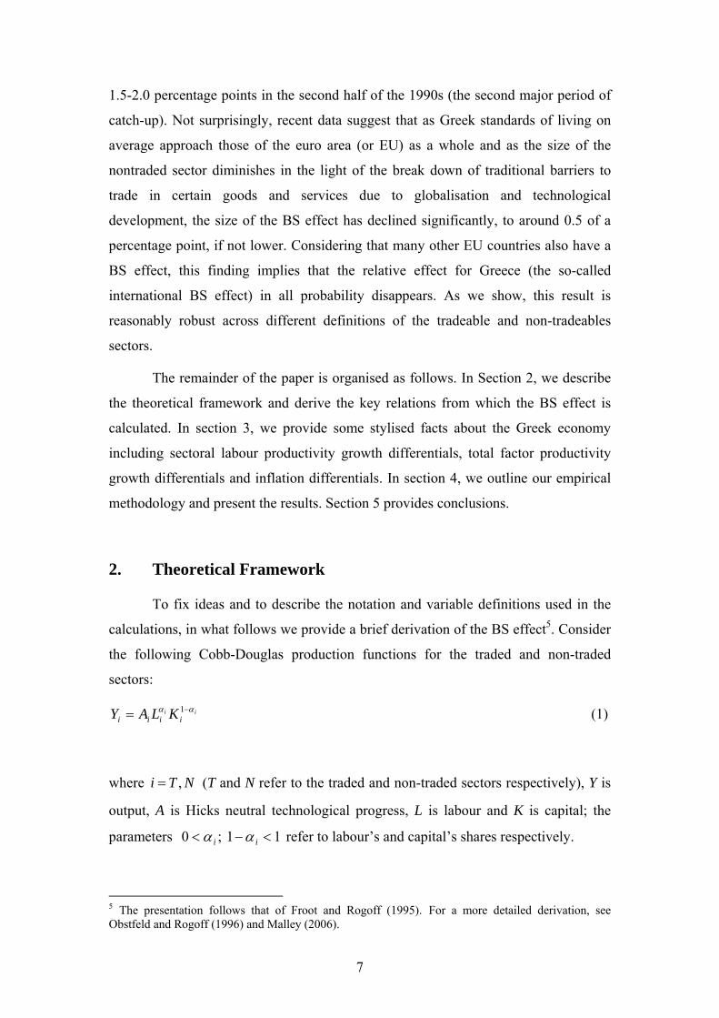
2. Theoretical Framework

To fix ideas and to describe the notation and variable definitions used in the

calculations, in what follows we provide a brief derivation of the BS effect5. Consider

the following Cobb-Douglas production functions for the traded and non-traded

sectors:

iiiiii KLAY αα −= 1 (1)

where ,i T N= (T and N refer to the traded and non-traded sectors respectively), Y is

output, A is Hicks neutral technological progress, L is labour and K is capital; the

parameters 11 ;0 <−< ii αα refer to labour’s and capital’s shares respectively.

5 The presentation follows that of Froot and Rogoff (1995). For a more detailed derivation, see Obstfeld and Rogoff (1996) and Malley (2006).

8

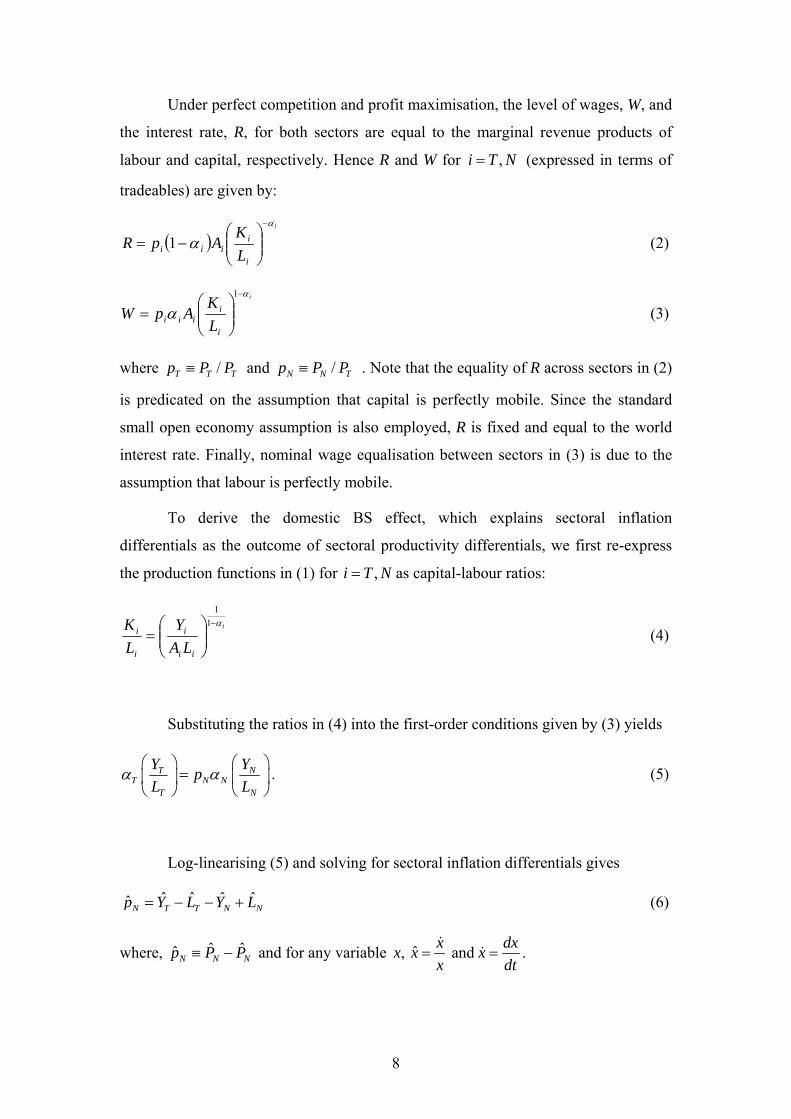
Under perfect competition and profit maximisation, the level of wages, W, and

the interest rate, R, for both sectors are equal to the marginal revenue products of

labour and capital, respectively. Hence R and W for ,i T N= (expressed in terms of

tradeables) are given by:

( )i

i

iiii L

KApR

α

α−

⎟⎟⎠

⎞⎜⎜⎝

⎛−= 1 (2)

i

i

iiii L

KApW

α

α−

⎟⎟⎠

⎞⎜⎜⎝

⎛=

1

(3)

where / T T Tp P P≡ and / N N Tp P P≡ . Note that the equality of R across sectors in (2)

is predicated on the assumption that capital is perfectly mobile. Since the standard

small open economy assumption is also employed, R is fixed and equal to the world

interest rate. Finally, nominal wage equalisation between sectors in (3) is due to the

assumption that labour is perfectly mobile.

To derive the domestic BS effect, which explains sectoral inflation

differentials as the outcome of sectoral productivity differentials, we first re-express

the production functions in (1) for ,i T N= as capital-labour ratios:

i

ii

i

i

i

LAY

LK α−

⎟⎟⎠

⎞⎜⎜⎝

⎛=

11

(4)

Substituting the ratios in (4) into the first-order conditions given by (3) yields

NTT N N

T N

YY pL L

α α⎛ ⎞⎛ ⎞

= ⎜ ⎟⎜ ⎟⎝ ⎠ ⎝ ⎠

. (5)

Log-linearising (5) and solving for sectoral inflation differentials gives

ˆ ˆ ˆ ˆˆ N T T N Np Y L Y L= − − + (6)

where, ˆ ˆˆ N N Np P P≡ − and for any variable ˆ, and x dxx x xx dt

= =&

& .

9

Log-linearising the production functions in (1) and substituting the resulting

expressions into (6) yields:

( ) ( ) ( ) ( )ˆ ˆ ˆ ˆ ˆ ˆ ˆ ˆ ˆ ˆˆ N T N T T T T T N N N N Np A A K L K L K L K Lα α= − − − + − + − − − (7)

where the Solow residual for ,i T N= is defined as ( )ˆ ˆ ˆ ˆ1i i i i i iA Y L Kα α≡ − − − .

Since R is fixed, via the small open economy assumption, the first-order

conditions in (2) imply ( )ˆˆ ˆ T

T TT

AK Lα

− = and ( )ˆˆˆ ˆ N N

N NN

p AK Lα+

− = . Substituting these

into (7) gives a relation stating that the difference between non-traded and traded

inflation, ˆ Np , is driven by the difference between TFP growth in the traded, ˆTA , and

the non-traded sectors, ˆNA , i.e.,

ˆ ˆˆ NN T N

T

p A Aαα

= − . (8)

Also, note that even if TFP growth is equal in the traded and non-traded sectors,

positive inflation differentials will nevertheless occur when N Tα α> . Given that

aggregate inflation, P̂ , can be expressed as a weighted average of traded and non-

traded inflation6, we can rewrite (8) as

( )ˆ ˆ ˆ1T NP P pγ= + − . (9)

Thus, aggregate inflation can be decomposed into the sum of inflation in the

traded sector, T̂P and the weighted sectoral inflation differential, or the domestic BS

effect7, ( ) ˆ1 Npγ− .

The mechanism underlying the BS effect is subject to several criticisms. For

example, it assumes perfect labour mobility between the traded and nontraded goods

6 That is, ( )ˆ ˆ ˆ1T NP P Pγ γ= + − , where /TY Yγ = and ( )1- /NY Yγ = . 7 In contrast, the international BS effect is: ( )[ ]* *ˆ ˆ ˆ ˆ1 N NP P p pγ− = − − , where the “stars” refer to corresponding foreign values of aggregate inflation and sectoral inflation differentials respectively. In the literature, the domestic version is also referred to as the Baumol-Bowen (1966) effect.

10

sectors (which is the mechanism underlying wage equalisation across the two sectors)

as well as a more dynamic, faster-growing tradeables sector. Nevertheless, to the

extent that there is a systematic difference between inflation rates in the tradeables

and nontradeables sectors, changes in the competitive position of a country will not be

inferable from the difference between domestic and foreign inflation rates (along with

exchange rate changes, where appropriate). Differential productivity growth rates

between tradeables and nontradeables sectors, combined with perfect labour mobility

between the two sectors, may be one reason that tradeables inflation is systematically

different from that of nontradeables8.

3. Data, Methodology and Results

The approach to empirical estimation of the BS effect in this paper is to

calculate it directly using production functions for both the traded and nontraded

goods sectors. This allows us to generate a sectoral TFP series for Greece, which, in

turn, can be used to estimate the BS effect using equations (8) and (9) above. As noted

above, this approach differs from the predominant methodologies used in the

literature (Sinn and Reutter, 2002, are an exception although they use only labour

productivity differentials). In a first approach, ad hoc relations are estimated to

explain either relative prices (or inflation rates) between the two sectors as a function

of, among other variables, some measure of relative productivities (Flek, Markova

and Podpiera, 2002; Mihaljek and Klau, 2003; Katsimi, 2004; Egert, 2006) 9. A

second approach estimates the real exchange rate as a function of relative

productivities between the two sectors (Faria and Leon-Ledesma, 2000; De Broek and

Slok, 2001; Fischer, 2002) or simply the level of economic development (Drine and

Rault, 2003; 2005)10. A third approach focuses on inflation differentials in the euro

8 Other mechanisms, however, could also generate such a result including systematic differential productivity growth combined with centralised wage bargaining, which tends to lead to similar increases in wages across sectors irrespective of sectoral productivity developments. 9 A variation on this theme is provided by Arratibel, Rodriguez-Pollenzuella and Thirman (2002), who estimate separate equations for domestic inflation, tradeables inflation and non-tradeables inflation augmented by productivity in manufacturing. 10 A variation on the real exchange rate equations is the paper by Crespo-Cuaresma, Fidramic and MacDonald (2005), which estimates a monetary model of the nominal exchange rate extended to include the price of non-tradeables relative to tradeables. A non-econometric approach is used by Ortega (2003) and ECB (2003), under which inflation differentials are decomposed into the purchasing power parity condition in the traded goods sector along with mark-ups, nominal wages and labour productivity differentials between the nontraded and traded goods sectors.

11

area (Alberola-Ila and Tyrvainen, 1998; Sinn and Reutter, 2001; Canzoneri et al,

2002; Lommatzsch and Tober, 2006). To the extent that euro area countries

experience different BS effects, so inflation differentials between them can be

justified. These papers calculate an implied inflation rate for euro area member

countries based on productivity differentials and the share of non-tradeables in

production (as given in equation (9) above, with productivity differentials referring to

labour productivity growth and not TFP growth as we use here). Data periods focus

on the 1970s, 1980s and into the 1990s. The results suggest inflation differentials of 2

percentage points (Alberola-Ila and Tyrvainen, 1998), 2.5 percentage points

(Canzoneri et al, 2002; Lommatzsch and Tober, 2006) and, even, 4 percentage points

(Sinn and Reutter, 2001).

Empirical work on the Greek economy is hard to come by, mainly, we suspect,

because sectoral national accounts data are not readily available on a consistent basis

over a long time period. Bragoudakis and Moschos (2000) use cointegration

techniques to examine the relationship between relative prices, relative labour

productivities and relative wages over the period 1962-97. They find no evidence of

cointegration, which implies that a BS effect alone cannot explain relative price

movements. Their methodology does not permit estimation of the size of any BS

effect.

Sinn and Reutter (2001) calculate a minimum inflation rate for Greece of over

4% based on labour productivity differentials between traded and nontraded goods

sectors for the period 1991-96 and the assumption that all countries should have zero

or positive inflation rates. This suggests a BS effect which is large and is in sharp

contrast to Lommatzsch and Tober (2006) who find that Greek inflation should be

below the 2% rate assumed for the euro area as a whole. This latter result is again

based on labour productivity growth differentials, but covers the later period 1995-

2004.

The most comprehensive study of the BS effect in Greece is that of Swagel

(1999). He estimates that the BS effect contributed on average 1 percentage point per

annum to inflation over the period 1960-1996. This is calculated by estimating the

long-run cointegrating relationship between relative prices and relative total factor

productivities (relative wages were found not to have an impact in the Greek case)

and then adjusting the sectoral inflation differential (as given in equation (8)) for the

12

share of non-tradeables in production. Over the later period, 1990-96, the estimated

BS effect is even larger (around 1.7 percentage points)11.

3.1 Data

Our approach to estimating the BS effect, ( ) ˆ1 Npγ− , directly requires data for

output in traded and nontraded sectors (here measured by gross value added), along

with sectoral data on gross fixed capital formation (to enable sectoral capital stocks to

be compiled) and employment. Sectoral price data are calculated from the CPI sub-

categories. None of these data are available in “ready-made” form for the period

1960-2003; consequently we had to construct these data. Details about how the

database was constructed are provided in the data appendix12.

A critical, but difficult, assumption in the calculation of the BS effect concerns

the definition of the tradeables and nontradeables sectors. The difficulty arises for

several reasons. First, there is some controversy over what goods or services are best

characterised as tradeable. Consider the following examples. (1) Some of the

literature includes agriculture in non-tradeables because the existence of extensive

subsidies and administered prices implies that the sector does not function according

to market principles; some others exclude it altogether from their study. Bragoudakis

and Moschos (2000), in their analysis of Greek data, argue that the large proportion of

self-employment in the agriculture sector in Greece renders the link between wages

and productivity tenuous13. (2) In the Greek context, an important tradeable is

tourism. This circumstance might generate a case for including hotels and restaurants,

along with transport, in the tradeables sector, even though parts of these sectors are

clearly nontradeable.

11 The size of the BS effect for the more recent period is calculated using the parameters estimated over the whole period along with productivity differentials and inflation differentials for the period 1990-96. Swagel (1999) defines the tradeables sector as including mining and quarrying and manufacturing. Agriculture is excluded from the sample altogether. 12 Unfortunately, a lack of data on gross fixed capital formation by sector between 2004 and 2005 makes updating impossible. 13 Administered prices are not just a feature of agriculture. Other goods and services are also subject to regulation and there is evidence that prices in these sectors behave differentially from other services (Lunnemann and Matha, 2005; Egert et al., 2006). In the euro area, administered prices (for both goods and services and whether they are “fully” or “mainly” administered) account for around 13.8% of the Harmonised Index of Consumer Prices (HICP). Fully administered prices have a weight of 3.4% in the HICP. In Greece, the figures are similar at 12.3% and 4.5%, respectively. This compares with around 15-25% in most transition economies (Egert et al., 2006, Table A1).

13

Second, the situation might arise in which, with time, a good that was

previously considered to be a nontradeable has become tradeable, perhaps due to

changes in technology or government policy. For example, in the past, transport and

communications were considered nontradeable services. Today, with the deregulation

of these markets and their opening up to global competition, they could be considered

tradeables. A similar argument applies to financial intermediation and business

services.

Third, even if we could agree on what constitutes tradeable goods and

services, the sectoral accounts may not permit us to define tradeables and

nontradeables sectors exactly as we would like. In particular, frequent changes in

national account methodology make it very difficult to calculate a medium-term

concept like the BS effect.

Our approach here is to consider a variety of definitions of

tradeables/nontradeables, as defined in Table 1. That table provides five frequently

used definitions of tradeables and nontradeables and the availability of Greek data

corresponding to each definition. For the first three definitions, we can calculate the

BS effect for the whole time period under consideration in this study. This has the

advantage that we can calculate average BS effects over long periods in order to

identify any trends, which minimises the impact of cyclical considerations on TFP

growth estimates. For the latter two (broad) definitions of the tradeables sector, we

can provide estimates of the effect only from 1995.

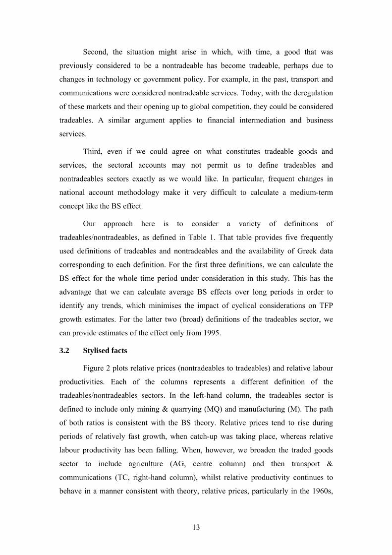
3.2 Stylised facts

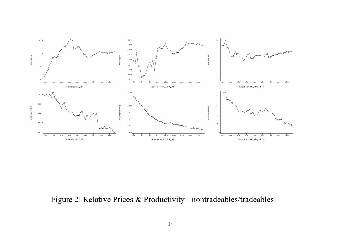
Figure 2 plots relative prices (nontradeables to tradeables) and relative labour

productivities. Each of the columns represents a different definition of the

tradeables/nontradeables sectors. In the left-hand column, the tradeables sector is

defined to include only mining & quarrying (MQ) and manufacturing (M). The path

of both ratios is consistent with the BS theory. Relative prices tend to rise during

periods of relatively fast growth, when catch-up was taking place, whereas relative

labour productivity has been falling. When, however, we broaden the traded goods

sector to include agriculture (AG, centre column) and then transport &

communications (TC, right-hand column), whilst relative productivity continues to

behave in a manner consistent with theory, relative prices, particularly in the 1960s,

14

do not, especially with regard to the third definition of traded goods. That is, the

relative price of nontradeables to tradeables falls, either for a short period between

1960 and 1965 (when agriculture is included as a tradeable) or for the period up until

the mid-1970s (when both agriculture and transport & communications are included

in tradeables). This result is a consequence of the fact that the prices of these

products/services were rising quite rapidly during the 1960s – moving them from

nontradeables serves to dampen nontradeable prices and adding them to tradeables

helps inflate tradeable prices. The net result is a fall in the price of nontradeables

relative to tradeables.

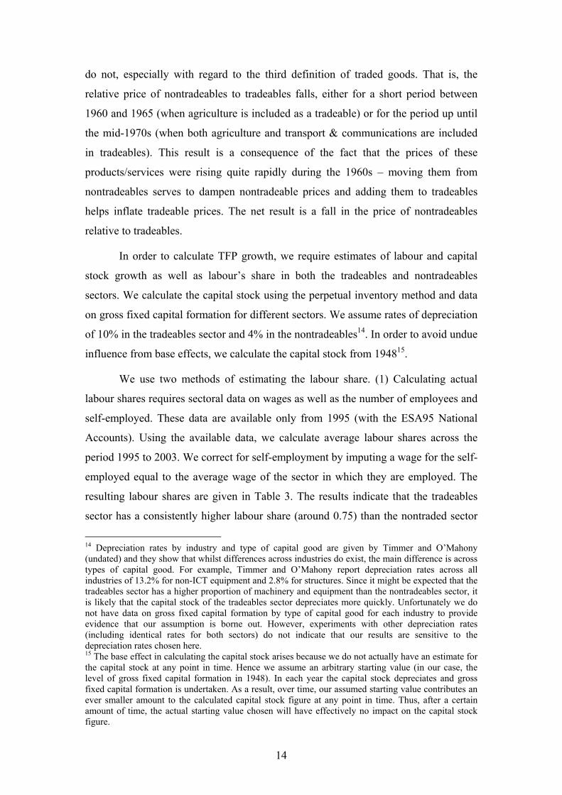
In order to calculate TFP growth, we require estimates of labour and capital

stock growth as well as labour’s share in both the tradeables and nontradeables

sectors. We calculate the capital stock using the perpetual inventory method and data

on gross fixed capital formation for different sectors. We assume rates of depreciation

of 10% in the tradeables sector and 4% in the nontradeables14. In order to avoid undue

influence from base effects, we calculate the capital stock from 194815.

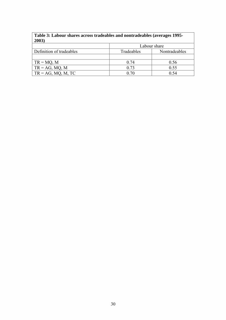
We use two methods of estimating the labour share. (1) Calculating actual

labour shares requires sectoral data on wages as well as the number of employees and

self-employed. These data are available only from 1995 (with the ESA95 National

Accounts). Using the available data, we calculate average labour shares across the

period 1995 to 2003. We correct for self-employment by imputing a wage for the self-

employed equal to the average wage of the sector in which they are employed. The

resulting labour shares are given in Table 3. The results indicate that the tradeables

sector has a consistently higher labour share (around 0.75) than the nontraded sector

14 Depreciation rates by industry and type of capital good are given by Timmer and O’Mahony (undated) and they show that whilst differences across industries do exist, the main difference is across types of capital good. For example, Timmer and O’Mahony report depreciation rates across all industries of 13.2% for non-ICT equipment and 2.8% for structures. Since it might be expected that the tradeables sector has a higher proportion of machinery and equipment than the nontradeables sector, it is likely that the capital stock of the tradeables sector depreciates more quickly. Unfortunately we do not have data on gross fixed capital formation by type of capital good for each industry to provide evidence that our assumption is borne out. However, experiments with other depreciation rates (including identical rates for both sectors) do not indicate that our results are sensitive to the depreciation rates chosen here. 15 The base effect in calculating the capital stock arises because we do not actually have an estimate for the capital stock at any point in time. Hence we assume an arbitrary starting value (in our case, the level of gross fixed capital formation in 1948). In each year the capital stock depreciates and gross fixed capital formation is undertaken. As a result, over time, our assumed starting value contributes an ever smaller amount to the calculated capital stock figure at any point in time. Thus, after a certain amount of time, the actual starting value chosen will have effectively no impact on the capital stock figure.

15

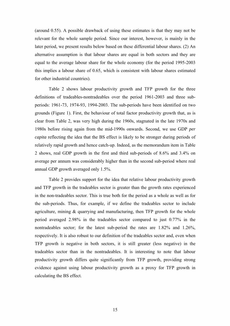
(around 0.55). A possible drawback of using these estimates is that they may not be

relevant for the whole sample period. Since our interest, however, is mainly in the

later period, we present results below based on these differential labour shares. (2) An

alternative assumption is that labour shares are equal in both sectors and they are

equal to the average labour share for the whole economy (for the period 1995-2003

this implies a labour share of 0.65, which is consistent with labour shares estimated

for other industrial countries).

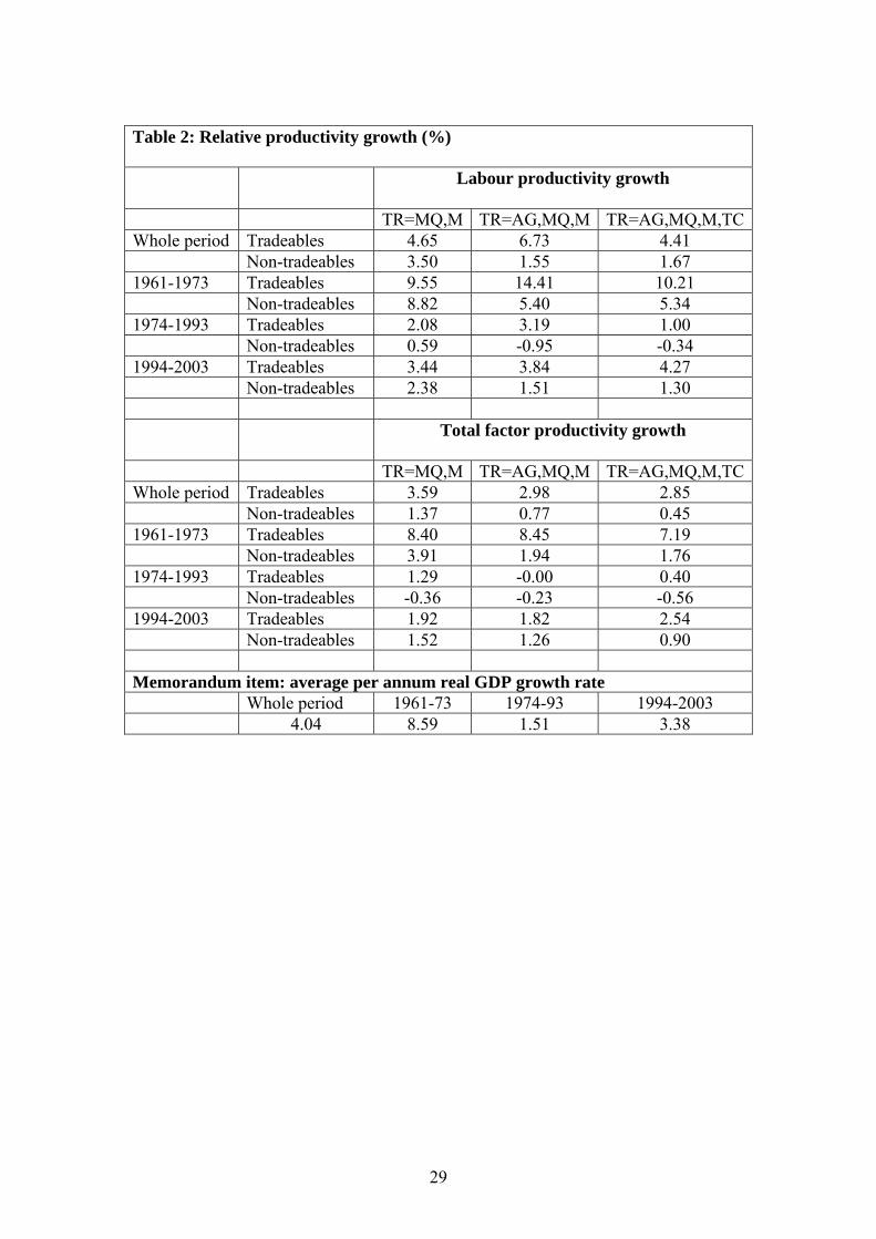
Table 2 shows labour productivity growth and TFP growth for the three

definitions of tradeables-nontradeables over the period 1961-2003 and three sub-

periods: 1961-73, 1974-93, 1994-2003. The sub-periods have been identified on two

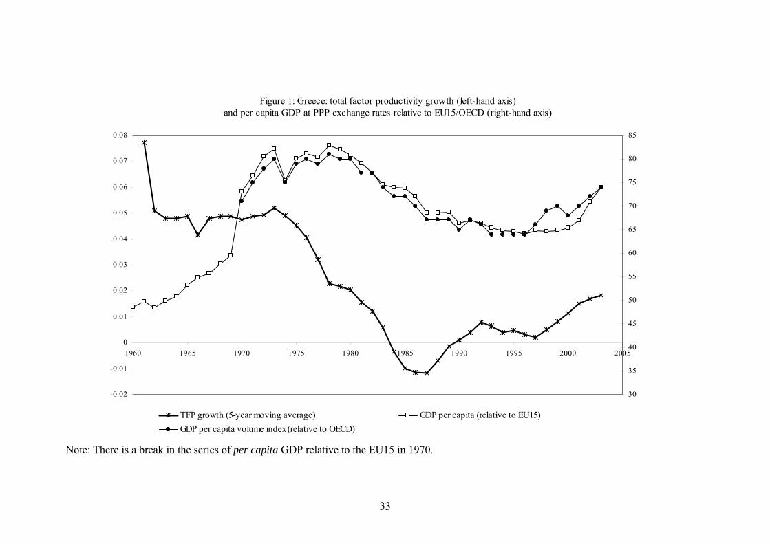
grounds (Figure 1). First, the behaviour of total factor productivity growth that, as is

clear from Table 2, was very high during the 1960s, stagnated in the late 1970s and

1980s before rising again from the mid-1990s onwards. Second, we use GDP per

capita reflecting the idea that the BS effect is likely to be stronger during periods of

relatively rapid growth and hence catch-up. Indeed, as the memorandum item in Table

2 shows, real GDP growth in the first and third sub-periods of 8.6% and 3.4% on

average per annum was considerably higher than in the second sub-period where real

annual GDP growth averaged only 1.5%.

Table 2 provides support for the idea that relative labour productivity growth

and TFP growth in the tradeables sector is greater than the growth rates experienced

in the non-tradeables sector. This is true both for the period as a whole as well as for

the sub-periods. Thus, for example, if we define the tradeables sector to include

agriculture, mining & quarrying and manufacturing, then TFP growth for the whole

period averaged 2.98% in the tradeables sector compared to just 0.77% in the

nontradeables sector; for the latest sub-period the rates are 1.82% and 1.26%,

respectively. It is also robust to our definition of the tradeables sector and, even when

TFP growth is negative in both sectors, it is still greater (less negative) in the

tradeables sector than in the nontradeables. It is interesting to note that labour

productivity growth differs quite significantly from TFP growth, providing strong

evidence against using labour productivity growth as a proxy for TFP growth in

calculating the BS effect.

16

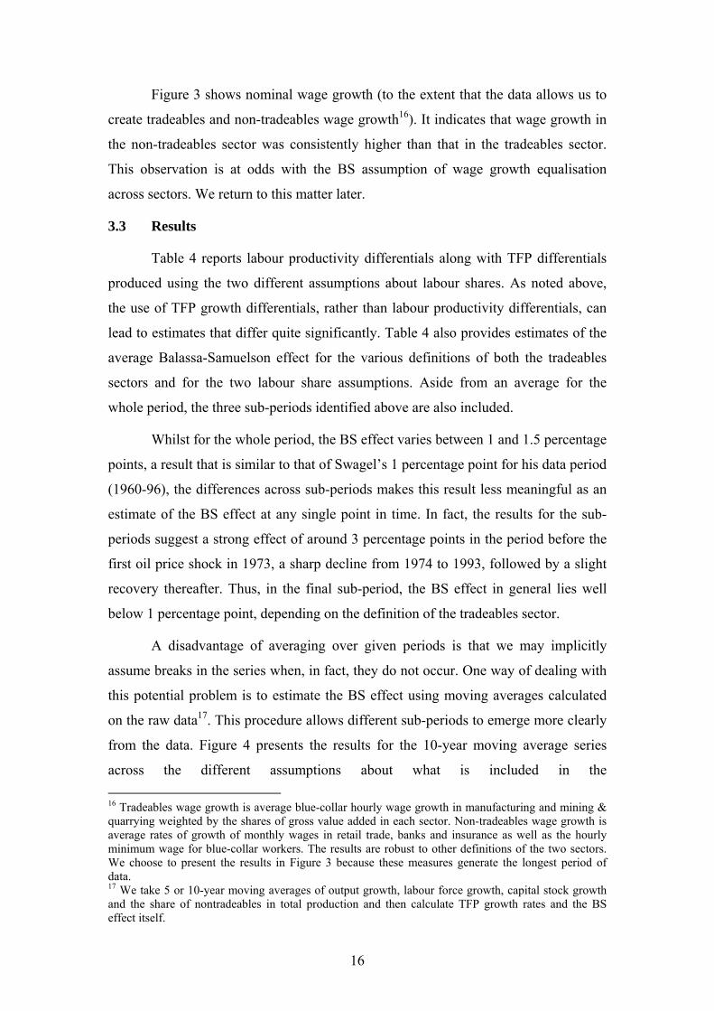
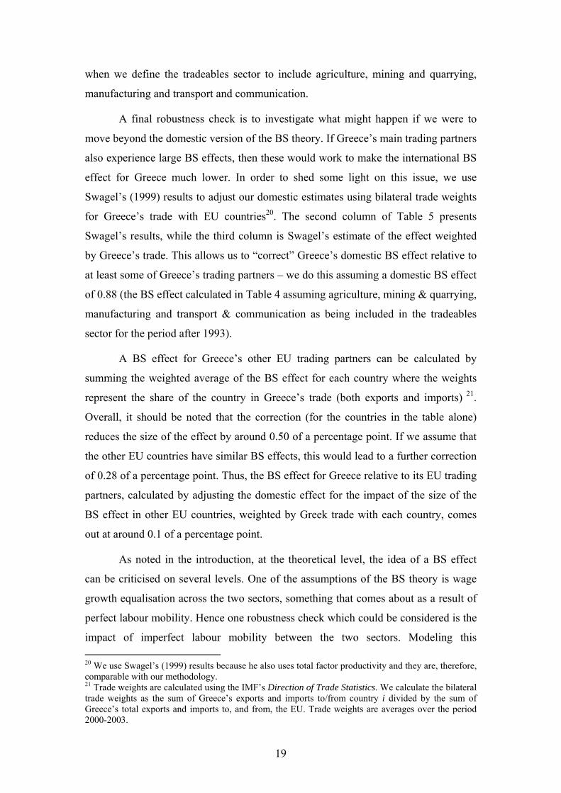
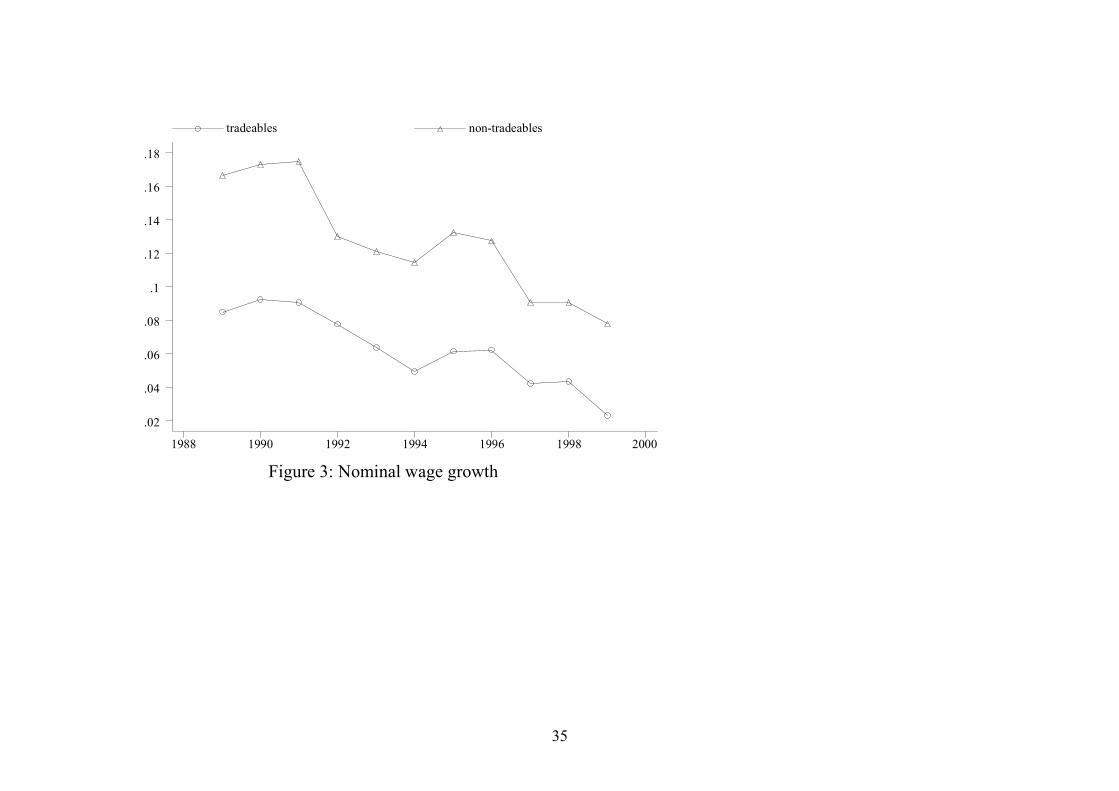
Figure 3 shows nominal wage growth (to the extent that the data allows us to

create tradeables and non-tradeables wage growth16). It indicates that wage growth in

the non-tradeables sector was consistently higher than that in the tradeables sector.

This observation is at odds with the BS assumption of wage growth equalisation

across sectors. We return to this matter later.

3.3 Results

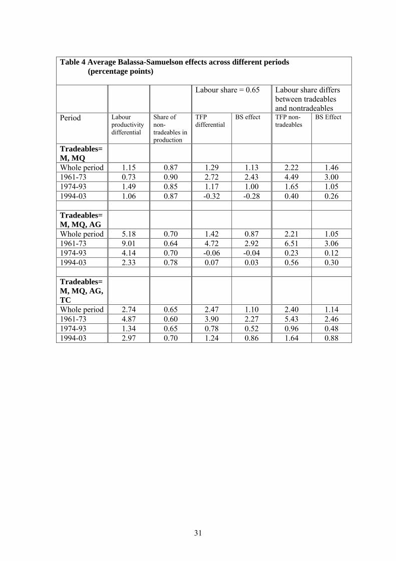
Table 4 reports labour productivity differentials along with TFP differentials

produced using the two different assumptions about labour shares. As noted above,

the use of TFP growth differentials, rather than labour productivity differentials, can

lead to estimates that differ quite significantly. Table 4 also provides estimates of the

average Balassa-Samuelson effect for the various definitions of both the tradeables

sectors and for the two labour share assumptions. Aside from an average for the

whole period, the three sub-periods identified above are also included.

Whilst for the whole period, the BS effect varies between 1 and 1.5 percentage

points, a result that is similar to that of Swagel’s 1 percentage point for his data period

(1960-96), the differences across sub-periods makes this result less meaningful as an

estimate of the BS effect at any single point in time. In fact, the results for the sub-

periods suggest a strong effect of around 3 percentage points in the period before the

first oil price shock in 1973, a sharp decline from 1974 to 1993, followed by a slight

recovery thereafter. Thus, in the final sub-period, the BS effect in general lies well

below 1 percentage point, depending on the definition of the tradeables sector.

A disadvantage of averaging over given periods is that we may implicitly

assume breaks in the series when, in fact, they do not occur. One way of dealing with

this potential problem is to estimate the BS effect using moving averages calculated

on the raw data17. This procedure allows different sub-periods to emerge more clearly

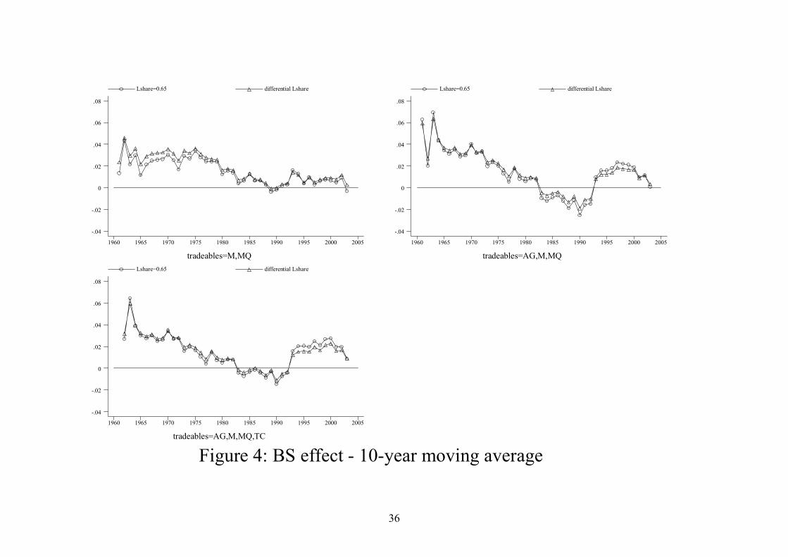
from the data. Figure 4 presents the results for the 10-year moving average series

across the different assumptions about what is included in the 16 Tradeables wage growth is average blue-collar hourly wage growth in manufacturing and mining & quarrying weighted by the shares of gross value added in each sector. Non-tradeables wage growth is average rates of growth of monthly wages in retail trade, banks and insurance as well as the hourly minimum wage for blue-collar workers. The results are robust to other definitions of the two sectors. We choose to present the results in Figure 3 because these measures generate the longest period of data. 17 We take 5 or 10-year moving averages of output growth, labour force growth, capital stock growth and the share of nontradeables in total production and then calculate TFP growth rates and the BS effect itself.

17

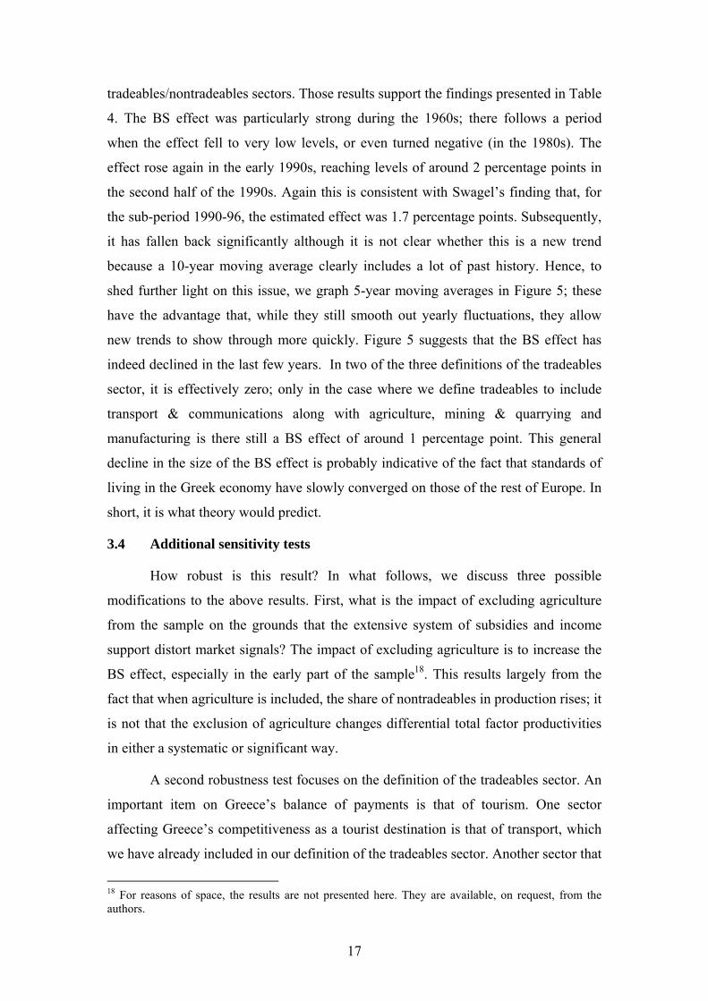
tradeables/nontradeables sectors. Those results support the findings presented in Table

4. The BS effect was particularly strong during the 1960s; there follows a period

when the effect fell to very low levels, or even turned negative (in the 1980s). The

effect rose again in the early 1990s, reaching levels of around 2 percentage points in

the second half of the 1990s. Again this is consistent with Swagel’s finding that, for

the sub-period 1990-96, the estimated effect was 1.7 percentage points. Subsequently,

it has fallen back significantly although it is not clear whether this is a new trend

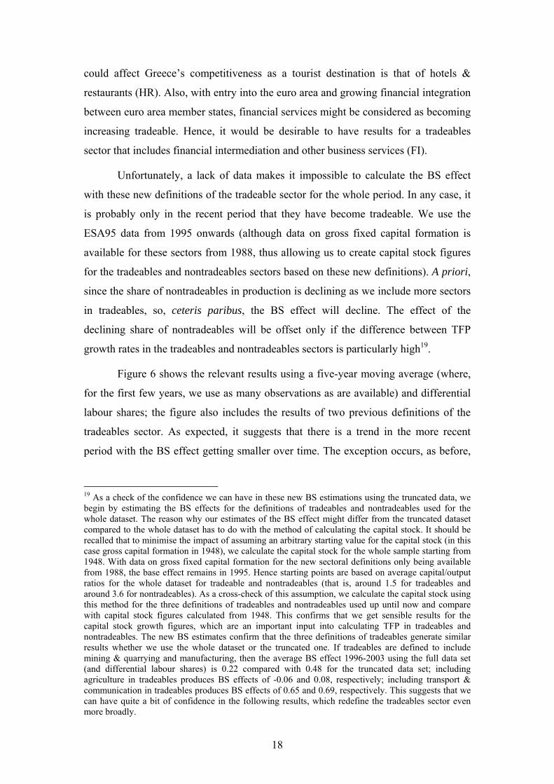
because a 10-year moving average clearly includes a lot of past history. Hence, to

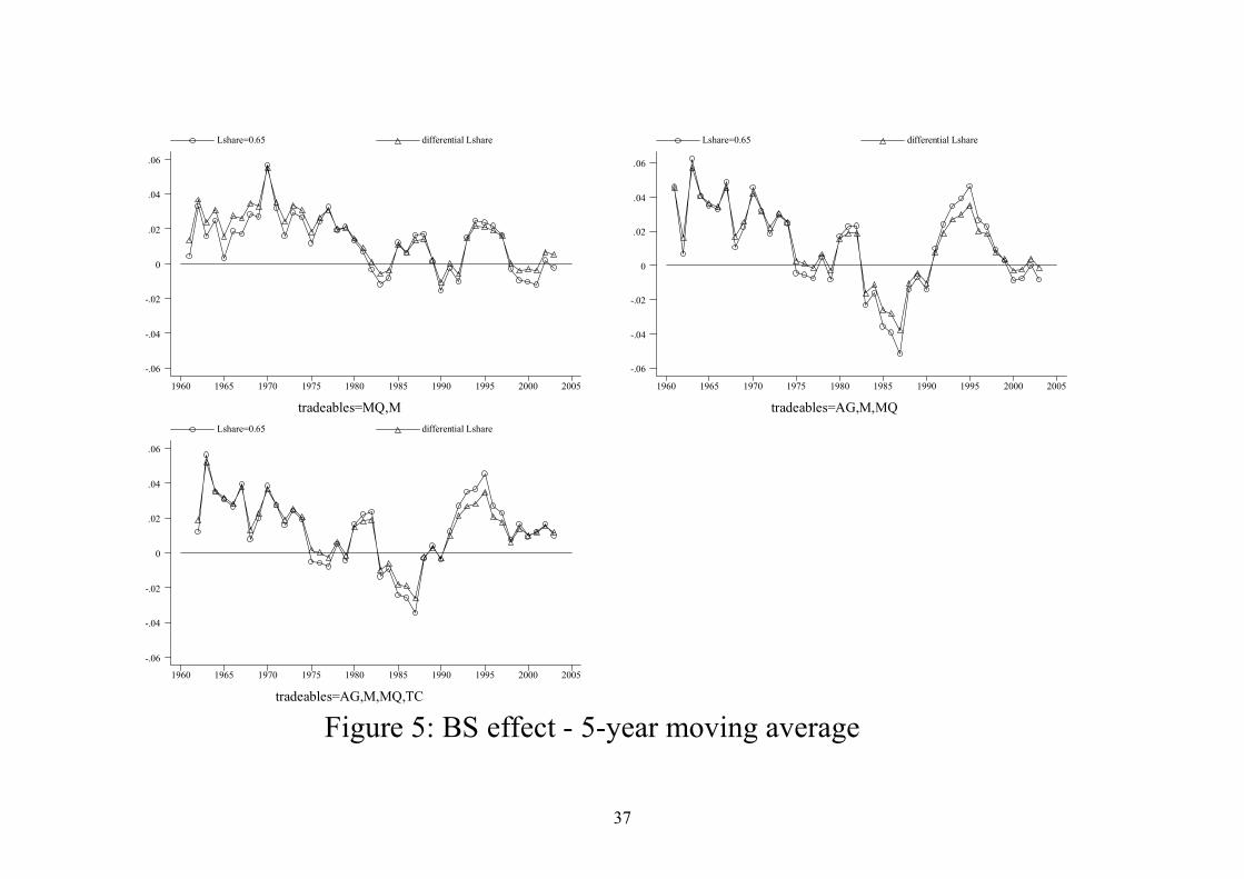
shed further light on this issue, we graph 5-year moving averages in Figure 5; these

have the advantage that, while they still smooth out yearly fluctuations, they allow

new trends to show through more quickly. Figure 5 suggests that the BS effect has

indeed declined in the last few years. In two of the three definitions of the tradeables

sector, it is effectively zero; only in the case where we define tradeables to include

transport & communications along with agriculture, mining & quarrying and

manufacturing is there still a BS effect of around 1 percentage point. This general

decline in the size of the BS effect is probably indicative of the fact that standards of

living in the Greek economy have slowly converged on those of the rest of Europe. In

short, it is what theory would predict.

3.4 Additional sensitivity tests

How robust is this result? In what follows, we discuss three possible

modifications to the above results. First, what is the impact of excluding agriculture

from the sample on the grounds that the extensive system of subsidies and income

support distort market signals? The impact of excluding agriculture is to increase the

BS effect, especially in the early part of the sample18. This results largely from the

fact that when agriculture is included, the share of nontradeables in production rises; it

is not that the exclusion of agriculture changes differential total factor productivities

in either a systematic or significant way.

A second robustness test focuses on the definition of the tradeables sector. An

important item on Greece’s balance of payments is that of tourism. One sector

affecting Greece’s competitiveness as a tourist destination is that of transport, which

we have already included in our definition of the tradeables sector. Another sector that

18 For reasons of space, the results are not presented here. They are available, on request, from the authors.

18

could affect Greece’s competitiveness as a tourist destination is that of hotels &

restaurants (HR). Also, with entry into the euro area and growing financial integration

between euro area member states, financial services might be considered as becoming

increasing tradeable. Hence, it would be desirable to have results for a tradeables

sector that includes financial intermediation and other business services (FI).

Unfortunately, a lack of data makes it impossible to calculate the BS effect

with these new definitions of the tradeable sector for the whole period. In any case, it

is probably only in the recent period that they have become tradeable. We use the

ESA95 data from 1995 onwards (although data on gross fixed capital formation is

available for these sectors from 1988, thus allowing us to create capital stock figures

for the tradeables and nontradeables sectors based on these new definitions). A priori,

since the share of nontradeables in production is declining as we include more sectors

in tradeables, so, ceteris paribus, the BS effect will decline. The effect of the

declining share of nontradeables will be offset only if the difference between TFP

growth rates in the tradeables and nontradeables sectors is particularly high19.

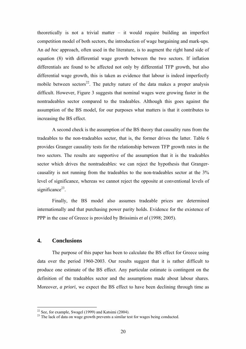
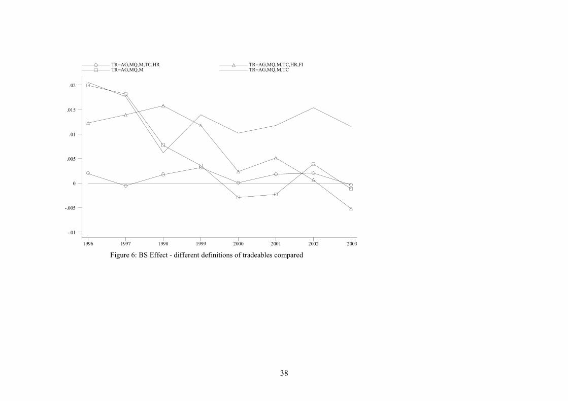
Figure 6 shows the relevant results using a five-year moving average (where,

for the first few years, we use as many observations as are available) and differential

labour shares; the figure also includes the results of two previous definitions of the

tradeables sector. As expected, it suggests that there is a trend in the more recent

period with the BS effect getting smaller over time. The exception occurs, as before,

19 As a check of the confidence we can have in these new BS estimations using the truncated data, we begin by estimating the BS effects for the definitions of tradeables and nontradeables used for the whole dataset. The reason why our estimates of the BS effect might differ from the truncated dataset compared to the whole dataset has to do with the method of calculating the capital stock. It should be recalled that to minimise the impact of assuming an arbitrary starting value for the capital stock (in this case gross capital formation in 1948), we calculate the capital stock for the whole sample starting from 1948. With data on gross fixed capital formation for the new sectoral definitions only being available from 1988, the base effect remains in 1995. Hence starting points are based on average capital/output ratios for the whole dataset for tradeable and nontradeables (that is, around 1.5 for tradeables and around 3.6 for nontradeables). As a cross-check of this assumption, we calculate the capital stock using this method for the three definitions of tradeables and nontradeables used up until now and compare with capital stock figures calculated from 1948. This confirms that we get sensible results for the capital stock growth figures, which are an important input into calculating TFP in tradeables and nontradeables. The new BS estimates confirm that the three definitions of tradeables generate similar results whether we use the whole dataset or the truncated one. If tradeables are defined to include mining & quarrying and manufacturing, then the average BS effect 1996-2003 using the full data set (and differential labour shares) is 0.22 compared with 0.48 for the truncated data set; including agriculture in tradeables produces BS effects of -0.06 and 0.08, respectively; including transport & communication in tradeables produces BS effects of 0.65 and 0.69, respectively. This suggests that we can have quite a bit of confidence in the following results, which redefine the tradeables sector even more broadly.

19

when we define the tradeables sector to include agriculture, mining and quarrying,

manufacturing and transport and communication.

A final robustness check is to investigate what might happen if we were to

move beyond the domestic version of the BS theory. If Greece’s main trading partners

also experience large BS effects, then these would work to make the international BS

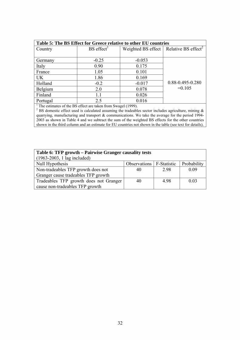
effect for Greece much lower. In order to shed some light on this issue, we use

Swagel’s (1999) results to adjust our domestic estimates using bilateral trade weights

for Greece’s trade with EU countries20. The second column of Table 5 presents

Swagel’s results, while the third column is Swagel’s estimate of the effect weighted

by Greece’s trade. This allows us to “correct” Greece’s domestic BS effect relative to

at least some of Greece’s trading partners – we do this assuming a domestic BS effect

of 0.88 (the BS effect calculated in Table 4 assuming agriculture, mining & quarrying,

manufacturing and transport & communication as being included in the tradeables

sector for the period after 1993).

A BS effect for Greece’s other EU trading partners can be calculated by

summing the weighted average of the BS effect for each country where the weights

represent the share of the country in Greece’s trade (both exports and imports) 21.

Overall, it should be noted that the correction (for the countries in the table alone)

reduces the size of the effect by around 0.50 of a percentage point. If we assume that

the other EU countries have similar BS effects, this would lead to a further correction

of 0.28 of a percentage point. Thus, the BS effect for Greece relative to its EU trading

partners, calculated by adjusting the domestic effect for the impact of the size of the

BS effect in other EU countries, weighted by Greek trade with each country, comes

out at around 0.1 of a percentage point.

As noted in the introduction, at the theoretical level, the idea of a BS effect

can be criticised on several levels. One of the assumptions of the BS theory is wage

growth equalisation across the two sectors, something that comes about as a result of

perfect labour mobility. Hence one robustness check which could be considered is the

impact of imperfect labour mobility between the two sectors. Modeling this 20 We use Swagel’s (1999) results because he also uses total factor productivity and they are, therefore, comparable with our methodology. 21 Trade weights are calculated using the IMF’s Direction of Trade Statistics. We calculate the bilateral trade weights as the sum of Greece’s exports and imports to/from country i divided by the sum of Greece’s total exports and imports to, and from, the EU. Trade weights are averages over the period 2000-2003.

20

theoretically is not a trivial matter – it would require building an imperfect

competition model of both sectors, the introduction of wage bargaining and mark-ups.

An ad hoc approach, often used in the literature, is to augment the right hand side of

equation (8) with differential wage growth between the two sectors. If inflation

differentials are found to be affected not only by differential TFP growth, but also

differential wage growth, this is taken as evidence that labour is indeed imperfectly

mobile between sectors22. The patchy nature of the data makes a proper analysis

difficult. However, Figure 3 suggests that nominal wages were growing faster in the

nontradeables sector compared to the tradeables. Although this goes against the

assumption of the BS model, for our purposes what matters is that it contributes to

increasing the BS effect.

A second check is the assumption of the BS theory that causality runs from the

tradeables to the non-tradeables sector, that is, the former drives the latter. Table 6

provides Granger causality tests for the relationship between TFP growth rates in the

two sectors. The results are supportive of the assumption that it is the tradeables

sector which drives the nontradeables: we can reject the hypothesis that Granger-

causality is not running from the tradeables to the non-tradeables sector at the 3%

level of significance, whereas we cannot reject the opposite at conventional levels of

significance23.

Finally, the BS model also assumes tradeable prices are determined

internationally and that purchasing power parity holds. Evidence for the existence of

PPP in the case of Greece is provided by Brissimis et al (1998; 2005).

4. Conclusions

The purpose of this paper has been to calculate the BS effect for Greece using

data over the period 1960-2003. Our results suggest that it is rather difficult to

produce one estimate of the BS effect. Any particular estimate is contingent on the

definition of the tradeables sector and the assumptions made about labour shares.

Moreover, a priori, we expect the BS effect to have been declining through time as

22 See, for example, Swagel (1999) and Katsimi (2004). 23 The lack of data on wage growth prevents a similar test for wages being conducted.

21

catch-up occurs not only with respect to the rest of the world, but also as the non-

tradeables sector within Greece catches up with the tradeables.

In the light of these difficulties, the approach we have taken has been to

present a variety of results with an emphasis on their robustness. One strong

conclusion that emerges has been to confirm that the size of the BS effect has not

been constant throughout the whole period. During the 1960s, when catch-up was

particularly strong, estimates show a quite significant BS effect (around 3 percentage

points); this effect, however, almost disappears, falling to around 0-0.5 of a

percentage point during the period of stagnation between the late 1970s and the early

1990s, before picking up again in the second phase of catch-up during the 1990s.

Thus, to present an estimate of the effect based on an average over the whole period

would be misleading. At the same time, factors such as the effects of the business

cycle on productivity measurements suggest that we have to be very careful when

looking at annual estimates of the BS effect. Rather there is a need to average at least

across the cycle. This suggests that a moving average estimate is more appropriate.

What moving average estimates tend on balance to show for the recent period

is that the BS effect, whilst quite significant in the second half of the 1990s (around 1-

2 percentage points, in line with Swagel’s estimates), has been declining to around 0.5

of a percentage point in recent years. Such a result is not inconsistent with our priors.

Since joining the euro area, the average differential inflation between Greece and the

euro area has been 1.27 percentage points. The estimates provided here suggest that,

at best, only about one-fifth of that differential can be accounted for by the Balassa-

Samuelson effect.

22

References Alberola-Ila E and T. Tyrvainen (1998), “Is there Scope for Inflation Differentials in

EMU?”, Banco de Espana, Working Paper, no. 9823.

Arratibel, O., D. Rodriguez-Palenzuela and C. Thimann (2002), “Inflation Dynamics and Dual Inflation in Accession Countries: A “New-Keynesian” Perspective”, ECB Working Paper, no. 132.

Balassa, B. (1964), “The Purchasing Power Parity Doctrine: A Reappraisal”, Journal of Political Economy, 72, 584-96.

Baumol, W. and W. Bowen (1966), Performing Arts: The Economic Dilemma, New York, 20th Century Fund.

Bragoudakis, Z. and D. Moschos (2000), “Relative Prices and Sectoral Labor Differentials: A Long-Run Analysis for Greece”, Ekonomia, 4, 2, 142-55.

Brissimis, S., D. Sideris and F. Voumvaki (1998), “Purchasing Power Parity as a Long-Run Relationship: An Empirical Investigation of the Greek Case”, Bank of Greece Economic Bulletin, 12, 21-54

Brissimis, S., D. Sideris and F. Voumvaki (2005), “Testing Long-Run Purchasing Power Parity under Exchange Rate Targeting”, Journal of International Money and Finance, 24, 6, 959-81

Canzoneri, M., R. Cumby, B. Diba and G. Eudey (2002), “Productivity Trends in Europe: Implications for Real Exchange Rates, Real Interest Rates and Inflation”, Review of International Economics, 10, 3, 497-516.

Crespo-Cuaresma, J., J. Fidrmuc and R. MacDonald (2005), “The Monetary Approach to Exchange Rates in the CEECs”, Economics of Transition, 13, 2, 395-416.

De Broeck, M. and T. Slok (2001), “Interpreting Real Exchange Rate Movements in Transition Countries”, IMF Working Paper, WP/01/56.

Doyle, P., L. Kuijs and G. Jiang (2001), “Real Convergence to EU Income Levels: Central Europe from 1990 to the Long Term”, IMF Working Paper, WP/01/146.

Drine, I. and C. Rault (2003), “Do Panel Data Permit the Rescue of the Balassa-Samuelson Effect for Latin American Countries?, Applied Economics, 35, 351-59.

Drine, I. and C. Rault (2005), “Can the Balassa-Samuelson Effect Explain Long-Run Exchange Rate Movements in OECD Countries?, Applied Financial Economics, 15, 519-30.

ECB (2003), Inflation Differentials in the Euro Area: Potential Causes and Policy Implications, ECB, Frankfurt.

Egert, B., L. Halpern and R. MacDonald (2006), “Equilibrium Exchange Rates in Transition Economies: Taking Stock of the Issues”, Journal of Economic Surveys, 20, 257-324.

Faria, J. R. and L. Leon-Ledesma (2000), “Testing the Balassa-Samuelson Effect: Implications for Growth and PPP”, University of Kent, Discussion Papers in Economics, 00/08.

23

Fischer, C. (2002), “Real Currency Appreciation in Accession Countries: Balassa-Samuelson and Investment Demand”, Deutsche Bundesbank, Discussion Paper, 19/02.

Flek, V., L. Markova and J. Podpiera (2002), “Sectoral Productivity and Real Exchange Rate Appreciation: Much Ado about Nothing?”, Czech National Bank, Working Paper Series, 4.

Froot, K. and K. Rogoff (1995), “Perspectives on PPP and Long-Run Real Exchange Rates”, Ch. 32 in Handbook of International Economics, Vol III (ed) G. Grossman and K. Rogoff, Elsevier: Amsterdam.

Ito, T., P. Isard and S. Symansky (1997), “Economic Growth and Real Exchange Rate: An Overview of the Balassa-Samuelson Hypothesis in Asia”, NBER Working Paper, no. 5979.

Katsimi, M. (2004), “Inflation Divergence in the Euro Area: The Balassa-Samuelson Effect”, Applied Economics Letters, 11, 329-332.

Lommatzsch, K. and S. Tober (2006), “Euro-Area Inflation: Does the Balassa-Samuelson Effect Matter? International Economics and Economic Policy, 3, 2, 105-136.

Lunnemann, P. and T. Y. Matha (2005), “Regulated and Service Prices and Inflation Persistence”, European Central Bank, Working Paper no. 466.

Malley, J. (2006), “The Theory and Estimation of the Balassa-Samuelson Effect: Some Background Notes”, mimeo.

Mihaljek, D. and M. Klau (2003), “The Balassa-Samuelson Effect in Central Europe: A Disaggregated Analysis”, BIS Working Paper, no. 143.

Obstfeld, M. and K. Rogoff (1996), Foundations of International Macroeconomics, MIT Press.

Ortega, E. (2003), “Persistent Inflation Differentials in Europe”, Banco de Espana Working Paper no. 0305.

Samuelson, P. (1964), “Theoretical Notes on Trade Problems”, Review of Economics and Statistics, 46, 145-54.

Sinn, H.-W. and M. Reutter (2001), “The Minimum Inflation Rate for Euroland”, NBER Working Paper No. 8085.

Swagel P (1999), “The Contribution of the Balassa-Samuelson Effect to Inflation: Cross-Country Evidence”, IMF Staff Country Report, no.99/138.

Timmer, M. and M. O’Mahony (undated) “Measuring Capital Input”, EPKE Technical Note No. 1, National Institute of Economic and Social Research, available at http://www.niesr.ac.uk/research/epke/working_papers.html

24

Data appendix

The data was compiled using sectoral national accounts data for Greece from 1948 to

2003. The major problem associated with the data compilation was the many changes

in the system of recording national account aggregates, especially at the sectoral level.

Whilst, the National Statistical Service of Greece has produced national account

aggregates for the whole economy using ESA95 going back to the 1960s, the sectoral

information provided is strictly limited. Aside from the fact that new systems of

national accounting entail different ways of counting the various aggregates, there is

also the problem that sectoral definitions change. In this appendix we provide details

on how the database was constructed. Table A1 defines the two sectors, tradeables

and non-tradeables in terms of the classification scheme used in each of the national

accounts systems.

Output is measured by Gross Value Added (GVA). The database contains both

current and constant (1995) prices GVA. We started with the figures for 1995-2003

(based on ESA95) to calculate the broad sectors of agriculture, industry (including

construction), mining and quarrying, manufacturing and services. Figures are then

backdated using the EU’s AMECO database for 1960-94 (by using rates of change).

AMECO does not contain information on mining and quarrying and hence figures are

backdated to 1988 using rates of change of GVA in mining and quarrying from

National Accounts (ESA79) and to 1960 using rates of change of GDP in mining and

quarrying from the revised National Accounts 1960-97 (ESA79)

Gross Fixed Capital formation data (both current and constant 1995 prices) on

a sectoral basis is still only available from 1995 to 1998 on a sectoral level from the

published national accounts (ESA95). Data was therefore taken from the OECD’s

STAN Sectoral Database for 1995 to 2003. We then backdated using rates of change

to 1989 from National Accounts data (ESA79) and to 1948 with National Accounts

data (ESA70). Data was collected from 1948 in order to help eliminate base year

effects when calculating the capital stock using the perpetual inventory method where

depreciation is assumed to be 10% per annum in the traded goods sector and 4% in

the nontraded sector.

For employment data, we again begin with the ESA95 data as this is more

complete, using as it does not only the labour force survey, but also other sources of

25

information (eg better data for agriculture than was used in the past). Using this data

we calculate the following broad groups: agriculture, industry (plus construction),

manufacturing, mining and quarrying and services. We then backdate using growth

rates for theses broad aggregates using OECD data on rates of change of civilian

employment. For mining and quarrying (where OECD data is unavailable), we also

use census data for the earlier period of the 1960s and 1970s and Labour Force

Survey data for the 1980s (Labour Force Survey data for the period before 1981

covered the Athens area only).

The tradeables sector is defined in two ways in the paper. First, we include

manufacturing along with mining and quarrying, leaving agriculture, industry (minus

manufacturing and mining and quarrying) and services as non-tradeables. Second, we

test the sensitivity of these results to redefining tradeables to include agriculture.

Finally, for prices we use sectoral CPI rates. Pre-1990 there were 9 categories

which were subsequently extended to 12 categories. The categories were combined

(as detailed in Table A2) to generate measures of traded and nontraded sectors as

defined in the main text using the appropriate weights. When we include agriculture

as a tradeable, food and non-alcoholic beverage and alcohol and tobacco are included

in tradeables.

26

Table A1 National Accounts Categories

Broad sectors (definitions used below)

Sectors published in National Accounts

ESA 95 Non-tradeables Agriculture Agriculture &fishing

Industry (excl. manufacturing) Electricity etc

Construction Services Wholesale/retail trade Hotels &restaurants Transport &communications

Financial intermediation, real

estate Other services (mainly public) Tradeables Mining &quarrying Manufacturing ESA 79, ESA 70 Non-tradeables Agriculture Agriculture

Industry (excl. manufacturing) Electricity etc

Transport & communication Construction Services Public Administration Dwellings Other services Tradeables Mining & quarrying Manufacturing

27

Table A2 Sectoral Breakdown of the Consumer Price Index 1960-89 Non-tradeables food and non-alcoholic beverages alcohol and tobacco housing health education and recreation transport and communications other services food and non-alcoholic beverages Tradeables clothing and footwear consumer durables 1989-2003 Non-tradeables alcohol and tobacco housing health transport communications recreation and cultural activities education hotels and restaurants other services Tradeables consumer durables clothing and footwear

28

Table 1: Definition of tradeables/nontradeables sectors

Tradeables Nontradeables Data Availability

Mining & quarrying Manufacturing

Agriculture, services 1960-2003

Agriculture Mining & quarrying Manufacturing

Services 1960-2003

Agriculture Mining & quarrying Manufacturing Transport & Communications

Services excluding: Transport & Communications

1960-2003

Agriculture Mining & quarrying Manufacturing Transport & Communications Hotels & Restaurants

Services excluding: Transport & Communications Hotels & Restaurants

1995-2003

Agriculture Mining & quarrying Manufacturing Transport & Communications Hotels & Restaurants Financial Intermediation, Real Estate & Other Business Services

Services excluding: Transport & Communications Hotels & Restaurants Financial Intermediation, Real Estate & Other Business Services

1995-2003

29

Table 2: Relative productivity growth (%) Labour productivity growth

TR=MQ,M TR=AG,MQ,M TR=AG,MQ,M,TCWhole period Tradeables 4.65 6.73 4.41 Non-tradeables 3.50 1.55 1.67 1961-1973 Tradeables 9.55 14.41 10.21 Non-tradeables 8.82 5.40 5.34 1974-1993 Tradeables 2.08 3.19 1.00 Non-tradeables 0.59 -0.95 -0.34 1994-2003 Tradeables 3.44 3.84 4.27 Non-tradeables 2.38 1.51 1.30 Total factor productivity growth

TR=MQ,M TR=AG,MQ,M TR=AG,MQ,M,TCWhole period Tradeables 3.59 2.98 2.85 Non-tradeables 1.37 0.77 0.45 1961-1973 Tradeables 8.40 8.45 7.19 Non-tradeables 3.91 1.94 1.76 1974-1993 Tradeables 1.29 -0.00 0.40 Non-tradeables -0.36 -0.23 -0.56 1994-2003 Tradeables 1.92 1.82 2.54 Non-tradeables 1.52 1.26 0.90 Memorandum item: average per annum real GDP growth rate Whole period 1961-73 1974-93 1994-2003 4.04 8.59 1.51 3.38

30

Table 3: Labour shares across tradeables and nontradeables (averages 1995-2003) Labour share Definition of tradeables Tradeables Nontradeables TR = MQ, M 0.74 0.56 TR = AG, MQ, M 0.73 0.55 TR = AG, MQ, M, TC 0.70 0.54

31

Table 4 Average Balassa-Samuelson effects across different periods (percentage points) Labour share = 0.65 Labour share differs

between tradeables and nontradeables

Period Labour productivity differential

Share of non-tradeables in production

TFP differential

BS effect TFP non-tradeables

BS Effect

Tradeables=M, MQ

Whole period 1.15 0.87 1.29 1.13 2.22 1.46 1961-73 0.73 0.90 2.72 2.43 4.49 3.00 1974-93 1.49 0.85 1.17 1.00 1.65 1.05 1994-03 1.06 0.87 -0.32 -0.28 0.40 0.26 Tradeables=M, MQ, AG

Whole period 5.18 0.70 1.42 0.87 2.21 1.05 1961-73 9.01 0.64 4.72 2.92 6.51 3.06 1974-93 4.14 0.70 -0.06 -0.04 0.23 0.12 1994-03 2.33 0.78 0.07 0.03 0.56 0.30 Tradeables=M, MQ, AG, TC

Whole period 2.74 0.65 2.47 1.10 2.40 1.14 1961-73 4.87 0.60 3.90 2.27 5.43 2.46 1974-93 1.34 0.65 0.78 0.52 0.96 0.48 1994-03 2.97 0.70 1.24 0.86 1.64 0.88

32

Table 5: The BS Effect for Greece relative to other EU countries Country

BS effect1 Weighted BS effect Relative BS effect2

Germany -0.25 -0.053 Italy 0.90 0.175 France 1.05 0.101 UK 1.86 0.169 Holland -0.2 -0.017 Belgium 2.0 0.078 Finland 1.1 0.026 Portugal 2.5 0.016

0.88-0.495-0.280 =0.105

1 The estimates of the BS effect are taken from Swagel (1999). 2 BS domestic effect used is calculated assuming the tradeables sector includes agriculture, mining & quarrying, manufacturing and transport & communications. We take the average for the period 1994-2003 as shown in Table 4 and we subtract the sum of the weighted BS effects for the other countries shown in the third column and an estimate for EU countries not shown in the table (see text for details).

Table 6: TFP growth – Pairwise Granger causality tests (1963-2003, 1 lag included) Null Hypothesis Observations F-Statistic Probability Non-tradeables TFP growth does not Granger cause tradeables TFP growth

40 2.98 0.09

Tradeables TFP growth does not Granger cause non-tradeables TFP growth

40 4.98 0.03

33

Figure 1: Greece: total factor productivity growth (left-hand axis) and per capita GDP at PPP exchange rates relative to EU15/OECD (right-hand axis)

-0.02

-0.01

0

0.01

0.02

0.03

0.04

0.05

0.06

0.07

0.08

1960 1965 1970 1975 1980 1985 1990 1995 2000 2005

30

35

40

45

50

55

60

65

70

75

80

85

TFP growth (5-year moving average) GDP per capita (relative to EU15)GDP per capita volume index (relative to OECD)

Note: There is a break in the series of per capita GDP relative to the EU15 in 1970.

34

Figure 2: Relative Prices & Productivity - nontradeables/tradeables

rela

tive

pric

es

Tradeables=MQ,M

1960 1965 1970 1975 1980 1985 1990 1995 2000

.8

.9

1

1.1

rela

tive

pric

es

Tradeables=AG,MQ,M

1960 1965 1970 1975 1980 1985 1990 1995 2000

.86

.88

.9

.92

.94

.96

.98

1

1.02

rela

tive

pric

es

Tradeables=AG,MQ,M,TC

1960 1965 1970 1975 1980 1985 1990 1995 2000

.8

.9

1

1.1

rela

tive

prod

uctiv

ity

Tradeables=MQ,M

1960 1965 1970 1975 1980 1985 1990 1995 2000

1.02

1.04

1.06

1.08

1.1

rela

tive

prod

uctiv

ity

Tradeables=AG,MQ,M

1960 1965 1970 1975 1980 1985 1990 1995 2000

1.1

1.2

1.3

1.4

1.5

1.6

1.7

rela

tive

prod

uctiv

ity

Tradeables=AG,MQ,M,TC

1960 1965 1970 1975 1980 1985 1990 1995 2000

1

1.05

1.1

1.15

1.2

35

Figure 3: Nominal wage growth

tradeables non-tradeables

1988 1990 1992 1994 1996 1998 2000

.02

.04

.06

.08

.1

.12

.14

.16

.18

36

Figure 4: BS effect - 10-year moving average

tradeables=M,MQ

Lshare=0.65 differential Lshare

1960 1965 1970 1975 1980 1985 1990 1995 2000 2005

-.04

-.02

0

.02

.04

.06

.08

tradeables=AG,M,MQ

Lshare=0.65 differential Lshare

1960 1965 1970 1975 1980 1985 1990 1995 2000 2005

-.04

-.02

0

.02

.04

.06

.08

tradeables=AG,M,MQ,TC

Lshare=0.65 differential Lshare

1960 1965 1970 1975 1980 1985 1990 1995 2000 2005

-.04

-.02

0

.02

.04

.06

.08

37

Figure 5: BS effect - 5-year moving average

tradeables=MQ,M

Lshare=0.65 differential Lshare

1960 1965 1970 1975 1980 1985 1990 1995 2000 2005

-.06

-.04

-.02

0

.02

.04

.06

tradeables=AG,M,MQ

Lshare=0.65 differential Lshare

1960 1965 1970 1975 1980 1985 1990 1995 2000 2005

-.06

-.04

-.02

0

.02

.04

.06

tradeables=AG,M,MQ,TC

Lshare=0.65 differential Lshare

1960 1965 1970 1975 1980 1985 1990 1995 2000 2005

-.06

-.04

-.02

0

.02

.04

.06

38

Figure 6: BS Effect - different definitions of tradeables compared

TR=AG,MQ,M,TC,HR TR=AG,MQ,M,TC,HR,FI TR=AG,MQ,M TR=AG,MQ,M,TC

1996 1997 1998 1999 2000 2001 2002 2003

-.01

-.005

0

.005

.01

.015

.02

39

BANK OF GREECE WORKING PAPERS 41. Genberg, H., “Exchange-Rate Arrangements and Financial Integration in East

Asia: On a Collision Course?”, including comments by James A. Dorn and Eiji Ogawa, May 2006.

42.Christl, J., “Regional Currency Arrangements: Insights from Europe”, including

comments by Lars Jonung and the concluding remarks and main findings of the workshop by Eduard Hochreiter and George Tavlas, June 2006.

43.Edwards, S., “Monetary Unions, External Shocks and Economic Performance: A

Latin American Perspective”, including comments by Enrique Alberola, June 2006.

44.Cooper, R. N., “Proposal for a Common Currency Among Rich Democracies” and

Bordo, M. and H. James, “One World Money, Then and Now”, including comments by Sergio L. Schmukler, June 2006.

45.Williamson, J., “A Worldwide System of Reference Rates”, including comments

by Marc Flandreau, August 2006. 46.Brissimis, S. N., M. D. Delis and E. G. Tsionas, “Technical and Allocative

Efficiency in European Banking”, September 2006. 47.Athanasoglou, P. P., M. D. Delis and C. K. Staikouras, “Determinants of Bank

Profitability in the South Eastern European Region”, September 2006. 48.Petroulas, P., “The Effect of the Euro on Foreign Direct Investment”, October

2006. 49.Andreou, A. S. and G. A. Zombanakis, “Computational Intelligence in Exchange-

Rate Forecasting”, November 2006. 50.Milionis, A. E., “An Alternative Definition of Market Efficiency and Some

Comments on its Empirical Testing”, November 2006. 51.Brissimis, S. N. and T. S. Kosma, “Market Conduct, Price Interdependence and

Exchange Rate Pass-Through”, December 2006. 52.Anastasatos, T. G. and I. R. Davidson, “How Homogenous are Currency Crises?

A Panel Study Using Multiple Response Models”, December, 2006. 53.Angelopoulou, E. and H. D. Gibson, “The Balance Sheet Channel of Monetary

Policy Transmission: Evidence from the UK”, January, 2007. 54.Brissimis, S. N. and M. D. Delis, “Identification of a Loan Supply Function: A

Cross-Country Test for the Existence of a Bank Lending Channel”, January, 2007.

40

55.Angelopoulou, E., “The Narrative Approach for the Identification of Monetary Policy Shocks in a Small Open Economy”, February, 2007.

56.Sideris, D. A., “Foreign Exchange Intervention and Equilibrium Real Exchange

Rates”, February 2007. 57.Hondroyiannis, G., P.A.V.B. Swamy and G. S. Tavlas, “The New Keynesian

Phillips Curve and Lagged Inflation: A Case of Spurious Correlation?”, March 2007.

58.Brissimis, S. N. and T. Vlassopoulos, “The Interaction between Mortgage

Financing and Housing Prices in Greece”, March 2007. 59.Mylonidis, N. and D. Sideris, “Home Bias and Purchasing Power Parity: Evidence

from the G-7 Countries”, April 2007. 60. Petroulas, P., “Short-Term Capital Flows and Growth in Developed and

Emerging Markets”, May 2007. 61.Hall, S. G., G. Hondroyiannis, P.A.V.B. Swamy and G. S. Tavlas, “A Portfolio

Balance Approach to Euro-area Money Demand in a Time-Varying Environment”, October 2007.

62. Brissimis, S. N. and I. Skotida, “Optimal Monetary Policy in the Euro Area in the

Presence of Heterogeneity”, November 2007.