. Article .Progress of Projects Supported by NSFC

SCIENCE CHINAPhysics, Mechanics & Astronomy

December 2012 Vol. 55 No. 12: 2244–2258doi: 10.1007/s11433-012-4945-9

c! Science China Press and Springer-Verlag Berlin Heidelberg 2012 phys.scichina.com www.springerlink.com

Testing modified gravity models with recent cosmologicalobservations

ZHANG WenShuai1,2, CHENG Cheng2,3, HUANG QingGuo2,3,4*, LI Miao2,3,4, LI Song2,3,LI XiaoDong1,2,5 & WANG Shuang1,2

1Department of Modern Physics, University of Science and Technology of China, Hefei 230026, China;2Institute of Theoretical Physics, Chinese Academy of Sciences, Beijing 100190, China;

3Kavli Institute for Theoretical Physics China, Chinese Academy of Sciences, Beijing 100190, China;4State Key Laboratory of Theoretical Physics, Chinese Academy of Sciences, Beijing 100190, China;

5Interdisciplinary Center for Theoretical Study, University of Science and Technology of China, Hefei 230026, China

Received August 7, 2012; accepted October 17, 2012; published online November 16, 2012

We explore the cosmological implications of five modified gravity (MG) models by using the recent cosmological observationaldata, including the recently released SNLS3 type Ia supernovae sample, the cosmic microwave background anisotropy data from theWilkinson Microwave Anisotropy Probe 7-yr observations, the baryon acoustic oscillation results from the Sloan Digital Sky Surveydata release 7, and the latest Hubble constant measurement utilizing the Wide Field Camera 3 on the Hubble Space Telescope. TheMG models considered include the Dvali-Gabadadze-Porrati (DGP) model, two f (R) models, and two f (T ) models. We find thatcompared with the !CDM model, MG models can not lead to an appreciable reduction of the !2

min. The analysis of AIC and BICshows that the simplest cosmological constant model (!CDM) is still the most preferred by the current data, and the DGP modelis strongly disfavored. In addition, from the observational constraints, we also reconstruct the evolutions of the growth factor inthese models. We find that the current available growth factor data are not enough to distinguish these MG models from the !CDMmodel.

modified gravity, cosmic acceleration, dark energy experiment, growth factor

PACS number(s): 98.80.-k, 95.36.+x, 04.50.+h

Citation: Zhang W S, Cheng C, Huang Q G, et al. Testing modified gravity models with recent cosmological observations. Sci China-Phys Mech Astron, 2012,55: 2244–2258, doi: 10.1007/s11433-012-4945-9

1 Introduction

Since its discovery in 1998 [1], the cosmic acceleration hasbecome one of the central problems in theoretical physicsand cosmology. The most common approach to explainingthe cosmic acceleration is modifying the right hand side ofEinstein equation, i.e., introducing a mysterious compositioncalled dark energy (DE) [2]. Numerous theoretical DE mod-els have been proposed in the last decade [3–13], while it isstill as daunting as ever to understand the nature of the cosmicacceleration [14].

In addition to the introduction of the DE component,

*Corresponding author (email: huangqg@itp.ac.cn)

another popular route to explaining the cosmic acceleration,i.e., modifying the left hand side of Einstein equation, hasalso drawn considerable attention. They are the so-calledmodified gravity (MG) models [15, 16]. So far, a lot ofMG models have been proposed, providing various inter-esting mechanisms for the cosmic acceleration. For exam-ple, in the DGP braneworld model [17], gravity is altered atimmense distances by slow leakage of gravity o" from ourthree-dimensional universe, leading to the apparent accelera-tion in the cosmological scale. In the f (R) gravity [18, 19],the Ricci scalar R is generalized to a function f (R), provid-ing another possible mechanism for the cosmic acceleration.A similar idea is the f (T ) gravity [20–22], where the tor-sion T is replaced by a function f (T ). Other popular MG

Zhang W S, et al. Sci China-Phys Mech Astron December (2012) Vol. 55 No. 12 2245

models include MOND [23], TeVeS [24], Brans-Dicke grav-ity [25], Gauss-Bonnet gravity [26], Horava-Lifshitz grav-ity [27], and so on [28]. For recent reviews about MG models,see refs. [16, 29].

There are mainly two ways to constrain the cosmologicalmodels by using the observational data. First, they can betested through their e"ects in the cosmic expansion history,which can be measured through Type Ia supernoave (SNIa),baryon acoustic oscillations (BAO), and so on. Second, theycan be tested through their e"ects in the cosmic growth his-tory, which can be measured through the Integrated SachsWolfe (ISW) e"ect [30], weak lensing, galaxy clusters, andso on. So far, many studies have been performed [31–38].

In this work, we will mainly test the MG models againstthe observations of the cosmic expansion history. Recently, ahigh-quality joint sample of 472 supernovae (SN), the SNLS3SNIa dataset [39], was released. Moreover, the systematicuncertainties of the SNIa data were nicely handled in work[39]. It is interesting to study the performance of MG mod-els when confronted with this newly released SNIa dataset.Thus, in this work we will adopt SNLS3 dataset and sys-tematically study 5 representative MG models, including theDGP model, two f (R) models, and two f (T ) models. Toperform a comprehensive analysis, we also include the cos-mic microwave background (CMB) anisotropy data from theWilkinson Microwave Anisotropy Probe 7-yr (WMAP7) ob-servations [40], the BAO results from the Sloan Digital SkySurvey (SDSS) Data Release 7 (DR7) [41], and the latestHubble constant measurement from the Wide Field Camera 3(WFC3) on the HST [42]. Utilizing these data, we constrainthe parameter space of these MG models, and compare themwith the !CDM model by using the AIC [43] and BIC [44]criterion.

An important tool to study the cosmic growth history isgrowth factor [45]. However, compared with the cosmic ex-pansion history data, the current growth factor observationshave larger errors (Their redshifts are also not well deter-mined). Moreover, some data points of growth factor obser-vations are obtained by assuming !CDM, and therefore theiruse to test models di"erent from !CDM may not be reliable.So in this work we will not include the growth factor datawhen performing observational constraints on the MG mod-els. Instead, making use of the constraints on the MG modelsobtained from the observations of the cosmic expansion his-tory, we reconstruct the evolutions of the growth factor alongwith the redshift z in these models and compare the resultswith the growth factor data. In this way, we can see whetherit is possible to distinguish these MG models from the growthfactor data.

This paper is organized as follows: In sect. 2, we give abrief and overall description of the models considered here,as well as the analysis methods used. In sect. 3, we introducein detail the current observational data of the cosmic expan-sion history and the cosmic growth history, respectively. Insect. 4, we study the cosmological interpretations of the MGmodels considered here and summarize the comparisons of

the models. In sect. 5, we give a short discussion. In ad-dition, we present two appendice about the initial conditionof evolution equation of growth factor and the e"ects of theparameter n in f (R) model. In this work, we assume today’sscale factor a0 = 1, so the redshift z = a"1 " 1; the subscript“0” always indicates the present value of the correspondingquantity, and the unit with c = ! = 1 is used.

2 Models and methodology

2.1 Models

In this work, we will investigate five representative MG mod-els, including

(1) the DGP model;(2) a power-law type f (T ) model ( f (T )PL);(3) an exponential type f (T ) model ( f (T )EXP);(4) the f (R) model proposed by Starobinsky ( f (R)St);(5) the f (R) model proposed by Hu and Sawicki ( f (R)HS).The DGP model is a braneworld model [17], where grav-

ity is altered at immense distances by slow leakage of gravityo" from our three-dimensional universe. In the f (T ) mod-els, the torsion T in the Lagrangian density is replaced by ageneralized function T + f (T ). In this work, we consider twof (T ) models, in which the functions f (T ) are of power-lawtype [20] (hereafter f (T )PL model) and exponential type [21](hereafter f (T )EXP model), respectively. Similarly, in thef (R) models, the Ricci scalar R is replaced by R + f (R), andwe will investigate the two popular f (R) models proposedby Starobinsky [19] (hereafter f (R)St model) and by Hu andSawicki [18] (hereafter f (R)HS model), respectively. We willgive a detailed introduction about the formulas of these mod-els in sect. 4.

2.2 The !2 analysis

To study the cosmological interpretations of the models listedin the previous subsection, we have to make use of the datafrom the recent cosmological observations. In practice, theo-retical models and observational data can be related throughthe !2 statistic. For a physical quantity " with experimentallymeasured value "obs, standard deviation #" and theoreticallypredicted value "th, the !2 takes the form

!2" =

("obs " "th)2#2"

. (1)

In case that there are more than one independent physicalquantities, one can construct total !2 by simply summing upall the !2

"s, i.e.,

!2 =!

"

!2" . (2)

In the following subsections, we will present the detailedforms of the !2 function of the cosmological observationsconsidered in this work.

2246 Zhang W S, et al. Sci China-Phys Mech Astron December (2012) Vol. 55 No. 12

Once having got the !2 function, one can determine notonly the best-fit model parameters but also the 1# and the2# confidence level (CL) ranges of the model considered byminimizing the total !2 and calculating #!2 # !2 " !2

min, re-spectively. This needs a thorough exploration of the parame-ter space of the !2 function. This procedure is commonly ac-complished through the Monte Carlo Markov chain (MCMC)technique. In this work, we make use of the publicly avail-able CosmoMC package [46] and generate O(106) samplesfor each set of results presented in this work.

2.3 Model comparison

A statistical variable must be chosen to enforce a comparisonbetween di"erent models. The !2

min may be the simplest one,but it is di$cult to compare models with di"erent number ofparameters. Thus, in this work we use the commonly usedAIC and BIC as model selection criteria.

The information criterion (IC) is the most frequently usedmethod to assess di"erent models. It is also based on a like-lihood method. In this work, we use the Akaike informationcriterion (AIC) [43] and the Bayesian information criterion(BIC) [44] as model selection criteria. These criteria favormodels that have fewer parameters while giving a same fit,and have been applied frequently in the cosmological con-texts [47–50].

The AIC [43] is defined as:

AIC = "2 lnLmax + 2np, (3)

where Lmax is the maximum likelihood and np denotes thenumber of free model parameters. Note that for Gaussian er-rors, Lmax is related to the !min by

"2 lnLmax = !2min, (4)

so the di"erence in AIC can be simplified to #AIC = #!2min+

2#np. As mentioned in ref. [51], there is a version of the AICcorrected for small sample sizes, AICc = AIC + 2np(np "1)/(N " np " 1), which is important for N/np ! 40. In ourcase, this correction is negligible.

The BIC, also known as the Schwarz IC [44], is given by

BIC = "2 lnLmax + np ln N, (5)

where N is the number of data. Also, in this case, the abso-lute value of the criterion is not of interest, only the relativevalue between di"erent models, #BIC = #!2

min + #np ln N,is useful. It should be mentioned that the AIC is more le-nient than BIC on models with extra parameters for any likelydata set ln N > 2. Generally speaking, a di"erence of 2 inBIC (#BIC) is considered as positive evidence against themodel with the higher BIC, while a #BIC of 6 is consideredas strong evidence.

It should be noted that the IC alone can only imply thata more complex model is not necessary to explain the data,since a poor IC result might arise from the fact that the cur-rent data are too limited to constrain the extra parameters in

this complex model, and it might become preferred with thefuture data. Thus, this only reflects the current situation forthe theoretical models.

3 Cosmological observations

In this section, firstly, we will introduce in detail the observa-tional data of the cosmic expansion history, and then we willpresent the observational data of the cosmic growth history.

3.1 Observations of the cosmic expansion history

In this work, we will constrain the MG models by usingthe observational data of the cosmic expansion history, in-cluding the recently released SNLS3 SNIa sample [39], theCMB anisotropy data from the WMAP7 observations [40],the BAO results from the SDSS DR7 [41], and the latest Hub-ble constant measurement utilizing the WFC3 on the HST[42]. In the following, we will include these observations inthe !2 analysis.

3.1.1 SNIa

A most powerful probe of the cosmic acceleration is TypeIa supernovae (SNIa), which are used as cosmological stan-dard candles to directly measure the cosmic expansion. Re-cently, a high-quality joint sample of 472 supernovae (SN),the SNLS3 SNIa dataset [39], was released. This sampleincludes 242 SN at 0.08 < z < 1.06 from the SupernovaLegacy Survey (SNLS) 3-yr observations [52], 123 SN atlow redshifts [53,54], 93 SN at intermediate redshifts fromthe SDSS-II SN search [55], and 14 SN at z > 0.8 fromHubble Space Telescope (HST) [56]. This SNIa sample hasbeen used to probe properties of DE [57–59], to constrain thecosmological parameters [60], and to test the cosmologicalmodels [61]. Here, we briefly discuss the !2 function of theSNLS3 SNIa data, which can be downloaded from the web(https://tspace.library.utoronto.ca/handle/1807/24512).

The !2 function of the SNLS3 SNIa dataset takes the form

!2SN = #mT · C"1 · #m, (6)

where C is a 472 $ 472 covariance matrix capturing thestatistic and systematic uncertainties of the SNIa sample, and#m = mB " mmod is a vector of model residuals of the SNIasample. Here mB is the rest-frame peak B band magnitude ofthe SNIa, and mmod is the predicted magnitude of the SNIagiven by the cosmological model and two other quantities(stretch and color) describing the light-curve of the particularSNIa. The model magnitude mmod is given by

mmod = 5 log10DL(zhel, zcmb) " $(s " 1) + %C +M. (7)

Here DL is the Hubble-constant free luminosity distance. Ina spatially flat Friedmann-Robertson-Walker (FRW) universe

Zhang W S, et al. Sci China-Phys Mech Astron December (2012) Vol. 55 No. 12 2247

(The assumption of flatness is motivated by the inflation sce-nario), it takes the form

DL(zhel, zzcmb) = (1 + zhel)" zcmb

0

dz%

E(z%). (8)

Here zcmb and zhel are the CMB frame and heliocentric red-shifts of the SN, s is the stretch measure for the SN, andC is the color measure for the SN. E(z%) # H(z)/H0, andH(z) is the Hubble parameter. Notice that di"erent modelswill give di"erent H(z) and E(z). $ and % are nuisance pa-rameters which characterize the stretch-luminosity and color-luminosity relationships, respectively. Following ref. [39],we treat $ and % as free parameters and let them run freely.

The quantity M in eq. (7) is a nuisance parameter rep-resenting some combination of the absolute magnitude of afiducial SNIa and the Hubble constant. In this work, wemarginalize M following the complicated formula in Ap-pendix C of ref. [39]. This procedure includes the host-galaxyinformation [62] in the cosmological fits by splitting the sam-ples into two parts and allowing the absolute magnitude to bedi"erent between these two parts.

The total covariance matrix C in eq. (7) captures both thestatistical and systematic uncertainties of the SNIa data. Onecan decompose it as [39]:

C = Dstat + Cstat + Csys, (9)

where Dstat is the purely diagonal part of the statistical un-certainties, Cstat is the o"-diagonal part of the statistical un-certainties, and Csys is the part capturing the systematic un-certainties. It should be mentioned that, for di"erent $ and%, these covariance matrices are also di"erent. Therefore, inpractice one has to reconstruct the covariancematrix C for thecorresponding values of $ and %, and calculate its inversion.For simplicity, we do not describe these covariance matricesone by one. One can refer to the original paper [39] and thepublic code for more details about the explicit forms of thecovariance matrices and the details of the calculation of !2

SN.

3.1.2 CMB

Then we turn to the CMB observational data. We use the“WMAP distance priors” given by the 7-yr WMAP observa-tions [40]. The distance priors include the “acoustic scale”lA, the “shift parameter” R, and the redshift of the decou-pling epoch of photons z&. The acoustic scale lA, which rep-resents the CMB multipole corresponding to the location ofthe acoustic peak, is defined as [40]:

lA # (1 + z&)!DA(z&)rs(z&)

. (10)

Here DA(z) is the proper angular diameter distance, given by

DA(z) =1

1 + z

" z

0

dz%

H(z%), (11)

and rs(z) is the comoving sound horizon size, given by

rs(z) =1'3

" 1/(1+z)

0

da

a2H(a)#

1 + (3%b0/4%!0)a, (12)

where %b0 and %!0 are the present baryon and photon den-sity parameters, respectively. In this work, we adopt the best-fit values, %b0 = 0.02253h"2 and %!0 = 2.469 $ 10"5h"2

(for Tcmb = 2.725 K), given by the 7-yr WMAP observa-tions [40]. Here h is the reduced Hubble parameter satisfyingH0 = 100h km/s/Mpc. The fitting function of z& was pro-posed by Hu and Sugiyama [63]:

z& = 1048[1+ 0.00124(%b0h2)"0.738][1+ g1(%m0h2)g2 ], (13)

where

g1 =0.0783(%b0h2)"0.238

1 + 39.5(%b0h2)0.763, g2 =

0.5601 + 21.1(%b0h2)1.81

.

(14)In addition, the shift parameter R is defined as [64]:

R(z&) #$%m0H2

0(1 + z&)DA(z&), (15)

here %m0 is the present fractional matter density.As shown in ref. [40], the !2 of the CMB data is

!2CMB = (xobs

i " xthi )(C"1CMB)i j(xobs

j " xthj ), (16)

where xi = (lA,R, z&) is a vector, and (C"1CMB)i j is the in-verse covariance matrix. The 7-yr WMAP observations [40]had given the maximum likelihood values: lA(z&) = 302.09,R(z&) = 1.725, and z& = 1091.3. The inverse covariance ma-trix was also given in ref. [40],

(C"1CMB) =

%&&&&&&&&&'

2.305 29.698 "1.333

29.698 6825.27 "113.180

"1.333 "113.180 3.414

()))))))))*. (17)

3.1.3 BAO

Next we consider the BAO observational data. We use thedistance measures from the SDSS DR7 [41]. One e"ectivedistance measure is DV(z), which can be obtained from thespherical average [65]

DV(z) #+(1 + z)2D2

A(z)z

H(z)

,1/3, (18)

where DA(z) is the proper angular diameter distance. Inthis work we use two quantities d0.2 # rs(zd)/DV(0.2) andd0.35 # rs(zd)/DV(0.35). The expression of rs is given in eq.(12), and zd denotes the redshift of the drag epoch, whosefitting formula is proposed by Eisenstein and Hu [66],

zd =1291(%m0h2)0.251

1 + 0.659(%m0h2)0.828

-1 + b1(%b0h2)b2

., (19)

where

b1 = 0.313(%m0h2)"0.419-1 + 0.607(%m0h2)0.674

., (20)

2248 Zhang W S, et al. Sci China-Phys Mech Astron December (2012) Vol. 55 No. 12

b2 = 0.238(%m0h2)0.223. (21)

Following ref. [41], we write the !2 for the BAO data as:

!2BAO = #pi(C"1BAO)i j#p j, (22)

where

#pi = pdatai " pi, pdata

1 = ddata0.2 = 0.1905,

pdata2 = ddata

0.35 = 0.1097,(23)

and the inverse covariance matrix takes the form

(C"1BAO) =/

30124 "17227

"17227 86977

0. (24)

3.1.4 The Hubble constant H0

We also use the prior on the Hubble constant H0. The precisemeasurements of H0 will be helpful to break the degeneracybetween it and the DE parameters [67]. When combined withthe CMB measurement, it can lead to precise measurement ofthe DE EOS w [68]. Recently, using the WFC3 on the HST,Riess et al. [42] obtained an accurate determination of theHubble constant

H0 = (73.8 ± 2.4) km/s/Mpc, (25)

corresponding to a 3.3% uncertainty. So the !2 of the Hubbleconstant data is

!2h =

/h " 0.738

0.024

02

. (26)

3.1.5 Combination of the SNIa, CMB, BAO and H0 data

Since the SNIa, CMB, BAO and H0 are e"ectively indepen-dent measurements, we can combine them by simply addingtogether the !2 functions, i.e.,

!2All = !

2SN + !

2CMB + !

2BAO + !

2h. (27)

3.2 Observations of the cosmic growth history

As mentioned above, growth factor is an important tool tostudy the cosmic growth history. In the following, we willgive a brief introduction to the growth factor.

As shown in ref. [69], in the subhorizon limit, the evolu-tion equation of the matter density perturbation of MG theoryhas the following form:

& + 2H& " 4!Ge"'m& = 0, (28)

where & # &'m'm

, 'm is the matter energy density and Ge" isthe e"ective Newton’s constant. The explicit forms of Ge"

for the MG models considered in this work will be given insect. 4. The growth factor f is defined as:

f # d ln &d ln a

. (29)

Thus, eq. (28) becomes

d fd ln a

+ f 2 +

/HH+ 2

0f =

32

8!Ge"'m3H2

. (30)

To solve eq. (30) numerically, we take the initial condition asf (z = 30) = 1 (see Appendix A). Notice that di"erent modelscorrespond to di"erent H(z) and Ge" , and thus give di"erentf (z). We will make use of this equation to determine the pre-dicted evolution history of the growth factor in MG models.

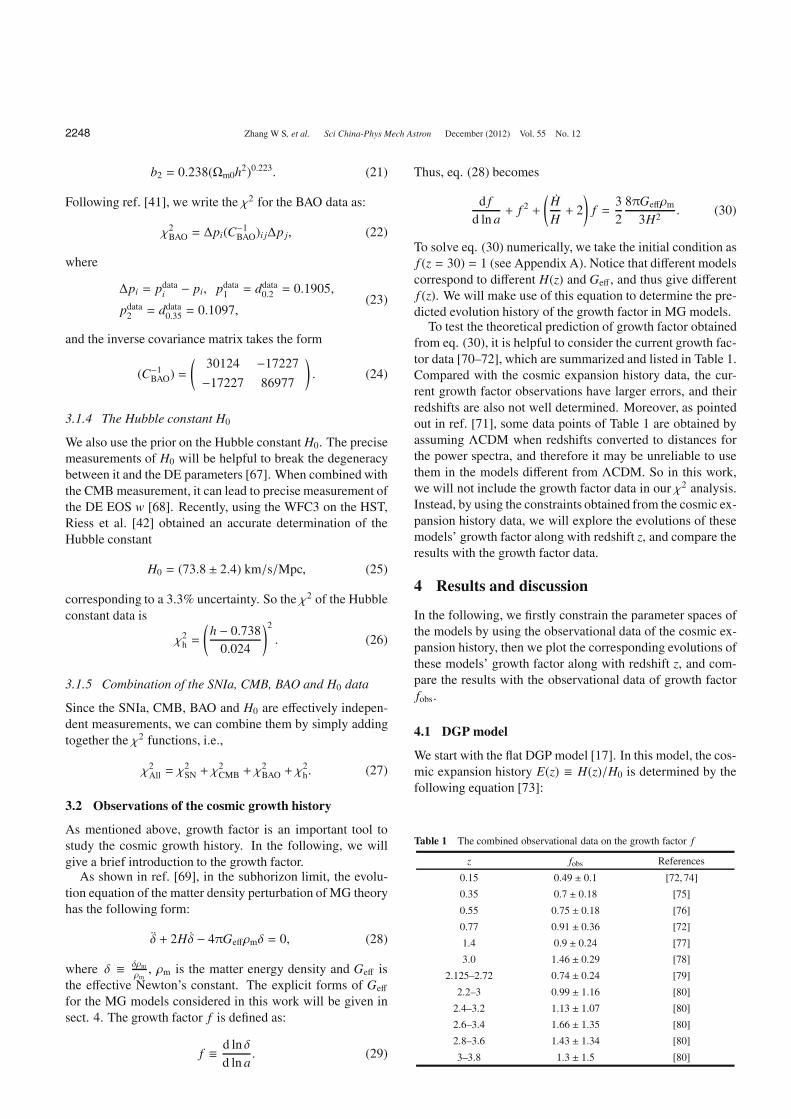
To test the theoretical prediction of growth factor obtainedfrom eq. (30), it is helpful to consider the current growth fac-tor data [70–72], which are summarized and listed in Table 1.Compared with the cosmic expansion history data, the cur-rent growth factor observations have larger errors, and theirredshifts are also not well determined. Moreover, as pointedout in ref. [71], some data points of Table 1 are obtained byassuming !CDM when redshifts converted to distances forthe power spectra, and therefore it may be unreliable to usethem in the models di"erent from !CDM. So in this work,we will not include the growth factor data in our !2 analysis.Instead, by using the constraints obtained from the cosmic ex-pansion history data, we will explore the evolutions of thesemodels’ growth factor along with redshift z, and compare theresults with the growth factor data.

4 Results and discussion

In the following, we firstly constrain the parameter spaces ofthe models by using the observational data of the cosmic ex-pansion history, then we plot the corresponding evolutions ofthese models’ growth factor along with redshift z, and com-pare the results with the observational data of growth factorfobs.

4.1 DGP model

We start with the flat DGP model [17]. In this model, the cos-mic expansion history E(z) # H(z)/H0 is determined by thefollowing equation [73]:

Table 1 The combined observational data on the growth factor f

z fobs References

0.15 0.49 ± 0.1 [72, 74]

0.35 0.7 ± 0.18 [75]

0.55 0.75 ± 0.18 [76]

0.77 0.91 ± 0.36 [72]

1.4 0.9 ± 0.24 [77]

3.0 1.46 ± 0.29 [78]

2.125–2.72 0.74 ± 0.24 [79]

2.2–3 0.99 ± 1.16 [80]

2.4–3.2 1.13 ± 1.07 [80]

2.6–3.4 1.66 ± 1.35 [80]

2.8–3.6 1.43 ± 1.34 [80]

3–3.8 1.3 ± 1.5 [80]

Zhang W S, et al. Sci China-Phys Mech Astron December (2012) Vol. 55 No. 12 2249

E(z) =- #%m0(1 + z)3 +%r0(1 + z)4 +%rc +

#%rc

.. (31)

Here, %rc = (1 " %m0 " %r0)2/4, and %r0 is the present frac-tional radiation density given by [40]

%r0 = %!0(1 + 0.2271Ne"), (32)

%!0 = 2.469 $ 10"5h"2, (33)

Ne" = 3.04, (34)

where %!0 is the present fractional photon density, and Ne"

is the e"ective number of neutrino species.In this model, the e"ective Newton constant Ge" is no

longer the simple constant G. Instead, it takes the followingform [81]:

Ge" = G2(1 + 2%2

m(z))

3(1 +%2m(z))

. (35)

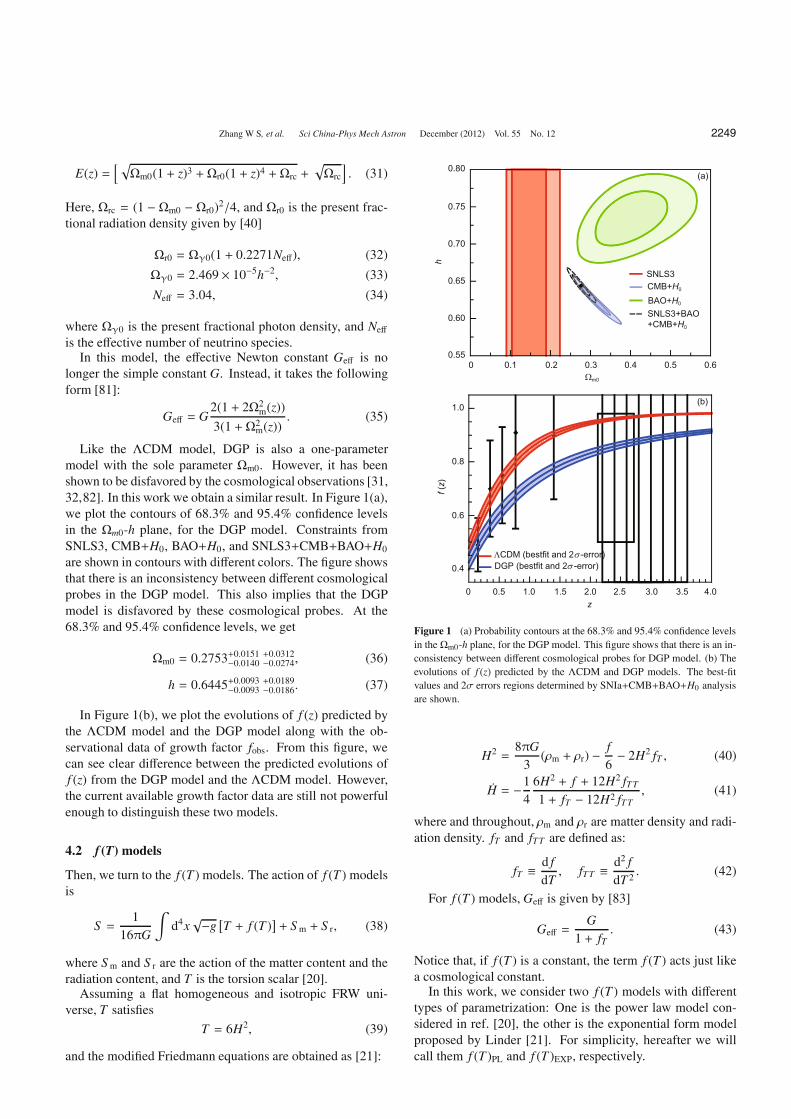
Like the !CDM model, DGP is also a one-parametermodel with the sole parameter %m0. However, it has beenshown to be disfavored by the cosmological observations [31,32,82]. In this work we obtain a similar result. In Figure 1(a),we plot the contours of 68.3% and 95.4% confidence levelsin the %m0-h plane, for the DGP model. Constraints fromSNLS3, CMB+H0, BAO+H0, and SNLS3+CMB+BAO+H0

are shown in contours with di"erent colors. The figure showsthat there is an inconsistency between di"erent cosmologicalprobes in the DGP model. This also implies that the DGPmodel is disfavored by these cosmological probes. At the68.3% and 95.4% confidence levels, we get

%m0 = 0.2753+0.0151"0.0140

+0.0312"0.0274, (36)

h = 0.6445+0.0093"0.0093

+0.0189"0.0186. (37)

In Figure 1(b), we plot the evolutions of f (z) predicted bythe !CDM model and the DGP model along with the ob-servational data of growth factor fobs. From this figure, wecan see clear di"erence between the predicted evolutions off (z) from the DGP model and the !CDM model. However,the current available growth factor data are still not powerfulenough to distinguish these two models.

4.2 f (T) models

Then, we turn to the f (T ) models. The action of f (T ) modelsis

S =1

16!G

"d4x'"g 1

T + f (T )2+ S m + S r, (38)

where S m and S r are the action of the matter content and theradiation content, and T is the torsion scalar [20].

Assuming a flat homogeneous and isotropic FRW uni-verse, T satisfies

T = 6H2, (39)

and the modified Friedmann equations are obtained as [21]:

(a)

(b)

0.80

SNLS3CMB+H0

BAO+H0

SNLS3+BAO+CMB+H0

!m0

hf (

z)

0.70

0.60

0.65

0.55

0.75

0 0.1 0.2 0.3 0.4 0.5 0.6

1.0

0.8

0.6

0.4

0 0.5 1.0 1.5z

2.0 2.5 3.0 3.5 4.0

"CDM (bestfit and 2 -error)#DGP (bestfit and 2 -error)#

Figure 1 (a) Probability contours at the 68.3% and 95.4% confidence levelsin the %m0-h plane, for the DGP model. This figure shows that there is an in-consistency between di"erent cosmological probes for DGP model. (b) Theevolutions of f (z) predicted by the !CDM and DGP models. The best-fitvalues and 2# errors regions determined by SNIa+CMB+BAO+H0 analysisare shown.

H2 =8!G

3('m + 'r) "

f6" 2H2 fT , (40)

H = "14

6H2 + f + 12H2 fTT

1 + fT " 12H2 fTT, (41)

where and throughout, 'm and 'r are matter density and radi-ation density. fT and fTT are defined as:

fT #d fdT, fTT #

d2 fdT 2 . (42)

For f (T ) models, Ge" is given by [83]

Ge" =G

1 + fT. (43)

Notice that, if f (T ) is a constant, the term f (T ) acts just likea cosmological constant.

In this work, we consider two f (T ) models with di"erenttypes of parametrization: One is the power law model con-sidered in ref. [20], the other is the exponential form modelproposed by Linder [21]. For simplicity, hereafter we willcall them f (T )PL and f (T )EXP, respectively.

2250 Zhang W S, et al. Sci China-Phys Mech Astron December (2012) Vol. 55 No. 12

4.2.1 The f (T )PL model

The power law model [20] assumes the following ansatz off (T ),

f (T ) = $("T )n. (44)

Here $ can be obtained by matching the present matter den-sity %m0 [20] :

$ = (6H20)

1"n 1 " %m0

2n " 1. (45)

Making use of these two equations, eq. (40) can be writtenas:

E(z)2 = %m0(1+z)3+%r0(1+z)4+(1"%m0"%r0)E(z)2n. (46)

Correspondingly, we also obtain Ge" :

Ge" = G1

1 + n(1"%m0)1"2n

3H0H

42(1"n). (47)

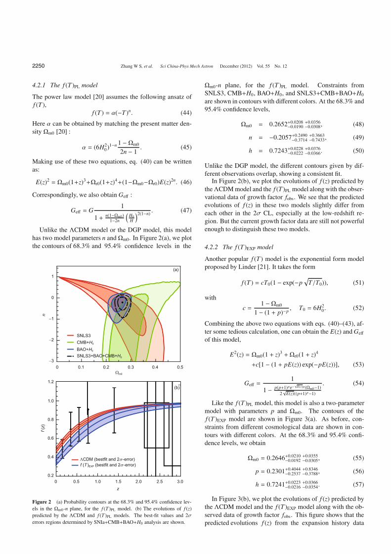
Unlike the !CDM model or the DGP model, this modelhas two model parameters n and %m0. In Figure 2(a), we plotthe contours of 68.3% and 95.4% confidence levels in the

SNLS3CMB+H0

BAO+H0

SNLS3+BAO+CMB+H0

"CDM (bestfit and 2 -error)#f (T )EXP (bestfit and 2 -error)#

!m0

0 0.1 0.2 0.3 0.4 0.5

0 0.5 1.0 1.5z

2.0 2.5 3.0

f (z)

1.0

1.2

0.8

0.6

0.4

0.2

1

0

$1

$2

$3

n

(a)

(b)

Figure 2 (a) Probability contours at the 68.3% and 95.4% confidence lev-els in the %m0-n plane, for the f (T )PL model. (b) The evolutions of f (z)predicted by the !CDM and f (T )PL models. The best-fit values and 2#errors regions determined by SNIa+CMB+BAO+H0 analysis are shown.

%m0-n plane, for the f (T )PL model. Constraints fromSNLS3, CMB+H0, BAO+H0, and SNLS3+CMB+BAO+H0

are shown in contours with di"erent colors. At the 68.3% and95.4% confidence levels,

%m0 = 0.2652+0.0208"0.0190

+0.0356"0.0308, (48)

n = "0.2057+0.2490"0.3714

+0.3663"0.7433, (49)

h = 0.7243+0.0228"0.0222

+0.0376"0.0366. (50)

Unlike the DGP model, the di"erent contours given by dif-ferent observations overlap, showing a consistent fit.

In Figure 2(b), we plot the evolutions of f (z) predicted bythe!CDM model and the f (T )PL model along with the obser-vational data of growth factor fobs. We see that the predictedevolutions of f (z) in these two models slightly di"er fromeach other in the 2# CL, especially at the low-redshift re-gion. But the current growth factor data are still not powerfulenough to distinguish these two models.

4.2.2 The f (T )EXP model

Another popular f (T ) model is the exponential form modelproposed by Linder [21]. It takes the form

f (T ) = cT0(1 " exp("p#

T/T0)), (51)

with

c =1 "%m0

1 " (1 + p)"p, T0 = 6H2

0 . (52)

Combining the above two equations with eqs. (40)–(43), af-ter some tedious calculation, one can obtain the E(z) and Ge"

of this model,

E2(z) = %m0(1 + z)3 +%r0(1 + z)4

+c[1 " (1 + pE(z)) exp("pE(z))], (53)

Ge" =1

1 " p(p+1)pe"'

E(z)p(%m0"1)2'

E(z)((p+1)p"1)

. (54)

Like the f (T )PL model, this model is also a two-parametermodel with parameters p and %m0. The contours of thef (T )EXP model are shown in Figure 3(a). As before, con-straints from di"erent cosmological data are shown in con-tours with di"erent colors. At the 68.3% and 95.4% confi-dence levels, we obtain

%m0 = 0.2646+0.0210"0.0192

+0.0355"0.0305, (55)

p = 0.2301+0.4044"0.2537

+0.8346"0.3788, (56)

h = 0.7241+0.0223"0.0216

+0.0366"0.0354. (57)

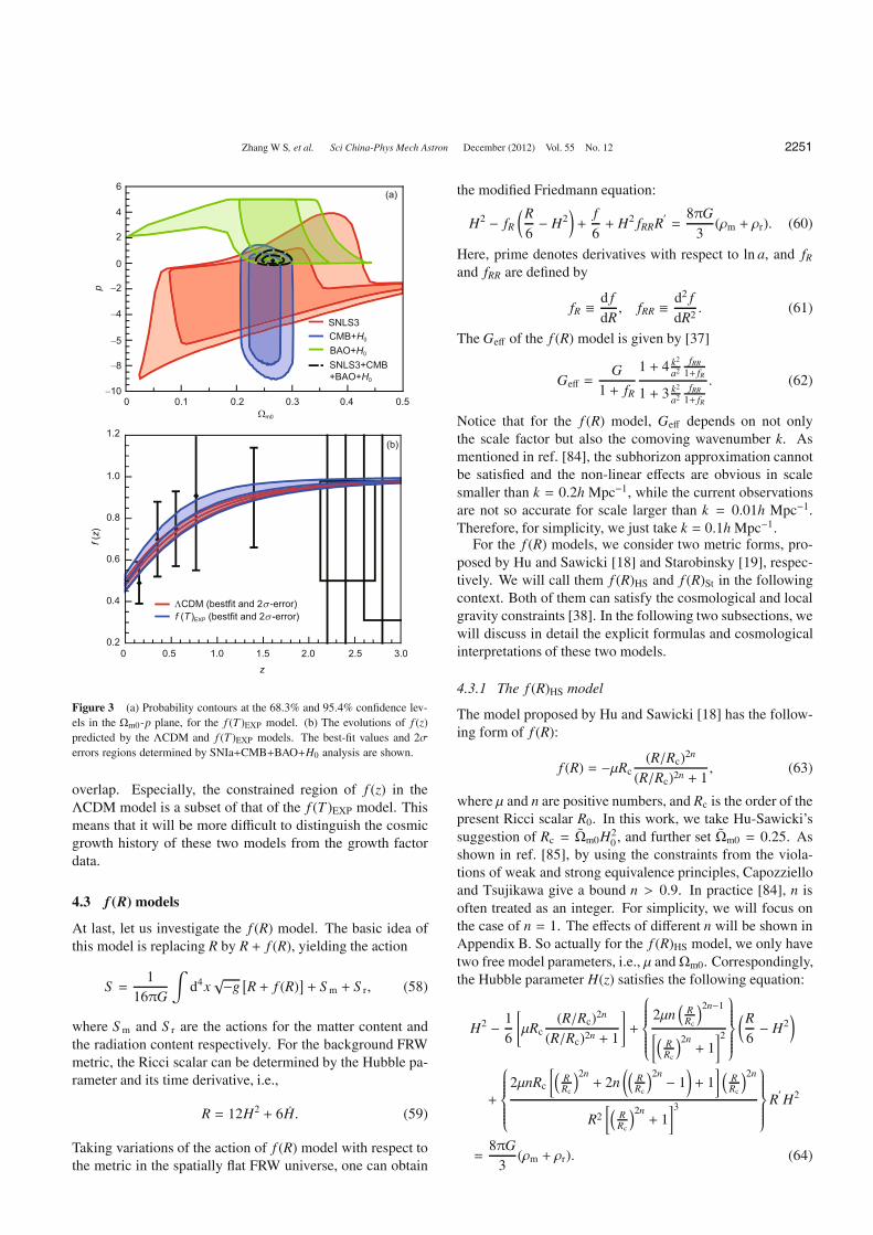
In Figure 3(b), we plot the evolutions of f (z) predicted bythe !CDM model and the f (T )EXP model along with the ob-served data of growth factor fobs. This figure shows that thepredicted evolutions f (z) from the expansion history data

Zhang W S, et al. Sci China-Phys Mech Astron December (2012) Vol. 55 No. 12 2251

f (z)

1.0

1.2

0.8

0.6

0.4

0.20 0.5 1.0 1.5

z2.0 2.5 3.0

!m0

0 0.1 0.2 0.3 0.4 0.5

6

0

2

4

$2

$5

$4

$10

$8

p

SNLS3CMB+H0

BAO+H0

SNLS3+CMB+BAO+H0

"CDM (bestfit and 2 -error)#f (T )EXP (bestfit and 2 -error)#

(a)

(b)

Figure 3 (a) Probability contours at the 68.3% and 95.4% confidence lev-els in the %m0-p plane, for the f (T )EXP model. (b) The evolutions of f (z)predicted by the !CDM and f (T )EXP models. The best-fit values and 2#errors regions determined by SNIa+CMB+BAO+H0 analysis are shown.

overlap. Especially, the constrained region of f (z) in the!CDM model is a subset of that of the f (T )EXP model. Thismeans that it will be more di$cult to distinguish the cosmicgrowth history of these two models from the growth factordata.

4.3 f (R) models

At last, let us investigate the f (R) model. The basic idea ofthis model is replacing R by R + f (R), yielding the action

S =1

16!G

"d4x'"g 1

R + f (R)2+ S m + S r, (58)

where S m and S r are the actions for the matter content andthe radiation content respectively. For the background FRWmetric, the Ricci scalar can be determined by the Hubble pa-rameter and its time derivative, i.e.,

R = 12H2 + 6H. (59)

Taking variations of the action of f (R) model with respect tothe metric in the spatially flat FRW universe, one can obtain

the modified Friedmann equation:

H2 " fR5R6" H2

6+

f6+ H2 fRRR

%=

8!G3

('m + 'r). (60)

Here, prime denotes derivatives with respect to ln a, and fRand fRR are defined by

fR #d fdR, fRR #

d2 fdR2 . (61)

The Ge" of the f (R) model is given by [37]

Ge" =G

1 + fR

1 + 4 k2

a2fRR

1+ fR

1 + 3 k2

a2fRR

1+ fR

. (62)

Notice that for the f (R) model, Ge" depends on not onlythe scale factor but also the comoving wavenumber k. Asmentioned in ref. [84], the subhorizon approximation cannotbe satisfied and the non-linear e"ects are obvious in scalesmaller than k = 0.2h Mpc"1, while the current observationsare not so accurate for scale larger than k = 0.01h Mpc"1.Therefore, for simplicity, we just take k = 0.1h Mpc"1.

For the f (R) models, we consider two metric forms, pro-posed by Hu and Sawicki [18] and Starobinsky [19], respec-tively. We will call them f (R)HS and f (R)St in the followingcontext. Both of them can satisfy the cosmological and localgravity constraints [38]. In the following two subsections, wewill discuss in detail the explicit formulas and cosmologicalinterpretations of these two models.

4.3.1 The f (R)HS model

The model proposed by Hu and Sawicki [18] has the follow-ing form of f (R):

f (R) = "µRc(R/Rc)2n

(R/Rc)2n + 1, (63)

where µ and n are positive numbers, and Rc is the order of thepresent Ricci scalar R0. In this work, we take Hu-Sawicki’ssuggestion of Rc = %m0H2

0 , and further set %m0 = 0.25. Asshown in ref. [85], by using the constraints from the viola-tions of weak and strong equivalence principles, Capozzielloand Tsujikawa give a bound n > 0.9. In practice [84], n isoften treated as an integer. For simplicity, we will focus onthe case of n = 1. The e"ects of di"erent n will be shown inAppendix B. So actually for the f (R)HS model, we only havetwo free model parameters, i.e., µ and%m0. Correspondingly,the Hubble parameter H(z) satisfies the following equation:

H2 " 16

+µRc

(R/Rc)2n

(R/Rc)2n + 1

,+

788888988888:

2µn3

RRc

42n"1

;3RRc

42n+ 1

<2

=88888>88888?

5R6" H2

6

+

788888988888:

2µnRc

;3RRc

42n+ 2n

53RRc

42n " 16+ 1

< 3RRc

42n

R2;3

RRc

42n+ 1

<3

=88888>88888?

R%H2

=8!G

3('m + 'r). (64)

2252 Zhang W S, et al. Sci China-Phys Mech Astron December (2012) Vol. 55 No. 12

One can solve this equation numerically to obtain the evolu-tion of H(z). From eqs. (62) and (63), the Ge" of this f (R)model can also be obtained.

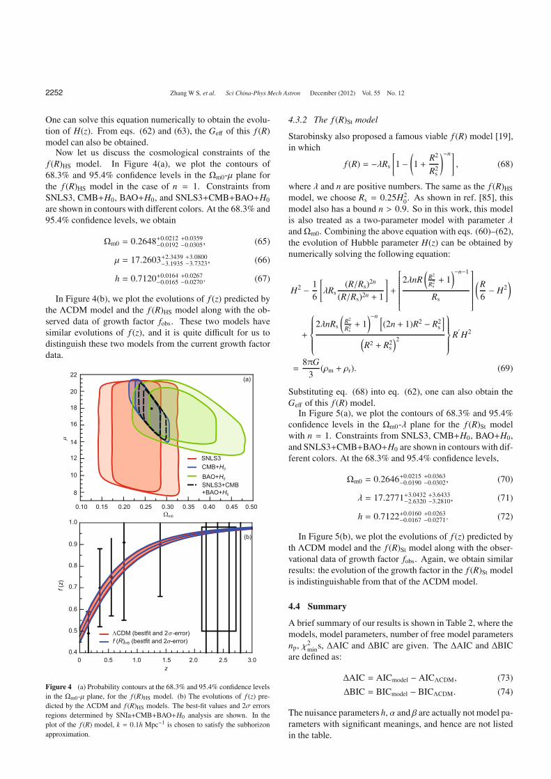
Now let us discuss the cosmological constraints of thef (R)HS model. In Figure 4(a), we plot the contours of68.3% and 95.4% confidence levels in the %m0-µ plane forthe f (R)HS model in the case of n = 1. Constraints fromSNLS3, CMB+H0, BAO+H0, and SNLS3+CMB+BAO+H0

are shown in contours with di"erent colors. At the 68.3% and95.4% confidence levels, we obtain

%m0 = 0.2648+0.0212"0.0192

+0.0359"0.0305, (65)

µ = 17.2603+2.3439"3.1935

+3.0800"3.7323, (66)

h = 0.7120+0.0164"0.0165

+0.0267"0.0270. (67)

In Figure 4(b), we plot the evolutions of f (z) predicted bythe !CDM model and the f (R)HS model along with the ob-served data of growth factor fobs. These two models havesimilar evolutions of f (z), and it is quite di$cult for us todistinguish these two models from the current growth factordata.

SNLS3CMB+H0

BAO+H0

SNLS3+CMB+BAO+H0

0 0.5 1.0 1.5z

2.0 2.5 3.0

f (z)

µ

(a)

(b)

"CDM (bestfit and 2 -error)#f (R)HS (bestfit and 2 -error)#

!m0

0.10 0.15 0.250.20 0.30 0.35 0.40 0.45 0.50

22

20

18

16

14

12

10

8

1.0

0.9

0.8

0.7

0.6

0.5

0.4

Figure 4 (a) Probability contours at the 68.3% and 95.4% confidence levelsin the %m0-µ plane, for the f (R)HS model. (b) The evolutions of f (z) pre-dicted by the !CDM and f (R)HS models. The best-fit values and 2# errorsregions determined by SNIa+CMB+BAO+H0 analysis are shown. In theplot of the f (R) model, k = 0.1h Mpc"1 is chosen to satisfy the subhorizonapproximation.

4.3.2 The f (R)St model

Starobinsky also proposed a famous viable f (R) model [19],in which

f (R) = "(Rs

+1 "

/1 +

R2

R2s

0"n,, (68)

where ( and n are positive numbers. The same as the f (R)HS

model, we choose Rs = 0.25H20. As shown in ref. [85], this

model also has a bound n > 0.9. So in this work, this modelis also treated as a two-parameter model with parameter (and%m0. Combining the above equation with eqs. (60)–(62),the evolution of Hubble parameter H(z) can be obtained bynumerically solving the following equation:

H2 " 16

+(Rs

(R/Rs)2n

(R/Rs)2n + 1

,+

@AAAAAAAAAAAAB

2(nR5

R2

R2s+ 1

6"n"1

Rs

CDDDDDDDDDDDDE

5R6" H2

6

+

788888988888:

2(nRs

5R2

R2s+ 1

6"n -(2n + 1)R2 " R2

s

.

3R2 + R2

s

42

=88888>88888?

R%H2

=8!G

3('m + 'r). (69)

Substituting eq. (68) into eq. (62), one can also obtain theGe" of this f (R) model.

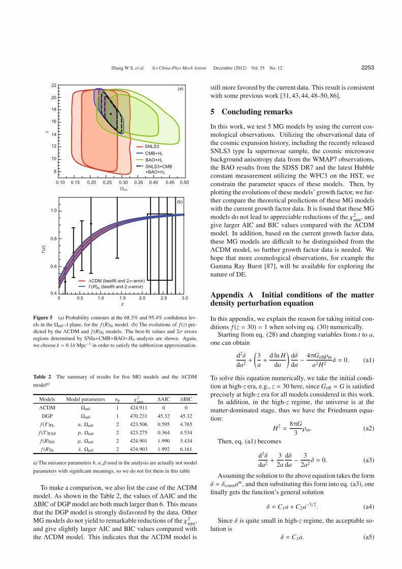
In Figure 5(a), we plot the contours of 68.3% and 95.4%confidence levels in the %m0-( plane for the f (R)St modelwith n = 1. Constraints from SNLS3, CMB+H0, BAO+H0,and SNLS3+CMB+BAO+H0 are shown in contours with dif-ferent colors. At the 68.3% and 95.4% confidence levels,

%m0 = 0.2646+0.0215"0.0190

+0.0363"0.0302, (70)

( = 17.2771+3.0432"2.6320

+3.6433"3.2810, (71)

h = 0.7122+0.0160"0.0167

+0.0263"0.0271. (72)

In Figure 5(b), we plot the evolutions of f (z) predicted byth !CDM model and the f (R)St model along with the obser-vational data of growth factor fobs. Again, we obtain similarresults: the evolution of the growth factor in the f (R)St modelis indistinguishable from that of the !CDM model.

4.4 Summary

A brief summary of our results is shown in Table 2, where themodels, model parameters, number of free model parametersnp, !2

mins, #AIC and #BIC are given. The #AIC and #BICare defined as:

#AIC = AICmodel " AIC!CDM, (73)

#BIC = BICmodel " BIC!CDM. (74)

The nuisance parameters h, $ and % are actually not model pa-rameters with significant meanings, and hence are not listedin the table.

Zhang W S, et al. Sci China-Phys Mech Astron December (2012) Vol. 55 No. 12 2253

f (z)

0.8

1.0

0.6

0.4

(a)

(b)

%

22

20

18

16

14

12

10

8

!m0

0.10 0.15 0.250.20 0.30 0.35 0.40 0.45 0.50

SNLS3CMB+H0

BAO+H0

SNLS3+CMB+BAO+H0

"CDM (bestfit and 2 -error)#f (R)St (bestfit and 2 -error)#

0 0.5 1.0 1.5z

2.0 2.5 3.0

Figure 5 (a) Probability contours at the 68.3% and 95.4% confidence lev-els in the %m0-( plane, for the f (R)St model. (b) The evolutions of f (z) pre-dicted by the !CDM and f (R)St models. The best-fit values and 2# errorsregions determined by SNIa+CMB+BAO+H0 analysis are shown. Again,we choose k = 0.1h Mpc"1 in order to satisfy the subhorizon approximation.

Table 2 The summary of results for five MG models and the !CDM

modela)

Models Model parameters np !2min #AIC #BIC

!CDM %m0 1 424.911 0 0

DGP %m0 1 470.231 45.32 45.32

f (T )PL n, %m0 2 423.506 0.595 4.765

f (T )EXP p, %m0 2 423.275 0.364 4.534

f (R)HS µ, %m0 2 424.901 1.990 5.434

f (R)St (, %m0 2 424.903 1.992 6.161

a) The nuisance parameters h, $, % used in the analysis are actually not model

parameters with significant meanings, so we do not list them in this table

To make a comparison, we also list the case of the !CDMmodel. As shown in the Table 2, the values of #AIC and the#BIC of DGP model are both much larger than 6. This meansthat the DGP model is strongly disfavored by the data. OtherMG models do not yield to remarkable reductions of the !2

min,and give slightly larger AIC and BIC values compared withthe !CDM model. This indicates that the !CDM model is

still more favored by the current data. This result is consistentwith some previous work [31, 43, 44, 48–50, 86].

5 Concluding remarks

In this work, we test 5 MG models by using the current cos-mological observations. Utilizing the observational data ofthe cosmic expansion history, including the recently releasedSNLS3 type Ia supernovae sample, the cosmic microwavebackground anisotropy data from the WMAP7 observations,the BAO results from the SDSS DR7 and the latest Hubbleconstant measurement utilizing the WFC3 on the HST, weconstrain the parameter spaces of these models. Then, byplotting the evolutions of these models’ growth factor, we fur-ther compare the theoretical predictions of these MG modelswith the current growth factor data. It is found that these MGmodels do not lead to appreciable reductions of the !2

min, andgive larger AIC and BIC values compared with the !CDMmodel. In addition, based on the current growth factor data,these MG models are di$cult to be distinguished from the!CDM model, so further growth factor data is needed. Wehope that more cosmological observations, for example theGamma Ray Burst [87], will be available for exploring thenature of DE.

Appendix A Initial conditions of the matterdensity perturbation equation

In this appendix, we explain the reason for taking initial con-ditions f (z = 30) = 1 when solving eq. (30) numerically.

Starting from eq. (28) and changing variables from t to a,one can obtain

d2&

da2+

/3a+

d ln Hda

0d&da" 4!Ge"'m

a2H2& = 0. (a1)

To solve this equation numerically, we take the initial condi-tion at high-z era, e.g., z = 30 here, since Ge" = G is satisfiedprecisely at high-z era for all models considered in this work.

In addition, in the high-z regime, the universe is at thematter-dominated stage, thus we have the Friedmann equa-tion:

H2 =8!G

3'm. (a2)

Then, eq. (a1) becomes

d2&

da2+

32a

d&da" 3

2a2& = 0. (a3)

Assuming the solution to the above equation takes the form& = &constam, and then substituting this form into eq. (a3), onefinally gets the function’s general solution

& = C1a + C2a"3/2. (a4)

Since & is quite small in high-z regime, the acceptable so-lution is

& = C1a. (a5)

2254 Zhang W S, et al. Sci China-Phys Mech Astron December (2012) Vol. 55 No. 12

Thus, we finally obtain the initial condition of eq. (30)

f =d ln &d ln a

= 1 (a6)

at redshift z = 30.

Appendix B The e!ects of n in the two f (R)models

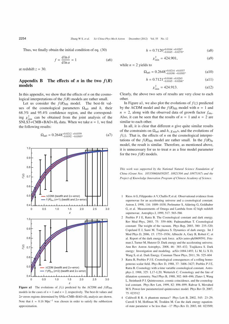
In this appendix, we show that the e"ects of n on the cosmo-logical interpretations of the f (R) models are rather small.

Let us consider the f (R)HS model. The best-fit val-ues of the cosmological parameters %m0 and h, their68.3% and 95.4% confidence region, and the correspond-ing !2

min can be obtained from the joint analysis of theSNLS3+CMB+BAO+H0 data. When we take n = 1, we findthe following results:

%m0 = 0.2648+0.0212"0.0192

+0.0359"0.0305, (a7)

0 0.5 1.0 1.5z

2.0 2.5 3.0

0 0.5 1.0 1.5z

2.0 2.5 3.0

f (z)

1.0

0.9

0.8

0.7

0.6

0.5

0.4

f (z)

1.0

0.9

0.8

0.7

0.6

0.5

0.4

"CDM (bestfit and 2 -error)#f (R)HS (n=1) (bestfit and 2 -error)#

"CDM (bestfit and 2 -error)#f (R)HS (n=2) (bestfit and 2 -error)#

Figure a1 The evolutions of f (z) predicted by the !CDM and f (R)HS

models in the cases of n = 1 and n = 2, respectively. The best-fit values and

2# errors regions determined by SNIa+CMB+BAO+H0 analysis are shown.

Note that k = 0.1h Mpc"1 was chosen in order to satisfy the subhorizon

approximation.

h = 0.7120+0.0164"0.0165

+0.0267"0.0270, (a8)

!2min = 424.901, (a9)

while n = 2 yields to

%m0 = 0.2648+0.0214"0.0190

+0.0357"0.0305, (a10)

h = 0.7121+0.0160"0.0165

+0.0265"0.0268, (a11)

!2min = 424.913. (a12)

Clearly, the above two sets of results are very close to eachother.

In Figure a1, we also plot the evolutions of f (z) predictedby the !CDM model and the f (R)HS model with n = 1 andn = 2, along with the observed data of growth factor fobs.Also, it can be seen that the results of n = 1 and n = 2 aresimilar to each other.

In all, it is clear that di"erent n give quite similar resultsof the constraints on %m0 and h, !mins, and the evolutions off (z). That is, the e"ects of n on the cosmological interpre-tations of the f (R)HS model are rather small. In the f (R)St

model, the result is similar. Therefore, as mentioned above,it is unnecessary for us to treat n as a free model parameterfor the two f (R) models.

This work was supported by the National Natural Science Foundation of

China (Grant Nos. 10535060/A050207, 10821504 and 10975167) and the

Project of Knowledge Innovation Program of Chinese Academy of Science.

1 Riess A G, Filippenko A V, Challis P, et al. Observational evidence fromsupernovae for an accelerating universe and a cosmological constant.Astron J, 1998, 116: 1009–1038; Perlmutter S, Aldering G, GoldhaberG, et al. Measurements of Omega and Lambda from 42 high redshiftsupernovae. Astrophys J, 1999, 517: 565–586

2 Peebles P J E, Ratra B. The Cosmological constant and dark energy.Rev Mod Phys, 2003, 75: 559–606; Padmanabhan T. Cosmologicalconstant: The weight of the vacuum. Phys Rep, 2003, 380: 235–320;Copeland E J, Sami M, Tsujikawa S. Dynamics of dark energy. Int JMod Phys D, 2006, 15: 1753–1936; Albrecht A, Gary B, Robert C, etal. Report of the dark energy task force. arXiv:astro-ph/0609591; Frie-man J, Turner M, Huterer D. Dark energy and the accelerating universe.Ann Rev Astron Astrophys, 2008, 46: 385–432; Tsujikawa S. Darkenergy: Investigation and modeling. arXiv:1004.1493; Li M, Li X D,Wang S, et al. Dark Energy. Commun Theor Phys, 2011, 56: 525–604

3 Ratra B, Peebles P J E. Cosmological consequences of a rolling homo-geneous scalar field. Phys Rev D, 1988, 37: 3406–3427; Peebles P J E,Ratra B. Cosmology with a time variable cosmological constant. Astro-phys J, 1988, 325: L17–L20; Wetterich C. Cosmology and the fate ofdilatation symmetry. Nucl Phys B, 1988, 302: 668–696; Zlatev I, WangL, Steinhardt P J. Quintessence, cosmic coincidence, and the cosmolog-ical constant. Phys Rev Lett, 1999, 82: 896–899; Rahvar S, MovahedM S. Power-law parameterized quintessence model. Phys Rev D, 2007,75: 023512

4 Caldwell R R. A phantom menace? Phys Lett B, 2002, 545: 23–29;Carroll S M, Ho"man M, Trodden M. Can the dark energy equation-of-state parameter w be less than "1? Phys Rev D, 2003, 68: 023509;

Zhang W S, et al. Sci China-Phys Mech Astron December (2012) Vol. 55 No. 12 2255

Huang T T, Wu P X, Yu H W. Observations favor the crossing of phan-tom divide lines. Sci China-Phys Mech Astron, 2010, 53(3): 562–566

5 Armendariz-Picon C, Damour T, Mukhanov V. k-inflation. Phys LettB, 1999, 458: 209–218; Armendariz-Picon C, Mukhanov V, SteinhardtP J. Essentials of k essence. Phys Rev D, 2011, 63: 103510; Chiba T,Okabe T, Yamaguchi M. Kinetically driven quintessence. Phys Rev D,2000, 62: 023511

6 Kamenshchik A Y, Moschella U, Pasquier V. An alternative toquintessence. Phys Lett B, 2001, 511: 265–268; Bento M C, BertolamiO, Sen A A. Generalized Chaplygin gas, accelerated expansion and darkenergy matter unification. Phys Rev D, 2002, 66: 043507; Zhang X, WuF Q, Zhang J. A New generalized Chaplygin gas as a scheme for unifi-cation of dark energy and dark matter. J Cosmol Astropart Phys, 2006,0601: 003; Li S, Ma Y G, Chen Y. Dynamical evolution of interactingmodified Chaplygin gas. Int J Mod Phys D, 2009, 18: 1785–1800

7 Padmanabhan T. Accelerated expansion of the universe driven by tachy-onic matter. Phys Rev D, 2002, 66: 021301; Bagla J S, Jassal H K, Pad-manabhan T. Accelerated expansion of the universe driven by tachyonicmatter. Phys Rev D, 2003, 67: 063504

8 Li M. A model of holographic dark energy. Phys Lett B, 2004, 603: 1–5;Huang Q G, Li M. The holographic dark energy in a non-flat universe.J Cosmol Astropart Phys, 2004, 0408: 013; Huang Q G, Gong Y G.Supernova constraints on a holographic dark energy model. J CosmolAstropart Phys, 2004, 0408: 006; Huang Q G, Li M. Anthropic princi-ple favors the holographic dark energy. J Cosmol Astropart Phys, 2005,0503: 001; Zhang X, Wu F Q. Constraints on holographic dark energyfrom Type Ia supernova observations. Phys Rev D, 2005, 72: 043524;Wang B, Abdalla E, Su R K. Constraints on the dark energy from holog-raphy. Phys Lett B, 2005, 611: 21–26; Wang B, Lin C Y, Abdalla E.Constraints on the interacting holographic dark energy model. PhysLett B, 2006, 637: 357–361; Zhang J, Zhang X, Liu H Y. Holographicdark energy in a cyclic universe. Eur Phys J C, 2007, 52: 693–699; FengC J. Holographic cosmological constant and dark energy. Phys Lett B,2008, 663: 367–371; Ma Y Z, Gong Y, Chen X L. Features of holo-graphic dark energy under the combined cosmological constraints. EurPhys J C, 2009, 60: 303–315; Li M, Li X D, Lin C S, et al. Holographicgas as dark energy. Commun Theor Phys, 2009, 51: 181–186; Li M,Li X D, Wang S, et al. Holographic dark energy models: A compari-son from the latest observational data. J Cosmol Astropart Phys, 2009,0906: 036; Li M, Li X D, Wang S, et al. Probing interaction and spatialcurvature in the holographic dark energy model. J Cosmol AstropartPhys, 2009, 0912: 014; Zhang X. Heal the world: Avoiding the cosmicdoomsday in the holographic dark energy model. Phys Lett B, 2010,683: 81–87; Wu Y B, Yang W Q, Wang C, et al. Modified Chaplygingas as an interacting holographic dark energy model. Sci China-PhysMech Astron, 2010, 53(4): 598–606

9 Wei H, Cai R G. Statefinder diagnostic and w " w% analysis for the age-graphic dark energy models without and with interaction. Phys Lett B,2007, 655: 1–6; Cai R G. A dark energy model characterized by theage of the universe. Phys Lett B, 2007, 657: 228–231; Wei H, Cai RG. A new model of agegraphic dark energy. Phys Lett B, 2008, 660:113–117; Wei H, Cai R G. Cosmological constraints on new agegraphicdark energy. Phys Lett B, 2008, 663: 1–6; Zhang J, Zhang X, Liu H.Agegraphic dark energy as a quintessence. Eur Phys J C, 2008, 54:303–309; Wu J P, Ma D Z, Ling Y. Quintessence reconstruction of thenew agegraphic dark energy model. Phys Lett B, 2008, 663: 152–159

10 Nojiri S, Odinitsov S D. Unifying phantom inflation with late-time ac-celeration: Scalar phantom-non-phantom transition model and general-ized holographic dark energy. Gen Rel Grav, 2006, 38: 1285–1304; GaoC, Wu F, Chen X, et al. A holographic dark energy model from Ricciscalar curvature. Phys Rev D, 2009, 79: 043511; Feng C J. Statefinder

diagnosis for Ricci dark energy. Phys Lett B, 2008, 670: 231–234; FengC J. Reconstructing quintom from Ricci dark energy. Phys Lett B, 2009,672: 94–97; Granda L N, Oliveros A. Infrared cut-o" proposal for theholographic density. Phys Lett B, 2008, 669: 275–277; Zhang X. Holo-graphic Ricci dark energy: Current observational constraints, quintomfeature, and the reconstruction of scalar-field dark energy. Phys RevD, 2009, 79: 103509; Feng C J, Zhang X. Holographic Ricci dark en-ergy in Randall-Sundrum braneworld: Avoidance of big rip and steadystate future. Phys Lett B, 2009, 680: 399–403; Li M, Li X D, Zhang X.Comparison of dark energy models: A perspective from the latest obser-vational data. Sci China-Phys Mech Astron, 2010, 53(9): 1631–1645;Wang T S, Liang N. Constraints on Cardassian universe from Gammaray bursts. Sci China-Phys Mech Astron, 2010, 53(9): 1720–1725

11 Wei H, Cai R G, Zeng D F. Hessence: A new view of quintom darkenergy. Class Quant Grav, 2005, 22: 3189–3202; Wei H, Cai R G. Cos-mological evolution of hessence dark energy and avoidance of big rip.Phys Rev D, 2005, 72: 123507

12 Zhang Y, Xia T Y, Zhao W. Yang-Mills condensate dark energy coupledwith matter and radiation. Class Quant Grav, 2007, 24: 3309–3338; XiaT Y, Zhang Y. 2-loop quantum Yang-Mills condensate as dark energy.Phys Lett B, 2007, 656: 19–24; Wang S, Zhang Y, Xia T Y. 3-loopYang-Mills condensate dark energy model. J Cosmol Astropart Phys,2008, 10: 037; Wang S, Zhang Y. Alleviation of cosmic age problem ininteracting dark energy model. Phys Lett B, 2008, 669: 201–205; ZhaiZ X, Liu W B. Constraints of f (R) gravity in Palatini approach withobservational Hubble data. Sci China-Phys Mech Astron, 2011, 54(8):1378–1383

13 Onemli V K, Woodard R P. Superacceleration from massless, minimallycoupled phi4. Class Quantum Grav, 2002, 19: 4607; Onemli V K,Woodard R P. Quantum e"ects can render w < "1 on cosmologicalscales. Phys Rev D, 2004, 70: 107301; Kahya E O, Onemli V K. Quan-tum stability of a w < "1 phase of cosmic acceleration. Phys Rev D,2007, 76: 043512

14 Weinberg S. The cosmological constant problem. Rev Mod Phys, 1989,61: 1–23; Carroll S M, Press W H, Turner E L. The cosmologicalconstant. Ann Rev Astron Astrophys, 1992, 30, 499–542; Sahni V,Starobinsky A. The case for a positive cosmological Lambda term. IntJ Mod Phys D, 2000, 9: 373–444; Carroll S M. The cosmological con-stant. Living Rev Rel, 2001, 4: 1–80

15 Nojiri S, Odinitsov S D. Unified cosmic history in modified gravity:From F(R) theory to Lorentz non-invariant models. Phys Rep, 2011,505: 59–144

16 Clifton T, Ferreira P G, Padilla A, et al. Modified gravity and cosmol-ogy. arXiv:1106.2476

17 Dvali G R, Gabadadze G, Porrati M. 4-D gravity on a brane in 5-DMinkowski space. Phys Lett B, 2000, 485: 208–214

18 Hu W, Sawicki I. Models of f (R) cosmic acceleration that evade solar-system tests. Phys Rev D, 2007, 76: 064004

19 Starobinsky A. Disappearing cosmological constant in f (R) gravity. JExp Theor Phys Lett, 2007, 86: 157–163

20 Bengochea G R, Ferraro R. Dark torsion as the cosmic speed-up. PhysRev D, 2009, 79: 124019

21 Linder E V. Einstein’s other gravity and the acceleration of the universe.Phys Rev D, 2010, 81: 127301

22 Yang R J. New types of f (T ) gravity. Eur Phys J C, 2010, 71: 1797;Yang R J. Conformal transformation in f (T ) theories. Europhys Lett,2011, 93: 60001

23 Milgrom M. A modification of the Newtonian dynamics as a possiblealternative to the hidden mass hypothesis. Astrophys J, 1983, 270: 365–370; Bekenstein J, Milgrom M. Does the missing mass problem signalthe breakdown of Newtonian gravity? Astrophys J, 1984, 286: 7–14;

2256 Zhang W S, et al. Sci China-Phys Mech Astron December (2012) Vol. 55 No. 12

Bekenstein J D. New gravitational theories as alternatives to dark mat-ter. In: Sato H, Nakamura T, eds. Proceedings of the Sixth MarcelGrossman Meeting on General Relativity. Singapore: World Scientific,1992

24 Bekenstein J D. Relativistic gravitation theory for the MOND paradigm.Phys Rev D, 2004, 70: 083509

25 Brans C, Dicke R H. Mach’s principle and a relativistic theory of grav-itation. Phys Rev, 1961, 124: 925–935; Amendola L. Scaling solu-tions in general nonminimal coupling theories. Phys Rev D, 1999, 60:043501

26 Zwiebach B. Curvature squared terms and string theories. Phys Lett B,1985, 156: 315–317

27 Horava P. Quantum gravity at a Lifshitz point. Phys Rev D, 2009, 79:084008; Saridakis E N. Horava-Lifshitz dark energy. Eur Phys J C,2010, 67: 229–235

28 Cahill R T, Rothall D. Discovery of uniformly expanding universe. ProgPhys, 2012, 1: 65–68; Cahill R T, Kerrigan D J. Dynamical space: Su-permassive galactic black holes and cosmic filaments. Prog Phys, 2011,4: 79–82

29 Nojiri S, Odintsov S D. Introduction to modified gravity and gravita-tional alternative for dark energy. Int J Geom Meth Mod Phys, 2007,4: 115–146; Sotiriou T P, Faraoni V. f (R) theories of gravity. Rev ModPhys, 2010, 82: 451–497; Felice A D, Tsujikawa S. f (R) theories. Liv-ing Rev Rel, 2010, 13: 3; Tsujikawa S. Modified gravity models of darkenergy. Lect Notes Phys, 2010, 800: 99–145

30 Sachs R K, Wolfe A M. Perturbations of a cosmological model and an-gular variations of the microwave background. Astrophys J, 1967, 147:73–90, reprinted Gen Rel Grav, 2007, 39: 1929–1961

31 Rubin D, Linder E V, Kowalski M, et al. Looking beyond Lambda withthe union supernova compilation. Astrophys J, 2009, 695: 391–403

32 Guo Z K, Zhu Z H, Alcaniz J S, et al. Constraints on the dgp modelfrom recent supernova observations and baryon acoustic oscillations.Astrophys J, 2006, 646: 1–7

33 Song Y S, Peiris H, Hu W. Cosmological constraints on f (R) acceler-ation models. Phys Rev D, 2007, 76: 063517; Zhao G B, TommasoG, Levon P, et al. Probing modifications of general relativity using cur-rent cosmological observations. Phys Rev D, 2010, 81: 103510; BambaK, Geng C Q, Lee C C. Cosmological evolution in exponential gravity.arXiv:1005.4574; Alal U, Varun S, Alexei A S. Reconstructing cosmo-logical matter perturbations using standard candles and rulers. Astro-phys J, 2009, 704: 1086–1097; Martinelli M, Melchiorri A, AmendolaL. Cosmological constraints on the Hu-Sawicki modified gravity sce-nario. Phys Rev D, 2009, 79: 123516; Wu P X, Yu H W. Observationalconstraints on f (T ) theory. Phys Lett B, 2010, 693: 415–420

34 Motohashi H, Starobinsky A, Yokoyama J. f (R) gravity and its cosmo-logical implications. Int J Mod Phys D, 2011, 20: 1347–1355; Ali A,Gannouji R, Sami M, et al. Background cosmological dynamics in f (R)gravity and observational constraints. Phys Rev D, 2010, 81: 104029;Carvalho F C, Santos E M, Alcaniz J S, et al. Cosmological constraintsfrom Hubble parameter on f (R) cosmologies. J Cosmol Astropart Phys,2008, 0809: 008; Dev A, Jain D, Jhingan S, et al. Delicate f (R) grav-ity models with disappearing cosmological constant and observationalconstraints on the model parameters. Phys Rev D, 2008, 78: 083515;Santos J, Alcaniz J S, Carvalho F C, et al. Latest supernovae constraintson f (R) cosmologies. Phys Lett B, 2008, 669: 14–18; Yang L, Lee C C,Luo L W, et al. Observational constraints on exponential gravity. PhysRev D, 2010, 82: 103515; Hirano K, Komiya Z. Observational con-straints on phantom crossing DGP gravity. Int J Mod Phys D, 2011, 20:1–16; Wan H Y, Yi Z L, Zhang T J. Constraints on the DGP universe us-ing observational Hubble parameter. Phys Lett B, 2007, 651: 352–356;Lue A, Scoccimarro R, Starkman G. Probing Newton’s constant on vast

scales: DGP gravity, cosmic acceleration and large scale structure. PhysRev D, 2004, 69: 124015; Acquaviva V, Hajian A, Spergel D N, et al.Next generation redshift surveys and the origin of cosmic acceleration.Phys Rev D, 2008, 78: 043514

35 Gong Y G. The growth factor parameterization and modified gravity.Phys Rev D, 2008, 78: 123010; Polarski D, Gannouji R. On the growthof linear perturbations. Phys Lett B, 2008, 660: 439–443; Linder E V.Cosmic growth history and expansion history. Phys Rev D, 2005, 72:043529; Koyama K, Maartens R. Structure formation in the dgp cos-mological model. J Cosmol Astropart Phys, 2006, 0601: 016; KoivistoT, Mota D F. Dark energy anisotropic stress and large scale structureformation. Phys Rev D, 2006, 73: 083502

36 Mota D F, Kristiansen J R, Koivisto T, et al. Constraining dark energyanisotropic stress. Mon Not R Astron Soc, 2007, 382: 793–800; DanielS, Caldwell R, Cooray A, et al. Large scale structure as a probe of grav-itational slip. Phys Rev D, 2008, 77: 103513; Knox L, Song Y S, TysonJ A. Distance-redshift and growth-redshift relations as two windows onacceleration and gravitation: Dark energy or new gravity? Phys Rev D,2006, 74: 023512; Ishak M, Upadhye A, Spergel D N. Probing cosmicacceleration beyond the equation of state: Distinguishing between darkenergy and modified gravity models. Phys Rev D, 2006, 74: 043513;Laszlo I, Bean R. Nonlinear growth in modified gravity theories of darkenergy. Phys Rev D, 2008, 77: 024048; Jain B, Zhang P. Observa-tional tests of modified gravity. Phys Rev D, 2008, 78: 063503; HuW, Sawicki I. A parameterized post-Friedmann framework for modifiedgravity. Phys Rev D, 2007, 76: 104043; Azizi T, Movahed M S, NozariK. Observational constraints on the normal branch of a warped DGPcosmology. New Astron, 2012, 17: 424–432; Baghram S, MovahedM S, Rahvar S. Observational tests of a two parameter power-law classmodified gravity in Palatini formalism. Phys Rev D, 2009, 80: 064003;

Movahed M S, Baghram S, Rahvar S. Consistency of f (R) =$

R2 " R20

gravity with the cosmological observations in Palatini formalism. PhysRev D, 2007, 76: 044008; Movahed M S, Farhang M, Rahvar S. Re-cent observational constraints on the DGP modified gravity. Int J TheorPhys, 2009, 48: 1203–1230

37 Tsujikawa S. Matter density perturbations and e"ective gravitationalconstant in modified gravity models of dark energy. Phys Rev D, 2007,76: 023514

38 Tsujikawa S. Observational signatures of f (R) dark energy models thatsatisfy cosmological and local gravity constraints. Phys Rev D, 2008,77: 023507

39 Conley A, Guy J, Sullivan M, et al. Supernova constraints and system-atic uncertainties from the first 3 years of the supernova legacy survey.Astrophys J Suppl Ser, 2011, 192: 1

40 Komatsu E, Smith K M, Dunkley J, et al. Seven-year Wilkinson Mi-crowave Anisotropy Probe (WMAP) observations: Cosmological inter-pretation. Astrophys J Suppl Ser, 2011, 192: 18

41 Percival W J, Reid B A, Eisenstein D J, et al. Baryon acoustic oscilla-tions in the sloan digital sky survey data release 7 galaxy sample. MonNot R Astron Soc, 2010, 401: 2148–2168

42 Riess A G, Macri L, Casertano S, et al. A 3% solution: Determinationof the Hubble constant with the Hubble space telescope and wide fieldcamera 3. Astrophys J, 2011, 730: 119

43 Akaike H. A new look at the statistical model identification. AutomControl IEEE Trans, 1974, 19: 716–723

44 Schwarz G. Estimating the dimension of a model. Ann Stat, 1978, 6:461–464

45 Starobinsky A. How to determine an e"ective potential for a variablecosmological term. J Exp Theor Phys Lett, 1998, 68: 757–763

46 Lewis A, Bridle S. Cosmological parameters from CMB and other data:A Monte Carlo approach. Phys Rev D, 2002, 66: 103511

Zhang W S, et al. Sci China-Phys Mech Astron December (2012) Vol. 55 No. 12 2257

47 Liddle A R. How many cosmological parameters? Mon Not R AstronSoc, 2004, 351: L49–L53

48 Godlowski W, Szydlowski M. Which cosmological model with dark en-ergy — phantom or lambda-CDM. Phys Lett B, 2005, 623: 10–16

49 Biesiada M. Information-theoretic model selection applied to super-novae data. J Cosmol Astropart Phys, 2007, 0702: 003

50 Magueijo J, Sorkin R D. Occam’s razor meets WMAP. Mon Not R As-tron Soc, 2007, 377: L39–L43

51 Liddle A R. Information criteria for astrophysical model selection. MonNot R Astron Soc Lett, 2007, 377: L74–L78

52 Guy J, Sullivan M, Conley A, et al. The supernova legacy survey 3-yearsample: Type Ia supernovae photometric distances and cosmologicalconstraints. arXiv:1010.4743

53 Hamuy M, Phillips M M, Suntze" N B, et al. BVRI light curves for29 Type Ia supernovae. Astron J, 1996, 112: 2408–2437; Riess A G,Kirshner R P, Schmidt B P, et al. BV RI light curves for 22 type Iasupernovae. Astron J, 1999, 117: 707–724; Jha S, Robert P K, PeterC, et al. Ubvri light curves of 44 type ia supernovae. Astron J, 2006,131: 527–554; Contreras C, Mario H, Phillips M M, et al. The carnegiesupernova project: First photometry data release of low-redshift type Iasupernovae. Astron J, 2010, 139: 519–539

54 Hicken M, Wood-Vasey W M, Blondin S, et al. Improved dark energyconstraints from (100 new CfA supernova type Ia light curves. Astro-phys J, 2009, 700: 1097–1140; Hicken M, Challis P, Jha S, et al. CfA3:185 type Ia supernova light curves from the CfA. Astrophys J, 2009,700: 331–357

55 Holtzman J A, Marriner J, Kessler R, et al. The sloan digital sky survey-II photometry and supernova IA light curves from the 2005 data. AstronJ, 2008, 136: 2306–2320

56 Riess A G, Louis-Gregory S, Stefano C, et al. New Hubble space tele-scope discoveries of type Ia supernovae at z >=1: Narrowing constraintson the early behavior of dark energy. Astrophys J, 2007, 659: 98–121

57 Sullivan M, Guy J, Conley A, et al. SNLS3: Constraints on dark en-ergy combining the supernova legacy survey three year data with otherprobes. Astrophys J, 2011, 737: 102

58 Li X D, Li S, Wang S, et al. Probing cosmic acceleration by using theSNLS3 SNIa dataset. J Cosmol Astropart Phys, 2011, 1107: 011

59 Wang Y, Chuang C H, Mukherjee P. A comparative study of dark energyconstraints from current observational data. arXiv:1109.3172

60 Gong Y G, Gao Q, Zhu Z H. The e"ect of di"erent observational dataon the constraints of cosmological parameters. arXiv:1110.6535

61 Li Z X, Wu P X, Yu H W. Testing nonstandard cosmologicalmodels with SNLS3 supernova data and other cosmological probes.arXiv:1109.6125

62 Sullivan M, Conley A, Howell D A, et al. The dependence of type Iasupernova luminosities on their host galaxies. Mon Not R Astron Soc,2010, 406: 782–802

63 Hu W, Sugiyama N. Small scale cosmological perturbations: An ana-lytic approach. Astrophys J, 1996, 471: 542–570

64 Bond J R, Efstathiou G, Tegmark M. Forecasting cosmic parameter er-rors from microwave background anisotropy experiments. Mon Not RAstron Soc, 1997, 291: L33–L41

65 Eisenstein D J, Zehavi I, Hogg D W, et al. Detection of the baryonacoustic peak in the large-scale correlation function of SDSS luminousred galaxies. Astrophys J, 2005, 633: 560–574

66 Eisenstein D J, Hu W. Baryonic features in the matter transfer function.Astrophys J, 1998, 496: 605

67 Freedman W J, Madore B F. The Hubble constant. arXiv:1004.1856

68 Hu W. Dark energy probes in light of the CMB. ASP Conf Ser, 2005,339: 215

69 Boisseau B, Esposito-Farse G, Polarski D, et al. Reconstruction of ascalar tensor theory of gravity in an accelerating universe. Phys RevLett, 2000, 85: 2236–2239

70 Porto C D, Amendola L. Observational constraints on the linear fluctu-ation growth rate. Phys Rev D, 2008, 77: 083508

71 Nesseris S, Perivolaropoulos L. Testing Lambda CDM with the growthfunction delta(a): Current constraints. Phys Rev D, 2008, 77: 023504

72 Guzzo L, Pierleoni M, Meneux B, et al. A test of the nature of cos-mic acceleration using galaxy redshift distortions. Nature, 2008, 451:541–545

73 De"ayet C. Cosmology on a brane in Minkowski bulk. Phys Lett B,2001, 502: 199–208; De"ayet C, Dvali G R, Gabadadze G. Accelerateduniverse from gravity leaking to extra dimensions. Phys Rev D, 2002,65: 044023

74 Colless M, Gavin D, Steve M, et al. The 2dF galaxy redshift survey:Spectra and redshifts. Mon Not R Astron Soc, 2001, 328: 1039–1063

75 Tegmark M, Eisenstein D J, Strauss M A, et al. Cosmological con-straints from the SDSS luminous red galaxies. Phys Rev D, 2006, 74:123507

76 Ross N P, da Angela J, Shanks T, et al. The 2dF-SDSS LRG and QSOsurvey: The 2-point correlation function and redshift-space distortions.Mon Not R Astron Soc, 2007, 381: 573–578

77 da Angela J, Shanks T, Croom S M. The 2dF-SDSS LRG and QSO sur-vey: QSO clustering and the L-z degeneracy. Mon Not R Astron Soc,2008, 383: 565–580

78 McDonald P, Seljak U, Cen R, et al. The linear theory power spectrumfrom the Lyman-alpha forest in the sloan digital sky survey. AstrophysJ, 2005, 635: 761–783

79 Viel M, Haehnelt M G, Springel V. Inferring the dark matter power spec-trum from the Lyman-alpha forest in high-resolution QSO absorptionspectra. Mon Not R Astron Soc, 2004, 354: 684–694

80 Viel M, Haehnelt M G, Springel V. Cosmological and astrophysical pa-rameters from the SDSS flux power spectrum and hydrodynamical sim-ulations of the Lyman-alpha forest. Mon Not R Astron Soc, 2006, 365:231–244

81 Lue A, Scoccimarro R, Starkman G. Di"erentiating between modifiedgravity and dark energy. Phys Rev D, 2004, 69: 044005

82 Fang W J, Wang S, Hu W, et al. Challenges to the DGP model fromHorizon-scale growth and geometry. Phys Rev D, 2008, 78: 103509;Fairbairn M, Goodbar A. Supernova limits on brane world cosmology.Phys Lett B, 2006, 642: 432–435; Maartens R, Majerotto E. Observa-tional constraints on self-accelerating cosmology. Phys Rev D, 2006,74: 023004; Alam U, Sahni V. Confronting braneworld cosmology withsupernova data and baryon oscillations. Phys Rev D, 2006, 73: 084024;Song Y S, Sawicki I, Hu W. Large-scale tests of the DGP model. PhysRev D, 2007, 75: 064003; Schmidt F. Self-consistent cosmological sim-ulations of DGP braneworld gravity. Phys Rev D, 2009, 80: 043001

83 Zheng R, Huang Q G. Growth factor in gravity. J Cosmol AstropartPhys, 2011, 1103: 002

84 Fu X Y, Wu P, Yu H. The growth factor of matter perturbations in f (R)gravity. Eur Phys J C, 2010, 68: 271–276

85 Capozziello S, Tsujikawa S. Solar system and equivalence principleconstraints on f (R) gravity by chameleon approach. Phys Rev D, 2008,77: 107501

86 Davis T M, Mortsell E, Sollerman J, et al. Scrutinizing exotic cosmo-logical models using ESSENCE supernova data combined with othercosmological probes. Astrophys J, 2007, 666: 716–725; SollermanJ, Mortsell E, Davis T M, et al. First-year sloan digital sky survey-II(SDSS-II) supernova results: Constraints on non-standard cosmologicalmodels. Astrophys J, 2009, 703: 1374–1385; Li M, Li X D, Zhang X.

2258 Zhang W S, et al. Sci China-Phys Mech Astron December (2012) Vol. 55 No. 12

Comparison of dark energy models: A perspective from the latest ob-servational data. Sci China-Phys Mech Astron, 2010, 53: 1631–1645;Wei H. Observational constraints on cosmological models with the up-dated long gamma-ray bursts. J Cosmol Astropart Phys, 2010, 1008:020

87 Schaefer B E. The Hubble diagram to redshift > 6 from 69 gamma-ray bursts. Astrophys J, 2007, 660: 16–46; Ghirlanda G, Ghisellini G,Firmani C. Gamma ray bursts as standard candles to constrain the cos-mological parameters. New J Phys, 2006, 8: 123; Liang E W. Gamma-ray bursts in the Swift-Fermi era: Confronting data with theory. SciChina-Phys Mech Astron, 2010, 53(Suppl. 1): 14–23; Xin L P, DengJ S, Zheng W K, et al. Three years’ systematic GRB follow-up at theXinglong Observatory and the optical afterglow observations of GRB080330. Sci China-Phys Mech Astron, 2010, 53(Suppl. 1): 56–59;Lin L, Liang E W, Zhang S N. GRB 090423: Marking the death of amassive star at z = 8.2. Sci China-Phys Mech Astron, 2010, 53(Suppl.1): 64–68; Deng J G, Liang E W. Correlation between pulse-width and

peak luminosity of single-pulse long gamma-ray bursts. Sci China-PhysMech Astron, 2010, 53(Suppl. 1): 69–72; Lv H J, Liang E W, Tong XF. Spectral properties of Fermi/GBM gamma-ray bursts and the GeVemission detection rate with Fermi/LAT. Sci China-Phys Mech Astron,2010, 53(Suppl. 1): 73–77; Dong W, Liang E W, Lu R J. The flux-E-p relation within GRB060218 in comparison with typical GRB pulses.Sci China-Phys Mech Astron, 2010, 53(Suppl. 1): 78–81; Lu Y, Gao H.A black hole preying on the star for a gamma-ray burst of GRB080503:Evidence for the second event in this new class. Sci China-Phys MechAstron, 2010, 53(Suppl. 1): 117–119; Wang X, Huang Y F, Kong S W.Constraint on the counter-jet emission in gamma-ray burst after-glowsfrom GRB 980703. Sci China-Phys Mech Astron, 2010, 53(Suppl. 1):259–261; Liu X W, Wu X F, Lu T. Magnetic energy injection in GRB080913. Sci China-Phys Mech Astron, 2010, 53(Suppl. 1): 262–264;Zheng W K, Deng J S. Evidence of a two-component jet in the after-glow of GRB 070419A. Sci China-Phys Mech Astron, 2010, 53(Suppl.1): 265–266