Testing Gravity with wide binary stars like Centauri · MNRAS 000,1{28(2018) Preprint 1 June 2018...
31
MNRAS 000, 1–31 (2018) Preprint 5 July 2018 Compiled using MNRAS L A T E X style file v3.0 Testing Gravity with wide binary stars like α Centauri Indranil Banik 1 * and Hongsheng Zhao 1 1 Scottish Universities Physics Alliance, University of St Andrews, North Haugh, St Andrews, Fife, KY16 9SS, UK 5 July 2018 ABSTRACT We consider the feasibility of testing Newtonian gravity at low accelerations using wide binary (WB) stars separated by & 3 kAU. These systems probe the accelerations at which galaxy rotation curves unexpectedly flatline, possibly due to Modified New- tonian Dynamics (MOND). We conduct Newtonian and MOND simulations of WBs covering a grid of model parameters in the system mass, semi-major axis, eccentricity and orbital plane. We self-consistently include the external field (EF) from the rest of the Galaxy on the Solar neighbourhood using an axisymmetric algorithm. For a given projected separation, WB relative velocities reach larger values in MOND. The excess is ≈ 20% adopting its simple interpolating function, as works best with a range of Galactic and extragalactic observations. This causes noticeable MOND effects in accurate observations of ≈ 500 WBs, even without radial velocity measurements. We show that the proposed Theia mission may be able to directly measure the orbital acceleration of Proxima Cen towards the 13 kAU-distant α Cen. This requires an astrometric accuracy of ≈ 1 μas over 5 years. We also consider the long-term orbital stability of WBs with different orbital planes. As each system rotates around the Galaxy, it experiences a time-varying EF because this is directed towards the Galactic Centre. We demonstrate approximate conservation of the angular momentum component along this direction, a consequence of the WB orbit adiabatically adjusting to the much slower Galactic orbit. WBs with very little angular momentum in this direction are less stable over Gyr periods. This novel direction-dependent effect might allow for further tests of MOND. Key words: gravitation – dark matter – proper motions – binaries: general – Galaxy: disc – stars: individual: Proxima Centauri 1 INTRODUCTION The currently prevailing cosmological paradigm (ΛCDM, Ostriker & Steinhardt 1995) is based on the assumption that General Relativity governs the dynamics of astrophys- ical systems. This can be well approximated by Newtonian gravity in the non-relativistic regime, covering for instance planetary motions in the Solar System and galactic rota- tion curves (Rowland 2015; de Almeida et al. 2016). While the former can be well described by Newtonian gravity, this is not the case for the latter (e.g. Rogstad & Shostak 1972). Moreover, self-gravitating Newtonian disks are un- stable both theoretically (Toomre 1964) and in numerical simulations (Hohl 1971). These apparently fatal problems with Newtonian grav- ity are generally explained by invoking massive halos of dark matter surrounding each galaxy (Ostriker & Peebles *Email: [email protected] (Indranil Banik) [email protected] (Hongsheng Zhao) 1973). Constraints from gravitational microlensing experi- ments indicate that the Galactic dark matter can’t be made of compact objects like stellar remnants (Alcock et al. 2000; Tisserand et al. 2007). Thus, it is hypothesised to be an undiscovered weakly interacting particle beyond the well- tested standard model of particle physics. While this may be the solution, it is conceivable that Newtonian gravity does in fact break down in some astro- physical systems (Zwicky 1937). If so, this would naturally explain the remarkably tight correlation between the in- ternal accelerations within galaxies (typically inferred from their rotation curves) and the prediction of Newtonian grav- ity applied to the distribution of their luminous matter (e.g. Famaey & McGaugh 2012, and references therein). This ‘ra- dial acceleration relation’ (RAR) has recently been tight- ened further based on near-infrared photometry taken by the Spitzer Space Telescope (Lelli et al. 2016), considering only the most reliable rotation curves (see their section 3.2.2) and taking advantage of reduced variability in stellar mass- to-light ratios at these wavelengths (Bell & de Jong 2001; c 2018 The Authors arXiv:1805.12273v3 [astro-ph.GA] 4 Jul 2018
Transcript of Testing Gravity with wide binary stars like Centauri · MNRAS 000,1{28(2018) Preprint 1 June 2018...
MNRAS 000, 1–31 (2018) Preprint 5 July 2018 Compiled using MNRAS LATEX style file v3.0
Testing Gravity with wide binary stars like α Centauri
Indranil Banik1∗ and Hongsheng Zhao11Scottish Universities Physics Alliance, University of St Andrews, North Haugh, St Andrews, Fife, KY16 9SS, UK
5 July 2018
ABSTRACT
We consider the feasibility of testing Newtonian gravity at low accelerations usingwide binary (WB) stars separated by & 3 kAU. These systems probe the accelerationsat which galaxy rotation curves unexpectedly flatline, possibly due to Modified New-tonian Dynamics (MOND). We conduct Newtonian and MOND simulations of WBscovering a grid of model parameters in the system mass, semi-major axis, eccentricityand orbital plane. We self-consistently include the external field (EF) from the restof the Galaxy on the Solar neighbourhood using an axisymmetric algorithm. For agiven projected separation, WB relative velocities reach larger values in MOND. Theexcess is ≈ 20% adopting its simple interpolating function, as works best with a rangeof Galactic and extragalactic observations. This causes noticeable MOND effects inaccurate observations of ≈ 500 WBs, even without radial velocity measurements.
We show that the proposed Theia mission may be able to directly measure theorbital acceleration of Proxima Cen towards the 13 kAU-distant α Cen. This requiresan astrometric accuracy of ≈ 1 µas over 5 years. We also consider the long-termorbital stability of WBs with different orbital planes. As each system rotates aroundthe Galaxy, it experiences a time-varying EF because this is directed towards theGalactic Centre. We demonstrate approximate conservation of the angular momentumcomponent along this direction, a consequence of the WB orbit adiabatically adjustingto the much slower Galactic orbit. WBs with very little angular momentum in thisdirection are less stable over Gyr periods. This novel direction-dependent effect mightallow for further tests of MOND.
Key words: gravitation – dark matter – proper motions – binaries: general – Galaxy:disc – stars: individual: Proxima Centauri
1 INTRODUCTION
The currently prevailing cosmological paradigm (ΛCDM,Ostriker & Steinhardt 1995) is based on the assumptionthat General Relativity governs the dynamics of astrophys-ical systems. This can be well approximated by Newtoniangravity in the non-relativistic regime, covering for instanceplanetary motions in the Solar System and galactic rota-tion curves (Rowland 2015; de Almeida et al. 2016). Whilethe former can be well described by Newtonian gravity,this is not the case for the latter (e.g. Rogstad & Shostak1972). Moreover, self-gravitating Newtonian disks are un-stable both theoretically (Toomre 1964) and in numericalsimulations (Hohl 1971).
These apparently fatal problems with Newtonian grav-ity are generally explained by invoking massive halos ofdark matter surrounding each galaxy (Ostriker & Peebles
∗Email: [email protected] (Indranil Banik)
[email protected] (Hongsheng Zhao)
1973). Constraints from gravitational microlensing experi-ments indicate that the Galactic dark matter can’t be madeof compact objects like stellar remnants (Alcock et al. 2000;Tisserand et al. 2007). Thus, it is hypothesised to be anundiscovered weakly interacting particle beyond the well-tested standard model of particle physics.
While this may be the solution, it is conceivable thatNewtonian gravity does in fact break down in some astro-physical systems (Zwicky 1937). If so, this would naturallyexplain the remarkably tight correlation between the in-ternal accelerations within galaxies (typically inferred fromtheir rotation curves) and the prediction of Newtonian grav-ity applied to the distribution of their luminous matter (e.g.Famaey & McGaugh 2012, and references therein). This ‘ra-dial acceleration relation’ (RAR) has recently been tight-ened further based on near-infrared photometry taken bythe Spitzer Space Telescope (Lelli et al. 2016), consideringonly the most reliable rotation curves (see their section 3.2.2)and taking advantage of reduced variability in stellar mass-to-light ratios at these wavelengths (Bell & de Jong 2001;
c© 2018 The Authors
arX
iv:1
805.
1227
3v3
[as
tro-
ph.G
A]
4 J
ul 2
018
2 Indranil Banik & Hongsheng Zhao
Norris et al. 2016). These improvements reveal that the RARholds with very little scatter over ≈ 5 orders of magnitudein luminosity and a similar range of surface brightness (Mc-Gaugh et al. 2016). Fits to individual rotation curves showthat any intrinsic scatter in the RAR must be < 13%.
In addition to disk galaxies, the RAR also holds forellipticals, whose internal accelerations can sometimes bemeasured accurately due to the presence of a thin rotation-supported gas disk (den Heijer et al. 2015). The RAR ex-tends down to galaxies as faint as the satellites of M31 (Mc-Gaugh & Milgrom 2013a). For a recent overview of how wellthe RAR works in several different types of galaxy across theHubble sequence, we refer the reader to Lelli et al. (2017).
Another long-standing issue faced by ΛCDM is thehighly anisotropic distribution of Milky Way (MW) satel-lites (Kroupa et al. 2005). Strongly flattened satellite sys-tems have also been identified around M31 (Ibata et al.2013) and Centaurus A (Muller et al. 2018). These struc-tures are difficult to reconcile with ΛCDM (Pawlowski 2018;Shao et al. 2018). Results from many different investigationsinto this issue are summarised in tables 1 and 2 of Forero-Romero & Arias (2018). Those authors use a different way ofquantifying asphericity but do not consider the particularlyproblematic velocity data. Even so, they find that the LGis a 3σ outlier to ΛCDM. Their section 4.4 also shows thatsimulations including baryonic effects have a more sphericalsatellite distribution, worsening the discrepancy.
The basic problem is that thin planar structures suggestsome dissipative mechanism. Although this is not by itselfunusual, dark matter is thought to be collisionless, with thelatest results arguing against the MW possessing a dark mat-ter disk (Schutz et al. 2017). Thus, the only natural way toform satellite planes is out of tidal debris expelled from thebaryonic disk of a galaxy that suffered an interaction withanother galaxy. This phenomenon occurs in some observedgalactic interactions (Mirabel et al. 1992). Due to the wayin which such tidal dwarf galaxies form out of a thin tidaltail, they would end up lying close to a plane and co-rotatingwithin that plane (Wetzstein et al. 2007).
Such a second-generation origin of the MW and M31satellite planes predicts that the satellites in these planesshould be free of dark matter (Barnes & Hernquist 1992;Wetzstein et al. 2007). This is due to the dissipation-less nature of dark matter and its initial distribution ina dispersion-supported near-spherical halo. During a tidalinteraction, dark matter of this form is clearly incapableof forming into a thin dense tidal tail out of which dwarfgalaxies might condense. Lacking dark matter, the MW andM31 satellite plane members should have very low internalvelocity dispersions σint .
This prediction is contradicted by the high observedσint of the MW satellites coherently rotating in a thinplane (McGaugh & Wolf 2010). The M31 satellite planegalaxies also have rather high σint (McGaugh & Milgrom2013b). This raises a serious objection to the idea that theanomalously strong internal accelerations within galaxies arecaused by their lying within massive dark matter halos.
The leading alternative explanation for these accel-eration discrepancies is Modified Newtonian Dynamics(MOND, Milgrom 1983). In MOND, the dynamical effectsusually attributed to dark matter are instead provided by anacceleration-dependent modification to gravity. The gravita-
tional field strength g at distance r from an isolated pointmass M transitions from the usual GM
r2law at short range
to
g =
√GMa0
rfor r �
rM︷ ︸︸ ︷√GM
a0
(1)
MOND introduces a0 as a fundamental accelerationscale of nature below which the deviation from Newtoniandynamics becomes significant. Empirically, a0 ≈ 1.2×10⁻¹⁰
m/s2 to match galaxy rotation curves (McGaugh 2011). Re-markably, this is similar to the acceleration at which theclassical energy density in a gravitational field (Peters 1981,equation 9) becomes comparable to the dark energy den-sity uΛ ≡ ρΛc
2 implied by the accelerating expansion of theUniverse (Riess et al. 1998). Thus,
g2
8πG< uΛ ⇔ g . 2πa0 (2)
This suggests that MOND may arise from quantumgravity effects (e.g. Milgrom 1999; Pazy 2013; Verlinde 2016;Smolin 2017). Regardless of its underlying microphysical ex-planation, it can accurately match the rotation curves of awide variety of both spiral and elliptical galaxies across avast range in mass, surface brightness and gas fraction (Lelliet al. 2017, and references therein). It is worth emphasisingthat MOND does all this based solely on the distribution ofluminous matter. Given that most of these rotation curveswere obtained in the decades after the MOND field equationwas first published (Bekenstein & Milgrom 1984), it is clearthat these achievements are successful a priori predictions.These predictions work due to underlying regularities ingalaxy rotation curves that are difficult to reconcile withthe collisionless dark matter halos of the ΛCDM paradigm(Salucci & Turini 2017; Desmond 2017a,b).
By generalising the Toomre disk stability condition(Toomre 1964) in Newtonian gravity, Milgrom (1989)showed that MOND is consistent with the stability of ob-served disk galaxies given reasonable velocity dispersions.This was later verified with numerical simulations, whichshowed that the change to the gravity law confers a similaramount of extra stability as a dark matter halo (Brada &Milgrom 1999). These simulations indicated a peculiarity ofMOND in low surface brightness galaxies (LSBs), whose lowaccelerations were predicted to be associated with a largeacceleration discrepancy. Though this was later verified (e.g.Famaey & McGaugh 2012), the discrepancy is convention-ally attributed to LSBs having a massive dark matter halothat dominates the enclosed mass down to very small radii.In MOND, all disk galaxies have self-gravitating disks, in-cluding LSBs. Thus, stability of a LSB in MOND requiresa higher minimum velocity dispersion compared to ΛCDM.Observed LSBs indeed have a rather high velocity dispersioncompared to the very low values feasible in ΛCDM for diskswhich are essentially not self-gravitating (Saburova 2011).
Of course, these LSBs could be dynamically overheatedas the Toomre condition only provides a lower limit to theirvelocity dispersion. This would make it difficult for LSBsto sustain spiral density waves, generally considered theexplanation for observed spiral features in higher surfacebrightness galaxies (Lin & Shu 1964). Interestingly, LSBs
MNRAS 000, 1–31 (2018)
Testing Gravity with wide binaries like α Centauri 3
also have spiral features (McGaugh et al. 1995). Assumingthe density wave theory applies there too, the number ofspiral arms gives an idea of the critical wavelength most un-stable to amplification by disk self-gravity. Indeed, D’Onghia(2015) was able to analytically predict rather accurately thenumber of spiral arms in galaxies observed as part of theDiskMass survey (Bershady et al. 2010), though this sur-vey ‘selects against LSB disks.’ Using this argument, Fuchs(2003) found that LSB disks need to be much more massivethan suggested by their photometry and stellar populationsynthesis models. A similar result was also reached by Peters& Kuzio de Naray (2018) using the pattern speeds of bars inLSBs, which are faster than expected in 3 of the 4 galaxiesthey considered.
Bars and spiral features in galaxies can be triggered byinteractions with satellites (Hu & Sijacki 2018). However,without disk self-gravity, any spirals formed in this waywould rapidly wind up and decay due to differential rotationof the disk (Fall & Lynden-Bell 1981, page 111). Even in agalaxy like M31, the simulations of Dubinski et al. (2008)indicate that interactions with a realistic satellite populationonly cause mild disk heating in excess of that which arisesin the absence of satellites.
Thus, evidence has been mounting over several decadesthat the gravity in a LSB generally comes from its disk. Thiscontradicts the ΛCDM expectation that it should mostlycome from its near-spherical halo of dark matter given thelarge acceleration discrepancy at all radii in LSBs. If this dis-crepancy arises due to MOND, then all galaxy disks wouldbe self-gravitating regardless of surface brightness.
Another consequence of the MOND scenario is that itraises the expected internal velocity dispersions of purelybaryonic MW and M31 satellites enough to match observa-tions (McGaugh & Wolf 2010; McGaugh & Milgrom 2013b,respectively). MOND also greatly enhances the mutual at-traction between the MW and M31. As a result, these galax-ies must have had a close flyby 9± 2 Gyr ago (Zhao et al.2013). We conducted simulations of this flyby, treating theMW and M31 as point masses surrounded by test particledisks. The outer particles of each disk generally ended uppreferentially rotating within a certain plane. If the flybyoccurred in a particular orientation, then both simulated‘satellite planes’ matched the orientations and spatial ex-tents of the corresponding observed structures (Banik et al.2018). Their best-fitting simulation also matched severalother constraints like the timing argument, the statementthat the MW and M31 must have been on the Hubble flowat very early times but still end up with their presentlyobserved separation and relative velocity (Kahn & Woltjer1959). The calculated flyby time of 7.65 Gyr ago correspondsfairly well to the observation that the vertical velocity dis-persion of the MW disk experienced a sudden jump ≈ 7Gyr ago (Yu & Liu 2018). The inner stellar halo of theMW accreted a significant proportion of its mass in a ‘majoraccretion event’ around that time (Belokurov et al. 2018).This strongly suggests that MOND can explain the LocalGroup satellite planes and perhaps also the Galactic thickdisk (Gilmore & Reid 1983) as a consequence of a past MW-M31 flyby. We are planning to test this scenario with N -body simulations similar to those conducted by Bılek et al.(2018).
As well as tidally affecting each other, the MW-M31
flyby would have dramatically affected the motion of LGdwarf galaxies caught near its spacetime location. The highMW-M31 relative velocity would allow them to gravitation-ally slingshot any nearby dwarf outwards at high speed,leading to some LG dwarfs having an unusually high radialvelocity for their position. We did in fact find some evidencefor 5 or 6 high-velocity galaxies (HVGs) like this (Banik &Zhao 2016, 2017), a result also confirmed by Peebles (2017)using his 3D ΛCDM model of the LG. We used a MONDmodel of the LG to demonstrate that the dwarfs reachingthe fastest speeds were likely flung out almost parallel tothe motion of the perturber. As a result, the HVGs oughtto define the MW-M31 orbital plane (Banik & Zhao 2018c,section 3). Observationally, the HVGs do define a rather thinplane, with the MW-M31 line only 16◦ out of this plane (seetheir table 4). Thus, we argued that the HVGs may preserveevidence of a past close MW-M31 flyby and their fast relativemotion at that time.
As well as enhancing the gravity between the MW andM31, MOND should also enhance the gravity exerted byother galaxy groups. This would cause them to have a largerturnaround radius at which a galaxy has zero radial velocitywith respect to the group. This turnaround radius is essen-tially a measure of where cosmic expansion wins the battleagainst the gravity of the cluster (Lee & Li 2017). Strongergravity would enlarge the turnaround radius, perhaps ex-plaining why it apparently exceeds the maximum expectedunder ΛCDM for the NGC 5353/4 group (Lee et al. 2015)and for three out of six other galaxy groups (Lee 2018).
Because MOND is an acceleration-dependent theory, itseffects could become apparent in a rather small system ifthe system had a sufficiently low mass (Equation 1). In fact,the MOND radius rM is only 7000 astronomical units (7kAU) for a system with M = M�. This implies that theorbits of distant Solar System objects might be affected byMOND (Pauco & Klacka 2016), perhaps accounting for cer-tain correlations in their properties (Pauco & Klacka 2017).For example, Oort cloud comets could fall into the innerSolar System more frequently as their orbits can lose theirangular momentum in MOND even without tidal effects(Section 9.2). However, it is difficult to accurately constrainthe dynamics of objects at such large distances.
Such constraints could be obtained more easily aroundother stars if they have distant binary companions. As firstsuggested by Hernandez et al. (2012), the orbital motions ofthese wide binaries (WBs) should be faster in MOND thanin Newtonian gravity. Moreover, it is likely that many suchsystems would form (Tokovinin 2017), paving the way forthe wide binary test (WBT) of gravity that we discuss inthis contribution.
The WBT was first attempted by Hernandez et al.(2012) using the WB catalogue of Shaya & Olling (2011),who applied Bayesian methods to Hipparcos data to iden-tify WBs within 100 pc (van Leeuwen 2007). A tentativesignal was identified whereby the typical relative velocitiesbetween WB stars remained constant with increasing sep-aration instead of following the expected Keplerian decline(Hernandez et al. 2012, figure 1). However, it was later shownthat their typical velocity uncertainty of 0.8 km/s was toolarge to allow meaningful conclusions about the underlyinglaw of gravity (Scarpa et al. 2017, section 1). Moreover, thelack of radial velocity measurements meant that a lot of the
MNRAS 000, 1–31 (2018)
4 Indranil Banik & Hongsheng Zhao
alleged systems were not in fact bound. Scarpa et al. (2017)attempted to overcome the latter problem using accuratespectra, thereby showing that a handful of systems werelikely genuine WBs that may be suitable for the WBT. Theyeven found a few systems whose relative velocity exceededthe Newtonian upper limit but fell below the MOND upperlimit, though additional follow-up work will be required toconfirm the nature of these systems.
Existing data from the Gaia mission (Perryman et al.2001) strongly suggests that many more WBs will be dis-covered (Andrews et al. 2017). The candidate systems theyidentified are mostly genuine, with a contamination rate of≈ 6% (Andrews et al. 2018) estimated using the second datarelease of the Gaia mission (Gaia DR2, Gaia Collaboration2018a).
The separations of WB stars are small compared totypical interstellar separations of ≈ 1 pc. As a result, anindividual WB system separated by 20 kAU should have acentre of mass acceleration towards the nearest star that is≈ 100× weaker than the internal gravity of the WB. Thetidal effect would be smaller still. Moreover, the effects ofstars in different directions would cancel to a large extent.For the Galaxy as a whole, the overall gravitational field isstill only∼ a0 despite the Solar neighbourhood lying∼ 105×further from the Galactic Centre than typical WB separa-tions. This implies that WBs should not be much affected bytides from the smooth component of the Galactic potential.
However, the real Galaxy is not smooth as it containsmany individual stars. Thus, one concern with the WBT iswhether a sufficiently large fraction of WB systems surviveencounters with passing field stars. Bahcall et al. (1985) esti-mated that the survival timescale was longer than 10 Gyr forsystems separated by < 31 kAU, with the survival timescaleand separation being inversely proportional to each other.Jiang & Tremaine (2010) also performed a detailed studyinto this issue. Their figure 8 shows that a substantial frac-tion of WB systems should survive for 10 Gyr if we restrict tosystems with separation below ≈ 0.1 of their Jacobi (tidal)radius, which is 350 kAU for two Sun-like stars orbiting eachother in the Solar neighbourhood (see their equation 43).
If WBs were very rare, then finding one should requireus to look beyond the nearest star to the Sun, Proxima Cen-tauri (Proxima Cen). It orbits the close (18 AU) binary αCen A and B at a distance of 13 kAU (Kervella et al. 2017).This puts the Proxima Cen orbit well within the regimewhere MOND would have a significant effect (Beech 2009,2011). Given the billions of stars in our Galaxy, it would behighly unusual if it did not contain a very large number ofsystems well suited to the WBT. This is especially true giventhe high (74%) likelihood that our nearest WB was stableover the last 5 Gyr despite the effects of Galactic tides andstellar encounters (Feng & Jones 2018).
Although these works assumed Newtonian gravity, theirconclusions should also be valid in MOND as the impulsedue to a stellar encounter would only be slightly enhancedin MOND (Figure 1). The effects of the non-linear MONDgravity can cause a WB to be unstable over Gyr periods,but we find that this only affects a small proportion of WBsystems in particular orientations (Section 9.2).
The WBT was considered in more detail by Pittordis& Sutherland (2018), who approximated MOND using theirequation 21. This appears to significantly underestimate the
gravitational attraction between the stars in a WB. In fact,the authors found a wide range of scenarios in which starsare expected to attract each other even less than underNewtonian gravity. Given the importance of the WBT, werevisit it using libraries of WB orbits based on more rig-orous MOND force calculations. These are compared withsimilar orbit libraries based on Newtonian gravity. We alsocheck our numerically determined MOND forces in very widesystems using previously derived analytic results (Banik &Zhao 2018a).
We then develop a statistical analysis procedure toquantify how many WB systems would be needed to conclu-sively distinguish between Newtonian and MOND gravityusing the WBT. Our work focuses on a particular imple-mentation of MOND with the interpolating function thatworks best with currently available observations. Thus, ourmore rigorous approach complements that of Pittordis &Sutherland (2018), who considered a wider range of modifiedgravity formulations and free parameters.
After introducing the WBT in Section 1, we explain howwe determine the MOND gravitational attraction betweenthe stars in each system and use this information to inte-grate the system (Section 2). We then discuss our choice ofprior distributions for the WB orbital parameters (Section3). Using similar methods to obtain a Newtonian control, wecompare the results using the procedure explained in Section4. This allows us to quantify how many systems are requiredfor the WBT, the primary result of this contribution (Sec-tion 5). We then discuss measurement uncertainties in thebasic parameters of nearby WB systems (Section 6). Usingsimple analytic estimates, we discuss how the WBT mightor might not work with different MOND formulations andinterpolating functions (Section 7). We also discuss whichinterpolating function is most appropriate in light of exist-ing observations, especially of rotation curves (Section 7.1).The WBT can also be affected by astrophysical uncertain-ties regarding the properties of each system, in particularwhether they contain any undetected companions (Section8). These uncertainties could be mitigated and a much moredirect version of the WBT conducted if the orbital accelera-tion were measured directly, something that may be possiblewith future observations of Proxima Cen (Section 9). In thissection, we also consider the long-term orbital stability ofWB systems in the complicated time-dependent MOND po-tential. We provide our conclusions in Section 10.
2 METHOD
The basic idea behind the WBT is that MOND enhancesthe gravitational attraction g between two widely separatedstars. Currently, it is difficult to test this by directly deter-mining their relative acceleration (though this may be possi-ble in future, see Section 9.1). Instead, the WBT focuses ontheir relative velocity v, making use of the fact that strongergravity allows systems to be bound at a higher relative speedv ≡ |v|.
One issue with the WBT is that it necessarily requiresmany WB systems and thus a sufficiently large survey vol-ume. Towards its edge, Gaia is unlikely to constrain lineof sight distances accurately enough to know the true (3D)
MNRAS 000, 1–31 (2018)
Testing Gravity with wide binaries like α Centauri 5
separation r of each system.1 However, the sky-projectedseparation rp would be known very accurately. To take ad-vantage of this, Pittordis & Sutherland (2018) defined
v ≡ v ÷
Newtonian vc︷ ︸︸ ︷√GM
rp(3)
v is the ratio of v to the Newtonian circular velocity vcof a system with total mass M if its stars are separated by adistance rp. Because their true (3D) separation r > rp, cal-
culating v in this way provides an upper limit on v÷√
GMr
,
a quantity which can’t exceed√
2 in Newtonian gravity. InMOND, we expect the upper limit to be somewhat higher.As a result, the probability distribution of v should differbetween the two models, with MOND allowing for a non-zero probability that v >
√2. This is the basis for the WBT.
To forecast how this might work, we integrate forwardsa grid of WB systems covering a range of masses and orbitalparameters. At each timestep, we consider what would beseen by a distant (� r) observer at a grid of possible viewingdirections. In this way, we build up a probability distributionover rp and v. The results are compared with those of simi-lar calculations using Newtonian gravity. We then develop astatistical procedure that quantifies how easily we could dis-tinguish the v distributions of the two theories for differenttotal numbers of WB systems (Section 4). This addressesthe question of how many systems would be needed for theWBT, thus helping observers plan its implementation.
In the near term, the WBT will be based on stars in theSolar neighbourhood. This means that our orbit integrationsmust take into account an important MOND phenomenonwhereby the internal dynamics of a system is affected byany external gravitational field gext, even if gext is uniformacross the system. This external field effect (EFE, Milgrom1986) arises because MOND gravity is non-linear in the mat-ter distribution (Section 4). The EFE can be understoodintuitively by considering a system with low internal accel-erations that would normally show strong MOND effects.However, if the system is in a high-acceleration environment(gext � a0), then the total acceleration g exceeds the a0
threshold, making the internal dynamics Newtonian.For the WBT, gext is provided by the rest of the Galaxy.
This leads to the force between two stars varying with theirorientation relative to the EF direction gext ≡ gext
|gext| . Thus,we need to consider WB systems with a range of differentangular momentum directions h. In general, all possible di-rections would need to be considered. To keep the computa-tional cost manageable, we make the simplifying assumptionthat one of the stars is much less massive than the other.This makes the problem axisymmetric as the gravitationalfield is generated by a single point mass, with the other startreated as a test particle.
Such a dominant mass approximation is valid in theNewtonian regime as the linearity of the gravity theorymeans the mass ratio has no effect on relative acceleration.Moreover, MOND gravity is also linear when gext dominatesthe dynamics of a system (Banik & Zhao 2018a). In thesecircumstances, the mass ratio between two stars does not
1 This information should be available for very nearby systems.
affect their relative acceleration (this depends only on theirtotal mass M and separation r).
Our approximation is therefore accurate both for veryclose and very wide systems. At intermediate separations,the force binding a WB system would be somewhat weakerif its mass were split more equally between its components(Milgrom 2010, equation 53). This would make the v distri-bution slightly more similar to the Newtonian expectation.However, we expect this to be a very small effect for reasonsdiscussed in Section 7.3.
2.1 Governing equations
We begin by describing how we advance WB systems usingthe quasilinear formulation of MOND (QUMOND, Milgrom2010). Each system is treated as a single point mass M plusa test particle embedded in a uniform EF gext. QUMONDuses the Newtonian gravitational field gN to determine thetrue gravitational field g by first finding its divergence.
∝ρPDM
+ρb︷ ︸︸ ︷
∇ · g = ∇ ·
νy︷ ︸︸ ︷(gNa0
)gN
where (4)
ν (y) =1
2+
√1
4+
1
y(5)
ν (y) is the interpolating function used to transitionbetween the Newtonian and deep-MOND regimes. We usethe ‘simple’ form of this function (Famaey & Binney 2005)because it fits a wide range of data on the MW and externalgalaxies better than other functions with a sharper tran-sition (Section 7.1). The source term for the gravitationalfield is ∇ · (νgN ), which can be thought of as an ‘effective’density ρ composed of the baryonic density ρb and an extracontribution which we define to be the phantom dark matterdensity ρPDM . This is the distribution of dark matter thatwould be necessary in Newtonian gravity to generate thesame total gravitational field as QUMOND yields from thebaryons alone.
The Newtonian gravity gN at position r relative to thecentral mass M is given by
gN ≡ − GMr
r3+ gN,ext (6)
The EF contributing to gN is not the true EF gextacting on the system. Rather, the important quantity isgN,ext , what the EF would have been if the universe wasgoverned by Newtonian gravity. For simplicity, we assumethe spherically symmetric relation between gext and gN,ext ,reducing Equation 4 to
νext gN,ext ≡ ν
(∣∣gN,ext
∣∣a0
)gN,ext = gext (7)
This algebraic MOND approximation should be fairlyaccurate given that the Solar neighbourhood is ≈ 4 diskscale lengths from the Galactic Centre (Bovy & Rix 2013;McMillan 2017). Note that this does not require the gravita-tional field to be spherically symmetric. Instead, it requiresthe weaker condition that departures of g from sphericalsymmetry are accurately captured by applying the MONDν function to gN , which is itself not spherically symmet-
MNRAS 000, 1–31 (2018)
6 Indranil Banik & Hongsheng Zhao
ric. This may explain why Jones-Smith et al. (2018) foundthat QUMOND gravitational fields in disk galaxies could beestimated rather well using the algebraic MOND approx-imation, justifying our use of Equation 7. We discuss itsaccuracy in Section 9.3.1, finding it should work well in theSolar neighbourhood where the WBT would be conducted.
Having found gN in this way, we use Equation 4 to find∇ · g. We then apply a direct summation procedure to thisin order to determine g itself.
g (r) =
∫∇ · g
(r′) (r − r′)
4π|r − r′|3 d3r′ (8)
As gN is axisymmetric about gext, the phantom darkmatter distribution can be thought of as a large number ofazimuthally uniform rings. At points along their symmetryaxis gext, it is thus straightforward to find g by summing thecontributions from each ring. In general, the lower mass starin a system is not conveniently located along gext relative tothe primary star. To find g at off-axis points in a computa-tionally efficient way, we use a ‘ring library’ that stores gN
due to a unit radius ring. This saves us from having to fur-ther split each ring into a finite number of elements. Instead,we can simply interpolate within our densely allocated ringlibrary to find the gravity exerted by any ring at the pointwhere we wish to know its contribution to g.
In this way, we can map out the gravitational field dueto a point mass M embedded in a uniform EF. Using ascaling trick, we only need to do this for one value of M .This is because the only physical lengths in the problem arethe MOND radius rM (Equation 1) and the EF radius rextwhere gN = gN,ext . If we keep gN,ext fixed, then it is alwaysa fixed multiple of a0 , leading to a constant rext
rM
. Thus, we
construct a force library for some arbitrary mass M = 1 andwork in units where G = a0 = 1, causing distances to be inunits of rM and accelerations in units of a0 .
Due to the finite extent of our grid, we can only con-sider contributions to g from the region r < rout , thoughwe make rout sufficiently large that gext is totally dominantbeyond it. Thus, regions beyond our grid have an analyticphantom density distribution containing only a quadrupolarterm (Banik & Zhao 2018a, equation 24). As explained inAppendix A, this leads to a correction ∆Φ to the potentialΦ in the region r < rout covered by our grid.
∆Φ (r, θ) =1
5GMνextK0r
2 (3 cos2 θ − 1) ∫ ∞
rout
1
r4dr
=GMνextK0r
2(3 cos2 θ − 1
)15rout
3where (9)
K0 ≡ ∂ Ln νext
∂ Ln gN,ext
= − 1
2if gN,ext � a0 (10)
cos θ = r · gext
This causes an adjustment to the gravitational field of
∆g =2GMνext
15 rout3(r − 3r cos θ gext) (11)
When considering a point where gext is dominant, the
gravity due to the star has a magnitude of ≈ GMνextr2
, mak-
ing the correction to it only ∼ 115
(r
rout
)3
when expressed in
fractional terms. Thus, the accuracy of our results should notdepend much on this correction, which should in any case be
very accurate as it estimates contributions from regions withr > 66.5 rM . There, g
N,extshould be should be & 5000 gN ,
allowing gN to be considered perturbatively in the mannerof Banik & Zhao (2018a).
In the opposite extreme where the test particle gets veryclose to the mass, we do not need to consider the EF due tothe rest of the Galaxy. Thus, at distances within 0.08 rM ,we assume that
g = νgN (12)
= − νGMr
r3(13)
At these positions, the EF (of order a0) should be& 100× weaker than gN , making it reasonable to treat thesituation as isolated and neglect the EF when calculating ν.However, our algorithm will eventually slow down if r be-comes sufficiently small. Thus, we terminate the trajectoryof any particle that gets within 50 AU.
2.2 The boost to Newtonian gravity
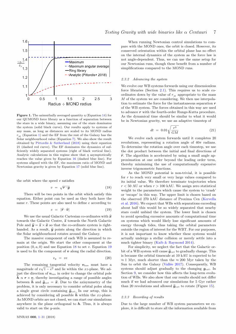
To better understand how much the gravity between twostars might be boosted by MOND effects, we determine theangle-averaged ratio η between the MOND and Newtonianradial gravity at different separations.
η (r) =1
4π
∫ π
0
gr (r, θ)
gN,r (r)2π sin θ dθ (14)
In very widely separated systems, the total accelerationis dominated by the EF rather than self-gravity g. In thislimit, we can obtain gr analytically (Banik & Zhao 2018a,equation 37).
gr = gN,r νext
(1 +
K0
2sin2 θ
)(15)
Substituting this into Equation 14 yields
η = νext
(1 +
K0
3
)(16)
The angle-averaging makes η a good guide to how muchgravity would be boosted by MOND effects in a system withknown separation relative to its MOND radius. In Figure 1,we compare the numerically determined value of η at differ-ent radii with this EF-dominated expectation.
For completeness, we note that the maximum value ofgrgN,r
requires not only that the EF dominate (gN,ext � g)
but also that the angle θ = 0 or π (Equation 15). Thus, theMOND boost to the self-gravity of the system is limited to
grgN,r
6 νext (17)
2.3 Orbit integration
2.3.1 Initial conditions
To investigate a range of WB orbital semi-major axes a andeccentricities e, we first need to define what these quantitiesmean in MOND. To generalise their definitions for modifiedgravity theories while remaining valid in Newtonian gravity,we follow the work of Pittordis & Sutherland (2018, section4.1). a is defined as the orbital separation r at the point in
MNRAS 000, 1–31 (2018)
Testing Gravity with wide binaries like α Centauri 7
Figure 1. The azimuthally averaged quantity η (Equation 14) for
our QUMOND force library as a function of separation betweenthe stars in a wide binary, assuming one of the stars dominates
the system (solid black curve). Our results apply to systems of
any mass, as long as distances are scaled to its MOND radiusrM (Equation 1) and the EF from the rest of the Galaxy has the
Solar neighbourhood value (Equation 7). We also show the result
obtained by Pittordis & Sutherland (2018) using their equation21 (dashed red curve). The EF dominates the dynamics of suf-
ficiently widely separated systems (right of black vertical line).Analytic calculations in this regime show that η asymptotically
reaches the value given by Equation 16 (dashed blue line). For
systems aligned with the EF, the maximum ratio of MOND andNewtonian gravity is given by Equation 17 (solid blue line).
the orbit where the speed v satisfies
v =√r · g (18)
There will be two points in the orbit which satisfy thisequation. Either point can be used as they both have thesame r. These points are also used to define e according to
e = |r · v| (19)
We use the usual Galactic Cartesian co-ordinates with xtowards the Galactic Centre, z towards the North GalacticPole and y = z × x so that the co-ordinate system is right-handed. As a result, y points along the direction in whichthe Solar neighbourhood rotates around the Galaxy.
The massive component of each WB is assumed to re-main at the origin. We start the other component at theposition (0, a, 0) and use Equation 18 to set v. Equation 19is used to fix the component of v along the radial direction.
vy = ve (20)
The remaining tangential velocity vtan must have amagnitude of v
√1− e2 and lie within the xz-plane. We ad-
just the direction of vtan in order to change the orbital poleh ∝ r × v, thereby investigating a range of possible anglesbetween h and gext = x. Due to the axisymmetry of theproblem, it is only necessary to consider orbital poles alonga single great circle containing gext. In our setup, this isachieved by considering all possible h within the xz-plane.As MOND orbits are not closed, we can start our simulationsanywhere in the plane orthogonal to h. Thus, it is alwaysvalid to start on the y-axis.
When running Newtonian control simulations to com-pare with the MOND ones, the orbit is closed. However, itsconserved orientation within the orbital plane has no effecton the internal dynamics of the system as the force law isnot angle-dependent. Thus, we can use the same setup forour Newtonian runs, though these benefit from a number ofsimplifications compared to the MOND runs.
2.3.2 Advancing the system
We evolve our WB systems forwards using our dimensionlessforce libraries (Section 2.1). This requires us to scale co-ordinates down by the value of rM appropriate to the massM of the system we are considering. We then use interpola-tion to estimate the force for the instantaneous separation rof the WB system. The forces obtained in this way are usedto advance r with the fourth-order Runge-Kutta procedure.As the dynamical time should be similar to what it wouldbe in Newtonian gravity, we use an adaptive timestep of
dt = 0.01
√r3
GM(21)
We evolve each system forwards until it completes 20revolutions, representing a rotation angle of 40π radians.To determine the rotation angle over each timestep, we usethe dot product between the initial and final directions ofr. The algorithm is accelerated by using a small angle ap-proximation at one order beyond the leading order term,thereby minimising the use of computationally expensiveinverse trigonometric functions.
As the MOND potential is non-trivial, it is possiblefor r to reach very small or very large values compared toits initial value. We therefore terminate trajectories whenr < 50 AU or when r > 100 kAU. We assign zero statisticalweight to the parameters which cause the system to ‘crash’or ‘escape’ in this way. The upper limit is chosen based onthe observed 270 kAU distance of Proxima Cen (Kervellaet al. 2016). We expect that WBs with separations exceedingabout half this would be so widely separated that nearbystars could unbind the system. The lower limit is chosento avoid spending excessive amounts of computational timeon systems which would likely lose significant amounts ofenergy through tides, thus taking the orbital parametersoutside the region of interest for the WBT. For our purposes,it is not important to know whether these systems wouldactually undergo a stellar collision or merely settle into amuch tighter binary (Kaib & Raymond 2014).
For simplicity, we neglect the fact that the Galactic or-bit of a WB system will cause gext to gradually change. Thisis because the orbital timescale at 10 kAU is expected to be≈ 1 Myr, much shorter than the ≈ 200 Myr taken by theSun to orbit the Galaxy (Vallee 2017). Consequently, WBsystems should adjust gradually to the changing gext. InSection 9, we consider how this affects the long-term evolu-tion of WBs. We also show that our results should not differmuch if we had advanced our simulations for 5 Gyr ratherthan 20 revolutions and allowed gext to rotate (Figure 15).
2.3.3 Recording of results
Due to the large number of WB system parameters we ex-plore, it is difficult to store all the information available from
MNRAS 000, 1–31 (2018)
8 Indranil Banik & Hongsheng Zhao
Variable Meaning Prior range
M Total system mass (1.2 − 2.4)M�
rp Sky-projected separation (1 − 20) kAUa Semi-major axis (1 − 60) kAU
eOrbital eccentricity (MOND) 0 − 0.95
e in Newtonian models 0 − 0.99γ See Equation 22 0, 1.2 (nominal), 2
γN γ for Newtonian model −2 to 2
Table 1. Our prior ranges on wide binary orbital parameters.Although we extract probabilities for sky-projected separations
rp up to 100 kAU, we assume that the WBT would be basedon systems with rp = (1 − 20) kAU to minimise contamination
by interlopers and avoid purely Newtonian systems. As the New-
tonian versions of these simulations are much faster, we use ahigher resolution and wider range in e. For each value of γ, we
try all possible values of γN and take the value which minimises
the detection probability (Section 4). Qualitatively, this yields aNewtonian v distribution most similar to the MOND one.
our trajectory calculations. Moreover, we are not interestedin doing so as the observations only constrain certain fea-tures of the orbits, and even then only in a statistical sensegiven that we see a very small fraction of the orbit. Thus, weuse our simulated trajectories to obtain the joint probabilitydistribution of the main observable quantities rp and v.
To do this, we create a 2D set of bins in rp and v. Ateach timestep and for each viewing angle (Section 3.5), weincrement the probability of the corresponding (rp, v) binby the duration of the timestep multiplied by the relativeprobability of that particular viewing angle. Afterwards, wenormalise the final probability distribution over (rp, v). If atrajectory crashes or escapes, then we assign zero probabilityto that particular combination of model parameters.
Our approach is valid as few WBs are destroyed on anorbital timescale (Section 8.1). As this is much shorter thana Hubble time, we assume the creation timescale of WBs isalso much longer than an individual orbit. This leads to the(rp, v) distribution remaining steady over many orbits.
3 PRIOR DISTRIBUTIONS OF BINARYPARAMETERS
For the WBT, we need prior distributions for the varioussystem parameters. The ones we consider are the semi-majoraxis a and eccentricity e (defined in Section 2.3.1), total
system mass M , the angle θ between h and gext and twoangles governing the direction from the WB system towardsthe observer. To allow easy investigation of different priorswithout rerunning the orbital integrations, we record theresulting P (rp, v) for the full grid of M , a and e. We donot store results for different angle parameters because weassume that they all have an isotropic distribution, allowingus to marginalise over them prior to recording the results(Sections 3.4 and 3.5).
3.1 Eccentricity
Following section 4.1 of Pittordis & Sutherland (2018), weassume the WB orbital eccentricity distribution P (e) has
the linear form
P (e) = 1 + γ
(e− 1
2
)(22)
The anti-symmetric factor(e− 1
2
)is required to ensure
the normalisation condition∫ 1
0P (e) de = 1. We assume
that the constant γ = 1.2 for the MOND case (Tokovinin &Kiyaeva 2016). To avoid negative probabilities, −2 6 γ 6 2.
When comparing with Newtonian gravity, it is necessaryto also define γN , the corresponding value of γ for the Newto-nian model. If the WBT yielded a positive result for MOND,then astronomers would almost certainly try to fit the datawith Newtonian gravity by adjusting γN . In general, tryingto match the high v values expected in MOND requiresNewtonian models with a large e as only such orbits canget v to significantly exceed 1. Giving a higher probabilityto high e orbits implies a higher γN .
As we do not a priori know γN , we need to let it varywhen estimating how easily the Newtonian and MOND vdistributions could be distinguished using the method de-scribed in Section 4. The ‘best-fitting’ γN is that whichmakes this task the most difficult. This requires us to con-sider all possible values for γN . Although γN can be negative,this would further reduce the probability of high e orbits,worsening the agreement with observations of a MOND uni-verse. Thus, we assume the optimal γN lies in the range(0, 2). Where it is clear that this is not the case becausenegative γN is preferred, we consider the full range of phys-ically possible values for γN (Section 5).
As the correct value of γ is not known either, we con-sider the three cases of 0 (a flat distribution), 1.2 (Tokovinin& Kiyaeva 2016) and 2. These were the three cases consid-ered by Pittordis & Sutherland (2018), as discussed in theirsection 2.1. Each time, we need to repeat our search for thebest-fitting γN .
3.2 Semi-major axis
To constrain the semi-major axis distribution P (a), we usethe observed P (rp) distribution (Andrews et al. 2017, sec-tion 6.2).1 Similar results were obtained by Lepine & Bon-giorno (2007), though with a slightly smaller break radius of4 kAU.
P (rp) drp ∝
{r−1p drp if rp 6 5 kAU
r−1.6p drp if rp > 5 kAU
(23)
To match these results, we use a broken power law forP (a) with the break at a = abreak .
P (a) da ∝{a−αda if a 6 abreak
a−βda if a > abreak
(24)
We consider a in the range (1− 60) kAU, though with alower resolution beyond 25 kAU. The lower limit of 1 kAU ischosen because the rather gradual interpolating function weadopt (Famaey & Binney 2005) implies that departures fromNewtonian gravity decay rather slowly as the accelerationrises above a0 . Moreover, tighter orbits are more common
1 Eventually, the distribution of 3D separations r will be usedfor this purpose, but GAIA is not expected to reach the requiredaccuracy (Section 6.2).
MNRAS 000, 1–31 (2018)
Testing Gravity with wide binaries like α Centauri 9
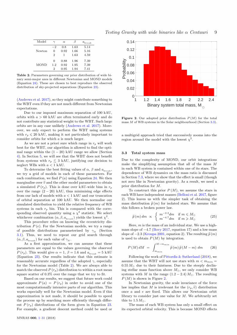
Model γ α β abreak
Newton
−2 0.8 1.63 5.14
0 0.92 1.66 5.16
2 1 1.63 4.59
MOND0 0.88 1.96 7.39
1.2 0.92 1.95 7.39
2 0.95 1.94 7.41
Table 2. Parameters governing our prior distribution of wide bi-
nary semi-major axes in different Newtonian and MOND models(Equation 24). These are chosen to best reproduce the observed
distribution of sky-projected separations (Equation 23).
(Andrews et al. 2017), so they might contribute something tothe WBT even if they are not much different from Newtonianexpectations.
Due to our imposed maximum separation of 100 kAU,orbits with a > 60 kAU are often terminated early and donot contribute any statistical weight to the WBT. Such largeorbits are in any case unlikely (Andrews et al. 2017). More-over, we only expect to perform the WBT using systemswith rp 6 20 kAU, making it not particularly important toconsider orbits for which a is much larger.
As we are not a priori sure which range in rp will workbest for the WBT, our algorithm is allowed to find the opti-mal range within the (1− 20) kAU range we allow (Section4). In Section 5, we will see that the WBT does not benefitfrom systems with rp . 3 kAU, justifying our decision toneglect WBs with a < 1 kAU.
To determine the best fitting values of α, β and abreak ,we try a grid of models in each of these parameters. Foreach combination, we find P (a) using Equation 24. We thenmarginalise over v and the other model parameters to obtaina simulated P (rp). This is done over kAU-wide bins in rpover the range (2− 20) kAU, thus minimising edge effectsfrom our lack of models with a < 1 kAU and our truncationof orbital separation at 100 kAU. We then normalise oursimulated distribution to yield the relative frequency of WBsystems in each rp bin. This is compared with the corre-sponding observed quantity using a χ2 statistic. We selectwhichever combination (α, β, abreak ) yields the lowest χ2.
This procedure relies on knowing the eccentricity dis-tribution P (e). For the Newtonian models, we try a rangeof possible distributions parameterised by γN (Section3.1). Thus, we need to repeat our grid search through(α, β, abreak ) for each value of γN .
As a first approximation, we can assume that theseparameters are equal to the values governing the observedP (rp). This would give α = 1, β = 1.6 and abreak = 5 kAU(Equation 23). Our results indicate that this estimate isreasonably accurate regardless of the adopted γ, especiallyfor the Newtonian model (Table 2). We are always able tomatch the observed P (rp) distribution to within a root meansquare scatter of 0.3% over the range that we try to fit.
Based on our results, we suggest that future work couldapproximate P (a) = P (rp) in order to avoid one of themost computationally intensive parts of our algorithm. Thisworks especially well for the Newtonian model. Even if thisapproximation is not made, it should be possible to speedthe process up by searching more efficiently through differ-ent P (rp) distributions of the form given in Equation 23.For example, a gradient descent method could be used or
1 1.2 1.4 1.6 1.8 2 2.2 2.4Binary system total mass, M
0
0.02
0.04
0.06
0.08
0.1
0.12
0.14
Pro
babi
lity
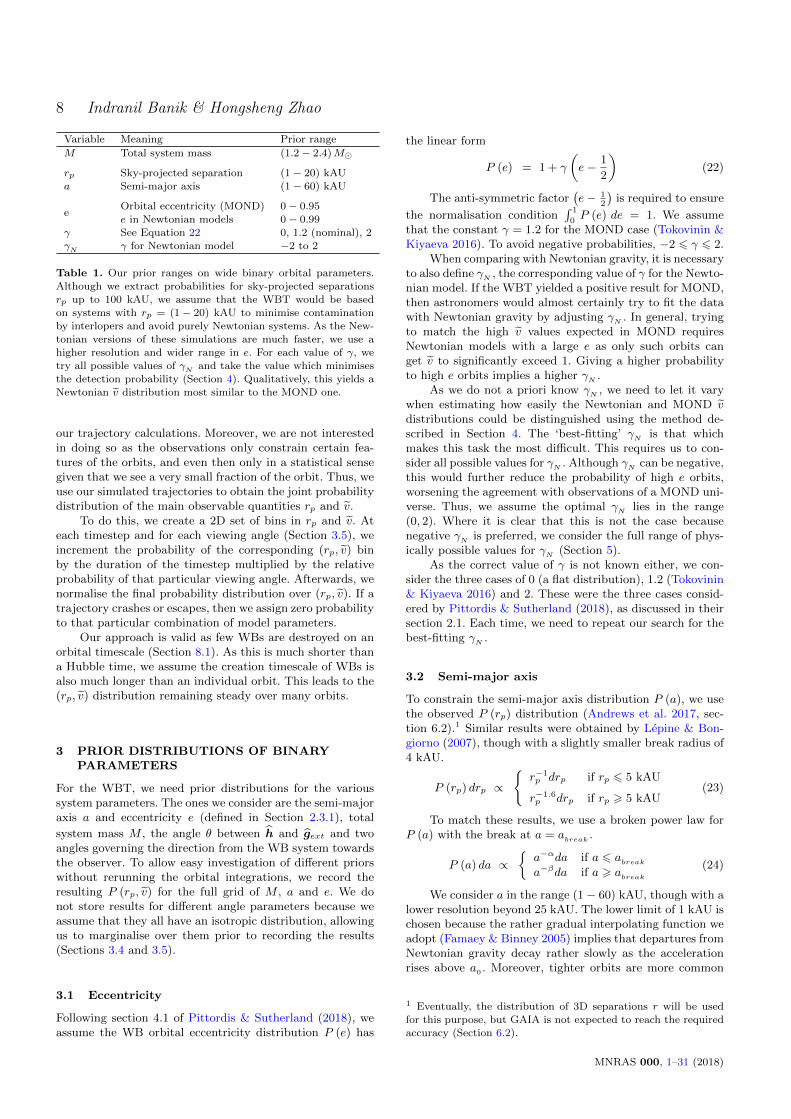
Figure 2. Our adopted prior distribution P (M) for the total
mass M of WB systems in the Solar neighbourhood (Section 3.3).
a multigrid approach tried that successively zooms into theregion around the model with the lowest χ2.
3.3 Total system mass
Due to the complexity of MOND, our orbit integrationsmake the simplifying assumption that all of the mass Min each WB system is contained within one of its stars. Thedependence of WB dynamics on the mass ratio is discussedin Section 7.3, where we show that the effect is small (thoughnot zero like in Newtonian gravity). As a result, we need aprior distribution for M .
To construct this prior P (M), we assume the stars ineach WB have independent masses (Belloni et al. 2017, figure2). This leaves us with the simpler task of obtaining themass distribution p (m) for isolated stars. We assume thatthis follows a broken power law.
p (m) dm ∝{m−2.3dm if m 6M�m−4.7dm if m >M�
(25)
Here, m is the mass of an individual star. We use a high-mass slope of −4.7 (Bovy 2017, equation 17) and a low-massslope of −2.3 (Kroupa 2001, equation 2). The resulting p (m)is used to obtain P (M) by integration.
P (M) dM =
∫ M−mmin
mmin
p (m) p (M −m) dm (26)
Following the work of Pittordis & Sutherland (2018), weassume that the WBT will not use stars with m < mmin =0.55M� due to their faintness. Due to the steeply declin-ing stellar mass function above M�, we only consider WBsystems with M in the range (1.2− 2.4)M�. The resultingP (M) is shown in Figure 2.
In Newtonian gravity, the scale invariance of the forcelaw implies that M is irrelevant for the (rp, v) distributiononce a and e are fixed. This allows our Newtonian orbitlibrary to consider just one value for M . We arbitrarily setthis to 1.5M�.
The mass of each WB system has only a small effect onits expected orbital velocity. This is because MOND effects
MNRAS 000, 1–31 (2018)
10 Indranil Banik & Hongsheng Zhao
arise at smaller separations in a lower mass system, coun-teracting the tendency of these systems to rotate slower.Using Equation 3 to estimate the circular velocity vc at theMOND radius rM (Equation 1) where MOND effects startto become significant, we see that
vc (rM ) ∝ 4√M (27)
Consequently, systems with total mass M = 1M� in-stead of 2M� would rotate only 16% slower, requiring asimilarly accurate velocity measurement. This suggests thatthe WBT could benefit from much better statistics if it usesobservations of lower mass systems. This would also allowcontamination to be reduced via a tighter cut on the pro-jected separation, as MOND effects would arise closer in(Equation 1).
In the short term, the most serious problem with thisis that lower mass stars are much less luminous (e.g. Mannet al. 2015). In the long run, this can be addressed with theuse of larger telescopes and longer exposures. Using morecommon systems also makes it more likely that there wouldbe a suitable background object within the same field of viewwhose true parallax and proper motion can be neglected,making it useful for calibration.
3.4 Orbital plane
Due to the presence of a preferred direction gext induced bythe EF, the behaviour of a WB system will depend some-what on the orientation of its orbital pole h with respect togext . As the WB orbital period is expected to be at mosta few Myr1, we do not expect gext to rotate significantlyduring a few WB orbits. Combined with our assumptionthat each WB system is dominated by one of the stars, thisleads to an axisymmetric potential. Consequently, the onlyphysically relevant aspect of h is its angle θ with gext .
We take this into account by considering a grid of pos-sible θ whose prior distribution P (θ) is assigned based on
the assumption that h is isotropically distributed.
P (θ) dθ =1
2sin θ dθ (28)
We only consider angles θ 6 π2
as larger angles areequivalent to a WB with a lower θ but with its initial velocityreversed. Because gravitational problems are time reversible,this should not affect WB characteristics like its averageorbital velocity. Such properties are thus expected to be thesame for θ → π − θ.
In the long term, the EF on each WB changes with timeas it rotates around the Galaxy. However, we do not expectthis to affect our results very much because the Galactic or-bit is much slower than the WB orbit. As a result, the initialdistribution of θ is likely preserved (Figure 17), maintaining
a nearly isotropic h distribution. This issue is discussed fur-ther in Section 9.2, where we show that the distribution inrp and v is nearly the same whether the orbit of ProximaCen is integrated for just 20 revolutions with a fixed EF orover 5 Gyr in a time-varying EF (Figure 15). This is becauseeach WB system is expected to have r go through a wide
1 using Kepler’s Third Law for stars similar to the Sun and aseparation below 20 kAU
range of directions relative to the EF such that the gravitybetween its stars follows an angular average. In any case,even an EF-dominated system in the Solar neighbourhoodshould not have a self-gravity that depends very much onits orientation relative to the EF (using K0 = −0.26 inEquation 15 shows that the force is affected at most 9%).
3.5 Viewing angle
Gaia observations are not expected to yield all six phasespace co-ordinates for most WB systems it discovers. Inparticular, the line of sight separation between the starswould generally not be known as accurately as the otherobservables (Pittordis & Sutherland 2018). The radial ve-locity difference between the stars may also be difficult todetermine at the∼ 0.1 km/s accuracy required for the WBT.In addition to accurate spectra, this also requires knowledgeof the difference in convective blueshift corrections betweenthe stars (Kervella et al. 2017). In the short run, this makes itinevitable that what we infer about each system will dependon its orientation relative to our line of sight towards it.
To take this into account, at each timestep of our WBorbital integrations, we consider a 2D grid of possible direc-tions n in which the observer lies relative to the WB system.Assuming the observer is much more distant than the WBseparation r, we determine rp using
rp = |r − (r · n) n| (29)
We use this in Equation 3 to find v, assuming massesare known regardless of the viewing angle as these shouldbe determined from luminosities of nearly isotropic stars(Section 6.3). We then increment the appropriate (rp, v) binby the fraction of the full 4π solid angle represented by eachn, assuming this has an isotropic distribution. This shouldbe valid out to the ≈ 150 pc distance relevant for the WBTas the MW disk scale height is larger (Ferguson et al. 2017,figure 7).
3.6 External field strength
We take the EF to point towards the Galactic centre andhave a magnitude sufficient to maintain the observed LocalStandard of Rest (LSR) speed of vc,� = 232.8 km/s, as-suming the Sun is R� = 8.2 kpc from the Galactic centre(McMillan 2017). Gaia DR2 remains consistent with theseparameters (Kawata et al. 2018).
We use Equation 7 to find the magnitude of theNewtonian-equivalent EF gN,ext from gext. Because gextfixed observationally, using a different MOND interpolationfunction alters gN,ext . We use the simple form of this func-tion for reasons discussed in Section 7.1.
In principle, Equation 7 is only valid in spherical sym-metry and is thus invalid near the MW disk and its resultingvertical force. However, this is expected to be rather smallin the Solar neighbourhood because we are ≈ 4 disk scalelengths from the Galactic Centre (Bovy & Rix 2013). Weconsider the accuracy of this algebraic MOND approxima-tion in Section 9.3.1. There, we show that the local value ofνext should be affected < 1% by the vertical gravity due tothe MW disk.
MNRAS 000, 1–31 (2018)
Testing Gravity with wide binaries like α Centauri 11
4 THE DETECTION PROBABILITY
Our primary objective is to obtain and compare the P (v)distributions for Newtonian and MOND gravity. We do thisby marginalising over WB parameters using the prior distri-butions outlined in Section 3. As our prior on a is alreadychosen to get an appropriate posterior distribution for rp(Section 3.2), marginalising over rp is simple. For consis-tency, we use the numerically determined P (rp) rather thanthe observed distribution, though the differences are verysmall (. 0.3% on average).
To compare the Newtonian PN (v) with the MONDPM (v), we use an algorithm that we make publicly avail-able.1 This provides a quantitative estimate of how easilywe can distinguish the two theories using N well-observedWB systems in different ranges of rp contained within theinterval (1− 20) kAU. In this way, we quantify how manysuch systems would be needed for the WBT. The actualnumber is likely to be somewhat larger due to observationaluncertainties (Section 6) and various systematic effects (Sec-tion 8). Moreover, not all WB systems will be suitable forthe WBT.
Our approach is to find the likelihood that observationsdrawn from PM (v) are inconsistent with expectations basedon PN (v). Suppose we have N = 100 systems and are inter-ested in the number n of them which have v > 1.2. If weexpect n = 9.7 in Newtonian gravity but a larger numberin MOND, then we begin by finding the maximum valueof n at the 99% confidence level according to PN (v). For-mally, this value nmax is the smallest integer which satisfiesP (n 6 nmax) > 0.99. Due to the discreteness of WB sys-tems, P (n) follows a binomial distribution whose parame-ters are (100, 0.097) in this example.
This leads to the conclusion that the Newtonian modelcould be used to explain any observed n 6 nmax = 16. Wethen find the likelihood that n > nmax if the observationscorrespond to a MOND universe. We call this likelihood thedetection probability Pdetection of MOND relative to Newto-nian gravity for the adopted prior distributions, (rp, v) rangeand number of systems used.
If we use a v range in which PM (v) has less probabilitythan PN (v), we reverse the logic outlined above. Thus, wefind the 99% confidence level lower limit of PN (v). We thendetermine the likelihood that n is even smaller if the observa-tions are drawn from PM (v). In practice, this situation doesnot arise because we expect the WBT to work best by focus-ing on high values of v which are more common in MOND.Even so, our analysis is not a blind search for discrepancieswith the Newtonian model but a more targeted search fordiscrepancies in the direction that would arise if MOND werecorrect. Blind analyses should also be conducted, especiallyif neither model describes the observations well.
When conducting our analysis, we try all possible rect-angular regions in (rp, v) space to see which one maximisesPdetection. We expect the algorithm to use the full range ofrp available to it (Table 1), but it is not clear a priori exactlywhich range of v will work best. This is because both modelspredict nearly 100% of systems within a very wide v range.If a very narrow range were used instead, it is quite possiblethat this has some probability of arising in MOND but no
1 Algorithm available at: MATLAB file exchange, code 65465
chance in Newtonian gravity. This is good for the WBT inthe sense that a detection within the adopted v range wouldconstitute very strong evidence for MOND. However, evenin MOND, it may be very unlikely to observe such a system.This would lead to a low Pdetection. Thus, some intermediaterange of v is expected to be most suitable for the WBT. Ourdiscussion so far suggests a range from the high end of theNewtonian v distribution to the upper limit of the MONDdistribution.
Although we are a priori unsure exactly which v rangeworks best, it is clear that the lower limit vmin of this rangeshould not be set above the maximum possible v in the New-tonian model. This is because raising vmin above this valuedoes not further reduce the already zero probability of find-ing a Newtonian WB system with v > vmin range. However,raising vmin does reduce the probability of finding a systemlike that if gravity were governed by MOND. Thus, raisingvmin above 1.42 can only ever reduce Pdetection. For this rea-son, we restrict the algorithm to only consider vmin 6 1.42.
The upper limit on v is not restricted apart from thebasic requirements to exceed vmin and to not exceed themaximum of 1.68 which arises in our MOND models. Intheory, selecting a larger value will not affect Pdetection. How-ever, in the real world, this would lead to additional sourcesof contamination that could hamper the WBT (Section 8).
If the data give any hint of a MOND signal, this willbe highly controversial and immediately raise many obser-vational and theoretical questions. On the theory side, as-tronomers would inevitably try a different γN , thus changingthe eccentricity distribution for the Newtonian model. Inparticular, higher values of γN would increase the weightgiven to highly eccentric orbits, making it more likely that vsignificantly exceeds 1. In future, it may be possible to pre-dict the Newtonian eccentricity distribution, thus reducingthis uncertainty. As this is not currently possible, we use themost conservative case where the value of γN is that whichmakes the WBT as difficult as possible. We find this bytrying a grid of possible values for γN , each time recordingPdetection. Whichever γN yields the lowest Pdetection thensets Pdetection for that particular value of N . In this way,we quantify how well the WBT can be expected to work fordifferent values of N and different model assumptions, bothfor Newtonian gravity and for MOND.
5 RESULTS
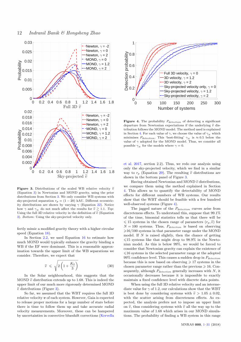
We begin by showing the v distributions P (v) for the Newto-nian and MOND models under various different assumptionsabout γ (Figure 3). The distributions are rather insensitiveto γ (Equation 22) in the region v & 1.1, a result also evidentfrom figure 2 of Pittordis & Sutherland (2018). Clearly, amuch larger fraction of WB systems have such a high v inMOND than in any plausible Newtonian model.
It may initially seem surprising that γN does not muchaffect the Newtonian v distribution for v & 1.1. After all,such high values of v are impossible for nearly circular orbitsbut quite possible for elliptical orbits. However, a highly el-liptical orbit spends the majority of its time near apocentre,where v is very low. Consequently, such an orbit will notcontribute much probability to the region v > 1.1. This iswhy Newtonian models with any value of γN can never per-
MNRAS 000, 1–31 (2018)
12 Indranil Banik & Hongsheng Zhao
0 0.2 0.4 0.6 0.8 1 1.2 1.4 1.6 1.80
0.005
0.01
0.015
0.02
0.025
0.03
Pro
babi
lity
Newton, = -2Newton, = 0Newton, = 2MOND, = 0MOND, = 1.2MOND, = 2
0 0.2 0.4 0.6 0.8 1 1.2 1.4 1.6 1.80
0.0020.0040.0060.008
0.010.0120.0140.0160.018
0.02
Pro
babi
lity
Newton, = -2Newton, = 0Newton, = 2MOND, = 0MOND, = 1.2MOND, = 2
Figure 3. Distributions of the scaled WB relative velocity v(Equation 3) in Newtonian and MOND gravity, using the prior
distributions from Section 3. We only consider WB systems withsky-projected separation rp = (1 − 20) kAU. Different eccentric-
ity distributions are shown by varying γ (Equation 22). Notice
how γ and γN do not much affect the results for v & 1.1. Top:Using the full 3D relative velocity in the definition of v (Equation
3). Bottom: Using the sky-projected velocity only.
fectly mimic a modified gravity theory with a higher circularspeed (Equation 18).
In Section 2.2, we used Equation 16 to estimate howmuch MOND would typically enhance the gravity binding aWB if the EF were dominant. This is a reasonable approx-imation towards the upper limit of the WB separations weconsider. Therefore, we expect that
v 6
√2
(1 +
K0
3
)(30)
In the Solar neighbourhood, this suggests that theMOND v distribution extends up to 1.68. This is indeed theupper limit of our much more rigorously determined MONDv distributions (Figure 3).
So far, we assumed that the WBT requires the full 3Drelative velocity v of each system. However, Gaia is expectedto release proper motions for a large number of stars beforethere is time to follow them up and take accurate radialvelocity measurements. Moreover, these can be hamperedby uncertainties in convective blueshift corrections (Kervella
0 50 100 150 200 250 300Number of systems
0
0.2
0.4
0.6
0.8
1
Det
ectio
n pr
obab
ility
Full 3D velocity, = 03D velocity, = 1.23D velocity, = 2Sky-projected velocity only, = 0Sky-projected velocity, = 1.2Sky-projected velocity, = 2
Figure 4. The probability Pdetection of detecting a significantdeparture from Newtonian expectations if the underlying v dis-
tribution follows the MOND model. The method used is explainedin Section 4. For each value of γ, we choose the value of γN which
minimises Pdetection. This ‘best-fitting’ γN is ≈ 0.5 below the
value of γ adopted for the MOND model. Thus, we consider allpossible γN for the models where γ = 0.
et al. 2017, section 2.2). Thus, we redo our analysis usingonly the sky-projected velocity, which we find in a similarway to rp (Equation 29). The resulting v distributions areshown in the bottom panel of Figure 3.
Having obtained Newtonian and MOND v distributions,we compare them using the method explained in Section4. This allows us to quantify the detectability of MONDeffects for different numbers of WB systems. Our resultsshow that the WBT should be feasible with a few hundredwell-observed systems (Figure 4).
The jagged nature of the Pdetection curves arise fromdiscreteness effects. To understand this, suppose that 99.1%of the time, binomial statistics tells us that there will be6 15 systems in the chosen range of parameters (rp, v) forN = 100 systems. Thus, Pdetection is based on observing>16/100 systems in that parameter range under the MONDmodel. If N is raised slightly, then the chance of getting615 systems like that might drop to 98.9% in the Newto-nian model. As this is below 99%, we would be forced toconsider that Newtonian gravity can explain the existence of616 systems in the selected parameter range at the adopted99% confidence level. This causes a sudden drop in Pdetectionbecause this is now based on observing > 17 systems in thechosen parameter range rather than the previous > 16. Con-sequently, although Pdetection generally increases with N , itoccasionally decreases because it is impossible to exactlymaintain a fixed confidence level with discrete data points.
When using the full 3D relative velocity and an interme-diate value for γ of 1.2, our calculations show that the WBTis best done by considering systems with v > 1.05 ± 0.02,with the scatter arising from discreteness effects. As ex-pected, the analysis prefers not to impose an upper limiton v, thus considering systems with v all the way up to themaximum value of 1.68 which arises in our MOND simula-tions. The probability of finding a WB system in this range
MNRAS 000, 1–31 (2018)
Testing Gravity with wide binaries like α Centauri 13
0 50 100 150 200 250 300Number of systems
0
0.2
0.4
0.6
0.8
1
Det
ectio
n pr
obab
ility
Full 3D velocity, rp 40 kAU
Full 3D velocity, rp 20 kAU
Full 3D velocity, rp 10 kAU
Velocity on sky, rp 40 kAU
Velocity on sky, rp 20 kAU
Velocity on sky, rp 10 kAU
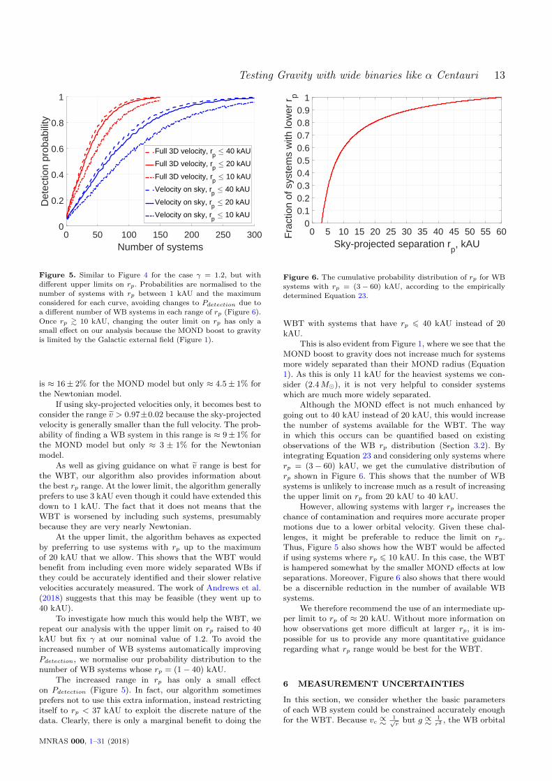
Figure 5. Similar to Figure 4 for the case γ = 1.2, but with
different upper limits on rp. Probabilities are normalised to thenumber of systems with rp between 1 kAU and the maximum
considered for each curve, avoiding changes to Pdetection due to
a different number of WB systems in each range of rp (Figure 6).Once rp & 10 kAU, changing the outer limit on rp has only a
small effect on our analysis because the MOND boost to gravity
is limited by the Galactic external field (Figure 1).
is ≈ 16± 2% for the MOND model but only ≈ 4.5± 1% forthe Newtonian model.
If using sky-projected velocities only, it becomes best toconsider the range v > 0.97±0.02 because the sky-projectedvelocity is generally smaller than the full velocity. The prob-ability of finding a WB system in this range is ≈ 9± 1% forthe MOND model but only ≈ 3 ± 1% for the Newtonianmodel.
As well as giving guidance on what v range is best forthe WBT, our algorithm also provides information aboutthe best rp range. At the lower limit, the algorithm generallyprefers to use 3 kAU even though it could have extended thisdown to 1 kAU. The fact that it does not means that theWBT is worsened by including such systems, presumablybecause they are very nearly Newtonian.
At the upper limit, the algorithm behaves as expectedby preferring to use systems with rp up to the maximumof 20 kAU that we allow. This shows that the WBT wouldbenefit from including even more widely separated WBs ifthey could be accurately identified and their slower relativevelocities accurately measured. The work of Andrews et al.(2018) suggests that this may be feasible (they went up to40 kAU).
To investigate how much this would help the WBT, werepeat our analysis with the upper limit on rp raised to 40kAU but fix γ at our nominal value of 1.2. To avoid theincreased number of WB systems automatically improvingPdetection, we normalise our probability distribution to thenumber of WB systems whose rp = (1− 40) kAU.
The increased range in rp has only a small effecton Pdetection (Figure 5). In fact, our algorithm sometimesprefers not to use this extra information, instead restrictingitself to rp < 37 kAU to exploit the discrete nature of thedata. Clearly, there is only a marginal benefit to doing the
0 5 10 15 20 25 30 35 40 45 50 55 60Sky-projected separation r
p, kAU
00.10.20.30.40.50.60.70.80.9
1
Fra
ctio
n of
sys
tem
s w
ith lo
wer
rp
Figure 6. The cumulative probability distribution of rp for WB
systems with rp = (3 − 60) kAU, according to the empiricallydetermined Equation 23.
WBT with systems that have rp 6 40 kAU instead of 20kAU.
This is also evident from Figure 1, where we see that theMOND boost to gravity does not increase much for systemsmore widely separated than their MOND radius (Equation1). As this is only 11 kAU for the heaviest systems we con-sider (2.4M�), it is not very helpful to consider systemswhich are much more widely separated.
Although the MOND effect is not much enhanced bygoing out to 40 kAU instead of 20 kAU, this would increasethe number of systems available for the WBT. The wayin which this occurs can be quantified based on existingobservations of the WB rp distribution (Section 3.2). Byintegrating Equation 23 and considering only systems whererp = (3− 60) kAU, we get the cumulative distribution ofrp shown in Figure 6. This shows that the number of WBsystems is unlikely to increase much as a result of increasingthe upper limit on rp from 20 kAU to 40 kAU.
However, allowing systems with larger rp increases thechance of contamination and requires more accurate propermotions due to a lower orbital velocity. Given these chal-lenges, it might be preferable to reduce the limit on rp.Thus, Figure 5 also shows how the WBT would be affectedif using systems where rp 6 10 kAU. In this case, the WBTis hampered somewhat by the smaller MOND effects at lowseparations. Moreover, Figure 6 also shows that there wouldbe a discernible reduction in the number of available WBsystems.
We therefore recommend the use of an intermediate up-per limit to rp of ≈ 20 kAU. Without more information onhow observations get more difficult at larger rp, it is im-possible for us to provide any more quantitative guidanceregarding what rp range would be best for the WBT.
6 MEASUREMENT UNCERTAINTIES
In this section, we consider whether the basic parametersof each WB system could be constrained accurately enoughfor the WBT. Because vc ∝∼
1√r
but g ∝∼1r2
, the WB orbital
MNRAS 000, 1–31 (2018)
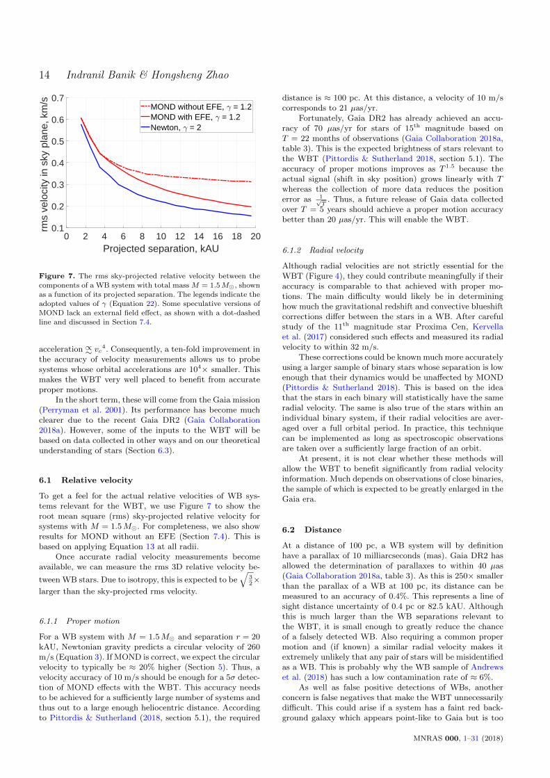
14 Indranil Banik & Hongsheng Zhao
0 2 4 6 8 10 12 14 16 18 20Projected separation, kAU
0.1
0.2
0.3
0.4
0.5
0.6
0.7
rms
velo
city
in s
ky p
lane
, km
/s
MOND without EFE, = 1.2MOND with EFE, = 1.2Newton, = 2
Figure 7. The rms sky-projected relative velocity between the
components of a WB system with total mass M = 1.5M�, shownas a function of its projected separation. The legends indicate the
adopted values of γ (Equation 22). Some speculative versions of
MOND lack an external field effect, as shown with a dot-dashedline and discussed in Section 7.4.
acceleration ∝∼ vc4. Consequently, a ten-fold improvement in
the accuracy of velocity measurements allows us to probesystems whose orbital accelerations are 104× smaller. Thismakes the WBT very well placed to benefit from accurateproper motions.
In the short term, these will come from the Gaia mission(Perryman et al. 2001). Its performance has become muchclearer due to the recent Gaia DR2 (Gaia Collaboration2018a). However, some of the inputs to the WBT will bebased on data collected in other ways and on our theoreticalunderstanding of stars (Section 6.3).
6.1 Relative velocity
To get a feel for the actual relative velocities of WB sys-tems relevant for the WBT, we use Figure 7 to show theroot mean square (rms) sky-projected relative velocity forsystems with M = 1.5M�. For completeness, we also showresults for MOND without an EFE (Section 7.4). This isbased on applying Equation 13 at all radii.
Once accurate radial velocity measurements becomeavailable, we can measure the rms 3D relative velocity be-
tween WB stars. Due to isotropy, this is expected to be√
32×
larger than the sky-projected rms velocity.
6.1.1 Proper motion
For a WB system with M = 1.5M� and separation r = 20kAU, Newtonian gravity predicts a circular velocity of 260m/s (Equation 3). If MOND is correct, we expect the circularvelocity to typically be ≈ 20% higher (Section 5). Thus, avelocity accuracy of 10 m/s should be enough for a 5σ detec-tion of MOND effects with the WBT. This accuracy needsto be achieved for a sufficiently large number of systems andthus out to a large enough heliocentric distance. Accordingto Pittordis & Sutherland (2018, section 5.1), the required
distance is ≈ 100 pc. At this distance, a velocity of 10 m/scorresponds to 21 µas/yr.
Fortunately, Gaia DR2 has already achieved an accu-racy of 70 µas/yr for stars of 15th magnitude based onT = 22 months of observations (Gaia Collaboration 2018a,table 3). This is the expected brightness of stars relevant tothe WBT (Pittordis & Sutherland 2018, section 5.1). Theaccuracy of proper motions improves as T 1.5 because theactual signal (shift in sky position) grows linearly with Twhereas the collection of more data reduces the positionerror as 1√
T. Thus, a future release of Gaia data collected
over T = 5 years should achieve a proper motion accuracybetter than 20 µas/yr. This will enable the WBT.
6.1.2 Radial velocity
Although radial velocities are not strictly essential for theWBT (Figure 4), they could contribute meaningfully if theiraccuracy is comparable to that achieved with proper mo-tions. The main difficulty would likely be in determininghow much the gravitational redshift and convective blueshiftcorrections differ between the stars in a WB. After carefulstudy of the 11th magnitude star Proxima Cen, Kervellaet al. (2017) considered such effects and measured its radialvelocity to within 32 m/s.
These corrections could be known much more accuratelyusing a larger sample of binary stars whose separation is lowenough that their dynamics would be unaffected by MOND(Pittordis & Sutherland 2018). This is based on the ideathat the stars in each binary will statistically have the sameradial velocity. The same is also true of the stars within anindividual binary system, if their radial velocities are aver-aged over a full orbital period. In practice, this techniquecan be implemented as long as spectroscopic observationsare taken over a sufficiently large fraction of an orbit.
At present, it is not clear whether these methods willallow the WBT to benefit significantly from radial velocityinformation. Much depends on observations of close binaries,the sample of which is expected to be greatly enlarged in theGaia era.
6.2 Distance
At a distance of 100 pc, a WB system will by definitionhave a parallax of 10 milliarcseconds (mas). Gaia DR2 hasallowed the determination of parallaxes to within 40 µas(Gaia Collaboration 2018a, table 3). As this is 250× smallerthan the parallax of a WB at 100 pc, its distance can bemeasured to an accuracy of 0.4%. This represents a line ofsight distance uncertainty of 0.4 pc or 82.5 kAU. Althoughthis is much larger than the WB separations relevant tothe WBT, it is small enough to greatly reduce the chanceof a falsely detected WB. Also requiring a common propermotion and (if known) a similar radial velocity makes itextremely unlikely that any pair of stars will be misidentifiedas a WB. This is probably why the WB sample of Andrewset al. (2018) has such a low contamination rate of ≈ 6%.
As well as false positive detections of WBs, anotherconcern is false negatives that make the WBT unnecessarilydifficult. This could arise if a system has a faint red back-ground galaxy which appears point-like to Gaia but is too
MNRAS 000, 1–31 (2018)
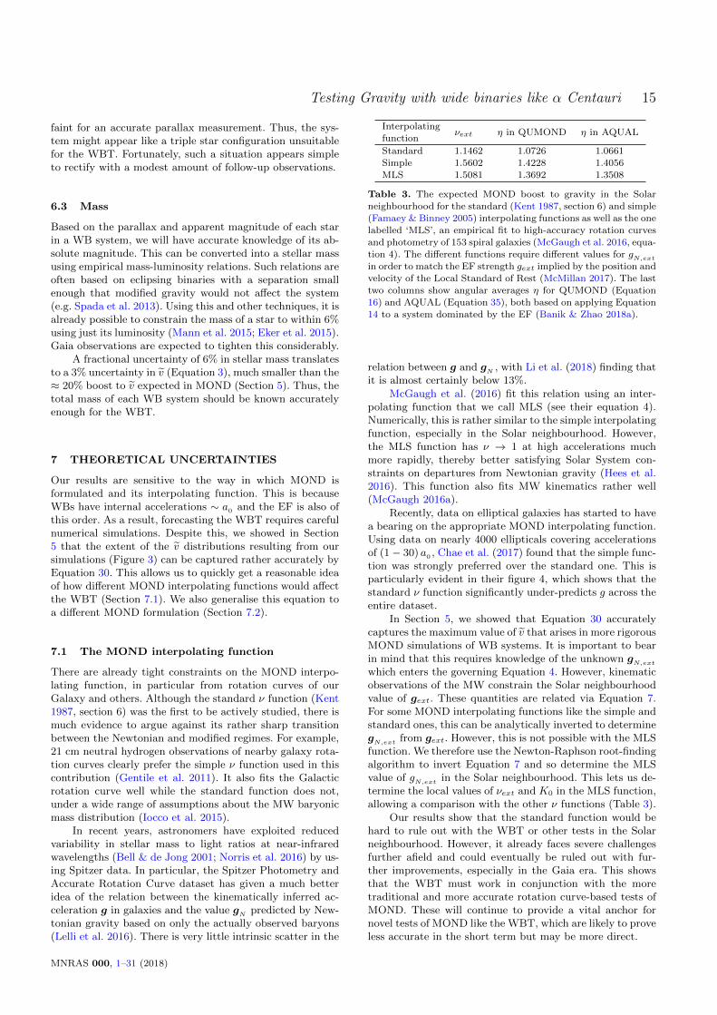
Testing Gravity with wide binaries like α Centauri 15
faint for an accurate parallax measurement. Thus, the sys-tem might appear like a triple star configuration unsuitablefor the WBT. Fortunately, such a situation appears simpleto rectify with a modest amount of follow-up observations.
6.3 Mass
Based on the parallax and apparent magnitude of each starin a WB system, we will have accurate knowledge of its ab-solute magnitude. This can be converted into a stellar massusing empirical mass-luminosity relations. Such relations areoften based on eclipsing binaries with a separation smallenough that modified gravity would not affect the system(e.g. Spada et al. 2013). Using this and other techniques, it isalready possible to constrain the mass of a star to within 6%using just its luminosity (Mann et al. 2015; Eker et al. 2015).Gaia observations are expected to tighten this considerably.
A fractional uncertainty of 6% in stellar mass translatesto a 3% uncertainty in v (Equation 3), much smaller than the≈ 20% boost to v expected in MOND (Section 5). Thus, thetotal mass of each WB system should be known accuratelyenough for the WBT.
7 THEORETICAL UNCERTAINTIES
Our results are sensitive to the way in which MOND isformulated and its interpolating function. This is becauseWBs have internal accelerations ∼ a0 and the EF is also ofthis order. As a result, forecasting the WBT requires carefulnumerical simulations. Despite this, we showed in Section5 that the extent of the v distributions resulting from oursimulations (Figure 3) can be captured rather accurately byEquation 30. This allows us to quickly get a reasonable ideaof how different MOND interpolating functions would affectthe WBT (Section 7.1). We also generalise this equation toa different MOND formulation (Section 7.2).
7.1 The MOND interpolating function
There are already tight constraints on the MOND interpo-lating function, in particular from rotation curves of ourGalaxy and others. Although the standard ν function (Kent1987, section 6) was the first to be actively studied, there ismuch evidence to argue against its rather sharp transitionbetween the Newtonian and modified regimes. For example,21 cm neutral hydrogen observations of nearby galaxy rota-tion curves clearly prefer the simple ν function used in thiscontribution (Gentile et al. 2011). It also fits the Galacticrotation curve well while the standard function does not,under a wide range of assumptions about the MW baryonicmass distribution (Iocco et al. 2015).
In recent years, astronomers have exploited reducedvariability in stellar mass to light ratios at near-infraredwavelengths (Bell & de Jong 2001; Norris et al. 2016) by us-ing Spitzer data. In particular, the Spitzer Photometry andAccurate Rotation Curve dataset has given a much betteridea of the relation between the kinematically inferred ac-celeration g in galaxies and the value gN predicted by New-tonian gravity based on only the actually observed baryons(Lelli et al. 2016). There is very little intrinsic scatter in the
Interpolatingνext η in QUMOND η in AQUAL
function
Standard 1.1462 1.0726 1.0661
Simple 1.5602 1.4228 1.4056
MLS 1.5081 1.3692 1.3508
Table 3. The expected MOND boost to gravity in the Solar
neighbourhood for the standard (Kent 1987, section 6) and simple
(Famaey & Binney 2005) interpolating functions as well as the onelabelled ‘MLS’, an empirical fit to high-accuracy rotation curves
and photometry of 153 spiral galaxies (McGaugh et al. 2016, equa-
tion 4). The different functions require different values for gN,ext
in order to match the EF strength gext implied by the position and
velocity of the Local Standard of Rest (McMillan 2017). The last
two columns show angular averages η for QUMOND (Equation16) and AQUAL (Equation 35), both based on applying Equation
14 to a system dominated by the EF (Banik & Zhao 2018a).
relation between g and gN , with Li et al. (2018) finding thatit is almost certainly below 13%.
McGaugh et al. (2016) fit this relation using an inter-polating function that we call MLS (see their equation 4).Numerically, this is rather similar to the simple interpolatingfunction, especially in the Solar neighbourhood. However,the MLS function has ν → 1 at high accelerations muchmore rapidly, thereby better satisfying Solar System con-straints on departures from Newtonian gravity (Hees et al.2016). This function also fits MW kinematics rather well(McGaugh 2016a).
Recently, data on elliptical galaxies has started to havea bearing on the appropriate MOND interpolating function.Using data on nearly 4000 ellipticals covering accelerationsof (1− 30) a0 , Chae et al. (2017) found that the simple func-tion was strongly preferred over the standard one. This isparticularly evident in their figure 4, which shows that thestandard ν function significantly under-predicts g across theentire dataset.
In Section 5, we showed that Equation 30 accuratelycaptures the maximum value of v that arises in more rigorousMOND simulations of WB systems. It is important to bearin mind that this requires knowledge of the unknown gN,ext
which enters the governing Equation 4. However, kinematicobservations of the MW constrain the Solar neighbourhoodvalue of gext. These quantities are related via Equation 7.For some MOND interpolating functions like the simple andstandard ones, this can be analytically inverted to determinegN,ext from gext. However, this is not possible with the MLSfunction. We therefore use the Newton-Raphson root-findingalgorithm to invert Equation 7 and so determine the MLSvalue of gN,ext in the Solar neighbourhood. This lets us de-termine the local values of νext and K0 in the MLS function,allowing a comparison with the other ν functions (Table 3).
Our results show that the standard function would behard to rule out with the WBT or other tests in the Solarneighbourhood. However, it already faces severe challengesfurther afield and could eventually be ruled out with fur-ther improvements, especially in the Gaia era. This showsthat the WBT must work in conjunction with the moretraditional and more accurate rotation curve-based tests ofMOND. These will continue to provide a vital anchor fornovel tests of MOND like the WBT, which are likely to proveless accurate in the short term but may be more direct.
MNRAS 000, 1–31 (2018)
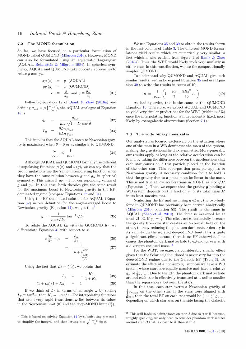
16 Indranil Banik & Hongsheng Zhao
7.2 The MOND formulation
So far, we have focused on a particular formulation ofMOND called QUMOND (Milgrom 2010). However, MONDcan also be formulated using an aquadratic Lagrangian(AQUAL, Bekenstein & Milgrom 1984). In spherical sym-metry, AQUAL and QUMOND take opposite approaches torelate g and gN .
xµ (x) = y (AQUAL)
yν (y) = x (QUMOND)
x ≡ g
a0
and y ≡ gNa0
(31)
Following equation 19 of Banik & Zhao (2018a) and
defining µext ≡ µ(gexta
0
), the AQUAL analogue of Equation
15 is
gr =gN,r
µext√
1 + L0 sin2 θ(32)
L0 ≡ ∂Lnµext
∂Ln gext
(33)
This implies that the AQUAL boost to Newtonian grav-ity is maximised when θ = 0 or π, similarly to QUMOND.
grgN,r
61
µext(34)
Although AQUAL and QUMOND formally use differentinterpolating functions µ (x) and ν (y), we can say that thetwo formulations use the ‘same’ interpolating function whenthey have the same relation between g and gN in sphericalsymmetry. This arises if µν = 1 for corresponding values ofg and gN . In this case, both theories give the same resultfor the maximum boost to Newtonian gravity in the EF-dominated regime (compare Equations 17 and 34).
Using the EF-dominated solution for AQUAL (Equa-tion 32) in our definition for the angle-averaged boost toNewtonian gravity (Equation 14), we get that1
η =1
µext√L0
tan−1√L0 (35)
To relate the AQUAL L0 with the QUMOND K0, wedifferentiate Equation 31 with respect to x.
x∂µ
∂x+ µ =
∂y
∂x(36)
=1
ν + y∂ν
∂x︸︷︷︸νK0
(37)
Using the fact that L0 = xµ∂µ∂x
, we obtain that
L0 = − K0
1 +K0(38)
(1 + L0) (1 +K0) = 1 (39)
If we think of L0 in terms of an angle ω by settingL0 ≡ tan2 ω, thenK0 = − sin2 ω. For interpolating functionsthat avoid very rapid transitions, ω lies between its valuesin the Newtonian limit (0) and the deep-MOND limit (π
4).
1 This is based on solving Equation 14 by substituting u = cos θ
to simplify the integral and then letting u =√
1+L0L0
sinφ.
We use Equations 35 and 39 to obtain the results shownin the last column of Table 3. The different MOND formu-lations yield results which are numerically very similar, afact which is also evident from figure 1 of Banik & Zhao(2018a). Thus, the WBT would likely work very similarly ineither case. In this contribution, we use the computationallysimpler QUMOND.
To understand why QUMOND and AQUAL give suchsimilar results, we Taylor expand Equation 35 and use Equa-tion 39 to write the results in terms of K0.
η =1
µext
(1 +
K0
3− 2K0
2
15. . .
)(40)
At leading order, this is the same as the QUMONDEquation 16. Therefore, we expect AQUAL and QUMONDto yield very similar predictions for the WBT (within ≈ 5%)once the interpolating function is independently fixed, mostlikely by extragalactic observations (Section 7.1).
7.3 The wide binary mass ratio
Our analysis has focused exclusively on the situation whereone of the stars in a WB dominates the mass of the system,making the gravitational field axisymmetric. More generally,our results apply as long as the relative acceleration can befound by taking the difference between the accelerations thateach star causes on a test particle placed at the locationof the other star. This superposition principle applies toNewtonian gravity. A necessary condition for it to hold isthat the gravity due to a point mass be linear in the mass.This is not true at low accelerations in MOND as g ∝
√M
(Equation 1). Thus, we expect that the gravity g binding aWB system depends on the fraction q1 of its total mass Min its least massive star.
Neglecting the EF and assuming g � a0 , the two-bodyforce in QUMOND has previously been derived analytically(Milgrom 2010, equation 53). The result is the same inAQUAL (Zhao et al. 2010). The force is weakened by atmost 21.9% if q1 = 1
2. The effect arises essentially because
the gravity from one star creates an ‘external’ field on theother, thereby reducing the phantom dark matter density inits vicinity. In the isolated deep-MOND limit, this is quitea significant effect because there is no EF otherwise. Thiscauses the phantom dark matter halo to extend for ever witha divergent enclosed mass. 2
For the WBT, we expect a considerably smaller effectgiven that the Solar neighbourhood is never very far into thedeep-MOND regime due to the Galactic EF (Table 3). Toestimate the effect of a non-zero q1 , suppose we have a WBsystem whose stars are equally massive and have a relativegN of 1
2gN,ext . Due to the EF, the phantom dark matter halo
around each star is effectively truncated at a radius smallerthan the separation r between the stars.
In this case, each star exerts a Newtonian gravity of14gN,ext on the other star. If the stars were aligned with
gext, then the total EF on each star would be(1± 1
4
)gN,ext
depending on which star was on the side facing the Galactic
2 This still leads to a finite force on star A due to star B because,roughly speaking, we only need to consider phantom dark matter
around star B that is closer to it than star A.
MNRAS 000, 1–31 (2018)
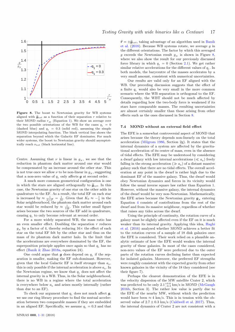
Testing Gravity with wide binaries like α Centauri 17
0 0.5 1 1.5 2 2.5 3 3.5 4 4.5 51
1.1
1.2
1.3
1.4
1.5
1.6
q1 = 0
q1 = 0.3
Figure 8. The boost to Newtonian gravity for WB systemsaligned with gext as a function of their separation r relative to
their MOND radius rM (Equation 1). We show an average over
the two possible orientations of the WB for the cases q1 = 0(dashed blue) and q1 = 0.3 (solid red), assuming the simple
MOND interpolating function. The black vertical line shows theseparation beyond which the Galactic EF dominates. For much
wider systems, the boost to Newtonian gravity should asymptot-
ically reach νext (black horizontal line).
Centre. Assuming that ν is linear in gN , we see that thereduction in phantom dark matter around one star wouldbe compensated by an increase around the other star. Thisis not true once we allow ν to be non-linear in gN , suggestingthat a non-zero value of q1 only affects g at second order.
A much more common geometrical configuration is onein which the stars are aligned orthogonally to gext. In thiscase, the Newtonian gravity of one star on the other adds inquadrature to the EF. As a result, the total EF on each staris increased by ≈ 1
2×42 = 132
. Given that K0 ≈ − 14
in theSolar neighbourhood, the phantom dark matter around eachstar would be reduced by ≈ 1
128. This rather small figure
arises because the two sources of the EF add in quadrature,causing q1 to only become relevant at second order.
For a more widely separated WB, the mass ratio hasan even smaller effect. Doubling the separation r reducesgN by a factor of 4, thereby reducing 16× the effect of eachstar on the total EF felt by the other star and thus on themass of its phantom dark matter halo. In the limit thatthe accelerations are everywhere dominated by the EF, thesuperposition principle applies once again so that q1 has noeffect (Banik & Zhao 2018a, equation 24).
One could argue that g does depend on q1 if the sep-aration is smaller, making the EF sub-dominant. However,given that the local Galactic EF is itself stronger than a0 ,this is only possible if the internal acceleration is above a0 . Inthe Newtonian regime, we know that q1 does not affect theinternal gravity in a WB. Thus, in the Solar neighbourhood,there is no WB in a regime where the total accelerationis everywhere below a0 and arises mostly internally (ratherthan due to an EF).
To check our argument that q1 does not much affect g,we use our ring library procedure to find the mutual acceler-ation between two comparable masses if they are embeddedin an aligned EF. Specifically, we assume q1 = 0.3 and that
r = ±gext, taking advantage of an algorithm used in Baniket al. (2018). Because WB systems rotate, we average g inthe different orientations. The factor by which this averagedg exceeds the Newtonian result gN is shown in Figure 8,where we also show the result for our previously discussedforce library in which q1 = 0 (Section 2.1). We get rathersimilar relative accelerations for the different values of q1 . Inboth models, the barycentre of the masses accelerates by avery small amount, consistent with numerical uncertainties.
Our results are valid only for an EF aligned with theWB. Our preceding discussion suggests that the effect ofa finite q1 would also be very small in the more commonscenario where the WB separation is orthogonal to the EF.Consequently, the WBT should not be much affected bydetails regarding how the two-body force is weakened if itsstars have comparable masses. The resulting uncertaintiesare almost certainly smaller than those arising from othereffects such as the ones discussed in Section 8.
7.4 MOND without an external field effect
The EFE is a somewhat controversial aspect of MOND thatarises because the theory depends non-linearly on the totalacceleration (Milgrom 1986, Section 2g). It states that theinternal dynamics of a system are affected by the gravita-tional acceleration of its centre of mass, even in the absenceof tidal effects. The EFE may be understood by consideringa dwarf galaxy with low internal accelerations (� a0) freelyfalling in the strong acceleration (� a0) of a distant massivegalaxy such that there are no tidal effects. The overall accel-eration at any point in the dwarf is rather high due to thedominant EF of the massive galaxy. Thus, the dwarf wouldobey Newtonian dynamics and forces in its vicinity wouldfollow the usual inverse square law rather than Equation 1.However, without the massive galaxy, the internal dynamicsof the dwarf would be very non-Newtonian. Mathematically,the EFE arises because the Newtonian gravity gN enteringEquation 4 consists of contributions from the rest of thedwarf and from its massive neighbour, regardless of whetherthat raises any tides across the dwarf.
Using the principle of continuity, the rotation curve of agalaxy must be slightly affected even if the EF on it is muchweaker than its internal gravity. Applying this idea, Haghiet al. (2016) analysed whether MOND achieves a better fitto the rotation curves of a sample of 18 disk galaxies oncethe EFE is considered. Their work relied on a plausible an-alytic estimate of how the EFE would weaken the internalgravity of these galaxies. In most of the cases considered,non-zero values of the EF were preferred due to the outerparts of the rotation curves declining faster than expectedfor isolated galaxies. Moreover, the preferred EF strengthswere roughly consistent with the expected gravity from otherknown galaxies in the vicinity of the 18 they considered (seetheir figure 7).
Perhaps the clearest demonstration of the EFE is inthe velocity dispersion of the MW satellite Crater 2, whichwas predicted to be only 2.1+0.6
−0.3 km/s in MOND (McGaugh2016b, Section 3). The rather low value is partly due tothe EFE of the nearby MW, without which the predictionwould have been ≈ 4 km/s. This is in tension with the ob-served value of 2.7± 0.3 km/s (Caldwell et al. 2017). Thus,the internal dynamics of Crater 2 are not consistent with a
MNRAS 000, 1–31 (2018)
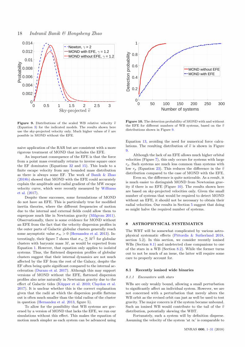
18 Indranil Banik & Hongsheng Zhao
0 0.5 1 1.5 2 2.5 30
0.002
0.004
0.006
0.008
0.01
0.012
0.014
Pro
babi
lity
Newton, = 2MOND with EFE, = 1.2MOND without EFE, = 1.2
Figure 9. Distributions of the scaled WB relative velocity v
(Equation 3) for the indicated models. The results shown here
use the sky-projected velocity only. Much higher values of v arepossible in MOND without the EFE.
naive application of the RAR but are consistent with a morerigorous treatment of MOND that includes the EFE.
An important consequence of the EFE is that the forcefrom a point mass eventually returns to inverse square oncethe EF dominates (Equations 32 and 15). This leads to afinite escape velocity from any bounded mass distributionas there is always some EF. The work of Banik & Zhao(2018b) showed that MOND with the EFE could accuratelyexplain the amplitude and radial gradient of the MW escapevelocity curve, which were recently measured by Williamset al. (2017).
Despite these successes, some formulations of MONDdo not have an EFE. This is particularly true for modifiedinertia theories, where the different frequencies of motiondue to the internal and external fields could allow them tosuperpose much like in Newtonian gravity (Milgrom 2011).Observationally, there is some evidence for MOND withoutan EFE from the fact that the velocity dispersion profiles inthe outer parts of Galactic globular clusters generally reachsome asymptotic value σ∞ > 0 (Hernandez et al. 2013). In-
terestingly, their figure 7 shows that σ∞ ∝∼M14 for globular
clusters with baryonic mass M , as would be expected fromEquation 1. However, that equation only applies to isolatedsystems. Thus, the flattened dispersion profiles of globularclusters suggest that their internal dynamics are not muchaffected by the EF from the rest of the Galaxy, despite theEF often being quite significant compared to the internal ac-celeration (Durazo et al. 2017). Although this may supportversions of MOND without the EFE, flattened dispersionprofiles also arise naturally in Newtonian gravity due to theeffect of Galactic tides (Kupper et al. 2010; Claydon et al.2017). It is unclear whether this is the correct explanationgiven that the radii at which the dispersion profile flattensout is often much smaller than the tidal radius of the clusterin question (Hernandez et al. 2013, figure 5).
To allow for the possibility that WB systems are gov-erned by a version of MOND that lacks the EFE, we run oursimulations without this effect. This makes the equation ofmotion much simpler as each system can be advanced using
0 50 100 150 200 250 300Number of systems
0
0.2
0.4
0.6
0.8
1
Det
ectio
n pr
obab
ility
MOND without EFEMOND with EFE
Figure 10. The detection probability of MOND with and without
the EFE for different numbers of WB systems, based on the v
distributions shown in Figure 9.
Equation 13, avoiding the need for numerical force calcu-lations. The resulting distribution of v is shown in Figure9.
Although the lack of an EFE allows much higher orbitalvelocities (Figure 7), this only occurs for systems with largerp. Such systems are much less common than systems withlow rp (Equation 23). This reduces the difference in the vdistribution compared to the case of MOND with the EFE.
Even so, the difference is quite noticeable. As a result, itis much easier to distinguish MOND from Newtonian grav-ity if there is no EFE (Figure 10). The results shown hereare based on sky-projected velocities only. Given the smallnumber of systems that would be required to detect MONDwithout an EFE, it should not be necessary to obtain theirradial velocities. Our results in Section 5 suggest that doingso might halve the required number of systems.
8 ASTROPHYSICAL SYSTEMATICS
The WBT will be somewhat complicated by various astro-physical systematic effects (Pittordis & Sutherland 2018,section 5.2). In this section, we consider recently ionisedWBs (Section 8.1) and undetected close companions to oneof the stars in a WB (Section 8.2). While the former turnsout to not be much of an issue, the latter will require somecare to properly account for.
8.1 Recently ionised wide binaries
8.1.1 Encounters with stars
WBs are only weakly bound, allowing a small perturbationto significantly affect an individual system. However, we arenot concerned with a perturbation that merely alters theWB orbit as the revised orbit can just as well be used to testgravity. The major concern is if the system became unbound.Such an ionised WB would contribute to the tail of the vdistribution, potentially skewing the WBT.
Fortunately, such a system will by definition disperse.Assuming the velocity of the system ‘at∞’ is comparable to
MNRAS 000, 1–31 (2018)
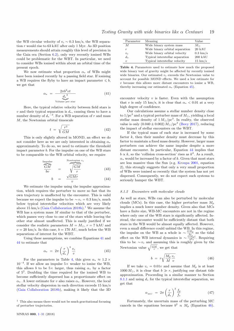
Testing Gravity with wide binaries like α Centauri 19
the WB circular velocity of vc ∼ 0.3 km/s, the WB separa-tion r would rise to 63 kAU after only 1 Myr. As 3D positionmeasurements should attain roughly this level of precision inthe Gaia era (Section 6.2), only very recently ionised WBscould be problematic for the WBT. In particular, we needto consider WBs ionised within about an orbital time of thepresent epoch.
We now estimate what proportion α∗ of WBs mighthave been ionised recently by a passing field star. If ionisinga WB requires the flyby to have an impact parameter 6 b,we get that
α∗ =2πb2vt
d∗3︸︷︷︸
Volume per star
(41)
Here, the typical relative velocity between field stars isv and their typical separation is d∗, causing them to have anumber density of d∗
−3. For a WB separation of r and massM , the Newtonian orbital timescale
t =
√r3
GM(42)
This is only slightly altered in MOND, an effect we donot consider here as we are only interested in obtaining α∗approximately. To do so, we need to estimate the thresholdimpact parameter b. For the impulse on one of the WB starsto be comparable to the WB orbital velocity, we require
Impulse︷ ︸︸ ︷GM
bv=
Newtonian vc︷ ︸︸ ︷√GM
r(43)
b =
√GMr
v(44)
We estimate the impulse using the impulse approxima-tion, which requires the perturber to move so fast that itsown trajectory is unaffected by the encounter. This is validbecause we expect the impulse to be ∼ vc = 0.3 km/s, muchbelow typical interstellar velocities which are very likelyabove 15 km/s (Gaia Collaboration 2018b).1 We assume theWB has a system mass M similar to that of the perturber,which passes very close to one of the stars while leaving theother star almost unaffected. This is easily justified if weconsider the realistic parameters M = M�, r = 7 kAU andv = 20 km/s. In this case, b = 170 AU, much below the WBseparations of interest for the WBT.
Using these assumptions, we combine Equations 41 and44 to estimate that
α∗ = 2π
(r
d∗
)3vcv
(45)
For the parameters in Table 4, this gives α∗ ≈ 1.2 ×10⁻⁴. If we allow an impulse 5× weaker to ionise the WB,this allows b to be 5× larger, thus raising α∗ by a factorof 52. Doubling the time required for the ionised WB tobecome sufficiently dispersed has a proportionate effect onα∗. A lower estimate for v also raises α∗. However, the localstellar velocity dispersion in each direction exceeds 15 km/s(Gaia Collaboration 2018b), making it likely that the 3D
1 This also means there would not be much gravitational focusing
of perturber trajectories.
Parameter Meaning Value
M Wide binary system mass M�r Wide binary orbital separation 20 kAU
vc Wide binary orbital velocity 0.3 km/s
d∗ Typical interstellar separation 200 kAUv Typical interstellar velocity 15 km/s
Table 4. Parameters used to estimate how much the proposed
wide binary test of gravity might be affected by recently ionisedwide binaries. Our estimated vc exceeds the Newtonian value to
account for possible MOND effects. We used a low estimate for
v because this allows more distant encounters to ionise a WB,thereby increasing our estimated α∗ (Equation 45).
encounter velocity v is faster. Even with the assumptionthat v is only 15 km/s, it is clear that α∗ < 0.01 at a veryhigh degree of confidence.
Our calculations assume a stellar number density closeto 1/pc3 and a typical perturber mass of M�, yielding a localstellar mass density of 1M�/pc3. In reality, the observedvalue is only (0.040± 0.002)M�/pc3 (Bovy 2017), reducingthe impact of stellar encounters on the WBT.
If the typical mass of each star is increased by somefactor k, then their number density must decrease by thisfactor to maintain a fixed mass density. However, larger massperturbers can achieve the same impulse despite a moredistant encounter. In particular, Equation 44 implies thatb ∝ k, so the ‘collision cross-section’ rises as k2. As a result,α∗ would be increased by a factor of k. Given that most starsare less massive than the Sun (e.g. Kroupa 2001, equation2), this strongly suggests that only a very small proportionof WBs were ionised so recently that the system has not yetdispersed. Consequently, we do not expect such systems toseriously hamper the WBT.
8.1.2 Encounters with molecular clouds
As well as stars, WBs can also be perturbed by molecularclouds (MCs). In this case, the higher perturber mass Mp
implies a much lower number density. Given also that MCshave a finite size, WB-MC encounters are not in the regimewhere only one of the WB stars is significantly affected. In-stead, the encounter would be sufficiently distant that bothstars in the WB would be almost equally affected. However,even a small difference could unbind the WB. In this regime,the impulse on the WB as a whole is ∼ GMp
bvso the tidal
effect on the WB internal dynamics is ∼ GMpr
b2v. Requiring
this to be ∼ vc and assuming this is roughly given by the
Newtonian value√
GMr
, we get that
b = r
√Mp
M
vcv
(46)
If we take vc = 0.01v and assume that Mp is at least1000M�, it is clear that b � r, justifying our distant tideapproximation. Proceeding in a similar manner to Section8.1.1 and using d∗ for the typical interstellar separation, weget that
αMC = 2π
(r
d∗
)3fpf∗
(47)
Fortunately, the uncertain mass of the perturbing MCcancels in the equations because b2 ∝ Mp (Equation 46).
MNRAS 000, 1–31 (2018)
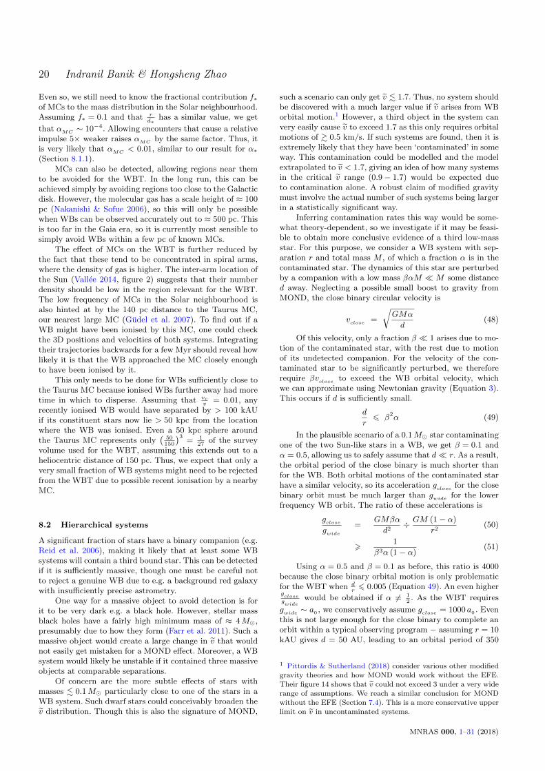
20 Indranil Banik & Hongsheng Zhao
Even so, we still need to know the fractional contribution f∗of MCs to the mass distribution in the Solar neighbourhood.Assuming f∗ = 0.1 and that r
d∗has a similar value, we get
that αMC ∼ 10−4. Allowing encounters that cause a relativeimpulse 5× weaker raises αMC by the same factor. Thus, itis very likely that αMC < 0.01, similar to our result for α∗(Section 8.1.1).
MCs can also be detected, allowing regions near themto be avoided for the WBT. In the long run, this can beachieved simply by avoiding regions too close to the Galacticdisk. However, the molecular gas has a scale height of ≈ 100pc (Nakanishi & Sofue 2006), so this will only be possiblewhen WBs can be observed accurately out to ≈ 500 pc. Thisis too far in the Gaia era, so it is currently most sensible tosimply avoid WBs within a few pc of known MCs.
The effect of MCs on the WBT is further reduced bythe fact that these tend to be concentrated in spiral arms,where the density of gas is higher. The inter-arm location ofthe Sun (Vallee 2014, figure 2) suggests that their numberdensity should be low in the region relevant for the WBT.The low frequency of MCs in the Solar neighbourhood isalso hinted at by the 140 pc distance to the Taurus MC,our nearest large MC (Gudel et al. 2007). To find out if aWB might have been ionised by this MC, one could checkthe 3D positions and velocities of both systems. Integratingtheir trajectories backwards for a few Myr should reveal howlikely it is that the WB approached the MC closely enoughto have been ionised by it.
This only needs to be done for WBs sufficiently close tothe Taurus MC because ionised WBs further away had moretime in which to disperse. Assuming that vc
v= 0.01, any
recently ionised WB would have separated by > 100 kAUif its constituent stars now lie > 50 kpc from the locationwhere the WB was ionised. Even a 50 kpc sphere aroundthe Taurus MC represents only
(50150
)3= 1
27of the survey
volume used for the WBT, assuming this extends out to aheliocentric distance of 150 pc. Thus, we expect that only avery small fraction of WB systems might need to be rejectedfrom the WBT due to possible recent ionisation by a nearbyMC.
8.2 Hierarchical systems
A significant fraction of stars have a binary companion (e.g.Reid et al. 2006), making it likely that at least some WBsystems will contain a third bound star. This can be detectedif it is sufficiently massive, though one must be careful notto reject a genuine WB due to e.g. a background red galaxywith insufficiently precise astrometry.
One way for a massive object to avoid detection is forit to be very dark e.g. a black hole. However, stellar massblack holes have a fairly high minimum mass of ≈ 4M�,presumably due to how they form (Farr et al. 2011). Such amassive object would create a large change in v that wouldnot easily get mistaken for a MOND effect. Moreover, a WBsystem would likely be unstable if it contained three massiveobjects at comparable separations.
Of concern are the more subtle effects of stars withmasses . 0.1M� particularly close to one of the stars in aWB system. Such dwarf stars could conceivably broaden thev distribution. Though this is also the signature of MOND,
such a scenario can only get v . 1.7. Thus, no system shouldbe discovered with a much larger value if v arises from WBorbital motion.1 However, a third object in the system canvery easily cause v to exceed 1.7 as this only requires orbitalmotions of & 0.5 km/s. If such systems are found, then it isextremely likely that they have been ‘contaminated’ in someway. This contamination could be modelled and the modelextrapolated to v < 1.7, giving an idea of how many systemsin the critical v range (0.9− 1.7) would be expected dueto contamination alone. A robust claim of modified gravitymust involve the actual number of such systems being largerin a statistically significant way.
Inferring contamination rates this way would be some-what theory-dependent, so we investigate if it may be feasi-ble to obtain more conclusive evidence of a third low-massstar. For this purpose, we consider a WB system with sep-aration r and total mass M , of which a fraction α is in thecontaminated star. The dynamics of this star are perturbedby a companion with a low mass βαM �M some distanced away. Neglecting a possible small boost to gravity fromMOND, the close binary circular velocity is
vclose =
√GMα
d(48)
Of this velocity, only a fraction β � 1 arises due to mo-tion of the contaminated star, with the rest due to motionof its undetected companion. For the velocity of the con-taminated star to be significantly perturbed, we thereforerequire βvclose to exceed the WB orbital velocity, whichwe can approximate using Newtonian gravity (Equation 3).This occurs if d is sufficiently small.
d
r6 β2α (49)
In the plausible scenario of a 0.1M� star contaminatingone of the two Sun-like stars in a WB, we get β = 0.1 andα = 0.5, allowing us to safely assume that d� r. As a result,the orbital period of the close binary is much shorter thanfor the WB. Both orbital motions of the contaminated starhave a similar velocity, so its acceleration gclose for the closebinary orbit must be much larger than gwide for the lowerfrequency WB orbit. The ratio of these accelerations is
gclosegwide
=GMβα
d2÷ GM (1− α)
r2(50)
>1
β3α (1− α)(51)
Using α = 0.5 and β = 0.1 as before, this ratio is 4000because the close binary orbital motion is only problematicfor the WBT when d
r6 0.005 (Equation 49). An even higher
gclosegwide
would be obtained if α 6= 12. As the WBT requires
gwide ∼ a0 , we conservatively assume gclose = 1000 a0 . Eventhis is not large enough for the close binary to complete anorbit within a typical observing program − assuming r = 10kAU gives d = 50 AU, leading to an orbital period of 350
1 Pittordis & Sutherland (2018) consider various other modifiedgravity theories and how MOND would work without the EFE.Their figure 14 shows that v could not exceed 3 under a very wide
range of assumptions. We reach a similar conclusion for MONDwithout the EFE (Section 7.4). This is a more conservative upper
limit on v in uncontaminated systems.
MNRAS 000, 1–31 (2018)
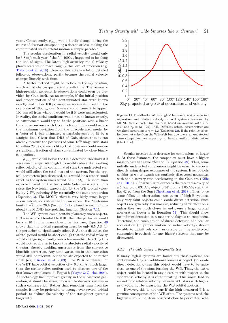
Testing Gravity with wide binaries like α Centauri 21
years. Consequently, gclose would hardly change during thecourse of observations spanning a decade or less, making thecontaminated star’s orbital motion a simple parabola.
The secular acceleration in radial velocity would onlybe 3.8 m/s each year if the full 1000a0 happened to be alongthe line of sight. The latest high-accuracy radial velocityplanet searches do reach roughly this level of precision (e.g.Trifonov et al. 2018). Even so, this entails a lot of detailedfollow-up observations, partly because the radial velocitychanges linearly with time.
A better method might be to look at the sky position,which would change quadratically with time. The necessaryhigh-precision astrometric observations could even be pro-vided by Gaia itself. As an example, if the initial positionand proper motion of the contaminated star were knownexactly and it lies 100 pc away, an acceleration within thesky plane of 1000 a0 over 5 years would cause it to appear100 µas off from where it would be if it were unaccelerated.In reality, the initial conditions would not be known exactly,so astronomers would try to fit the positions with a lineartrend in accordance with Occam’s Razor. This would reducethe maximum deviation from the unaccelerated model bya factor of 4, but ultimately a parabola can’t be fit by astraight line. Given that DR2 of Gaia shows that it canalready measure the positions of some 15th magnitude starsto within 20 µas, it seems likely that observers could removea significant fraction of stars contaminated by close binarycompanions.
gclose would fall below the Gaia detection threshold if dwere much larger. Although this would reduce the resultingreflex velocity of the contaminated star, the undetected starwould still affect the total mass of the system. For the typ-ical parameters just discussed, this would be a rather smalleffect as the system mass would be 2.1M�, 5% more thanexpected based on the two visible Solar mass stars. Thisraises the Newtonian expectation for the WB orbital veloc-ity by 2.5%, reducing v by essentially the same proportion(Equation 3). The MOND effect is very likely much larger− our calculations show that v can exceed the Newtonianlimit of
√2 by ≈ 20% (Section 5) for plausible assumptions
about the MOND interpolating function (Section 7.1).
The WB system could contain planetary mass objects.If β was reduced ten-fold to 0.01, then the perturber wouldbe a ≈ 10 Jupiter mass object. In this case, Equation 49shows that the orbital separation must be only 0.5 AU forthe perturber to significantly affect v. At this distance, theorbital period would be short enough that the radial velocitywould change significantly over a few months. Detecting thiswould not require us to know the absolute radial velocity ofthe star, thereby avoiding uncertainty from the convectiveblueshift correction. Any time variations in this correctionwould still be relevant, but these are expected to be rathersmall (e.g. Kurster et al. 2003). The WBs of interest forthe WBT have orbital velocities of ∼ 0.3 km/s, much largerthan the stellar reflex motion used to discover one of thefirst known exoplanets, 51 Pegasi b (Mayor & Queloz 1995).As technology has improved greatly in the subsequent gen-eration, it should be straightforward to discover systems insuch a configuration. Rather than removing them from thesample, it may be preferable to average over several orbitalperiods to deduce the velocity of the star-planet system’sbarycentre.
0° 20° 40° 60° 80° 100° 120° 140° 160° 180°Sky-projected angle of separation and velocity
00.20.40.60.8
11.21.41.61.8
22.2
Pro
babi
lity
Figure 11. Distribution of the angle ψ between the sky-projectedseparation and relative velocity of WB systems governed by
MOND (red curve). Our result is based on systems with v >
0.97 and rp = (3 − 20) kAU. Different orbital eccentricities areweighted according to γ = 1.2 (Equation 22). If the relative veloc-
ity does not arise from the WB orbit but due to e.g. an undetected
close companion, we expect ψ to have a uniform distribution(black line).
Secular accelerations decrease for companions at largerd. At these distances, the companion must have a highermass to have the same effect on v (Equation 49). Thus, someinitially undetected companions might be easier to discoverdirectly using deeper exposures of the system. Even objectsas faint as white dwarfs are routinely discovered nowadays,with the discovery rate accelerating in the Gaia era (Kilicet al. 2018). Of particular relevance is the recent discovery ofa 5 Gyr old 0.034M� object 0.54” from a 1.05M� star thatlies 42 pc from the Sun (Cheetham et al. 2018). Thus, oncesome follow-up observations are taken of high-v systems,only very faint objects could evade direct detection. Suchobjects are generally less massive, reducing their effect on vunless they are much closer in and cause a larger orbitalacceleration (lower β in Equation 51). This should allowfor indirect detection in a manner analogous to exoplanets.Therefore, the combination of direct detection and secularacceleration (in proper motion or radial velocity) shouldbe able to definitively confirm or rule out the undetectedcompanion hypothesis for any high-v systems that may bediscovered.
8.2.1 The wide binary orthogonality test
If many high-v systems are found but these systems arecontaminated by an additional low-mass object (to evadedirect detection), then this object would have to be quiteclose to one of the stars forming the WB. Thus, the extraobject could be located in any direction with respect to thestar whose velocity it is contaminating. This would lead toan isotropic relative velocity between WB stars with high vas v would not be measuring the WB orbital motion.
However, this is not true if the high measured v is agenuine consequence of the WB orbit. The systems with thehighest v would be those observed close to pericentre, with
MNRAS 000, 1–31 (2018)
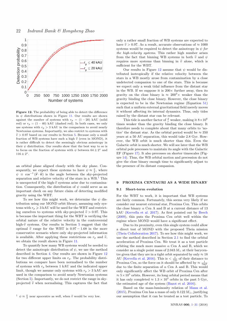
22 Indranil Banik & Hongsheng Zhao
0 250 500 750 1000 1250 1500 1750 2000Number of systems
00.10.20.30.40.50.60.70.80.9
1
Det
ectio
n pr
obab
ility
rp 40 kAU
rp 20 kAU
Figure 12. The probability of being able to detect the difference
in ψ distributions shown in Figure 11. Our results are shownagainst the number of systems with rp = (1 − 20) kAU (solid
red) or rp = (1 − 40) kAU (dashed red). In both cases, we only
use systems with rp > 3 kAU in the comparison to avoid nearlyNewtonian systems. Importantly, we also restrict to systems with
v > 0.97 based on our results in Section 5. Because only a small
fraction of WB systems have such a high v (even in MOND), itis rather difficult to detect the seemingly obvious anisotropy in
their ψ distribution. Our results show that the best way to so isto focus on the fraction of systems with ψ between 64 ± 2◦ and
116 ± 2◦.
an orbital plane aligned closely with the sky plane. Con-sequently, we expect these systems to have ψ ≈ π
2, where
ψ ≡ cos−1 (r · v) is the angle between the sky-projectedseparation and relative velocity of the stars in a WB.1 Thisis unexpected if the high-v systems arise due to contamina-tion. Consequently, the distribution of ψ could serve as animportant check on any future claim of detecting modifiedgravity using the WBT.
To see how this might work, we determine the ψ dis-tribution using our MOND orbit library, assuming only sys-tems with rp > 3 kAU will be used for the WBT and restrict-ing ourselves to systems with sky-projected v > 0.97. Thisis because the important thing for the WBT is verifying theorbital nature of the relative velocity in the controversialhigh-v systems. Our results in Section 5 suggest that theoptimal v range for the WBT is 0.97− 1.68 in the moreconservative scenario where only sky-projected informationis available. After applying these restrictions on rp and v,we obtain the result shown in Figure 11.
To quantify how many WB systems would be needed todetect the anisotropic distribution of ψ, we use the methoddescribed in Section 4. Our results are shown in Figure 12for two different upper limits on rp. The probability distri-butions we compare have been normalised to the numberof systems with rp between 1 kAU and the indicated upperlimit, though we assume only systems with rp > 3 kAU areused in the comparison to avoid nearly Newtonian systems(Section 5). Importantly, we do not restrict the range in sky-projected v when normalising. This captures the fact that
1 ψ ≈ π2
near apocentre as well, when v would be very low.
only a rather small fraction of WB systems are expected tohave v > 0.97. As a result, accurate observations of ≈ 1000systems would be required to detect the anisotropy in ψ forthe high-velocity systems. This rather high number arisesfrom the fact that binning WB systems in both v and ψrequires more systems than binning in v alone, which issufficient for the WBT.
Our results in Figure 12 assume that ψ would be dis-tributed isotropically if the relative velocity between thestars in a WB mostly arose from contamination by a closeundetected companion to one of the stars. This is becausewe expect only a weak tidal influence from the distant starin the WB. If we suppose it is 200× further away, then itsgravity on the close binary is ≈ 2002× weaker than thegravity binding the close binary. However, the close binaryis expected to be in the Newtonian regime (Equation 51)such that a uniform external gravitational field merely movesit without affecting its internal dynamics. Thus, only tidesraised by the distant star can be relevant.
This tide is another factor of dr
weaker, making it 8×10⁶
times weaker than the gravity binding the close binary. Ittherefore needs to complete about that many orbits to ‘no-tice’ the distant star. As the orbital period would be ≈ 350years at a 50 AU separation, this would take 2.8 Gyr. How-ever, the WB orbit is much shorter than this. Even theGalactic orbit is much shorter. We will see later that the WBorbital pole precesses to maintain its angle with the GalacticEF (Figure 17). It also precesses on shorter timescales (Fig-ure 14). Thus, the WB orbital motion and precession do notgive the close binary enough time to significantly adjust tothe presence of its distant companion.
9 PROXIMA CENTAURI AS A WIDE BINARY
9.1 Short-term evolution
For the WBT to work, it is important that WB systemsare fairly common. Fortunately, this seems very likely if weconsider our nearest external star, Proxima Cen. This orbitsthe close binary α Cen A and B at a current distance of 13kAU (Kervella et al. 2017). As first pointed out by Beech(2009), this puts the Proxima Cen orbit well within theregime where MOND would have a significant effect.
Due to its proximity, even this single system could allowa direct test of MOND with the proposed Theia mission(Theia Collaboration 2017). To see how this might work, weuse the method described in Section 2.1 to find the orbitalacceleration of Proxima Cen. We treat it as a test particleorbiting the much more massive α Cen A and B, which weconsider as a single point mass of 2.043M� at their barycen-tre given that they are in a tight orbit separated by only≈ 18AU (Kervella et al. 2016). This is < 1
700of their distance to
Proxima Cen, so the force on it should be affected by ≈ 17002
due to the finite separation of α Cen A and B. This wouldonly significantly affect the WB orbit of Proxima Cen after≈ 5×10⁵ orbits. However, its long orbital period means thatit has only completed ≈ 1.3× 10⁴ orbits in the past 5 Gyr,the estimated age of the system (Bazot et al. 2016).
Based on the mass-luminosity relation of Mann et al.(2015), Proxima Cen has a mass of only 0.122M�, justifyingour assumption that it can be treated as a test particle. To
MNRAS 000, 1–31 (2018)
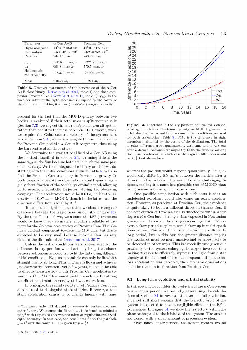
Testing Gravity with wide binaries like α Centauri 23
Parameter α Cen A+B Proxima Cen
Right ascension 14h39m40.2068s 14h29m47.7474s
Declination −60◦50′13.673′′ −62◦40′52.868′′
Parallax 747.17 mas 768.77 mas
µα,∗ -3619.9 mas/yr -3773.8 mas/yr
µδ 693.8 mas/yr 770.5 mas/yrHeliocentric
-22.332 km/s -22.204 km/sradial velocity
Mass 2.0429M� 0.1221M�
Table 5. Observed parameters of the barycentre of the α CenA+B close binary (Kervella et al. 2016, table 1) and their com-
panion Proxima Cen (Kervella et al. 2017, table 2). µα,∗ is the
time derivative of the right ascension multiplied by the cosine ofthe declination, making it a true (East-West) angular velocity.
account for the fact that the MOND gravity between twobodies is weakened if their total mass is split more equally(Section 7.3), we neglect the mass of Proxima Cen altogetherrather than add it to the mass of α Cen AB. However, whenwe require the Galactocentric velocity of the system as awhole (Section 9.3), we take a weighted mean of the valuesfor Proxima Cen and the α Cen AB barycentre, thus usingthe barycentre of all three stars.
We determine the gravitational field of α Cen AB usingthe method described in Section 2.1, assuming it feels thesame gext as the Sun because both are in much the same partof the Galaxy. We then integrate the binary orbit forwards,starting with the initial conditions given in Table 5. We alsofind the Proxima Cen trajectory in Newtonian gravity. Inboth cases, any near-term observations would span a negli-gibly short fraction of the ≈ 400 kyr orbital period, allowingus to assume a parabolic trajectory during the observingcampaign. The acceleration would be 0.60 a0 in Newtoniangravity but 0.87 a0 in MOND, though in the latter case thedirection differs from radial by 3.1◦.
To see if this might be detectable, we show the angulardifference between the trajectories on our sky (Figure 13).By the time Theia is flown, we assume the LSR parameterswould be known very accurately, allowing a reliable adjust-ment for the Galactic acceleration of Proxima Cen. This alsohas a vertical component towards the MW disk, but this isexpected to be very small because Proxima Cen lies veryclose to the disk mid-plane (Ferguson et al. 2017).
Unless the initial conditions were known exactly, thedifference in sky position would actually be 1
4that shown
because astronomers would try to fit the data using differentinitial conditions.1 Even so, a parabola can only be fit with astraight line for so long. Thus, if Theia is flown and achievesµas astrometric precision over a few years, it should be ableto directly measure how much Proxima Cen accelerates to-wards α Cen AB. This would yield a much-needed strongyet direct constraint on gravity at low accelerations.
In principle, the radial velocity vr of Proxima Cen couldalso be used to distinguish these theories. However, a con-stant acceleration causes vr to change linearly with time,
1 The exact ratio will depend on spacecraft performance and
other factors. We assume the fit to data is designed to minimise
its χ2 with respect to observations taken at regular intervals withequal accuracy. In this case, the best linear fit to the parabola
y = t2 over the range 0 − 1 is given by y = 34t.
0 2 4 6 8 10 12 14 16 18 20Time, years
02468
1012141618202224262830
Diff
eren
ce in
sky
pos
ition
, as
TotalDecRA
*
Figure 13. Difference in the sky position of Proxima Cen de-
pending on whether Newtonian gravity or MOND governs itsorbit about α Cen A and B. The same initial conditions are used
for both trajectories (Table 5). RA∗ is the difference in right
ascension multiplied by the cosine of the declination. The totalangular difference grows quadratically with time and is 7.18 µas
after a decade. Astronomers might try to fit the data by varying
the initial conditions, in which case the angular differences wouldbe ≈ 1
4that shown here.
whereas the position would respond quadratically. Thus, vrwould only differ by 0.5 cm/s between the models after adecade of observations. This would be very challenging todetect, making it a much less plausible test of MOND thanusing precise astrometry of Proxima Cen.
One possible complication with such tests is that anundetected exoplanet could also cause an extra accelera-tion. However, as perceived at Proxima Cen, the exoplanetis quite likely to be in a different direction than α Cen. Ifthe acceleration of Proxima Cen is directed to within a fewdegrees of α Cen but is stronger than expected in Newtoniangravity, then this would be strong evidence against it. More-over, a short period exoplanet would show up in multi-epochobservations. This would not be the case for a sufficientlylong period, but in this case the greater distance impliesthe exoplanet must be more massive and so more likely tobe detected in other ways. This is especially true given ourproximity to the system enlarging the angles involved, thusmaking it easier to efficiently suppress the light from a staralready at the faint end of the main sequence. If an anoma-lous acceleration was detected, then intensive observationscould be taken in its direction from Proxima Cen.
9.2 Long-term evolution and orbital stability
In this section, we consider the evolution of the α Cen systemover a longer period. We begin by generalising the calcula-tions of Section 9.1 to cover a little over one full revolution,a period still short enough that the Galactic orbit of thesystem is expected to have a negligible effect on the EF itexperiences. In Figure 14, we show the trajectory within theplane orthogonal to the initial h of the system. The orbit isnot closed, with a small amount of precession evident.
Over much longer periods, the system rotates around
MNRAS 000, 1–31 (2018)
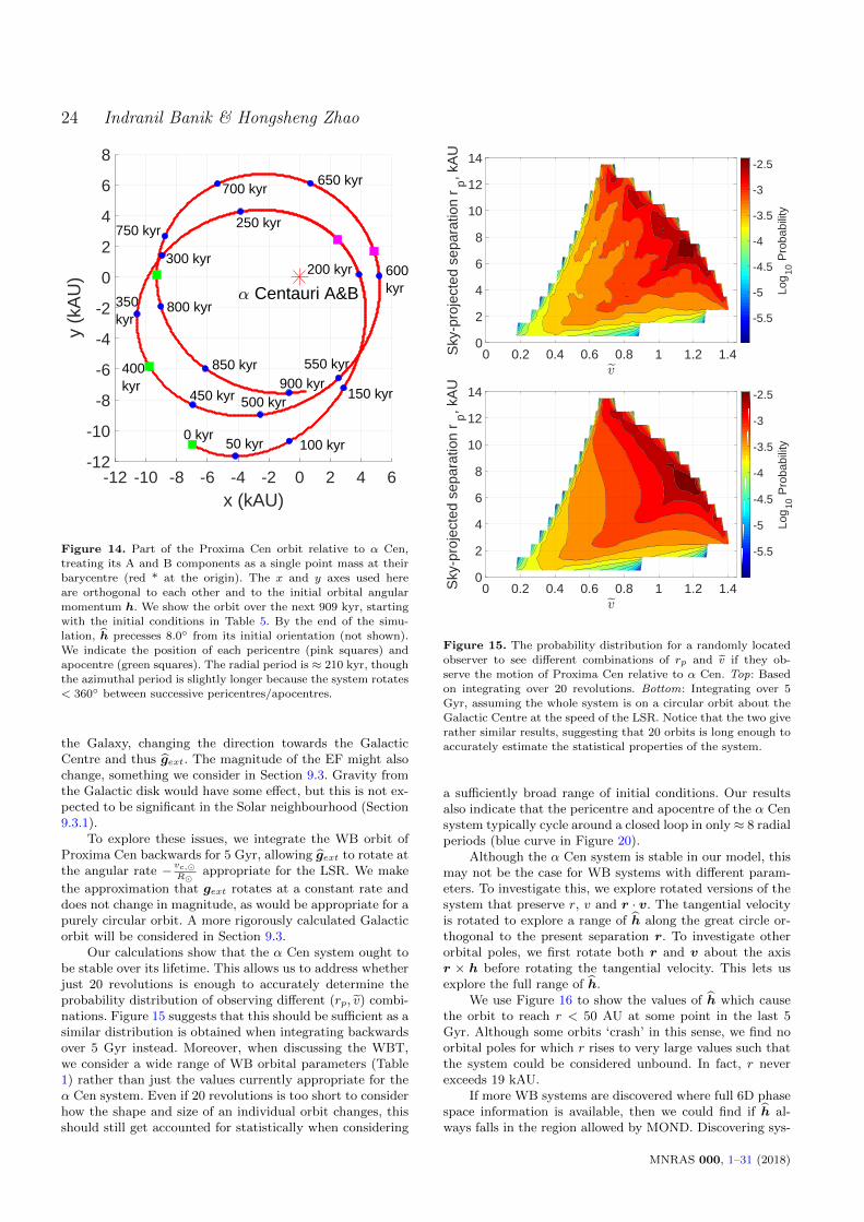
24 Indranil Banik & Hongsheng Zhao
-12 -10 -8 -6 -4 -2 0 2 4 6x (kAU)
-12
-10
-8
-6
-4
-2
0
2
4
6
8
y (k
AU
) 200 kyr300 kyr
350kyr
400kyr
500 kyr900 kyr
550 kyr
650 kyr700 kyr
0 kyr50 kyr 100 kyr
150 kyr
250 kyr
450 kyr
600kyr
750 kyr
800 kyr
850 kyr
Centauri A&B
Figure 14. Part of the Proxima Cen orbit relative to α Cen,treating its A and B components as a single point mass at their
barycentre (red * at the origin). The x and y axes used here
are orthogonal to each other and to the initial orbital angularmomentum h. We show the orbit over the next 909 kyr, starting
with the initial conditions in Table 5. By the end of the simu-
lation, h precesses 8.0◦ from its initial orientation (not shown).We indicate the position of each pericentre (pink squares) and
apocentre (green squares). The radial period is ≈ 210 kyr, thoughthe azimuthal period is slightly longer because the system rotates
< 360◦ between successive pericentres/apocentres.
the Galaxy, changing the direction towards the GalacticCentre and thus gext. The magnitude of the EF might alsochange, something we consider in Section 9.3. Gravity fromthe Galactic disk would have some effect, but this is not ex-pected to be significant in the Solar neighbourhood (Section9.3.1).
To explore these issues, we integrate the WB orbit ofProxima Cen backwards for 5 Gyr, allowing gext to rotate atthe angular rate − vc,�
R�appropriate for the LSR. We make
the approximation that gext rotates at a constant rate anddoes not change in magnitude, as would be appropriate for apurely circular orbit. A more rigorously calculated Galacticorbit will be considered in Section 9.3.
Our calculations show that the α Cen system ought tobe stable over its lifetime. This allows us to address whetherjust 20 revolutions is enough to accurately determine theprobability distribution of observing different (rp, v) combi-nations. Figure 15 suggests that this should be sufficient as asimilar distribution is obtained when integrating backwardsover 5 Gyr instead. Moreover, when discussing the WBT,we consider a wide range of WB orbital parameters (Table1) rather than just the values currently appropriate for theα Cen system. Even if 20 revolutions is too short to considerhow the shape and size of an individual orbit changes, thisshould still get accounted for statistically when considering
0 0.2 0.4 0.6 0.8 1 1.2 1.40
2
4
6
8
10
12
14
Sky
-pro
ject
ed s
epar
atio
n r p
, kA
U
-5.5
-5
-4.5
-4
-3.5
-3
-2.5
Log
10 P
roba
bilit
y
0 0.2 0.4 0.6 0.8 1 1.2 1.40
2
4
6
8
10
12
14
Sky
-pro
ject
ed s
epar
atio
n r p
, kA
U
-5.5
-5
-4.5
-4
-3.5
-3
-2.5
Log
10 P
roba
bilit
y
Figure 15. The probability distribution for a randomly located
observer to see different combinations of rp and v if they ob-serve the motion of Proxima Cen relative to α Cen. Top: Based
on integrating over 20 revolutions. Bottom: Integrating over 5
Gyr, assuming the whole system is on a circular orbit about theGalactic Centre at the speed of the LSR. Notice that the two give
rather similar results, suggesting that 20 orbits is long enough to
accurately estimate the statistical properties of the system.
a sufficiently broad range of initial conditions. Our resultsalso indicate that the pericentre and apocentre of the α Censystem typically cycle around a closed loop in only ≈ 8 radialperiods (blue curve in Figure 20).
Although the α Cen system is stable in our model, thismay not be the case for WB systems with different param-eters. To investigate this, we explore rotated versions of thesystem that preserve r, v and r · v. The tangential velocityis rotated to explore a range of h along the great circle or-thogonal to the present separation r. To investigate otherorbital poles, we first rotate both r and v about the axisr × h before rotating the tangential velocity. This lets usexplore the full range of h.
We use Figure 16 to show the values of h which causethe orbit to reach r < 50 AU at some point in the last 5Gyr. Although some orbits ‘crash’ in this sense, we find noorbital poles for which r rises to very large values such thatthe system could be considered unbound. In fact, r neverexceeds 19 kAU.
If more WB systems are discovered where full 6D phasespace information is available, then we could find if h al-ways falls in the region allowed by MOND. Discovering sys-
MNRAS 000, 1–31 (2018)
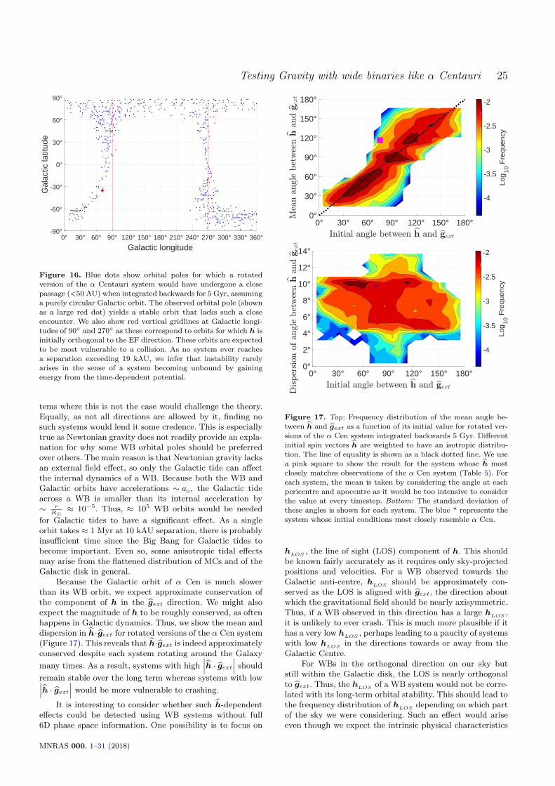
Testing Gravity with wide binaries like α Centauri 25
0° 30° 60° 90° 120° 150° 180° 210° 240° 270° 300° 330° 360°
Galactic longitude
-90°
-60°
-30°
0°
30°
60°
90°
Gal
actic
latit
ude
Figure 16. Blue dots show orbital poles for which a rotated
version of the α Centauri system would have undergone a closepassage (<50 AU) when integrated backwards for 5 Gyr, assuming
a purely circular Galactic orbit. The observed orbital pole (shown
as a large red dot) yields a stable orbit that lacks such a closeencounter. We also show red vertical gridlines at Galactic longi-
tudes of 90◦ and 270◦ as these correspond to orbits for which h is
initially orthogonal to the EF direction. These orbits are expectedto be most vulnerable to a collision. As no system ever reaches
a separation exceeding 19 kAU, we infer that instability rarely
arises in the sense of a system becoming unbound by gainingenergy from the time-dependent potential.
tems where this is not the case would challenge the theory.Equally, as not all directions are allowed by it, finding nosuch systems would lend it some credence. This is especiallytrue as Newtonian gravity does not readily provide an expla-nation for why some WB orbital poles should be preferredover others. The main reason is that Newtonian gravity lacksan external field effect, so only the Galactic tide can affectthe internal dynamics of a WB. Because both the WB andGalactic orbits have accelerations ∼ a0 , the Galactic tideacross a WB is smaller than its internal acceleration by∼ r
R�≈ 10−5. Thus, ≈ 105 WB orbits would be needed
for Galactic tides to have a significant effect. As a singleorbit takes ≈ 1 Myr at 10 kAU separation, there is probablyinsufficient time since the Big Bang for Galactic tides tobecome important. Even so, some anisotropic tidal effectsmay arise from the flattened distribution of MCs and of theGalactic disk in general.
Because the Galactic orbit of α Cen is much slowerthan its WB orbit, we expect approximate conservation ofthe component of h in the gext direction. We might alsoexpect the magnitude of h to be roughly conserved, as oftenhappens in Galactic dynamics. Thus, we show the mean anddispersion in h·gext for rotated versions of the α Cen system(Figure 17). This reveals that h·gext is indeed approximatelyconserved despite each system rotating around the Galaxy
many times. As a result, systems with high∣∣∣h · gext∣∣∣ should
remain stable over the long term whereas systems with low∣∣∣h · gext∣∣∣ would be more vulnerable to crashing.
It is interesting to consider whether such h-dependenteffects could be detected using WB systems without full6D phase space information. One possibility is to focus on
0° 30° 60° 90° 120° 150° 180°0°
30°
60°
90°
120°
150°
180°
-4
-3.5
-3
-2.5
-2
Log
10 F
requ
ency
0° 30° 60° 90° 120° 150° 180°0°
2°
4°
6°
8°
10°
12°
14°
-4
-3.5
-3
-2.5
-2
Log
10 F
requ
ency
Figure 17. Top: Frequency distribution of the mean angle be-
tween h and gext as a function of its initial value for rotated ver-sions of the α Cen system integrated backwards 5 Gyr. Different
initial spin vectors h are weighted to have an isotropic distribu-
tion. The line of equality is shown as a black dotted line. We usea pink square to show the result for the system whose h most
closely matches observations of the α Cen system (Table 5). For
each system, the mean is taken by considering the angle at eachpericentre and apocentre as it would be too intensive to consider
the value at every timestep. Bottom: The standard deviation of
these angles is shown for each system. The blue * represents thesystem whose initial conditions most closely resemble α Cen.
hLOS , the line of sight (LOS) component of h. This shouldbe known fairly accurately as it requires only sky-projectedpositions and velocities. For a WB observed towards theGalactic anti-centre, hLOS should be approximately con-served as the LOS is aligned with gext, the direction aboutwhich the gravitational field should be nearly axisymmetric.Thus, if a WB observed in this direction has a large hLOS ,it is unlikely to ever crash. This is much more plausible if ithas a very low hLOS , perhaps leading to a paucity of systemswith low hLOS in the directions towards or away from theGalactic Centre.
For WBs in the orthogonal direction on our sky butstill within the Galactic disk, the LOS is nearly orthogonalto gext. Thus, the hLOS of a WB system would not be corre-lated with its long-term orbital stability. This should lead tothe frequency distribution of hLOS depending on which partof the sky we were considering. Such an effect would ariseeven though we expect the intrinsic physical characteristics
MNRAS 000, 1–31 (2018)
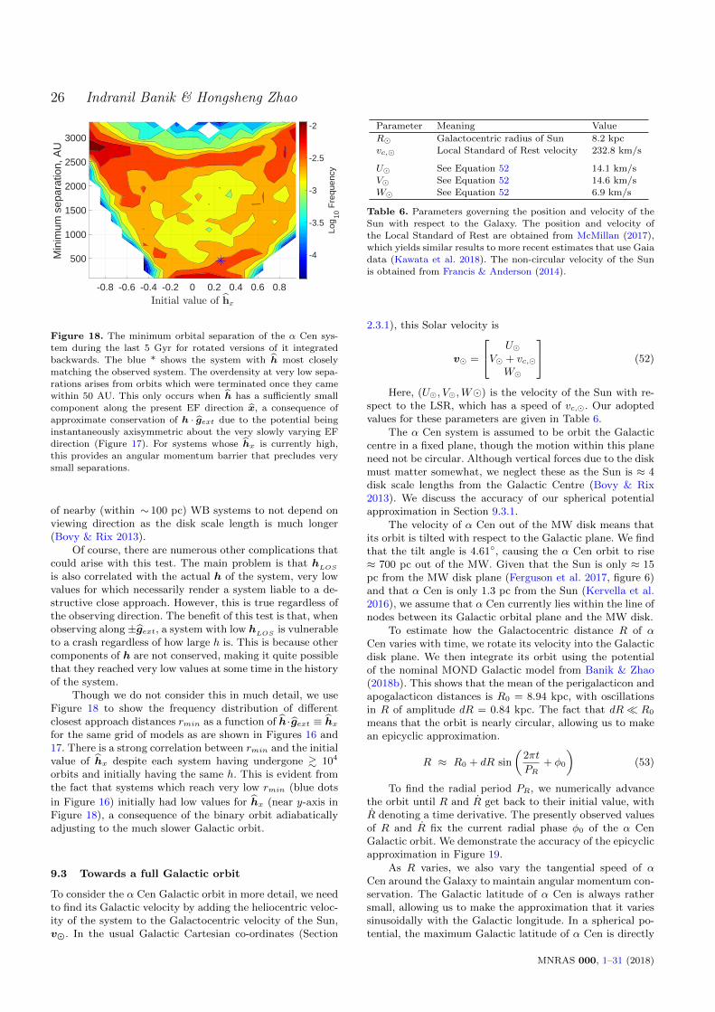
26 Indranil Banik & Hongsheng Zhao
-0.8 -0.6 -0.4 -0.2 0 0.2 0.4 0.6 0.8
500
1000
1500
2000
2500
3000
Min
imum
sep
arat
ion,
AU
-4
-3.5
-3
-2.5
-2
Log
10 F
requ
ency
Figure 18. The minimum orbital separation of the α Cen sys-
tem during the last 5 Gyr for rotated versions of it integrated
backwards. The blue * shows the system with h most closelymatching the observed system. The overdensity at very low sepa-
rations arises from orbits which were terminated once they came
within 50 AU. This only occurs when h has a sufficiently smallcomponent along the present EF direction x, a consequence of
approximate conservation of h · gext due to the potential being
instantaneously axisymmetric about the very slowly varying EFdirection (Figure 17). For systems whose hx is currently high,
this provides an angular momentum barrier that precludes very
small separations.
of nearby (within ∼ 100 pc) WB systems to not depend onviewing direction as the disk scale length is much longer(Bovy & Rix 2013).
Of course, there are numerous other complications thatcould arise with this test. The main problem is that hLOS
is also correlated with the actual h of the system, very lowvalues for which necessarily render a system liable to a de-structive close approach. However, this is true regardless ofthe observing direction. The benefit of this test is that, whenobserving along ±gext, a system with low hLOS is vulnerableto a crash regardless of how large h is. This is because othercomponents of h are not conserved, making it quite possiblethat they reached very low values at some time in the historyof the system.
Though we do not consider this in much detail, we useFigure 18 to show the frequency distribution of differentclosest approach distances rmin as a function of h·gext ≡ hxfor the same grid of models as are shown in Figures 16 and17. There is a strong correlation between rmin and the initialvalue of hx despite each system having undergone & 104
orbits and initially having the same h. This is evident fromthe fact that systems which reach very low rmin (blue dots
in Figure 16) initially had low values for hx (near y-axis inFigure 18), a consequence of the binary orbit adiabaticallyadjusting to the much slower Galactic orbit.
9.3 Towards a full Galactic orbit
To consider the α Cen Galactic orbit in more detail, we needto find its Galactic velocity by adding the heliocentric veloc-ity of the system to the Galactocentric velocity of the Sun,v�. In the usual Galactic Cartesian co-ordinates (Section
Parameter Meaning Value
R� Galactocentric radius of Sun 8.2 kpcvc,� Local Standard of Rest velocity 232.8 km/s
U� See Equation 52 14.1 km/s
V� See Equation 52 14.6 km/s
W� See Equation 52 6.9 km/s
Table 6. Parameters governing the position and velocity of the
Sun with respect to the Galaxy. The position and velocity of
the Local Standard of Rest are obtained from McMillan (2017),which yields similar results to more recent estimates that use Gaia
data (Kawata et al. 2018). The non-circular velocity of the Sun
is obtained from Francis & Anderson (2014).
2.3.1), this Solar velocity is
v� =
U�V� + vc,�
W�
(52)
Here, (U�, V�,W�) is the velocity of the Sun with re-spect to the LSR, which has a speed of vc,�. Our adoptedvalues for these parameters are given in Table 6.
The α Cen system is assumed to be orbit the Galacticcentre in a fixed plane, though the motion within this planeneed not be circular. Although vertical forces due to the diskmust matter somewhat, we neglect these as the Sun is ≈ 4disk scale lengths from the Galactic Centre (Bovy & Rix2013). We discuss the accuracy of our spherical potentialapproximation in Section 9.3.1.
The velocity of α Cen out of the MW disk means thatits orbit is tilted with respect to the Galactic plane. We findthat the tilt angle is 4.61◦, causing the α Cen orbit to rise≈ 700 pc out of the MW. Given that the Sun is only ≈ 15pc from the MW disk plane (Ferguson et al. 2017, figure 6)and that α Cen is only 1.3 pc from the Sun (Kervella et al.2016), we assume that α Cen currently lies within the line ofnodes between its Galactic orbital plane and the MW disk.
To estimate how the Galactocentric distance R of αCen varies with time, we rotate its velocity into the Galacticdisk plane. We then integrate its orbit using the potentialof the nominal MOND Galactic model from Banik & Zhao(2018b). This shows that the mean of the perigalacticon andapogalacticon distances is R0 = 8.94 kpc, with oscillationsin R of amplitude dR = 0.84 kpc. The fact that dR� R0
means that the orbit is nearly circular, allowing us to makean epicyclic approximation.
R ≈ R0 + dR sin
(2πt
PR+ φ0
)(53)
To find the radial period PR, we numerically advancethe orbit until R and R get back to their initial value, withR denoting a time derivative. The presently observed valuesof R and R fix the current radial phase φ0 of the α CenGalactic orbit. We demonstrate the accuracy of the epicyclicapproximation in Figure 19.
As R varies, we also vary the tangential speed of αCen around the Galaxy to maintain angular momentum con-servation. The Galactic latitude of α Cen is always rathersmall, allowing us to make the approximation that it variessinusoidally with the Galactic longitude. In a spherical po-tential, the maximum Galactic latitude of α Cen is directly
MNRAS 000, 1–31 (2018)
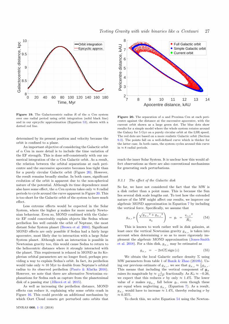
Testing Gravity with wide binaries like α Centauri 27
0 20 40 60 80 100 120 140 160 180Time, Myr
8
8.5
9
9.5
10
Gal
acto
cent
ric d
ista
nce,
kpc Orbit integration
Epicyclic approx.
Figure 19. The Galactocentric radius R of the α Cen system
over one radial period using orbit integration (solid black line)and in our epicyclic approximation (Equation 53), shown with a
dotted red line.
determined by its present position and velocity because theorbit is confined to a plane.
An important objective of considering the Galactic orbitof α Cen in more detail is to include the time variation ofthe EF strength. This is done self-consistently with our nu-merical integration of the α Cen Galactic orbit. As a result,the relation between the orbital separations at each peri-centre and the successive apocentre becomes less tight thanfor a purely circular Galactic orbit (Figure 20). However,the result remains broadly similar. In both cases, significantevolution of the orbit is apparent due to the non-sphericalnature of the potential. Although its time dependence mustalso have some effect, the α Cen system takes only ≈ 8 radialperiods to cycle around the curve apparent in Figure 20. Thisis too short for the Galactic orbit of the system to have mucheffect.
Less extreme effects would be expected in the SolarSystem, where the higher g makes for more nearly Newto-nian behaviour. Even so, MOND combined with the Galac-tic EF could conceivably explain objects like Sedna whoseperihelion lies well outside the orbit of Neptune, the mostdistant Solar System planet (Brown et al. 2004). SignificantMOND effects are only possible if Sedna had a fairly largeapocentre, most likely due to interaction with a large SolarSystem planet. Although such an interaction is possible inNewtonian gravity too, this would cause Sedna to return tothe heliocentric distance where it strongly interacted withthe planet. This requirement is relaxed in MOND as its Ke-plerian orbital parameters are no longer fixed, perhaps pro-viding a way to explain Sedna’s orbit. In fact, its perihelionwould take only ≈ 10 Myr to double from Neptune’s orbitalradius to its observed perihelion (Pauco & Klacka 2016).However, we note that there are alternative Newtonian ex-planations for Sedna such as capture from the planetesimaldisk of a passing star (Jılkova et al. 2015).
As well as increasing the perihelion distance, MONDeffects can reduce it, explaining why some orbits crash inFigure 16. This could provide an additional mechanism bywhich Oort Cloud comets get perturbed onto orbits that
7 8 9 10 11 12 13 14Apocentre distance, kAU
2
3
4
5
6
7
8
Per
icen
tre
dist
ance
, kA
U Full Galactic orbitSimple Galactic orbitCurrent orbit
Figure 20. The separation of α and Proxima Cen at each peri-
centre against the distance at the successive apocentre, with the
current orbit shown as a large green dot. The blue dots showresults for a simple model where the whole system rotates around
the Galaxy for 5 Gyr on a purely circular orbit at the LSR speed.
The red dots are based on a more realistic Galactic orbit (Section9.3). The points fall on a well-defined curve which is thicker for
the latter case. In both cases, the system cycles around this curve
in ≈ 8 radial periods.
reach the inner Solar System. It is unclear how this would af-fect observations as there are also conventional mechanismsfor generating such perturbations.
9.3.1 The effect of the Galactic disk
So far, we have not considered the fact that the MW isa disk rather than a point mass. This is because the Sunlies several disk scale lengths out. To test how the extendednature of the MW might affect our results, we improve ouralgebraic MOND approximation in Equation 7 by includingthe vertical force. Specifically, we assume that
gN,r ν
(√gN,r
2 + gN,z2
a0
)= gr =
vc,�2
R�(54)
This is known to work rather well in disk galaxies, atleast once the vertical Newtonian gravity gN,z is taken intoaccount when determining ν so as to more rigorously im-plement the algebraic MOND approximation (Jones-Smithet al. 2018). For a thin disk, gN,z may be estimated as
gN,z = − 2πGΣ sign (z) (55)
We obtain the local Galactic surface density Σ usingMW parameters from table 1 of Banik & Zhao (2018b). Us-ing our previous estimate of gN,r , we see that gN,z ≈ 1
3gN,r .
This means that including the vertical component of gN
raises its magnitude by ≈ 12×32 fractionally. As K0 ≈ −0.26,
we expect that this reduces ν by only ≈ 1.4%. The lowervalue of ν makes νgN,r fall below gr, even though theseare equal when neglecting gN,z (Equation 7). As a result,gN,r would have to increase ≈ 1.4%, thereby reducing ν by≈ 0.35%.
To check this, we solve Equation 54 using the Newton-
MNRAS 000, 1–31 (2018)
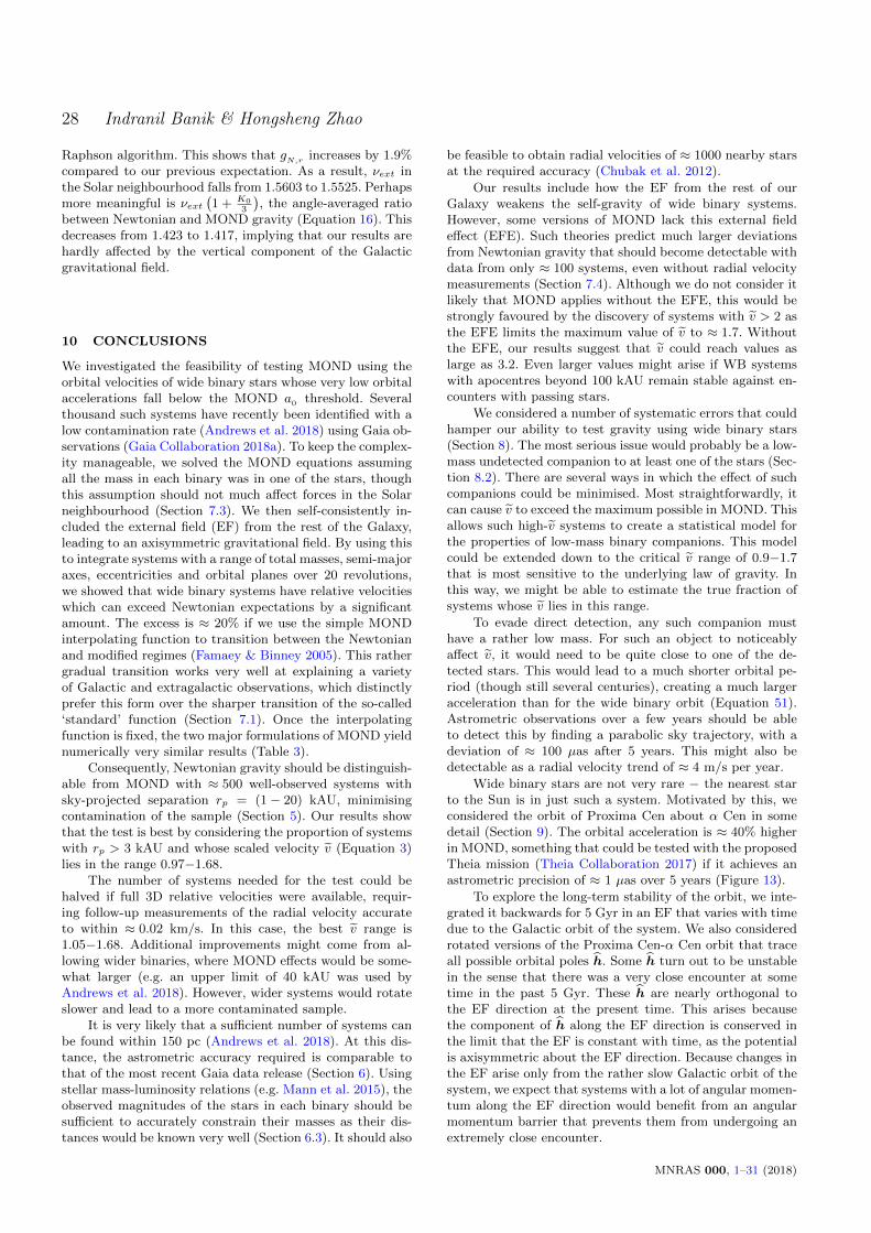
28 Indranil Banik & Hongsheng Zhao
Raphson algorithm. This shows that gN,r increases by 1.9%compared to our previous expectation. As a result, νext inthe Solar neighbourhood falls from 1.5603 to 1.5525. Perhapsmore meaningful is νext
(1 + K0
3
), the angle-averaged ratio
between Newtonian and MOND gravity (Equation 16). Thisdecreases from 1.423 to 1.417, implying that our results arehardly affected by the vertical component of the Galacticgravitational field.
10 CONCLUSIONS
We investigated the feasibility of testing MOND using theorbital velocities of wide binary stars whose very low orbitalaccelerations fall below the MOND a0 threshold. Severalthousand such systems have recently been identified with alow contamination rate (Andrews et al. 2018) using Gaia ob-servations (Gaia Collaboration 2018a). To keep the complex-ity manageable, we solved the MOND equations assumingall the mass in each binary was in one of the stars, thoughthis assumption should not much affect forces in the Solarneighbourhood (Section 7.3). We then self-consistently in-cluded the external field (EF) from the rest of the Galaxy,leading to an axisymmetric gravitational field. By using thisto integrate systems with a range of total masses, semi-majoraxes, eccentricities and orbital planes over 20 revolutions,we showed that wide binary systems have relative velocitieswhich can exceed Newtonian expectations by a significantamount. The excess is ≈ 20% if we use the simple MONDinterpolating function to transition between the Newtonianand modified regimes (Famaey & Binney 2005). This rathergradual transition works very well at explaining a varietyof Galactic and extragalactic observations, which distinctlyprefer this form over the sharper transition of the so-called‘standard’ function (Section 7.1). Once the interpolatingfunction is fixed, the two major formulations of MOND yieldnumerically very similar results (Table 3).
Consequently, Newtonian gravity should be distinguish-able from MOND with ≈ 500 well-observed systems withsky-projected separation rp = (1− 20) kAU, minimisingcontamination of the sample (Section 5). Our results showthat the test is best by considering the proportion of systemswith rp > 3 kAU and whose scaled velocity v (Equation 3)lies in the range 0.97−1.68.
The number of systems needed for the test could behalved if full 3D relative velocities were available, requir-ing follow-up measurements of the radial velocity accurateto within ≈ 0.02 km/s. In this case, the best v range is1.05−1.68. Additional improvements might come from al-lowing wider binaries, where MOND effects would be some-what larger (e.g. an upper limit of 40 kAU was used byAndrews et al. 2018). However, wider systems would rotateslower and lead to a more contaminated sample.
It is very likely that a sufficient number of systems canbe found within 150 pc (Andrews et al. 2018). At this dis-tance, the astrometric accuracy required is comparable tothat of the most recent Gaia data release (Section 6). Usingstellar mass-luminosity relations (e.g. Mann et al. 2015), theobserved magnitudes of the stars in each binary should besufficient to accurately constrain their masses as their dis-tances would be known very well (Section 6.3). It should also
be feasible to obtain radial velocities of ≈ 1000 nearby starsat the required accuracy (Chubak et al. 2012).
Our results include how the EF from the rest of ourGalaxy weakens the self-gravity of wide binary systems.However, some versions of MOND lack this external fieldeffect (EFE). Such theories predict much larger deviationsfrom Newtonian gravity that should become detectable withdata from only ≈ 100 systems, even without radial velocitymeasurements (Section 7.4). Although we do not consider itlikely that MOND applies without the EFE, this would bestrongly favoured by the discovery of systems with v > 2 asthe EFE limits the maximum value of v to ≈ 1.7. Withoutthe EFE, our results suggest that v could reach values aslarge as 3.2. Even larger values might arise if WB systemswith apocentres beyond 100 kAU remain stable against en-counters with passing stars.
We considered a number of systematic errors that couldhamper our ability to test gravity using wide binary stars(Section 8). The most serious issue would probably be a low-mass undetected companion to at least one of the stars (Sec-tion 8.2). There are several ways in which the effect of suchcompanions could be minimised. Most straightforwardly, itcan cause v to exceed the maximum possible in MOND. Thisallows such high-v systems to create a statistical model forthe properties of low-mass binary companions. This modelcould be extended down to the critical v range of 0.9−1.7that is most sensitive to the underlying law of gravity. Inthis way, we might be able to estimate the true fraction ofsystems whose v lies in this range.
To evade direct detection, any such companion musthave a rather low mass. For such an object to noticeablyaffect v, it would need to be quite close to one of the de-tected stars. This would lead to a much shorter orbital pe-riod (though still several centuries), creating a much largeracceleration than for the wide binary orbit (Equation 51).Astrometric observations over a few years should be ableto detect this by finding a parabolic sky trajectory, with adeviation of ≈ 100 µas after 5 years. This might also bedetectable as a radial velocity trend of ≈ 4 m/s per year.
Wide binary stars are not very rare − the nearest starto the Sun is in just such a system. Motivated by this, weconsidered the orbit of Proxima Cen about α Cen in somedetail (Section 9). The orbital acceleration is ≈ 40% higherin MOND, something that could be tested with the proposedTheia mission (Theia Collaboration 2017) if it achieves anastrometric precision of ≈ 1 µas over 5 years (Figure 13).
To explore the long-term stability of the orbit, we inte-grated it backwards for 5 Gyr in an EF that varies with timedue to the Galactic orbit of the system. We also consideredrotated versions of the Proxima Cen-α Cen orbit that traceall possible orbital poles h. Some h turn out to be unstablein the sense that there was a very close encounter at sometime in the past 5 Gyr. These h are nearly orthogonal tothe EF direction at the present time. This arises becausethe component of h along the EF direction is conserved inthe limit that the EF is constant with time, as the potentialis axisymmetric about the EF direction. Because changes inthe EF arise only from the rather slow Galactic orbit of thesystem, we expect that systems with a lot of angular momen-tum along the EF direction would benefit from an angularmomentum barrier that prevents them from undergoing anextremely close encounter.
MNRAS 000, 1–31 (2018)
Testing Gravity with wide binaries like α Centauri 29
Systems like this are indeed generally stable, with theminimum separation well correlated with the fraction of theangular momentum that presently lies along the EF direc-tion (Figure 18). Moreover, the angle between h and theEF is conserved rather well despite the systems completingmany Galactic orbits that completely reorient the EF (Fig-ure 17). This suggests that we may gain a deeper analyticunderstanding of wide binaries by assuming that the binaryorbit adjusts adiabatically to the much slower Galactic orbit.The dependence of orbital stability on h could also providea basis for testing MOND using novel direction-dependenteffects (Section 9.2).
Wide binary stars promise to be an exciting new fron-tier in the quest to understand the law of gravity relevantto low-acceleration astrophysical systems like galaxies. Suchunderstanding almost certainly requires non-galactic tests ofthe gravity law, an area that has received little attention sofar. Wide binary systems promise to provide just such a test,perhaps using the catalogue of such systems identified byAndrews et al. (2018) based on the Gaia mission (Perrymanet al. 2001). Although Gaia has already released data onmore than a billion stars (Gaia Collaboration 2018a), precisedata on only a minute fraction of them should be sufficientto answer fundamental questions about the laws governingour Universe.
11 ACKNOWLEDGEMENTS
IB was partially supported by Science and Technology Fa-cilities Council studentship 1506672. He is grateful to theWeizmann Institute of Science for hosting him during aweek-long visit. During this visit, he had some very helpfuldiscussions with Mordehai Milgrom, Boaz Katz and DoronKushnir that greatly advanced this contribution. He alsothanks Will Sutherland for providing an observational per-spective and Duncan Forgan for comments on tides. Theauthors wish to thank the referee for comments which im-proved this manuscript.
REFERENCES
Alcock C., et al., 2000, ApJ, 542, 281
Andrews J. J., Chaname J., Agueros M. A., 2017, MNRAS, 472,675
Andrews J. J., Chaname J., Agueros M. A., 2018, Research Notes
of the American Astronomical Society, 2, 29
Bahcall J. N., Hut P., Tremaine S., 1985, ApJ, 290, 15
Banik I., Zhao H., 2016, MNRAS, 459, 2237
Banik I., Zhao H., 2017, MNRAS, 467, 2180
Banik I., Zhao H., 2018a, SciFed Journal of Astrophysics, 1,
1000008
Banik I., Zhao H., 2018b, MNRAS, 473, 419
Banik I., Zhao H., 2018c, MNRAS, 473, 4033
Banik I., O’Ryan D., Zhao H., 2018, MNRAS, 477, 4768
Barnes J. E., Hernquist L., 1992, Nature, 360, 715
Bazot M., Christensen-Dalsgaard J., Gizon L., Benomar O., 2016,MNRAS, 460, 1254
Beech M., 2009, MNRAS, 399, L21
Beech M., 2011, ApSS, 333, 419
Bekenstein J., Milgrom M., 1984, ApJ, 286, 7
Bell E. F., de Jong R. S., 2001, ApJ, 550, 212
Belloni D., Askar A., Giersz M., Kroupa P., Rocha-Pinto H. J.,
2017, MNRAS, 471, 2812
Belokurov V., Erkal D., Evans N. W., Koposov S. E., Deason
A. J., 2018, MNRAS, 478, 611
Bershady M. A., Verheijen M. A. W., Swaters R. A., AndersenD. R., Westfall K. B., Martinsson T., 2010, ApJ, 716, 198
Bılek M., Thies I., Kroupa P., Famaey B., 2018, A&A, 614, A59
Binney J., Tremaine S., 2008, Galactic Dynamics: Second Edition.
Princeton University Press
Bovy J., 2017, MNRAS, 470, 1360
Bovy J., Rix H.-W., 2013, ApJ, 779, 115
Brada R., Milgrom M., 1999, ApJ, 519, 590
Brown M. E., Trujillo C., Rabinowitz D., 2004, ApJ, 617, 645
Caldwell N., et al., 2017, ApJ, 839, 20
Chae K.-H., Bernardi M., Sheth R. K., 2017, preprint, Arxiv
(arXiv:1707.08280)
Cheetham A., et al., 2018, A&A, 614, A16
Chubak C., Marcy G., Fischer D. A., Howard A. W., Isaac-
son H., Johnson J. A., Wright J. T., 2012, preprint, Arxiv(arXiv:1207.6212)
Claydon I., Gieles M., Zocchi A., 2017, MNRAS, 466, 3937
D’Onghia E., 2015, ApJL, 808, L8
Desmond H., 2017a, MNRAS, 464, 4160
Desmond H., 2017b, MNRAS, 472, L35
Dubinski J., Gauthier J.-R., Widrow L., Nickerson S., 2008, in
Funes J. G., Corsini E. M., eds, Astronomical Society of the
Pacific Conference Series Vol. 396, Formation and Evolutionof Galaxy Disks. p. 321 (arXiv:0802.3997)
Durazo R., Hernandez X., Cervantes Sodi B., Sanchez S. F., 2017,ApJ, 837, 179
Eker Z., et al., 2015, AJ, 149, 131
Fall S. M., Lynden-Bell D., 1981, The structure and evolution ofnormal galaxies. NATO Advanced Study Institute held at the
Institute of Astronomy and Clare College, Cambridge, UK, 3
- 15 August 1980.. Cambridge University Press
Famaey B., Binney J., 2005, MNRAS, 363, 603
Famaey B., McGaugh S. S., 2012, Living Reviews in Relativity,15, 10
Farr W. M., Sravan N., Cantrell A., Kreidberg L., Bailyn C. D.,
Mandel I., Kalogera V., 2011, ApJ, 741, 103
Feng F., Jones H. R. A., 2018, MNRAS, 473, 3185
Ferguson D., Gardner S., Yanny B., 2017, ApJ, 843, 141
Forero-Romero J. E., Arias V., 2018, MNRAS, 478, 5538
Francis C., Anderson E., 2014, Celestial Mechanics and Dynami-cal Astronomy, 118, 399
Fuchs B., 2003, ApSS, 284, 719
Gaia Collaboration 2018b, A&A, forthcoming
Gaia Collaboration 2018a, A&A, forthcoming
Gentile G., Famaey B., de Blok W. J. G., 2011, A&A, 527, A76
Gilmore G., Reid N., 1983, MNRAS, 202, 1025
Gudel M., et al., 2007, A&A, 468, 353
Haghi H., Bazkiaei A. E., Zonoozi A. H., Kroupa P., 2016, MN-RAS, 458, 4172
Hees A., Famaey B., Angus G. W., Gentile G., 2016, MNRAS,455, 449
Hernandez X., Jimenez M. A., Allen C., 2012, European PhysicalJournal C, 72, 1884
Hernandez X., Jimenez M. A., Allen C., 2013, MNRAS, 428, 3196
Hohl F., 1971, ApJ, 168, 343
Hu S., Sijacki D., 2018, MNRAS, 478, 1576
Ibata R. A., et al., 2013, Nature, 493, 62
Iocco F., Pato M., Bertone G., 2015, Physical Review D, 92,
084046
Jiang Y.-F., Tremaine S., 2010, MNRAS, 401, 977
Jılkova L., Portegies Zwart S., Pijloo T., Hammer M., 2015, MN-
RAS, 453, 3157
Jones-Smith K., Abraham R., Kell L., Mathur H., 2018, NewJournal of Physics, 20, 063042
MNRAS 000, 1–31 (2018)
30 Indranil Banik & Hongsheng Zhao
Kahn F. D., Woltjer L., 1959, ApJ, 130, 705
Kaib N. A., Raymond S. N., 2014, ApJ, 782, 60
Kawata D., Bovy J., Matsunaga N., Baba J., 2018, preprint, Arxiv
(arXiv:1803.05927)
Kent S. M., 1987, AJ, 93, 816
Kervella P., Mignard F., Merand A., Thevenin F., 2016, A&A,
594, A107
Kervella P., Thevenin F., Lovis C., 2017, A&A, 598, L7
Kilic M., Hambly N. C., Bergeron P., Genest-Beaulieu C., RowellN., 2018, MNRAS, forthcoming
Kroupa P., 2001, MNRAS, 322, 231
Kroupa P., Theis C., Boily C. M., 2005, A&A, 431, 517
Kupper A. H. W., Kroupa P., Baumgardt H., Heggie D. C., 2010,
MNRAS, 407, 2241
Kurster M., et al., 2003, A&A, 403, 1077
Lee J., 2018, ApJ, 856, 57
Lee J., Li B., 2017, ApJ, 842, 2
Lee J., Kim S., Rey S.-C., 2015, ApJ, 815, 43
Lelli F., McGaugh S. S., Schombert J. M., 2016, AJ, 152, 157
Lelli F., McGaugh S. S., Schombert J. M., Pawlowski M. S., 2017,ApJ, 836, 152
Lepine S., Bongiorno B., 2007, AJ, 133, 889
Li P., Lelli F., McGaugh S., Schombert J., 2018, A&A, forthcom-
ing
Lin C. C., Shu F. H., 1964, ApJ, 140, 646
Mann A. W., Feiden G. A., Gaidos E., Boyajian T., von Braun
K., 2015, ApJ, 804, 64
Mayor M., Queloz D., 1995, Nature, 378, 355
McGaugh S. S., 2011, Physical Review Letters, 106, 121303
McGaugh S. S., 2016a, ApJ, 816, 42
McGaugh S. S., 2016b, ApJL, 832, L8
McGaugh S., Milgrom M., 2013a, ApJ, 775, 139
McGaugh S., Milgrom M., 2013b, ApJ, 775, 139
McGaugh S. S., Wolf J., 2010, ApJ, 722, 248
McGaugh S. S., Schombert J. M., Bothun G. D., 1995, AJ, 109,2019
McGaugh S., Lelli F., Schombert J., 2016, Phys. Rev. Lett., 117,
201101
McMillan P. J., 2017, MNRAS, 465, 76
Milgrom M., 1983, ApJ, 270, 365
Milgrom M., 1986, ApJ, 302, 617
Milgrom M., 1989, ApJ, 338, 121
Milgrom M., 1999, Phys. Lett. A, 253, 273
Milgrom M., 2010, MNRAS, 403, 886
Milgrom M., 2011, Acta Physica Polonica B, 42, 2175
Mirabel I. F., Dottori H., Lutz D., 1992, A&A, 256, L19
Muller O., Pawlowski M. S., Jerjen H., Lelli F., 2018, Science,359, 534
Nakanishi H., Sofue Y., 2006, PASJ, 58, 847
Norris M. A., et al., 2016, ApJ, 832, 198
Ostriker J. P., Peebles P. J. E., 1973, ApJ, 186, 467
Ostriker J. P., Steinhardt P. J., 1995, Nature, 377, 600
Pauco R., Klacka J., 2017, preprint, Arxiv (arXiv:1705.09273)
Pauco R., Klacka J., 2016, A&A, 589
Pawlowski M. S., 2018, Modern Physics Letters A, 33, 1830004
Pazy E., 2013, Phys. Rev. D, 87, 084063
Peebles P. J. E., 2017, preprint, Arxiv (arXiv:1705.10683)
Perryman M. A. C., et al., 2001, A&A, 369, 339
Peters P. C., 1981, American Journal of Physics, 49, 564
Peters W., Kuzio de Naray R., 2018, MNRAS, 476, 2938
Pittordis C., Sutherland W., 2018, MNRAS, forthcoming
Reid I. N., Lewitus E., Allen P. R., Cruz K. L., Burgasser A. J.,2006, AJ, 132, 891
Riess A. G., et al., 1998, AJ, 116, 1009
Rogstad D. H., Shostak G. S., 1972, ApJ, 176, 315
Rowland D. R., 2015, International Journal of Modern PhysicsD, 24, 1550065
Saburova A. S., 2011, Astronomy Reports, 55, 409
Salucci P., Turini N., 2017, preprint, Arxiv (arXiv:1707.01059)
Scarpa R., Ottolina R., Falomo R., Treves A., 2017, InternationalJournal of Modern Physics D, 26, 1750067
Schutz K., Lin T., Safdi B. R., Wu C.-L., 2017, preprint, Arxiv
(arXiv:1711.03103)
Shao S., Cautun M., Frenk C. S., Grand R. J. J., Gomez F. A.,
Marinacci F., Simpson C. M., 2018, MNRAS, 476, 1796
Shaya E. J., Olling R. P., 2011, ApJS, 192, 2
Smolin L., 2017, Physical Review D, 96, 083523
Spada F., Demarque P., Kim Y.-C., Sills A., 2013, ApJ, 776, 87
Theia Collaboration 2017, preprint, Arxiv (arXiv:1707.01348)
Tisserand P., et al., 2007, A&A, 469, 387
Tokovinin A., 2017, MNRAS, 468, 3461
Tokovinin A., Kiyaeva O., 2016, MNRAS, 456, 2070
Toomre A., 1964, ApJ, 139, 1217
Trifonov T., et al., 2018, A&A, 609, A117
Vallee J. P., 2014, AJ, 148, 5
Vallee J. P., 2017, ApSS, 362, 79
Verlinde E. P., 2016, SciPost Physics, 2, 16
Wetzstein M., Naab T., Burkert A., 2007, MNRAS, 375, 805
Williams A. A., Belokurov V., Casey A. R., Evans N. W., 2017,
MNRAS, 468, 2359
Yu J., Liu C., 2018, MNRAS, 475, 1093
Zhao H., Li B., Bienayme O., 2010, Physical Review D, 82, 103001
Zhao H., Famaey B., Lughausen F., Kroupa P., 2013, A&A, 557,
L3
Zwicky F., 1937, ApJ, 86, 217
de Almeida A. O. F., Piattella O. F., Rodrigues D. C., 2016,
MNRAS, 462, 2706
den Heijer M., et al., 2015, A&A, 581, A98
van Leeuwen F., 2007, A&A, 474, 653
APPENDIX A: DERIVATION OF EQUATION 11
In this section, we determine the contribution to the poten-tial at the point (r, θ) arising from phantom dark matterexterior to the radius rout > r relative to a point massM embedded in a uniform external field gext. Combiningequations 24 and 28 of Banik & Zhao (2018a), we get that
∇2Φ = − GMνextK0
r3
(3 cos2 θ − 1
)(A1)
Here, we consider the phantom density within a thinshell of radius rsh and thickness drsh . Because ∇2Φ = 0everywhere outside the thin shell and its surface densityhas the same angular dependence as the second Legendrepolynomial, the solution must be Φ ∝ rn
(3 cos2 θ − 1
). The
Laplacian of this is 0 if and only if n = 2 or −3. To avoidthe potential diverging at small and large radii, this fixesthe solution up to a multiplicative constant u.
Φ =
u(3 cos2 θ − 1
) (rrsh
)2
if r 6 rsh
u(3 cos2 θ − 1
) (rrsh
)−3
if r > rsh
(A2)
To find u, we need to consider the discontinuity in ∂Φ∂r
across the shell at r = rsh . This must equal the surfacedensity of phantom dark matter in the shell (Equation A1).
−5u(3 cos2 θ − 1
)= − GMνextK0
rsh2
(3 cos2 θ − 1
)drsh
u =GMνextK0
5rsh2
drsh (A3)
This lets us find the contribution to Φ from shells with
MNRAS 000, 1–31 (2018)
Testing Gravity with wide binaries like α Centauri 31
rsh > rout .
∆Φ =
∫ ∞rout
GMνextK0
(3 cos2 θ − 1
)5rsh
2
(r
rsh
)2
drsh
=GMνextK0r
2(3 cos2 θ − 1
)15rout
3(A4)
Differentiating this reproduces our result in Equation11, something that is most easily verified using Cartesianco-ordinates. We can perform a similar calculation to getthe contribution to Φ from all shells with rsh 6 rin for somerin 6 r.
∆Φ =
∫ rin
0
GMνextK0
5rsh2
(r
rsh
)−3
drsh (A5)
=GMνextK0
(3 cos2 θ − 1
)rin
2
10r3(A6)
To find the total potential at some point (r, θ), we cancombine the results of Equations A4 and A6 evaluated forrin = rout = r.
Φ =GMνextK0
(3 cos2 θ − 1
)r
(1
15+
1
10
)(A7)
=GMνextK0
(3 cos2 θ − 1
)6r
(A8)
This reproduces equation 29 of Banik & Zhao (2018a),which was obtained using equation 2.95 of Binney &Tremaine (2008). Another consistency check is that our so-lution for Φ satisfies Equation A1.
This paper has been typeset from a TEX/LATEX file prepared by
the author.
MNRAS 000, 1–31 (2018)

![Unraveling conformal gravity amplitudesgravity.psu.edu › events › superstring_supergravity › talks › mogull_sstu2018.pdfUnraveling conformal gravity amplitudes based on [1806.05124]](https://static.fdocument.org/doc/165x107/5f0cfc827e708231d4381d0d/unraveling-conformal-gravity-a-events-a-superstringsupergravity-a-talks-a.jpg)