Supplement: Parameterising secondary organic … alcohol 2:0374+0:0124(T 298) LX10eCHO aldehyde 0:...
26
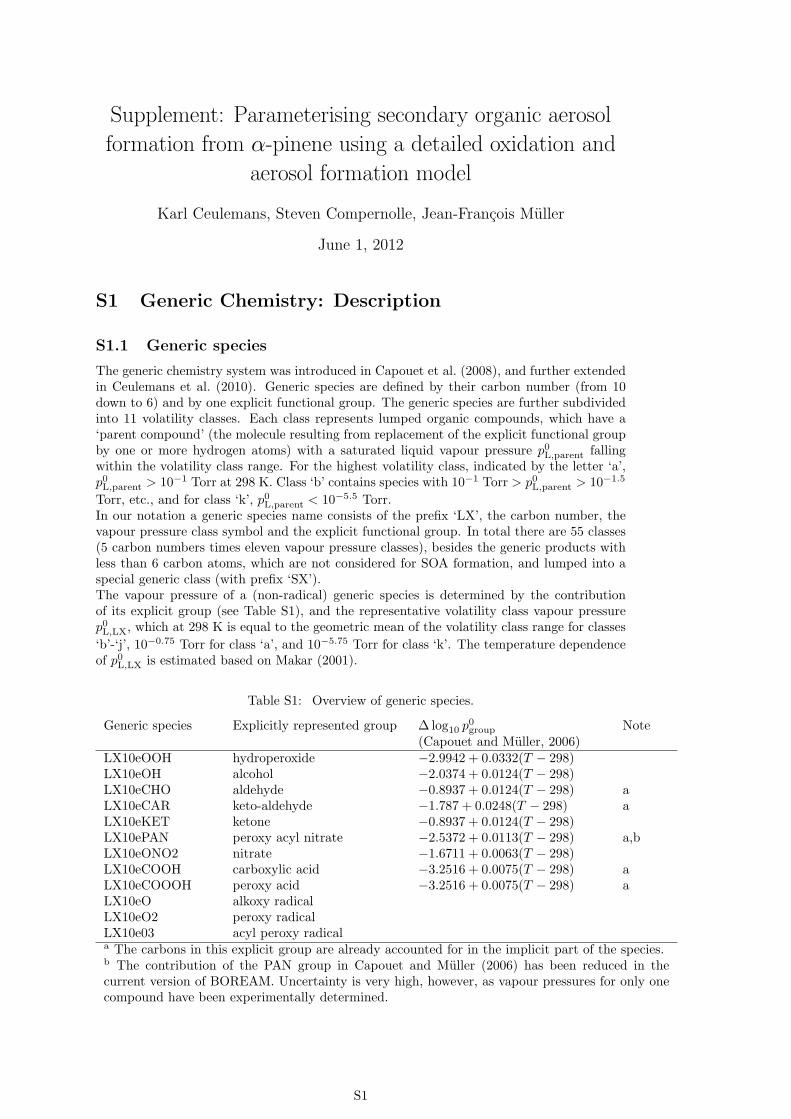
Supplement: Parameterising secondary organic aerosol formation from α-pinene using a detailed oxidation and aerosol formation model Karl Ceulemans, Steven Compernolle, Jean-Fran¸cois M¨ uller June 1, 2012 S1 Generic Chemistry: Description S1.1 Generic species The generic chemistry system was introduced in Capouet et al. (2008), and further extended in Ceulemans et al. (2010). Generic species are defined by their carbon number (from 10 down to 6) and by one explicit functional group. The generic species are further subdivided into 11 volatility classes. Each class represents lumped organic compounds, which have a ‘parent compound’ (the molecule resulting from replacement of the explicit functional group by one or more hydrogen atoms) with a saturated liquid vapour pressure p 0 L,parent falling within the volatility class range. For the highest volatility class, indicated by the letter ‘a’, p 0 L,parent > 10 -1 Torr at 298 K. Class ‘b’ contains species with 10 -1 Torr >p 0 L,parent > 10 -1.5 Torr, etc., and for class ‘k’, p 0 L,parent < 10 -5.5 Torr. In our notation a generic species name consists of the prefix ‘LX’, the carbon number, the vapour pressure class symbol and the explicit functional group. In total there are 55 classes (5 carbon numbers times eleven vapour pressure classes), besides the generic products with less than 6 carbon atoms, which are not considered for SOA formation, and lumped into a special generic class (with prefix ‘SX’). The vapour pressure of a (non-radical) generic species is determined by the contribution of its explicit group (see Table S1), and the representative volatility class vapour pressure p 0 L,LX , which at 298 K is equal to the geometric mean of the volatility class range for classes ‘b’-‘j’, 10 -0.75 Torr for class ‘a’, and 10 -5.75 Torr for class ‘k’. The temperature dependence of p 0 L,LX is estimated based on Makar (2001). Table S1: Overview of generic species. Generic species Explicitly represented group ∆ log 10 p 0 group Note (Capouet and M¨ uller, 2006) LX10eOOH hydroperoxide -2.9942 + 0.0332(T - 298) LX10eOH alcohol -2.0374 + 0.0124(T - 298) LX10eCHO aldehyde -0.8937 + 0.0124(T - 298) a LX10eCAR keto-aldehyde -1.787 + 0.0248(T - 298) a LX10eKET ketone -0.8937 + 0.0124(T - 298) LX10ePAN peroxy acyl nitrate -2.5372 + 0.0113(T - 298) a,b LX10eONO2 nitrate -1.6711 + 0.0063(T - 298) LX10eCOOH carboxylic acid -3.2516 + 0.0075(T - 298) a LX10eCOOOH peroxy acid -3.2516 + 0.0075(T - 298) a LX10eO alkoxy radical LX10eO2 peroxy radical LX10e03 acyl peroxy radical a The carbons in this explicit group are already accounted for in the implicit part of the species. b The contribution of the PAN group in Capouet and M¨ uller (2006) has been reduced in the current version of BOREAM. Uncertainty is very high, however, as vapour pressures for only one compound have been experimentally determined. S1
Transcript of Supplement: Parameterising secondary organic … alcohol 2:0374+0:0124(T 298) LX10eCHO aldehyde 0:...
Supplement: Parameterising secondary organic aerosol
formation from α-pinene using a detailed oxidation and
aerosol formation model
Karl Ceulemans, Steven Compernolle, Jean-Francois Muller
June 1, 2012
S1 Generic Chemistry: Description
S1.1 Generic species
The generic chemistry system was introduced in Capouet et al. (2008), and further extendedin Ceulemans et al. (2010). Generic species are defined by their carbon number (from 10down to 6) and by one explicit functional group. The generic species are further subdividedinto 11 volatility classes. Each class represents lumped organic compounds, which have a‘parent compound’ (the molecule resulting from replacement of the explicit functional groupby one or more hydrogen atoms) with a saturated liquid vapour pressure p0L,parent fallingwithin the volatility class range. For the highest volatility class, indicated by the letter ‘a’,p0L,parent > 10−1 Torr at 298 K. Class ‘b’ contains species with 10−1 Torr > p0L,parent > 10−1.5
Torr, etc., and for class ‘k’, p0L,parent < 10−5.5 Torr.In our notation a generic species name consists of the prefix ‘LX’, the carbon number, thevapour pressure class symbol and the explicit functional group. In total there are 55 classes(5 carbon numbers times eleven vapour pressure classes), besides the generic products withless than 6 carbon atoms, which are not considered for SOA formation, and lumped into aspecial generic class (with prefix ‘SX’).The vapour pressure of a (non-radical) generic species is determined by the contributionof its explicit group (see Table S1), and the representative volatility class vapour pressurep0L,LX, which at 298 K is equal to the geometric mean of the volatility class range for classes
‘b’-‘j’, 10−0.75 Torr for class ‘a’, and 10−5.75 Torr for class ‘k’. The temperature dependenceof p0L,LX is estimated based on Makar (2001).
Table S1: Overview of generic species.
Generic species Explicitly represented group ∆ log10 p0group Note
(Capouet and Muller, 2006)LX10eOOH hydroperoxide −2.9942 + 0.0332(T − 298)LX10eOH alcohol −2.0374 + 0.0124(T − 298)LX10eCHO aldehyde −0.8937 + 0.0124(T − 298) aLX10eCAR keto-aldehyde −1.787 + 0.0248(T − 298) aLX10eKET ketone −0.8937 + 0.0124(T − 298)LX10ePAN peroxy acyl nitrate −2.5372 + 0.0113(T − 298) a,bLX10eONO2 nitrate −1.6711 + 0.0063(T − 298)LX10eCOOH carboxylic acid −3.2516 + 0.0075(T − 298) aLX10eCOOOH peroxy acid −3.2516 + 0.0075(T − 298) aLX10eO alkoxy radicalLX10eO2 peroxy radicalLX10e03 acyl peroxy radicala The carbons in this explicit group are already accounted for in the implicit part of the species.b The contribution of the PAN group in Capouet and Muller (2006) has been reduced in thecurrent version of BOREAM. Uncertainty is very high, however, as vapour pressures for only onecompound have been experimentally determined.
S1
S1 GENERIC CHEMISTRY: DESCRIPTION S2
S1.2 Generic reactions
In the following tables, the reactions for one category of generic species are listed. Thereaction rates and products are based on the reaction rates and product distributions forsimilar explicit compounds.
S1 GENERIC CHEMISTRY: DESCRIPTION S3
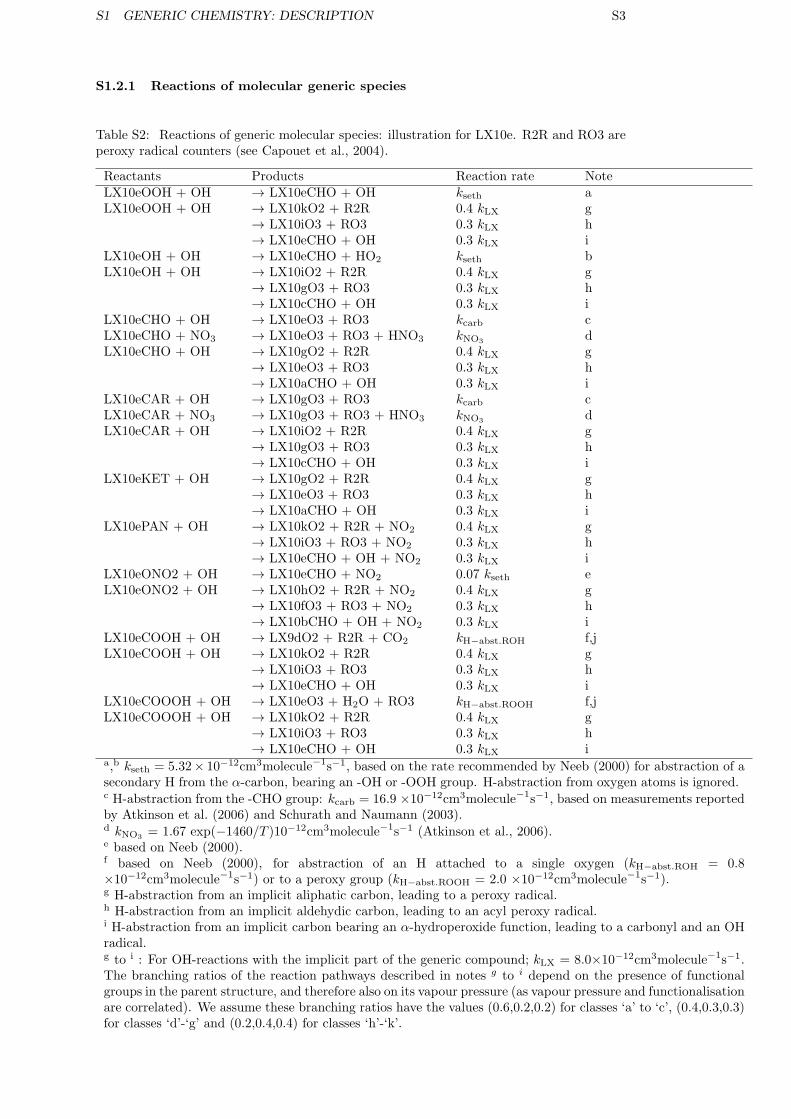
S1.2.1 Reactions of molecular generic species
Table S2: Reactions of generic molecular species: illustration for LX10e. R2R and RO3 areperoxy radical counters (see Capouet et al., 2004).
Reactants Products Reaction rate NoteLX10eOOH + OH → LX10eCHO + OH kseth aLX10eOOH + OH → LX10kO2 + R2R 0.4 kLX g
→ LX10iO3 + RO3 0.3 kLX h→ LX10eCHO + OH 0.3 kLX i
LX10eOH + OH → LX10eCHO + HO2 kseth bLX10eOH + OH → LX10iO2 + R2R 0.4 kLX g
→ LX10gO3 + RO3 0.3 kLX h→ LX10cCHO + OH 0.3 kLX i
LX10eCHO + OH → LX10eO3 + RO3 kcarb cLX10eCHO + NO3 → LX10eO3 + RO3 + HNO3 kNO3 dLX10eCHO + OH → LX10gO2 + R2R 0.4 kLX g
→ LX10eO3 + RO3 0.3 kLX h→ LX10aCHO + OH 0.3 kLX i
LX10eCAR + OH → LX10gO3 + RO3 kcarb cLX10eCAR + NO3 → LX10gO3 + RO3 + HNO3 kNO3 dLX10eCAR + OH → LX10iO2 + R2R 0.4 kLX g
→ LX10gO3 + RO3 0.3 kLX h→ LX10cCHO + OH 0.3 kLX i
LX10eKET + OH → LX10gO2 + R2R 0.4 kLX g→ LX10eO3 + RO3 0.3 kLX h→ LX10aCHO + OH 0.3 kLX i
LX10ePAN + OH → LX10kO2 + R2R + NO2 0.4 kLX g→ LX10iO3 + RO3 + NO2 0.3 kLX h→ LX10eCHO + OH + NO2 0.3 kLX i
LX10eONO2 + OH → LX10eCHO + NO2 0.07 kseth eLX10eONO2 + OH → LX10hO2 + R2R + NO2 0.4 kLX g
→ LX10fO3 + RO3 + NO2 0.3 kLX h→ LX10bCHO + OH + NO2 0.3 kLX i
LX10eCOOH + OH → LX9dO2 + R2R + CO2 kH−abst.ROH f,jLX10eCOOH + OH → LX10kO2 + R2R 0.4 kLX g
→ LX10iO3 + RO3 0.3 kLX h→ LX10eCHO + OH 0.3 kLX i
LX10eCOOOH + OH → LX10eO3 + H2O + RO3 kH−abst.ROOH f,jLX10eCOOOH + OH → LX10kO2 + R2R 0.4 kLX g
→ LX10iO3 + RO3 0.3 kLX h→ LX10eCHO + OH 0.3 kLX i
a,b kseth = 5.32× 10⁻¹²cm3molecule−1s−1, based on the rate recommended by Neeb (2000) for abstraction of asecondary H from the α-carbon, bearing an -OH or -OOH group. H-abstraction from oxygen atoms is ignored.c H-abstraction from the -CHO group: kcarb = 16.9 ×10⁻¹²cm3molecule−1s−1, based on measurements reportedby Atkinson et al. (2006) and Schurath and Naumann (2003).d kNO3 = 1.67 exp(−1460/T )10−12cm3molecule−1s−1 (Atkinson et al., 2006).e based on Neeb (2000).f based on Neeb (2000), for abstraction of an H attached to a single oxygen (kH−abst.ROH = 0.8×10⁻¹²cm3molecule−1s−1) or to a peroxy group (kH−abst.ROOH = 2.0 ×10⁻¹²cm3molecule−1s−1).g H-abstraction from an implicit aliphatic carbon, leading to a peroxy radical.h H-abstraction from an implicit aldehydic carbon, leading to an acyl peroxy radical.i H-abstraction from an implicit carbon bearing an α-hydroperoxide function, leading to a carbonyl and an OHradical.g to i : For OH-reactions with the implicit part of the generic compound; kLX = 8.0×10⁻¹²cm3molecule−1s−1.The branching ratios of the reaction pathways described in notes g to i depend on the presence of functionalgroups in the parent structure, and therefore also on its vapour pressure (as vapour pressure and functionalisationare correlated). We assume these branching ratios have the values (0.6,0.2,0.2) for classes ‘a’ to ‘c’, (0.4,0.3,0.3)for classes ‘d’-‘g’ and (0.2,0.4,0.4) for classes ‘h’-‘k’.
S1 GENERIC CHEMISTRY: DESCRIPTION S4
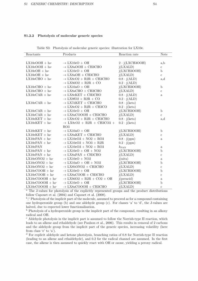
S1.2.2 Photolysis of molecular generic species
Table S3: Photolysis of molecular generic species: illustration for LX10e.
Reactants Products Reaction rate Note
LX10eOOH + hν → LX10eO + OH 2 · j(LXCH3OOH) a,bLX10eOOH + hν → LX8aOOH + CH3CHO j(LXALD) cLX10eOH + hν → LX10cO + OH j(LXCH3OOH) bLX10eOH + hν → LX8aOH + CH3CHO j(LXALD) cLX10eCHO + hν → LX8cO2 + R2R + CH3CHO 0.8 · j(ALD) a,d
→ LX9dO2 + R2R + CO 0.2 · j(ALD)LX10eCHO + hν → LX10aO + OH j(LXCH3OOH) bLX10eCHO + hν → LX8aCHO + CH3CHO j(LXALD) cLX10eCAR + hν → LX8eKET + CH3CHO 0.8 · j(ALD) a
→ LX9fO2 + R2R + CO 0.2 · j(ALD)LX10eCAR + hν → LX7dKET + CH3CHO 0.8 · j(keto)
→ LX8eO2 + R2R + CH3CO 0.2 · j(keto)LX10eCAR + hν → LX10cO + OH j(LXCH3OOH) bLX10eCAR + hν → LX8aCOOOH + CH3CHO j(LXALD) cLX10eKET + hν → LX8cO2 + R2R + CH3CHO 0.8 · j(keto) a,dLX10eKET + hν → LX8cO2 + R2R + CH3CO3 +
RO30.2 · j(keto)
LX10eKET + hν → LX10aO + OH j(LXCH3OOH) bLX10eKET + hν → LX8aKET + CH3CHO j(LXALD) cLX10ePAN + hν → LX10eO3 + NO2 + RO3 0.8 · j(ppn) aLX10ePAN + hν → LX10eO2 + NO3 + R2R 0.2 · j(ppn)LX10ePAN → LX10eO3 + NO2 + RO3 kPAN aLX10ePAN + hν → LX10eO + OH + NO2 j(LXCH3OOH) bLX10ePAN + hν → LX8aPAN + CH3CHO j(LXALD) cLX10eONO2 + hν → LX10eO + NO2 j(nitu) aLX10eONO2 + hν → LX10aO + OH + NO2 j(LXCH3OOH) bLX10eONO2 + hν → LX8bONO2 + CH3CHO j(LXALD) cLX10eCOOH + hν → LX10eO + OH j(LXCH3OOH) bLX10eCOOH + hν → LX8aCOOH + CH3CHO j(LXALD) cLX10eCOOOH + hν → LX9dO2 + R2R + CO2 + OH j(peracid) aLX10eCOOOH + hν → LX10eO + OH j(LXCH3OOH) bLX10eCOOOH + hν → LX8aCOOOH + CH3CHO j(LXALD) ca The J-values for photolysis of the explicitly represented groups and the product distributionsfollow Capouet et al. (2004) and Capouet et al. (2008).b,c Photolysis of the implicit part of the molecule, assumed to proceed as for a compound containingone hydroperoxide group (b) and one aldehyde group (c). For classes ‘a’ to ‘d’, the J-values arehalved, due to expected lower functionalisation.b Photolysis of a hydroperoxide group in the implicit part of the compound, resulting in an alkoxyradical and OH.c Aldehyde photolysis in the implicit part is assumed to follow the Norrish-type II reaction, whichleads to an alkene and ethaldehyde (see Paulson et al., 2006). This results in removal of 2 carbonsand the aldehyde group from the implicit part of the generic species, increasing volatility (herefrom class ‘e’ to ‘a’).d For explicit aldehyde and ketone photolysis, branching ratios of 0.8 for Norrish-type II reaction(leading to an alkene and ethaldehyde), and 0.2 for the radical channel are assumed. In the firstcase, the alkene is then assumed to quickly react with OH or ozone, yielding a peroxy radical.
S1 GENERIC CHEMISTRY: DESCRIPTION S5
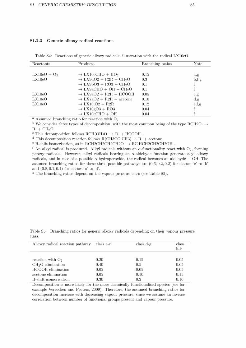
S1.2.3 Generic alkoxy radical reactions
Table S4: Reactions of generic alkoxy radicals: illustration with the radical LX10eO.
Reactants Products Branching ratios Note
LX10eO + O2 → LX10eCHO + HO2 0.15 a,gLX10eO → LX9dO2 + R2R + CH2O 0.3 b,f,g
→ LX9bO3 + RO3 + CH2O 0.1 f→ LX9aCHO + OH + CH2O 0.1 f
LX10eO → LX9aO2 + R2R + HCOOH 0.05 c,gLX10eO → LX7aO2 + R2R + acetone 0.10 d,gLX10eO → LX10iO2 + R2R 0.12 e,f,g
→ LX10gO3 + RO3 0.04 f→ LX10cCHO + OH 0.04 f
a Assumed branching ratio for reaction with O2.b We consider three types of decomposition, with the most common being of the type RCH2O· →R· + CH2O.c This decomposition follows RCH(OH)O· → R· + HCOOH .d This decomposition reaction follows R(CH3CO·CH3) → R· + acetone .e H-shift isomerisation, as in RCH2CH2CH2CH2O· → RC·HCH2CH2CH2OH .f An alkyl radical is produced. Alkyl radicals without an α-functionality react with O2, formingperoxy radicals. However, alkyl radicals bearing an α-aldehyde function generate acyl alkoxyradicals, and in case of a possible α-hydroperoxide, the radical becomes an aldehyde + OH. Theassumed branching ratios for these three possible pathways are (0.6, 0.2, 0.2) for classes ‘e’ to ‘k’and (0.8, 0.1, 0.1) for classes ‘a’ to ‘d’.g The branching ratios depend on the vapour pressure class (see Table S5).
Table S5: Branching ratios for generic alkoxy radicals depending on their vapour pressureclass.
Alkoxy radical reaction pathway class a-c class d-g classh-k
reaction with O2 0.20 0.15 0.05CH2O elimination 0.40 0.5 0.65HCOOH elimination 0.05 0.05 0.05acetone elimination 0.05 0.10 0.15H-shift isomerisation 0.30 0.2 0.10Decomposition is more likely for the more chemically functionalised species (see forexample Vereecken and Peeters, 2009). Therefore, the assumed branching ratios fordecomposition increase with decreasing vapour pressure, since we assume an inversecorrelation between number of functional groups present and vapour pressure.
S1 GENERIC CHEMISTRY: DESCRIPTION S6
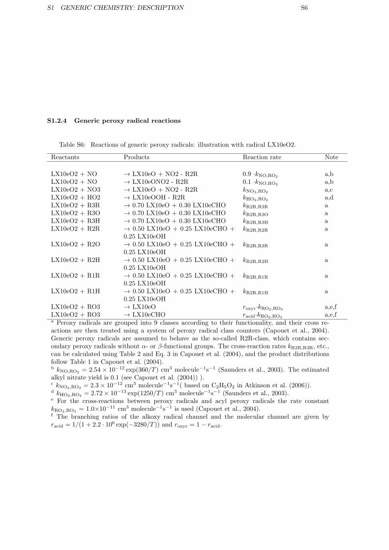
S1.2.4 Generic peroxy radical reactions
Table S6: Reactions of generic peroxy radicals: illustration with radical LX10eO2.
Reactants Products Reaction rate Note
LX10eO2 + NO → LX10eO + NO2 - R2R 0.9 ·kNO,RO2 a,bLX10eO2 + NO → LX10eONO2 - R2R 0.1 ·kNO,RO2 a,bLX10eO2 + NO3 → LX10eO + NO2 - R2R kNO3,RO2 a,cLX10eO2 + HO2 → LX10eOOH - R2R kHO2,RO2 a,dLX10eO2 + R3R → 0.70 LX10eO + 0.30 LX10eCHO kR2R,R3R aLX10eO2 + R3O → 0.70 LX10eO + 0.30 LX10eCHO kR2R,R3O aLX10eO2 + R3H → 0.70 LX10eO + 0.30 LX10eCHO kR2R,R3H aLX10eO2 + R2R → 0.50 LX10eO + 0.25 LX10eCHO +
0.25 LX10eOHkR2R,R2R a
LX10eO2 + R2O → 0.50 LX10eO + 0.25 LX10eCHO +0.25 LX10eOH
kR2R,R3R a
LX10eO2 + R2H → 0.50 LX10eO + 0.25 LX10eCHO +0.25 LX10eOH
kR2R,R2H a
LX10eO2 + R1R → 0.50 LX10eO + 0.25 LX10eCHO +0.25 LX10eOH
kR2R,R1R a
LX10eO2 + R1H → 0.50 LX10eO + 0.25 LX10eCHO +0.25 LX10eOH
kR2R,R1H a
LX10eO2 + RO3 → LX10eO roxyr·kRO2,RO3 a,e,fLX10eO2 + RO3 → LX10eCHO racid·kRO2,RO3 a,e,fa Peroxy radicals are grouped into 9 classes according to their functionality, and their cross re-actions are then treated using a system of peroxy radical class counters (Capouet et al., 2004).Generic peroxy radicals are assumed to behave as the so-called R2R-class, which contains sec-ondary peroxy radicals without α- or β-functional groups. The cross-reaction rates kR2R,R3R, etc.,can be calculated using Table 2 and Eq. 3 in Capouet et al. (2004), and the product distributionsfollow Table 1 in Capouet et al. (2004).b kNO,RO2 = 2.54 × 10⁻¹² exp(360/T ) cm3 molecule−1s−1 (Saunders et al., 2003). The estimatedalkyl nitrate yield is 0.1 (see Capouet et al. (2004)) ).c kNO3,RO2 = 2.3× 10⁻¹² cm3 molecule−1s−1( based on C2H5O2 in Atkinson et al. (2006)).d kHO2,RO2 = 2.72× 10⁻¹³ exp(1250/T ) cm3 molecule−1s−1 (Saunders et al., 2003).e For the cross-reactions between peroxy radicals and acyl peroxy radicals the rate constantkRO2,RO3 = 1.0×10⁻¹¹ cm3 molecule−1s−1 is used (Capouet et al., 2004).f The branching ratios of the alkoxy radical channel and the molecular channel are given byracid = 1/(1 + 2.2 · 106 exp(−3280/T )) and roxyr = 1− racid.
S1 GENERIC CHEMISTRY: DESCRIPTION S7
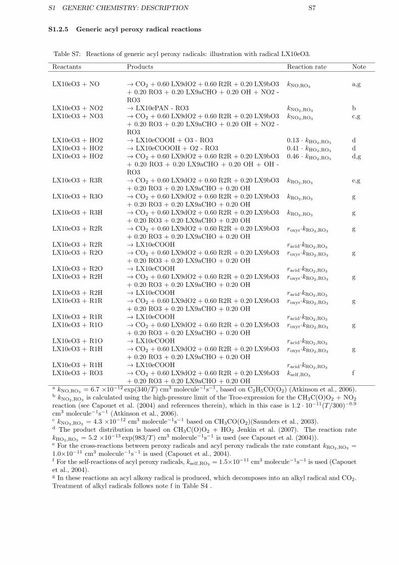
S1.2.5 Generic acyl peroxy radical reactions
Table S7: Reactions of generic acyl peroxy radicals: illustration with radical LX10eO3.
Reactants Products Reaction rate Note
LX10eO3 + NO → CO2 + 0.60 LX9dO2 + 0.60 R2R + 0.20 LX9bO3+ 0.20 RO3 + 0.20 LX9aCHO + 0.20 OH + NO2 -RO3
kNO,RO3 a,g
LX10eO3 + NO2 → LX10ePAN - RO3 kNO2,RO3 bLX10eO3 + NO3 → CO2 + 0.60 LX9dO2 + 0.60 R2R + 0.20 LX9bO3
+ 0.20 RO3 + 0.20 LX9aCHO + 0.20 OH + NO2 -RO3
kNO3,RO3 c,g
LX10eO3 + HO2 → LX10eCOOH + O3 - RO3 0.13 · kHO2,RO3 dLX10eO3 + HO2 → LX10eCOOOH + O2 - RO3 0.41 · kHO2,RO3 dLX10eO3 + HO2 → CO2 + 0.60 LX9dO2 + 0.60 R2R + 0.20 LX9bO3
+ 0.20 RO3 + 0.20 LX9aCHO + 0.20 OH + OH -RO3
0.46 · kHO2,RO3 d,g
LX10eO3 + R3R → CO2 + 0.60 LX9dO2 + 0.60 R2R + 0.20 LX9bO3+ 0.20 RO3 + 0.20 LX9aCHO + 0.20 OH
kRO2,RO3 e,g
LX10eO3 + R3O → CO2 + 0.60 LX9dO2 + 0.60 R2R + 0.20 LX9bO3+ 0.20 RO3 + 0.20 LX9aCHO + 0.20 OH
kRO2,RO3 g
LX10eO3 + R3H → CO2 + 0.60 LX9dO2 + 0.60 R2R + 0.20 LX9bO3+ 0.20 RO3 + 0.20 LX9aCHO + 0.20 OH
kRO2,RO3 g
LX10eO3 + R2R → CO2 + 0.60 LX9dO2 + 0.60 R2R + 0.20 LX9bO3+ 0.20 RO3 + 0.20 LX9aCHO + 0.20 OH
roxyr·kRO2,RO3 g
LX10eO3 + R2R → LX10eCOOH racid·kRO2,RO3
LX10eO3 + R2O → CO2 + 0.60 LX9dO2 + 0.60 R2R + 0.20 LX9bO3+ 0.20 RO3 + 0.20 LX9aCHO + 0.20 OH
roxyr·kRO2,RO3 g
LX10eO3 + R2O → LX10eCOOH racid·kRO2,RO3
LX10eO3 + R2H → CO2 + 0.60 LX9dO2 + 0.60 R2R + 0.20 LX9bO3+ 0.20 RO3 + 0.20 LX9aCHO + 0.20 OH
roxyr·kRO2,RO3g
LX10eO3 + R2H → LX10eCOOH racid·kRO2,RO3
LX10eO3 + R1R → CO2 + 0.60 LX9dO2 + 0.60 R2R + 0.20 LX9bO3+ 0.20 RO3 + 0.20 LX9aCHO + 0.20 OH
roxyr·kRO2,RO3 g
LX10eO3 + R1R → LX10eCOOH racid·kRO2,RO3
LX10eO3 + R1O → CO2 + 0.60 LX9dO2 + 0.60 R2R + 0.20 LX9bO3+ 0.20 RO3 + 0.20 LX9aCHO + 0.20 OH
roxyr·kRO2,RO3 g
LX10eO3 + R1O → LX10eCOOH racid·kRO2,RO3
LX10eO3 + R1H → CO2 + 0.60 LX9dO2 + 0.60 R2R + 0.20 LX9bO3+ 0.20 RO3 + 0.20 LX9aCHO + 0.20 OH
roxyr·kRO2,RO3 g
LX10eO3 + R1H → LX10eCOOH racid·kRO2,RO3
LX10eO3 + RO3 → CO2 + 0.60 LX9dO2 + 0.60 R2R + 0.20 LX9bO3+ 0.20 RO3 + 0.20 LX9aCHO + 0.20 OH
kself,RO3 f
a kNO,RO3 = 6.7 ×10⁻¹² exp(340/T ) cm3 molecule−1s−1, based on C2H5CO(O2) (Atkinson et al., 2006).b kNO2,RO3 is calculated using the high-pressure limit of the Troe-expression for the CH3C(O)O2 + NO2
reaction (see Capouet et al. (2004) and references therein), which in this case is 1.2 · 10−11(T/300)−0.9
cm3 molecule−1s−1 (Atkinson et al., 2006).c kNO3,RO3 = 4.3 ×10⁻¹² cm3 molecule−1s−1 based on CH3CO(O2)(Saunders et al., 2003).d The product distribution is based on CH3C(O)O2 + HO2 Jenkin et al. (2007). The reaction ratekHO2,RO3 = 5.2 ×10⁻¹³ exp(983/T ) cm3 molecule−1s−1 is used (see Capouet et al. (2004)).e For the cross-reactions between peroxy radicals and acyl peroxy radicals the rate constant kRO2,RO3 =1.0×10⁻¹¹ cm3 molecule−1s−1 is used (Capouet et al., 2004).f For the self-reactions of acyl peroxy radicals, kself,RO3 = 1.5×10⁻¹¹ cm3 molecule−1s−1 is used (Capouetet al., 2004).g In these reactions an acyl alkoxy radical is produced, which decomposes into an alkyl radical and CO2.Treatment of alkyl radicals follows note f in Table S4 .
S2 BOREAM MODEL VALIDATION S8
S2 BOREAM Model validation
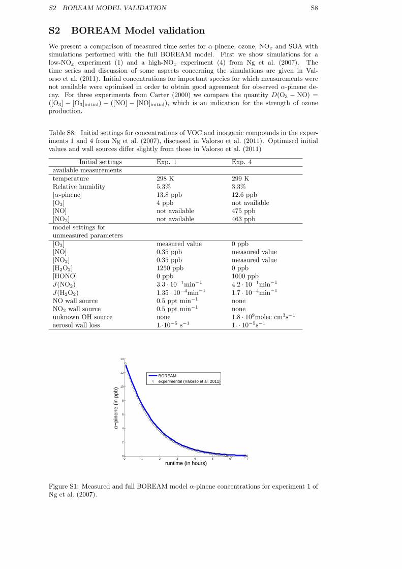
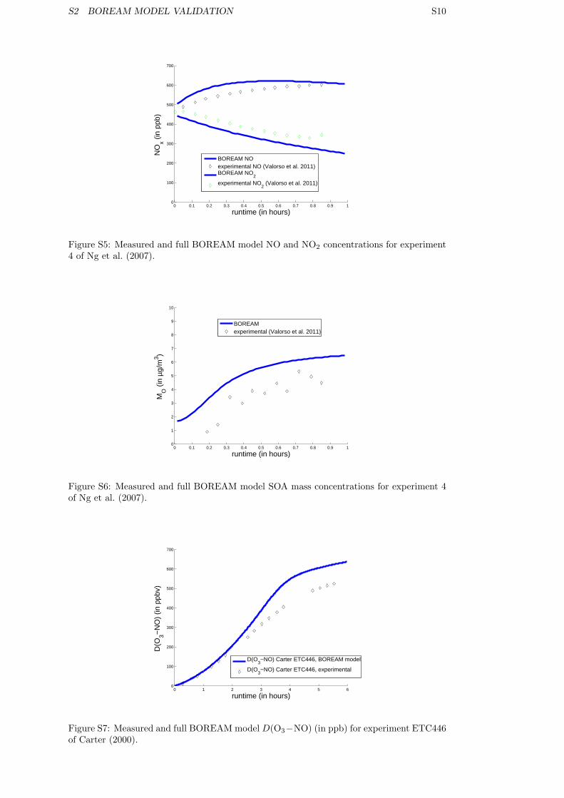
We present a comparison of measured time series for α-pinene, ozone, NOx and SOA withsimulations performed with the full BOREAM model. First we show simulations for alow-NOx experiment (1) and a high-NOx experiment (4) from Ng et al. (2007). Thetime series and discussion of some aspects concerning the simulations are given in Val-orso et al. (2011). Initial concentrations for important species for which measurements werenot available were optimised in order to obtain good agreement for observed α-pinene de-cay. For three experiments from Carter (2000) we compare the quantity D(O3 − NO) =([O3] − [O3]initial) − ([NO] − [NO]initial), which is an indication for the strength of ozoneproduction.
Table S8: Initial settings for concentrations of VOC and inorganic compounds in the exper-iments 1 and 4 from Ng et al. (2007), discussed in Valorso et al. (2011). Optimised initialvalues and wall sources differ slightly from those in Valorso et al. (2011)
Initial settings Exp. 1 Exp. 4available measurementstemperature 298 K 299 KRelative humidity 5.3% 3.3%[α-pinene] 13.8 ppb 12.6 ppb[O3] 4 ppb not available[NO] not available 475 ppb[NO2] not available 463 ppbmodel settings forunmeasured parameters[O3] measured value 0 ppb[NO] 0.35 ppb measured value[NO2] 0.35 ppb measured value[H2O2] 1250 ppb 0 ppb[HONO] 0 ppb 1000 ppbJ(NO2) 3.3 · 10−1min−1 4.2 · 10−1min−1
J(H2O2) 1.35 · 10−4min−1 1.7 · 10−4min−1
NO wall source 0.5 ppt min−1 noneNO2 wall source 0.5 ppt min−1 noneunknown OH source none 1.8 · 109molec cm3s−1
aerosol wall loss 1.·10−5 s−1 1. · 10−5s−1
0 1 2 3 4 5 6 70
2
4
6
8
10
12
14
runtime (in hours)
α−pi
nene
(in
ppb
)
BOREAMexperimental (Valorso et al. 2011)
Figure S1: Measured and full BOREAM model α-pinene concentrations for experiment 1 ofNg et al. (2007).
S2 BOREAM MODEL VALIDATION S9
0 1 2 3 4 5 6 70
5
10
15
20
25
30
35
40
runtime (in hours)
ozon
e (in
ppb
)
BOREAMexperimental (Valorso et al. 2011)
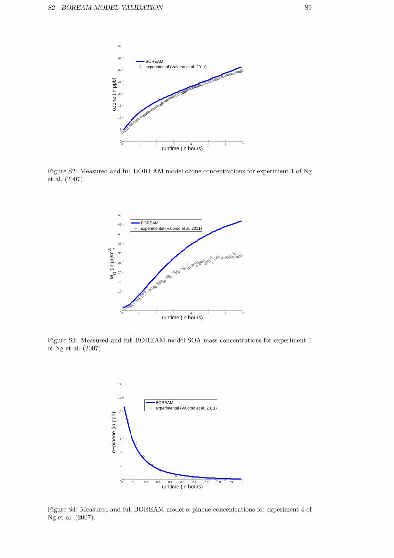
Figure S2: Measured and full BOREAM model ozone concentrations for experiment 1 of Nget al. (2007).
0 1 2 3 4 5 6 70
5
10
15
20
25
30
35
40
45
50
runtime (in hours)
MO
(in
µg/
m3 )
BOREAMexperimental (Valorso et al. 2011)
Figure S3: Measured and full BOREAM model SOA mass concentrations for experiment 1of Ng et al. (2007).
0 0.1 0.2 0.3 0.4 0.5 0.6 0.7 0.8 0.9 10
2
4
6
8
10
12
14
runtime (in hours)
α−pi
nene
(in
ppb
)
BOREAMexperimental (Valorso et al. 2011)
Figure S4: Measured and full BOREAM model α-pinene concentrations for experiment 4 ofNg et al. (2007).
S2 BOREAM MODEL VALIDATION S10
0 0.1 0.2 0.3 0.4 0.5 0.6 0.7 0.8 0.9 10
100
200
300
400
500
600
700
runtime (in hours)
NO
x (in
ppb
)
BOREAM NOexperimental NO (Valorso et al. 2011)BOREAM NO
2
experimental NO2 (Valorso et al. 2011)
Figure S5: Measured and full BOREAM model NO and NO2 concentrations for experiment4 of Ng et al. (2007).
0 0.1 0.2 0.3 0.4 0.5 0.6 0.7 0.8 0.9 10
1
2
3
4
5
6
7
8
9
10
runtime (in hours)
MO
(in
µg/
m3 )
BOREAMexperimental (Valorso et al. 2011)
Figure S6: Measured and full BOREAM model SOA mass concentrations for experiment 4of Ng et al. (2007).
0 1 2 3 4 5 60
100
200
300
400
500
600
700
runtime (in hours)
D(O
3−N
O)
(in p
pbv)
D(O3−NO) Carter ETC446, BOREAM model
D(O3−NO) Carter ETC446, experimental
Figure S7: Measured and full BOREAM model D(O3−NO) (in ppb) for experiment ETC446of Carter (2000).
S3 FITTING PROCEDURE FOR THE PHOTOCHEMICAL SOA LOSS S11
0 1 2 3 4 5 60
50
100
150
200
250
300
350
400
450
500
runtime (in hours)
D(O
3−N
O)
(in p
pbv)
D(O3−NO) Carter ETC447, BOREAM model
D(O3−NO) Carter ETC447, experimental
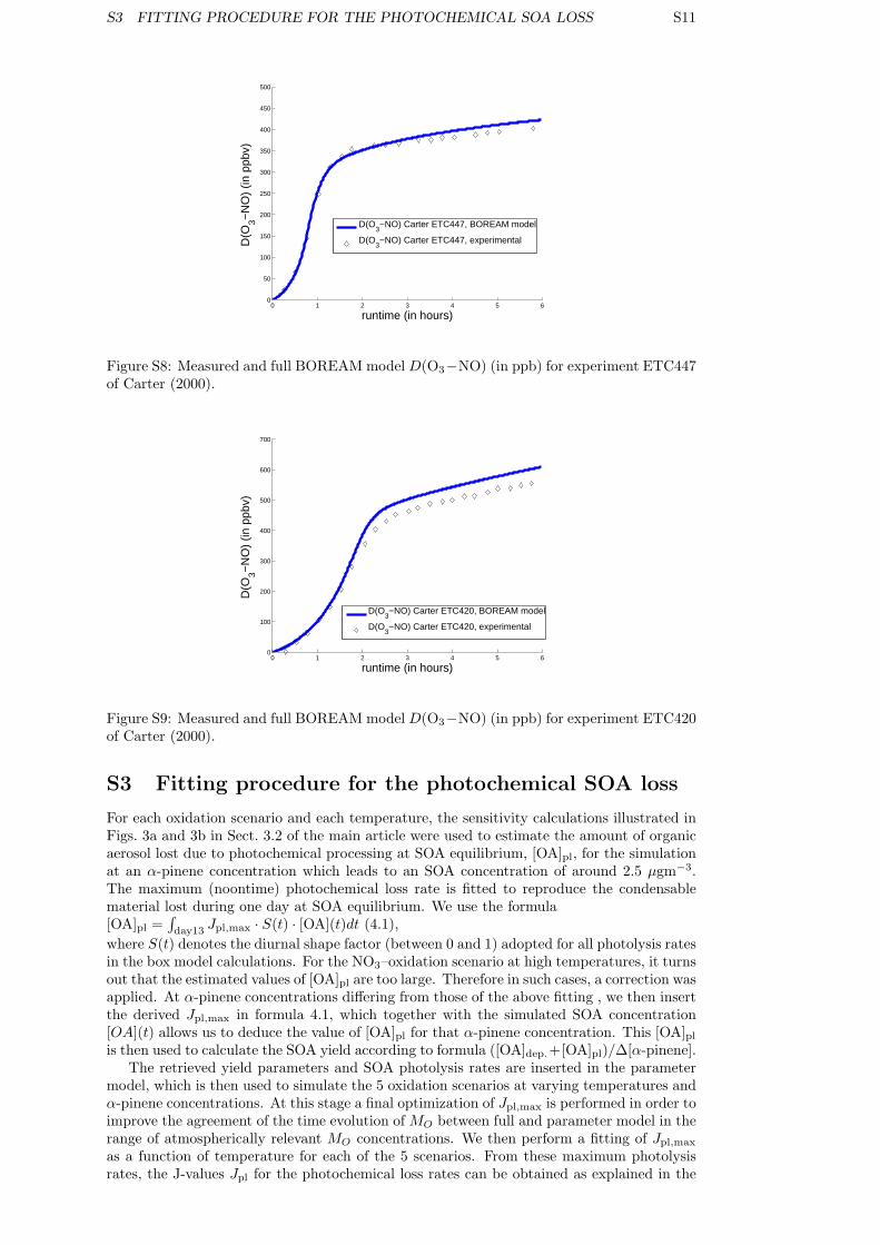
Figure S8: Measured and full BOREAM model D(O3−NO) (in ppb) for experiment ETC447of Carter (2000).
0 1 2 3 4 5 60
100
200
300
400
500
600
700
runtime (in hours)
D(O
3−N
O)
(in p
pbv)
D(O3−NO) Carter ETC420, BOREAM model
D(O3−NO) Carter ETC420, experimental
Figure S9: Measured and full BOREAM model D(O3−NO) (in ppb) for experiment ETC420of Carter (2000).
S3 Fitting procedure for the photochemical SOA loss
For each oxidation scenario and each temperature, the sensitivity calculations illustrated inFigs. 3a and 3b in Sect. 3.2 of the main article were used to estimate the amount of organicaerosol lost due to photochemical processing at SOA equilibrium, [OA]pl, for the simulationat an α-pinene concentration which leads to an SOA concentration of around 2.5 µgm−3.The maximum (noontime) photochemical loss rate is fitted to reproduce the condensablematerial lost during one day at SOA equilibrium. We use the formula[OA]pl =
∫day13
Jpl,max · S(t) · [OA](t)dt (4.1),
where S(t) denotes the diurnal shape factor (between 0 and 1) adopted for all photolysis ratesin the box model calculations. For the NO3–oxidation scenario at high temperatures, it turnsout that the estimated values of [OA]pl are too large. Therefore in such cases, a correction wasapplied. At α-pinene concentrations differing from those of the above fitting , we then insertthe derived Jpl,max in formula 4.1, which together with the simulated SOA concentration[OA](t) allows us to deduce the value of [OA]pl for that α-pinene concentration. This [OA]plis then used to calculate the SOA yield according to formula ([OA]dep.+[OA]pl)/∆[α-pinene].
The retrieved yield parameters and SOA photolysis rates are inserted in the parametermodel, which is then used to simulate the 5 oxidation scenarios at varying temperatures andα-pinene concentrations. At this stage a final optimization of Jpl,max is performed in order toimprove the agreement of the time evolution of MO between full and parameter model in therange of atmospherically relevant MO concentrations. We then perform a fitting of Jpl,max
as a function of temperature for each of the 5 scenarios. From these maximum photolysisrates, the J-values Jpl for the photochemical loss rates can be obtained as explained in the
S3 FITTING PROCEDURE FOR THE PHOTOCHEMICAL SOA LOSS S12
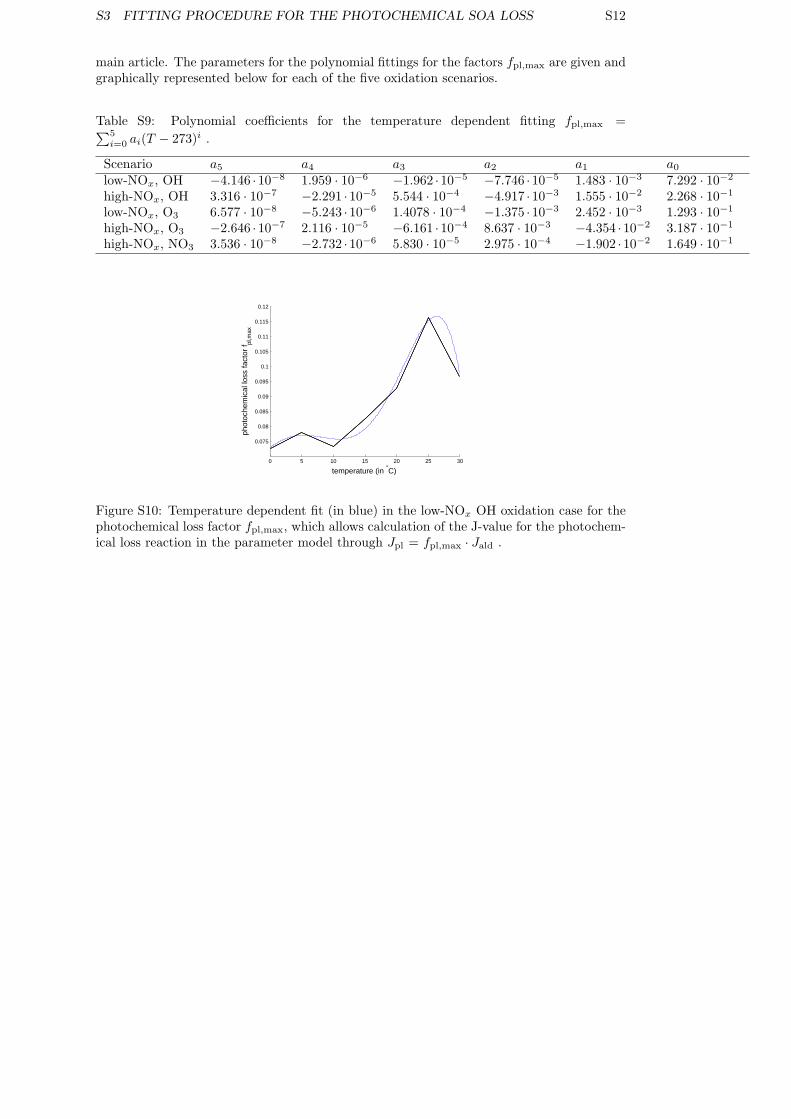
main article. The parameters for the polynomial fittings for the factors fpl,max are given andgraphically represented below for each of the five oxidation scenarios.
Table S9: Polynomial coefficients for the temperature dependent fitting fpl,max =∑5i=0 ai(T − 273)i .
Scenario a5 a4 a3 a2 a1 a0low-NOx, OH −4.146 ·10−8 1.959 · 10−6 −1.962 ·10−5 −7.746 ·10−5 1.483 · 10−3 7.292 · 10−2
high-NOx, OH 3.316 · 10−7 −2.291 ·10−5 5.544 · 10−4 −4.917 ·10−3 1.555 · 10−2 2.268 · 10−1
low-NOx, O3 6.577 · 10−8 −5.243 ·10−6 1.4078 · 10−4 −1.375 ·10−3 2.452 · 10−3 1.293 · 10−1
high-NOx, O3 −2.646 ·10−7 2.116 · 10−5 −6.161 ·10−4 8.637 · 10−3 −4.354 ·10−2 3.187 · 10−1
high-NOx, NO3 3.536 · 10−8 −2.732 ·10−6 5.830 · 10−5 2.975 · 10−4 −1.902 ·10−2 1.649 · 10−1
0 5 10 15 20 25 30
0.075
0.08
0.085
0.09
0.095
0.1
0.105
0.11
0.115
0.12
temperature (in °C)
phot
oche
mic
al lo
ss fa
ctor
f pl,m
ax
Figure S10: Temperature dependent fit (in blue) in the low-NOx OH oxidation case for thephotochemical loss factor fpl,max, which allows calculation of the J-value for the photochem-ical loss reaction in the parameter model through Jpl = fpl,max · Jald .
S3 FITTING PROCEDURE FOR THE PHOTOCHEMICAL SOA LOSS S13
0 5 10 15 20 25 300.2
0.3
0.4
0.5
0.6
0.7
0.8
0.9
temperature (in °C)
phot
oche
mic
al lo
ss fa
ctor
f pl,m
ax
0 5 10 15 20 25 300.105
0.11
0.115
0.12
0.125
0.13
0.135
0.14
0.145
temperature (in °C)
phot
oche
mic
al lo
ss fa
ctor
f pl,m
ax
0 5 10 15 20 25 300.2
0.3
0.4
0.5
0.6
0.7
0.8
0.9
1
temperature (in °C)
phot
oche
mic
al lo
ss fa
ctor
f pl,m
ax
0 5 10 15 20 25 300.02
0.04
0.06
0.08
0.1
0.12
0.14
0.16
0.18
temperature (in °C)
phot
oche
mic
al lo
ss fa
ctor
f pl,m
ax
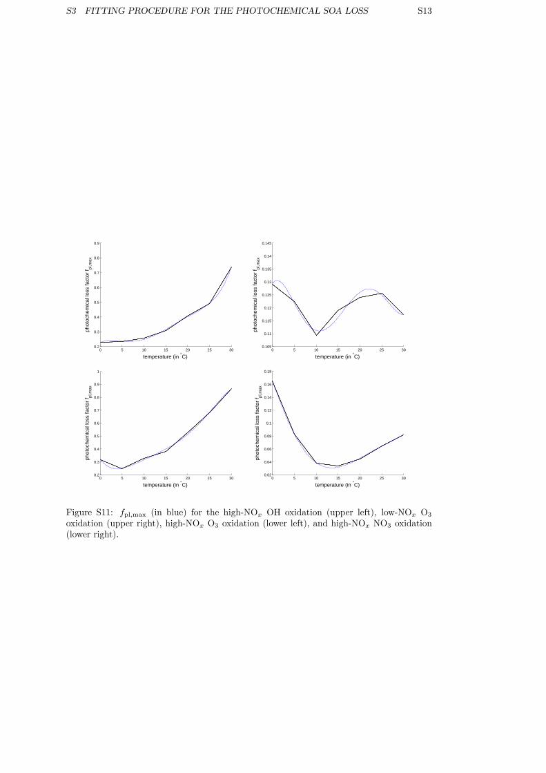
Figure S11: fpl,max (in blue) for the high-NOx OH oxidation (upper left), low-NOx O3
oxidation (upper right), high-NOx O3 oxidation (lower left), and high-NOx NO3 oxidation(lower right).
S4 SOA PARAMETERISATION AGREEMENT WITH FULL MODEL S14
S4 SOA parameterisation agreement with full model
In the following Table we evaluate the level of agreement between the full and the parametermodel for the 5 oxidation scenarios, which were simulated at 7 temperatures and at a numberof different α-pinene concentrations. In each simulation SOA build-up was simulated over 14day. Simulations for which the maximum MO reached did not fall in the range 0.5–20 µgm−3
were not considered. The following table provides the percentage of simulated days satisfyinga given level of agreement, using a deviation factor defined as exp(| log(MO,p/MO,f )|).
Table S10: Percentage of days for which the model deviation factor falls within the range 1to 1.25 (first part), or exceeds a factor 2 (second part).
Scenario 273 K 278 K 283 K 288 K 293 K 298 K 303 Klow-NOx, OH 98.2 97.3 94.6 91.7 85.7 84.5 81.2high-NOx, OH 95.5 95.0 93.5 87.9 80.1 89.3 78.6low-NOx, O3 98.2 98.2 97.6 91.1 83.3 76.8 80.4high-NOx, O3 92.9 83.6 94.4 92.1 88.9 85.7 57.1high-NOx, NO3 86.7 80.4 73.5 70.4 64.3 68.4 53.1low-NOx, OH 0 0 0 0 0 1.8 5.8high-NOx, OH 0 0 0.6 2.9 5.6 5.4 16.3low-NOx, O3 0 0 0 0 0 1.2 3.6high-NOx, O3 2.1 2.1 0 0.8 3.2 6.1 7.1high-NOx, NO3 3.1 2.7 2.0 1.0 5.1 11.2 27.6
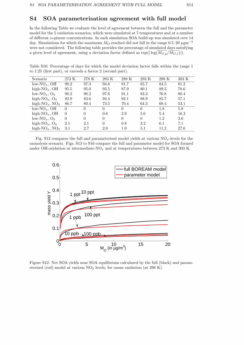
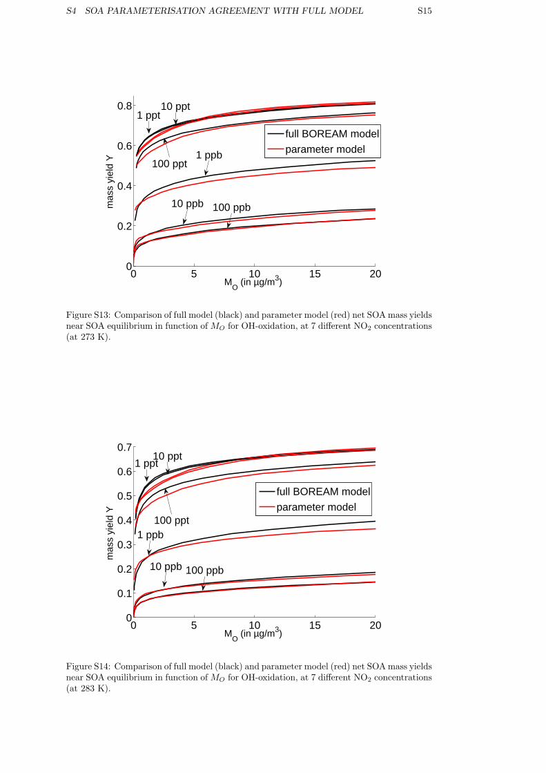
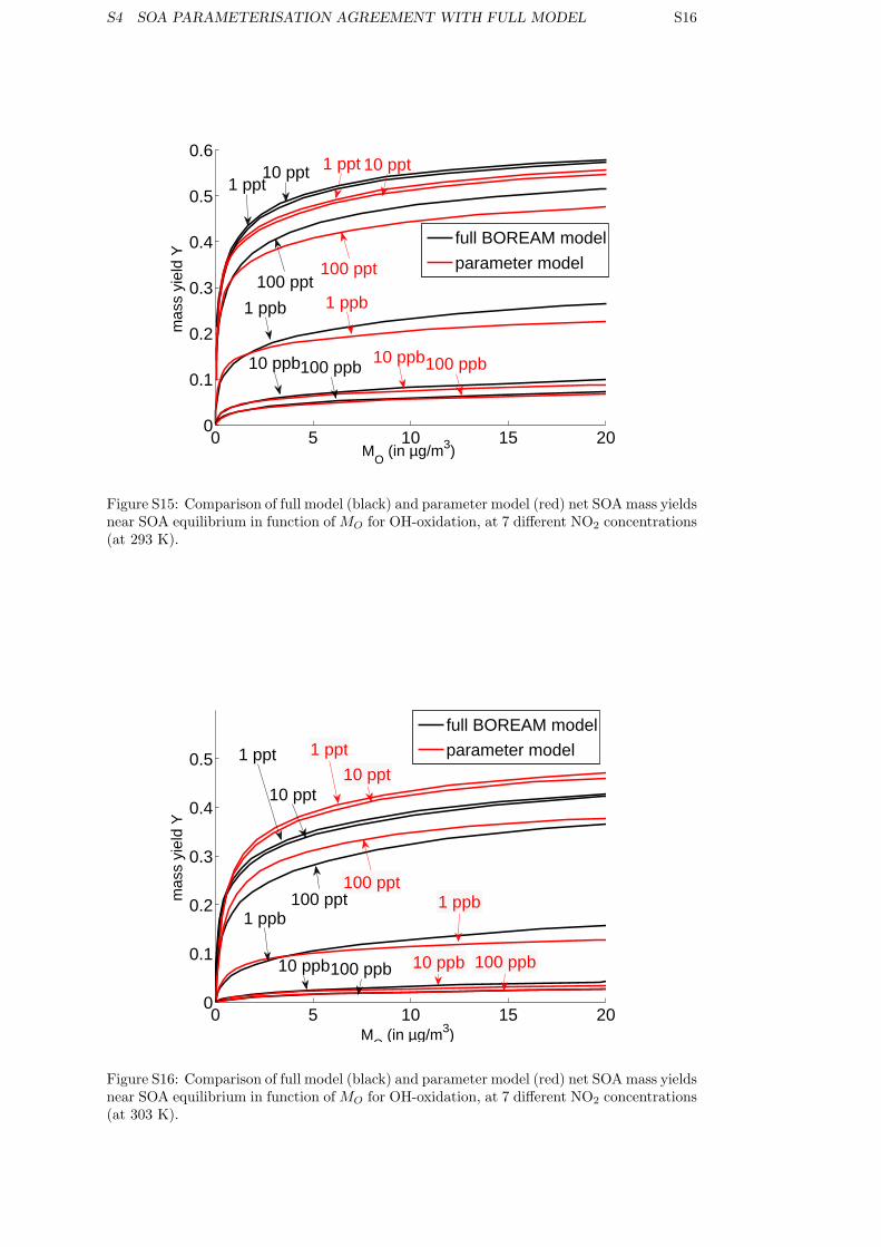
Fig. S12 compares the full and parameterised model yields at various NOx-levels for theozonolysis scenario. Figs. S13 to S16 compare the full and parameter model for SOA formedunder OH-oxidation at intermediate-NOx and at temperatures between 273 K and 303 K.
0 5 10 15 200
0.1
0.2
0.3
0.4
0.5
0.6
MO
(in µg/m3)
mas
s yi
eld
Y
full BOREAM modelparameter model
10 ppb
100 ppt
10 ppt
1 ppb
100 ppb
1 ppt
Figure S12: Net SOA yields near SOA equilibrium calculated by the full (black) and param-eterised (red) model at various NO2 levels, for ozone oxidation (at 298 K).
S4 SOA PARAMETERISATION AGREEMENT WITH FULL MODEL S15
0 5 10 15 200
0.2
0.4
0.6
0.8
MO
(in µg/m3)
mas
s yi
eld
Y
full BOREAM model
parameter model
1 ppt10 ppt
100 ppt1 ppb
10 ppb 100 ppb
Figure S13: Comparison of full model (black) and parameter model (red) net SOAmass yieldsnear SOA equilibrium in function of MO for OH-oxidation, at 7 different NO2 concentrations(at 273 K).
0 5 10 15 200
0.1
0.2
0.3
0.4
0.5
0.6
0.7
MO
(in µg/m3)
mas
s yi
eld
Y
full BOREAM model
parameter model
1 ppt10 ppt
100 ppt1 ppb
10 ppb 100 ppb
Figure S14: Comparison of full model (black) and parameter model (red) net SOAmass yieldsnear SOA equilibrium in function of MO for OH-oxidation, at 7 different NO2 concentrations(at 283 K).
S4 SOA PARAMETERISATION AGREEMENT WITH FULL MODEL S16
0 5 10 15 200
0.1
0.2
0.3
0.4
0.5
0.6
MO
(in µg/m3)
mas
s yi
eld
Y
full BOREAM model
parameter model
1 ppt10 ppt
10 ppb100 ppb 100 ppb10 ppb
1 ppb 1 ppb100 ppt
100 ppt
10 ppt1 ppt
Figure S15: Comparison of full model (black) and parameter model (red) net SOAmass yieldsnear SOA equilibrium in function of MO for OH-oxidation, at 7 different NO2 concentrations(at 293 K).
0 5 10 15 200
0.1
0.2
0.3
0.4
0.5
MO
(in µg/m3)
mas
s yi
eld
Y
full BOREAM model
parameter model
10 ppt
1 ppb
10 ppb100 ppb
1 ppt 1 ppt
10 ppt
10 ppb 100 ppb
1 ppb100 ppt100 ppt
Figure S16: Comparison of full model (black) and parameter model (red) net SOAmass yieldsnear SOA equilibrium in function of MO for OH-oxidation, at 7 different NO2 concentrations(at 303 K).
S5 FULL BOREAMAND PARAMETERMODEL FORAMBIENT CONDITIONS BASEDON IMAGESV2S17
S5 Full BOREAM and parameter model for ambientconditions based on IMAGESv2
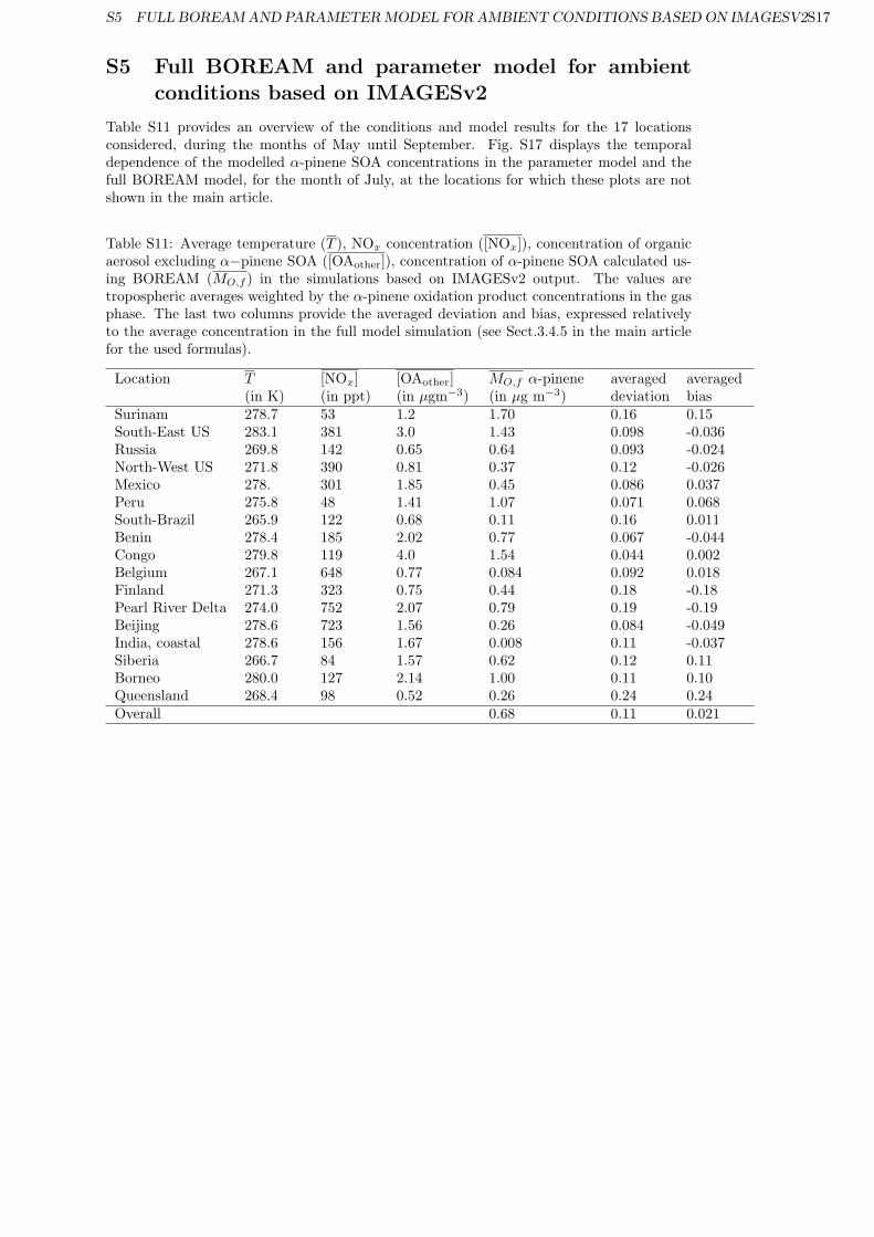
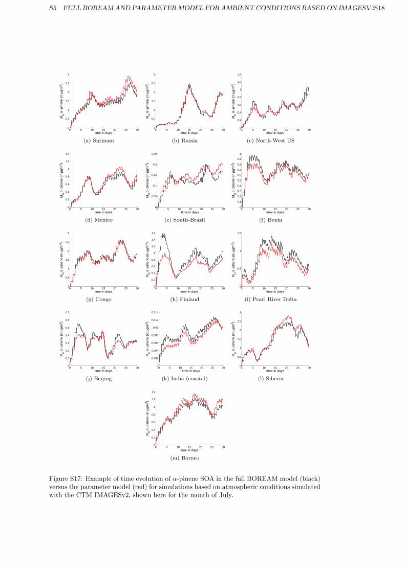
Table S11 provides an overview of the conditions and model results for the 17 locationsconsidered, during the months of May until September. Fig. S17 displays the temporaldependence of the modelled α-pinene SOA concentrations in the parameter model and thefull BOREAM model, for the month of July, at the locations for which these plots are notshown in the main article.
Table S11: Average temperature (T ), NOx concentration ([NOx]), concentration of organicaerosol excluding α−pinene SOA ([OAother]), concentration of α-pinene SOA calculated us-ing BOREAM (MO,f ) in the simulations based on IMAGESv2 output. The values aretropospheric averages weighted by the α-pinene oxidation product concentrations in the gasphase. The last two columns provide the averaged deviation and bias, expressed relativelyto the average concentration in the full model simulation (see Sect.3.4.5 in the main articlefor the used formulas).
Location T [NOx] [OAother] MO,f α-pinene averaged averaged(in K) (in ppt) (in µgm−3) (in µg m−3) deviation bias
Surinam 278.7 53 1.2 1.70 0.16 0.15South-East US 283.1 381 3.0 1.43 0.098 -0.036Russia 269.8 142 0.65 0.64 0.093 -0.024North-West US 271.8 390 0.81 0.37 0.12 -0.026Mexico 278. 301 1.85 0.45 0.086 0.037Peru 275.8 48 1.41 1.07 0.071 0.068South-Brazil 265.9 122 0.68 0.11 0.16 0.011Benin 278.4 185 2.02 0.77 0.067 -0.044Congo 279.8 119 4.0 1.54 0.044 0.002Belgium 267.1 648 0.77 0.084 0.092 0.018Finland 271.3 323 0.75 0.44 0.18 -0.18Pearl River Delta 274.0 752 2.07 0.79 0.19 -0.19Beijing 278.6 723 1.56 0.26 0.084 -0.049India, coastal 278.6 156 1.67 0.008 0.11 -0.037Siberia 266.7 84 1.57 0.62 0.12 0.11Borneo 280.0 127 2.14 1.00 0.11 0.10Queensland 268.4 98 0.52 0.26 0.24 0.24Overall 0.68 0.11 0.021
S5 FULL BOREAMAND PARAMETERMODEL FORAMBIENT CONDITIONS BASEDON IMAGESV2S18
0 5 10 15 20 25 300
0.5
1
1.5
2
2.5
3
time in days
MO
α−
pine
ne (
in µ
g/m
3 )
(a) Surinam
0 5 10 15 20 25 300
0.5
1
1.5
2
2.5
3
time in days
MO
α−
pine
ne (
in µ
g/m
3 )
(b) Russia
0 5 10 15 20 25 300
0.2
0.4
0.6
0.8
1
1.2
1.4
time in days
MO
α−
pine
ne (
in µ
g/m
3 )
(c) North-West US
0 5 10 15 20 25 300
0.2
0.4
0.6
0.8
1
1.2
1.4
time in days
MO
α−
pine
ne (
in µ
g/m
3 )
(d) Mexico
0 5 10 15 20 25 300
0.05
0.1
0.15
0.2
0.25
time in days
MO
α−
pine
ne (
in µ
g/m
3 )
(e) South-Brazil
0 5 10 15 20 25 300
0.1
0.2
0.3
0.4
0.5
0.6
0.7
0.8
0.9
1
time in days
MO
α−
pine
ne (
in µ
g/m
3 )
(f) Benin
0 5 10 15 20 25 300
0.5
1
1.5
2
2.5
3
time in days
MO
α−
pine
ne (
in µ
g/m
3 )
(g) Congo
0 5 10 15 20 25 300
0.2
0.4
0.6
0.8
1
1.2
1.4
1.6
time in days
MO
α−
pine
ne (
in µ
g/m
3 )
(h) Finland
0 5 10 15 20 25 300
0.5
1
1.5
time in days
MO
α−
pine
ne (
in µ
g/m
3 )
(i) Pearl River Delta
0 5 10 15 20 25 300
0.1
0.2
0.3
0.4
0.5
0.6
0.7
time in days
MO
α−
pine
ne (
in µ
g/m
3 )
(j) Beijing
0 5 10 15 20 25 300
0.002
0.004
0.006
0.008
0.01
0.012
0.014
time in days
MO
α−
pine
ne (
in µ
g/m
3 )
(k) India (coastal)
0 5 10 15 20 25 300
0.5
1
1.5
2
2.5
3
time in days
MO
α−
pine
ne (
in µ
g/m
3 )
(l) Siberia
0 5 10 15 20 25 300
0.2
0.4
0.6
0.8
1
1.2
1.4
time in days
MO
α−
pine
ne (
in µ
g/m
3 )
(m) Borneo
Figure S17: Example of time evolution of α-pinene SOA in the full BOREAM model (black)versus the parameter model (red) for simulations based on atmospheric conditions simulatedwith the CTM IMAGESv2, shown here for the month of July.
S6 PARAMETERISED ACTIVITY COEFFICIENTS FOR THE 10-PRODUCTMODELS19
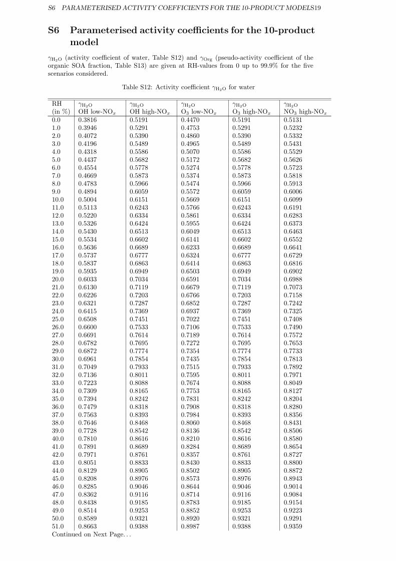
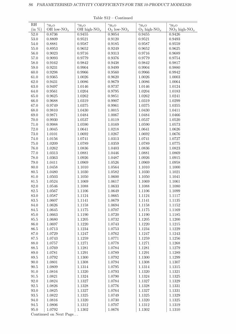
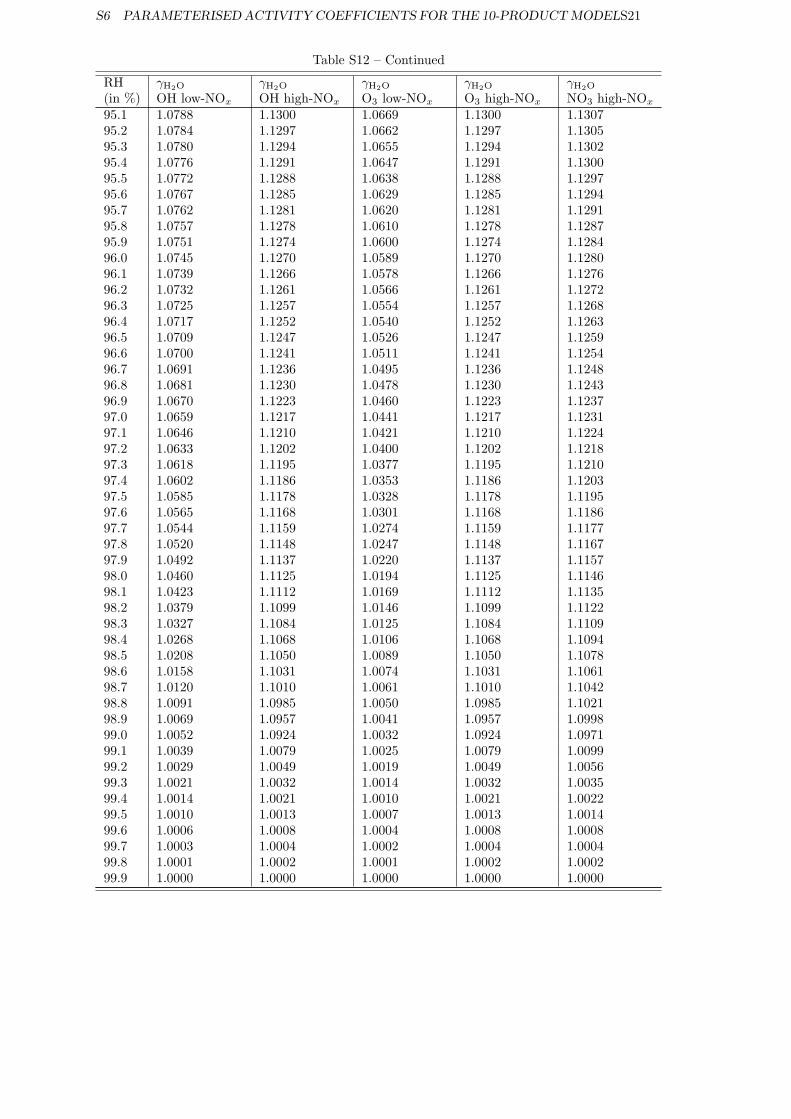
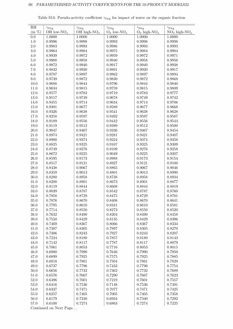
S6 Parameterised activity coefficients for the 10-productmodel
γH2O (activity coefficient of water, Table S12) and γOrg (pseudo-activity coefficient of theorganic SOA fraction, Table S13) are given at RH-values from 0 up to 99.9% for the fivescenarios considered.
Table S12: Activity coefficient γH2O for water
RH γH2O γH2O γH2O γH2O γH2O
(in %) OH low-NOx OH high-NOx O3 low-NOx O3 high-NOx NO3 high-NOx
0.0 0.3816 0.5191 0.4470 0.5191 0.51311.0 0.3946 0.5291 0.4753 0.5291 0.52322.0 0.4072 0.5390 0.4860 0.5390 0.53323.0 0.4196 0.5489 0.4965 0.5489 0.54314.0 0.4318 0.5586 0.5070 0.5586 0.55295.0 0.4437 0.5682 0.5172 0.5682 0.56266.0 0.4554 0.5778 0.5274 0.5778 0.57237.0 0.4669 0.5873 0.5374 0.5873 0.58188.0 0.4783 0.5966 0.5474 0.5966 0.59139.0 0.4894 0.6059 0.5572 0.6059 0.600610.0 0.5004 0.6151 0.5669 0.6151 0.609911.0 0.5113 0.6243 0.5766 0.6243 0.619112.0 0.5220 0.6334 0.5861 0.6334 0.628313.0 0.5326 0.6424 0.5955 0.6424 0.637314.0 0.5430 0.6513 0.6049 0.6513 0.646315.0 0.5534 0.6602 0.6141 0.6602 0.655216.0 0.5636 0.6689 0.6233 0.6689 0.664117.0 0.5737 0.6777 0.6324 0.6777 0.672918.0 0.5837 0.6863 0.6414 0.6863 0.681619.0 0.5935 0.6949 0.6503 0.6949 0.690220.0 0.6033 0.7034 0.6591 0.7034 0.698821.0 0.6130 0.7119 0.6679 0.7119 0.707322.0 0.6226 0.7203 0.6766 0.7203 0.715823.0 0.6321 0.7287 0.6852 0.7287 0.724224.0 0.6415 0.7369 0.6937 0.7369 0.732525.0 0.6508 0.7451 0.7022 0.7451 0.740826.0 0.6600 0.7533 0.7106 0.7533 0.749027.0 0.6691 0.7614 0.7189 0.7614 0.757228.0 0.6782 0.7695 0.7272 0.7695 0.765329.0 0.6872 0.7774 0.7354 0.7774 0.773330.0 0.6961 0.7854 0.7435 0.7854 0.781331.0 0.7049 0.7933 0.7515 0.7933 0.789232.0 0.7136 0.8011 0.7595 0.8011 0.797133.0 0.7223 0.8088 0.7674 0.8088 0.804934.0 0.7309 0.8165 0.7753 0.8165 0.812735.0 0.7394 0.8242 0.7831 0.8242 0.820436.0 0.7479 0.8318 0.7908 0.8318 0.828037.0 0.7563 0.8393 0.7984 0.8393 0.835638.0 0.7646 0.8468 0.8060 0.8468 0.843139.0 0.7728 0.8542 0.8136 0.8542 0.850640.0 0.7810 0.8616 0.8210 0.8616 0.858041.0 0.7891 0.8689 0.8284 0.8689 0.865442.0 0.7971 0.8761 0.8357 0.8761 0.872743.0 0.8051 0.8833 0.8430 0.8833 0.880044.0 0.8129 0.8905 0.8502 0.8905 0.887245.0 0.8208 0.8976 0.8573 0.8976 0.894346.0 0.8285 0.9046 0.8644 0.9046 0.901447.0 0.8362 0.9116 0.8714 0.9116 0.908448.0 0.8438 0.9185 0.8783 0.9185 0.915449.0 0.8514 0.9253 0.8852 0.9253 0.922350.0 0.8589 0.9321 0.8920 0.9321 0.929151.0 0.8663 0.9388 0.8987 0.9388 0.9359Continued on Next Page. . .
S6 PARAMETERISED ACTIVITY COEFFICIENTS FOR THE 10-PRODUCTMODELS20
Table S12 – Continued
RH γH2O γH2O γH2O γH2O γH2O
(in %) OH low-NOx OH high-NOx O3 low-NOx O3 high-NOx NO3 high-NOx
52.0 0.8736 0.9455 0.9054 0.9455 0.942653.0 0.8809 0.9521 0.9120 0.9521 0.949354.0 0.8881 0.9587 0.9185 0.9587 0.955955.0 0.8953 0.9652 0.9249 0.9652 0.962556.0 0.9023 0.9716 0.9313 0.9716 0.968957.0 0.9093 0.9779 0.9376 0.9779 0.975458.0 0.9162 0.9842 0.9438 0.9842 0.981759.0 0.9231 0.9904 0.9499 0.9904 0.988060.0 0.9298 0.9966 0.9560 0.9966 0.994261.0 0.9365 1.0026 0.9620 1.0026 1.000362.0 0.9431 1.0086 0.9679 1.0086 1.006463.0 0.9497 1.0146 0.9737 1.0146 1.012464.0 0.9561 1.0204 0.9795 1.0204 1.018365.0 0.9625 1.0262 0.9851 1.0262 1.024166.0 0.9688 1.0319 0.9907 1.0319 1.029967.0 0.9749 1.0375 0.9961 1.0375 1.035568.0 0.9810 1.0430 1.0015 1.0430 1.041169.0 0.9871 1.0484 1.0067 1.0484 1.046670.0 0.9930 1.0537 1.0119 1.0537 1.052071.0 0.9988 1.0590 1.0169 1.0590 1.057372.0 1.0045 1.0641 1.0218 1.0641 1.062673.0 1.0101 1.0692 1.0267 1.0692 1.067674.0 1.0156 1.0741 1.0313 1.0741 1.072775.0 1.0209 1.0789 1.0359 1.0789 1.077576.0 1.0262 1.0836 1.0403 1.0836 1.082377.0 1.0313 1.0881 1.0446 1.0881 1.086978.0 1.0363 1.0926 1.0487 1.0926 1.091579.0 1.0411 1.0969 1.0526 1.0969 1.095880.0 1.0458 1.1010 1.0564 1.1010 1.100080.5 1.0480 1.1030 1.0582 1.1030 1.102181.0 1.0503 1.1050 1.0600 1.1050 1.104181.5 1.0524 1.1069 1.0617 1.1069 1.106182.0 1.0546 1.1088 1.0633 1.1088 1.108082.5 1.0567 1.1106 1.0649 1.1106 1.109983.0 1.0587 1.1124 1.0665 1.1124 1.111783.5 1.0607 1.1141 1.0679 1.1141 1.113584.0 1.0626 1.1158 1.0694 1.1158 1.115284.5 1.0645 1.1175 1.0707 1.1175 1.116985.0 1.0663 1.1190 1.0720 1.1190 1.118585.5 1.0680 1.1205 1.0732 1.1205 1.120086.0 1.0697 1.1220 1.0743 1.1220 1.121586.5 1.0713 1.1234 1.0753 1.1234 1.122987.0 1.0729 1.1247 1.0762 1.1247 1.124387.5 1.0743 1.1259 1.0771 1.1259 1.125688.0 1.0757 1.1271 1.0778 1.1271 1.126888.5 1.0769 1.1281 1.0784 1.1281 1.127989.0 1.0781 1.1291 1.0789 1.1291 1.128989.5 1.0792 1.1300 1.0792 1.1300 1.129990.0 1.0801 1.1308 1.0794 1.1308 1.130790.5 1.0809 1.1314 1.0795 1.1314 1.131591.0 1.0816 1.1320 1.0793 1.1320 1.132191.5 1.0821 1.1324 1.0790 1.1324 1.132592.0 1.0824 1.1327 1.0784 1.1327 1.132992.5 1.0826 1.1328 1.0776 1.1328 1.133193.0 1.0825 1.1327 1.0764 1.1327 1.133193.5 1.0822 1.1325 1.0749 1.1325 1.132994.0 1.0816 1.1320 1.0730 1.1320 1.132594.5 1.0806 1.1312 1.0707 1.1312 1.131995.0 1.0792 1.1302 1.0676 1.1302 1.1310Continued on Next Page. . .
S6 PARAMETERISED ACTIVITY COEFFICIENTS FOR THE 10-PRODUCTMODELS21
Table S12 – Continued
RH γH2O γH2O γH2O γH2O γH2O
(in %) OH low-NOx OH high-NOx O3 low-NOx O3 high-NOx NO3 high-NOx
95.1 1.0788 1.1300 1.0669 1.1300 1.130795.2 1.0784 1.1297 1.0662 1.1297 1.130595.3 1.0780 1.1294 1.0655 1.1294 1.130295.4 1.0776 1.1291 1.0647 1.1291 1.130095.5 1.0772 1.1288 1.0638 1.1288 1.129795.6 1.0767 1.1285 1.0629 1.1285 1.129495.7 1.0762 1.1281 1.0620 1.1281 1.129195.8 1.0757 1.1278 1.0610 1.1278 1.128795.9 1.0751 1.1274 1.0600 1.1274 1.128496.0 1.0745 1.1270 1.0589 1.1270 1.128096.1 1.0739 1.1266 1.0578 1.1266 1.127696.2 1.0732 1.1261 1.0566 1.1261 1.127296.3 1.0725 1.1257 1.0554 1.1257 1.126896.4 1.0717 1.1252 1.0540 1.1252 1.126396.5 1.0709 1.1247 1.0526 1.1247 1.125996.6 1.0700 1.1241 1.0511 1.1241 1.125496.7 1.0691 1.1236 1.0495 1.1236 1.124896.8 1.0681 1.1230 1.0478 1.1230 1.124396.9 1.0670 1.1223 1.0460 1.1223 1.123797.0 1.0659 1.1217 1.0441 1.1217 1.123197.1 1.0646 1.1210 1.0421 1.1210 1.122497.2 1.0633 1.1202 1.0400 1.1202 1.121897.3 1.0618 1.1195 1.0377 1.1195 1.121097.4 1.0602 1.1186 1.0353 1.1186 1.120397.5 1.0585 1.1178 1.0328 1.1178 1.119597.6 1.0565 1.1168 1.0301 1.1168 1.118697.7 1.0544 1.1159 1.0274 1.1159 1.117797.8 1.0520 1.1148 1.0247 1.1148 1.116797.9 1.0492 1.1137 1.0220 1.1137 1.115798.0 1.0460 1.1125 1.0194 1.1125 1.114698.1 1.0423 1.1112 1.0169 1.1112 1.113598.2 1.0379 1.1099 1.0146 1.1099 1.112298.3 1.0327 1.1084 1.0125 1.1084 1.110998.4 1.0268 1.1068 1.0106 1.1068 1.109498.5 1.0208 1.1050 1.0089 1.1050 1.107898.6 1.0158 1.1031 1.0074 1.1031 1.106198.7 1.0120 1.1010 1.0061 1.1010 1.104298.8 1.0091 1.0985 1.0050 1.0985 1.102198.9 1.0069 1.0957 1.0041 1.0957 1.099899.0 1.0052 1.0924 1.0032 1.0924 1.097199.1 1.0039 1.0079 1.0025 1.0079 1.009999.2 1.0029 1.0049 1.0019 1.0049 1.005699.3 1.0021 1.0032 1.0014 1.0032 1.003599.4 1.0014 1.0021 1.0010 1.0021 1.002299.5 1.0010 1.0013 1.0007 1.0013 1.001499.6 1.0006 1.0008 1.0004 1.0008 1.000899.7 1.0003 1.0004 1.0002 1.0004 1.000499.8 1.0001 1.0002 1.0001 1.0002 1.000299.9 1.0000 1.0000 1.0000 1.0000 1.0000
S6 PARAMETERISED ACTIVITY COEFFICIENTS FOR THE 10-PRODUCTMODELS22
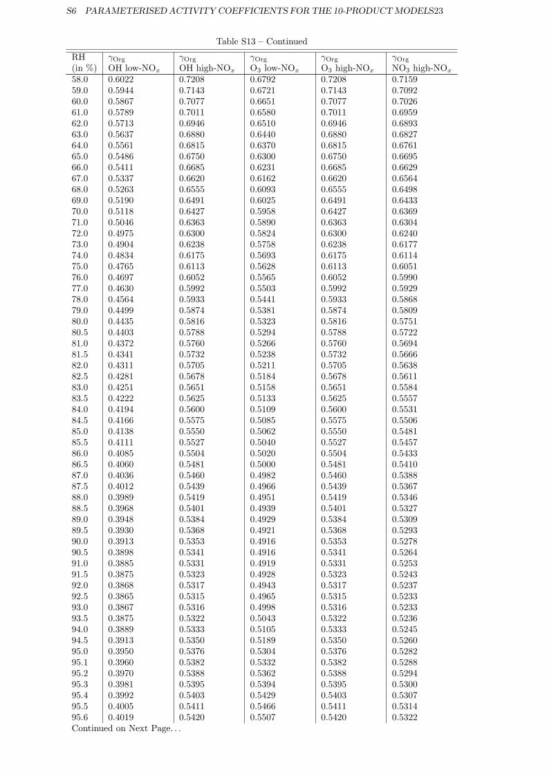
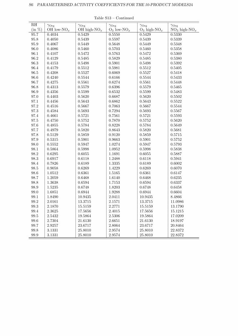
Table S13: Pseudo-activity coefficient γOrg for impact of water on the organic fraction
RH γOrg γOrg γOrg γOrg γOrg
(in %) OH low-NOx OH high-NOx O3 low-NOx O3 high-NOx NO3 high-NOx
0.0 1.0000 1.0000 1.0000 1.0000 1.00001.0 0.9996 0.9998 0.9993 0.9998 0.99982.0 0.9983 0.9993 0.9986 0.9993 0.99933.0 0.9964 0.9984 0.9975 0.9984 0.99844.0 0.9939 0.9972 0.9959 0.9972 0.99715.0 0.9908 0.9958 0.9940 0.9958 0.99566.0 0.9872 0.9940 0.9917 0.9940 0.99387.0 0.9832 0.9920 0.9891 0.9920 0.99178.0 0.9787 0.9897 0.9862 0.9897 0.98949.0 0.9739 0.9872 0.9830 0.9872 0.986810.0 0.9688 0.9844 0.9796 0.9844 0.984011.0 0.9634 0.9815 0.9759 0.9815 0.980912.0 0.9577 0.9783 0.9719 0.9783 0.977713.0 0.9517 0.9749 0.9678 0.9749 0.974214.0 0.9455 0.9714 0.9634 0.9714 0.970615.0 0.9391 0.9677 0.9589 0.9677 0.966816.0 0.9326 0.9638 0.9541 0.9638 0.962817.0 0.9258 0.9597 0.9492 0.9597 0.958718.0 0.9189 0.9556 0.9442 0.9556 0.954419.0 0.9119 0.9512 0.9389 0.9512 0.950020.0 0.9047 0.9467 0.9336 0.9467 0.945421.0 0.8974 0.9421 0.9281 0.9421 0.940722.0 0.8900 0.9374 0.9224 0.9374 0.935823.0 0.8825 0.9325 0.9167 0.9325 0.930924.0 0.8749 0.9276 0.9109 0.9276 0.925825.0 0.8672 0.9225 0.9049 0.9225 0.920726.0 0.8595 0.9173 0.8988 0.9173 0.915427.0 0.8517 0.9121 0.8927 0.9121 0.910028.0 0.8438 0.9067 0.8865 0.9067 0.904629.0 0.8359 0.9013 0.8801 0.9013 0.899030.0 0.8280 0.8958 0.8738 0.8958 0.893431.0 0.8200 0.8901 0.8673 0.8901 0.887732.0 0.8119 0.8844 0.8608 0.8844 0.881933.0 0.8039 0.8787 0.8542 0.8787 0.876034.0 0.7958 0.8729 0.8475 0.8729 0.870135.0 0.7876 0.8670 0.8408 0.8670 0.864136.0 0.7795 0.8610 0.8341 0.8610 0.858137.0 0.7714 0.8550 0.8273 0.8550 0.852038.0 0.7632 0.8490 0.8204 0.8490 0.845839.0 0.7550 0.8429 0.8135 0.8429 0.839640.0 0.7469 0.8367 0.8066 0.8367 0.833441.0 0.7387 0.8305 0.7997 0.8305 0.827042.0 0.7306 0.8243 0.7927 0.8243 0.820743.0 0.7224 0.8180 0.7857 0.8180 0.814344.0 0.7142 0.8117 0.7787 0.8117 0.807945.0 0.7061 0.8053 0.7716 0.8053 0.801546.0 0.6980 0.7990 0.7646 0.7990 0.795047.0 0.6899 0.7925 0.7575 0.7925 0.788548.0 0.6818 0.7861 0.7504 0.7861 0.782049.0 0.6737 0.7796 0.7433 0.7796 0.775450.0 0.6656 0.7732 0.7362 0.7732 0.768951.0 0.6576 0.7667 0.7290 0.7667 0.762352.0 0.6496 0.7601 0.7219 0.7601 0.755753.0 0.6416 0.7536 0.7148 0.7536 0.749154.0 0.6337 0.7471 0.7077 0.7471 0.742555.0 0.6257 0.7405 0.7005 0.7405 0.735856.0 0.6179 0.7340 0.6934 0.7340 0.729257.0 0.6100 0.7274 0.6863 0.7274 0.7225Continued on Next Page. . .
S6 PARAMETERISED ACTIVITY COEFFICIENTS FOR THE 10-PRODUCTMODELS23
Table S13 – Continued
RH γOrg γOrg γOrg γOrg γOrg
(in %) OH low-NOx OH high-NOx O3 low-NOx O3 high-NOx NO3 high-NOx
58.0 0.6022 0.7208 0.6792 0.7208 0.715959.0 0.5944 0.7143 0.6721 0.7143 0.709260.0 0.5867 0.7077 0.6651 0.7077 0.702661.0 0.5789 0.7011 0.6580 0.7011 0.695962.0 0.5713 0.6946 0.6510 0.6946 0.689363.0 0.5637 0.6880 0.6440 0.6880 0.682764.0 0.5561 0.6815 0.6370 0.6815 0.676165.0 0.5486 0.6750 0.6300 0.6750 0.669566.0 0.5411 0.6685 0.6231 0.6685 0.662967.0 0.5337 0.6620 0.6162 0.6620 0.656468.0 0.5263 0.6555 0.6093 0.6555 0.649869.0 0.5190 0.6491 0.6025 0.6491 0.643370.0 0.5118 0.6427 0.5958 0.6427 0.636971.0 0.5046 0.6363 0.5890 0.6363 0.630472.0 0.4975 0.6300 0.5824 0.6300 0.624073.0 0.4904 0.6238 0.5758 0.6238 0.617774.0 0.4834 0.6175 0.5693 0.6175 0.611475.0 0.4765 0.6113 0.5628 0.6113 0.605176.0 0.4697 0.6052 0.5565 0.6052 0.599077.0 0.4630 0.5992 0.5503 0.5992 0.592978.0 0.4564 0.5933 0.5441 0.5933 0.586879.0 0.4499 0.5874 0.5381 0.5874 0.580980.0 0.4435 0.5816 0.5323 0.5816 0.575180.5 0.4403 0.5788 0.5294 0.5788 0.572281.0 0.4372 0.5760 0.5266 0.5760 0.569481.5 0.4341 0.5732 0.5238 0.5732 0.566682.0 0.4311 0.5705 0.5211 0.5705 0.563882.5 0.4281 0.5678 0.5184 0.5678 0.561183.0 0.4251 0.5651 0.5158 0.5651 0.558483.5 0.4222 0.5625 0.5133 0.5625 0.555784.0 0.4194 0.5600 0.5109 0.5600 0.553184.5 0.4166 0.5575 0.5085 0.5575 0.550685.0 0.4138 0.5550 0.5062 0.5550 0.548185.5 0.4111 0.5527 0.5040 0.5527 0.545786.0 0.4085 0.5504 0.5020 0.5504 0.543386.5 0.4060 0.5481 0.5000 0.5481 0.541087.0 0.4036 0.5460 0.4982 0.5460 0.538887.5 0.4012 0.5439 0.4966 0.5439 0.536788.0 0.3989 0.5419 0.4951 0.5419 0.534688.5 0.3968 0.5401 0.4939 0.5401 0.532789.0 0.3948 0.5384 0.4929 0.5384 0.530989.5 0.3930 0.5368 0.4921 0.5368 0.529390.0 0.3913 0.5353 0.4916 0.5353 0.527890.5 0.3898 0.5341 0.4916 0.5341 0.526491.0 0.3885 0.5331 0.4919 0.5331 0.525391.5 0.3875 0.5323 0.4928 0.5323 0.524392.0 0.3868 0.5317 0.4943 0.5317 0.523792.5 0.3865 0.5315 0.4965 0.5315 0.523393.0 0.3867 0.5316 0.4998 0.5316 0.523393.5 0.3875 0.5322 0.5043 0.5322 0.523694.0 0.3889 0.5333 0.5105 0.5333 0.524594.5 0.3913 0.5350 0.5189 0.5350 0.526095.0 0.3950 0.5376 0.5304 0.5376 0.528295.1 0.3960 0.5382 0.5332 0.5382 0.528895.2 0.3970 0.5388 0.5362 0.5388 0.529495.3 0.3981 0.5395 0.5394 0.5395 0.530095.4 0.3992 0.5403 0.5429 0.5403 0.530795.5 0.4005 0.5411 0.5466 0.5411 0.531495.6 0.4019 0.5420 0.5507 0.5420 0.5322Continued on Next Page. . .
S6 PARAMETERISED ACTIVITY COEFFICIENTS FOR THE 10-PRODUCTMODELS24
Table S13 – Continued
RH γOrg γOrg γOrg γOrg γOrg
(in %) OH low-NOx OH high-NOx O3 low-NOx O3 high-NOx NO3 high-NOx
95.7 0.4034 0.5429 0.5550 0.5429 0.533095.8 0.4050 0.5439 0.5597 0.5439 0.533995.9 0.4067 0.5449 0.5648 0.5449 0.534896.0 0.4086 0.5460 0.5703 0.5460 0.535896.1 0.4107 0.5472 0.5763 0.5472 0.536996.2 0.4129 0.5485 0.5829 0.5485 0.538096.3 0.4153 0.5498 0.5901 0.5498 0.539296.4 0.4179 0.5512 0.5981 0.5512 0.540596.5 0.4208 0.5527 0.6069 0.5527 0.541896.6 0.4240 0.5544 0.6166 0.5544 0.543396.7 0.4275 0.5561 0.6274 0.5561 0.544896.8 0.4313 0.5579 0.6396 0.5579 0.546596.9 0.4356 0.5599 0.6532 0.5599 0.548397.0 0.4403 0.5620 0.6687 0.5620 0.550297.1 0.4456 0.5643 0.6862 0.5643 0.552297.2 0.4516 0.5667 0.7063 0.5667 0.554497.3 0.4584 0.5693 0.7294 0.5693 0.556797.4 0.4661 0.5721 0.7561 0.5721 0.559397.5 0.4750 0.5752 0.7870 0.5752 0.562097.6 0.4855 0.5784 0.8228 0.5784 0.564997.7 0.4979 0.5820 0.8643 0.5820 0.568197.8 0.5129 0.5859 0.9120 0.5859 0.571597.9 0.5315 0.5901 0.9663 0.5901 0.575298.0 0.5552 0.5947 1.0274 0.5947 0.579398.1 0.5864 0.5998 1.0952 0.5998 0.583898.2 0.6295 0.6055 1.1691 0.6055 0.588798.3 0.6917 0.6118 1.2488 0.6118 0.594198.4 0.7826 0.6189 1.3335 0.6189 0.600298.5 0.9058 0.6269 1.4229 0.6269 0.607098.6 1.0512 0.6361 1.5165 0.6361 0.614798.7 1.2059 0.6468 1.6140 0.6468 0.623598.8 1.3638 0.6594 1.7153 0.6594 0.633798.9 1.5235 0.6748 1.8203 0.6748 0.645899.0 1.6851 0.6944 1.9288 0.6944 0.660499.1 1.8490 10.9435 2.0411 10.9435 8.486699.2 2.0161 13.3715 2.1571 13.3715 11.098699.3 2.1870 15.5159 2.2771 15.5159 13.179099.4 2.3625 17.5656 2.4015 17.5656 15.121599.5 2.5432 19.5864 2.5306 19.5864 17.020999.6 2.7304 21.6130 2.6651 21.6130 18.919799.7 2.9257 23.6717 2.8064 23.6717 20.846499.8 3.1331 25.8010 2.9574 25.8010 22.837299.9 3.1331 25.8010 2.9574 25.8010 22.8372
S7 COMPARISONOF THE PARAMETERISATION FOR RH-DEPENDENCE AT INTERMEDIATE NOXS25
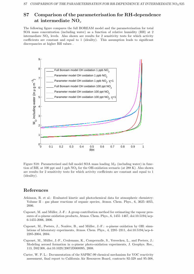
S7 Comparison of the parameterisation for RH-dependenceat intermediate NOx
The following figure compares the full BOREAM model and the parameterisation for totalSOA mass concentration (including water) as a function of relative humidity (RH) at 2intermediate NOx levels. Also shown are results for 2 sensitivity tests for which activitycoefficients are constant and equal to 1 (ideality). This assumption leads to significantdiscrepancies at higher RH values .
0 0.1 0.2 0.3 0.4 0.5 0.6 0.7 0.8 0.9 10
1
2
3
4
5
6
7
8
9
RH
MO
incl
udin
g w
ater
(in
µ g
m−
3 )
Full Boream model OH oxidation 1 ppb NO2
Parameter model OH oxidation 1 ppb NO2
Parameter model OH oxidation 1 ppb NO2, γ
i=1
Full Boream model OH oxidation 100 ppt NO2
Parameter model OH oxidation 100 ppt NO2
Parameter model OH oxidation 100 ppt NO2, γ
i=1
Figure S18: Parameterised and full model SOA mass loading MO (including water) in func-tion of RH, at 100 ppt and 1 ppb NO2 for the OH-oxidation scenario (at 288 K). Also shownare results for 2 sensitivity tests for which activity coefficients are constant and equal to 1(ideality).
References
Atkinson, R. et al.: Evaluated kinetic and photochemical data for atmospheric chemistry:Volume II - gas phase reactions of organic species, Atmos. Chem. Phys., 6, 3625–4055,2006.
Capouet, M. and Muller, J.-F.: A group contribution method for estimating the vapour pres-sures of α-pinene oxidation products, Atmos. Chem. Phys., 6, 1455–1467, doi:10.5194/acp-6-1455-2006, 2006.
Capouet, M., Peeters, J., Noziere, B., and Muller, J.-F.: α-pinene oxidation by OH: simu-lations of laboratory experiments, Atmos. Chem. Phys., 4, 2285–2311, doi:10.5194/acp-4-2285-2004, 2004.
Capouet, M., Muller, J.-F., Ceulemans, K., Compernolle, S., Vereecken, L., and Peeters, J.:Modeling aerosol formation in α-pinene photo-oxidation experiments, J. Geophys. Res.,113, D02 308, doi:10.1029/2007JD008995, 2008.
Carter, W. P. L.: Documentation of the SAPRC-99 chemical mechanism for VOC reactivityassessment, final report to California Air Resources Board, contracts 92-329 and 95-308,
REFERENCES S26
Tech. rep., Air Pollut. Res. Cent.for Environ. Res. and Technol., Univ. of California,Riverside, California, URL http://.www.cert.ucr.edu/ carter/reactdat.htm, 2000.
Ceulemans, K., Compernolle, S., Peeters, J., and Muller, J.-F.: Evaluation of a detailedmodel of secondary organic aerosol formation from α-pinene against dark ozonolysis ex-periments, Atmos. Environ., 44, 5434–5442, doi:10.5194/acp-9-1325-2009, 2010.
Jenkin, M. E., Hurley, M. D., and Wallington, T. J.: Investigation of the radical productchannel of the CH3C(O)O2 + HO2 reaction in the gas phase, Phys. Chem. Chem. Phys.,9, 3149–3162, 2007.
Makar, P. A.: The estimation of organic gas vapour pressure, Atmos. Environ., 35, 961–974,2001.
Neeb, P.: Structure-reactivity based estimation of the rate constants for hydroxyl radicalreactions with hydrocarbons, J. Atmos. Chem., 35, 295–315, 2000.
Ng, N. L., Chhabra, P. S., Chan, A. W. H., Surratt, J. D., Kroll, J. H., Kwan, A. J., McCabe,D. C., Wennberg, P. O., Sorooshian, A., Murphy, S. M., Dalleska, N. F., Flagan, R. C.,and Seinfeld, J. H.: Effect of NOx level on secondary organic aerosol (SOA) formationfrom the photooxidation of terpenes, Atmos. Chem. Phys., 7, 5159–5174, doi:10.5194/acp-7-5159-2007, 2007.
Paulson, S. E., Liu, D.-L., and Orzechowska, G. E.: Photolysis of heptanal, J. Org. Chem.,71, 6403–6408, 2006.
Saunders, S. M., Jenkin, M. E., Derwent, R. G., and Pilling, M. J.: Protocol for the devel-opment of the Master Chemical Mechanism, MCM v3 (Part A): tropospheric degradationof non-aromatic volatile organic compounds, Atmos. Chem. Phys., 3, 161–180, 2003.
Schurath, U. and Naumann, K.-H.: Chemical Mechanism Develoment (CMD), EUROTRAC-2 subproject, final report, Tech. rep., Int. Sci. Secr.t, GSF-Natl. Res. Cent. for Environ.and Health, Munich, Germany, 2003.
Valorso, R., Aumont, B., Camredon, M., Raventos-Duran, T., Mouchel-Vallon, C., Ng, N. L.,Seinfeld, J. H., Lee-Taylor, J., and Madronich, S.: Explicit modelling of SOA formationfrom α-pinene photooxidation: sensitivity to vapour pressure estimation, Atmos. Chem.Phys., 11, 68956910, doi:10.5194/acp-11-6895-2011, 2011.
Vereecken, L. and Peeters, J.: Decomposition of substituted alkoxy radicals - part 1: ageneralized structure-activity relationship for reaction barrier heights, Phys. Chem. Chem.Phys., 11, 9062–9074, 2009.