Statistical Physics M. Flohr & G. Palacios 07.12.2005 1

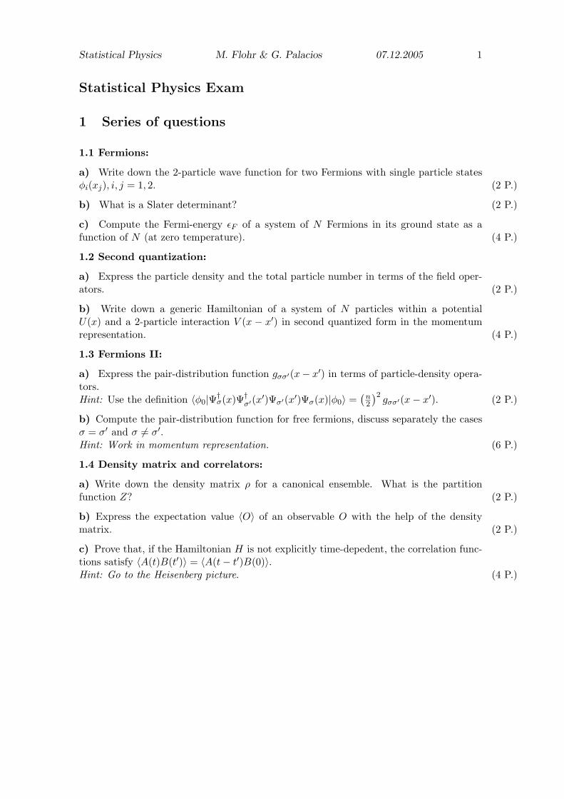
Statistical Physics Exam

1 Series of questions

1.1 Fermions:

a) Write down the 2-particle wave function for two Fermions with single particle statesφi(xj), i, j = 1, 2. (2 P.)

b) What is a Slater determinant? (2 P.)

c) Compute the Fermi-energy εF of a system of N Fermions in its ground state as afunction of N (at zero temperature). (4 P.)

1.2 Second quantization:

a) Express the particle density and the total particle number in terms of the field oper-ators. (2 P.)

b) Write down a generic Hamiltonian of a system of N particles within a potentialU(x) and a 2-particle interaction V (x − x′) in second quantized form in the momentumrepresentation. (4 P.)

1.3 Fermions II:

a) Express the pair-distribution function gσσ′(x− x′) in terms of particle-density opera-tors.Hint: Use the definition 〈φ0|Ψ†

σ(x)Ψ†σ′(x′)Ψσ′(x′)Ψσ(x)|φ0〉 =

(n2

)2gσσ′(x− x′). (2 P.)

b) Compute the pair-distribution function for free fermions, discuss separately the casesσ = σ′ and σ 6= σ′.Hint: Work in momentum representation. (6 P.)

1.4 Density matrix and correlators:

a) Write down the density matrix ρ for a canonical ensemble. What is the partitionfunction Z? (2 P.)

b) Express the expectation value 〈O〉 of an observable O with the help of the densitymatrix. (2 P.)

c) Prove that, if the Hamiltonian H is not explicitly time-depedent, the correlation func-tions satisfy 〈A(t)B(t′)〉 = 〈A(t− t′)B(0)〉.Hint: Go to the Heisenberg picture. (4 P.)

Statistical Physics M. Flohr & G. Palacios 07.12.2005 2

2 Exercices

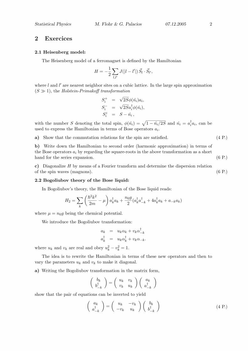
2.1 Heisenberg model:

The Heisenberg model of a ferromagnet is defined by the Hamiltonian

H = −12

∑l,l′

J(|l − l′|) ~Sl · ~Sl′ ,

where l and l′ are nearest neighbor sites on a cubic lattice. In the large spin approximation(S � 1), the Holstein-Primakoff transformation

S+i =

√2Sφ(n̂i)ai,

S−i =

√2Sa†iφ(n̂i),

Szi = S − n̂i ,

with the number S denoting the total spin, φ(n̂i) =√

1− n̂i/2S and n̂i = a†iai, can beused to express the Hamiltonian in terms of Bose operators ai.

a) Show that the commutation relations for the spin are satisfied. (4 P.)

b) Write down the Hamiltonian to second order (harmonic approximation) in terms ofthe Bose operators ai by regarding the square-roots in the above transformation as a shorthand for the series expansion. (6 P.)

c) Diagonalize H by means of a Fourier transform and determine the dispersion relationof the spin waves (magnons). (6 P.)

2.2 Bogoliubov theory of the Bose liquid:

In Bogoliubov’s theory, the Hamiltonian of the Bose liquid reads:

H2 =∑

k

(~2k2

2m− µ

)a†kak +

n0g

2(a†ka

†−k + 4a†kak + a−kak)

where µ = n0g being the chemical potential.

We introduce the Bogoliubov transformation:

ak = ukαk + vkα†−k

a†k = ukα†k + vkα−k.

where uk and vk are real and obey u2k − v2

k = 1.

The idea is to rewrite the Hamiltonian in terms of these new operators and then tovary the parameters uk and vk to make it diagonal.

a) Writing the Bogoliubov transformation in the matrix form,(bk

b†−k

)=

(uk vk

vk uk

) (ak

a†−k

)show that the pair of equations can be inverted to yield(

ak

a†−k

)=

(uk −vk

−vk uk

) (bk

b†−k

)(4 P.)

Statistical Physics M. Flohr & G. Palacios 07.12.2005 3

b) Rewrite the Hamiltonian H2 in the matrix form

H2 =∑

k

(a†k a−k

) (εk + n0g n0g/2n0g/2 0

) (ak

a†−k

)where εk = ~2k2/2m. (4 P.)

c) Use the inverse of the Bogoliubov transformation to express H2 in terms of the b′soperators, namely you should find:

H2 =∑

k

(b†k b−k

) (M11 M12

M21 M22

) (bk

b†−k

)where the coefficients Mij have to be computed explicitly. (8 P.)

d) Show that the condition for the transformed matrix to be diagonal is that

2ukvk

u2k + v2

k

=n0g

εk + n0g

must be satisfied. (4 P.)

e) Show that the trace of the M matrix is

E = (εk + n0g)(u2k + v2

k)− 2n0gukvk .

Using the representation uk = cosh(θ) and vk = sinh(θ), show from d) that

tanh(2θ) =n0g

εk + n0g

and hence prove thatE =

√εk(εk + 2n0g) ,

consistent with the Bogoliubov quasiparticle dispersion given in the lecture. (4 P.)

Total: (70 P.)