Statistical Physics

Gavin CheungF

May 11, 2012

Contents

1 Thermodynamics 4

1.1 Clausius-Clapeyron Equation Derivation . . . . . . . . . . . . . . . . . . . 4

2 Framework for Statistical Physics 5

2.1 Γ-Space . . . . . . . . . . . . . . . . . . . . . . . . . . . . . . . . . . . . . 5

2.2 µ-space . . . . . . . . . . . . . . . . . . . . . . . . . . . . . . . . . . . . . . 6

2.3 Microstates and Macrostates . . . . . . . . . . . . . . . . . . . . . . . . . . 6

2.4 Ergodic Hypothesis . . . . . . . . . . . . . . . . . . . . . . . . . . . . . . . 6

2.5 Distribution Function . . . . . . . . . . . . . . . . . . . . . . . . . . . . . . 6

3 Ensembles 8

3.1 Entropy . . . . . . . . . . . . . . . . . . . . . . . . . . . . . . . . . . . . . 8

3.2 Statistical Ensembles . . . . . . . . . . . . . . . . . . . . . . . . . . . . . . 8

3.3 Microcanonical Ensemble . . . . . . . . . . . . . . . . . . . . . . . . . . . . 9

4 Canonical Ensemble 12

4.1 Connection with Thermodynamics . . . . . . . . . . . . . . . . . . . . . . . 13

4.2 β = 1kT

. . . . . . . . . . . . . . . . . . . . . . . . . . . . . . . . . . . . . . 14

4.3 The Ideal Gas . . . . . . . . . . . . . . . . . . . . . . . . . . . . . . . . . . 14

4.4 Equipartition of Energy . . . . . . . . . . . . . . . . . . . . . . . . . . . . 15

5 Grand Canonical Ensemble 16

1

5.1 Thermodynamics . . . . . . . . . . . . . . . . . . . . . . . . . . . . . . . . 17

5.2 Grand Canonical Potential . . . . . . . . . . . . . . . . . . . . . . . . . . . 18

5.3 The Ideal Gas . . . . . . . . . . . . . . . . . . . . . . . . . . . . . . . . . . 18

6 An Interacting Gas 20

6.1 Computing the Partition Function . . . . . . . . . . . . . . . . . . . . . . . 21

6.2 Cluster Expansion . . . . . . . . . . . . . . . . . . . . . . . . . . . . . . . 22

7 Magnetism 23

8 Quantum Statistical Mechanics 25

8.1 Time Evolution of the Density Operator . . . . . . . . . . . . . . . . . . . 26

8.2 Partition Functions . . . . . . . . . . . . . . . . . . . . . . . . . . . . . . . 28

9 Identical Particles 30

9.1 Bose-Einstein Distribution . . . . . . . . . . . . . . . . . . . . . . . . . . . 31

9.2 Fermi-Dirac Distribution . . . . . . . . . . . . . . . . . . . . . . . . . . . . 31

9.3 Expected Occupation Numbers . . . . . . . . . . . . . . . . . . . . . . . . 32

10 Ideal Quantum Gas 33

10.1 Density of States . . . . . . . . . . . . . . . . . . . . . . . . . . . . . . . . 33

11 Fermi Gas 35

11.1 Fermi Gas at Zero Temperature . . . . . . . . . . . . . . . . . . . . . . . . 37

11.2 Fermi Gas near Zero Temperature . . . . . . . . . . . . . . . . . . . . . . . 38

11.3 Entropy . . . . . . . . . . . . . . . . . . . . . . . . . . . . . . . . . . . . . 39

11.4 Heat Capacity . . . . . . . . . . . . . . . . . . . . . . . . . . . . . . . . . . 40

12 Bose Gas 41

12.1 Bose Einstein Condensation . . . . . . . . . . . . . . . . . . . . . . . . . . 42

2

12.2 Equation of State for T < Tc . . . . . . . . . . . . . . . . . . . . . . . . . . 43

12.3 Equation of State for T > Tc . . . . . . . . . . . . . . . . . . . . . . . . . . 44

12.4 Heat Capacity . . . . . . . . . . . . . . . . . . . . . . . . . . . . . . . . . . 44

13 Heat Capacity of a Solid 47

13.1 Classical Heat Capacity of a Solid . . . . . . . . . . . . . . . . . . . . . . . 47

13.2 Einstein Model . . . . . . . . . . . . . . . . . . . . . . . . . . . . . . . . . 48

14 Blackbody Radiation 50

14.1 Relativistic Bose Gas . . . . . . . . . . . . . . . . . . . . . . . . . . . . . . 50

14.2 Photon Gas . . . . . . . . . . . . . . . . . . . . . . . . . . . . . . . . . . . 51

15 Magnetic Systems 53

15.1 Magnetic Susceptibility . . . . . . . . . . . . . . . . . . . . . . . . . . . . . 53

15.2 An Example of Paramagnetism . . . . . . . . . . . . . . . . . . . . . . . . 53

15.3 Paramagnetism and Diamagnetism . . . . . . . . . . . . . . . . . . . . . . 55

15.4 Electron Moving in a Magnetic Field with no Spin . . . . . . . . . . . . . . 55

15.5 Landau Diamagnetism . . . . . . . . . . . . . . . . . . . . . . . . . . . . . 56

15.6 De Haas-Van Alphen Effect . . . . . . . . . . . . . . . . . . . . . . . . . . 58

16 Ferromagnetism 60

16.1 Non-Interacting Case . . . . . . . . . . . . . . . . . . . . . . . . . . . . . . 61

16.2 Mean Field Approximation . . . . . . . . . . . . . . . . . . . . . . . . . . . 62

3

Chapter 1

Thermodynamics

1.1 Clausius-Clapeyron Equation Derivation

Consider 2 phases A and B that can coexist on some line. At this point, the Gibbs energyof the 2 phases are equal or,

dGA = dGB

Recalling that dG = −SdT + V dP + µdN ,

−SAdT + VAdP + µAdN = −SBdT + VBdP + µBdN

We have dN = 0 due to particle number conservation.

⇒ ∆SdT = ∆V dP

dP

dT=

∆s

∆v

where we have multiplied by MM

to get the specific values. Since latent heat is defined byl = TC∆s,

dP

dT=

l

TC∆v

This gives the slope of the line that separates the phases on a PT diagram. One immediateconsequence is that for a first order phase transition, the volume must change.

4

Chapter 2

Framework for Statistical Physics

The way we formulate statistical physics will be established in this section. The ideaof a state of a system will be established followed by a development of the distributionfunction.

2.1 Γ-Space

How do we classify the state of a system of N particles? In classical mechanics, a stateof a particle is specified by momentum and position; p, r. The vectors belong in a6-dimensional space called the phase space. For N particles, the phase space is 6N -dimensional. Denote (p1,p2, . . . ,pN , r1, . . . , rN) = (p, r). The Hamiltonian is,

H(p, r) =N∑i=1

p2i

2m+

1

2

∑i 6=j

V (ri − rj)

The half in front of the potential is to prevent double counting. Hamilton’s equations ofmotion govern how the particles move.

Definition: The 6N -dimensional space spanned by (p, r) is called the Γ-space. Apoint, (p, r), in this space is called a representative point.

As time evolves, a point traces out a trajectory in Γ-space. If the Hamiltonian has noexplicit dependence on time, then energy is conserved. The points, (p, r), are constrainedto a hypersurface H(p, r) = E in Γ-space.

5

2.2 µ-space

Another way to consider the motion of particles is to consider a 6-dimensional phasespace called the µ-space. Each particle is described by a point, (p1, p2, p3, x, y, z). For Nparticles, there are N points. These points evolve in time and can collide with each other.

To summarise, in Γ-space, N particles are described by a single point in 6N -dimensionalspace. In µ-space, N particles are described by N points in 6-dimensional space.

2.3 Microstates and Macrostates

A microstate is a state that specifies all the parameters of the system. In a system ofN particles, we know the position and momentum of each particle. The state can bedescribed by one of the spaces mentioned above.

A macrostate is a state that describes the system as whole. For example, a systemwith a fixed pressure, volume and temperature is a particular macrostate. There are manydifferent possible microstates that can give rise to a particular macrostate.

2.4 Ergodic Hypothesis

The ergodic hypothesis assumes,

“Given a sufficiently long time, the representative point of an isolated systemwill come arbitrarily close to any given point on the energy surface.”

Essentially, what we need from this is that all microstates that correspond to a givenmacrostate at thermal equilibrium are equally likely to occur. There is no preferredmicrostate.

2.5 Distribution Function

Having established the spaces that describe the particles, we seek a distribution functionthat tells us statistical properties of the entire system. Consider dividing µ-space into inumber of cells. The cells have volume element,

∆τi = ∆px∆py∆pz∆x∆y∆z

6

We assume that a cell contains a large number of atoms but is infinitesimal on a macro-scopic scale. From a macroscopic view, particles in the ith cell have the same energyεi.

Definition: The number of particles in cell i at time t; ni, is called the occupationnumber.

Definition: The distribution function, f(p, r, t), is defined as the occupation numberper unit volume:

f(p, r, t) =ni∆τ

⇒ f(p, r, t)∆τ = ni (2.5.1)

There is a total of N particles with total energy E. This gives constraints,∑i

ni = N

∑i

niεi = E

Rewriting these in terms of f , ∑i

f(p, r, t)τi = N (2.5.2)

∑i

f(p, r, t)τiεi = E (2.5.3)

In the thermodyamic limit, assume f is continuous and treat ∆τ as an infinitesimal. Thatis,

∆τ = ∆px∆py∆pz∆x∆y∆z → d3p d3r

In this limit, equations (2.5.2), (2.5.3), become Riemann sums. They can be rewritten as,∫d3p d3r f(p, r, t) = N (2.5.4)

∫d3p d3r f(p, r, t)

p2

2m= E (2.5.5)

If the density is uniform, f is independent of r. This gives,∫d3p f(p, t) =

N

V(2.5.6)

∫d3p f(p, t)

p2

2m=E

V(2.5.7)

Thus, it is possible to find the state of a system once we know the distribution function.

7

Chapter 3

Ensembles

3.1 Entropy

Definition: The entropy of a system is defined to be S = k ln Ω where Ω is the numberof possible microstates corresponding to a given macrostate. The reason why we uselogarithms is because for two systems with entropy S1, S2; the total entropy is S1 + S2.However, looking in terms of the microstates of the systems, Ω1, Ω2; the total number ofmicrostates is Ω1Ω2. This is reconciled with logarithms.

Entropy can be thought of as a measure of information. For a macrostate with onlyone microstate(highly ordered), eg all particles are stationary, the entropy is a minimum.The macrostate with the most microstates available(disordered) has maximum entropyand is the most likely state.

If we talk about the probability of states, then the entropy can be defined by

S = −∑i

kpi ln pi

3.2 Statistical Ensembles

In the statistical treatment, we consider a suitable state of a system corresponding to ourconstraints. We group all these possible systems and then we average over the collection ofsystems called a statistical ensemble to get the value we want. This collection of systemsis characterised by a density function ρ(p, r, t) in Γ-space. From (2.5.1), this is defined as

ρ(p, r, t)dpdr = Number of systems in dpdr at time t

where (p, r) = (p1,p2, . . . ,pN ; r1, . . . , rN) and dp dr = d3Np d3Nr since this is 6N -dimensional Γ-space.

8

The probability of finding the system in dpdr at time t is

P =ρ(p, r, t)dpdr

N=

ρ(p, r, t)dpdr∫ρ(p, r, t)dpdr

This can also be expressed as a probability density (ie probability per unit phase-spacevolume),

P =ρ(p, r, t)∫ρ(p, r, t)dpdr

The ensemble average of a physical quantity O(p, r) is

< O >=

∫ρ(p, r, t)O(p, r)dpdr∫

ρ(p, r, t)dpdr

Why? Consider the discrete case and apply the normal definition of the average. Youshould get a sum. Take the infinitesimal limit to turn it into an integral. At thermalequilibrium, these averages give us meaningful thermodynamic quantities. The densityfunction should be time independent at equilibrium. Also, assume that ρ(p, r) = ρ(H(p, r))ie the density function depends only on the Hamiltonian. This automatically makes it timeindependent.

We now consider different ensembles that characterise the system.

3.3 Microcanonical Ensemble

In the microcanonical ensemble, we assume the energy and particle number is constant.This corresponds to an isolated system. This can be characterised by a density function ρ =δ(H(p, q)−E). The total volume occupied by the ensemble is Ω =

∫dpdqδ(H(p, q)−E).

If you haven’t understood most of the stuff I’ve talked about so far, here is a brief ideaof what’s happening next that doesn’t rely too much on the things before.

To give a brief description of what’s happening in this section, the system has totalenergy E. There are many ways to distribute this energy amongst N particles.Take all the particles with the same energy εi, say, and group them into a set i.Call the number of these particles ni. Do this for every ε1, . . . , εk so that we havea distribution n1, . . . , nk. We find out the number of permutations that we candistribute N particles into different energies. The most probable distribution is theset of occupation numbers that maximises the entropy and corresponds to thermalequilibrium. We maximise the permutation with respect to the constraints E andN .

9

Given that there are N particles, there are Ω ways to distribute these particles intoni. We choose degeneracy(?) of each level to be gi. There are ni particles so there is afactor of (gi)

ni . The number of permutations is

Ω = N !∏i

gniini!

The most probable distribution ni is the set of occupation numbers that maximises theentropy and corresponds to thermal equilibrium. At maximum,

δΩ = 0

But we can also consider maximising ln Ω because

δ(ln Ω) =1

ΩδΩ = 0

It is more convenient to maximise ln Ω. Plugging in Ω,

ln Ω = lnN !∏i

gniini!≈ N lnN +

∑i

(ni lngini

)

⇒ δ(ln Ω) =∑i

lnginiδni = 0

using Stirling’s formula assuming N, ni large. The constraints are∑i

ni = N (3.3.1)

∑i

niεi = E (3.3.2)

This gives∑

i δni = 0 and∑

i εiδni = 0.

At this point, take gi = 1. Using Lagrangian Multipliers(read back on Simms’ noteswe took down in class or somewhere else or I might appendix this someday),

δ(ln Ω + α∑i

ni − β∑i

εini) = 0

(∑i

(ln1

ni+ α− βεi)

)δni = 0

δni is arbitrary solnni = α− βεi⇒ ni = Ce−βεi

10

where C = eα which can be determined by plugging ni back in to the constraints (3.3.1)(3.3.2).C∑e−βεi = N so C = N∑

e−βεi. We call

∑i e−βεi the partition function Z. Hence,

ni(εi, β) =N

Ze−βεi (3.3.3)

This is the Maxwell-Boltzmann distribution function. This function corresponds to themost probable macrostate. Later, it will be shown that β = 1

kT. At fixed temperature and

total particle number, this function tells us the number of particles that have energy εi ie.how the energy is distributed amongst the particles.

11

Chapter 4

Canonical Ensemble

In the canonical ensemble, the number of particles is constant but the energy can change.Consider a system of N particles. Let pm be the probability that the system has energyEm. We require the constriant that the system has an average energy,∑

m

pmEm = 〈E〉 ≡ E

Also require normalisation. ∑m

pm = 1

The entropy is S = −∑

m kpm ln pm. If we maximise the entropy subject to theseconstraints, we want to maximise the function

−∑m

kpm ln pm + λ∑m

(pm − 1)− β∑m

(pmEm − E)

Taking the derivative ∂∂pi

and setting to zero,

−k ln pi − k + λ− βEi = 0

pi = eλ−ke−βEi

= Ce−βEi

To find C, we use the constraints.∑i

pi =∑i

Ce−βEi = 1

⇒ C =1∑

i e−βEi

12

CallZ =

∑i

e−βEi

the partition function of the canonical ensemble.

Hence, the distribution of the canonical ensemble is

pi =1

Ze−βEi

Although this has the same form as the microcanonical ensemble, this functino has adifferent meaning. It is the probability for the system to be in energy Ei whereas in themicrocanonical ensemble, it’s the number of particles with energy Ei.

4.1 Connection with Thermodynamics

Lets see how we get thermodynamics from this. If pn is the probability of finding thesystem in some energy En, then we can find the average energy to be

〈E〉 =∑n

pnEn =

∑nEne

−βEn

Z

Upon inspection, this can be written nicely as

〈E〉 = − ∂

∂βlnZ ≡ U

Physically, the expectation value of the energy is the internal energy.

Consider now the variance in the energy.

(∆E)2 = 〈E2〉 − 〈E〉2

If you expand these out, it turns out that you can write this nicely as

(∆E)2 =∂2

∂β2lnZ

But we know that the heat capacity is defined as ∂U∂T

. Using β = 1kT

,

(∆E)2 = kT 2Cv

This equation tells us the system’s ability to absorb/dissipate energy is related to itsenergy fluctuations. Note that E ∼ N and Cv ∼ N . Therefore, ∆E

E∼ 1√

N. As N → ∞

in the thermodynamic limit, the energy fluctuation goes to zero and the canonical andmicrocanonical ensembles coincide. Since the system we are normally looking at have largeN , we can consider ourselves in the thermodynamic limit.

13

4.2 β = 1kT

This will finally be shown. Lets substitute the distribution into the entropy. We get

S = −k∑i

1

Ze−βEi ln

(1

Ze−βEi

)

= −k∑i

1

Ze−βEi(−βEi − lnZ)

= kβU + k lnZ

⇒ U =1

kβS − 1

βlnZ

We connect this with the expression from thermodynamics,

U = TS + A

where A is the Helmohltz free energy. Therefore,

β =1

kT

And as a bonus,A = −kT lnZ

It is now possible to derive thermodynamic quantities from the Maxwell relations involvingthe free energy.

4.3 The Ideal Gas

For the ideal gas, the Hamiltonian is H =∑

ip2i

2m. Therefore, the partition function

becomes

Z =

∫d3Npd3Nq

N !h3Ne−β(

∑i p

2i /2m)

where the N ! comes from correct Boltzmann counting(all particles are indistinguishable)and the h is some arbritrary constant to nondimensionalise Z. The integral is straightfor-ward. It is just a Gaussian integral and gives,

Z =V N

N !h3N(2πmkT )3N/2

Let λ =√

h2

2πmkTbe the thermal wavelength. Then,

Z =1

N !

(V

λ3

)N14

Computing the Helmholtz Free Energy, −kT lnZ = A,

A = −kT ln1

N !

(V

λ3

)NA = −kT (ln(nλ3)− 1)

where n = NV

and Stirling’s approximation has been used. The entropy can also be foundusing thermodynamic relation S = −(∂A

∂T)V ,

S = −Nk(ln(nλ3) +T

nλ3n(−3

2)(

h2

2πmkT)32T−

32 − 1

which simplifies nicely to

S = Nk[5

2− ln(nλ3)]

If we didn’t have the original 1N !

Boltzmann factor in the partition function, we wouldget Gibb’s Paradox. We need to use a semiclassical interpretation that all particles areindistinguishable.

Lets also use the thermodynamic relation, P = − ∂A∂V

.

⇒ PV = NkT

which is the familiar equation of state.

4.4 Equipartition of Energy

The average energy is

E = − ∂

∂βlnZ =

3

2NkT

The 3 comes from the lambda Z = 1N !

(Vλ3

)which is directly related to the degrees of

freedom that the particle has. Every degree of freedom contributes 12kT to the system. It

is also easy to see that

CV =∂E

∂T V=

3

2Nk

This shows that the heat capacity does not depend on temperature.

15

Chapter 5

Grand Canonical Ensemble

In the grand canonical ensemble, the system can exchange heat and particles. So ourconstraints are given by the average value of energy and particle number which are∑

j

pjEj = E

∑j

pjNj = N

where I am using E,N to denote the average. pj is the probability to find the system inthe jth state ie with energy Ej and particle number Nj. The probabilities are normalised.∑

j

pj = 1

The entropy is given as

S = −k∑j

pj ln pj

We want to maximise S. This is done with Lagrange multipliers and it works out to be

pj =e−βEj+βµNj∑j e−βEj+βµNj

where the Lagrange multipliers can be found from TdS = dU + pdV − µdN .

We define the partition function of the grand canonical ensemble to be

Z =∑j

e−βEj+βµNj =∑N

eβµNZ(V, T,Nj) =∑N

zNZ(V, T,Nj)

Z may also be denoted Q. I like the fancy Z so I’m sticking with this for now. Werefer to z as the fugacity. The canonical partition function depends on Nj which is aparticular number of particles for a given state. So the grand canonical partition functionis a weighted sum of the canonical ensemble partition function.

16

5.1 Thermodynamics

Let us now connect this with thermodynamics. Firstly, the internal energy is the averageenergy. ∑

j

pjEj = E = U

U =

∑Ejz

jZ(V, T,Nj)∑zjZ(V, T,Nj)

But Z =∑e−βEj so,

= −∂∂β

(∑Z)∑

zjZ= − 1

Z∂Z∂β

⇒ U = − ∂

∂βlnZ

The average number of particles is(which I will denote N , I should technically use Nbut more on that later)

N ≡ 〈N〉 =

∑N Ne

βµNZ∑eβµNZ

=1

βZ∂

∂µ(∑

eβµNZ)

=1

β

∂

∂µlnZ

Noting that ∂∂µ

= ∂z∂µ

∂∂z

= βz ∂∂z

,

N = z∂

∂zlnZ

We can also find what the variance in the particle number is.

(∆N)2 = 〈N2〉 − 〈N〉2

This works out nicely to be

(∆N)2 = z∂

∂zz∂

∂zlnZ

= (kT )2 ∂2

∂µ2lnZ

Dividing by V 2 gives the number density fluctuation,

(∆n)2 =(kT )2

V 2

∂2

∂µ2lnZ

We see that ∆N〈N〉 ∼

1√〈N〉

. Therefore, for N → ∞, the number fluctuations go to zero.

The three ensembles coincide in the thermodynamic of infinite volume and infinite particlenumber. This is why I don’t bother with writing N and denote it N .

17

5.2 Grand Canonical Potential

In the canonical ensemble, we were able to connect the Helmholtz Potential with thepartition function. It is also possible to do it with the grand canonical partition function.Define the grand canonical potential to be,

Φ = E − TS − µN

Recalling the Helmoltz Free Energy,

Φ = A− µN

The grand canonical partition function in terms of the Helmholtz free energy is,

Z =∑N

eβµNe−βA

This suggests thatΦ = −kT lnZ

This connects the potential with the grand canonical partition function. From the ther-modynamic definition,

dΦ = −SdT − PdV −NdµWe can then derive thermodynamic relations from this. One of them is

(∂Φ

∂V)T,µ = −P

5.3 The Ideal Gas

Consider an ideal gas with Hamiltonian H =∑

ip2i

2m. The partition function looks like

Z =∞∑N=0

eβµN1

N !

∫d3Npd3Np

h3Ne−β

∑p2i

2m

=∞∑N=0

1

N !eβµN

(V N

λ3N

)where λ =

√h2

2πmkT.

=∞∑N=0

1

N !

(eβµ

V

λ3

)NThis is just the definition of the exponential function so we get,

Z = exp(eβµV

λ3)

18

The average particle number is

N =1

β

∂

∂µlnZ =

eβµV

λ3

This gives an expression for the chemical potential.

µ = kT ln(λ3N

V)

Now take the grand canonical potential,

Φ = −kT lnZ = −kTeβµ Vλ3

The pressure is

P = −(∂Φ

∂V)T,µ

P = kTeβµ

λ3

P = kTNλ3

V λ3

from the expression for the chemical potential.

⇒ PV = NkT

which is the familiar equation of state.

19

Chapter 6

An Interacting Gas

So far, we have only considered an ideal gas in which the particles do not interact. Theideal gas is a good starting point as an approximation to the interacting gas. We expectthat when the interactions become negligible, the ideal gas equation holds. Therefore, weconsider the ideal gas equation and look at how we can correct it for an interacting gas.The most general equation of state is the virial expansion

P

kT=N

V+B2(T )(

N

V)2 +B3(T )(

N

V)3 + . . .

Bi(T ) are known as the virial coefficients.

We want to find a suitable potential that models the forces between the particles. Thepotential should consist of an attractive term that arises from the induced dipoles of theparticles and a repulsive term that arises from Fermi repulsion. One possible potential isthe Lennard-Jones potential which looks like

U(r) ∼ (r0

r)12 − (

r0

r)6

For small r, the repulsive potential dominates and for large r, the attractive potentialdominates and the potential goes to zero for r →∞.

However, although this is a nice model, it is not easy to compute. We replace it witha simplified potential that looks like

U(r) =

∞ if r < r0

−U0( r0r

)6 if r > r0

20

6.1 Computing the Partition Function

Then the Hamiltonian of the system is

H =N∑i=1

p2i

2m+∑i>j

U(rij)

Inserting into the partition function,

Z(N, V, T ) =1

N !h3N

∫d3Np d3Nr e−βH

=1

N !h3N

∫d3Np e−βp

2i /2m

∫d3Nr e−β

∑i>j U(rij)

The momentum integral has been done before and is just a Gaussian.

=1

N !λ3N

∫d3Nr e−β

∑i>j U(rij)

The second integral is not as easy. We could try Taylor expanding but this doesn’t worksince as rij → 0, U(rij)→∞ so this would not converge. Instead, define

f(r) = e−βU(r) − 1

which is known as the Mayer f function. We denote fij = f(rij).

Then taking the arithmetic sum out of the exponential to give a geometric sum andreplacing with f ,

Z =1

N !λ3N

∫d3Nr

∏j>k

(1 + fjk)

=1

N !λ3N

∫d3Nr(1 +

∑j>k

fjk +∑j>k

∑l>m

fjkflm + . . . )

The first integral gives V N . Ignoring quadratic terms, the second term works out suchthat the partition function looks like,

Z =V N

N !λ3N(1 +

N

2V

∫d3r f(r) + . . . )N

The Helmholtz free energy is,

A = −kT lnZ = −kT lnV N

N !λ3N−NkT ln(1 +

N

2V

∫d3rf)

Now we want to find out how to integrate the f function. Using the potential mentionedabove, ∫

d3r f(r) =

∫ r0

0

d3r(−1) +

∫ ∞r0

d3r(eβU0(r0/r)6 − 1)

21

We assume β 1 for high temperature. Then we can Taylor expand and this gives,∫d3r f(r) =

4πr30

3(U0

kT− 1)

Using the thermodynamic relations,

PV

NkT= 1− N

V(a

kT− b)

where a =2πr30U0

3and b =

2πr303

.

This can be rewritten in the form,

(P +N2

V 2a)(

V

N− b) = kT

which is the Van Der Waals equation of state!

6.2 Cluster Expansion

In deriving the Van Der Waals eos, higher order terms were neglected. It is possible tocompute the higher order terms to get the correction terms. This will not be done.

22

Chapter 7

Magnetism

Consider N fixed magnetic dipoles with magnetic moment µ. Let B be an external mag-netic field. Then the interaction Hamiltonian is,

H = −N∑l=1

µl ·B

= −µBN∑l=1

cos θl

We choose our coordinate system so the z-axis aligns with the magnetic field.

The partition function looks like

Z =N∏i=1

∫ π

0

dθi

∫ 2π

0

dφi e−βµB cos θi

(Not too sure about this yet. Think it has something to do with integrating over allpossible dipole directions.)

This integrates to,

Z =

(4π

sinh(βµB)

βµB

)NThe magnetisation is the expectation value of the z component.

〈µz〉 =1

Zµ cos θi

∫ π

0

dθi

∫ 2π

0

dφi e−βµB cos θi

It might be possible to compute this but this is tedious so recognise that we can rewritethis as,

〈µz〉 =1

ZB

∂

∂βZ

23

Recall the Z computed earlier. The magnetisation is the total magnetisation of Nparticles,

Mz = N〈µz〉 = NµL(βµB)

where L is the Langevin function. For the high temperature limit, Taylor expanding andignoring higher order terms gives

Mz =Nµ2

3kTB

This is the Curie Law.

I’ll probably go into more detail when I do quantum stat mech.

24

Chapter 8

Quantum Statistical Mechanics

We now move into a quantum framework. In classical mechanics, the microstates aredescribed by momentum and position and in quantum mechanics, the microstates aredescribed by wavefunctions. Consider a system withN particles. Each particle is describedby a wavefunction ψa, a = 1, . . . , N . Observables correspond to a Hermitian operator O.The expectation value of O in state |ψa〉 is,

〈O〉a = 〈ψa|O|ψa〉

Define the average expectation value to be,

〈O〉 =1

N

N∑a=1

〈ψa|O|ψa〉

≡ 〈ψ|O|ψ〉

Now consider an orthonormal basis of the Hilbert space |φn〉n=1,2,.... We can expressthe states as a linear combination.

|ψa〉 =∞∑n=1

can|φa〉

This gives,

〈ψ|O|ψ〉 =1

N

N∑a=1

∑n,m

can∗cam〈φn|O|φm〉

Define ρmn = 1N

∑a c

an∗cam and Onm = 〈φn|O|φm〉. Then,

〈O〉 =∑n,m

ρmnOnm

ρmn can be interpreted as matrix elements of an operator ρ such that ρmn = 〈φm|ρ|φn〉. ρis called the density operator/matrix.

25

ρ is equivalent to ρ =∑|ψa〉〈ψa| where pa can be thought of as the probability for the

system to be in th. This can be seen by getting the matrix elements of ρ,

〈φm|ρ|φn〉 =∑〈φm|ψa〉〈ψa|φn〉 =

∑camc

an∗

Expressing in terms of a basis, it will look like

ρ =∑a

∑n,m

can∗cam|φm〉〈φn| =

∑a

∑n

|can|2|φn〉〈φn| =∑

pn|φn〉〈φn|

(that may be slightly wrong, if it is just take the last bit as a definition) Interpret pn asthe probability to be in the state φn.

Finally,

〈O〉 =∑n,m

〈φm|ρ|φn〉〈φn|O|φm〉

=∑m

〈φm|ρO|φm〉

= Tr(ρO)

Properties of ρ

1. Trρ = 1

2. ρ = ρ†

3. ρ ≥ 0

The proof will be left as an exercise for the reader. (I’ve always wanted to do that) They’repretty trivial anyway.

8.1 Time Evolution of the Density Operator

Choose an orthonormal basis φn that are eigenfunctions of the Hamiltonian of oursystem. Then we have,

Hφn = Enφn

Our wavefunction can be expressed in terms of the basis as

ψa(t) =∑n

can(t)φn

Then the time dependent Schrodinger equation is,

i~∂

∂tψa(t) = Hψa(t)

26

Putting in ψa(t) in terms of the basis,∑n

i~can(t)φn =∑n

i~can(t)Hφn

∑n

i~can(t)φn =∑n

i~can(t)Enφn

We project out the kth component by taking (φk, ·).

i~cak(t) = Ekcak(t)

and the complex conjugate is−i~cak∗(t) = Ekc

ak∗(t)

Now lets consider the derivative of the density matrix.

ρmn =1

N

∑a

can∗cam

⇒ i~ρmn = i~1

N

∑a

[can∗cam + can

∗cam]

We computed the values for c above. This gives,

i~ρmn =1

N

∑a

[−Encan∗cam + Emcan∗cam]

= (Em − En)1

N

∑a

can∗cam

= (Em − En)ρmn

Denoting ρmn = (φm, ρφn) to be the matrix element,

⇒ i~(φm, ρφn) = (Em − En)(φm, ρφn)

= (Emφm, ρφn)− (φm, ρEnφn)

= (Hφm, ρφn)− (φm, ρHφn)

= (φm, Hρφn)− (φm, ρHφn)

= (φm, [H, ρ]φn)

Since this holds for arbitrary basis and m,n,

ihρ = [H, ρ]

This is a very important result. What this says that if we want 〈O〉 to be timeindependent at equilibrium, then ρ must also be time independent since 〈O〉 = Tr(ρO).Therefore, [H, ρ] = 0.

27

8.2 Partition Functions

We want to find expressions for ρ in our ensembles. Recall the derivations for the canonicalensemble. When we were deriving the probability for the system to be in the Enth state, wedid not use classical mechanics so the derivation should also work for quantum mechanics.Therefore, the probability to be in the Enth state is,

pn =1

Ze−βEn

But we have from earlier,

ρ =∑

pn|φn〉〈φn|

⇒ ρ =1

Z

∑e−βEn|φn〉〈φn|

ρ =1

Z

∑e−βH |φn〉〈φn|

Since φn is complete,

ρ =e−βH

Tr e−βH

Similarly, the density operator looks like

ρ =e−(βH−µN)

Tr (e−(βH−µN))

where N is the particle number operator and denoteQ = Tr (e−(βH−µN)). Also the fugacityis given by z = eβµ.

Since we have the expectation of an operator to be 〈O〉 = Tr(ρO), in the canonicalensemble,

〈O〉 =1

ZTr(Oe−βH)

For the internal energy, this is,

U = 〈H〉 =1

ZTr(He−βH)

=1

Z(− ∂

∂β)Tr(He−βH)

=1

Z(− ∂

∂β)Z = − ∂

∂βlnZ

The free energy is identified by

F = −kT lnZ

28

And thermodynamics falls from the usual thermodynamic relations like P = −∂F∂V

.

In the grand canonical ensemble, we have

〈N〉 = N = z∂

∂zlnQ

F = Nµ− kT lnQ

PV = kT lnQ

The grand canonical potential isΩ = −kT lnQ

So nothing too special and pretty similar to the classical case. Most of the things derivedabove in the classical case can be applied here like how the energy and number fluctuationsare negligible in the thermodynamic limit.

29

Chapter 9

Identical Particles

There are two types of particles, bosons and fermions which are either symmetric orantisymmetric under particle exchange. This gives rise to the Pauli exclusion principlefor fermions. Let us define the occupation number ni to be the number of particles inthe system to be in the ith state where this state contains all of the particles propertieslike momentum, position and spin. While I use i to denote a state that has completeinformation, at times I may switch to denote a state by p, λ where λ is the polarisationstate eg spin. We have

ni =

0, 1 for fermions

0, 1, 2, . . . for bosons

We then have a set of occupation numbers of a system ni. Also, there is a constraintthat the sum is the total number of particles in the system.∑

i

ni = N

And if εi is the energy of the ith state, then the total energy must be the total sum,∑i

niεi = E

Now consider the grand canonical partition function,

Q =∑N

zNZN =∑N

∑ni

zNe−β∑εini

∑ni

∏i

(ze−βεi)ni =

∏i

∑ni

(ze−βεi)ni

30

9.1 Bose-Einstein Distribution

For bosons, ni = 0, 1, 2, . . . . Using∑∞

n=1 xn = 1

1−x ,

Q =∏i

1

1− ze−βεi

This only converges of course if |ze−βεi | < 1 which is valid but lets not get into the physicsof that.

Having computed the partition function, we can get,

PV

kT= lnQ

= −∑i

ln(1− ze−βεi)

The average particle number is

N = z∂

∂zlnQ

=∑i

ze−βεi

1− ze−βεi

=∑i

1

z−1eβεi − 1

9.2 Fermi-Dirac Distribution

For fermions, ni = 0, 1.

⇒ Q =∏i

(1 + ze−βεi)

Then we find that,PV

kT= lnQ =

∑i

ln(1 + ze−βεi)

The average particle number is

N = z∂

∂zlnQ =

∑i

1

z−1eβεi + 1

31

9.3 Expected Occupation Numbers

Consider the expectation value of the occupation number.

〈ni〉 = Tr(ρni) =∑ zN

QTrN(nie

−βHN )

Using HN =∑

i niεi,∂HN

∂εi= ni

Therefore,

〈ni〉 =1

Q

∑N

zN(− 1

β

∂

∂εiTrN(e−βHN ))

=−1

βQ

∂

∂εiQ

= − 1

β

∂

∂εilnQ

=1

z−1eβεi ∓ 1

Therefore,

N =∑i

〈ni〉

The average total number of particles is just the sum of the average occupation numberswhich of course makes sense.

To summarise, we call

〈ni〉 =1

z−1eβεi ∓+1

the Bose-Einstein/Fermi-Dirac distribution function. It tells us the average number ofparticles that occupy the state i.

32

Chapter 10

Ideal Quantum Gas

10.1 Density of States

Consider an ideal gas in a cubic box with volume V = L3. Due to the boundary conditions,the momenta must satisfy,

p = ~2πn

L

⇒ ∆pi = ~2π

L

Suppose now we have a distribution function f(p). Taking the large volume limitV →∞,

∆px∆py∆pz∑p

f(p)→∫d3pf(p)

since the LHS becomes a Riemann sum in the limit.∑p

f(p)→ (∆px∆py∆pz)−1

∫d3pf(p)

∑p

f(p)→ V

h3

∫d3pf(p)

To change this to an integral over the magnitude of p, use spherical coordinates andintegrate over all angles to get a factor of 4π,

4πV

h3

∫ ∞0

dp p2f(p)

It is often more useful to integrate over the energies. Use the fact that√

2mε = p. Thenwe get,

2πV

h3(2m)

32

∫ ∞0

d3ε ε12f

33

The quantity g(ε) ≡ 2πVh3

(2m)32 ε

12 is refered to as the density of states. The quantity g(ε)dε

measures the number of states within energy ε, ε+ dε.

Lets find the equation of state. This is given by, (upper for bosons, lower for fermions)

PV

kT= lnQ(z,p, V ) =

V

h3

∫d3p

∑p

[∓ ln(1∓ ze−βεp)]

=V

h3npol4π

∫ ∞0

p2dp(∓ ln(1∓ ze−βεp))

where npol is the number of polarisation states(such as spin). This is due to degeneracythat may arise. It’s very important for fermions since only one fermion can occupy onestate. I began denoting this npol since that is how Sint denotes it. However, I should’veused a g as it is the degeneracy factor that appeared in classical physics.

Sticking in our density of states stuff,

= ∓2π

h3(2m)3/2npol

∫ ∞0

dε ε1/2 ln(1∓ ze−βε)

Integrating by parts gives

P =2

3npol

2π

h3(2m)3/2

∫ ∞0

ε3/2

z−1 ∓ 1(10.1.1)

Similarly, since the expression for the average particle number from above is,

N =∑ 1

z−1eβε∓1

Changing this to an integral and working it out gives,

N

V= npol

2π

h3(2m)3/2

∫ ∞0

dεε1/2

z−1eβε ∓ 1(10.1.2)

Finally, lets compute the internal energy.

U = − ∂

∂βlnQ

We have

lnQ = ∓npolV2π

h3(2m)3/2

∫ ∞0

dε ε1/2 ln(1∓ ze−βε)

So

U = npolV2π

h3(2m)3/2

∫ ∞0

dεε3/2

z−1eβε∓1

U =3

2PV (10.1.3)

This is a result that can also be computed classically.

34

Chapter 11

Fermi Gas

So far we have some general expressions for both distributions. Lets now examine theFermi-Dirac distribution. Examples of Fermi gases are electrons in a metal. Recall thethermal wavelength,

λ3 = (h2

2πmkT)3/2

In the classical framework, this was a mysterious quantity that didn’t really have anymeaning. In quantum mechanics, we can interpret this as the spatial extent of the particles’wavefunction. For large interatomic spacing, quantum effects are negligible but when thewavefunctions start overlapping, we can no longer neglect them. Approximate the volumeone particle occupies by V

N. Then the average interatomic spacing is ( V

N)1/3. If the average

interatomic spacing is greater than the thermal wavelength, ie,

V

Nλ3 1

we can neglect quantum effects. On the other hand, this means quantum effects areapparent when,

V

Nλ3< 1

which happens for low temperature or high density.

For a Fermi-Dirac system, we have from equation (10.1.2)

N

V= npol

2π

h3(2m)3/2

∫ ∞0

dεε1/2

z−1eβε + 1

= npol2π

λ3(2πmkT )3/2(2m)3/2

∫ ∞0

dεε1/2

z−1eβε + 1

To solve this integral, change variable x = βε so dx = βdε.

35

N

V= npol

2π

λ3(π)3/2β3/2

∫ ∞0

dx

β3/2

x1/2

z−1ex + 1

= npol2√piλ−3

∫ ∞0

dxx1/2ze−x1

1 + ze−x

Expand in powers of z assuming that |ze−x| < 1,

N

V= npol

2√piλ−3

∫ ∞0

dx x1/2ze−x∞∑k=0

(−z)ke−kx

Recall the definition of the gamma function, Γ(n) =∫∞

0dt tn−1e−t. We define,

fn(z) =1

Γ(n)

∫ ∞0

xn−1dx

z−1ex + 1

It can be shown that,

1

Γ(n)

∫ ∞0

xn−1dx

z−1ex + 1=∞∑k=1

(−1)k−1 zk

kn

Therefore, using the fact that Γ(32) = π

2,

N

V= npolλ

−3f3/2(z)

Now equation (10.1.1) can be analysed in the same way to give

PV

kT= npol

V

λ−3f5/2(z)

We can obtain an equation of state then from the two expressions.

PV

NkT=f5/2(z)

f3/2(z)=

∑∞k=1(−1)k−1 zk

k5/2∑∞k=1(−1)k−1 zk

k3/2

=−(−z + z2

25/2− z3

35/2+O(z3))

−(−z + z2

23/2− z3

33/2+O(z3))

= 1− (1

25/2− 1

23/2)z +O(z2)

Denote

t ≡ Nλ3

V npol= f3/2(z)

36

Writing out f explicitly gives,

t = f3/2(z) =∞∑k=1

(−1)k−1 zk

k3/2= z − z3

23/2+O(z3)

We want z in terms of powers of t. Use an ansatz z = z1t+ z2t2 +O(t3),

t = [z1t+ z2t2 +O(t3)]− [

1

23/2(z1t+ z2t

2 +O(t3))2] +O(z3)

We equate the coefficients on the LHS and RHS to find z1, z2, . . . . This gives,

z = t+1

23/2t2 +O(t3)

Plugging in PVNkT

gives,

PV

NkT= 1 + (

1

23/2− 1

25/2)t+O(t2)

Recalling that t ≡ Nλ3

V npol,

PV

NkT= 1 +

1

4√

2npol

Nλ3

V+O(t2)

Also, note that since t ≡ Nλ3

V npolwhich is related to the conditions for noticeable quantum

effects, we see that for small t, we get the classical limit. Also, the correction to theclassical ideal gas is positive. This means the pressure due to the fermionic nature ofparticles is larger.

11.1 Fermi Gas at Zero Temperature

It has been shown that a Fermi Gas at high temperature is just a classical ideal gas andquantum effects are negligible. Lets examine the properties when T → 0.

Consider the Fermi-Dirac distribution,

〈ni〉 =1

eβ(ε−µ) + 1

When T → 0, β →∞. Hence,

limβ→∞

1

eβ(ε−µ) + 1=

0 if ε > µ

1 if ε < µ

37

= θ(µ− ε)

where θ is the Heaviside step function. Then,

N

V= npol

2π

h3(2m)3/2

∫ ∞0

dε ε1/2θ(µ− ε)

= npol2π

h3(2m)3/2

∫ µ

0

dε ε1/2

= npol2π

h3(2m)3/2 2

3µ3/2

We also have for the pressure,

P =2

3npol

2π

h3(2m)3/2

∫ ∞0

dε ε3/2θ(µ− ε)

P =2

3npol

2π

h3(2m)3/2 2

5µ5/2

Dividing two expressions gives,

PV =2

5Nµ

Eliminate µ to get,

PV =2

5N

[2

3npol

2π

h3(2m)3/2 V

N

]−2/3

⇒ PV 5/3 =2h2N−5/3

10m

(4π

3npol

)−2/3

This is the equation of state for T = 0. What it shows it that pressure does not vanish atT = 0.

We also see thatµ ∼ N2/3

This means that the chemical potential can be quite large at T = 0. Since the particles weare dealing with are fermions, only one particle can fill one state. Define µ(T = 0) ≡ εFto be the Fermi energy which is the energy of the highest occupied state at T = 0. It alsomeans that it is the minimal energy of any new particle that is added to the system.

11.2 Fermi Gas near Zero Temperature

We have examined the properties of a Fermi gas at zero temperature. We now want tofind how it behaves near zero. This can be done by Taylor expanding our integrals. Lets

38

obtain a general form. Consider the integral of some function along with the Fermi-Diracdistribution,

I(µ) =

∫ ∞0

f(ε)

eβ(ε−µ) + 1dε

Splitting integrals, Taylor expanding and doing some generally tricky manipulation gives,

I(µ) =

∫ µ

0

dεf(ε) +2

β2

π2

12f ′(µ) +O(β−4)

Lets getN

V= npol

2π

h3(2m)3/2

∫ ∞0

dεε1/2

z−1eβε + 1

Call A = npolV2πh3

(2m)3/2 for convenience. Then using the result above gives,

N = A

[ ∫ µ

0

dε ε1/2 +2

β2

π2

12

d

dεε1/2 +O(β−4)

]= A

[2

3µ3/2 +

1

β2

π2

12µ−1/2 +O(β−1/4)

]I’m going to skip a lot of things here since it’s all maths and no physics. We can use

an ansatz method again to get µ in powers of β−2. Then we also compute the integral forthe grand canonical potential Ω = −kT lnQ = −PV . An ansatz method is used again toget µ. Putting everything together gives the equation of state

PV =4

15A

(3N

2A

)5/3

+π2

9β−2A

(3N

2A

)1/3

+O(β−4)

I haven’t done it yet but I’m pretty sure for β →∞, you can manipulate this into theequation of state at zero temperature.

11.3 Entropy

Recall from the definition of the grand canonical potential, the entropy is

S = −(∂Ω

∂T

)V,µ

This works out to be

S =π2

3Aµ

1/20 k2T +O(T 3)

or

S =π2

3Nk

kT

εF+O(T 3)

Note that this is in agreement with the third law of thermodynamics.

39

11.4 Heat Capacity

The heat capacity is

Cv =dQ

dT V=

(∂U

∂T

)V,N

= T

(∂S

∂T

)V,N

= Nkπ2

3

kT

εF+O(T 3)

This is a divergence from classical mechanics and predicts that the heat capacity goes tozero when the temperature does.

40

Chapter 12

Bose Gas

We now look at the Bose gas. The treatment is quite similar as the Fermi gas. Start withthe grand canonical potential and the average particle number.

−PV = Ω = −kT lnQ = −2

3A

∫ ∞0

dεε3/2

z−1eβε − 1

N = A

∫ ∞0

dεε1/2

z−1eβε − 1

with

A = npolV2√πλ−3β3/2

Lets define a function,

gl(z) =1

Γ(l)

∫ ∞0

dxxl−1

z−1ex − 1

which can be rewritten as a geometric series as

gl(z) =1

Γ(l)

∫ ∞0

dx xl−1(ze−x∞∑n=0

(ze−x)n

=1

Γ(l)

∞∑n=1

zn∫ ∞

0

dx xl−1e−nx

The integral is just the gamma function.

⇒ gl(z) =∞∑n=1

zn

nl

Note that this expansion converges only if 0 ≤ z ≤ 1 so it is not defined for z > 1. Thisis important later since it defines a critical temperature.

41

Note the relationship between the Riemann Zeta function when z = 1(µ = 0),

gl(1) =∞∑n=1

1

nl= ζ(l)

One thing we should know is that

g3/2(1) = ζ(3

2) ≈ 2.612

and also that it is an increasing function.

So we can now rewrite the density in terms of this new function. The next sectionexamines what happens when we change the temperature of the system and how we mustchange g to compensate.

12.1 Bose Einstein Condensation

We can write the density now as

N

V= npolλ

−3g3/2(z)

Suppose we want to keep the density NV

fixed whilst decreasing the temperature(ie λ).Then g3/2(z) must increase so z must increase. However, z can’t take values greater than1. Denote this temperature at z = 1 to be the critical temperature T = Tc. This can besolved pretty easily by recalling that λ = h√

2πmkT. Setting z = 1 gives,

Tc =h2

2πmk

(N

V npolζ(32)

)2/3

Now there’s another problem that we run into. Suppose we go below the criticaltemperature. z can only go at most to 1 so g can no longer change. This means thatNV

decreases when the temperature goes down which doesn’t physically make sense. Theproblem is to do with the change from a sum to an integral. The contribution of the groundstate ε = 0 does not contribute to the integral so we must explicitly sum it. Therefore,the correct expression is,

N

V=npolV

z

1− z+ npolλ

−3g3/2(z) (12.1.1)

and denoteN0 = npol

z

1− zFor small z, there is a negligible amount of particles in the ground state. However, asthe temperature begins to decrease, the number diverges and a macroscopic amount ofparticles are in the ground state. This is the phenomenon of Bose-Einstein condensation.

42

What’s incredible is that once there are a huge number of particles in the ground state,it’s as if the particles merge into a collective single state such that quantum effects arenoticeable on the macroscopic level.

We can also find the ratio of the particles in the ground state to the total number ofparticles. Some simple manipulation of (12.1.1) leads to,

N0

N= 1−

(T

Tc

)3/2

Past the point Tc corresponds to a phase transition.

12.2 Equation of State for T < Tc

Up until now, the pressure has been completely ignored. Well, it can be written as

PV

kT= npolV λ

−3g5/2(z)

For T < Tc,PV

kT= npolV λ

−3ζ(5

2)

and this includes careful integrating and summing of the ground state. It’s also handy toknow that ζ(5

2) ≈ 1.342.

Rewrite the numer density to get

npolV λ−3 =

N −N0

ζ(32)

Then combining the two equations gives,

PV

kT=N −N0

ζ(32)ζ(

5

2) =

(T

Tc

)3/2

Nζ(5/2)

ζ(3/2)

⇒ PV

NkT=ζ(5/2)

ζ(3/2)

(T

Tc

)3/2

≈ 0.513

(T

Tc

)3/2

This can also be written as

PV

kT≈ 0.513N

(T

Tc

)3/2

The second last two quantities can be interpreted as the number of particles with ε 6= 0.The pressure comes from particles with nonzero momentum/energy.

43

12.3 Equation of State for T > Tc

For T > Tc, we havePV

kT= npolV λ

−3g5/2(z)

N

V=N0

V+ npolλ

−3g3/2(z)

For T > Tc,N0

V→ 0. Combining the two equations gives,

PV

NkT=g5/2(z)

g3/2(z)

Recall that

gl(z) =∞∑n=1

zn

nl

For T →∞, z → 0. We can then expand and get,

PV

NkT= 1 +O(z)

So we get the classical ideal gas for high temperature. The terms of O(z) can be computedusing an ansatz method by expanding in a power series of t = g3/2(z) = Nλ3

V npolwhich I may

or may not do at some point.

12.4 Heat Capacity

We look at states where there is no degeneracy, ie npol = 1. Recall that

CV =

(∂U

∂T

)V,N

Recall equation (10.1.3). For a Bose gas, we have

U =3

2PV =

32V kTλ−3g5/2(z) (T > Tc)

32V kTλ−3ζ(5

2) (T < Tc)

There are 3 straightforward computations then for each case of T .

44

Heat Capacity when T < Tc

CV =∂

∂T

(3

2V kTλ−3ζ(

5

2)

)CV =

15

4V kλ−3 ∝ T 3/2

Heat Capacity when T = Tc

At T = Tc, use NV

= λ−3g5/2(1).

CV =15

4V k

N

V

ζ(5/2)

ζ(3/2)≈ 1.925Nk

Heat Capacity when T > Tc

CV =∂

∂T

(3

2V kTλ−3g5/2(z)

)=

3

2V kλ−3g5/2(z) +

3

2V kT (−3)λ−4 ∂λ

∂Tg5/2(z) +

3

2V kTλ−3∂g5/2(z)

∂z

∂z

∂T

Most of the derivatives are easy enough.∂g5/2(z)

∂z= 1

zg3/2(z) can be obtained from the

series definition. To find ∂z∂T

, take

N

V= λ−3g3/2(z)

Differentiate w.r.t T .

0 =∂

∂T

(λ−3g3/2(z)

)Using the product rule,

⇒ ∂z

∂T= −z 3

2T

g3/2(z)

g1/2(z)

Therefore,

CV =3

2Nk

[5

2

g5/2(z)

g3/2(z)− 3

2

g3/2(z)

g1/2(z)

]=

3

2Nk

[5

2

z +O(z2)

z +O(z2)− 3

2

z +O(z2)

z +O(z2)

]For T →∞, z → 0

CV =3

2Nk +O(z)

45

which is the same as a classical ideal gas.

More importantly, plotting a graph of this shows a discontinuity of the slope of theheat capacity. This is an example of a phase transition.

46

Chapter 13

Heat Capacity of a Solid

13.1 Classical Heat Capacity of a Solid

Consider a solid which consists of atoms held in place that are allowed to undergo smallvibrations So essentially this is a system of N harmonic oscillators. The Hamiltonian is

H =3N∑i=1

(p2i

2m+

1

2kq2

i

)

The canonical partition function is

Z =

∫d3Np d3Nq e−βH

=

[ ∫ ∞∞

dp

∫ ∞∞

dq e−βp2

2m e−12βkq2]3N

These are Gaussian integrals.

=

[(2mπ

β

)1/2(2π

βk

)1/2]3N

The internal energy is

U = − ∂

∂βlnZ

= − ∂

∂T

(− 3N

2ln β − 3N

2ln β

)+ 0

=3N

β= 3NkT

47

Therefore, the heat capacity is,CV = 3Nk

This is the heat capacity predicted for a classical solid. While this is true for high temper-ature, experiments show that the heat capacity goes to zero as temperature goes to zeroso clearly, we need a quantum explanation.

13.2 Einstein Model

In quantum mechanics, a harmonic oscillator’s energy is quantised. Therefore, the solid’senergy should have the form,

E =3N∑i=1

(ni +1

2)~ωi

where ni is a quantum number, i = 1, . . . , N . Interpret ni to be the number of ’particles’with energy ~ωi. These particles are known as phonons. Note that the number of particlesis not conserved. This means that µ = 0 so z = 1

Lets compute the grand canonical partition function.

Q =∞∑

Nq=0

zNq∑

nii=1,...,3N

e−β∑3Ni=1(ni+

12

)~ωi

Use Nq to label the number of quanta or ’particles’,∑3N

i=1 = Nq. Since z = 1,

=∑

nii=1,...,3N

e−β∑3Ni=1(ni+

12

)~ωi

=∑ni

3N∏i=1

e−β(ni+12

)~ωi

=3N∏i=1

∑ni

e−β(ni+12

)~ωi

=3N∏i=1

e−12β~ωi

∞∑ni=0

(e−β~ωi

)nisince the quantum number ni has no limit.

Q =3N∏i=1

e−12β~ωi 1

1− e−β~ωi

48

The internal energy is

U = − ∂

∂βlnQ

= − ∂

∂β

( 3N∑i=1

(−1

2β~ωi − ln(1− e−β~ωi))

)

=3N∑i=1

~ωi(

1

2+

1

eβ~ωi − 1

)

Then the heat capacity is,

CV =∂U

∂T=

3N∑i=1

k(β~ωi)2 eβ~ωi

(eβ~ωi − 1)2

We now make an assumption that all the particles vibrate at the same angular fre-quency which is a feature of the Einstein model. Set ωi = ω.

⇒ CV = 3Nk(β~ω)2 eβ~ω

(eβ~ω − 1)2

This is the Einstein heat capacity.

Lets look at the two limits for T

For T →∞, β → 0.

CV = 3Nk(β~ω)2 1 + β~ω +O(β2)

(β~ω + (β~ω)2

2+O(β3))2

= 3Nk1 + β~ω +O(β2)

1 + β~ω2

+O(β2)

= 3Nk(1 + β~ω)(1− β~ω +O(β2)) +O(β2)

= 3Nk +O(β2)

agreeing with the classical limit.

For T → 0, β →∞

CV = 3Nk(β~ω)2e−2β~ω eβ~ω

(1− e−β~ω)2

= 3Nk(β~ω)2e−β~ω(1 +O(e−β))

Since the exponential goes to zero much faster than β goes to infinity,

CV → 0

49

Chapter 14

Blackbody Radiation

The next section examines the properties of a gas consisting of photons which gives riseto blackbody radiation.

14.1 Relativistic Bose Gas

Consider a system of N bosons with mass m. The relativistic energy is,

ε =√p2c2 +m2c4

We need to reconsider how we change a momentum integral to an energy integral.

P

kT=npolh3

∫d3p(− ln(1− ze−βε))

=4πnpolh3

∫ ∞0

p2dp(− ln(1− ze−βε))

Use the fact that

dε =1

2√p2c2 +m2c4

2pc2dp

⇒ p2dp =

√ε2 −m2c4

c3εdε

Therefore, our relativistic expressions for the pressure and density are,

P

kT= npol

4π

(hc)3

∫ ∞mc2

dε ε√ε2 −m2c4

[− ln(1− ze−βε)

]N

V= npol

4π

(hc)3

∫ ∞mc2

dε ε√ε2 −m2c4

1

z−1eβε − 1

50

14.2 Photon Gas

For photons, set m = 0. Then we get,

P

kT= npol

4π

(hc)3

∫ ∞0

dε ε2[− ln(1− ze−βε)

]N

V= npol

4π

(hc)3

∫ ∞0

dεε2

z−1eβε − 1

The first expression can be integrated by parts to give,

P

kT= npol

4πβ

3(hc)3

∫ ∞0

dεε3

z−1eβε − 1

One of the first things we need to note is that photons can be created and destroyedwithout changing the free energy. ( ∂F

∂N)V,T = µ = 0⇒ z = 1.

The energy of a photon is ε = ~ω. We change variables to integrate over ω. dε = ~dω.So our expressions now look like

PV = npol4π

3V

~4

(hc)3

∫ ∞0

dωω3

eβ~ω − 1

N

V= npol

4π

(hc)3~3

∫ ∞0

dωω2

eβ~ω − 1

Ok, so lets now look at the internal energy of the system which in discrete form is,

U =∑k

〈nk〉εk =∑k

εkz−1eβεk − 1

When V →∞, it is possible to change this to an energy integral and then to a frequencyintegral. We find that

U = Vnpol~2π2c3

∫ ∞0

ω3

eβ~ω − 1

Denote

u(ω, T ) =npol~2π2c3

ω3

eβ~ω − 1

This is known as Planck’s Law for Radiation. It gives the distribution of energy perfrequency per unit volume.

By inspection, we get an equation of state

U = 3PV

51

Carrying out the integral,U

V=

∫ ∞0

dω u(ω, T )

=~π2c3

∫ ∞0

dωω3

eβ~ω − 1

Using the fact that∫∞

0dx x2n−1

ex−1= (2π)2nBn

4nwhere Bn are the Bernoulli numbers and

npol = 2 for photons,

U

V=π2

15

(kT )4

(~c)3

This is related to the Stefan-Boltzmann Law which scales ∼ T 4. It gives the energy densityof the photons and we can derive the Stefan-Boltzmann Law from it.

Consider the limit ω → 0. Then Planck’s formula looks like

u(ω, T ) ∼ kT

π2c3ω2 + . . .

This is the Rayleigh-Jean Law.

Consider the limit ω →∞. Then Planck’s formula looks like

u(ω, T ) ∼ ~π2c3

ω3e−β~ω

This is Wien’s approximation.

Finally, we can find the maximum ωmax of u(ω, T ) by diferentiating. This gives,

~ωmax = 2.822kT

This is Wien’s Law.

52

Chapter 15

Magnetic Systems

In a magnetic system, the state variables that we are concerned with are the temperatureT , magnetic field B and the magnetisation M . Like the earlier systems we considered, themagnetic system can then be described by an equation of state,

f(M,B, T ) = 0

The work performed by the system is dW = −BdM . Hence, the first law of thermody-namics for a magnetic system looks like

dU = dQ+BdM

15.1 Magnetic Susceptibility

Define the magnetic susceptibility to be

χT =

(∂M

∂B

)T

χS =

(∂M

∂B

)S

They can be interpreted as how magnetised something gets when there is a magnetic fieldpresent.

(I’m not too sure about this definition since normally it’s χ = MB

)

15.2 An Example of Paramagnetism

Consider N fixed magnetic dipoles with magnetic moments µi. Each particle’s magneticmoment points in a certain direction. The magnetic moment’s direction can be described

53

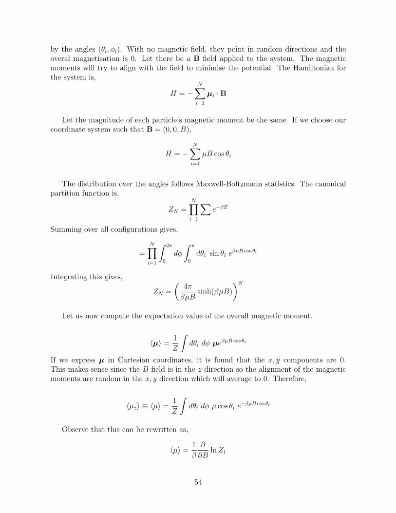
by the angles (θi, φi). With no magnetic field, they point in random directions and theoveral magnetisation is 0. Let there be a B field applied to the system. The magneticmoments will try to align with the field to minimise the potential. The Hamiltonian forthe system is,

H = −N∑i=1

µi ·B

Let the magnitude of each particle’s magnetic moment be the same. If we choose ourcoordinate system such that B = (0, 0, B),

H = −N∑i=1

µB cos θi

The distribution over the angles follows Maxwell-Boltzmann statistics. The canonicalpartition function is,

ZN =N∏i=1

∑e−βE

Summing over all configurations gives,

=N∏i=1

∫ 2π

0

dφ

∫ π

0

dθi sin θi eβµB cos θi

Integrating this gives,

ZN =

(4π

βµBsinh(βµB)

)NLet us now compute the expectation value of the overall magnetic moment.

〈µ〉 =1

Z

∫dθi dφ µeβµB cos θi

If we express µ in Cartesian coordinates, it is found that the x, y components are 0.This makes sense since the B field is in the z direction so the alignment of the magneticmoments are random in the x, y direction which will average to 0. Therefore,

〈µz〉 ≡ 〈µ〉 =1

Z

∫dθi dφ µ cos θi e

−βµB cos θi

Observe that this can be rewritten as,

〈µ〉 =1

β

∂

∂BlnZ1

54

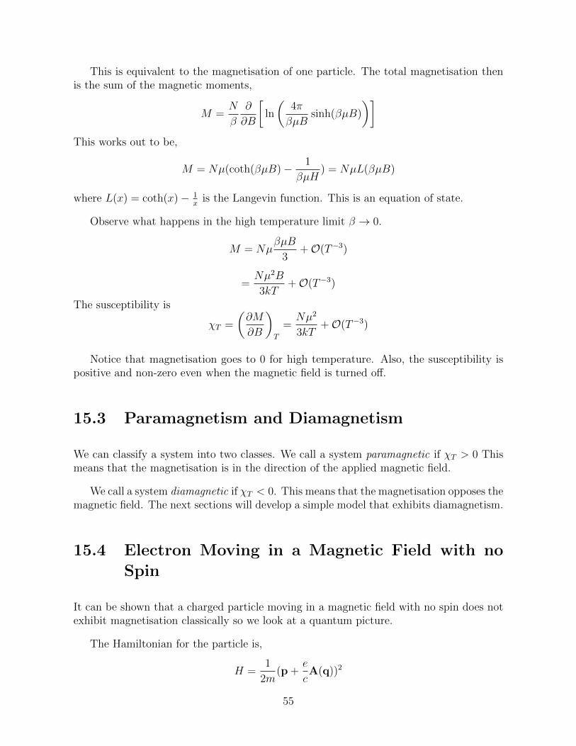
This is equivalent to the magnetisation of one particle. The total magnetisation thenis the sum of the magnetic moments,

M =N

β

∂

∂B

[ln

(4π

βµBsinh(βµB)

)]This works out to be,

M = Nµ(coth(βµB)− 1

βµH) = NµL(βµB)

where L(x) = coth(x)− 1x

is the Langevin function. This is an equation of state.

Observe what happens in the high temperature limit β → 0.

M = NµβµB

3+O(T−3)

=Nµ2B

3kT+O(T−3)

The susceptibility is

χT =

(∂M

∂B

)T

=Nµ2

3kT+O(T−3)

Notice that magnetisation goes to 0 for high temperature. Also, the susceptibility ispositive and non-zero even when the magnetic field is turned off.

15.3 Paramagnetism and Diamagnetism

We can classify a system into two classes. We call a system paramagnetic if χT > 0 Thismeans that the magnetisation is in the direction of the applied magnetic field.

We call a system diamagnetic if χT < 0. This means that the magnetisation opposes themagnetic field. The next sections will develop a simple model that exhibits diamagnetism.

15.4 Electron Moving in a Magnetic Field with no

Spin

It can be shown that a charged particle moving in a magnetic field with no spin does notexhibit magnetisation classically so we look at a quantum picture.

The Hamiltonian for the particle is,

H =1

2m(p +

e

cA(q))2

55

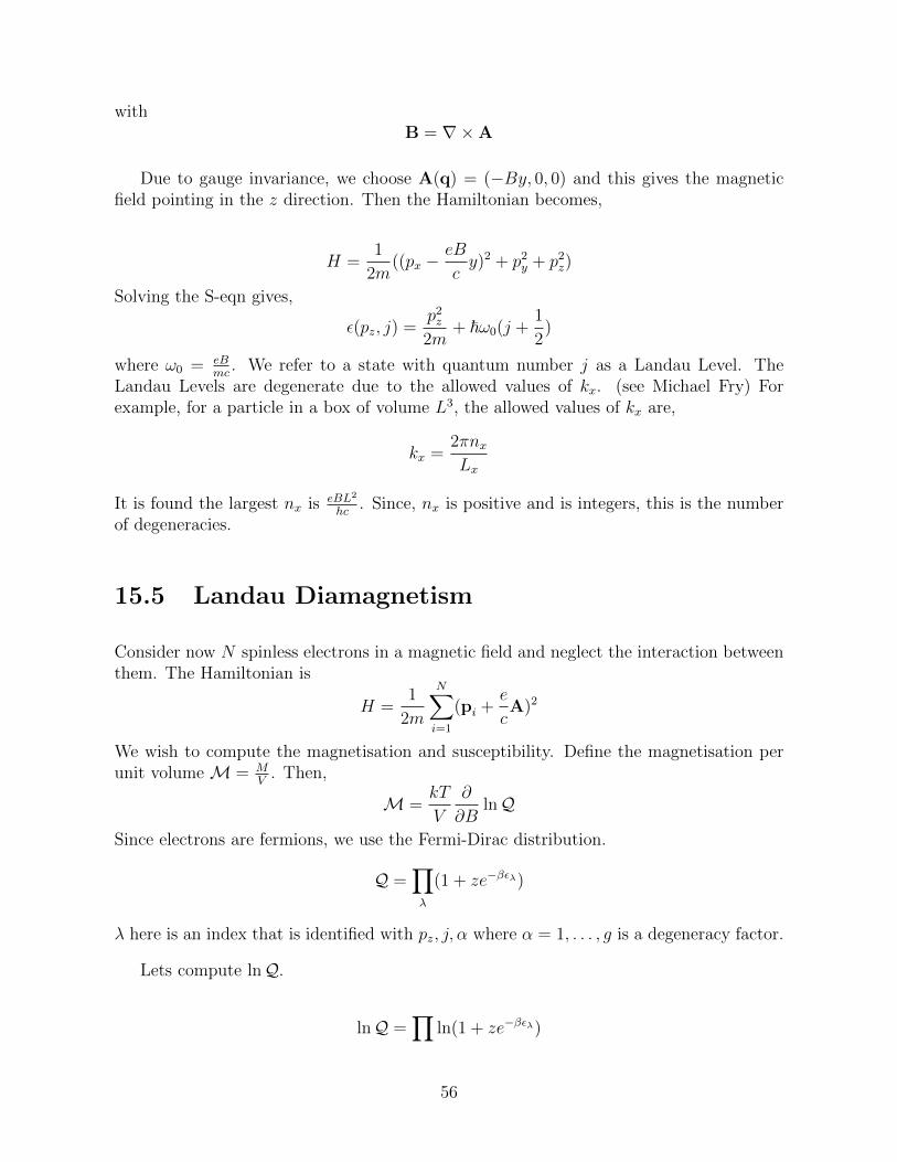
withB = ∇×A

Due to gauge invariance, we choose A(q) = (−By, 0, 0) and this gives the magneticfield pointing in the z direction. Then the Hamiltonian becomes,

H =1

2m((px −

eB

cy)2 + p2

y + p2z)

Solving the S-eqn gives,

ε(pz, j) =p2z

2m+ ~ω0(j +

1

2)

where ω0 = eBmc

. We refer to a state with quantum number j as a Landau Level. TheLandau Levels are degenerate due to the allowed values of kx. (see Michael Fry) Forexample, for a particle in a box of volume L3, the allowed values of kx are,

kx =2πnxLx

It is found the largest nx is eBL2

hc. Since, nx is positive and is integers, this is the number

of degeneracies.

15.5 Landau Diamagnetism

Consider now N spinless electrons in a magnetic field and neglect the interaction betweenthem. The Hamiltonian is

H =1

2m

N∑i=1

(pi +e

cA)2

We wish to compute the magnetisation and susceptibility. Define the magnetisation perunit volume M = M

V. Then,

M =kT

V

∂

∂BlnQ

Since electrons are fermions, we use the Fermi-Dirac distribution.

Q =∏λ

(1 + ze−βελ)

λ here is an index that is identified with pz, j, α where α = 1, . . . , g is a degeneracy factor.

Lets compute lnQ.

lnQ =∏

ln(1 + ze−βελ)

56

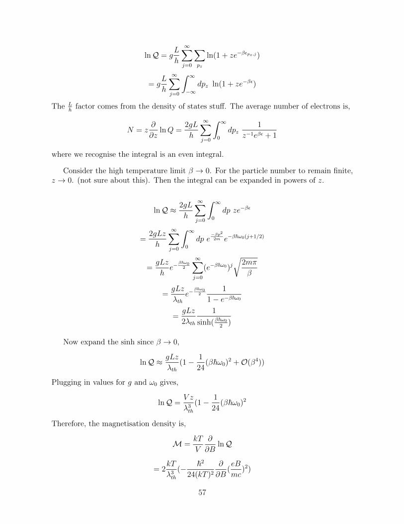
lnQ = gL

h

∞∑j=0

∑pz

ln(1 + ze−βεpz,j)

= gL

h

∞∑j=0

∫ ∞−∞

dpz ln(1 + ze−βε)

The Lh

factor comes from the density of states stuff. The average number of electrons is,

N = z∂

∂zlnQ =

2gL

h

∞∑j=0

∫ ∞0

dpz1

z−1eβε + 1

where we recognise the integral is an even integral.

Consider the high temperature limit β → 0. For the particle number to remain finite,z → 0. (not sure about this). Then the integral can be expanded in powers of z.

lnQ ≈ 2gL

h

∞∑j=0

∫ ∞0

dp ze−βε

=2gLz

h

∞∑j=0

∫ ∞0

dp e−βp22m e−β~ω0(j+1/2)

=gLz

he−

β~ω02

∞∑j=0

(e−β~ω0)j√

2mπ

β

=gLz

λthe−

β~ω02

1

1− e−β~ω0

=gLz

2λth

1

sinh(β~ω0

2)

Now expand the sinh since β → 0,

lnQ ≈ gLz

λth(1− 1

24(β~ω0)2 +O(β4))

Plugging in values for g and ω0 gives,

lnQ =V z

λ3th

(1− 1

24(β~ω0)2

Therefore, the magnetisation density is,

M =kT

V

∂

∂BlnQ

= 2kT

λ3th

(− ~2

24(kT )2

∂

∂B(eB

mc)2)

57

= − 2z

24λ3thkT

(e~mc

)2B

So the susceptibility density is,

χTV

=∂M∂B

=−z

3kTλ3(e~

2mc)2

This is an example of a diamagnetic system which has a negative susceptibility. What’sessentially happening is that the magnetic field causes circular orbits and according toLenz’s Law, an opposing magnetic field must be created.

15.6 De Haas-Van Alphen Effect

Consider the low temperature limit of Landau diamagnetism where the system approachesits ground state. We also assume that motion only occurs in the xy plane. The energycan be rewritten to be

εj = 2µBB(j +1

2)

where µB = e~2mc

is the Bohr magneton.

Rewrite the degeneracy as

g = NB

B0

where B0 = NhcL2e

.

If B ≥ B0, then g ≥ N so all the particles can fit into the ground state. The energy ofthe ground state is E0 = NµBB.

However, if B < B0, then some particles are forced into the next state by the Pauliexclusion principle. Suppose B < B0 and the levels j and below are filled and the levelj + 1 is partly filled and all higher levels are empty. Then (not sure about this)

(j + 1)g < N < (j + 2)g

⇒ 1

j + 2<

B

B0

<1

j + 1

The energy of the system is,

E = g

j∑i=1

εi + (N − (j + 1)g)εj+1

where N − (j + 1)g is the number of remaining particles. This gives,

E = NµBBx(2j + 3− (j + 1)(j + 2)x)

58

where x = BB0

.

To summarise, the energy per particle of the system is,

E

N=

µBBx if x > 1

µBBx(2j + 3− (j + 1)(j + 2)x) if 1j+2

< x < 1j+1

The magnetisation per unit area M = −1L2

∂∂BE is

M =

−NµBL2 if x > 1

µBBx(2j + 3− (j + 1)(j + 2)x) if 1j+2

< x < 1j+1

Something is really wrong so stop here.

59

Chapter 16

Ferromagnetism

We now look at a different class of magnets called ferromagnets. These are magnets thathave magnetisation even when not in the presence of a magnetic field. It is due to theelectron’s spin. It is energetically favoured to have parallel spin. In this model, we assumethat the spins can either point in the positive or negative direction in the z direction(iewe measure Sz, for convenience the z is dropped). Consider a system of N particles. TheHeisenberg model has the Hamiltonian

H = −1

2

∑i,j

JijSiSj − gµBN∑i=1

Si ·B

where B is the magnetic feld, S is the spin of the particle, g is the g-factor. Jij = Jij > 0is a term that measures the interaction between the spins of neighbouring particles. Thereis −J energy for parallel spins and J energy for antiparallel spins.

Firstly, lets develop a bit of the framework we will be using later. The spins followthe usual commutator relations for spin and the spin for the i and j particle commute.This means we can find a simultaenous diagonalised eigenstate for all the particles. Thepartition function looks like

Z = Tr(e−βH) =∑

m1=± 12

· · ·∑

mN=± 12

〈ψm1...mN |e−βH |ψm1...mN 〉

We also have the Gibbs potential energy to be

G(T,B) = −kT lnZ

The expectation value of the energy is,

〈H〉 =1

ZTr(He−βH)

60

= − ∂

∂ββG(T,B)

The magnetiation is

Mα = gµB〈N∑j=1

Sαj 〉

=1

ZTr(gµB

N∑j=1

Sαi e−βH)

=1

βZTr(

∂

∂Bαe−βH) =

1

β

∂

∂BαlnZ

α labels the coordinate x, y, z.

16.1 Non-Interacting Case

Lets now consider the case where J = 0 so the spins do not interact with each other.However, the spins interact with the magnetic field. Choose the coordinate system so thatB points in the z-direction. Then the Hamiltonian is

H = −gµBBN∑i=1

Szi

Therefore, the partition function is,

Z =∑

m1=± 12

· · ·∑

mN=± 12

〈ψm1...mN |eβgµBB∑Szi |ψm1...mN 〉

=∑

m1=± 12

· · ·∑

mN=± 12

eβgµBB∑mi〈ψm1...mN |ψm1...mN 〉

=∑

m1=± 12

· · ·∑

mN=± 12

eβgµBB∑mi

=

( ∑m=± 1

2

eβgµBBm)N

= (e12βgµBB + e−

12βgµBB)N

= 2N coshN(βgµBB

2)

Therefore the magnetisation is,

M = kT∂

∂BlnZ = M0 tanh

βgµBB

2

where M0 = NgµB2

.

61

16.2 Mean Field Approximation

In the mean field approximation, we assume that the spin has the form,

Si = 〈Si〉+ ∆Si

We treat ∆Si as a small approximation. So,

Si · Sj = 〈Si〉〈Sj〉+ ∆Si〈Sj〉+ ∆Sj〈Si〉+O(∆S2)

The Hamiltonian becomes,

H = −1

2

∑i 6=j

Jij

[〈Si〉〈S〉+ 2∆S〈Sj〉

]− gµB

∑Si ·B

= −∑

Jij

[〈Si〉(Sj − 〈Sj〉) +

1

2〈Si〉〈Sj〉

]− gµB

∑Si ·B

62