Speed of a wave v STATE VARIABLE. Energy of a photon E photon STATE VARIABLE.
Upload
haymanotyehualaCategory
view
21download
0
ME 381
Mechanical and Aerospace Control Systems
Dr. Robert G. Landers
State Equation Solution
Unforced Response 2State Equation Solution Dr. Robert G. Landers
( ) ( )t t=x Ax
( ) ( )0tt e= Ax x
( )tt
d ee
dt=
AAA
( ) ( ) ( ) ( )0 0t tt t e e= ⇒ =A Ax Ax A x A x
( ) ( ) ( )0t t=x Φ x
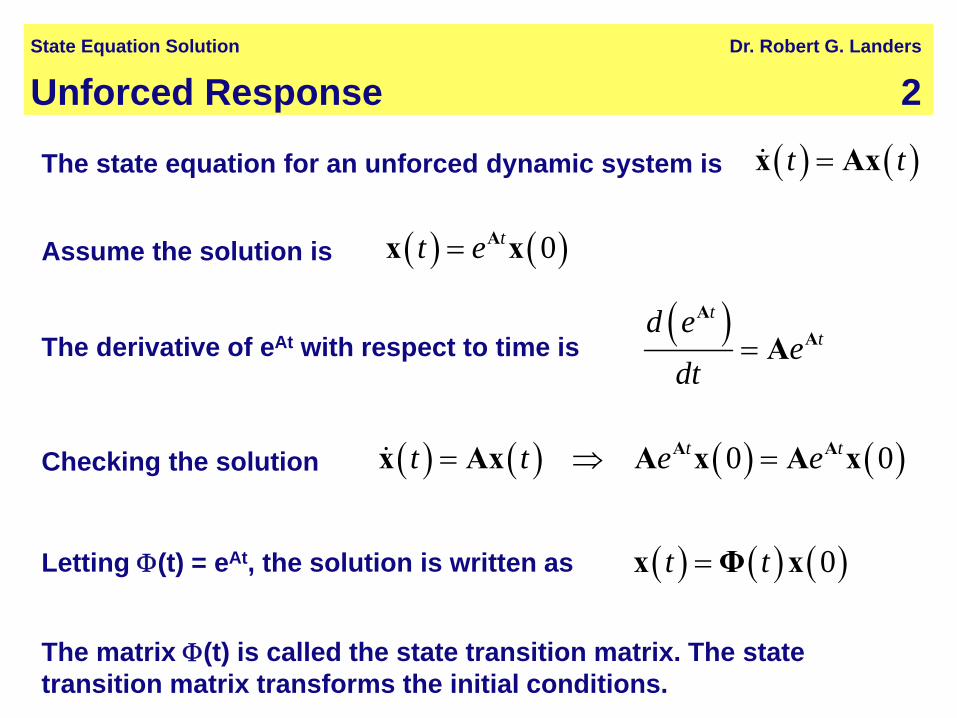
The matrix Φ(t) is called the state transition matrix. The state transition matrix transforms the initial conditions.
The state equation for an unforced dynamic system is
Assume the solution is
The derivative of eAt with respect to time is
Checking the solution
Letting Φ(t) = eAt, the solution is written as
Properties of State Transition Matrices 3
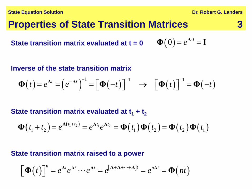
( ) 00 e= =AΦ I
( ) ( ) ( ) ( ) ( )1 1 1t tt e e t t t− − −−= = = − → = −⎡ ⎤ ⎡ ⎤⎣ ⎦ ⎣ ⎦
A AΦ Φ Φ Φ
( ) ( ) ( ) ( ) ( ) ( )1 2 1 21 2 1 2 2 1
t t t tt t e e e t t t t++ = = = =A A AΦ Φ Φ Φ Φ
( ) [ ] ( )n tt t t n tt e e e e e nt+ + += = = =⎡ ⎤⎣ ⎦A A AA A A AΦ Φ
State Equation Solution Dr. Robert G. Landers
State transition matrix evaluated at t = 0
Inverse of the state transition matrix
State transition matrix evaluated at t1 + t2
State transition matrix raised to a power
Forced Response 4
( ) ( ) ( )t t t= +x Ax Bu
( ) ( ) ( )t t t− =x Ax Bu
( ) ( ) ( ) ( )t t tde t t e t e tdt
− − −⎡ ⎤− = =⎡ ⎤⎣ ⎦ ⎣ ⎦A A Ax Ax x Bu
( ) ( )t
te e d
λλ λ
λ ττ
λ λ λ=− −
=⎡ ⎤ =⎣ ⎦ ∫A Ax Bu
State Equation Solution Dr. Robert G. Landers
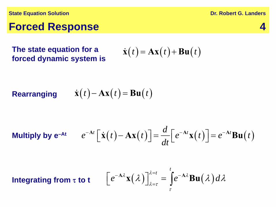
The state equation for a forced dynamic system is
Rearranging
Multiply by e–At
Integrating from τ to t
Forced Response 5
( ) ( ) ( ) ( ) ( )free response
forced response
tt tt e e dτ λ
τ
τ λ λ− −= + ∫A Ax x Bu
( ) ( ) ( ) ( ) ( ) ( )t
t tt t e e dτ λ
τ
τ λ λ− −= = + ∫A Ay Cx C x C Bu
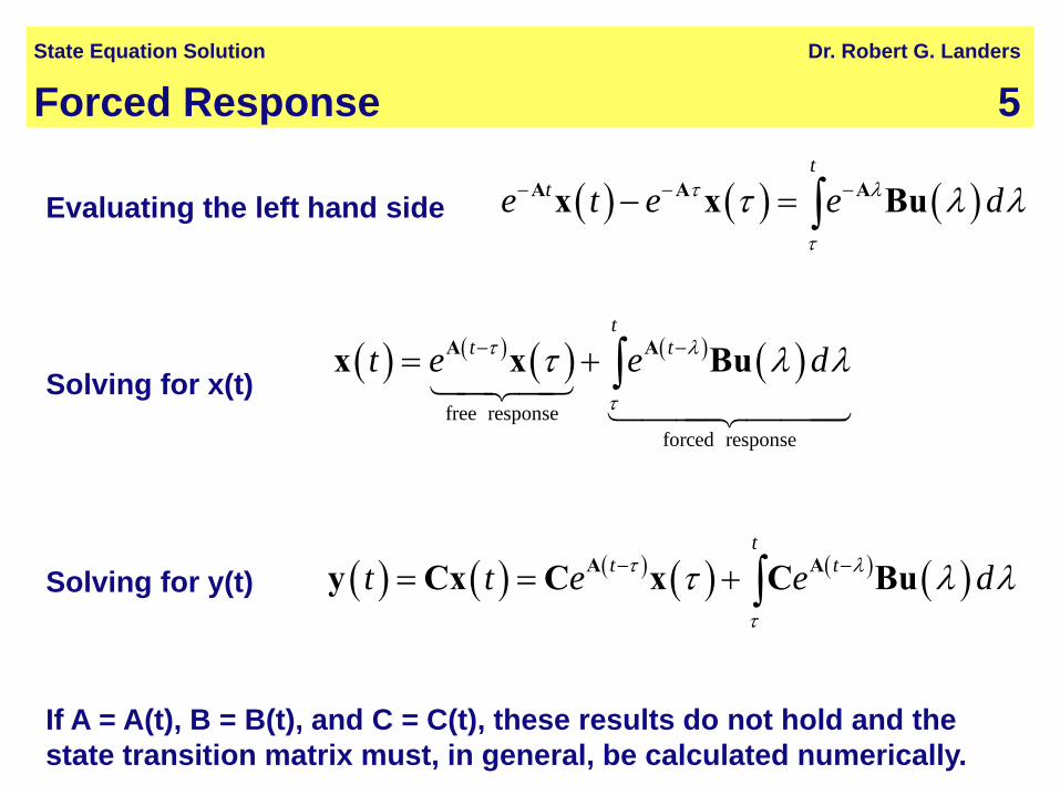
If A = A(t), B = B(t), and C = C(t), these results do not hold and the state transition matrix must, in general, be calculated numerically.
State Equation Solution Dr. Robert G. Landers
Solving for x(t)
Solving for y(t)
( ) ( ) ( )t
te t e e dτ λ
τ
τ λ λ− − −− = ∫A A Ax x BuEvaluating the left hand side
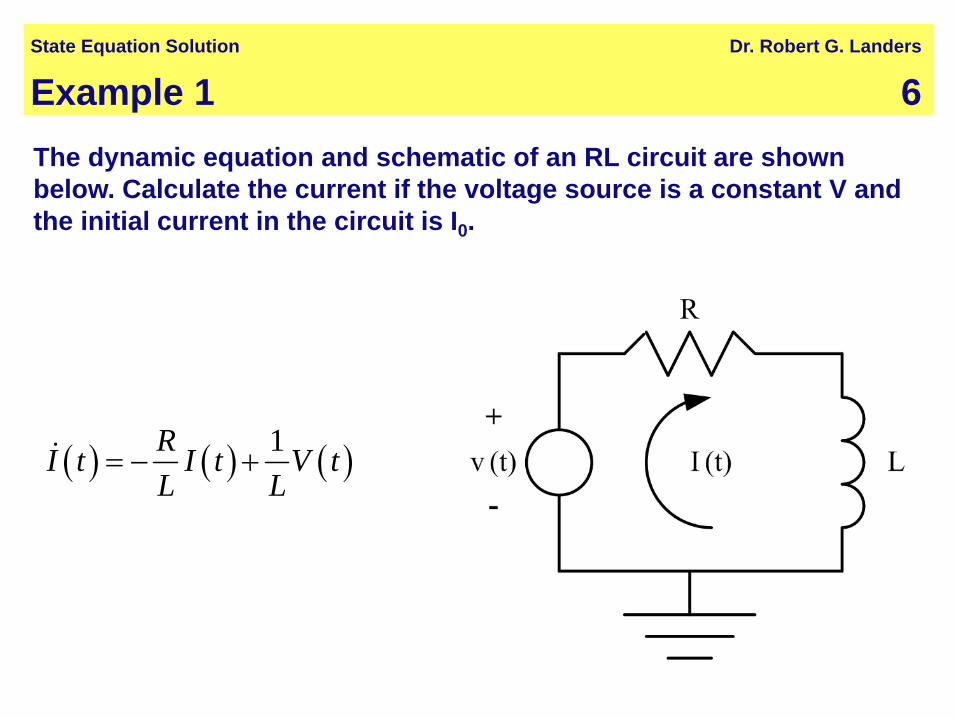
Example 1 6The dynamic equation and schematic of an RL circuit are shown below. Calculate the current if the voltage source is a constant V and the initial current in the circuit is I0.
( ) ( ) ( )1RI t I t V tL L
= − +
State Equation Solution Dr. Robert G. Landers
Example 1 7
( ) ( ) ( ) ( ) 1tR Rt tL LI t e I e Vd
Lτ λ
τ
τ λ− − − −
= + ∫
( ) ( )0
0
tR Rt tL LL VI t I e e
R L
λλ
λ
=− − −
=
⎡ ⎤= + ⎢ ⎥
⎣ ⎦
( ) 0 1R Rt tL LVI t I e e
R− −⎡ ⎤
= + −⎢ ⎥⎣ ⎦
State Equation Solution Dr. Robert G. Landers
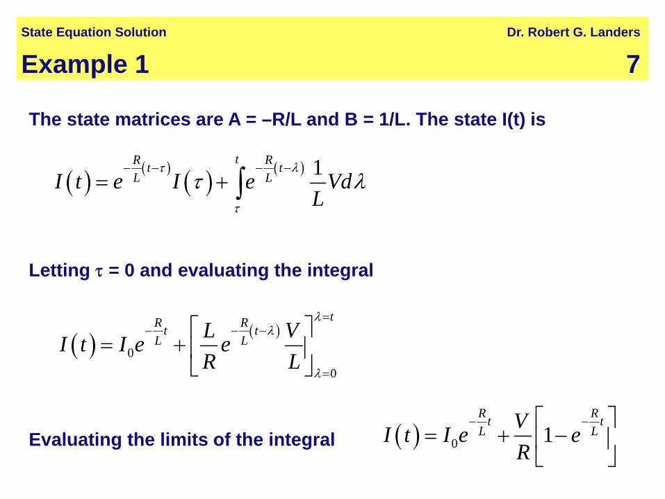
Letting τ = 0 and evaluating the integral
Evaluating the limits of the integral
The state matrices are A = –R/L and B = 1/L. The state I(t) is
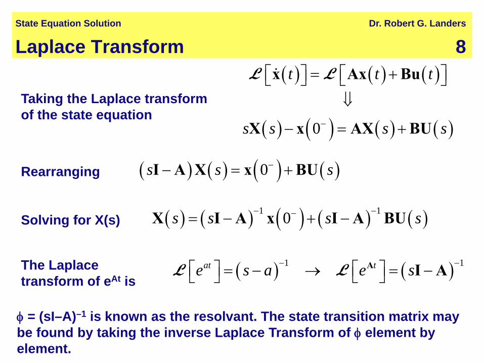
Laplace Transform 8( ) ( ) ( )
( ) ( ) ( ) ( )0
t t t
s s s s−
= +⎡ ⎤ ⎡ ⎤⎣ ⎦ ⎣ ⎦⇓
− = +
x Ax Bu
X x AX BU
L L
( ) ( ) ( ) ( )0s s s−− = +I A X x BU
( ) ( ) ( ) ( ) ( )1 10s s s s− −−= − + −X I A x I A BU
State Equation Solution Dr. Robert G. Landers
Taking the Laplace transform of the state equation
Rearranging
Solving for X(s)
φ = (sI–A)–1 is known as the resolvant. The state transition matrix may be found by taking the inverse Laplace Transform of φ element by element.
The Laplace transform of eAt is ( ) ( )1 1at te s a e s− −⎡ ⎤ ⎡ ⎤= − → = −⎣ ⎦ ⎣ ⎦
A I AL L
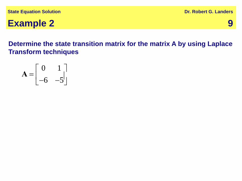
Example 2 9
Determine the state transition matrix for the matrix A by using Laplace Transform techniques
0 16 5
⎡ ⎤= ⎢ ⎥− −⎣ ⎦
A
State Equation Solution Dr. Robert G. Landers
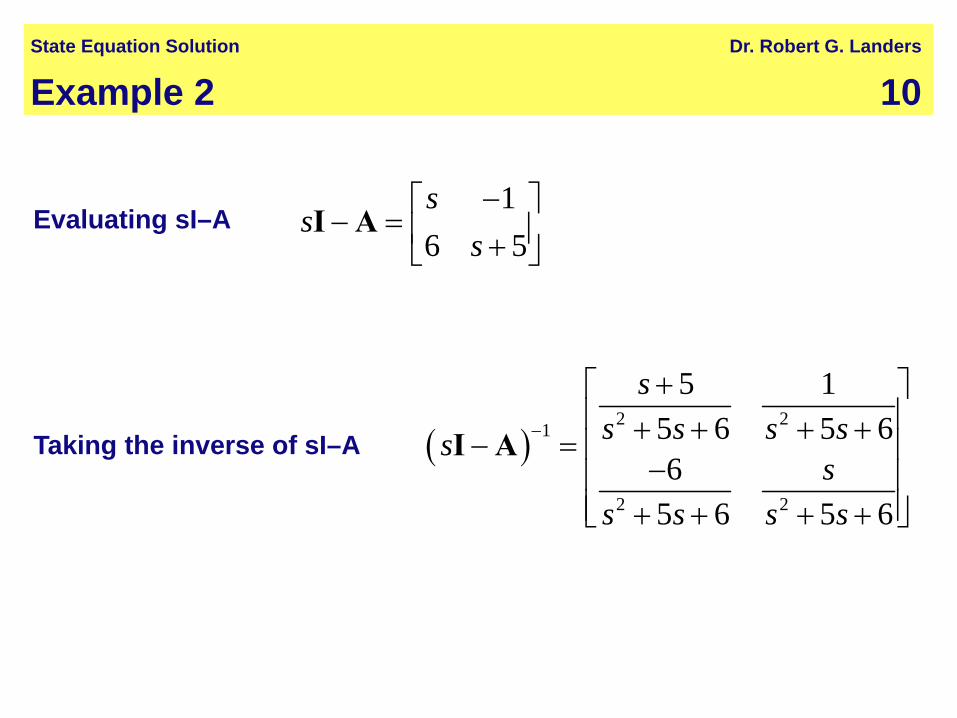
Example 2 10
Evaluating sI–A1
6 5s
ss−⎡ ⎤
− = ⎢ ⎥+⎣ ⎦I A
( )2 21
2 2
5 15 6 5 66
5 6 5 6
ss s s ss
ss s s s
−
+⎡ ⎤⎢ ⎥+ + + +− = ⎢ ⎥
−⎢ ⎥⎢ ⎥+ + + +⎣ ⎦
I A
State Equation Solution Dr. Robert G. Landers
Taking the inverse of sI–A
Example 2 11
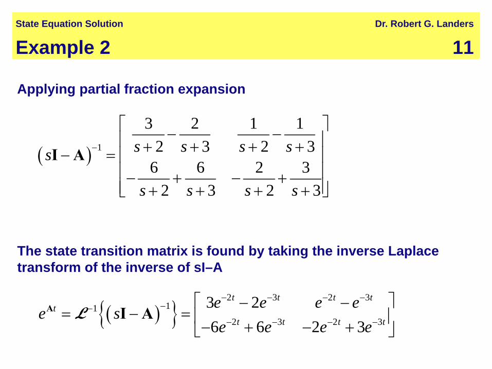
( ){ }2 3 2 3
112 3 2 3
3 26 6 2 3
t t t tt
t t t t
e e e ee s
e e e e
− − − −−−
− − − −
⎡ ⎤− −= − = ⎢ ⎥− + − +⎣ ⎦
A I AL
( ) 1
3 2 1 12 3 2 3
6 6 2 32 3 2 3
s s s ss
s s s s
−
⎡ ⎤− −⎢ ⎥+ + + +− = ⎢ ⎥⎢ ⎥− + − +⎢ ⎥+ + + +⎣ ⎦
I A
State Equation Solution Dr. Robert G. Landers
Applying partial fraction expansion
The state transition matrix is found by taking the inverse Laplace transform of the inverse of sI–A
Transfer Function 12
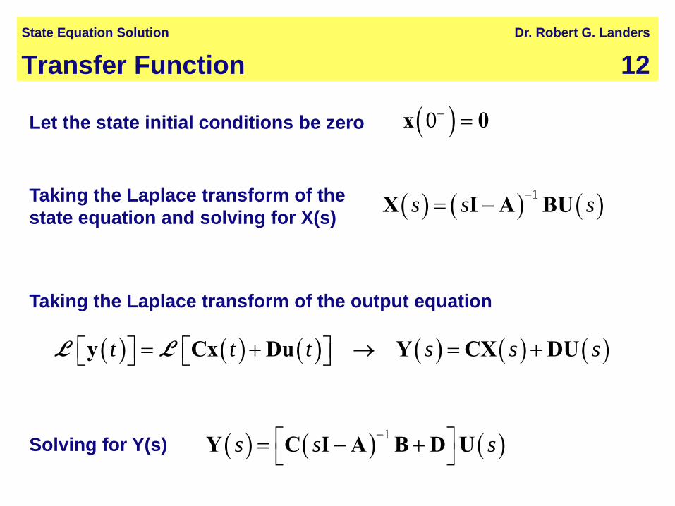
( )0− =x 0
( ) ( ) ( )1s s s−= −X I A BU
( ) ( ) ( ) ( ) ( ) ( )t t t s s s= + → = +⎡ ⎤ ⎡ ⎤⎣ ⎦ ⎣ ⎦y Cx Du Y CX DUL L
( ) ( ) ( )1s s s−⎡ ⎤= − +⎣ ⎦Y C I A B D U
State Equation Solution Dr. Robert G. Landers
Let the state initial conditions be zero
Taking the Laplace transform of the state equation and solving for X(s)
Taking the Laplace transform of the output equation
Solving for Y(s)
Transfer Function 13
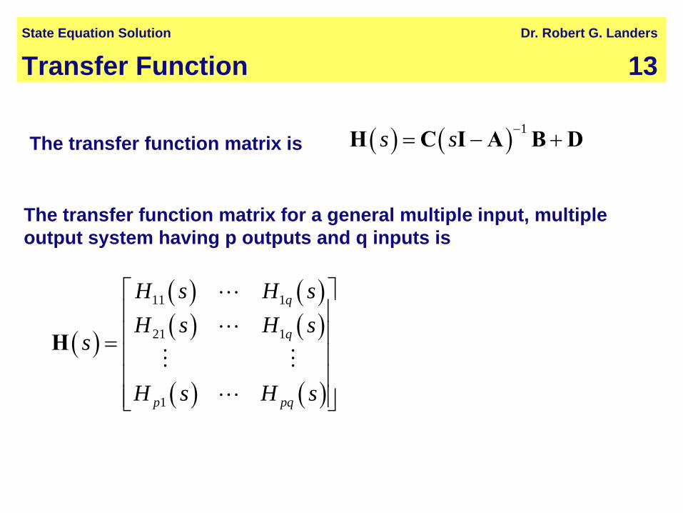
The transfer function matrix for a general multiple input, multiple output system having p outputs and q inputs is
( )
( ) ( )( ) ( )
( ) ( )
11 1
21 1
1
q
q
p pq
H s H sH s H s
s
H s H s
⎡ ⎤⎢ ⎥⎢ ⎥= ⎢ ⎥⎢ ⎥⎢ ⎥⎣ ⎦
H
State Equation Solution Dr. Robert G. Landers
( ) ( ) 1s s −= − +H C I A B DThe transfer function matrix is
Transformation of State Variables 14
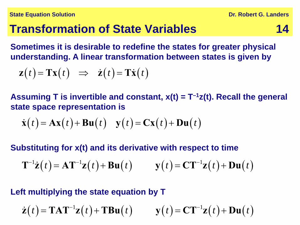
( ) ( ) ( ) ( )t t t t= ⇒ =z Tx z Tx
Sometimes it is desirable to redefine the states for greater physical understanding. A linear transformation between states is given by
Assuming T is invertible and constant, x(t) = T–1z(t). Recall the general state space representation is
( ) ( ) ( ) ( ) ( ) ( )t t t t t t= + = +x Ax Bu y Cx Du
( ) ( ) ( ) ( ) ( ) ( )1 1 1t t t t t t− − −= + = +T z AT z Bu y CT z Du
( ) ( ) ( ) ( ) ( ) ( )1 1t t t t t t− −= + = +z TAT z TBu y CT z Du
State Equation Solution Dr. Robert G. Landers
Substituting for x(t) and its derivative with respect to time
Left multiplying the state equation by T
Transformation of State Variables 15
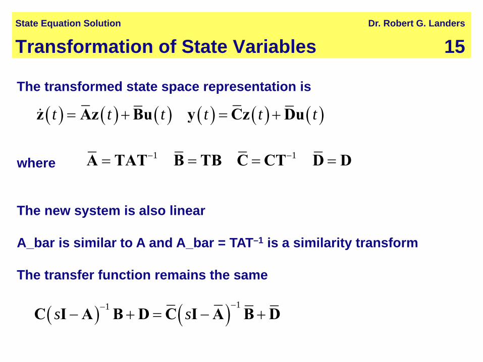
The new system is also linear
A_bar is similar to A and A_bar = TAT–1 is a similarity transform
The transfer function remains the same
1 1− −= = = =A TAT B TB C CT D D
( ) ( ) 11s s−−− + = − +C I A B D C I A B D
State Equation Solution Dr. Robert G. Landers
( ) ( ) ( ) ( ) ( ) ( )t t t t t t= + = +z Az Bu y Cz Du
The transformed state space representation is
where
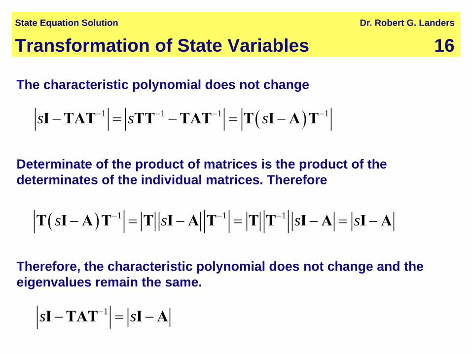
Transformation of State Variables 16
( )1 1 1 1s s s− − − −− = − = −I TAT TT TAT T I A T
The characteristic polynomial does not change
Determinate of the product of matrices is the product of the determinates of the individual matrices. Therefore
( ) 1 1 1s s s s− − −− = − = − = −T I A T T I A T T T I A I A
1s s−− = −I TAT I A
Therefore, the characteristic polynomial does not change and the eigenvalues remain the same.
State Equation Solution Dr. Robert G. Landers
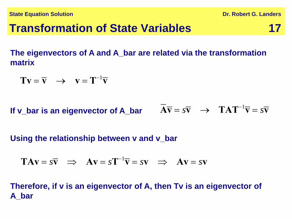
Transformation of State Variables 17
The eigenvectors of A and A_bar are related via the transformation matrix
1−= → =Tv v v T v
1s s−= → =Av v TAT v v
1s s s s−= ⇒ = = ⇒ =TAv v Av T v v Av v
State Equation Solution Dr. Robert G. Landers
Using the relationship between v and v_bar
Therefore, if v is an eigenvector of A, then Tv is an eigenvector of A_bar
If v_bar is an eigenvector of A_bar
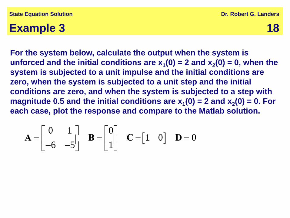
Example 3 18
For the system below, calculate the output when the system is unforced and the initial conditions are x1(0) = 2 and x2(0) = 0, when the system is subjected to a unit impulse and the initial conditions are zero, when the system is subjected to a unit step and the initial conditions are zero, and when the system is subjected to a step with magnitude 0.5 and the initial conditions are x1(0) = 2 and x2(0) = 0. For each case, plot the response and compare to the Matlab solution.
[ ]0 1 01 0 0
6 5 1⎡ ⎤ ⎡ ⎤
= = = =⎢ ⎥ ⎢ ⎥− −⎣ ⎦ ⎣ ⎦A B C D
State Equation Solution Dr. Robert G. Landers
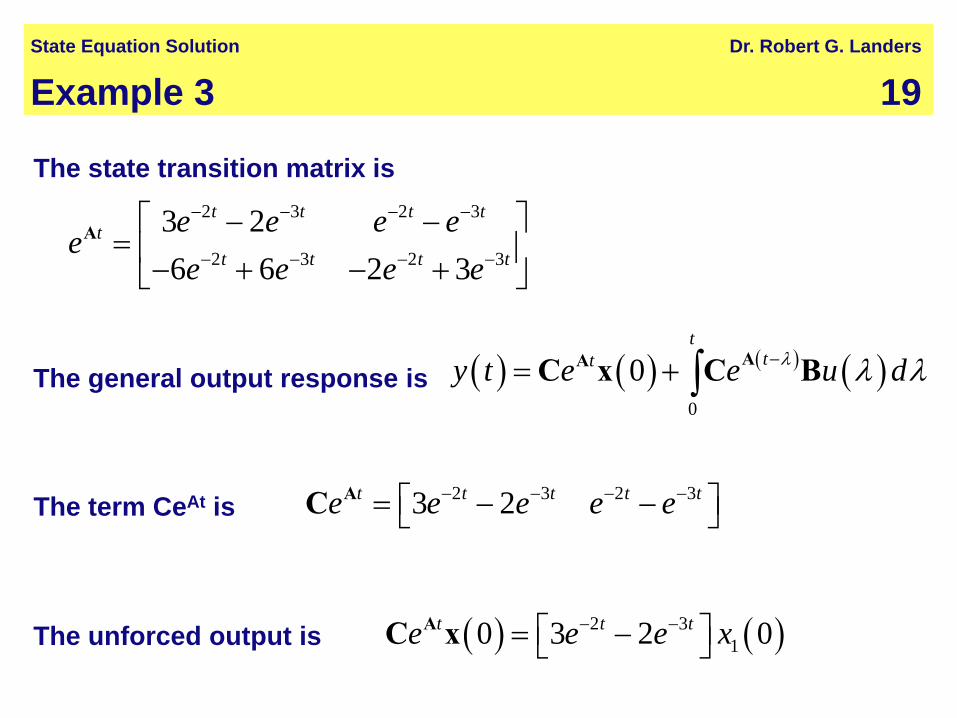
Example 3 19
2 3 2 33 2t t t t te e e e e− − − −⎡ ⎤= − −⎣ ⎦AC
( ) ( ) ( ) ( )0
0t
tty t e e u dλ λ λ−= + ∫ AAC x C BThe general output response is
( ) ( )2 310 3 2 0t t te e e x− −⎡ ⎤= −⎣ ⎦
AC xThe unforced output is
State Equation Solution Dr. Robert G. Landers
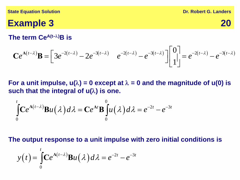
The term CeAt is
The state transition matrix is2 3 2 3
2 3 2 3
3 26 6 2 3
t t t tt
t t t t
e e e ee
e e e e
− − − −
− − − −
⎡ ⎤− −= ⎢ ⎥− + − +⎣ ⎦
A
Example 3 20
For a unit impulse, u(λ) = 0 except at λ = 0 and the magnitude of u(0) is such that the integral of u(λ) is one.
( ) ( ) ( )0
2 3
0 0
tt t t te u d e u d e eλ λ λ λ λ− − −= = −∫ ∫A AC B C B
( ) ( ) ( ) ( ) ( ) ( ) ( )2 3 2 3 2 303 2
1t t t t t t te e e e e e eλ λ λ λ λ λ λ− − − − − − − − − − − − −⎡ ⎤⎡ ⎤= − − = −⎢ ⎥⎣ ⎦ ⎣ ⎦
AC B
The output response to a unit impulse with zero initial conditions is
( ) ( ) ( ) 2 3
0
tt t ty t e u d e eλ λ λ− − −= = −∫ AC B
State Equation Solution Dr. Robert G. Landers
The term CeA(t–λ)B is
Example 3 21
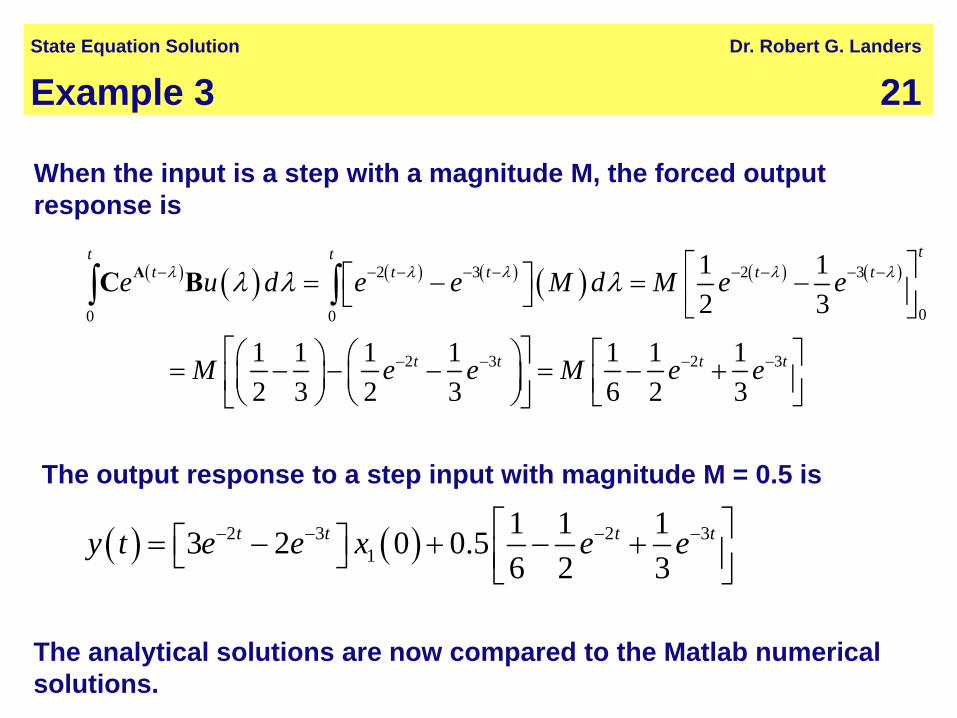
( ) ( )2 3 2 31
1 1 13 2 0 0.56 2 3
t t t ty t e e x e e− − − −⎡ ⎤⎡ ⎤= − + − +⎣ ⎦ ⎢ ⎥⎣ ⎦
The output response to a step input with magnitude M = 0.5 is
( ) ( ) ( ) ( ) ( ) ( ) ( )2 3 2 3
00 0
2 3 2 3
1 12 3
1 1 1 1 1 1 12 3 2 3 6 2 3
tt tt t t t t
t t t t
e u d e e M d M e e
M e e M e e
λ λ λ λ λλ λ λ− − − − − − − − −
− − − −
⎡ ⎤⎡ ⎤= − = −⎢ ⎥⎣ ⎦ ⎣ ⎦
⎡ ⎤⎛ ⎞ ⎛ ⎞ ⎡ ⎤= − − − = − +⎜ ⎟ ⎜ ⎟⎢ ⎥ ⎢ ⎥⎝ ⎠ ⎝ ⎠ ⎣ ⎦⎣ ⎦
∫ ∫AC B
The analytical solutions are now compared to the Matlab numerical solutions.
State Equation Solution Dr. Robert G. Landers
When the input is a step with a magnitude M, the forced output response is