Chapter 4: Elements of Linear System Theoryeus204/teaching/ME450_MRC/... · 2017-01-11 · Elements...
77
Lecture 3 Chapter 4: Elements of Linear System Theory Eugenio Schuster [email protected] Mechanical Engineering and Mechanics Lehigh University Lecture 3 – p. 1/77
Transcript of Chapter 4: Elements of Linear System Theoryeus204/teaching/ME450_MRC/... · 2017-01-11 · Elements...
Lecture 3
Chapter 4: Elements of Linear System Theory
Eugenio Schuster
Mechanical Engineering and Mechanics
Lehigh University
Lecture 3 – p. 1/77
Elements of Linear System Theory
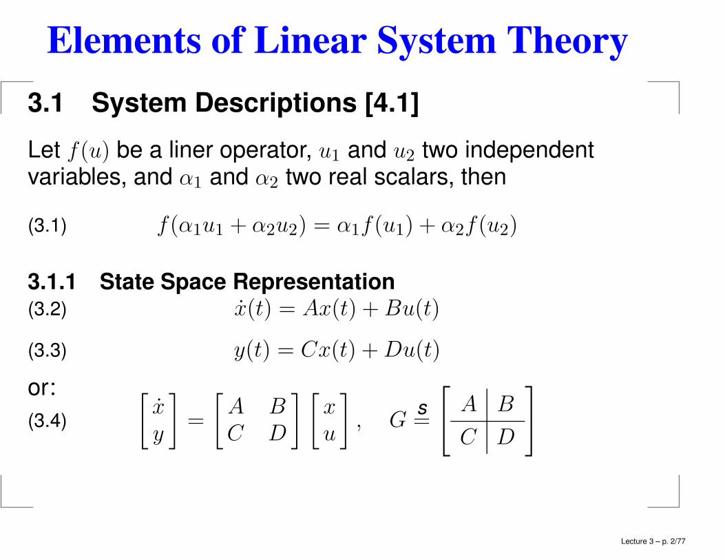
3.1 System Descriptions [4.1]
Let f(u) be a liner operator, u1 and u2 two independentvariables, and α1 and α2 two real scalars, then
f(α1u1 + α2u2) = α1f(u1) + α2f(u2)(3.1)
3.1.1 State Space Representationx(t) = Ax(t) +Bu(t)(3.2)
y(t) = Cx(t) +Du(t)(3.3)
or: [xy
]=
[A BC D
] [xu
], G
s=
[A B
C D
](3.4)
Lecture 3 – p. 2/77
Elements of Linear System Theory
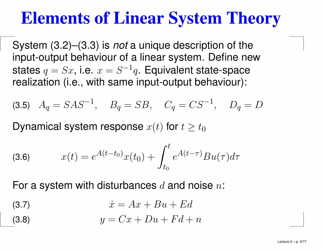
System (3.2)–(3.3) is not a unique description of theinput-output behaviour of a linear system. Define new
states q = Sx, i.e. x = S−1q. Equivalent state-spacerealization (i.e., with same input-output behaviour):
Aq = SAS−1, Bq = SB, Cq = CS−1, Dq = D(3.5)
Dynamical system response x(t) for t ≥ t0
x(t) = eA(t−t0)x(t0) +
∫ t
t0
eA(t−τ)Bu(τ)dτ(3.6)
For a system with disturbances d and noise n:
x = Ax+Bu+ Ed(3.7)
y = Cx+Du+ Fd+ n(3.8)
Lecture 3 – p. 3/77
Elements of Linear System Theory
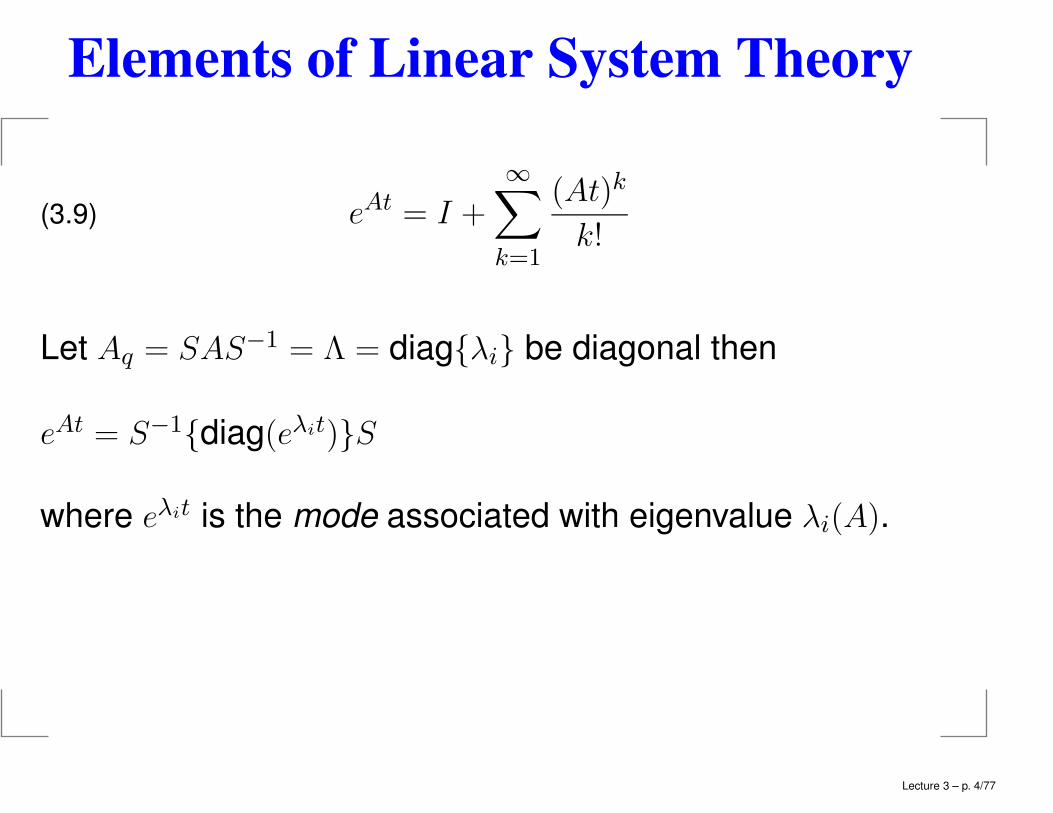
eAt = I +
∞∑
k=1
(At)k
k!(3.9)
Let Aq = SAS−1 = Λ = diag{λi} be diagonal then
eAt = S−1{diag(eλit)}S
where eλit is the mode associated with eigenvalue λi(A).
Lecture 3 – p. 4/77
Elements of Linear System Theory
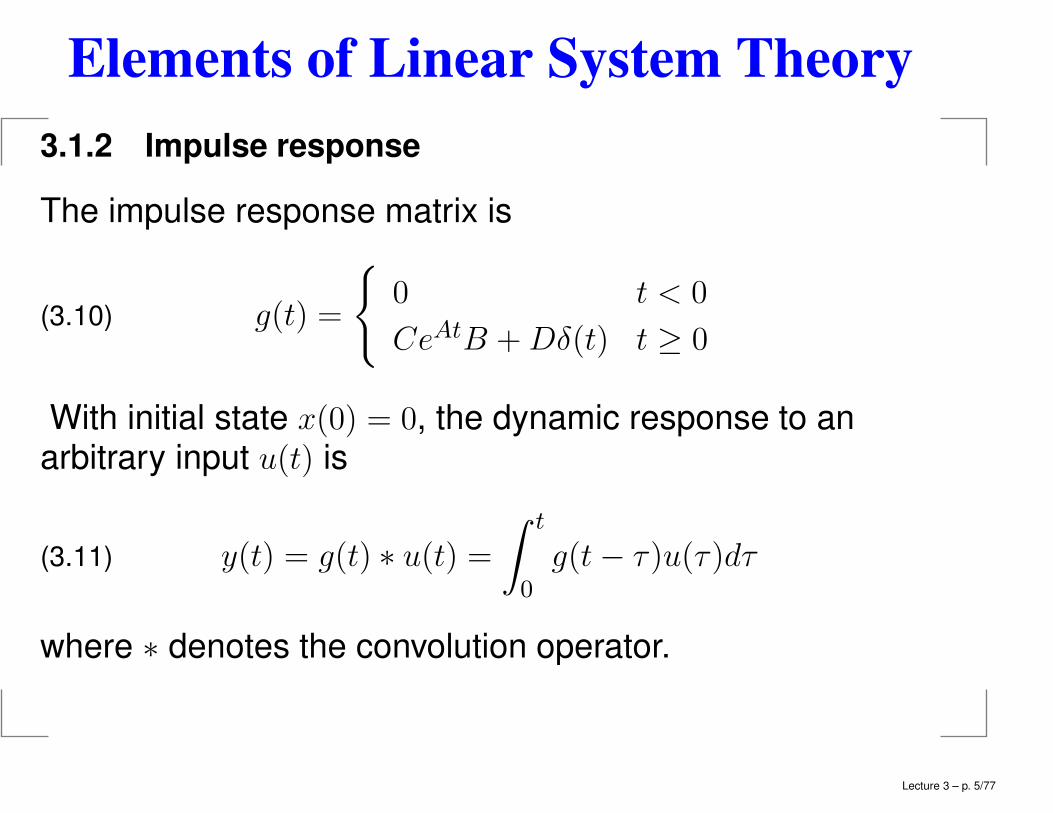
3.1.2 Impulse response
The impulse response matrix is
g(t) =
{0 t < 0
CeAtB +Dδ(t) t ≥ 0(3.10)
With initial state x(0) = 0, the dynamic response to anarbitrary input u(t) is
y(t) = g(t) ∗ u(t) =
∫ t
0
g(t− τ)u(τ)dτ(3.11)
where ∗ denotes the convolution operator.
Lecture 3 – p. 5/77
Elements of Linear System Theory
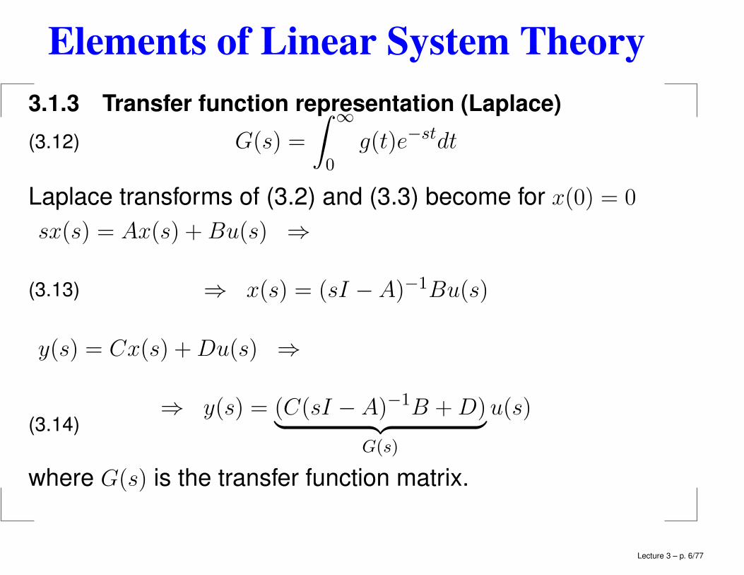
3.1.3 Transfer function representation (Laplace)
G(s) =
∫ ∞
0
g(t)e−stdt(3.12)
Laplace transforms of (3.2) and (3.3) become for x(0) = 0
sx(s) = Ax(s) + Bu(s) ⇒
⇒ x(s) = (sI −A)−1Bu(s)(3.13)
y(s) = Cx(s) +Du(s) ⇒
⇒ y(s) = (C(sI − A)−1B +D)︸ ︷︷ ︸G(s)
u(s)(3.14)
where G(s) is the transfer function matrix.
Lecture 3 – p. 6/77
Elements of Linear System Theory
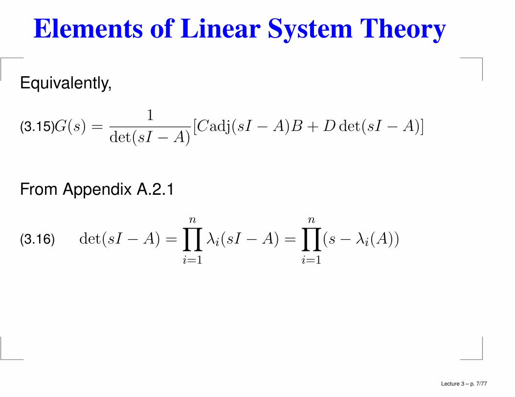
Equivalently,
G(s) =1
det(sI −A)[Cadj(sI − A)B +D det(sI −A)](3.15)
From Appendix A.2.1
det(sI − A) =
n∏
i=1
λi(sI − A) =
n∏
i=1
(s− λi(A))(3.16)
Lecture 3 – p. 7/77
Elements of Linear System Theory
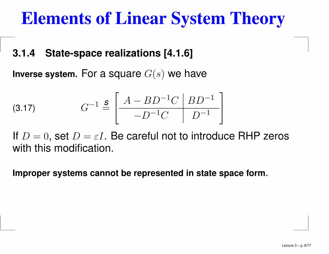
3.1.4 State-space realizations [4.1.6]
Inverse system. For a square G(s) we have
G−1 s=
[A−BD−1C BD−1
−D−1C D−1
](3.17)
If D = 0, set D = εI. Be careful not to introduce RHP zeroswith this modification.
Improper systems cannot be represented in state space form.
Lecture 3 – p. 8/77
Elements of Linear System Theory
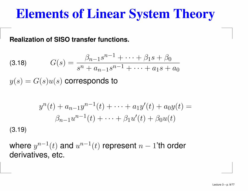
Realization of SISO transfer functions.
G(s) =βn−1s
n−1 + · · · + β1s+ β0sn + an−1sn−1 + · · · + a1s+ a0
(3.18)
y(s) = G(s)u(s) corresponds to
yn(t) + an−1yn−1(t) + · · · + a1y
′(t) + a0y(t) =
βn−1un−1(t) + · · · + β1u
′(t) + β0u(t)
(3.19)
where yn−1(t) and un−1(t) represent n− 1’th orderderivatives, etc.
Lecture 3 – p. 9/77
Elements of Linear System Theory
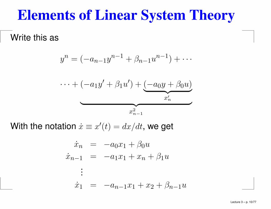
Write this as
yn = (−an−1yn−1 + βn−1u
n−1) + · · ·
· · · + (−a1y′ + β1u
′) + (−a0y + β0u)︸ ︷︷ ︸x′n︸ ︷︷ ︸
x2n−1
With the notation x ≡ x′(t) = dx/dt, we get
xn = −a0x1 + β0u
xn−1 = −a1x1 + xn + β1u
...
x1 = −an−1x1 + x2 + βn−1u
Lecture 3 – p. 10/77
Elements of Linear System Theory
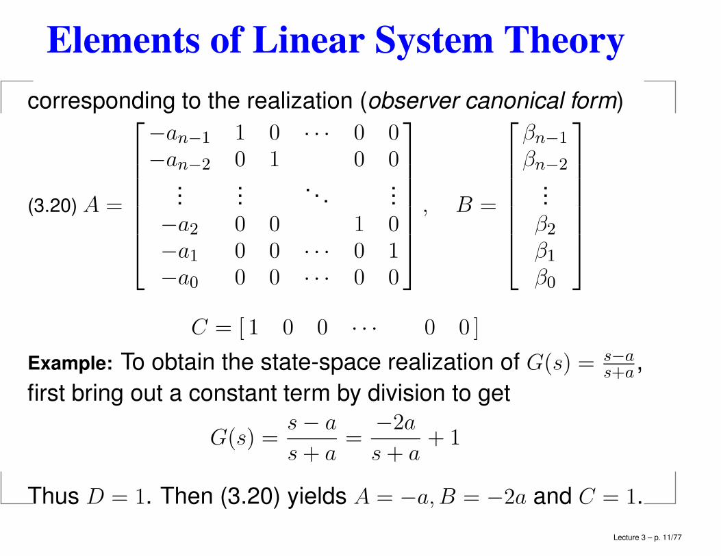
corresponding to the realization (observer canonical form)
A =
−an−1 1 0 · · · 0 0−an−2 0 1 0 0
......
. . ....
−a2 0 0 1 0−a1 0 0 · · · 0 1−a0 0 0 · · · 0 0
, B =
βn−1
βn−2...β2β1β0
(3.20)
C = [ 1 0 0 · · · 0 0 ]
Example: To obtain the state-space realization of G(s) = s−as+a ,
first bring out a constant term by division to get
G(s) =s− a
s+ a=
−2a
s+ a+ 1
Thus D = 1. Then (3.20) yields A = −a,B = −2a and C = 1.
Lecture 3 – p. 11/77
Elements of Linear System Theory
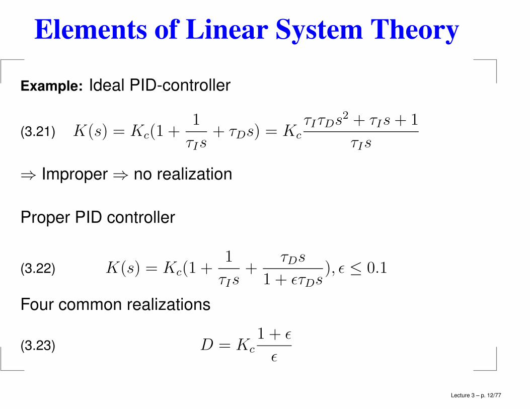
Example: Ideal PID-controller
K(s) = Kc(1 +1
τIs+ τDs) = Kc
τIτDs2 + τIs+ 1
τIs(3.21)
⇒ Improper ⇒ no realization
Proper PID controller
K(s) = Kc(1 +1
τIs+
τDs
1 + ǫτDs), ǫ ≤ 0.1(3.22)
Four common realizations
D = Kc
1 + ǫ
ǫ(3.23)
Lecture 3 – p. 12/77
Elements of Linear System Theory
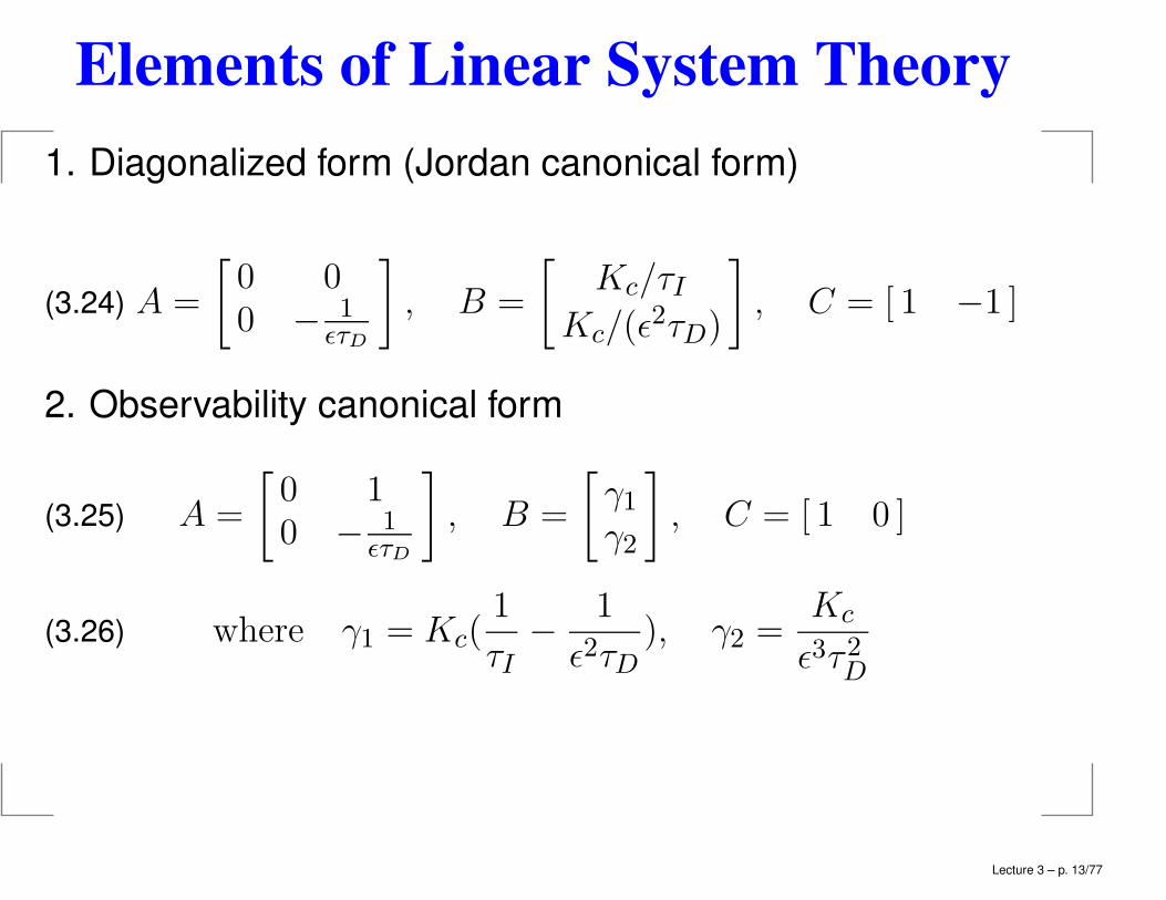
1. Diagonalized form (Jordan canonical form)
A =
[0 00 − 1
ǫτD
], B =
[Kc/τI
Kc/(ǫ2τD)
], C = [ 1 −1 ](3.24)
2. Observability canonical form
A =
[0 10 − 1
ǫτD
], B =
[γ1γ2
], C = [ 1 0 ](3.25)
where γ1 = Kc(1
τI−
1
ǫ2τD), γ2 =
Kc
ǫ3τ2D(3.26)
Lecture 3 – p. 13/77
Elements of Linear System Theory
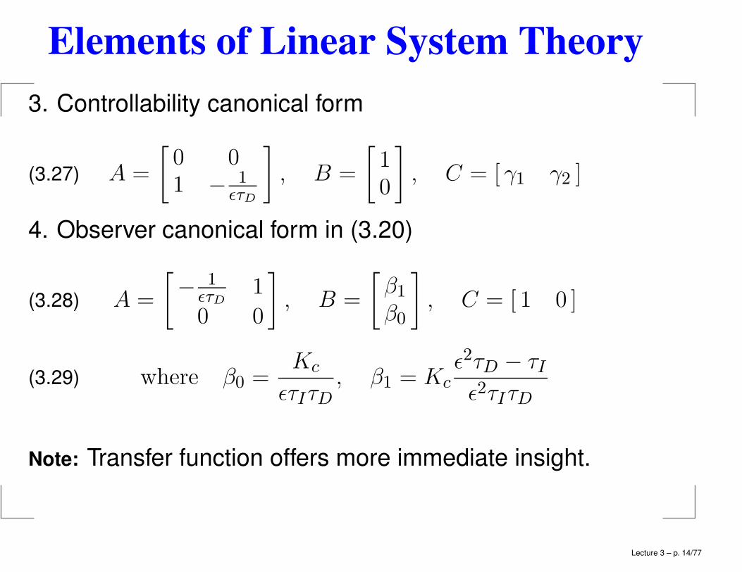
3. Controllability canonical form
A =
[0 01 − 1
ǫτD
], B =
[10
], C = [ γ1 γ2 ](3.27)
4. Observer canonical form in (3.20)
A =
[− 1
ǫτD1
0 0
], B =
[β1β0
], C = [ 1 0 ](3.28)
where β0 =Kc
ǫτIτD, β1 = Kc
ǫ2τD − τIǫ2τIτD
(3.29)
Note: Transfer function offers more immediate insight.
Lecture 3 – p. 14/77
Elements of Linear System Theory
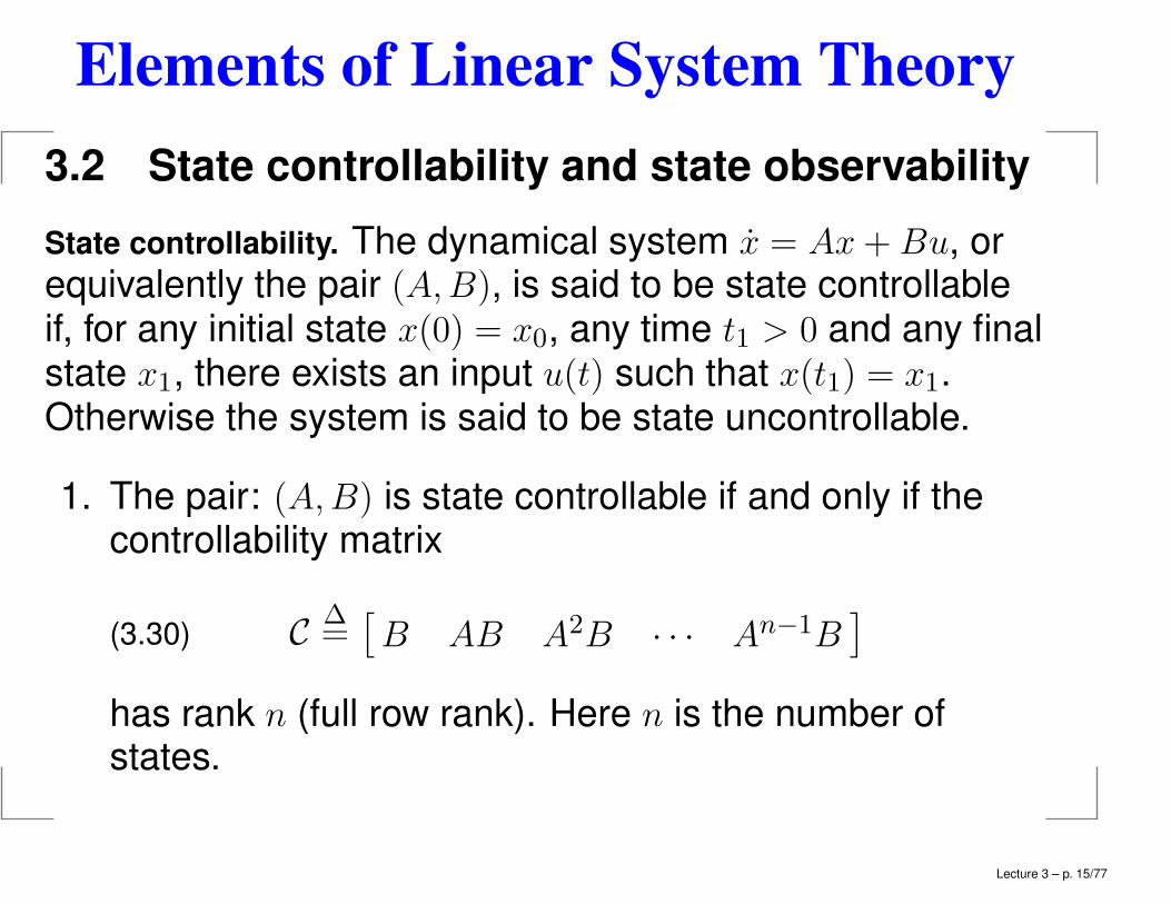
3.2 State controllability and state observability
State controllability. The dynamical system x = Ax+ Bu, orequivalently the pair (A,B), is said to be state controllableif, for any initial state x(0) = x0, any time t1 > 0 and any finalstate x1, there exists an input u(t) such that x(t1) = x1.Otherwise the system is said to be state uncontrollable.
1. The pair: (A,B) is state controllable if and only if thecontrollability matrix
C∆=
[B AB A2B · · · An−1B
](3.30)
has rank n (full row rank). Here n is the number ofstates.
Lecture 3 – p. 15/77
Elements of Linear System Theory
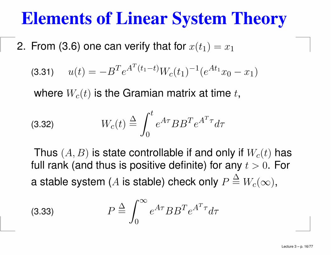
2. From (3.6) one can verify that for x(t1) = x1
u(t) = −BT eAT (t1−t)Wc(t1)
−1(eAt1x0 − x1)(3.31)
where Wc(t) is the Gramian matrix at time t,
Wc(t)∆=
∫ t
0
eAτBBT eAT τdτ(3.32)
Thus (A,B) is state controllable if and only if Wc(t) hasfull rank (and thus is positive definite) for any t > 0. For
a stable system (A is stable) check only P∆= Wc(∞),
P∆=
∫ ∞
0
eAτBBT eAT τdτ(3.33)
Lecture 3 – p. 16/77
Elements of Linear System Theory
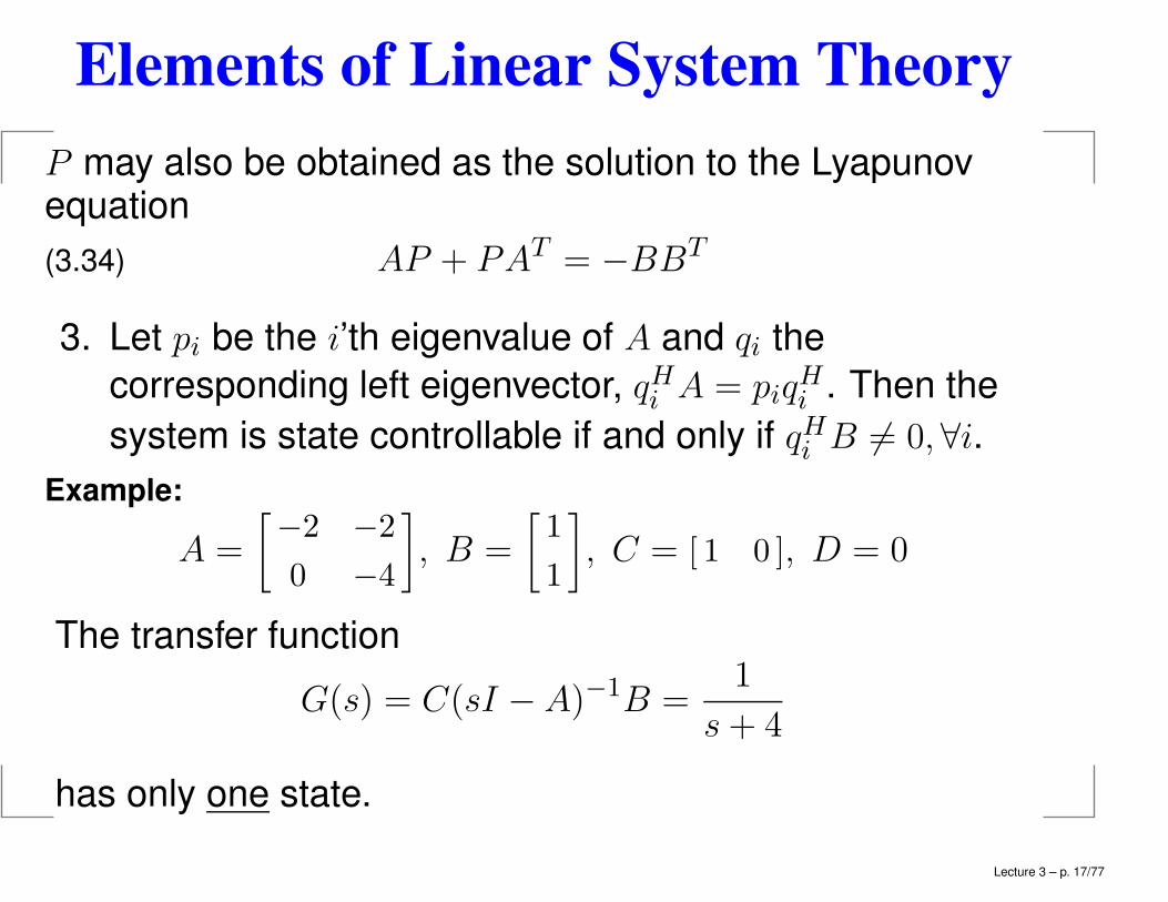
P may also be obtained as the solution to the Lyapunovequation
AP + PAT = −BBT(3.34)
3. Let pi be the i’th eigenvalue of A and qi the
corresponding left eigenvector, qHi A = piqHi . Then the
system is state controllable if and only if qHi B 6= 0,∀i.
Example:
A =
[−2 −2
0 −4
], B =
[1
1
], C = [ 1 0 ], D = 0
The transfer function
G(s) = C(sI −A)−1B =1
s+ 4
has only one state.
Lecture 3 – p. 17/77
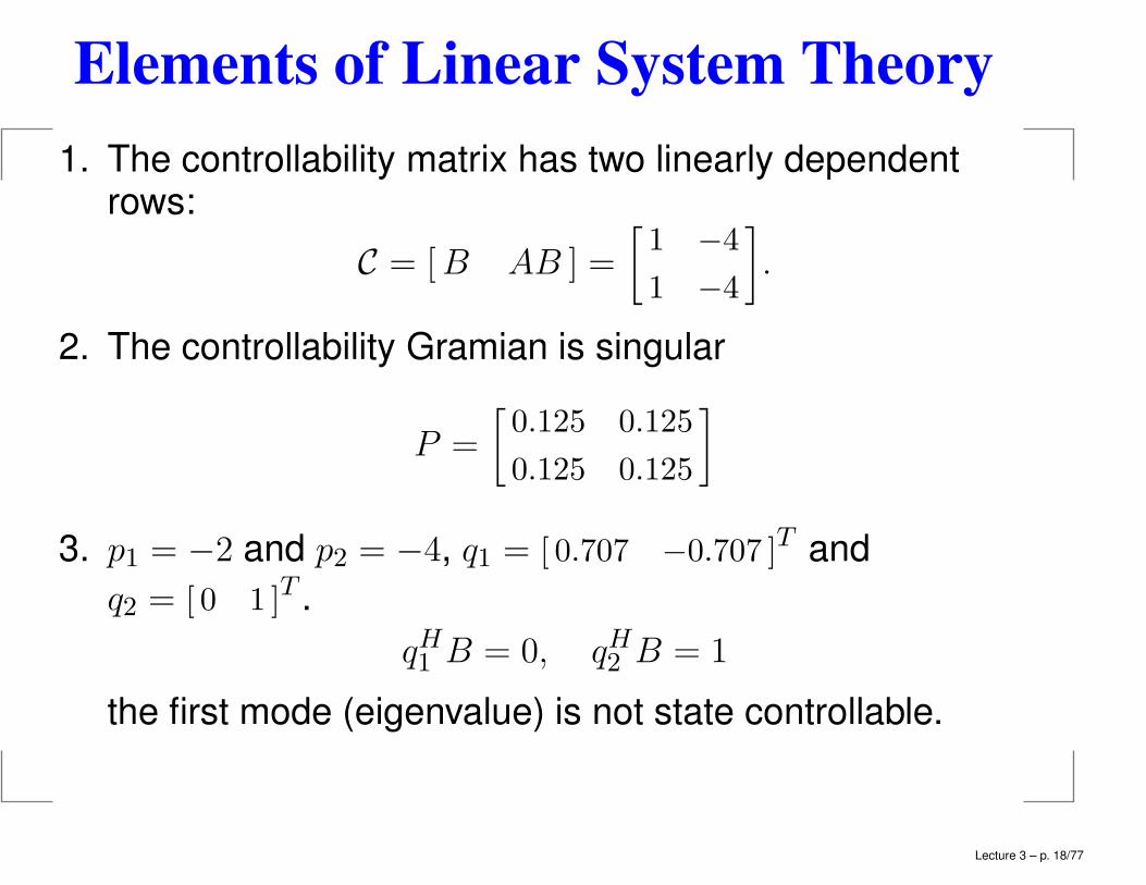
Elements of Linear System Theory
1. The controllability matrix has two linearly dependentrows:
C = [B AB ] =
[1 −4
1 −4
].
2. The controllability Gramian is singular
P =
[0.125 0.125
0.125 0.125
]
3. p1 = −2 and p2 = −4, q1 = [ 0.707 −0.707 ]T and
q2 = [ 0 1 ]T .
qH1 B = 0, qH2 B = 1
the first mode (eigenvalue) is not state controllable.
Lecture 3 – p. 18/77
Elements of Linear System Theory
Controllability is a system-theoretic concept important forcomputation and realizations; but no practical insight:
1. It says nothing about how the states behave, e.g. itdoes not imply that one can hold (as t → ∞) the statesat a given value.
2. Required inputs may be very large with suddenchanges.
3. Some states may be of no practical importance.
4. Existence result which provides no “degree ofcontrollability”.
Lecture 3 – p. 19/77
Elements of Linear System Theory
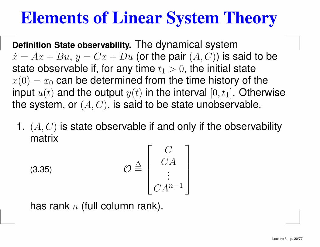
Definition State observability. The dynamical systemx = Ax+Bu, y = Cx+Du (or the pair (A,C)) is said to bestate observable if, for any time t1 > 0, the initial statex(0) = x0 can be determined from the time history of theinput u(t) and the output y(t) in the interval [0, t1]. Otherwisethe system, or (A,C), is said to be state unobservable.
1. (A,C) is state observable if and only if the observabilitymatrix
O∆=
CCA
...CAn−1
(3.35)
has rank n (full column rank).
Lecture 3 – p. 20/77
Elements of Linear System Theory
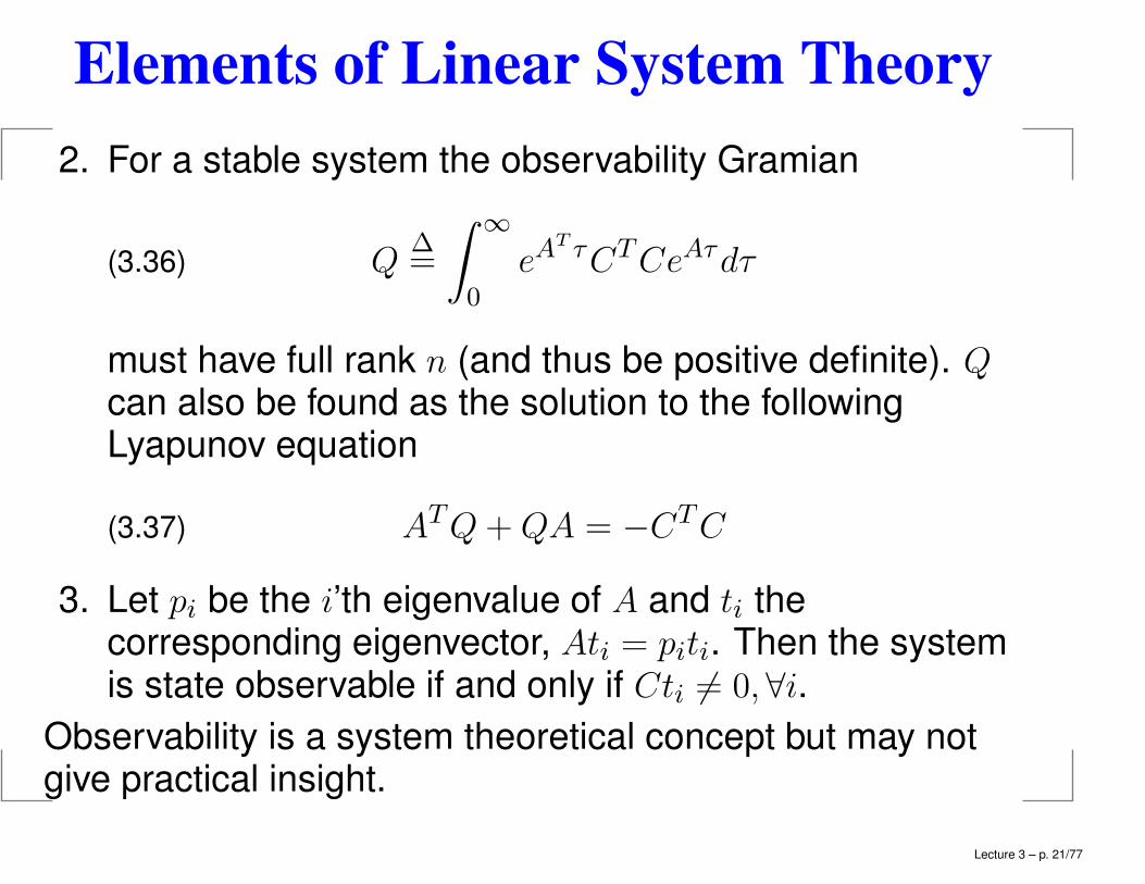
2. For a stable system the observability Gramian
Q∆=
∫ ∞
0
eAT τCTCeAτdτ(3.36)
must have full rank n (and thus be positive definite). Qcan also be found as the solution to the followingLyapunov equation
ATQ+QA = −CTC(3.37)
3. Let pi be the i’th eigenvalue of A and ti thecorresponding eigenvector, Ati = piti. Then the systemis state observable if and only if Cti 6= 0,∀i.
Observability is a system theoretical concept but may notgive practical insight.
Lecture 3 – p. 21/77
Elements of Linear System Theory
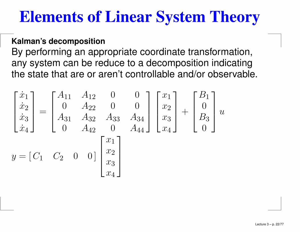
Kalman’s decomposition
By performing an appropriate coordinate transformation,any system can be reduce to a decomposition indicatingthe state that are or aren’t controllable and/or observable.
x1x2x3x4
=
A11 A12 0 00 A22 0 0
A31 A32 A33 A34
0 A42 0 A44
x1x2x3x4
+
B1
0B3
0
u
y = [C1 C2 0 0 ]
x1x2x3x4
Lecture 3 – p. 22/77
Elements of Linear System Theory
s1
s3
s2
s4
x1
x3
x2
x4
u y
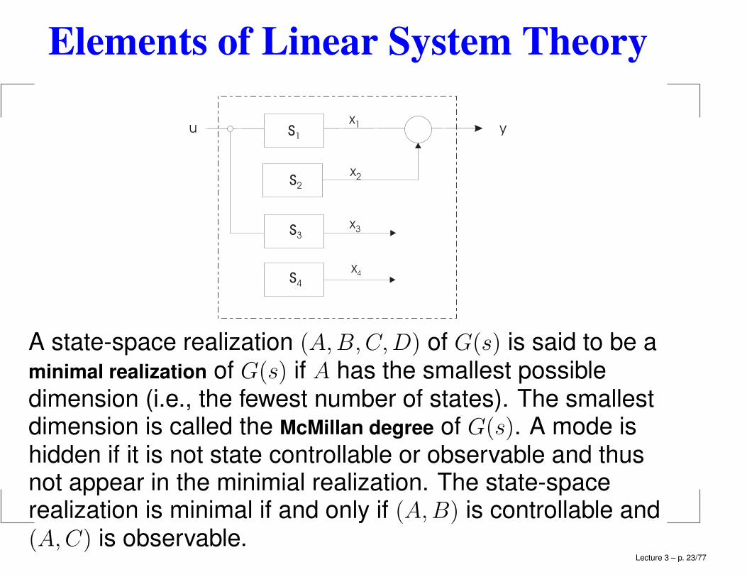
A state-space realization (A,B,C,D) of G(s) is said to be aminimal realization of G(s) if A has the smallest possibledimension (i.e., the fewest number of states). The smallestdimension is called the McMillan degree of G(s). A mode ishidden if it is not state controllable or observable and thusnot appear in the minimial realization. The state-spacerealization is minimal if and only if (A,B) is controllable and(A,C) is observable.
Lecture 3 – p. 23/77
Elements of Linear System Theory
3.3 Stability [4.3]
Definition
A system is (internally) stable if none of its componentscontains hidden unstable modes and the injection ofbounded external signals at any place in the system resultsin bounded output signals measured anywhere in thesystem. “internal”, i.e. all the states must be stable not onlyinputs/outputs.
Definition
State stabilizable, state detectable and hidden unstable modes. Asystem is state stabilizable if all unstable modes are statecontrollable. A system is state detectable if all unstablemodes are state observable. A system with unstabilizableor undetectable modes is said to contain hidden unstablemodes.
Lecture 3 – p. 24/77
Elements of Linear System Theory
3.4 Poles [4.4]
Definition
Poles. The poles pi of a system with state-space description(3.2)–(3.3) are the eigenvalues λi(A), i = 1, . . . , n of thematrix A. The pole or characteristic polynomial φ(s) is
defined as φ(s)∆= det(sI −A) =
∏ni=1(s− pi). Thus the poles
are the roots of the characteristic equation
φ(s)∆= det(sI − A) = 0(3.38)
Lecture 3 – p. 25/77
Elements of Linear System Theory
3.4.1 Poles and stability
Theorem 1 A linear dynamic system x = Ax+Bu is stableif and only if all the poles are in the open left-half plane(LHP), that is, Re{λi(A)} < 0,∀i. A matrix A with such aproperty is said to be “stable” or Hurwitz.
3.4.2 Poles from transfer functions
Theorem 2 The pole polynomial φ(s) corresponding to aminimal realization of a system with transfer function G(s),is the least common denominator of all non-identically-zerominors of all orders of G(s).
Lecture 3 – p. 26/77
Elements of Linear System Theory
Example:
G(s) =1
1.25(s+ 1)(s+ 2)
[s− 1 s−6 s− 2
](3.39)
The minors of order 1 are the four elements all have(s+ 1)(s+ 2) in the denominator.Minor of order 2
detG(s) =(s− 1)(s− 2) + 6s
1.252(s+ 1)2(s+ 2)2=
1
1.252(s+ 1)(s+ 2)(3.40)
Least common denominator of all the minors:
φ(s) = (s+ 1)(s+ 2)(3.41)
Minimal realization has two poles: s = −1; s = −2.
Lecture 3 – p. 27/77
Elements of Linear System Theory
Example: Consider the 2× 3 system, with 3 inputs and 2
outputs,
G(s) =1
(s+ 1)(s+ 2)(s− 1)∗
∗
[(s− 1)(s+ 2) 0 (s− 1)2
−(s+ 1)(s+ 2) (s− 1)(s+ 1) (s− 1)(s+ 1)
](3.42)
Minors of order 1:
1
s+ 1,
s− 1
(s+ 1)(s+ 2),
−1
s− 1,
1
s+ 2,
1
s+ 2(3.43)
Minor of order 2 corresponding to the deletion of column 2:
Lecture 3 – p. 28/77
Elements of Linear System Theory
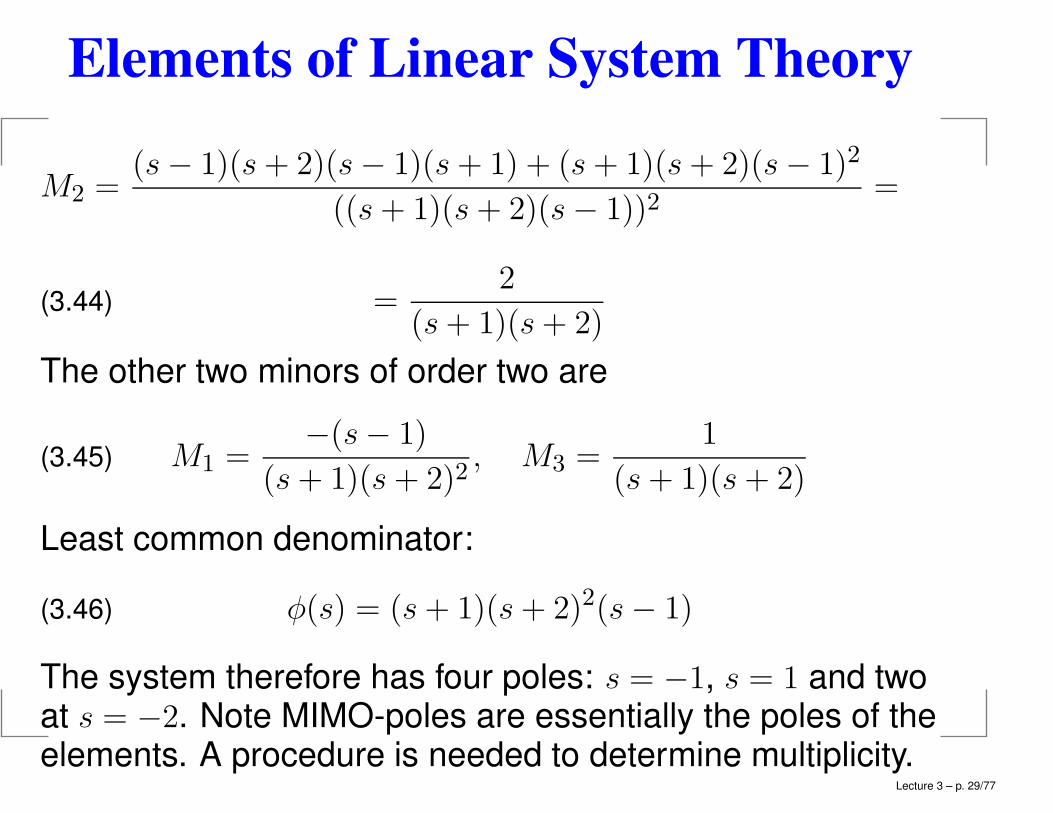
M2 =(s− 1)(s+ 2)(s− 1)(s+ 1) + (s+ 1)(s+ 2)(s− 1)2
((s+ 1)(s+ 2)(s− 1))2=
=2
(s+ 1)(s+ 2)(3.44)
The other two minors of order two are
M1 =−(s− 1)
(s+ 1)(s+ 2)2, M3 =
1
(s+ 1)(s+ 2)(3.45)
Least common denominator:
φ(s) = (s+ 1)(s+ 2)2(s− 1)(3.46)
The system therefore has four poles: s = −1, s = 1 and twoat s = −2. Note MIMO-poles are essentially the poles of theelements. A procedure is needed to determine multiplicity.
Lecture 3 – p. 29/77
Elements of Linear System Theory
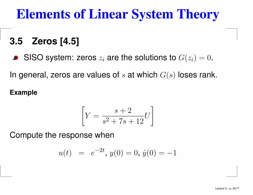
3.5 Zeros [4.5]
SISO system: zeros zi are the solutions to G(zi) = 0.
In general, zeros are values of s at which G(s) loses rank.
Example
[Y =
s+ 2
s2 + 7s+ 12U
]
Compute the response when
u(t) = e−2t, y(0) = 0, y(0) = −1
Lecture 3 – p. 30/77
Elements of Linear System Theory
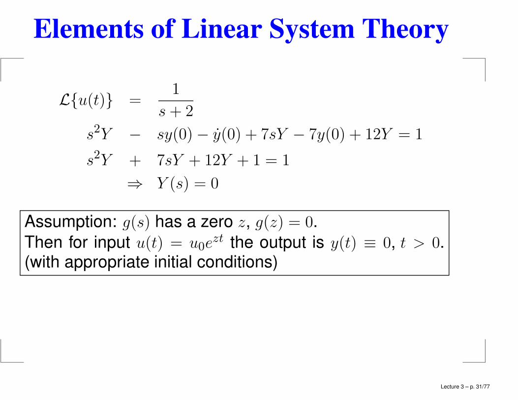
L{u(t)} =1
s+ 2
s2Y − sy(0)− y(0) + 7sY − 7y(0) + 12Y = 1
s2Y + 7sY + 12Y + 1 = 1
⇒ Y (s) = 0
Assumption: g(s) has a zero z, g(z) = 0.
Then for input u(t) = u0ezt the output is y(t) ≡ 0, t > 0.
(with appropriate initial conditions)
Lecture 3 – p. 31/77
Elements of Linear System Theory
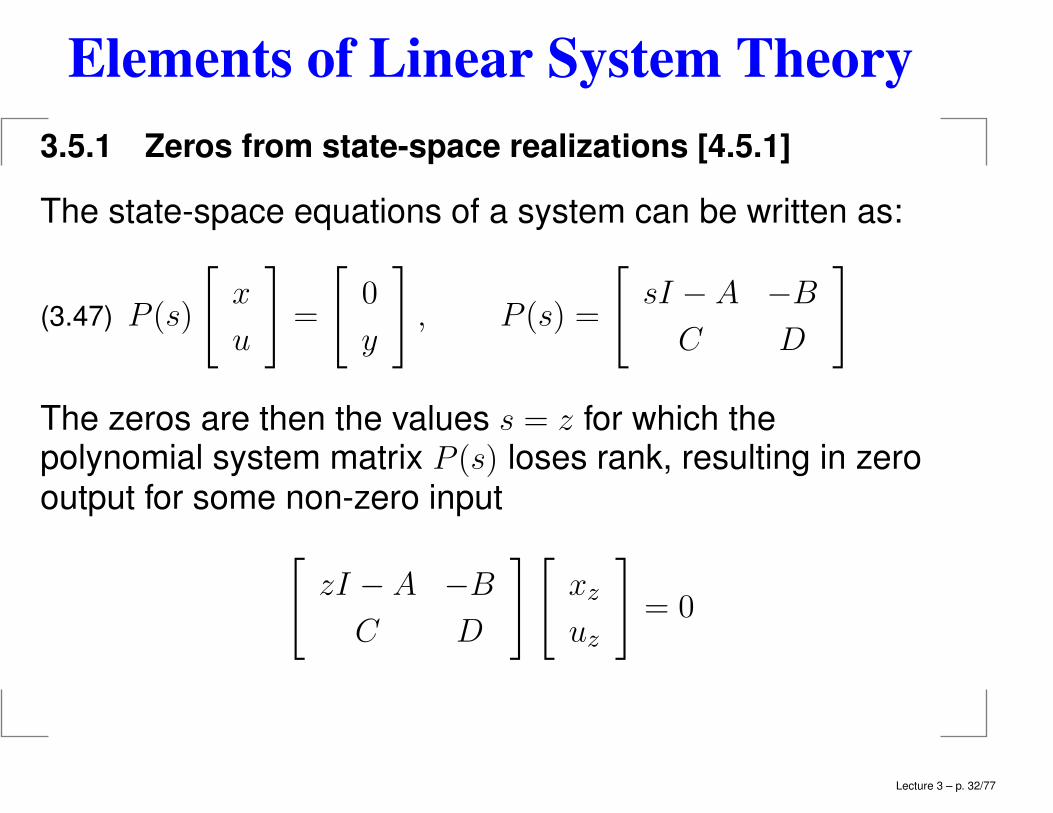
3.5.1 Zeros from state-space realizations [4.5.1]
The state-space equations of a system can be written as:
P (s)
[x
u
]=
[0
y
], P (s) =
[sI − A −B
C D
](3.47)
The zeros are then the values s = z for which thepolynomial system matrix P (s) loses rank, resulting in zerooutput for some non-zero input
[zI − A −B
C D
][xz
uz
]= 0
Lecture 3 – p. 32/77
Elements of Linear System Theory
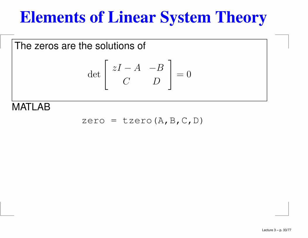
The zeros are the solutions of
det
[zI −A −B
C D
]= 0
MATLAB
zero = tzero(A,B,C,D)
Lecture 3 – p. 33/77
Elements of Linear System Theory
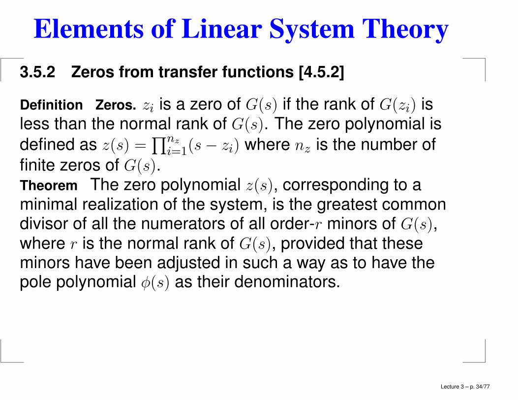
3.5.2 Zeros from transfer functions [4.5.2]
Definition Zeros. zi is a zero of G(s) if the rank of G(zi) isless than the normal rank of G(s). The zero polynomial is
defined as z(s) =∏nz
i=1(s− zi) where nz is the number of
finite zeros of G(s).Theorem The zero polynomial z(s), corresponding to aminimal realization of the system, is the greatest commondivisor of all the numerators of all order-r minors of G(s),where r is the normal rank of G(s), provided that theseminors have been adjusted in such a way as to have thepole polynomial φ(s) as their denominators.
Lecture 3 – p. 34/77
Elements of Linear System Theory
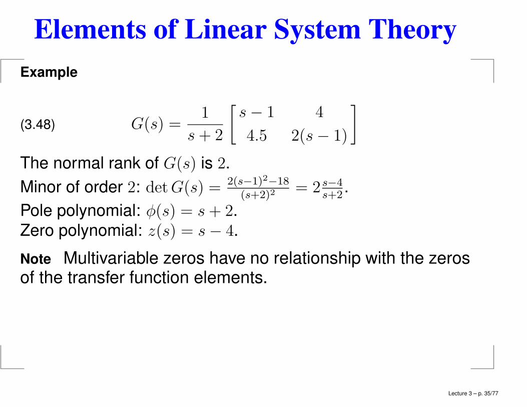
Example
G(s) =1
s+ 2
[s− 1 4
4.5 2(s− 1)
](3.48)
The normal rank of G(s) is 2.
Minor of order 2: detG(s) = 2(s−1)2−18(s+2)2
= 2 s−4s+2
.
Pole polynomial: φ(s) = s+ 2.
Zero polynomial: z(s) = s− 4.
Note Multivariable zeros have no relationship with the zerosof the transfer function elements.
Lecture 3 – p. 35/77
Elements of Linear System Theory
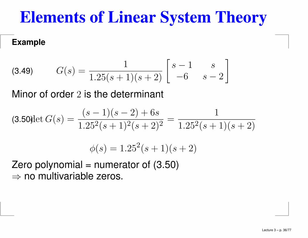
Example
G(s) =1
1.25(s+ 1)(s+ 2)
[s− 1 s−6 s− 2
](3.49)
Minor of order 2 is the determinant
detG(s) =(s− 1)(s− 2) + 6s
1.252(s+ 1)2(s+ 2)2=
1
1.252(s+ 1)(s+ 2)(3.50)
φ(s) = 1.252(s+ 1)(s+ 2)
Zero polynomial = numerator of (3.50)⇒ no multivariable zeros.
Lecture 3 – p. 36/77
Elements of Linear System Theory
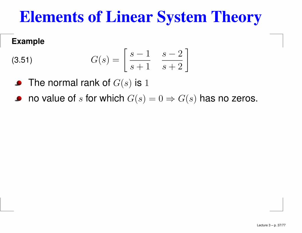
Example
G(s) =
[s− 1
s+ 1
s− 2
s+ 2
](3.51)
The normal rank of G(s) is 1
no value of s for which G(s) = 0 ⇒ G(s) has no zeros.
Lecture 3 – p. 37/77
Elements of Linear System Theory
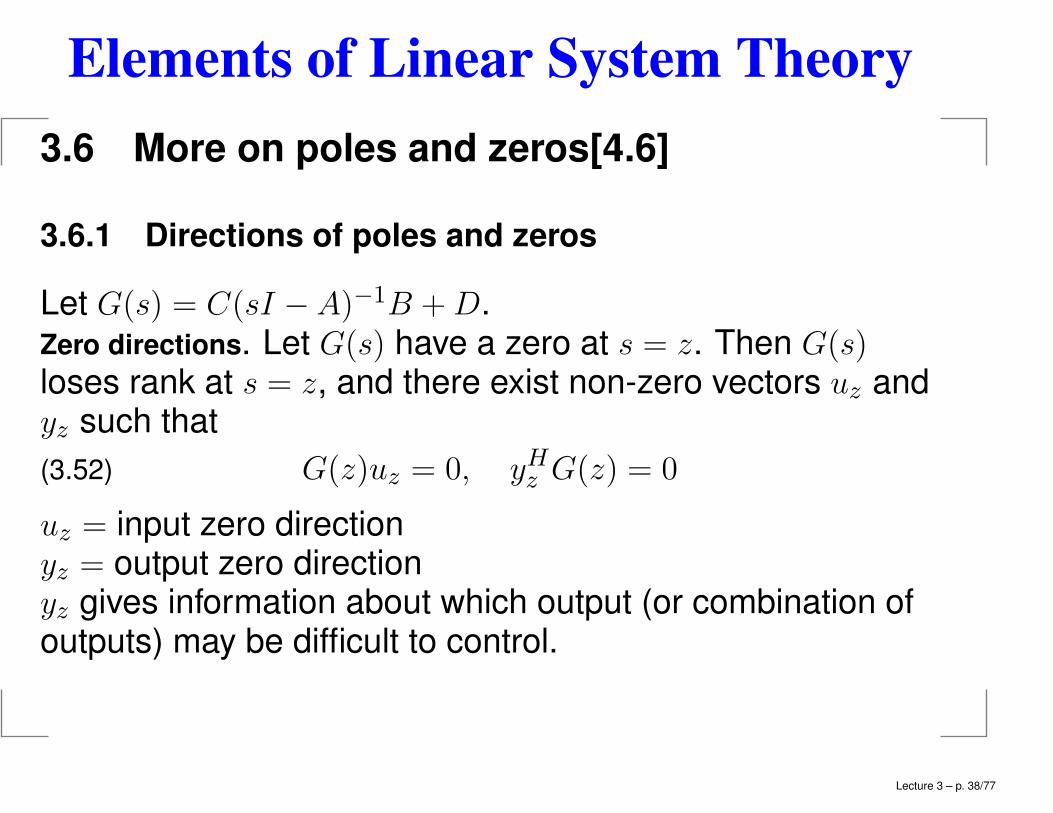
3.6 More on poles and zeros[4.6]
3.6.1 Directions of poles and zeros
Let G(s) = C(sI −A)−1B +D.Zero directions. Let G(s) have a zero at s = z. Then G(s)loses rank at s = z, and there exist non-zero vectors uz andyz such that
G(z)uz = 0, yHz G(z) = 0(3.52)
uz = input zero directionyz = output zero directionyz gives information about which output (or combination ofoutputs) may be difficult to control.
Lecture 3 – p. 38/77
Elements of Linear System Theory
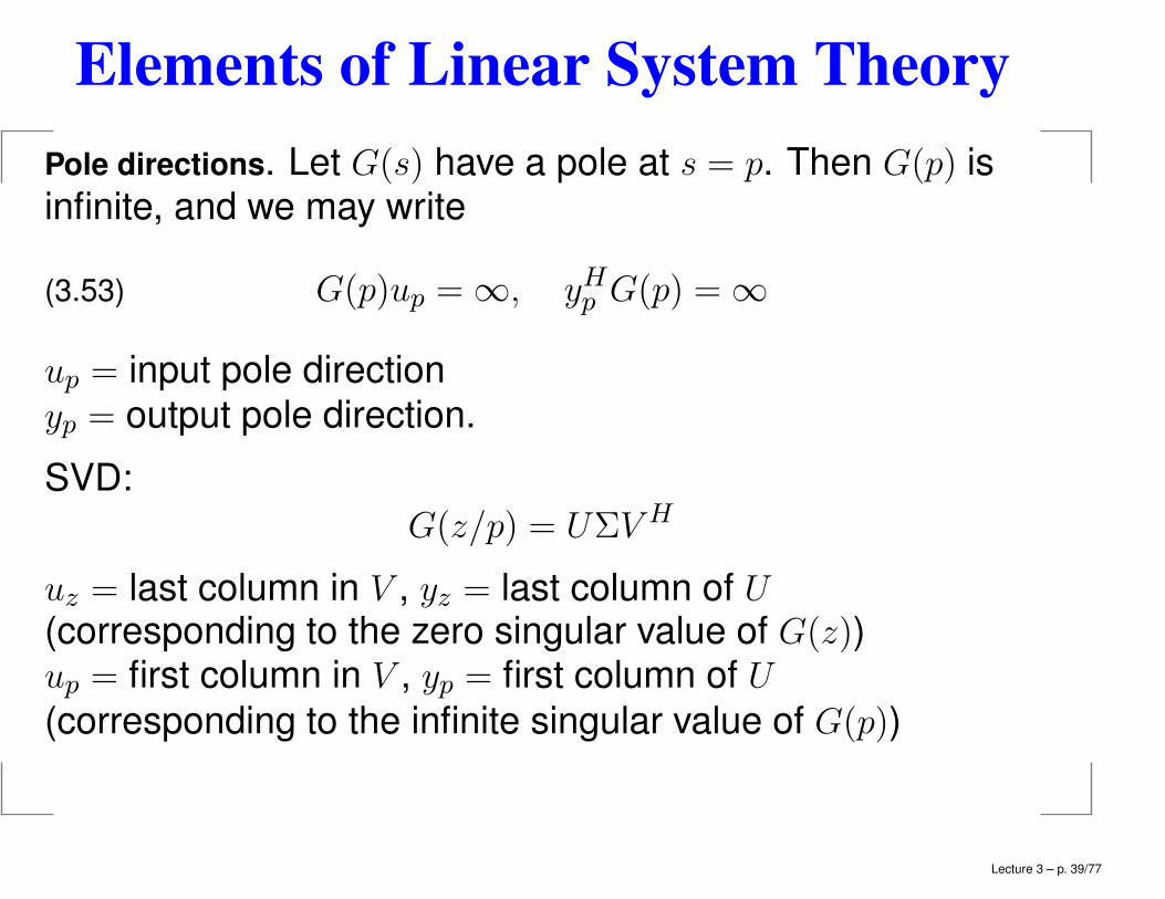
Pole directions. Let G(s) have a pole at s = p. Then G(p) isinfinite, and we may write
G(p)up = ∞, yHp G(p) = ∞(3.53)
up = input pole directionyp = output pole direction.
SVD:
G(z/p) = UΣV H
uz = last column in V , yz = last column of U(corresponding to the zero singular value of G(z))up = first column in V , yp = first column of U
(corresponding to the infinite singular value of G(p))
Lecture 3 – p. 39/77
Elements of Linear System Theory
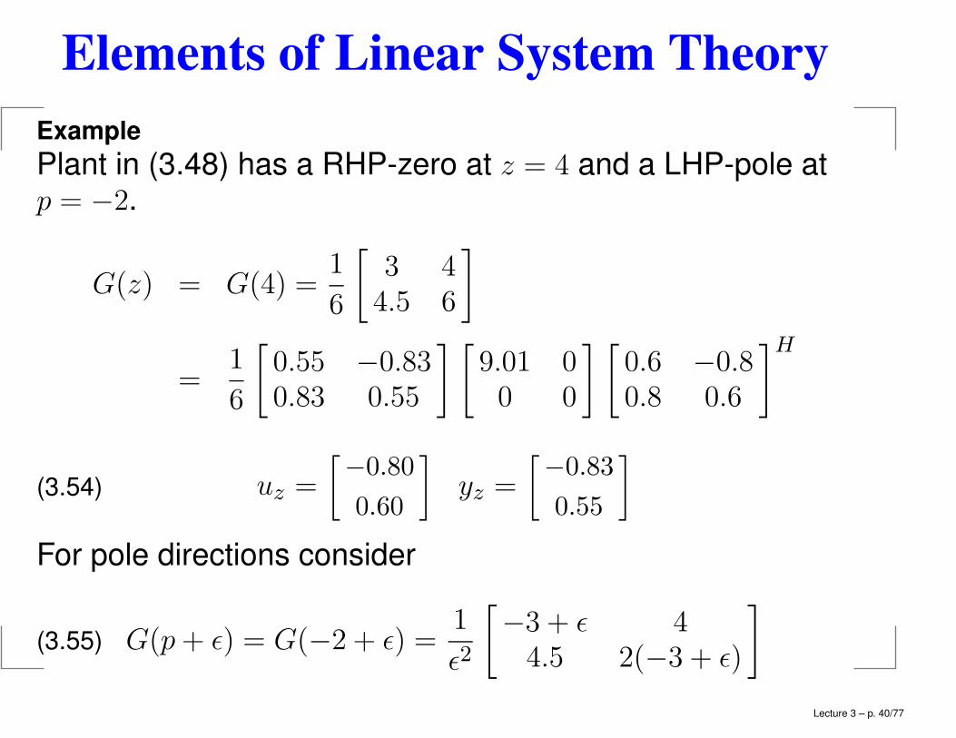
Example
Plant in (3.48) has a RHP-zero at z = 4 and a LHP-pole atp = −2.
G(z) = G(4) =1
6
[3 44.5 6
]
=1
6
[0.55 −0.830.83 0.55
] [9.01 00 0
] [0.6 −0.80.8 0.6
]H
uz =
[−0.80
0.60
]yz =
[−0.83
0.55
](3.54)
For pole directions consider
G(p+ ǫ) = G(−2 + ǫ) =1
ǫ2
[−3 + ǫ 44.5 2(−3 + ǫ)
](3.55)
Lecture 3 – p. 40/77
Elements of Linear System Theory
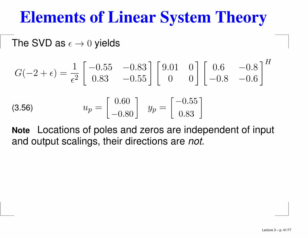
The SVD as ǫ → 0 yields
G(−2 + ǫ) =1
ǫ2
[−0.55 −0.830.83 −0.55
] [9.01 00 0
] [0.6 −0.8−0.8 −0.6
]H
up =
[0.60
−0.80
]yp =
[−0.55
0.83
](3.56)
Note Locations of poles and zeros are independent of inputand output scalings, their directions are not.
Lecture 3 – p. 41/77
Elements of Linear System Theory
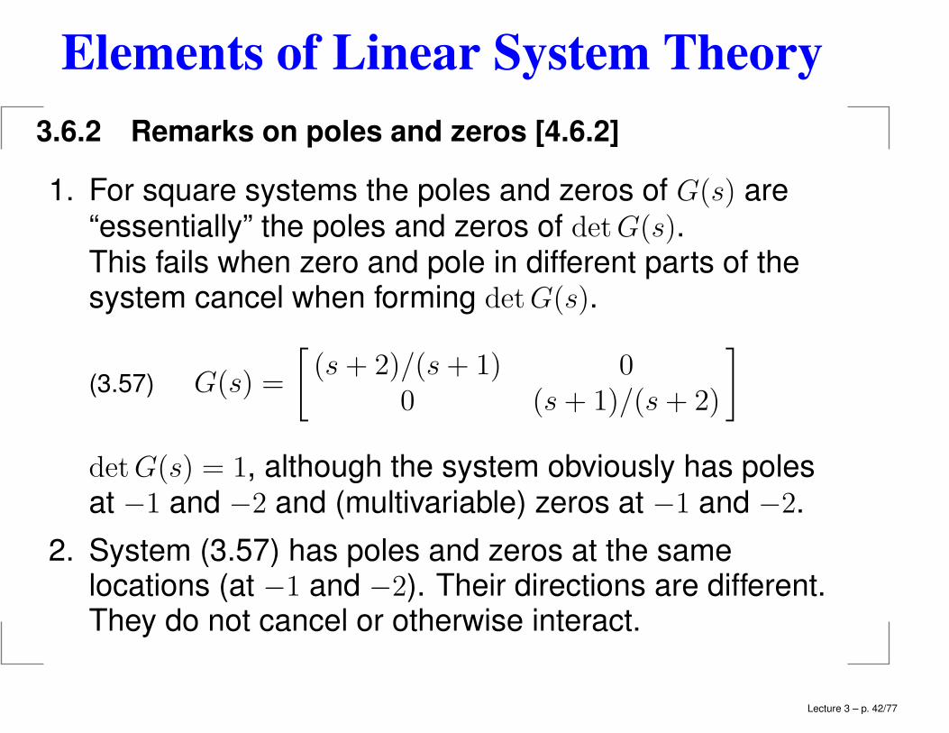
3.6.2 Remarks on poles and zeros [4.6.2]
1. For square systems the poles and zeros of G(s) are“essentially” the poles and zeros of detG(s).This fails when zero and pole in different parts of thesystem cancel when forming detG(s).
G(s) =
[(s+ 2)/(s+ 1) 0
0 (s+ 1)/(s+ 2)
](3.57)
detG(s) = 1, although the system obviously has polesat −1 and −2 and (multivariable) zeros at −1 and −2.
2. System (3.57) has poles and zeros at the samelocations (at −1 and −2). Their directions are different.They do not cancel or otherwise interact.
Lecture 3 – p. 42/77
Elements of Linear System Theory
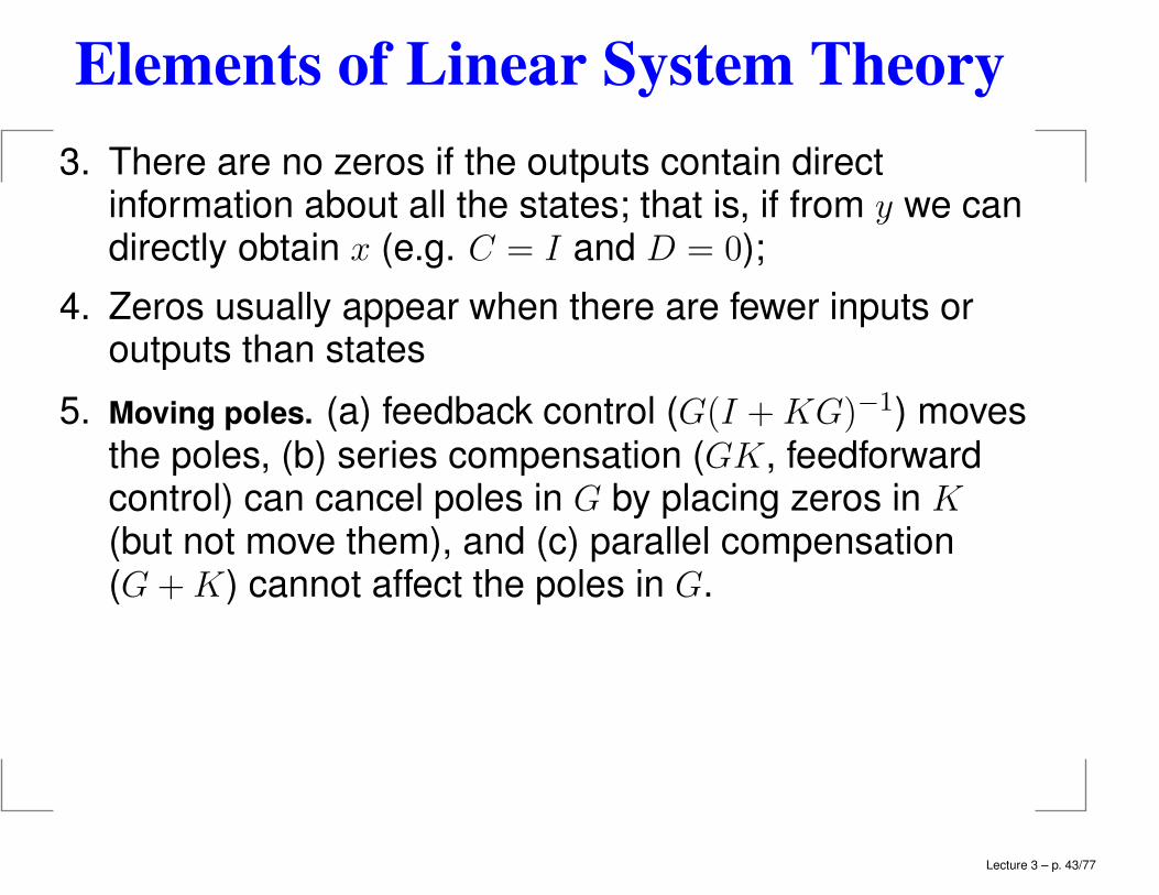
3. There are no zeros if the outputs contain directinformation about all the states; that is, if from y we candirectly obtain x (e.g. C = I and D = 0);
4. Zeros usually appear when there are fewer inputs oroutputs than states
5. Moving poles. (a) feedback control (G(I +KG)−1) movesthe poles, (b) series compensation (GK, feedforwardcontrol) can cancel poles in G by placing zeros in K(but not move them), and (c) parallel compensation(G+K) cannot affect the poles in G.
Lecture 3 – p. 43/77
Elements of Linear System Theory
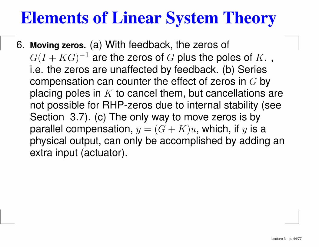
6. Moving zeros. (a) With feedback, the zeros of
G(I +KG)−1 are the zeros of G plus the poles of K. ,i.e. the zeros are unaffected by feedback. (b) Seriescompensation can counter the effect of zeros in G byplacing poles in K to cancel them, but cancellations arenot possible for RHP-zeros due to internal stability (seeSection 3.7). (c) The only way to move zeros is byparallel compensation, y = (G+K)u, which, if y is aphysical output, can only be accomplished by adding anextra input (actuator).
Lecture 3 – p. 44/77
Elements of Linear System Theory
Example. Effect of feedback on poles and zeros.
SISO plant G(s) = z(s)/φ(s) and K(s) = k.
T (s) =L(s)
1 + L(s)=
kG(s)
1 + kG(s)=
kz(s)
φ(s) + kz(s)= k
zcl(s)
φcl(s)(3.58)
Note the following:1. Zero polynomial: zcl(s) = z(s)
⇒ zero locations are unchanged.
2. Pole locations are changed by feedback.For example,
k → 0 ⇒ φcl(s) → φ(s)(3.59)
k → ∞ ⇒ φcl(s) → z(s).z(s)(3.60)
where roots of z(s) move with k to infinity (complex pattern)(cf. root locus)
Lecture 3 – p. 45/77
Elements of Linear System Theory
3.7 Internal stability of feedback systems [4.7]
Note: Checking the pole of S or T is not sufficient todetermine internal stability
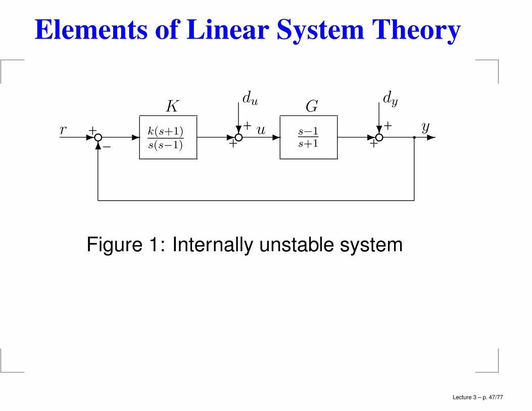
Example (Figure 1). In forming L = GK we cancel the term
(s− 1) (a RHP pole-zero cancellation) to obtain
L = GK =k
s, and S = (I + L)−1 =
s
s+ k(3.61)
S(s) is stable, i.e. transfer function from dy to y is stable.
However, the transfer function from dy to u is unstable:
u = −K(I +GK)−1dy = −k(s+ 1)
(s− 1)(s+ k)dy(3.62)
Lecture 3 – p. 46/77
Elements of Linear System Theory
❞❞❞ q
✻✲❄❄ ✲✲✲✲✲ +
+
+
++-
yu
dydu G
s−1s+1
k(s+1)s(s−1)
K
r
Figure 1: Internally unstable system
Lecture 3 – p. 47/77
Elements of Linear System Theory
❞
❞q
q
✻✛ ✛
❄
❄✲✲✻
+
+
+
+
y
dy u
du
G
−K
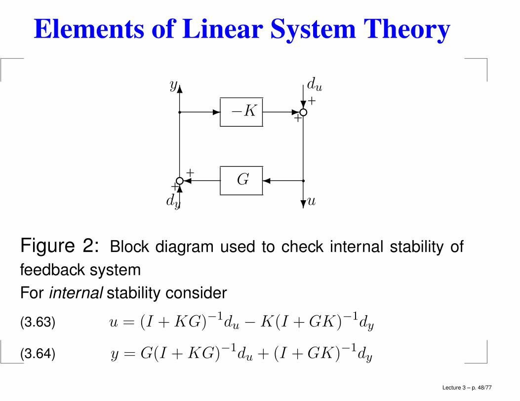
Figure 2: Block diagram used to check internal stability of
feedback system
For internal stability consider
u = (I +KG)−1du −K(I +GK)−1dy(3.63)
y = G(I +KG)−1du + (I +GK)−1dy(3.64)
Lecture 3 – p. 48/77
Elements of Linear System Theory
Theorem 4.4 The feedback system in Figure 2 is internally
stable if and only if all four closed-loop transfer matrices in(3.63) and (3.64) are stable.
Theorem 4.5 Assume there are no RHP pole-zerocancellations between G(s) and K(s). Then the feedbacksystem in Figure 2 is internally stable if and only if one of thefour closed-loop transfer function matrices in (3.63) and (3.64)is stable.
Lecture 3 – p. 49/77
Elements of Linear System Theory
Implications of the internal stability requirement
1. If G(s) has a RHP-zero at z, then L = GK,
T = GK(I +GK)−1, SG = (I +GK)−1G, LI = KG and
TI = KG(I +KG)−1 will each have a RHP-zero at z.
2. If G(s) has a RHP-pole at p, then L = GK and LI = KGalso have a RHP-pole at p, while
S = (I +GK)−1,KS = K(I +GK)−1 and
SI = (I +KG)−1 have a RHP-zero at p.
Lecture 3 – p. 50/77
Elements of Linear System Theory
Exercise: Interpolation constraints. Prove for SISO feedback
systems when the plant G(s) has a RHP-zero z or a
RHP-pole p:
G(z) = 0 ⇒ L(z) = 0 ⇔ T (z) = 0, S(z) = 1(3.65)
G−1(p) = 0 ⇒ L(p) = ∞ ⇔ T (p) = 1, S(p) = 0(3.66)
Remark “Perfect control” implies S ≈ 0 and T ≈ 1.RHP-zero ⇒ perfect control impossible.RHP-pole ⇒ perfect control possible.RHP-poles cause problems when tight (high gain) control isnot possible.
Lecture 3 – p. 51/77
Elements of Linear System Theory
3.8 Stabilizing controllers [4.8]
Stable plantsLemma For a stable plant G(s) the negative feedback systemin Figure 2 is internally stable if and only if
Q = K(I +GK)−1 is stable.Proof: The four transfer functions in (3.63) and (3.64) are
K(I +GK)−1 = Q(3.67)
(I +GK)−1 = I −GQ(3.68)
(I +KG)−1 = I −QG(3.69)
G(I +KG)−1 = G(I −QG)(3.70)
which are clearly all stable if and only if G and Q are stable.
Lecture 3 – p. 52/77
Elements of Linear System Theory
Consequences: All stabilizing negative feedback controllersfor the stable plant G(s) are given by
K = (I −QG)−1Q = Q(I −GQ)−1(3.71)
where the “parameter” Q is any stable transfer function matrix.(Identical to the internal model control (IMC)parameterization of stabilizing controllers.)
Lecture 3 – p. 53/77
Elements of Linear System Theory
❞
❞
❞ q q❄ ✲✲✻
❄✲✲
✲✲✲+
+
dy
-
+
model
G-
+
yplant
GQ
K
r
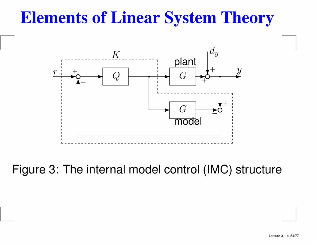
Figure 3: The internal model control (IMC) structure
Lecture 3 – p. 54/77
Elements of Linear System Theory
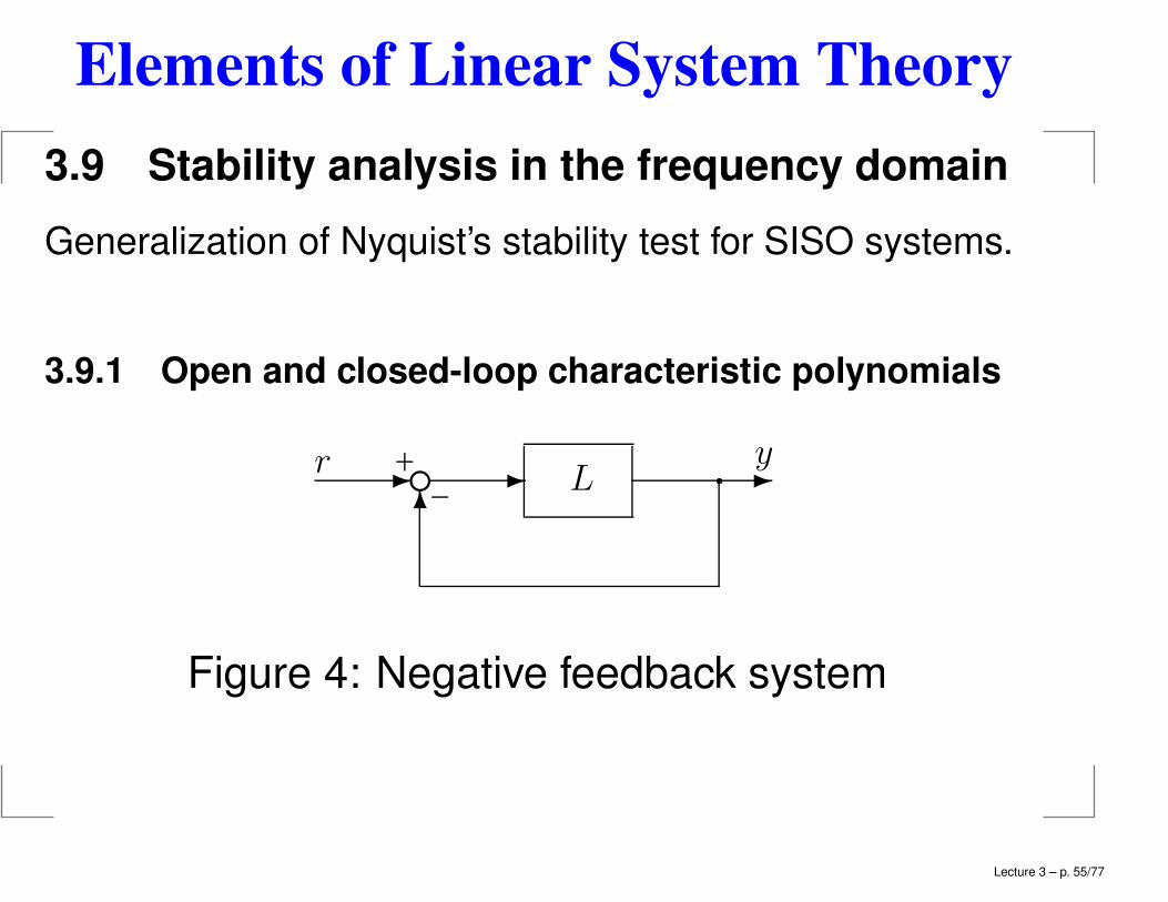
3.9 Stability analysis in the frequency domain
Generalization of Nyquist’s stability test for SISO systems.
3.9.1 Open and closed-loop characteristic polynomials
❡ q
✻✲✲✲ y
L-
+r
Figure 4: Negative feedback system
Lecture 3 – p. 55/77
Elements of Linear System Theory
Open Loop:
L(s) = Col(sI −Aol)−1Bol +Dol(3.72)
Poles of L(s) are the roots of the open-loop characteristicpolynomial
φol(s) = det(sI − Aol)(3.73)
Assume no RHP pole-zero cancellations between G(s) andK(s). Then from Theorem 4.5 internal stability of theclosed-loop system is equivalent to the stability of
S(s) = (I + L(s))−1.The realization of S(s) can be derived as follow:
x = Aolx+Bol(r − y)(3.74)
−e = r − y = r − Colx−Dol(r − y)(3.75)
Lecture 3 – p. 56/77
Elements of Linear System Theory
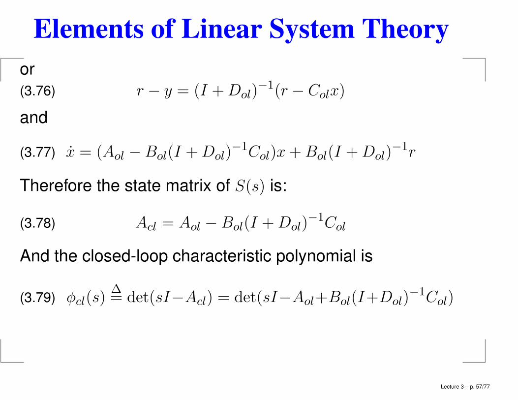
or
r − y = (I +Dol)−1(r − Colx)(3.76)
and
x = (Aol −Bol(I +Dol)−1Col)x+Bol(I +Dol)
−1r(3.77)
Therefore the state matrix of S(s) is:
Acl = Aol − Bol(I +Dol)−1Col(3.78)
And the closed-loop characteristic polynomial is
φcl(s)∆= det(sI−Acl) = det(sI−Aol+Bol(I+Dol)
−1Col)(3.79)
Lecture 3 – p. 57/77
Elements of Linear System Theory
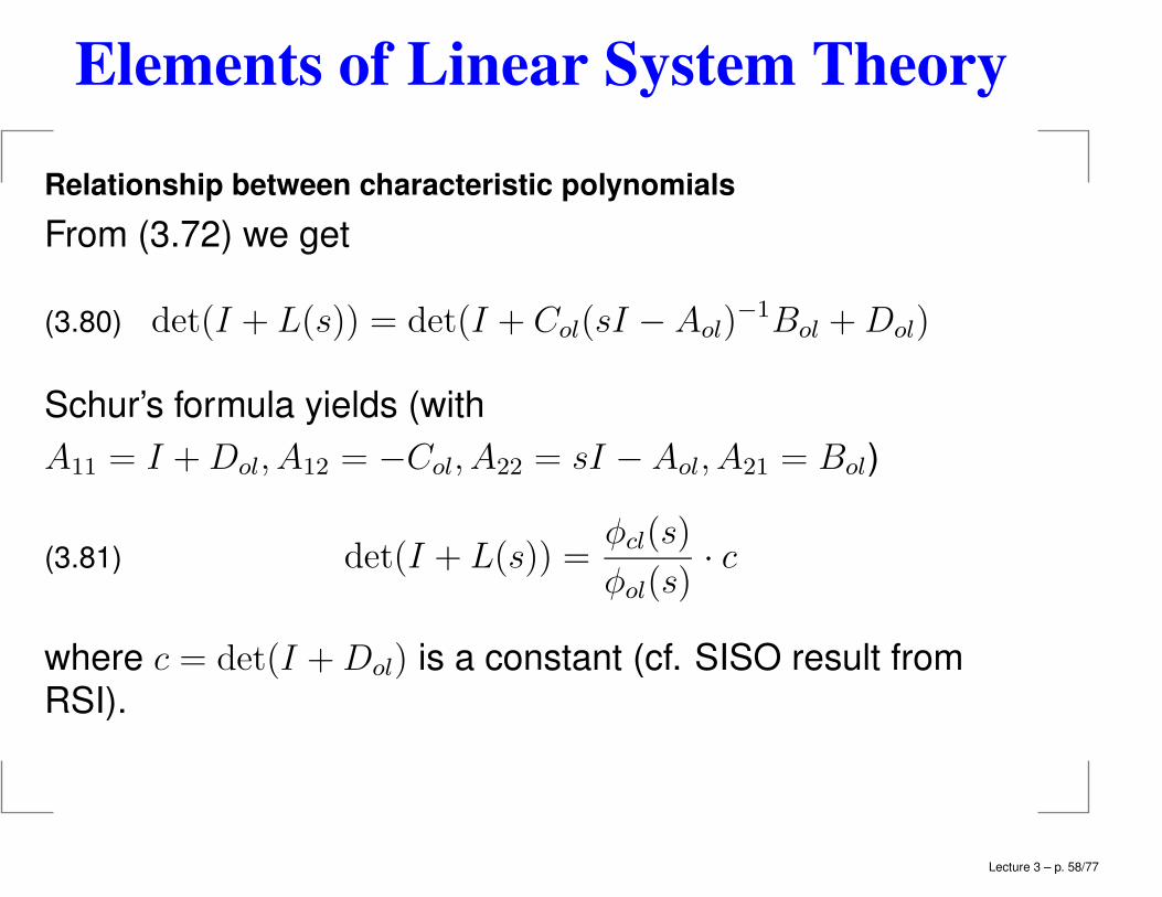
Relationship between characteristic polynomials
From (3.72) we get
det(I + L(s)) = det(I + Col(sI − Aol)−1Bol +Dol)(3.80)
Schur’s formula yields (with
A11 = I +Dol, A12 = −Col, A22 = sI −Aol, A21 = Bol)
det(I + L(s)) =φcl(s)
φol(s)· c(3.81)
where c = det(I +Dol) is a constant (cf. SISO result fromRSI).
Lecture 3 – p. 58/77
Elements of Linear System Theory
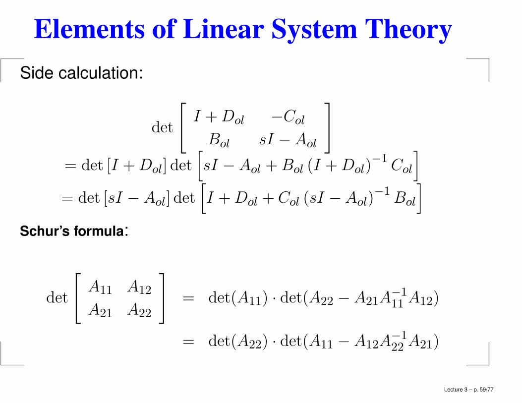
Side calculation:
det
[I +Dol −Col
Bol sI − Aol
]
= det [I +Dol] det[sI −Aol +Bol (I +Dol)
−1Col
]
= det [sI − Aol] det[I +Dol + Col (sI − Aol)
−1Bol
]
Schur’s formula:
det
[A11 A12
A21 A22
]= det(A11) · det(A22 − A21A
−111 A12)
= det(A22) · det(A11 − A12A−122 A21)
Lecture 3 – p. 59/77
Elements of Linear System Theory
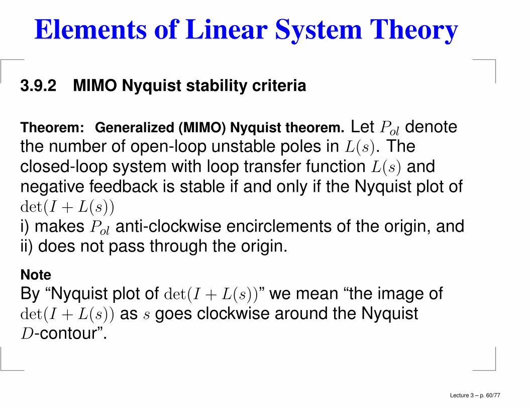
3.9.2 MIMO Nyquist stability criteria
Theorem: Generalized (MIMO) Nyquist theorem. Let Pol denotethe number of open-loop unstable poles in L(s). Theclosed-loop system with loop transfer function L(s) andnegative feedback is stable if and only if the Nyquist plot ofdet(I + L(s))i) makes Pol anti-clockwise encirclements of the origin, andii) does not pass through the origin.
Note
By “Nyquist plot of det(I + L(s))” we mean “the image ofdet(I + L(s)) as s goes clockwise around the NyquistD-contour”.
Lecture 3 – p. 60/77
Elements of Linear System Theory
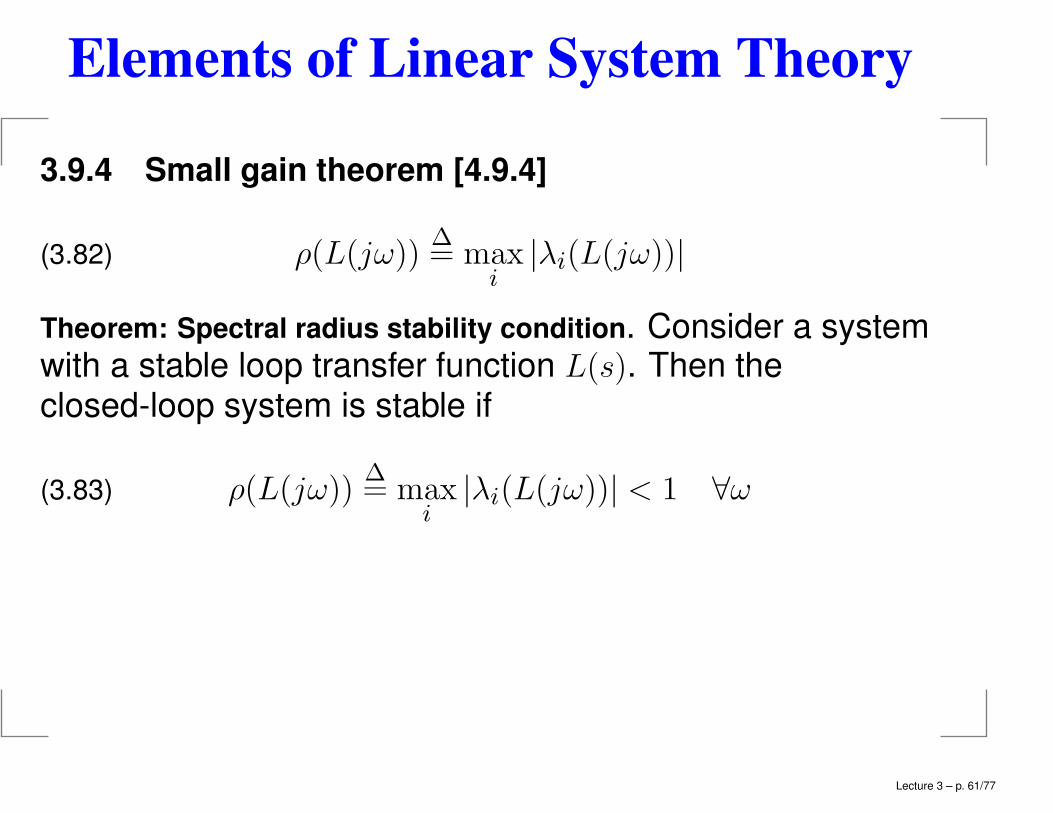
3.9.4 Small gain theorem [4.9.4]
ρ(L(jω))∆= max
i|λi(L(jω))|(3.82)
Theorem: Spectral radius stability condition. Consider a systemwith a stable loop transfer function L(s). Then theclosed-loop system is stable if
ρ(L(jω))∆= max
i|λi(L(jω))| < 1 ∀ω(3.83)
Lecture 3 – p. 61/77
Elements of Linear System Theory
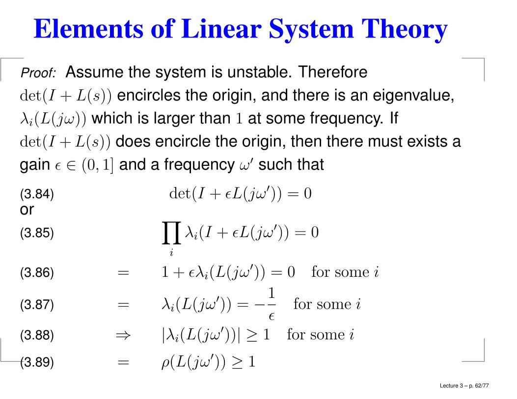
Proof: Assume the system is unstable. Therefore
det(I + L(s)) encircles the origin, and there is an eigenvalue,
λi(L(jω)) which is larger than 1 at some frequency. If
det(I +L(s)) does encircle the origin, then there must exists a
gain ǫ ∈ (0, 1] and a frequency ω′ such that
det(I + ǫL(jω′)) = 0(3.84)
or ∏
i
λi(I + ǫL(jω′)) = 0(3.85)
= 1 + ǫλi(L(jω′)) = 0 for some i(3.86)
= λi(L(jω′)) = −
1
ǫfor some i(3.87)
⇒ |λi(L(jω′))| ≥ 1 for some i(3.88)
= ρ(L(jω′)) ≥ 1(3.89)
Lecture 3 – p. 62/77
Elements of Linear System Theory
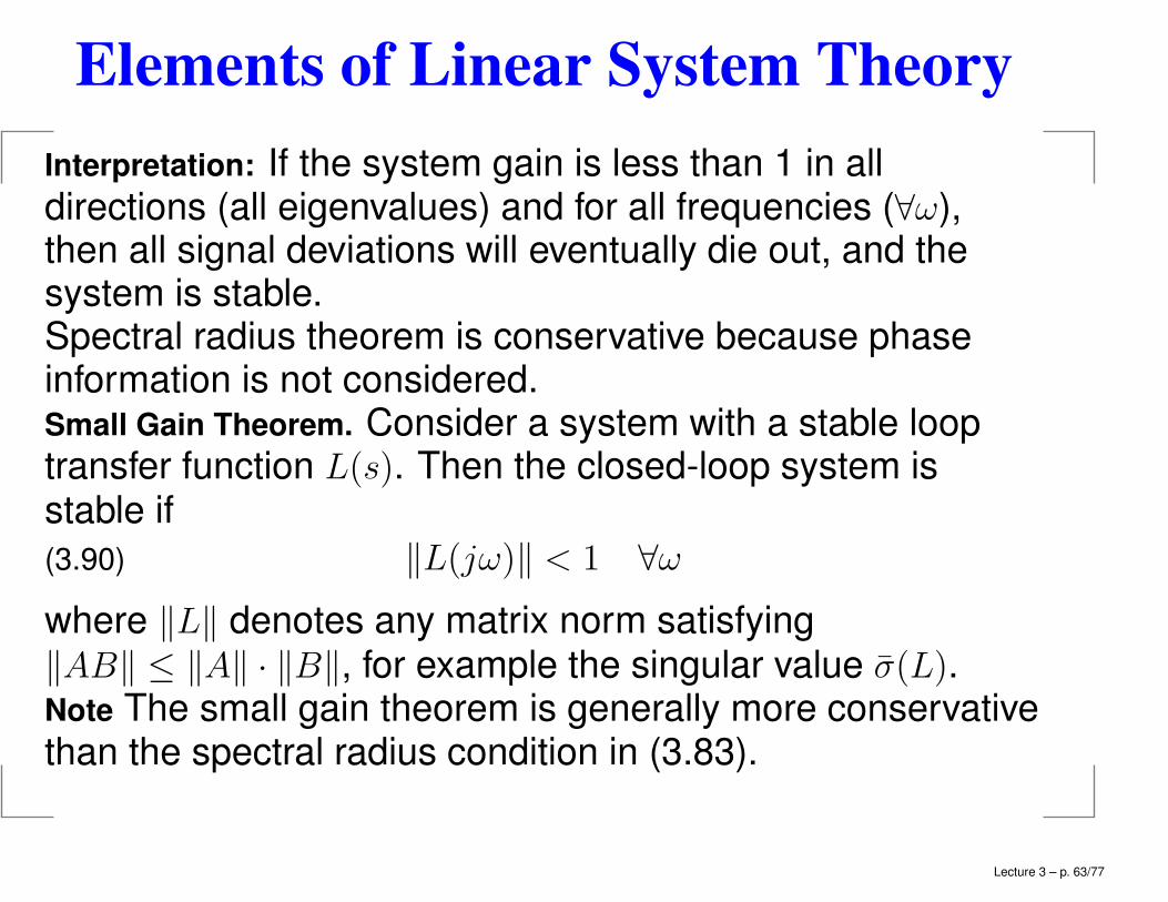
Interpretation: If the system gain is less than 1 in alldirections (all eigenvalues) and for all frequencies (∀ω),then all signal deviations will eventually die out, and thesystem is stable.Spectral radius theorem is conservative because phaseinformation is not considered.Small Gain Theorem. Consider a system with a stable looptransfer function L(s). Then the closed-loop system isstable if
‖L(jω)‖ < 1 ∀ω(3.90)
where ‖L‖ denotes any matrix norm satisfying‖AB‖ ≤ ‖A‖ · ‖B‖, for example the singular value σ(L).Note The small gain theorem is generally more conservativethan the spectral radius condition in (3.83).
Lecture 3 – p. 63/77
Elements of Linear System Theory
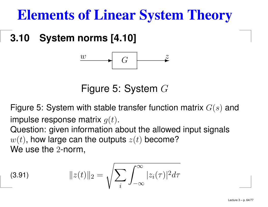
3.10 System norms [4.10]
✲✲ zw G
Figure 5: System G
Figure 5: System with stable transfer function matrix G(s) and
impulse response matrix g(t).Question: given information about the allowed input signalsw(t), how large can the outputs z(t) become?We use the 2-norm,
‖z(t)‖2 =
√∑
i
∫ ∞
−∞
|zi(τ)|2dτ(3.91)
Lecture 3 – p. 64/77
Elements of Linear System Theory
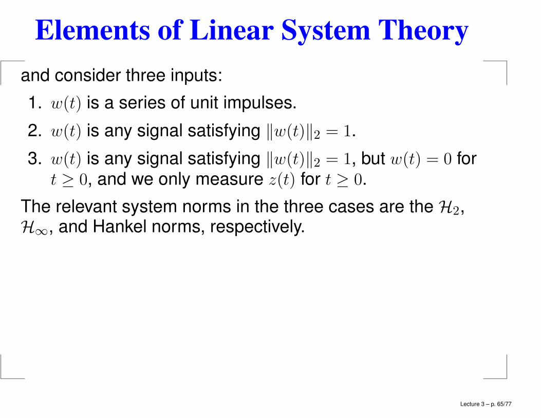
and consider three inputs:
1. w(t) is a series of unit impulses.
2. w(t) is any signal satisfying ‖w(t)‖2 = 1.
3. w(t) is any signal satisfying ‖w(t)‖2 = 1, but w(t) = 0 fort ≥ 0, and we only measure z(t) for t ≥ 0.
The relevant system norms in the three cases are the H2,H∞, and Hankel norms, respectively.
Lecture 3 – p. 65/77
Elements of Linear System Theory
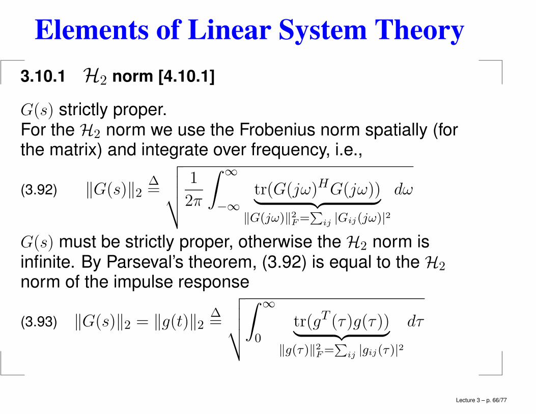
3.10.1 H2 norm [4.10.1]
G(s) strictly proper.For the H2 norm we use the Frobenius norm spatially (forthe matrix) and integrate over frequency, i.e.,
‖G(s)‖2∆=
√√√√1
2π
∫ ∞
−∞
tr(G(jω)HG(jω))︸ ︷︷ ︸‖G(jω)‖2F=
∑ij |Gij(jω)|2
dω(3.92)
G(s) must be strictly proper, otherwise the H2 norm isinfinite. By Parseval’s theorem, (3.92) is equal to the H2
norm of the impulse response
‖G(s)‖2 = ‖g(t)‖2∆=
√√√√∫ ∞
0
tr(gT (τ)g(τ))︸ ︷︷ ︸‖g(τ)‖2F=
∑ij |gij(τ)|
2
dτ(3.93)
Lecture 3 – p. 66/77
Elements of Linear System Theory
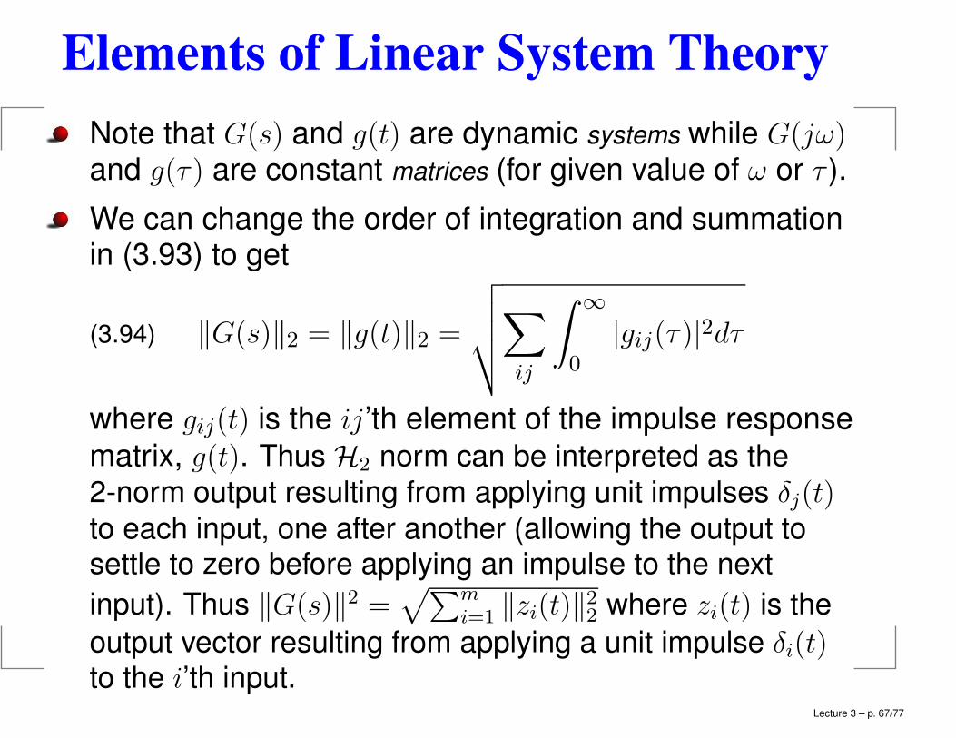
Note that G(s) and g(t) are dynamic systems while G(jω)and g(τ) are constant matrices (for given value of ω or τ ).
We can change the order of integration and summationin (3.93) to get
‖G(s)‖2 = ‖g(t)‖2 =
√√√√∑
ij
∫ ∞
0
|gij(τ)|2dτ(3.94)
where gij(t) is the ij’th element of the impulse response
matrix, g(t). Thus H2 norm can be interpreted as the
2-norm output resulting from applying unit impulses δj(t)to each input, one after another (allowing the output tosettle to zero before applying an impulse to the next
input). Thus ‖G(s)‖2 =√∑m
i=1 ‖zi(t)‖22 where zi(t) is the
output vector resulting from applying a unit impulse δi(t)to the i’th input.
Lecture 3 – p. 67/77
Elements of Linear System Theory
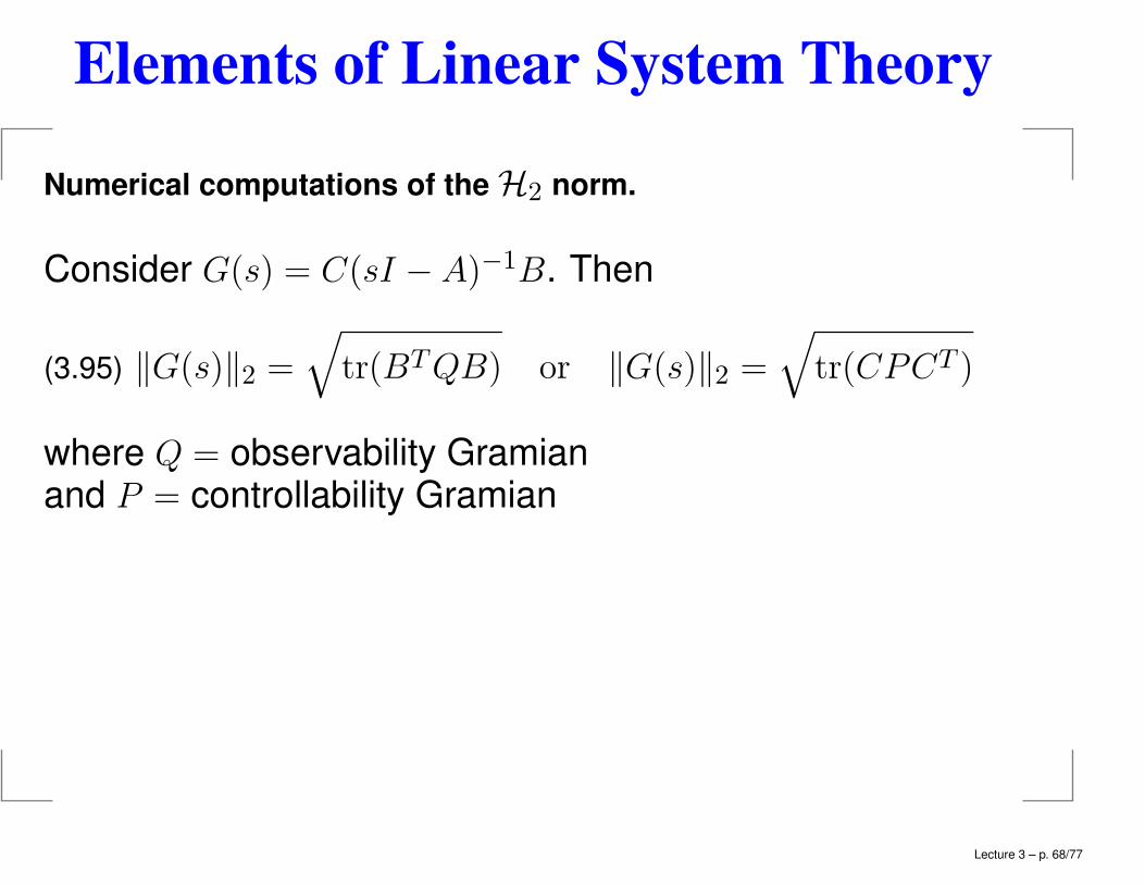
Numerical computations of the H2 norm.
Consider G(s) = C(sI − A)−1B. Then
‖G(s)‖2 =
√tr(BTQB) or ‖G(s)‖2 =
√tr(CPCT )(3.95)
where Q = observability Gramianand P = controllability Gramian
Lecture 3 – p. 68/77
Elements of Linear System Theory
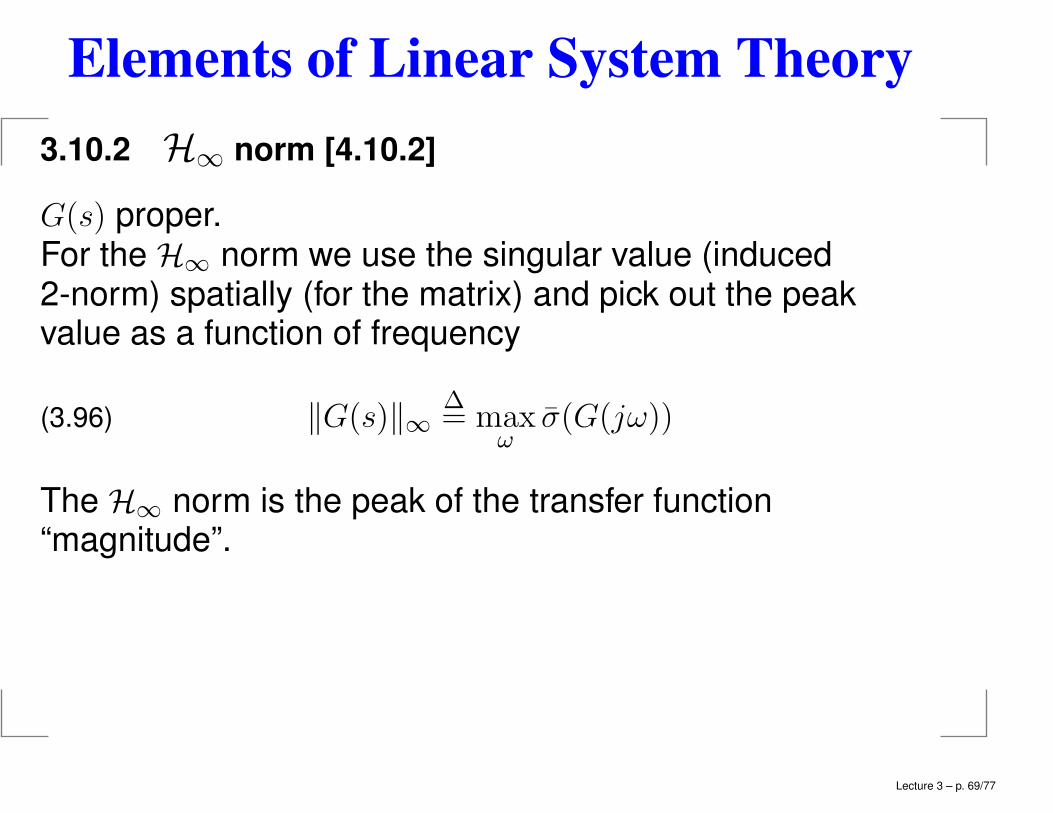
3.10.2 H∞ norm [4.10.2]
G(s) proper.For the H∞ norm we use the singular value (induced2-norm) spatially (for the matrix) and pick out the peakvalue as a function of frequency
‖G(s)‖∞∆= max
ωσ(G(jω))(3.96)
The H∞ norm is the peak of the transfer function“magnitude”.
Lecture 3 – p. 69/77
Elements of Linear System Theory
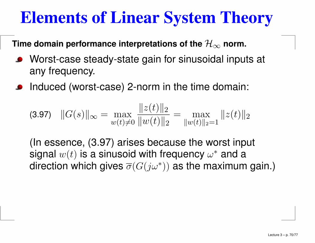
Time domain performance interpretations of the H∞ norm.
Worst-case steady-state gain for sinusoidal inputs atany frequency.
Induced (worst-case) 2-norm in the time domain:
‖G(s)‖∞ = maxw(t) 6=0
‖z(t)‖2‖w(t)‖2
= max‖w(t)‖2=1
‖z(t)‖2(3.97)
(In essence, (3.97) arises because the worst inputsignal w(t) is a sinusoid with frequency ω∗ and adirection which gives σ(G(jω∗)) as the maximum gain.)
Lecture 3 – p. 70/77
Elements of Linear System Theory
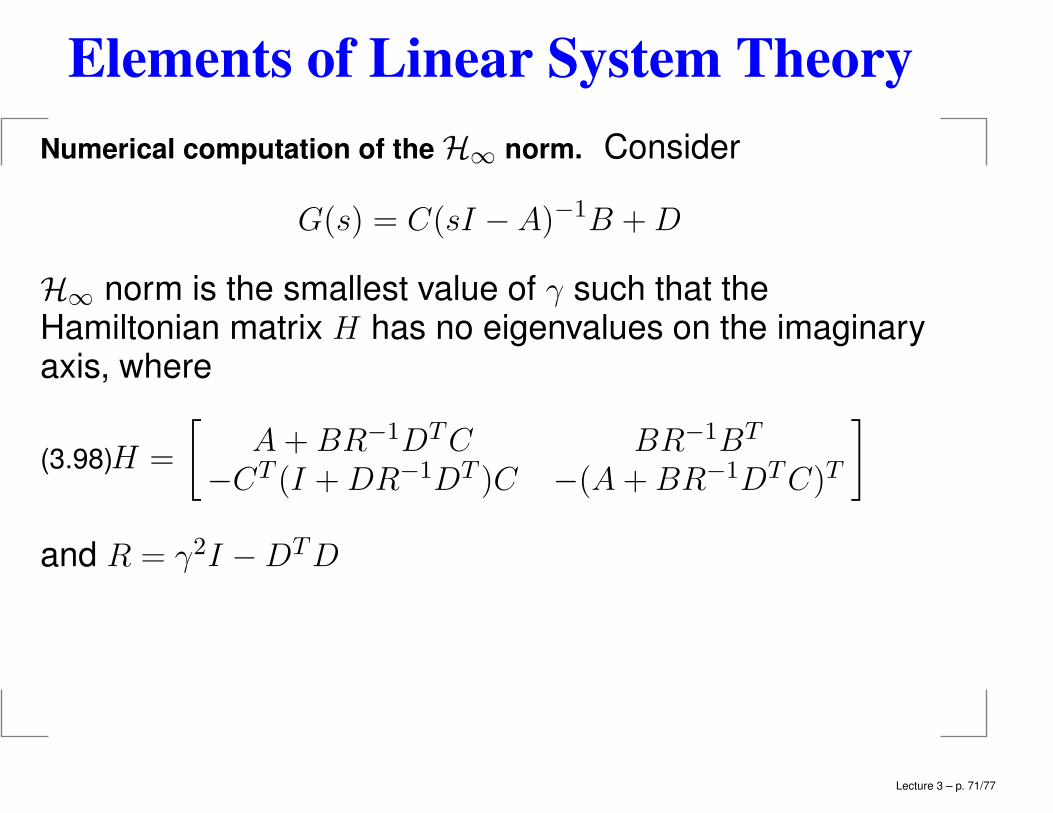
Numerical computation of the H∞ norm. Consider
G(s) = C(sI −A)−1B +D
H∞ norm is the smallest value of γ such that theHamiltonian matrix H has no eigenvalues on the imaginaryaxis, where
H =
[A+ BR−1DTC BR−1BT
−CT (I +DR−1DT )C −(A+BR−1DTC)T
](3.98)
and R = γ2I −DTD
Lecture 3 – p. 71/77
Elements of Linear System Theory
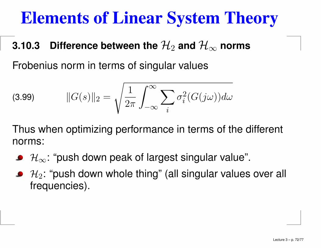
3.10.3 Difference between the H2 and H∞ norms
Frobenius norm in terms of singular values
‖G(s)‖2 =
√1
2π
∫ ∞
−∞
∑
i
σ2i (G(jω))dω(3.99)
Thus when optimizing performance in terms of the differentnorms:
H∞: “push down peak of largest singular value”.
H2: “push down whole thing” (all singular values over allfrequencies).
Lecture 3 – p. 72/77
Elements of Linear System Theory
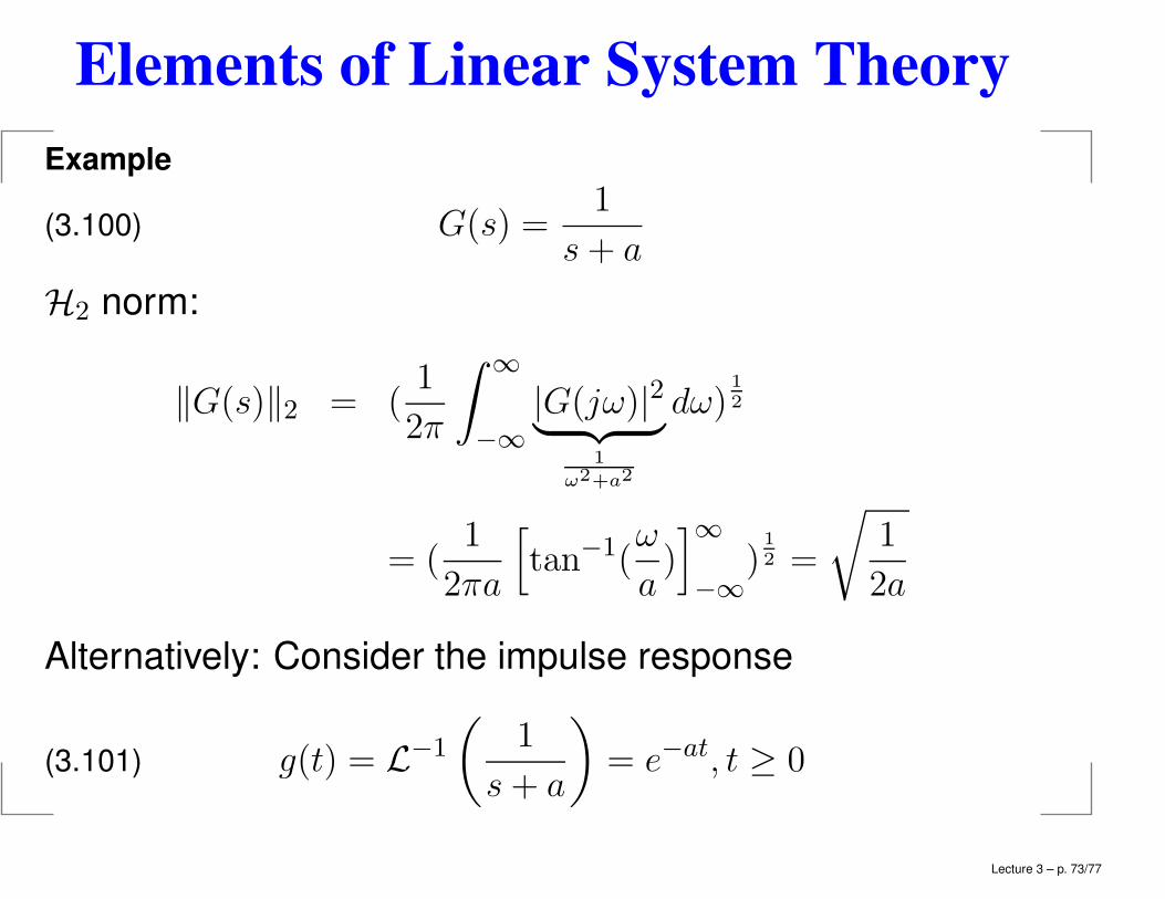
Example
G(s) =1
s+ a(3.100)
H2 norm:
‖G(s)‖2 = (1
2π
∫ ∞
−∞
|G(jω)|2︸ ︷︷ ︸1
ω2+a2
dω)1
2
= (1
2πa
[tan−1(
ω
a)]∞−∞
)1
2 =
√1
2a
Alternatively: Consider the impulse response
g(t) = L−1
(1
s+ a
)= e−at, t ≥ 0(3.101)
Lecture 3 – p. 73/77
Elements of Linear System Theory
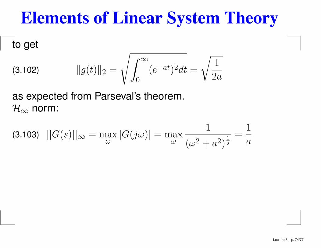
to get
‖g(t)‖2 =
√∫ ∞
0
(e−at)2dt =
√1
2a(3.102)
as expected from Parseval’s theorem.H∞ norm:
||G(s)||∞ = maxω
|G(jω)| = maxω
1
(ω2 + a2)1
2
=1
a(3.103)
Lecture 3 – p. 74/77
Elements of Linear System Theory
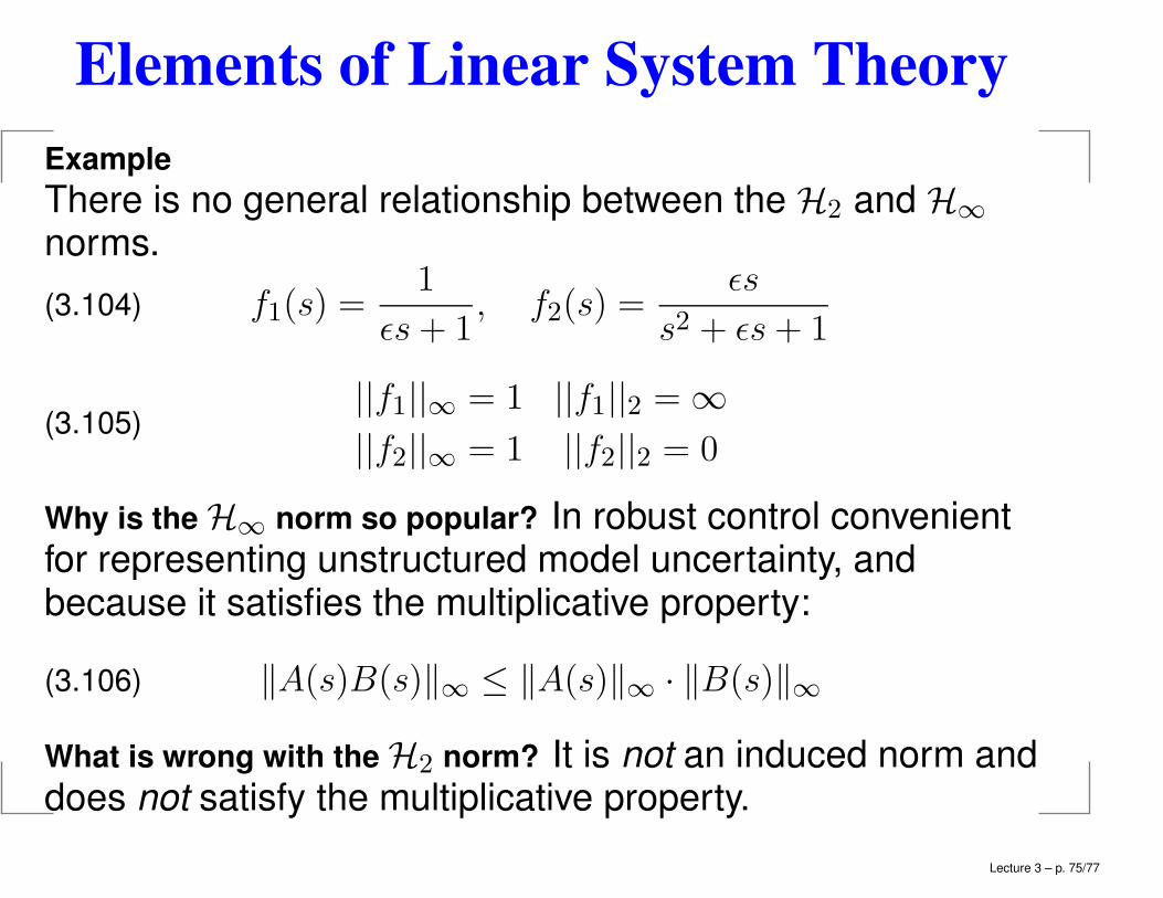
Example
There is no general relationship between the H2 and H∞
norms.
f1(s) =1
ǫs+ 1, f2(s) =
ǫs
s2 + ǫs+ 1(3.104)
||f1||∞ = 1 ||f1||2 = ∞
||f2||∞ = 1 ||f2||2 = 0(3.105)
Why is the H∞ norm so popular? In robust control convenientfor representing unstructured model uncertainty, andbecause it satisfies the multiplicative property:
‖A(s)B(s)‖∞ ≤ ‖A(s)‖∞ · ‖B(s)‖∞(3.106)
What is wrong with the H2 norm? It is not an induced norm anddoes not satisfy the multiplicative property.
Lecture 3 – p. 75/77
Elements of Linear System Theory
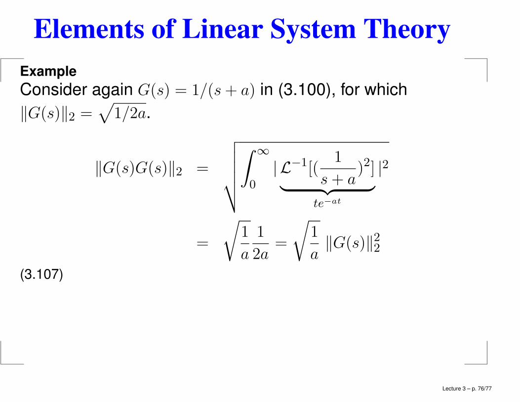
Example
Consider again G(s) = 1/(s+ a) in (3.100), for which
‖G(s)‖2 =√
1/2a.
‖G(s)G(s)‖2 =
√√√√√
∫ ∞
0
| L−1[(1
s+ a)2]
︸ ︷︷ ︸te−at
|2
=
√1
a
1
2a=
√1
a‖G(s)‖22
(3.107)
Lecture 3 – p. 76/77
Elements of Linear System Theory
for a < 1,
‖G(s)G(s)‖2 > ‖G(s)‖2 · ‖G(s)‖2(3.108)
which does not satisfy the multiplicative property.H∞ norm does satisfy the multiplicative property
‖G(s)G(s)‖∞ =1
a2= ‖G(s)‖∞ · ‖G(s)‖∞
Lecture 3 – p. 77/77