![Σύντομο Εγχειρίδιο SPSS 16 - old.psych.uoa.grold.psych.uoa.gr/~roussosp//stats/Manual_SPSS16.pdf · Σύντομο Εγχειρίδιο spss 16.0 [3] Δυο λόγια](https://static.fdocument.org/doc/165x107/5b5a6aa97f8b9a2d458b8b63/-spss-16-oldpsychuoagroldpsychuoagrroussospstatsmanual.jpg)
SPSS Workshop Research Support Center Chongming Yang.
34
SPSS Workshop Research Support Center Chongming Yang
-
Upload
amir-rumley -
Category
Documents
-
view
233 -
download
0
Transcript of SPSS Workshop Research Support Center Chongming Yang.
SPSS Workshop
Research Support CenterChongming Yang
Causal Inference
• If A, then B, under condition C
• If A, 95% Probability B, under condition C
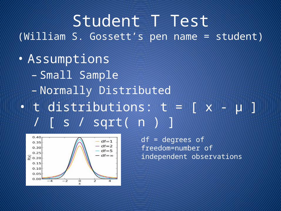
Student T Test(William S. Gossett’s pen name = student)
• Assumptions– Small Sample – Normally Distributed
• t distributions: t = [ x - μ ] / [ s / sqrt( n ) ]
df = degrees of freedom=number of independent observations
Type of T Tests
• One sample – test against a specific (population) mean
• Two independent samples – compare means of two independent samples that
represent two populations
• Paired – compare means of repeated samples
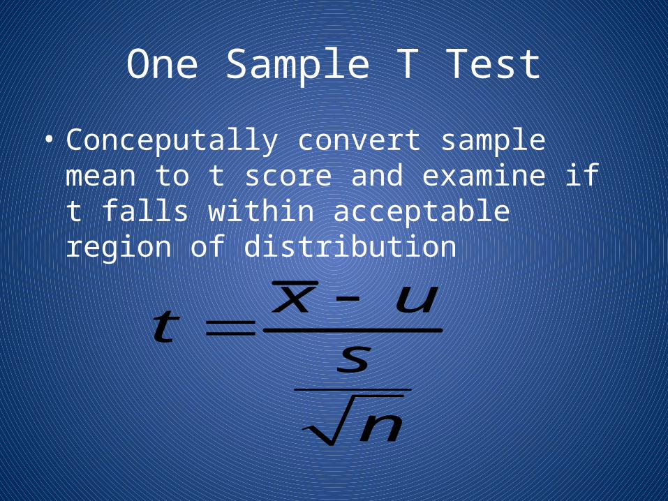
One Sample T Test
• Conceputally convert sample mean to t score and examine if t falls within acceptable region of distribution
x ut
s
n
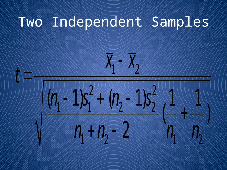
Two Independent Samples
1 2
2 21 1 2 2
1 2 1 2
( 1) ( 1) 1 1( )
2
x xt
n s n sn n n n
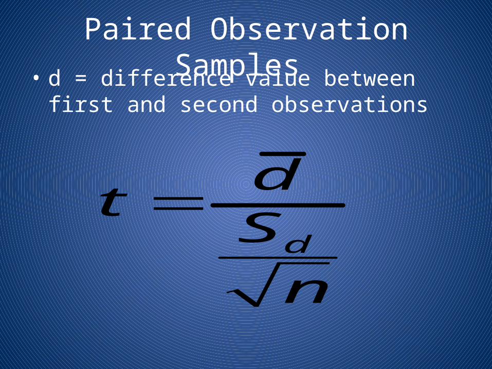
Paired Observation Samples • d = difference value between first and second
observations
d
dt
S
n
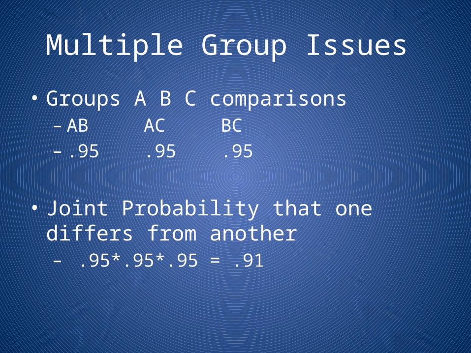
Multiple Group Issues
• Groups A B C comparisons – AB AC BC – .95 .95 .95
• Joint Probability that one differs from another – .95*.95*.95 = .91
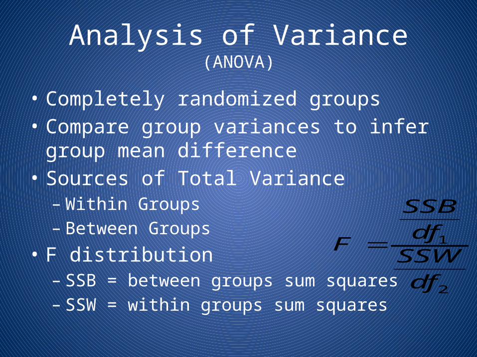
Analysis of Variance(ANOVA)
• Completely randomized groups • Compare group variances to infer group mean
difference• Sources of Total Variance– Within Groups– Between Groups
• F distribution– SSB = between groups sum squares– SSW = within groups sum squares
1
2
SSB
dfF
SSW
df
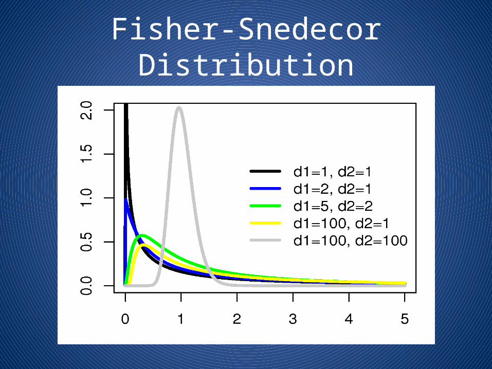
Fisher-Snedecor Distribution
F Test
• Null hypothesis: • Given df1 and df2, and F value, • Determine if corresponding probability is
within acceptable distribution region
Issues of ANOVA
• Indicates some group difference• Does not reveal which two groups differ• Needs other tests to identify specific group
difference– Hypothetical comparisons Contrast – No Hypothetical comparisons Post Hoc
• ANOVA has been replaced by multiple regressions, which can also be replaced by General Linear Modeling (GLM)
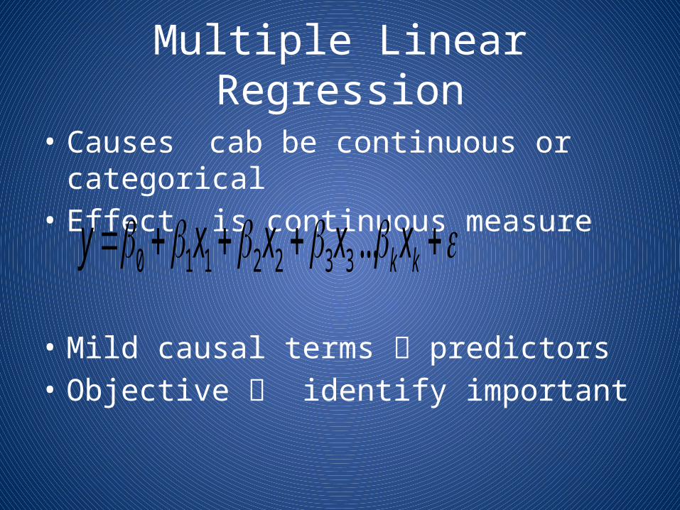
Multiple Linear Regression
• Causes cab be continuous or categorical • Effect is continuous measure
• Mild causal terms predictors• Objective identify important
0 1 1 2 2 3 3... k ky x x x x
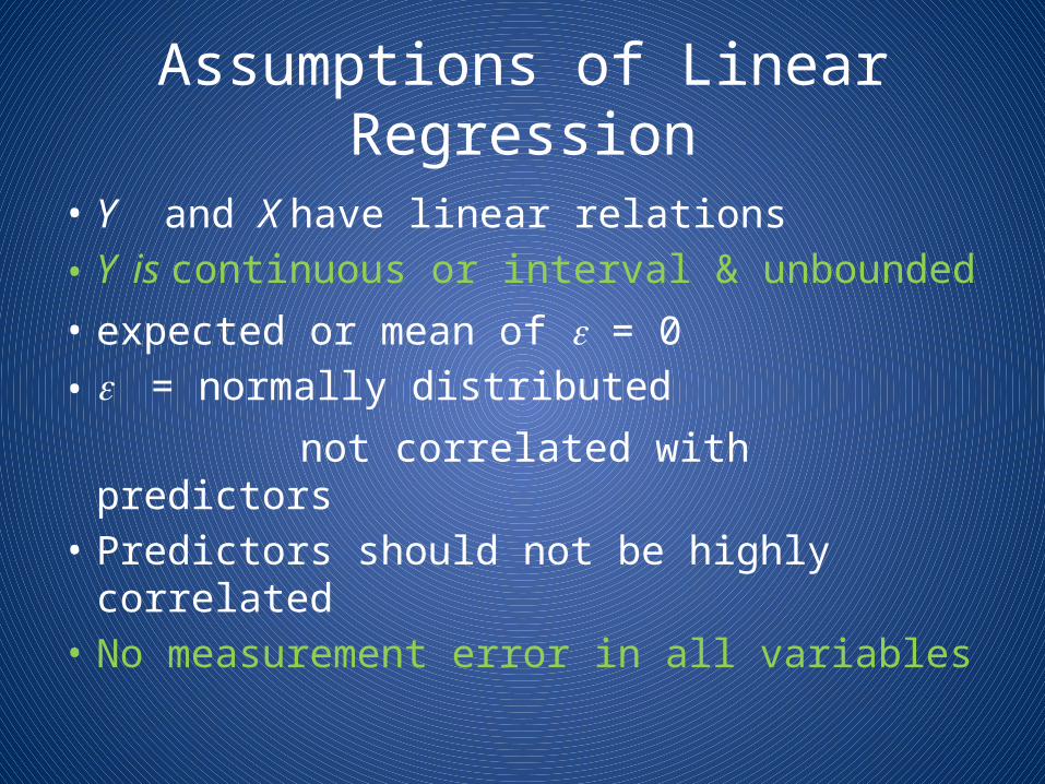
Assumptions of Linear Regression
• Y and X have linear relations • Y is continuous or interval & unbounded• expected or mean of = 0 • = normally distributed
not correlated with predictors• Predictors should not be highly correlated• No measurement error in all variables
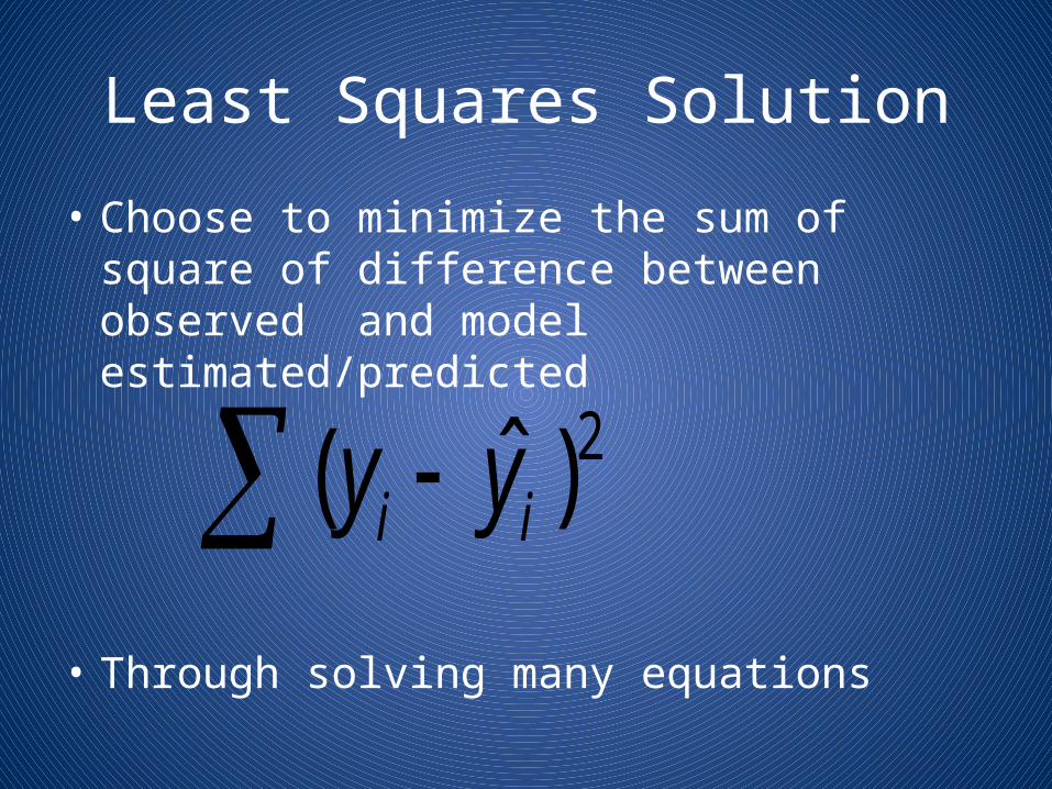
Least Squares Solution
• Choose to minimize the sum of square of difference between observed and model estimated/predicted
• Through solving many equations
2ˆ( )i iy y
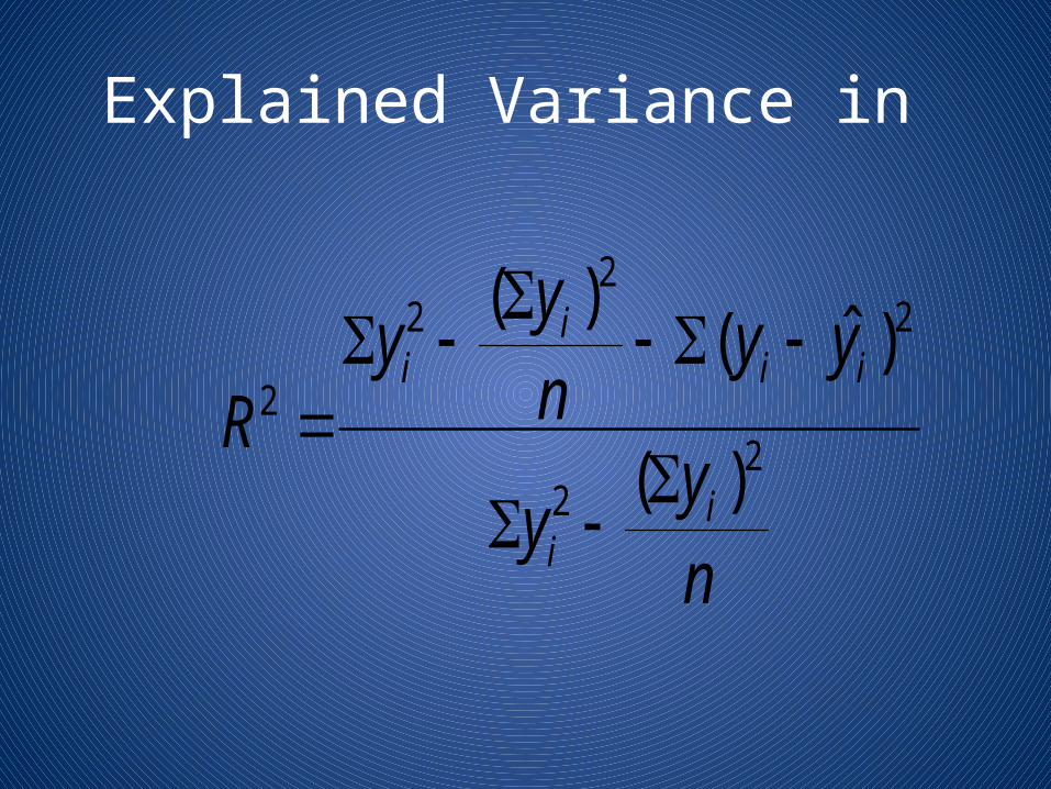
Explained Variance in
22 2
22
2
( )ˆ( )
( )
ii i i
ii
yy y y
nRy
yn
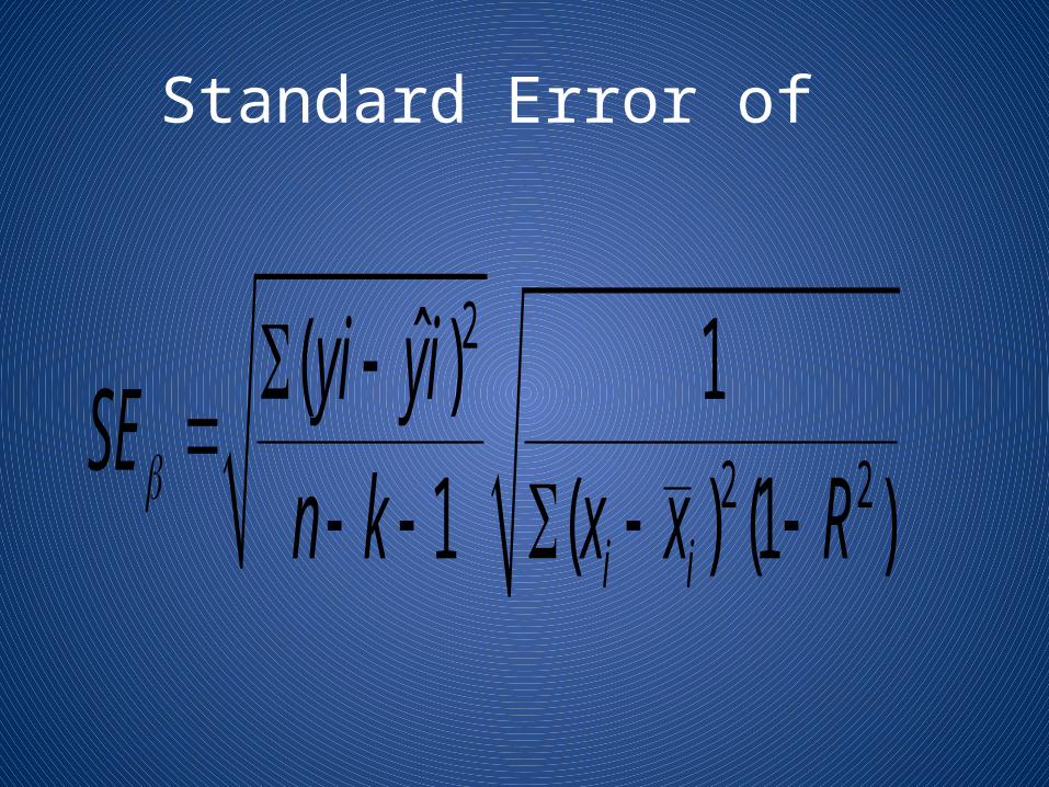
Standard Error of
2
2 2
ˆ( ) 1
1 ( ) (1 )i i
yi yiSE
n k x x R
T Test significant of
• t = / SE• If t > a critical value & p <.05 • Then is significantly different from zero
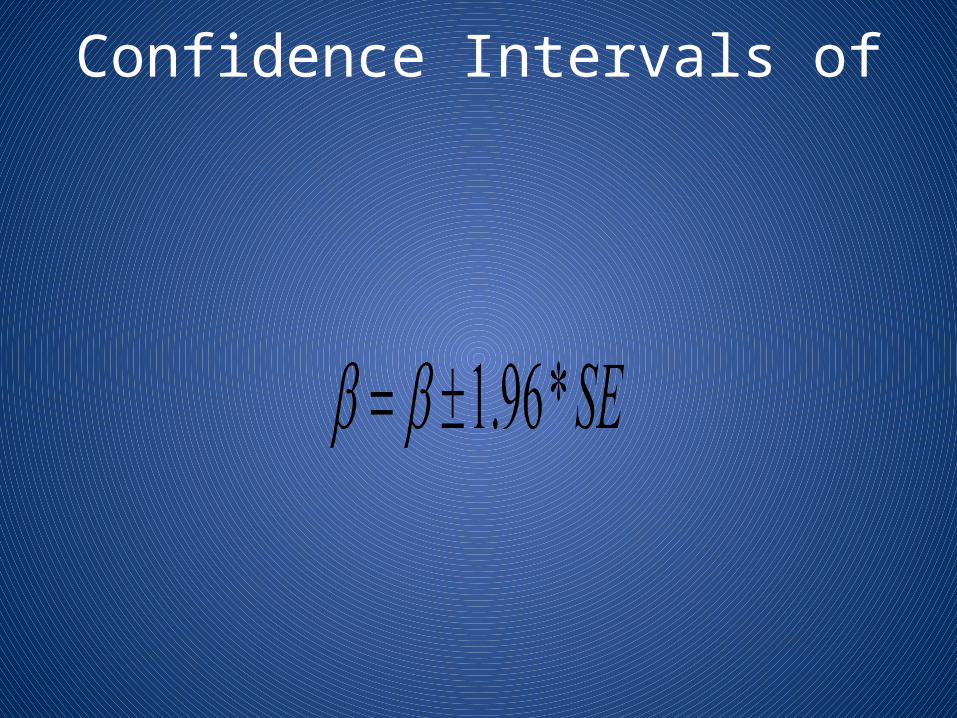
Confidence Intervals of
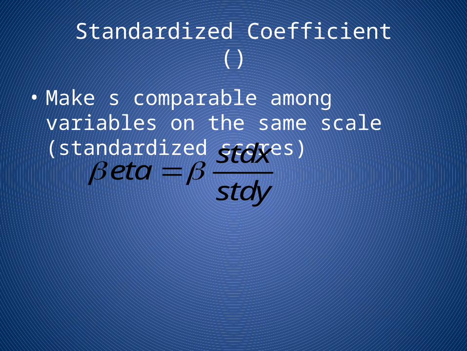
Standardized Coefficient()
• Make s comparable among variables on the same scale (standardized scores)
stdxeta
stdy
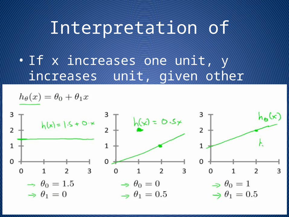
Interpretation of
• If x increases one unit, y increases unit, given other values of X
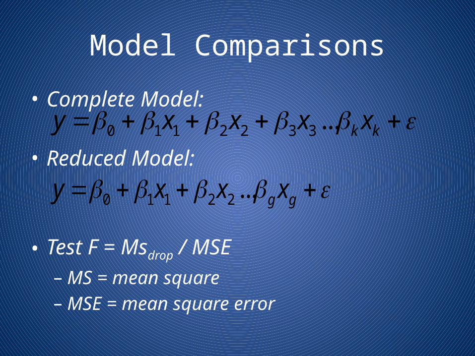
Model Comparisons
• Complete Model:
• Reduced Model:
• Test F = Msdrop / MSE– MS = mean square– MSE = mean square error
0 1 1 2 2 3 3... k ky x x x x
0 1 1 2 2... g gy x x x
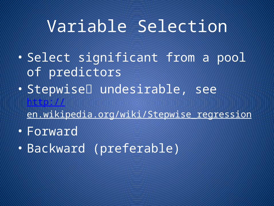
Variable Selection
• Select significant from a pool of predictors• Stepwise undesirable, see http://
en.wikipedia.org/wiki/Stepwise_regression
• Forward • Backward (preferable)
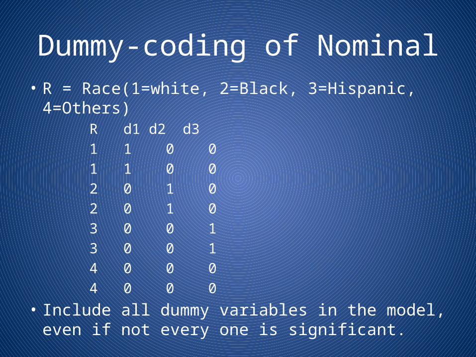
Dummy-coding of Nominal • R = Race(1=white, 2=Black, 3=Hispanic, 4=Others)
R d1 d2 d3 1 1 0 0 1 1 0 0 2 0 1 0 2 0 1 0 3 0 0 1 3 0 0 1 4 0 0 0 4 0 0 0
• Include all dummy variables in the model, even if not every one is significant.
Interaction
• Create a product term X2X3
• Include X2 and X3 even effects are not significant
• Interpret interaction effect: X2 effect depends on the level of X3.
0 1 1 2 2 3 3 4 2 3... k ky x x x x x x
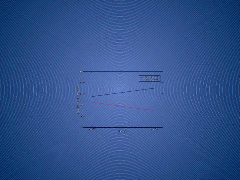
Plotting Interaction
• Write out model with main and interaction effects,
• Use standardized coefficient• Plug in some plausible numbers of interacting
variables and calculate y• Use one X for X dimension and Y value for the Y
dimension• See examples http://
frank.itlab.us/datamodel/node104.html
Diagnostic
• Linear relation of predicted and observed (plotting
• Collinearity • Outliers• Normality of residuals (save residual as new
variable)
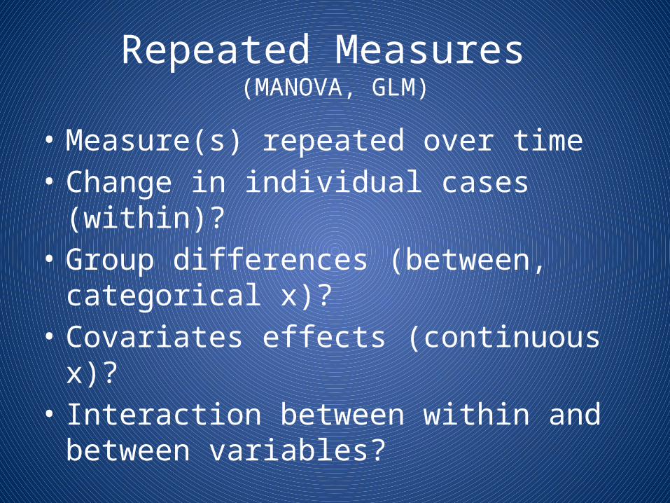
Repeated Measures (MANOVA, GLM)
• Measure(s) repeated over time • Change in individual cases (within)?• Group differences (between, categorical x)?• Covariates effects (continuous x)? • Interaction between within and between
variables?
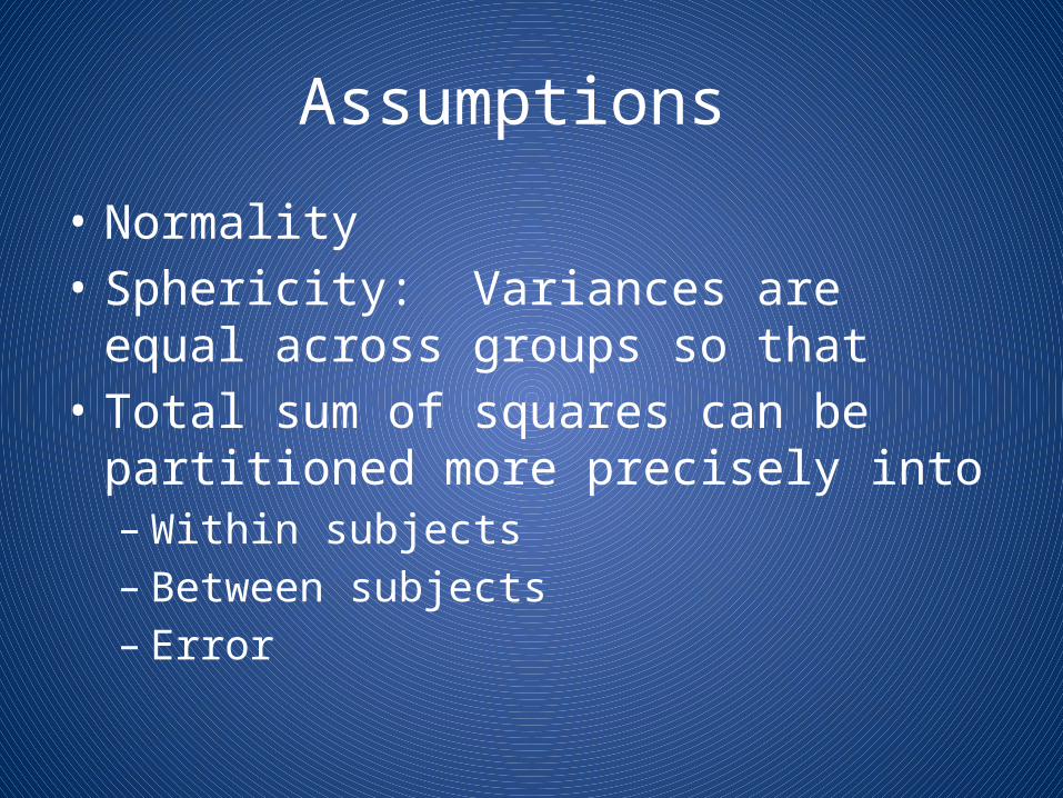
Assumptions
• Normality• Sphericity: Variances are equal across groups
so that • Total sum of squares can be partitioned more
precisely into – Within subjects– Between subjects– Error
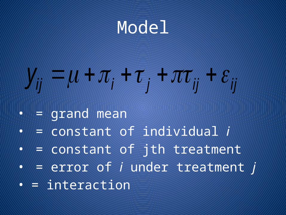
Model
• = grand mean• = constant of individual i• = constant of jth treatment• = error of i under treatment j• = interaction
ij i j ij ijy
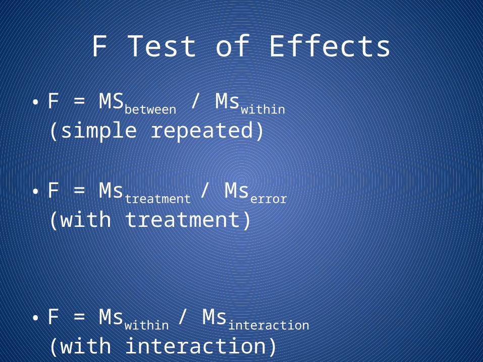
F Test of Effects
• F = MSbetween / Mswithin (simple repeated)
• F = Mstreatment / Mserror (with treatment)
• F = Mswithin / Msinteraction (with interaction)
Four Types Sum-Squares
• Type I balanced design• Type II adjusting for other effects • Type III no empty cell unbalanced design• Type VI empty cells
Exercise
• http://www.ats.ucla.edu/stat/spss/seminars/Repeated_Measures/default.htm
• Copy data to spss syntax window, select and run
• Run Repeated measures GLM

![Σύντομο Εγχειρίδιο SPSS 16 - psych.uoa.grroussosp/stats/Manual_SPSS16.pdf · Σύντομο Εγχειρίδιο SPSS 16.0 [3] Δυο λόγια εισαγωγικά](https://static.fdocument.org/doc/165x107/5bdb1b3f09d3f2d0098e03ac/-spss-16-psychuoagr-roussospstatsmanual.jpg)