Spectral problems on Riemannian manifolds - Universit© Joseph

1/53

Spectral problems on Riemannian manifolds


Pierre Bérard

Université Joseph Fourier - Grenoble

geometrias géométriesIMPA, April 13-15,2009

2/53

Spectral problems on Riemannian manifoldsIntroduction to the spectrum

Introduction to the spectrum

Let (M, g) be a compact Riemannian manifold (possibly withboundary). We consider the Laplacian on M, acting on functions,

∆g (f ) = δg (df ),

where δg is the divergence operator on 1-forms.

The divergence of a 1-form ω is given by

δg (ω) =n∑

j=1(Dg

Ejω)(Ej) =

n∑j=1

[Ej · ω(Ej)− ω(Dg

EjEj)],

where Ejnj=1 a local orthonormal frame.

3/53


In a local coordinate system xjnj=1, the Laplacian is given by

∆f = − 1vg (x)

n∑i ,j=1

∂

∂xi(vg (x)gĳ(x)

∂f∂xj

),

where(gĳ(x)

)is the inverse matrix

(gĳ(x)

)−1, the

gĳ(x) = g(∂

∂xi,∂

∂xj) are the coefficients of the Riemannian metric

in the local coordinates, and vg (x) =(Det(gĳ(x))

)1/2.

In local coordinates, the Riemannian measure dvg on (M, g) isgiven by

dvg = vg (x) dx1 . . . dxn.

4/53


We are interested in the eigenvalue problem for the Laplacian on(M, g), i.e. in finding the pairs (λ, u), where λ is a (real) numberand u a non-zero function, such that

∆u = λu

and, when M has a boundary ∂M, u|∂M = 0 (Dirichlet eigenvalueproblem).

We have the following theorem.

5/53


TheoremLet (M, g) be a compact Riemannian manifold. Then there exist asequence λ1 < λ2 ≤ . . . ≤ λk ≤ . . . of non-negative real numberswith finite multiplicities, and an L2(M, dvg )-orthonormal basisϕ1, ϕ2, . . . , ϕk , . . . of real C∞ functions such that ∆ϕj = λjϕj ,and ϕj |∂M = 0 if M has a boundary.

The set σ(M, g) = λ1, λ2, . . . , λk , . . . is called the spectrum ofthe Riemannian manifold (M, g) (Dirichlet spectrum, if M has aboundary). This is a Riemannian invariant (i.e. two isometricRiemannian manifolds have the same spectrum).

6/53


The main questions addressed by spectral geometry are thefollowing.

I Given a compact Riemannian manifold (M, g), can onedescribe σ(M, g) ?

I What information on σ(M, g) can one draw from geometricinformation on (M, g) ?

I What geometric information on (M, g) can one draw fromσ(M, g) ?

By information on σ(M, g), we mean bounds on the eigenvalues,their asymptotic behaviour, etc .

By information on (M, g), we mean bounds on curvature, on thevolume, on the diameter, etc .

7/53


Given (M, g), describe σ(M, g). Two examples.

I Flat tori. Let Γ be a lattice in Rn, Γ? the dual lattice and letTΓ = Rn/Γ be the corresponding flat torus. Then,

σ(TΓ) = 4π2‖γ?‖2 | γ? ∈ Γ?,

with associated eigenfunctions (Vol(TΓ))−1/2e2iπ〈γ?,x〉.I Round spheres. Let S2 be the unit sphere in R3, with induced

metric. Then,

σ(S2) = k(k + 1), with multiplicity 2k + 1 | k ∈ N.

The associated eigenfunctions are the restrictions to thesphere of harmonic homogeneous polynomials in R3.

8/53

Spectral problems on Riemannian manifoldsHeat kernel

Heat kernel

As an introduction to Gérard Besson’s lectures, I will first discusssome results obtained using the heat equation.

Let (M, g) be a closed (i.e. compact without boundary)n-dimensional Riemannian manifold.

We are interested in solving the Cauchy problem for the heatequation,

∂u∂t (t, x) + ∆xu(t, x) = 0u(0, x) = f (x)

where f is a given continuous function on M.

9/53

Spectral problems on Riemannian manifoldsHeat kernel

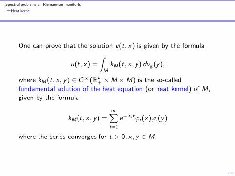
One can prove that the solution u(t, x) is given by the formula

u(t, x) =

∫MkM(t, x , y) dvg (y),

where kM(t, x , y) ∈ C∞(R•+ ×M ×M) is the so-calledfundamental solution of the heat equation (or heat kernel) of M,given by the formula

kM(t, x , y) =∞∑

i=1e−λi tϕi (x)ϕi (y)

where the series converges for t > 0, x , y ∈ M.

10/53

Spectral problems on Riemannian manifoldsHeat kernel, proofs

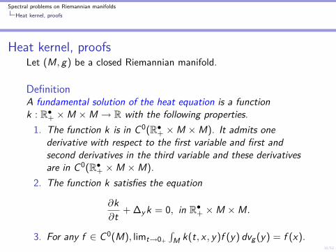
Heat kernel, proofsLet (M, g) be a closed Riemannian manifold.

DefinitionA fundamental solution of the heat equation is a functionk : R•+ ×M ×M → R with the following properties.1. The function k is in C0(R•+ ×M ×M). It admits one

derivative with respect to the first variable and first andsecond derivatives in the third variable and these derivativesare in C0(R•+ ×M ×M).

2. The function k satisfies the equation

∂k∂t + ∆yk = 0, in R•+ ×M ×M.

3. For any f ∈ C0(M), limt→0+

∫M k(t, x , y)f (y) dvg (y) = f (x).

11/53


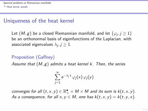
Uniqueness of the heat kernel

Let (M, g) be a closed Riemannian manifold, and let ϕj , j ≥ 1be an orthonormal basis of eigenfunctions of the Laplacian, withassociated eigenvalues λj , j ≥ 1.

Proposition (Gaffney)Assume that (M, g) admits a heat kernel k. Then, the series

∞∑j=1

e−λj t ϕj(x)ϕj(y)

converges for all (t, x , y) ∈ R•+ ×M ×M and its sum is k(t, x , y).As a consequence, for all x , y ∈ M, one has k(t, x , y) = k(t, y , x).

12/53


CorollaryThe series

∑∞j=1 e−λj t converges for all t > 0 and its sum is equal

to∫

M k(t, x , x) dvg (x).

13/53


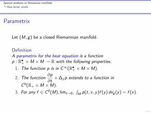
Parametrix

Let (M, g) be a closed Riemannian manifold.

DefinitionA parametrix for the heat equation is a functionp : R•+ ×M ×M → R with the following properties.1. The function p is in C∞(R•+ ×M ×M).

2. The function ∂p∂t + ∆yp extends to a function in

C0(R+ ×M ×M).

3. For any f ∈ C0(M), limt→0+

∫M p(t, x , y)f (y) dvg (y) = f (x).

14/53


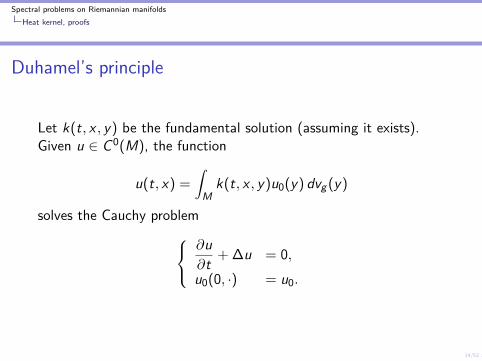
Duhamel’s principle

Let k(t, x , y) be the fundamental solution (assuming it exists).Given u ∈ C0(M), the function

u(t, x) =

∫Mk(t, x , y)u0(y) dvg (y)

solves the Cauchy problem∂u∂t + ∆u = 0,u0(0, ·) = u0.

15/53


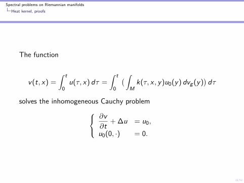
The function

v(t, x) =

∫ t

0u(τ, x) dτ =

∫ t

0

( ∫Mk(τ, x , y)u0(y) dvg (y)

)dτ

solves the inhomogeneous Cauchy problem∂v∂t + ∆u = u0,

u0(0, ·) = 0.

16/53


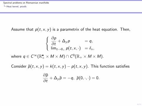
Assume that p(t, x , y) is a parametrix of the heat equation. Then,∂p∂t + ∆yp = q,limt→0+ p(t, x , ·) = δx ,

where q ∈ C∞(R•+ ×M ×M) ∩ C0(R+ ×M ×M).

Consider p(t, x , y) = k(t, x , y)− p(t, x , y). This function satisfies

∂p∂t + ∆y p = −q, p(0, ·, ·) = 0.

17/53


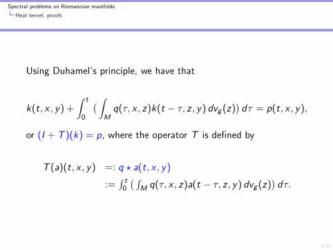
Using Duhamel’s principle, we have that

k(t, x , y) +

∫ t

0

( ∫Mq(τ, x , z)k(t − τ, z , y) dvg (z)

)dτ = p(t, x , y),

or (I + T )(k) = p, where the operator T is defined by

T (a)(t, x , y) =: q ? a(t, x , y)

:=∫ t

0( ∫

M q(τ, x , z)a(t − τ, z , y) dvg (z))dτ.

18/53


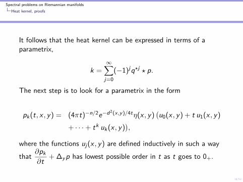
It follows that the heat kernel can be expressed in terms of aparametrix,

k =∞∑

j=0(−1)jq?j ? p.

The next step is to look for a parametrix in the form

pk(t, x , y) = (4πt)−n/2e−d2(x ,y)/4tη(x , y)(u0(x , y) + t u1(x , y)

+ · · ·+ tk uk(x , y)),

where the functions uj(x , y) are defined inductively in such a way

that ∂pk∂t + ∆yp has lowest possible order in t as t goes to 0+.

19/53


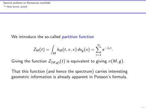
We introduce the so-called partition function

ZM(t) =

∫MkM(t, x , x) dvg (x) =

∞∑i=1

e−λi t .

Giving the function Z(M,g)(t) is equivalent to giving σ(M, g).

That this function (and hence the spectrum) carries interestinggeometric information is already apparent in Poisson’s formula.

20/53

Spectral problems on Riemannian manifoldsAsymptotic formulas

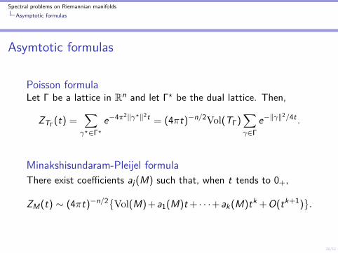
Asymtotic formulas

Poisson formulaLet Γ be a lattice in Rn and let Γ? be the dual lattice. Then,

ZTΓ(t) =

∑γ?∈Γ?

e−4π2‖γ?‖2t = (4πt)−n/2Vol(TΓ)∑γ∈Γ

e−‖γ‖2/4t .

Minakshisundaram-Pleĳel formulaThere exist coefficients aj(M) such that, when t tends to 0+,

ZM(t) ∼ (4πt)−n/2Vol(M) +a1(M)t + · · ·+ak(M)tk +O(tk+1).

21/53

Spectral problems on Riemannian manifoldsAsymptotic formulas

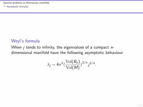
Weyl’s formulaWhen j tends to infinity, the eigenvalues of a compact n-dimensional manifold have the following asymptotic behaviour

λj ∼ 4π2(Vol(Bn)

Vol(M)

)2/n j2/n.

22/53

Spectral problems on Riemannian manifoldsEmbedding Riemannian manifolds by their heat kernel

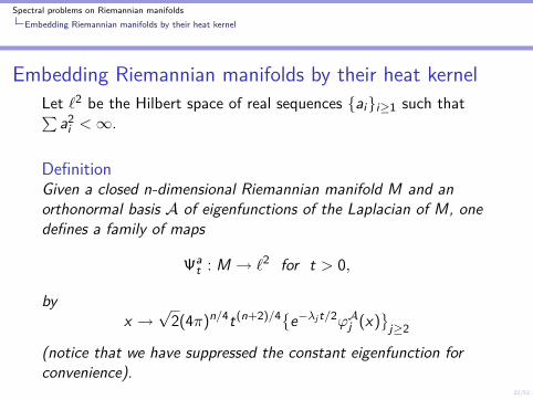
Embedding Riemannian manifolds by their heat kernelLet `2 be the Hilbert space of real sequences aii≥1 such that∑

a2i <∞.

DefinitionGiven a closed n-dimensional Riemannian manifold M and anorthonormal basis A of eigenfunctions of the Laplacian of M, onedefines a family of maps

Ψat : M → `2 for t > 0,

byx →

√2(4π)n/4t(n+2)/4e−λj t/2ϕAj (x)

j≥2

(notice that we have suppressed the constant eigenfunction forconvenience).

23/53


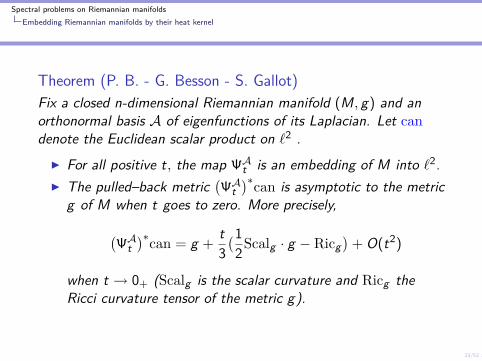
Theorem (P. B. - G. Besson - S. Gallot)Fix a closed n-dimensional Riemannian manifold (M, g) and anorthonormal basis A of eigenfunctions of its Laplacian. Let candenote the Euclidean scalar product on `2 .

I For all positive t, the map ΨAt is an embedding of M into `2.I The pulled–back metric

(ΨAt)∗can is asymptotic to the metric

g of M when t goes to zero. More precisely,

(ΨAt)∗can = g +

t3(12Scalg · g − Ricg

)+ O(t2)

when t → 0+ (Scalg is the scalar curvature and Ricg theRicci curvature tensor of the metric g).

24/53


An application

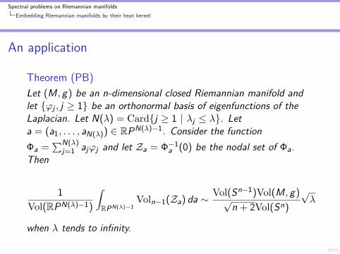
Theorem (PB)Let (M, g) be an n-dimensional closed Riemannian manifold andlet ϕj , j ≥ 1 be an orthonormal basis of eigenfunctions of theLaplacian. Let N(λ) = Cardj ≥ 1 | λj ≤ λ. Leta = (a1, . . . , aN(λ)) ∈ RPN(λ)−1. Consider the functionΦa =

∑N(λ)j=1 ajϕj and let Za = Φ−1

a (0) be the nodal set of Φa.Then

1Vol(RPN(λ)−1)

∫RPN(λ)−1

Voln−1(Za) da ∼ Vol(Sn−1)Vol(M, g)√n + 2Vol(Sn)

√λ

when λ tends to infinity.

25/53

Spectral problems on Riemannian manifoldsLower bounds on the eigenvalues

Lower bounds on the eigenvalues

Theorem (P.B. - G. Besson - S. Gallot)Let (M, g) be a closed n-dimensional Riemannian manifold. Definermin(M) = infRic(u, u) | u ∈ UM and let d(M) be the diameterof M. Assume that (M, g) satisfies rmin(M)d(M)2 ≥ (n − 1)εα2

for some ε ∈ −1, 0, 1 and some positive number α. Then, thereexists a real number R = a(n, ε, α)d(M), such that

Vol(M)kM(t, x , x) ≤ ZSn(1)(t/R2).

26/53


As a consequence of the previous theorem, we have the followingestimates for the eigenvalues and eigenfunctions of a closedn-dimensional Riemannian manifold (M, g) such thatRicg ≥ (n − 1)kg and d(M) ≤ D.

There exist explicit constants A(n, k,D) and B(n, k,D) such that λj(M, g) ≥ A(n, k,D) j2/n

Vol(M, g)∑λj≤λ ϕ

2j (x) ≤ B(n, k,D)λn/2.

27/53


Generalized Faber-Krahn inequality

Theorem (P. B. - G. Besson - S. Gallot)Let (M, g) be a closed n-dimensional Riemannian manifold suchthat rmin(M)d(M)2 ≥ (n − 1)εα2 for some ε ∈ −1, 0, 1 andsome positive number α. Then, there exists a real numberb(n, ε, α), such that

λ2(M, g) ≥ b(n, ε, α)d(M)−2.

28/53

Spectral problems on Riemannian manifoldsAnother embedding

Another embedding

We define another embedding of a closed n-dimensionalRiemannian manifold (M, g). Given some t > 0 and anorthonormal basis A of eigenfunctions of the Laplacian, let

IAt (x) = √

Vol(M) e−λj t/2 ϕAj (x)j≥2.

We also introduce the set

Mn,k,D =

(M, g)| dimM = n,Ricg ≥ (n − 1)kg ,Diam(M) ≤ D

of closed Riemannian manifolds.

29/53

Spectral problems on Riemannian manifoldsAnother embedding

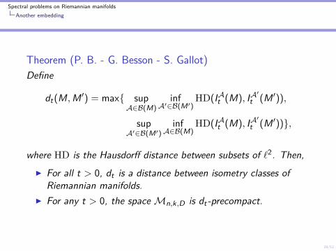
Theorem (P. B. - G. Besson - S. Gallot)Define

dt(M,M ′) = max supA∈B(M)

infA′∈B(M′)

HD(IAt (M), IA′t (M ′)),

supA′∈B(M′)

infA∈B(M)

HD(IAt (M), IA′t (M ′)),

where HD is the Hausdorff distance between subsets of `2. Then,I For all t > 0, dt is a distance between isometry classes of

Riemannian manifolds.I For any t > 0, the spaceMn,k,D is dt-precompact.

30/53

Spectral problems on Riemannian manifoldsVariational method and applications

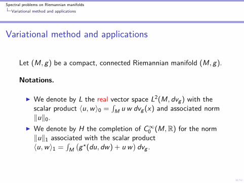
Variational method and applications

Let (M, g) be a compact, connected Riemannian manifold (M, g).

Notations.

I We denote by L the real vector space L2(M, dvg ) with thescalar product 〈u,w〉0 =

∫M u w dvg (x) and associated norm

‖u‖0.I We denote by H the completion of C∞0 (M,R) for the norm‖u‖1 associated with the scalar product〈u,w〉1 =

∫M(g?(du, dw) + u w

)dvg .

31/53

Spectral problems on Riemannian manifoldsVariational method and applications

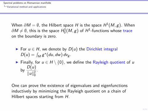
When ∂M = ∅, the Hilbert space H is the space H1(M, g). When∂M 6= ∅, this is the space H1

0 (M, g) of H1-functions whose traceon the boundary is zero.

I For u ∈ H, we denote by D(u) the Dirichlet integralD(u) =

∫M g?(du, dw) dvg .

I Finally, for u ∈ H \ 0, we define the Rayleigh quotient of u

by D(u)

‖u‖20.

One can prove the existence of eigenvalues and eigenfunctionsinductively by minimizing the Rayleigh quotient on a chain ofHilbert spaces starting from H.

32/53

Spectral problems on Riemannian manifoldsVariational method, proofs

Variational method, proofs

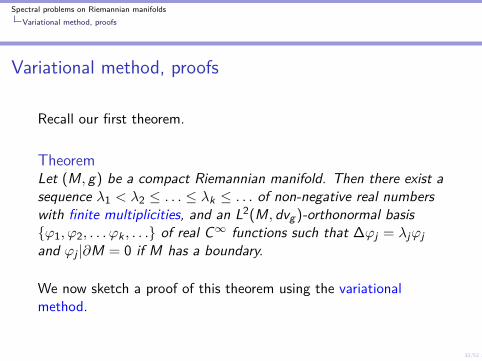
Recall our first theorem.

TheoremLet (M, g) be a compact Riemannian manifold. Then there exist asequence λ1 < λ2 ≤ . . . ≤ λk ≤ . . . of non-negative real numberswith finite multiplicities, and an L2(M, dvg )-orthonormal basisϕ1, ϕ2, . . . ϕk , . . . of real C∞ functions such that ∆ϕj = λjϕjand ϕj |∂M = 0 if M has a boundary.

We now sketch a proof of this theorem using the variationalmethod.

33/53


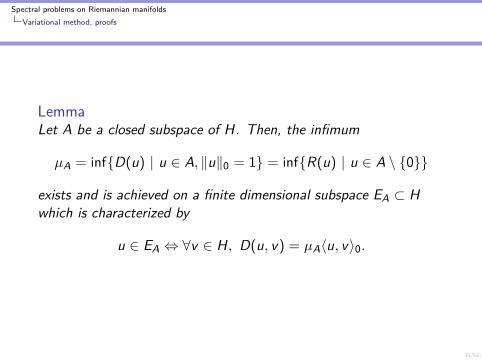
LemmaLet A be a closed subspace of H. Then, the infimum

µA = infD(u) | u ∈ A, ‖u‖0 = 1 = infR(u) | u ∈ A \ 0

exists and is achieved on a finite dimensional subspace EA ⊂ Hwhich is characterized by

u ∈ EA ⇔ ∀v ∈ H, D(u, v) = µA〈u, v〉0.

34/53


I The first eigenvalue is obtained by choosing A = H in theprevious lemma.

I Higher eigenvalues.I Other statements.

35/53


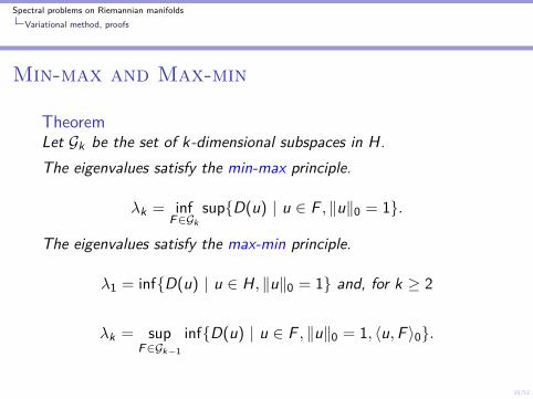
Min-max and Max-min

TheoremLet Gk be the set of k-dimensional subspaces in H.The eigenvalues satisfy the min-max principle.

λk = infF∈Gk

supD(u) | u ∈ F , ‖u‖0 = 1.

The eigenvalues satisfy the max-min principle.

λ1 = infD(u) | u ∈ H, ‖u‖0 = 1 and, for k ≥ 2

λk = supF∈Gk−1

infD(u) | u ∈ F , ‖u‖0 = 1, 〈u,F 〉0.

36/53


The least eigenvalue has a remarkable property. Any eigenfunctionassociated with λ1 does not vanish in the interior of M, thecorresponding eigenspace E1 has dimension 1, any eigenfuctionwhich does not vanish in the interior of M must be associated withthe least eigenvalue λ1.

37/53


Monotonicity principle

PropositionLet (M, g) be a Riemannian manifold and let Ω1 ⊂ Ω2 ⊂ M betwo relatively compact domains. Then

λD1 (Ω1) ≥ λD

1 (Ω2)

and strict inequality holds if the interior of Ω2 \ Ω1 is not empty.

38/53


Courant’s nodal domain theorem

TheoremLet u be an eigenfunction associated with the k-th eigenvalue.Then the number of nodal domains of u (i.e. of connectedcomponents of M \ u−1(0)) is at most k.

39/53


Eigenvalue comparison theorems

Theorem (S.Y. Cheng)Let (M, g) be any complete n-dimensional Riemannian manifoldsuch that Ricg ≥ (n − 1)kg. Then, for any x ∈ M and any R > 0,one has

λD1 (B(x ,R)) ≤ λD

1 (Bk(R)),

where Bk(R) denotes a ball with radius R in the simply-connectedn-dimensional model manifold with constant sectional curvature k.Furthermore, equality holds if and only if B(x ,R) is isometric toBk(R).

40/53


Theorem (S.Y. Cheng, M. Gromov)Let (M, g) be a closed n-dimensional Riemannian manifold suchthat Ricg ≥ (n − 1)kg. Let λ(k, ε) = λD

1 (Bk(ε)). Then, for allε > 0 and all j ≤ Vol(M)/Vol(Bk(2ε), λj ≤ λ(k, ε). In particular,there exists a constant C(n, k) such that

λj ≺ C(n, k)( jVol(M)

)2/n

when j tends to infinity.

Note that this estimate is coherent with Weyl’s asymptoticestimate.

41/53

Spectral problems on Riemannian manifoldsGeometric operators

Geometric operators

We have so far only considered the Laplacian on a closedRiemannian manifold. One can consider other interestinggeometric operators. Of particular interest is the Jacobi operatorassociated with the second variation of the area of minimal orconstant mean curvature hypersurfaces.

Let Mn # Mn+1 be a complete minimal orientable hypersurfaceimmersed into some Riemannian manifold M. Let NM be a unitnormal field along the immersion and let AM be the associatedsecond fundamental form. The Jacobi operator of the immersion isthe operator

JM = ∆M −(Ric(NM ,NM) + ‖AM‖2

).

42/53

Spectral problems on Riemannian manifoldsGeometric operators

Let λD1 (JM ,Ω) denote the least eigenvalue of the operator JM with

Dirichlet boundary conditions in Ω.

We say that the domain Ω is stable if λD1 (JM ,Ω) > 0 and weakly

stable if λD1 (JM ,Ω) ≥ 0.

The index of the domain Ω is the number of negative eigenvaluesof the operator JM in Ω with Dirichlet boundary condition.

43/53

Spectral problems on Riemannian manifoldsPositivity and applications

Positivity and applications

Theorem (I. Glazman / D. Fischer-Colbrie - R. Schoen)Let (M, g) be a complete Riemannian manifold and let q : M → Rbe a smooth function. For a relatively compact domain Ω ⊂ M, letλ1(Ω) be the least eigenvalue of the operator ∆ + q in Ω, withDirichlet boundary condition. The following assertions areequivalent.1. For all Ω b M, λ1(Ω) ≥ 0.2. For all Ω b M, λ1(Ω) > 0.3. There exists a positive function u on M such that

∆u + qu = 0.

44/53


Complete metrics on the unit disk

Theorem (D. Fischer-Colbrie – R. Schoen)Let (D, g) be the unit disk equiped with a metric g = µgeconformal to the Euclidean metric. Let K and ∆ denoterespectively the Gauss curvature and the Laplacian for the metric g(then 2K = ∆ lnµ).

If g is complete, then for any a ≥ 1, there is no positive solution ofthe equation (∆ + aK )f = 0 on D.

45/53


As a matter of fact, one has the following result (which has beenimproved by Ph. Castillon).

PropositionLet g = µge a complete conformal metric on the unit disk D.Then, there exists some numer 0 ≤ a0(g) < 1 such that

I for a ≤ a0, there exist no positive solution to (∆ + aK )f = 0on D,

I for a > a0, there exists a positive solution to (∆ + aK )f = 0on D.

46/53


CorollaryLet g be a complete conformal metric on the unit disk D. Fora ≥ 1 (a constant) and for p ≥ 0 (a function on D), there exist nopositive solution to (∆ + aK )f = pf .

47/53


Stable minimal surfaces in R3

Theorem (M. do Carmo - C. Peng / D. Fischer-Colbrie -R. Schoen)The only complete oriented stable minimal surface in R3 is theplane.

48/53


Jacobi fields

Let JM be the Jacobi operator of a minimal hypersurface M # M.A Jacobi field is a function u on M such that JM(u) = 0.

The geometry provides natural Jacobi fields. Indeed, we have thefollowing properties.

1. Let K be a Killing field in M. Then the functionuK = g(K,NM) is a Jacobi field on M.

2. Let ψa : M # M be a family of minimal immersions. Thenthe function va = g(dψa

da ,NM) is a Jacobi field on M.

49/53


Catenoïds in R3

Part of the proof of the positivity theorem can be restated as thefollowing corollary.

CorollaryLet Ω be any bounded open domain. Assume that there exists apositive function u on Ω such that (∆ + q)u = 0. Then,λ1(Ω) ≥ 0.

50/53


As an application, we can prove Lindelöf’s theorem for catenoïds inR3.

TheoremOne can characterize the maximal rotation-invariant stable domainsof the catenoids as generated by the arcs of the catenary whoseend-points have tangents meeting on the axis of the catenary. Inparticular, the half vertical catenoïd x2 + y2 = cosh2(z), z ≥ 0 is amaximal weakly stable rotation invariant domain.

Observe that the catenoïd x2 + y2 = cosh2(z) has index 1.

51/53


Generalizations

The same analysis can be applied to catenoids in H2 × R or in H3

and to their higher dimensional analogues, with the occurence ofinteresting phenomena. (work in progress PB - R. Sá Earp).

52/53


I would like to take this opportunity to thank IMPA for theirsupport and for hosting the main part of this event,and to thank the sponsors: Programme ARCUS Brésil (RégionRhône-Alpes – MAE), CNRS, IMPA, Université Joseph Fourier.

53/53


Thank you for your attention.

[email protected]

Spectral problems on Riemannian manifolds - Universit© Joseph

Documents

Transcript of Spectral problems on Riemannian manifolds - Universit© Joseph