
Get - Institute of Computer Engineering - Technische Universit¤t Wien
117
DISSERTATION Distributed Computing in the Presence of Bounded Asynchrony ausgef¨ uhrt zum Zwecke der Erlangung des akademischen Grades eines Doktors der technischen Wissenschaften unter der Leitung von Univ.Prof. Dr. Ulrich Schmid Inst.-Nr. E182/2 Institut f¨ ur Technische Informatik Embedded Computing Systems eingereicht an der Technischen Universit¨ at Wien Fakult¨ at f¨ ur Informatik von Dipl.-Ing. Josef Widder Matr.-Nr. 9625114 Meidlgasse 41/4/4 A-1110 Wien Europ¨ aische Union Wien, im Mai 2004
Transcript of Get - Institute of Computer Engineering - Technische Universit¤t Wien

DISSERTATION
Distributed Computing in the Presence of Bounded
Asynchrony
ausgefuhrt zum Zwecke der Erlangung des akademischen Gradeseines Doktors der technischen Wissenschaften
unter der Leitung von
Univ.Prof. Dr. Ulrich Schmid
Inst.-Nr. E182/2
Institut fur Technische InformatikEmbedded Computing Systems
eingereicht an der Technischen Universitat WienFakultat fur Informatik
von
Dipl.-Ing. Josef Widder
Matr.-Nr. 9625114
Meidlgasse 41/4/4A-1110 Wien
Europaische Union
Wien, im Mai 2004

i
Verteilte Algorithmen unter eingeschrankter Asynchronitat
Diese Dissertation untersucht verschiedene Aspekte des Θ-Modells, einem zeitfreienSystemmodell fur verteilte Systeme. Die zugrunde liegende Annahme ist die Existenzeines begrenzten Verhaltnisses der Ubertragungsdauern von Nachrichten die gleichzeitigunterwegs sind. Das Modell wurde von Le Lann und Schmid eingefuhrt, die zeigten,dass das fundamentale consensus Problem in ihm eine Losung besitzt.
Der erste Teil dieser Dissertation beschaftigt sich mit einer Neudefinition des Mod-ells basierend auf zwei Modellen. Als erstes das system model, das ein sehr flexi-bles Zeitverhalten modelliert und daher eine hohe Abdeckung moglicher Zustande vonrealen Netzwerken hat. Das zweite ist das computational model, das der ursprunglichenDefinition entspricht. Weiters wird gezeigt, dass die beiden Modelle gleich stark sind,dh. Probleme die eine Losung in einem Modell haben, haben auch eine im anderen.
Der zweite große Abschnitt beschaftigt sich mit Algorithmen und deren Verhaltenim Θ-Modell. Der grundlegende Algorithmus dient zur Uhrensynchronisation; auf ihmbasierend werden dann andere Algorithmen aufgebaut. In diesem Teil wird auch mittelsstrongly dependent decision problem gezeigt, dass das Θ-Modell bezuglich Losbarkeitvon Problemen zu den synchronen gezahlt werden muss, obwohl es keine obere Grenzevon Ubertragungsdauern voraussetzt.
Der dritte und letzte Abschnitt beschaftigt sich mit dem Problemkreis Netzwerk-initialisierung (booting). In der Theorie wird meist uber dieses Problem hinweg gese-hen, wahrscheinlich weil einfache Annahmen uber das Zeitverhalten getroffen werdenkonnen, die dieses Problem einfach “weg definieren”. Da in dieser Dissertation zeitfreieModelle und Algorithmen untersucht werden, sind solche Annahmen nicht zulassig,weil darauf basierende Losungen nicht mehr als zeitfrei bezeichnet werden konnen.Wie auch im zweiten Abschnitt beginnen wir mit Uhrensynchronisation in der Ini-tialisierungsphase und stellen dann Losungen von anderen Problemen vor, die daraufbasieren.

ii
iii
Distributed Computing in the Presence of BoundedAsynchrony
This thesis investigates various aspects of the Θ-Model. The Θ-Model is a time freemodel of distributed systems which assumes that end-to-end delays of the fastest andslowest messages over the network are correlated. This relation is expressed by givingan upper bound Θ on the ratio of longest and shortest transmission times of messageswhich are simultaneously in transit. The model was introduced by Le Lann and Schmid,who showed that the Θ-Model is sufficiently strong to solve the fundamental yet nottrivial problem of consensus. Their innovative results left room for improvement in thedefinition of the Θ-Model and raised some questions, including the amount of synchronyin the model and related to it what kind of problems have solution in it.
The first part of this thesis is dedicated to a refinement of the original definition ofthe Θ-Model. This is achieved by distinguishing two different models: The first one isthe system model, which is very flexible regarding the timing of the described system.It should reach very high assumption coverage—the probability that the assumptionsmade in a model hold in real systems. The second model is the computational model,which is similar to the original definition of the Θ-Model. After that, we show thatthese two models are equivalent with respect to expressiveness. It hence follows thatexisting results, which rely upon the original definition of the Θ-Model, are valid inthe novel system model as well.
The next major part introduces several algorithms and analyzes their behavior whenexecuted in the Θ-Model. The basic algorithm is a clock synchronization algorithmwhereupon several other algorithms—e.g. implementation of the perfect failure detec-tor and atomic commitment—are devised. This part also gives an answer to the ques-tion of the amount of synchrony in the model. Using the strongly dependent decisionproblem—which is sort of a benchmark that separates synchronous from asynchronousmodels—it is shown that the Θ-Model must in fact be attributed as synchronous. Thisis quite surprising given that the system model does not stipulate an upper bound onmessage transmission delays.
The third part considers booting. The problem of system startup is often neglectedin distributed computing theory. We believe that this is due to the fact that whenreal systems are considered, timed semantics are usually employed, which allow sev-eral simplifications of the booting problem. Since we consider a time free model, theproblem of booting clock synchronization is particularly difficult because classic failureassumption (e.g. f < n/3) cannot be employed properly in the booting phase. Basedupon a clock synchronization algorithm that properly handles booting, we show howto adapt solutions to other problems in distributed computing such that they provide(some of) their properties during booting as well.

iv
Acknowledgments
I am grateful to my supervisor Ulrich Schmid who is the best teacher I ever had. Heprepares an open and fruitful environment that allows young people (like I still pretendto be) to deliver scientific work at a level that can persist in the strong internationalcompetition. I thank Mehdi Jazayeri for his valuable comments and suggestions whengrading this thesis. I am also grateful to Gerard Le Lann who invited me to work withhim at INRIA Rocquencourt for two months. During this stay I learned very much,not limited to predictability of distributed systems. Further I thank Martin Hutle forproof reading drafts of this thesis. His remarks helped me improving the presentationof the results. Discussions with him give me deeper insight into many challenges weare facing.
Ich danke meiner Mutter Edith Widder und meinen Großeltern fur das Schaffen einesfamiliaren Umfeldes das mir mein Studium so leicht gemacht hat. Dank auch an meineFreunde Andi, Josef, Martin, Migo, und Tobi.
In Erinnerung an meinen Vater Josef Widder.
Supported by the Austrian BM:vit FIT-IT project DCBA, project no. 808198.
v

vi
vii
Human nature is such that simple, easy to understand solutions are spontaneouslyfavoured (and selected). However, with distributed real-time applications, the questionis whether such an instinctive attitude is appropriate. . .
Gerard Le Lann

viii
Contents
1 Introduction 11.1 Motivation for this Thesis . . . . . . . . . . . . . . . . . . . . . . . . . 21.2 Road Map . . . . . . . . . . . . . . . . . . . . . . . . . . . . . . . . . . 31.3 Related Work . . . . . . . . . . . . . . . . . . . . . . . . . . . . . . . . 4
2 Modeling Distributed Real-Time Systems 52.1 Network of Queues . . . . . . . . . . . . . . . . . . . . . . . . . . . . . 52.2 Asynchronous Distributed Real-Time Systems . . . . . . . . . . . . . . 72.3 Suitable Models for Real-Time Systems . . . . . . . . . . . . . . . . . . 7
3 The Θ-Model for Distributed Real-Time Systems 113.1 Physical System . . . . . . . . . . . . . . . . . . . . . . . . . . . . . . . 11
3.1.1 Faults . . . . . . . . . . . . . . . . . . . . . . . . . . . . . . . . 113.1.2 Timing . . . . . . . . . . . . . . . . . . . . . . . . . . . . . . . . 12
3.2 System Model . . . . . . . . . . . . . . . . . . . . . . . . . . . . . . . . 123.3 Computational Model . . . . . . . . . . . . . . . . . . . . . . . . . . . 133.4 Equivalence of the Models . . . . . . . . . . . . . . . . . . . . . . . . . 143.5 Round Based Significant Uncertainty Ratio . . . . . . . . . . . . . . . . 15
3.5.1 Byzantine Faults . . . . . . . . . . . . . . . . . . . . . . . . . . 163.5.2 Crash Faults . . . . . . . . . . . . . . . . . . . . . . . . . . . . . 173.5.3 Clean-Crash Faults . . . . . . . . . . . . . . . . . . . . . . . . . 17
3.6 Related Work . . . . . . . . . . . . . . . . . . . . . . . . . . . . . . . . 17
4 The Θ-Model Compared to other System Models 194.1 Partial Synchrony . . . . . . . . . . . . . . . . . . . . . . . . . . . . . . 194.2 Semi-Synchrony . . . . . . . . . . . . . . . . . . . . . . . . . . . . . . . 214.3 The Archimedean Assumption . . . . . . . . . . . . . . . . . . . . . . . 22
5 Implementation Issues 235.1 Design Immersion . . . . . . . . . . . . . . . . . . . . . . . . . . . . . . 235.2 Assumption Coverage . . . . . . . . . . . . . . . . . . . . . . . . . . . . 235.3 Real-Time Scheduling . . . . . . . . . . . . . . . . . . . . . . . . . . . . 245.4 Experimental Results . . . . . . . . . . . . . . . . . . . . . . . . . . . . 245.5 Deterministic Ethernet . . . . . . . . . . . . . . . . . . . . . . . . . . . 255.6 Algorithms at Application Level . . . . . . . . . . . . . . . . . . . . . . 25
ix
x CONTENTS
5.7 Bounded Drift Clocks . . . . . . . . . . . . . . . . . . . . . . . . . . . . 26
6 Selected Algorithms in the Θ-Model 276.1 Clock Synchronization . . . . . . . . . . . . . . . . . . . . . . . . . . . 27
6.1.1 Byzantine Case . . . . . . . . . . . . . . . . . . . . . . . . . . . 286.1.2 Clock Synchronization Properties . . . . . . . . . . . . . . . . . 306.1.3 Restricted Failure Modes . . . . . . . . . . . . . . . . . . . . . . 33
6.2 Failure Detection . . . . . . . . . . . . . . . . . . . . . . . . . . . . . . 376.3 Synchrony of the Θ-Model . . . . . . . . . . . . . . . . . . . . . . . . . 39
6.3.1 The Strongly Dependent Decision Problem . . . . . . . . . . . . 406.3.2 Fault-Tolerant Broadcast . . . . . . . . . . . . . . . . . . . . . . 426.3.3 Simulating Lock-Step . . . . . . . . . . . . . . . . . . . . . . . . 44
6.4 Non-Blocking Atomic Commitment . . . . . . . . . . . . . . . . . . . . 466.4.1 Clean-Crash Faults . . . . . . . . . . . . . . . . . . . . . . . . . 476.4.2 Crashes . . . . . . . . . . . . . . . . . . . . . . . . . . . . . . . 49
6.5 Related Work . . . . . . . . . . . . . . . . . . . . . . . . . . . . . . . . 506.5.1 Clock Synchronization . . . . . . . . . . . . . . . . . . . . . . . 506.5.2 Unreliable Failure Detectors . . . . . . . . . . . . . . . . . . . . 516.5.3 Synchronizers . . . . . . . . . . . . . . . . . . . . . . . . . . . . 516.5.4 Non-Blocking Atomic Commit . . . . . . . . . . . . . . . . . . . 52
7 Booting Clock Synchronization 537.1 Perception Based Failure Model . . . . . . . . . . . . . . . . . . . . . . 54
7.1.1 Execution Model . . . . . . . . . . . . . . . . . . . . . . . . . . 547.1.2 Model of the Startup Phase . . . . . . . . . . . . . . . . . . . . 587.1.3 Physical Failure Model . . . . . . . . . . . . . . . . . . . . . . . 597.1.4 Perception Failure Model . . . . . . . . . . . . . . . . . . . . . . 60
7.2 The Algorithm . . . . . . . . . . . . . . . . . . . . . . . . . . . . . . . 657.3 Mapping to the Perception based Execution Model . . . . . . . . . . . 677.4 From Early to Degraded Mode . . . . . . . . . . . . . . . . . . . . . . . 687.5 From Degraded to Normal Mode . . . . . . . . . . . . . . . . . . . . . 747.6 Related Work . . . . . . . . . . . . . . . . . . . . . . . . . . . . . . . . 81
8 Booting Θ-Algorithms 838.1 Eventually Perfect Failure Detector . . . . . . . . . . . . . . . . . . . . 838.2 General Considerations . . . . . . . . . . . . . . . . . . . . . . . . . . . 858.3 Lock-Step . . . . . . . . . . . . . . . . . . . . . . . . . . . . . . . . . . 858.4 Atomic Multicast . . . . . . . . . . . . . . . . . . . . . . . . . . . . . . 878.5 Non-Blocking Atomic Commitment . . . . . . . . . . . . . . . . . . . . 89
9 Conclusions 919.1 Required Synchrony for Consensus . . . . . . . . . . . . . . . . . . . . 919.2 Clock Synchronization Implementation . . . . . . . . . . . . . . . . . . 929.3 Dependable Real-Time Systems . . . . . . . . . . . . . . . . . . . . . . 929.4 Outlook on Further Research Directions . . . . . . . . . . . . . . . . . 93
Chapter 1
Introduction
A distributed system consists of a collection of autonomous computers linked by anetwork such that these computers can coordinate their activities and share their re-sources. They employ distributed algorithms for this purpose which consist of multipleprocesses that are executed concurrently on the multiple processors. In order to exhaus-tively describe the system’s behavior it is usually necessary to analyze these algorithmsand prove their properties mathematically.
In sharp contrast to single computer systems, the fault of a single component doesnot necessarily lead to a failure of the whole system. Distributed algorithms shouldhence be able to tolerate a given number of faulty remote processes or links. (Thesenumbers must usually be derived statistically from hardware and software error prob-abilities.) Adding the notion of fault tolerance to distributed systems renders manyproblems extremely difficult to handle, however. Classic results even show that funda-mental problems like agreeing on a common value—consensus—is impossible in certainsettings; cp. the well known FLP result [42]. These settings include the type of faults(e.g. computers that crash or send faulty values, lossy communications) and—of evenmore interest—the timing of the system. The mentioned FLP result, for example,just refers to one possible crash fault and to asynchronous systems, i.e. systems wheremessage transmission and relative computer speeds are unbounded. Still: What kindof distributed systems really need such weak assumptions? Are there computers thatare infinitely fast compared to others or are there networks where failure free sendingof a message takes infinitely long? Since this is not the case, the assumption coverageof system models must be considered.
Models of distributed systems are formulated by simplifying the observed objectsand by describing their behavior by sets of rules. These abstractions are used to reasonformally about system properties. Assumption coverage is a measure of how well themodel fits the real target system. It is the probability that the assumptions in themodel hold in the system. Returning to the FLP model, its coverage regarding timingassumptions is 1 in every real system such that solutions to problems in asynchronoussystems can be transferred into all types of systems without decreasing coverage. Sincethere is no solution for agreement in asynchronous systems, however, additional as-sumptions (feasibility conditions) must be added in order to solve the problem. These
1
2 CHAPTER 1. INTRODUCTION
assumptions should be as weak as possible such that coverage can be maximized. Muchwork [29, 19] was devoted to this problem. Two major approaches can be distinguishedhere: (1) Adding synchrony and (2) adding information about failures. As a matter offact these approaches are related to each other since implementing (2) is possible onlyby (1); nevertheless (2) is addressed in literature very often since it is a smart way toencapsulate synchrony in the asynchronous world.
Synchrony can be added by assumptions which are made about the timing behaviorof a system or system components, e.g. bounds on message delays and computingspeeds. Regardless of how values for the timing are derived, the probability thatthey hold during real operation must always be considered strictly less than 1. If thegoal is maximizing assumption coverage, the means for achieving this is weakeningthe assumptions as far as possible while maintaining the solvability of the requiredproblems (under the given set of assumptions).
But lets now turn to a special property of distributed computing problems: Real-time requirements. Real-time problems arise in applications where not only correctresponses are required, but these responses also have to meet deadlines. In the real-time community exists a widespread believe nowadays that synchronous (timed) systemmodels are required in order to provide solutions to real-time problems. It should beclear by now that these solutions have the drawback that their assumption coverage isnecessarily smaller than those of time free models. Therefore approaches are requiredthat reconcile real-time and maximal coverage. Such an approach is the design im-mersion principle [65, 66] which just states: Take a time free solution and analyze it(using schedulability analysis) on a given system that employs optimal online schedul-ing algorithms. If this analysis reveals that the solution executed on the given systemmeets all its deadlines we have a real-time system. This approach is preferable since, inorder to maximize safety (nothing bad ever happens) and coverage, least assumptionsshould be made and synchrony should be introduced as late as possible during thedevelopment life cycle. More abstractly, when immersing a time free solution into areal distributed system, we say that the system’s timing properties emerge. Thus it ispossible to design time free real-time systems. This thesis is devoted to this branch ofresearch.
1.1 Motivation for this Thesis
As one possible timing model for time free real-time applications, Le Lann andSchmid [67, 68] introduced the Θ-Model. In this model, Θ is a measure of asynchronyin distributed systems; namely an upper bound on the ratio of the longest and shortestend-to-end message transmission times. To demonstrate its suitability for algorithmssolving asynchronous real-time distributed computing problems, a major task is todevise solutions to the most fundamental agreement problems like FD based consensus,atomic broadcast and atomic commitment.
Since the problem of handling system booting becomes difficult in asynchronous—i.e. time free—designs, as already discussed in [106], the behavior of the mentionedalgorithms will be explored during booting as well.
1.2. ROAD MAP 3
In addition, a refinement of the original Θ-Model is presented, which is particularlypromising in terms of assumption coverage. Explicit upper bounds are dismissed by justreferring to longest message transmission at some given point in time which effectivelyleads to time dependent bounds (i.e. that may vary over time). It is then shown that thenew definition of the model has the same expressive power than the original definitionsuch that existing results remain valid. Moreover, the analysis of algorithms may stillbe conducted in the simple to handle original model and “mechanically” translatedinto the weaker model.
We compare the Θ-Model to partially synchronous and semi-synchronous models,by opposing the respective assumptions and discussing their relation. We also comparetheir respective power by examining solutions to some specific distributed computingproblems, like the SDD problem.
1.2 Road Map
The remainder of this thesis is divided into three major parts: The Θ-Model, algo-rithms, and system booting.
It starts with Section 2 where properties of real systems are discussed and severalmodels are examined w.r.t. their suitability for describing those. Based upon theseresults, we introduce the Θ-Model in Section 3, where we provide two models: Thesystem model in Section 3.2 models the timing behavior of a distributed system withhigh coverage. The second model is an easy to handle computational model whichis introduced in Section 3.3. We will show that both models are equivalent regardingexpressive power such that results of the computational model can easily be transferredto the high coverage system model of Section 3.2. Since, by then, we have introducedthe model we are ready to compare it to other well known models in Section 4. InSection 5 we discuss several practical issues related to the Θ-Model.
The second major part can be found in Section 6 and is devoted to algorithms for theΘ-Model. We introduce fundamental building blocks first which are required by anyof our high-level algorithms, namely clock synchronization in Section 6.1 and perfectfailure detection (for solving consensus) in Section 6.2. Section 6.3 is devoted to themore theory related question of the degree of synchrony in the Θ-Model. To accomplishthis, a solution of the strongly dependent decision problem is given which shows thatthe Θ-Model is equivalent to synchronous models in this respect. Based upon thosefoundations we give an algorithm for atomic broadcast in Section 6.3.2 and a lock-stepsimulation in Section 6.3.3. This simulation allows to solve agreement problems evenin presence of the most severe type of faults, i.e. Byzantine faults. Since non-blockingatomic commitment is not reducible to consensus or atomic broadcast in asynchronoussystems, we finally give solutions to this problem in Section 6.4 as well.
It is usually (implicitly) assumed in distributed computing theory that all processesare initially up such that they do not miss messages sent by other correct processes. Intimed systems it is convenient to use information on time for booting the system – atthe cost of reduced coverage though. Since we consider time free algorithms we musthandle system booting in a time free manner. The third major part is hence devoted to
4 CHAPTER 1. INTRODUCTION
this problem: A solution to the pivotal clock synchronization algorithm that works alsoduring booting is presented in Section 7. This section also reviews the perception basedfailure model, which underlies the analysis of our clock synchronization algorithm.Booting in the context of other distributed algorithms is discussed in Section 8.
1.3 Related Work
The books by Coulouris et al. [23], Tanenbaum et al. [97] and the book edited byMullender [77] are good introductions into basic problems and concepts of distributedsystems. More related to the work that is presented here are the books by Lynch [71],Attiya and Welch [9] and Tel [98] as they concentrate on the theoretical aspects ofdistributed systems and algorithms. Basic principles of real-time systems are presentedin the books by Kopetz [59] and Verıssimo et al. [101].
This thesis focuses on the Θ-Model and its ability to solve real-time problems. Theresults presented here build upon the work by Le Lann and Schmid, who introducedthe Θ-Model as well as an implementation of the perfect failure detector [67] and dis-cussed its ability to maximize coverage [68]. Part of our results were/will be publishedin a number of papers: Clock synchronization algorithms that support booting arepresented in [106, 109]. Based on these algorithms, a refinement of the failure detectorimplementation is given in [108], which can be used during booting as well. For avariant of the Θ-Model, were the synchrony assumptions hold just after some possiblyunknown global stabilization time, a simulation for Byzantine consensus is presentedin [107]. In [55] two self-stabilizing failure detector implementations are devised. Therelation of the Θ-Model to real-time networks is examined in [52]: The timing behaviorof Θ-algorithms is observed when executed in an architecture built upon deterministicEthernet.
Chapter 2
Modeling Distributed Real-TimeSystems
Since any solution to a problem in distributed real-time computing is just as goodas its underlying model, a crucial part in the design of dependable real-time systemsis the choice of the right model. When choosing a model, several topics must beaddressed. First of all, one has to examine what to describe, i.e. the type of systems thedevised algorithms shall eventually be executed on. A suitable model should adequatelydescribe the core properties of those systems. Among those are queuing phenomenonsas discussed in Section 2.1, which severely affect the system timing.
The problems that have to be solved by the algorithms are obviously another impor-tant topic that must be addressed when choosing a model. We discuss novel applicationdomains for real-time systems in Section 2.2.
After this we shortly review existing approaches which aim at these novel applicationdomains in Section 2.3 and discuss whether these are suitable for the problems we wantto address.
2.1 Network of Queues
A message transmission over a network consists of local message preparation atthe sender, transmission over the link, and local receive computation at the receiver.This is of course an abstraction which hides away that messages go through variousqueues at the sender and receiver such that the sojourn times in queues—dependingon scheduling characteristics—must be considered as important part of the messagetransmission delay δ.
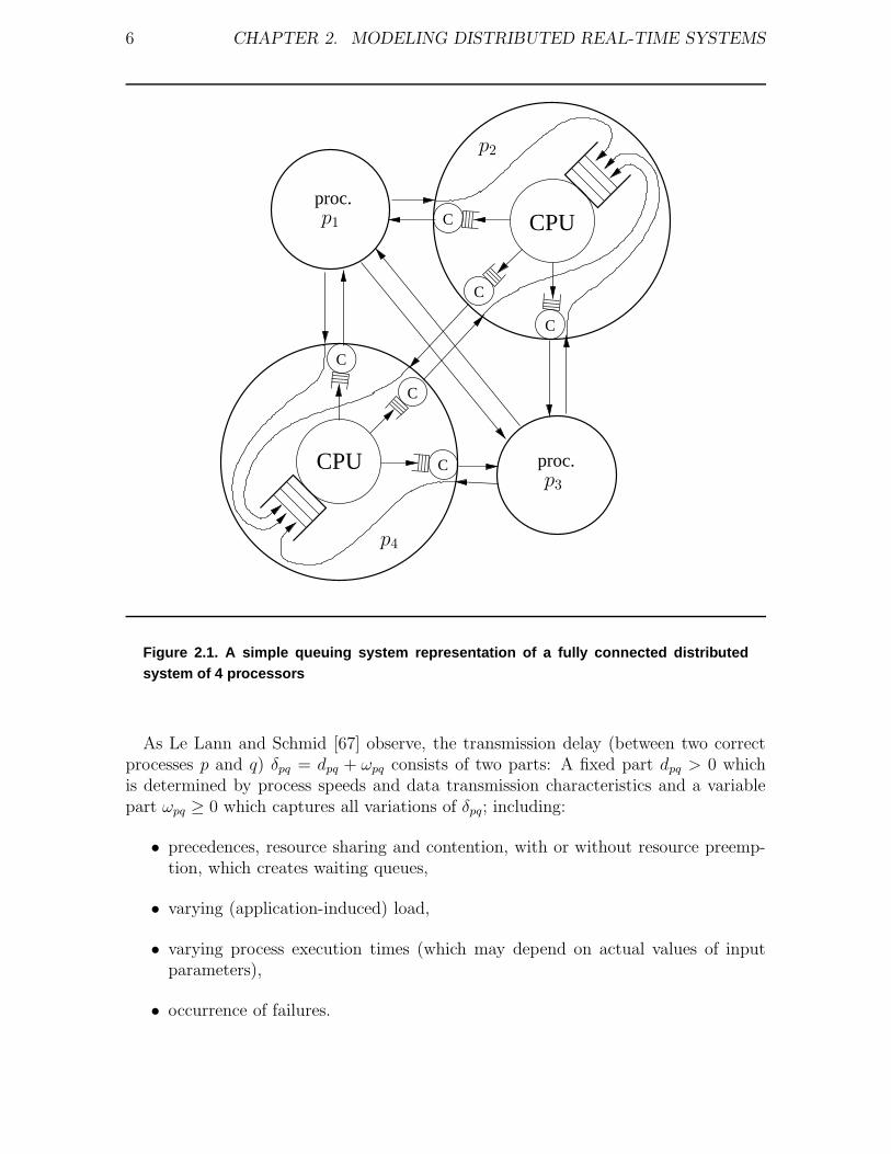
In Figure 2.1 it is depicted how a distributed system can be modeled as a network ofqueues. All messages that drop in over one of the n − 1 incoming links of a processormust eventually be processed by the single CPU. Every message that arrives while theCPU processes former ones must hence be put into the CPU queue for later processing.In addition, all messages produced by the CPU must be scheduled for transmission overevery outgoing link. Messages that find an outgoing link busy must hence be put intothe send queue of the link’s communication controller for later transmission.
5
6 CHAPTER 2. MODELING DISTRIBUTED REAL-TIME SYSTEMS
CPU
CPUC
C
C
C
C
C
proc.
proc.
p2
p3
p1
p4
Figure 2.1. A simple queuing system representation of a fully connected distributedsystem of 4 processors
As Le Lann and Schmid [67] observe, the transmission delay (between two correctprocesses p and q) δpq = dpq + ωpq consists of two parts: A fixed part dpq > 0 whichis determined by process speeds and data transmission characteristics and a variablepart ωpq ≥ 0 which captures all variations of δpq; including:
• precedences, resource sharing and contention, with or without resource preemp-tion, which creates waiting queues,
• varying (application-induced) load,
• varying process execution times (which may depend on actual values of inputparameters),
• occurrence of failures.
2.2. ASYNCHRONOUS DISTRIBUTED REAL-TIME SYSTEMS 7
Especially in networks with shared channel topologies (like Ethernet), these pointsdo not vary independently at different nodes. The shared channel makes it impossiblefor the adversary to slow down just some messages, and hence to violate some upperbound τ+ without slowing down all messages simultaneously. It follows that the lowerbound on messages delays τ− cannot be attained simultaneously during such periods.Hence, the Θ-Model (cp. Section 3) does not bound τ+ and τ− but just the ratio ofthese bounds Θ = τ+/τ−. Regarding coverage this is advantageous for systems wherethe smallest delays (τ−) are increased at least by c/Θ whenever the longest delays (τ+)increase by an amount of c: Obviously, Θ cannot be violated here.
2.2 Asynchronous Distributed Real-Time Systems
Recently, new application domains, like space, autonomy and artificial intelligenceetc. became targets for distributed real-time systems [56]. A peculiarity of thesenew applications is the timing behavior induced by the uncertainty regarding futureoperational environments. Requirements of such applications are hence different fromclassical application domains of real-time systems, like engine control or industrialautomation at machine level. These applications normally comprise very simple controltasks executed on dedicated processors with constant computation load and thereforepredictable timing behavior, such that synchronous timing models are suitable, i.e.have sufficiently large coverage (the probability that the assumptions in the modelhold during real operation).
For the above mentioned new application domains new system models must be de-vised since synchronous models of computation do not apply. One reason for this areuncertain environments: Consider long lived space borne applications, for example,where timing uncertainty is induced just by the unpredictable environment. Anothersource for asynchrony are intensive on demand computations. Choosing timing boundsfor normal operation according to rare computation requirements is costly and oftennot even required from a safety point of view. Finally using COTS (commercially ofthe shelf) components significantly reduces costs which opens new application domainsfor real-time systems. Unfortunately—due to pipelines, caches etc.—modern COTSprocessors do have quite unpredictable timing behavior. Therefore weaker models ofcomputation should be devised [51, 66] in order to increase the coverage.
2.3 Suitable Models for Real-Time Systems
We now shortly review what kinds of weak timing models have been devised by thedistributed computing community, and how suitable they are for real-time distributedapplications. It is very well known that, due to the fundamental FLP impossibilityresult [42], important agreement problems have no solution in the weakest timingmodel, i.e. pure asynchrony. Since our goal are models that are as weak as possible, wetake FLP as starting point and review what can be added to the asynchronous modelin order to solve agreement problems which are required as building blocks for mostreal-time control applications.
8 CHAPTER 2. MODELING DISTRIBUTED REAL-TIME SYSTEMS
Lets start with the most abstract approach taken by Chandra and Toueg [19], whointroduced the concept of failure detectors (FDs) and showed that even unreliable FDsare sufficient to solve consensus in asynchronous systems. We regard their contribu-tion as twofold. On one hand they formulated what kind of information on failures isrequired by processes in asynchronous environments in order to solve consensus. Sec-ond, FDs are time free constructs which hide synchrony assumptions. As shown byHermant and Le Lann [51], this second contribution can be employed very efficientlyin real-time systems by recognizing that implementing FDs can be done in lower net-work layers. As already exploited in many clock synchronization based application,lower level uncertainty is much smaller than application level uncertainty, i.e. clockscan be synchronized closer than it would be possible on application level (where theyare used). FD implementations can, similarly, be devised which detect failures fast,i.e. in shorter times than application level messages may travel in the worst case.
Nevertheless, FDs are abstract, time free constructs. For distributed real-time sys-tems we must guarantee that all deadlines are met, i.e. we have to model the synchronyof our system more explicitly. Note that we may still refer to FD based solutions, butwe have to give time bounds on failure detection times as well as on termination ofagreement algorithms. We therefore now discuss some timing models which are neithertotally asynchronous nor totally synchronous.
Dolev, Dwork and Stockmeyer [29] investigated how much synchronism has to beadded to asynchronous systems in order to solve consensus. They identified five syn-chrony parameters (processors, communication, message order, broadcast facilities andatomicity of actions) which can be varied into 32 different partially synchronous sys-tem models. For each of those, they investigated whether consensus is solvable or not.Solutions for consensus in such system models are given in the paper by Dwork, Lynchand Stockmeyer [37], where two sources for uncertainty—computational speed andtransmission times—are considered. They postulated ∆ as (unknown) upper boundon message delay (on the network) and Φ as upper bound on relative computationalspeeds. Although this model is weaker than the synchronous model, it has many hid-den assumptions which do not seem suitable for real-time applications. For exampledelivering of a set of message takes one step regardless how large this set is. This totallyignores timing uncertainty induced by different queuing schemes and varying networkload during operation. One step is required as well to send a message point-to-point.We believe—and argue this in more detail in Section 4.1 and Section 4.2—that suchmodeling is not suitable for real-time requirements since the hidden assumption aretoo restrictive for the targeted application domains.
As mentioned above, new application domains for real-time systems [56] triggeredsome more recent research on novel timing models. We will discuss two well knownapproaches here, namely the timed asynchronous distributed system model TA [24, 74]and the timely computing base model TCB [99, 100, 17].
The TA model assumes that during system operation there exist sufficiently longperiods during which no faults occur and liveness can be achieved. At first sightthis appears similar to the partial synchronous models [37] where it is assumed that,after some stabilization time, the system is synchronous. Partial synchronous models
2.3. SUITABLE MODELS FOR REAL-TIME SYSTEMS 9
describe systems where a known bound exists and eventually holds, however, whereas inTA some δ on the message delays is defined. How the value for δ is chosen is applicationdependent. One approach proposed in [24, 74] is that if the system should react withinD real-time units, and the protocol requires a message chain consisting of k messagesin order to react, then δ
∆= D/k should be chosen. From this definition follows the
definition of a timing fault, i.e. a message transmission that requires more than δ time.This is, in the best case, just a partial solution to a real-time problem. In fact δ is notan upper bound, but just some value for which it is assumed that “most” messages arefaster than δ. The solution of a real-time problem would require a guarantee that δholds sufficiently often, but no solution to this problem is given in [24, 74].
The TCB takes the same approach: Definition of timing properties. But here awhole subsystem, the timely computing base, is defined. Whenever the applicationrequires something to happen timely, the TCB is used (for e.g. message transmission,local timeout). A TCB is defined to be independent of the asynchronous part of thesystem (interposition). The TCB is protected from faults that could violate timing(shielding). And its complexity is such that verifiable mechanisms can be implemented(validation). The problem, however, is that the description of the TCB [99] doesnot provide “feasibility conditions” like how often it may be used to transmit timelymessages, while in the description of an example TCB implementation [17] it is arguedthat it cannot be overloaded since load can be controlled. Again, this is in the best casejust a partial solution to a real-time problem since deriving rules on message arrivalswould be required to ensure that the TCB is in fact timely. No such rules are presentedin [99, 100, 17].
Both, TA and TCB are timed system models, i.e. local information on time is usedto detect remote performance faults. The question arises whether this is required. It isoften argued that such faults have to be detected in order to take actions that preventhazards, i.e. to ensure safety. And it is believed that using local information on timeprovided by clocks is required to do so. The design immersion principle, introducedby Le Lann [51, 66] takes a different approach. The goals that have to be reached bya real-time system are safety, liveness, and timeliness. Distributed computing theorytells us that, for many problems, safety and liveness can be reached even in asyn-chronous systems, or at least in some sort of weak partial synchronous models. Designimmersion describes a system engineering process where a design is made based on theweakest synchrony assumptions possible and formally proved to meet safety require-ments (nothing bad ever happens) and liveness requirements (eventually somethinggood happens). Only after this, the solution is immersed into a real target proved (e.g.via scheduling analysis) to satisfy certain timeliness requirements in this target systemas well.
The advantage of this approach is increased coverage: It is more likely that safety andliveness hold in time free designs than in designs resting directly on the assumed timingproperties of the target system: Improved coverage means that there are system stateswhere the immersed solution still delivers some service while the direct solution doesnot. In order to investigate this we have to consider exceptional cases: Consider periodswhere the target system’s behavior deviates from the expected one, which cannot be

10 CHAPTER 2. MODELING DISTRIBUTED REAL-TIME SYSTEMS
ruled out as 100% coverage is impossible to reach, especially when missions with longoperation times in not completely predictable environments have to be considered.In such periods a design resting on weaker assumptions may still deliver safety andliveness, while just timeliness is lost. A design directly resting on the target systemmay lose safety and liveness along with timeliness. Note that in such periods it isimpossible for any solution to ensure timeliness, such that the best one can hope foris maintaining safety and liveness (properties which can be ensured even in purelyasynchronous systems according to distributed computing theory).
The question, however, arises what kind of weak models are suitable for designimmersion. There are two requirements for such systems: (1) important problems (likeconsensus) must have a solution in the model, (2) the model’s timing assumptions mustbe implementable in real systems, and the assumptions should even hold in cases wherethe system does not behave as expected (in order to improve coverage further). Webelieve that the Θ-Model which was introduced by Le Lann and Schmid [67], is wellsuited for modeling real-time distributed systems. Unlike other partially synchronousmodels, the Θ-Model is sufficiently strong to solve consensus and related problemseven in the absence of upper bounds on message transmission delays with links thatneed not provide FIFO (First-In First-Out) semantics. The apparent contradiction toFLP [42, 29] is resolved by replacing the upper bounds ∆ and Φ by an upper boundΘ on the ratio of longest and shortest end-to-end transmission times. Computationalspeeds and transmission times are hence put together into end-to-end delays, which isthe only duration which must adhere to our assumptions.
This kind of modeling has at least three important advantages: (1) for terminationtimes of real-time applications only the end-to-end delays are relevant such that re-garding anything else unnecessarily complicates analysis. (2) By modeling end-to-enddelays we are less restrictive regarding relative computational speeds and transmissiontimes: Only their sum must behave as expected such that a violation of either onedoes not necessarily lead to violation of our assumption. (3) Research results [68, 5]show that there exists a relation of upper and lower message transmission times inmany systems: If a network is in a high load or even an overload state it is clear thatupper message transmission times are larger than in low load periods. But in highload periods all messages must be queued at the network interfaces such that even thefastest transmissions become slower as well. In [52] we provide an example of how tobuild a system with a small value for Θ and how to prove timeliness properties of thissystem while executing time free algorithms.
Chapter 3
The Θ-Model for DistributedReal-Time Systems
After discussing the motivation for introducing new models we now formally define theobjects of the Θ-Model and their interrelationships.
3.1 Physical System
We consider a system of n distributed processes1 denoted as p, q, . . ., which commu-nicate through a reliable, error free and fully connected point-to-point network2. Weassume that a non-faulty receiver of a message knows the sender. This assumption alsoincludes that processes have distinct identifiers which can be ordered uniquely3. Thecommunication channels between processes need not provide FIFO transmission, andthere is no authentication service4.
3.1.1 Faults
The most fundamental algorithms (clock synchronization) of this thesis deal withByzantine nodes. In order do tolerate them we define the following threshold: Amongthe n processes there is a maximum of f < n/3 faulty ones. No assumption is madeon the behavior of Byzantine faulty processes.
Problems like non-blocking atomic commitment (Section 6.4), reliable broadcast(Section 6.3.2), or strongly dependent decision (Section 6.3.1) are traditionally studiedin the presence of crash respectively clean-crash faults only. By clean-crash fault wemean processes that do not crash in the middle of the execution of a statement. Werequire such behavior for statements like “send message to all” in order to ensure
1For conciseness we assume that every of the n processors in a system executes just one process.2A model where several classes of link failures [109, 68] are considered is employed later, in Section 7.3This assumption is required for atomic broadcast in Section 6.3.2 which requires that messages
are ordered according to process identifiers.4We do not consider authenticated algorithms since it is never guaranteed that malicious processes
cannot break the authentication scheme. By devising solutions without authentication, our correctnessproofs cannot be invalidated by this event.
11
12 CHAPTER 3. THE Θ-MODEL FOR DISTRIBUTED REAL-TIME SYSTEMS
consistent message transmissions5. Crash faulty processes on the other hand maycrash at any time. In the presence of clean-crash faults we require systems wheref < n. If crash faults are considered we require f < n/2. These numbers stem fromthe requirement to implement clock synchronization (compare Section 6.1.3).
In Section 7 we will use the perception based hybrid failure model [88] which in-corporates various types of process and link failures. The model is discussed there ingreater detail.
3.1.2 Timing
We consider time free algorithms, i.e. processes that do not have access to hardwareclocks or an external time base. Regarding timing behavior we distinguish two models:The system model described in Section 3.2 which describes a dynamic timing behaviorwith no upper bounds upon message transmission delays δ. The ratio of longest andshortest message delays of messages that are simultaneously in transit, however, isbounded. Such timing behavior renders the analysis of such systems very complicated.To simplify the analysis we therefore introduce our computational model in Section 3.3which just considers fixed but unknown upper and lower bounds on message transmis-sion delays. We then show in Section 3.4 that these two models are equivalent, i.e.algorithms that have been shown to satisfy their safety and liveness requirements inthe computational model also work in the system model.
Except the fundamental clock synchronization algorithm, all algorithms in this thesiswill have a priori knowledge of some integer Ξ which is a function of the uncertaintyratio Θ (read on).
Regarding system booting we assume throughout Section 6 that all correct processesare initially up and listening to the network. We will see in Section 7 and Section 8,however, how to get rid of this assumption in a time free manner.
3.2 System Model
Processes communicate by message passing. The time interval a message m is intransit consists of three parts: Local message preparation (includes queuing) at thesender, transmission over the link, and local receive computation (includes queuing)at the receiver. We denote tm
s the instant the preparation of message m starts. Theinstant the receive computation is finished is denoted as tm
r .In our system model we say that message m is in transit during the real-time interval
[tms , tmr ). We denote by δm = tmr − tms the end-to-end computational + transmissiondelay of message m sent from one correct process to another. Further let M(t) be theset of all messages between correct processes that are in transit at real-time t. Let τ−(t)be a lower envelope function on transmission delays of all messages that are in transitat real-time t, such that for any time t it holds that τ−(t) ≤ min(δm) for all m ∈ M(t)if |M(t)| > 0 and τ−(t) = 1 otherwise. We define for a fixed Θ ∈ IR, Θ ≥ 1 the upper
5Such behavior can usually be simulated in the presence of crash faults by reliable broadcast. Thisis discussed later in Section 6.3.2 and Section 6.4.2.
3.3. COMPUTATIONAL MODEL 13
envelope function τ+(t) ≤ Θτ−(t). At any time t it must hold that τ+(t) ≥ max(δm)for all m ∈ M(t) if |M(t)| > 0.
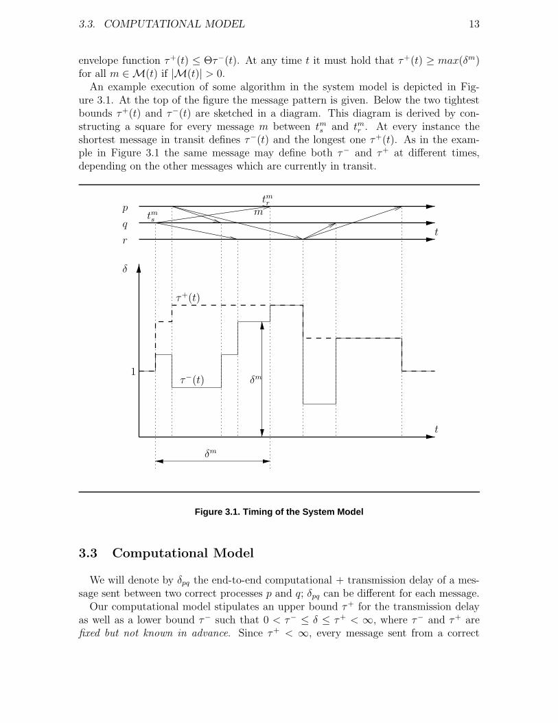
An example execution of some algorithm in the system model is depicted in Fig-ure 3.1. At the top of the figure the message pattern is given. Below the two tightestbounds τ+(t) and τ−(t) are sketched in a diagram. This diagram is derived by con-structing a square for every message m between tm
s and tmr . At every instance theshortest message in transit defines τ−(t) and the longest one τ+(t). As in the exam-ple in Figure 3.1 the same message may define both τ− and τ+ at different times,depending on the other messages which are currently in transit.
p
q
r
τ+(t)
τ−(t)
δ
t
t
1
tms
tmr
δm
δm
m
Figure 3.1. Timing of the System Model
3.3 Computational Model
We will denote by δpq the end-to-end computational + transmission delay of a mes-sage sent between two correct processes p and q; δpq can be different for each message.
Our computational model stipulates an upper bound τ+ for the transmission delayas well as a lower bound τ− such that 0 < τ− ≤ δ ≤ τ+ < ∞, where τ− and τ+ arefixed but not known in advance. Since τ+ < ∞, every message sent from a correct
14 CHAPTER 3. THE Θ-MODEL FOR DISTRIBUTED REAL-TIME SYSTEMS
process to another one is eventually received. Measures for the timing uncertaintyare the transmission delay uncertainty ε = τ+ − τ− and the transmission delay ratioΘ = τ+/τ−.
3.4 Equivalence of the Models
We now show the equivalence of our two models. We argue that an observer of thesystem which is equipped with a “real-time clock” whose timebase emerges from thesystem is not able to distinguish executions in the system model from executions inthe computational model.
Theorem 1 (Equivalence). The system model and the computational model have thesame expressive power.
Proof. Let us assume an omniscient observer in both systems who is equipped with aclock which provides him with observer-real-time, i.e. a time base that look to him likereal-time. More specifically, we assume that the observer-real-time t′ is constructed asa function of Newtonian time t in the following way:
t′ = β(t) =∫
1
τ−(t)dt. (3.1)
In the computational model, where τ−(t) = τ−, we hence get as time base β(t) =t/τ−+c, thus all correct message transmission delays take between 1 and Θ of observer-real-time here.
We now consider a message m between two correct processes in the system model.In order to get the measured value of the end-to-end delay we have to consider β(tm
r )−β(tms ). For any time t ∈ [tms , tmr ), we have tmr − tms ≥ τ−(t) ≥ tm
r−tm
s
Θ. By monotonicity
of integrals we get
1 ≤ β(tmr ) − β(tms ) =
tmr
∫
tms
dt
τ−(t)≤ (tmr − tms ) ·
Θ
tmr − tms= Θ.
Since both, the system and the computational model are time free, no action canoccur based on a timeout of a hardware clock etc. but only upon reception of a messageand upon the completion of processor startup:
• Processor startup. Since processes start at unpredictable times, the occurrencesof the very first action of every processor are completely unrelated in either model.
• Message reception. Apart from the very first action, all subsequent actions andhence messages sent by a correct process are direct responses to a received mes-sage.
When monitoring the execution of a distributed algorithm in system S using theappropriate observer-real-time clock, the observer cannot decide whether S adheres tothe computational or to the system model.
3.5. ROUND BASED SIGNIFICANT UNCERTAINTY RATIO 15
More informally one can argue about the equivalence when referring to the lengthof message chains: During the transmission of a (slow) message m, there cannot be aconcurrent causal message chain which has at least one (broadcast or receive) event incommon with m such that the chain consists of more than Θ messages during [tm
s , tmr ).Theorem 1 reveals that the system model which does not incorporate upper bounds
on message transmission times (given that Θ holds) can in fact be reduced to a partiallysynchronous model with fixed but unknown upper and lower time bounds. It is hencepossible to analyze distributed algorithms in the simple to handle computational modeland transfer the results regarding safety and liveness to the more “elastic” systemmodel.
Stating timeliness results in the context of real-time systems also requires specialcare: If the analysis in the computational model shows that some algorithm has arunning time depending on τ+, one has to be aware of the fact that these resultsmust be translated to the system model where we just have the function τ+(t). Theunderlying system’s timing behavior during some execution of our algorithm henceemerges to upper network layers. Assume t1 is the time when an execution startsaccording to observer-real-time base β, and t2 when it ends. The elapsed real-timeis then determined by ∆t = β−1(t2) − β−1(t1). When proving worst case responsetimes in real-time systems, however, the strict upper bound on τ+(t) of the consideredsystem must be considered during the late binding process. Only by carefully derivedupper bounds on message delays—by referring to the distributed real-time schedulingproblem— timeliness properties can be said to be properly achieved.
Remark The definition of τ−(t) = 1 in the case of no messages in transit was intro-duced in order to construct β(t) in the proof of Theorem 1 as an one-to-one mapping.It has no influence on bounds on durations of executions, and is only required duringinitialization of the algorithm (since we have no simultaneous start assumption). Afterinitialization there will always be messages in transit and our envelope functions aredefined in the natural way. One could also think of an extension of the Θ-Model thatallows local timeouts (e.g. to reduce traffic). Such timeouts must properly taken careof when analyzing worst case response times, however.
3.5 Round Based Significant Uncertainty Ratio
In this thesis we will only consider round based algorithms in the Θ-Model. Suchalgorithms are executed in asynchronous rounds, i.e. every correct process sends amessage for every round k. The transition to round k + 1 occurs when n− f messagesfor the current round are received. It will turn out that the uncertainty we have to dealwith does not stem from the ratio of message delays directly but rather from the ratioof the longest message delay and the shortest round switching intervals. The shortestround-switching interval τf, however, is not determined by only a single correct message.Rather it is determined by the sending time of the first message and the receive time ofthe n − f th message. In the worst case this is irrelevant since any message is boundedby τ−, and all could be sent simultaneously. From a practical point of view this is
16 CHAPTER 3. THE Θ-MODEL FOR DISTRIBUTED REAL-TIME SYSTEMS
very important, however. If one tries to establish an analytical expression for τ− onewould examine an idle system and the sending of a single message in this system—which could be a self reception as well. Obviously the receiver just has to deliver onemessage here. However, assuming that the receiver can process, say n − f messagesas fast as a single one is typically not valid in real systems. Choosing τf = τ− hencewould be overly conservative since round switching requires n − f messages, i.e. isdetermined by the n − f fastest message. In particular, in broadcast bus networksone cannot transmit two messages simultaneously over the bus, i.e. the n − f fastestmessages must be transmitted one after the other. The time for n − f messages to betransmitted in such networks is hence always larger than the best case time of sending asingle message in an idle system. Using τ− in the analysis would lead to over-valuationsof the significance of τ−.
Since we will consider several types of faults and hence different clock synchronizationalgorithms, the uncertainty ratio Θ used in our analysis will be slightly different fordifferent fault classes.
3.5.1 Byzantine Faults
In our round based algorithms, the transition to the next round occurs when n − fmessages for the current round have been received i.e. when at least n − 2f ≥ f + 1messages sent by correct processes have arrived. In our timing analysis, we will henceset τf equal to the transmission time of the n − 2f fastest correct message. Morespecifically, we will use τf as expression for the shortest time it may take to sendn − f messages from distinct processes to one receiver (end-to-end). This choice isadvantageous since τf need not be satisfied by all messages, but just by the n − 2ffastest one between two correct processes. Consequently, τ− will not show up in theanalytical expression for shortest round switching intervals explicitly, although of courseτf ≥ τ−. The system’s timing is therefore not violated even when up to f processescommit early timing failures, i.e. their messages are faster than τf. Let us formalizethis observation:
Definition 1 (Incoming Messages). For any correct process q, τ−q is the n − 2f
smallest δpq for all messages sent by correct processes p that enable an event at q. τf isdefined as the the smallest τ−
q of all correct processes q.
Lemma 1 (Sending Time). If a correct process receives messages from at least n−2fdistinct correct processes by time t, then at least one message was sent by time t − τf.
Proof. Follows from Definition 1.
Definition 2 (Significant Uncertainty Ratio). The smallest feasible value of theuncertainty ratio Θ is Ω = τ+/τf.
Remark Note that τf determines the time required for n− f messages to be receivedby a correct process. There are two possible approaches here. Assuming τf > τ− leadsto small values for Θ, and hence improved performance. This requires, however, that
3.6. RELATED WORK 17
all correct processes behave as expected regarding timing. Another approach, however,would consist of improving reliability, i.e. coverage. Setting τf = τ− we would allow upto f Byzantine faults and, additionally, f otherwise correct processes to commit earlytiming faults without violating the bound on the round-switching intervals.
3.5.2 Crash Faults
Asynchronous execution where just benign faults are considered are slightly different.We assume that processes are correct until they crash. Round switches will happenbased on the reception of n − f messages from correct (not yet crashed) processes.Hence τf can be defined similar to the Byzantine case by replacing n − 2f with n − fin Definition 1 and hence Lemma 1. Note carefully, however, that early timing faultsmust not happen here!
3.5.3 Clean-Crash Faults
Round switches will happen based upon the reception of message from n − f ≥ 1processes, thus τf = τ− must be considered. In many applications, however, f isconsiderably smaller than n. In such cases τf can be defined as in the crash fault case.
3.6 Related Work
The need for thinking about various types of synchrony started with the fundamentalpaper by Fischer, Lynch and Paterson [42] who showed that there is no deterministicalgorithm for asynchronous systems that solves consensus if just one process may crash.
Dolev, Dwork and Stockmeyer [29] investigated how much synchronism has to beadded to asynchronous systems in order to solve consensus. Dwork, Lynch and Stock-meyer [37] gave consensus algorithms for several kinds of partial synchrony. Theseresults are also presented in the book by Lynch [71]. More work on agreement underdiverse partially synchronous system models can be found in [8, 7, 81].
Chandra and Toueg [19] introduced the concept of unreliable failure detectors (FDs).Chandra, Hadzilacos, and Toueg [18] have shown the weakest type of unreliable FDsthat solves consensus. More related work on FDs can be found in Section 6.5.
Timed semantics and the failure detector approach are compared by Charron-Bost,Guerraoui and Schiper [21] who show that synchronous systems are strictly strongerthan asynchronous systems equipped with the perfect failure detector P.
In real-time systems research, however, asynchronous algorithms have almost neverbeen used. This is a consequence of the widespread believe that in order to build real-time applications timed algorithms have to be used [24, 100]. The design immersionprinciple (also referred to as late binding) by Le Lann [65, 66] has shown that thisbelieve is wrong! Hermant and Le Lann [51] have shown that it is possible to useasynchronous algorithms efficiently to solve real-time computing problems. Moreoverit is possible to show that implementations using late binding reach higher coverage.Regarding soft real-time systems there exists some work as well that deals with theusage of asynchronous algorithms [53].

18 CHAPTER 3. THE Θ-MODEL FOR DISTRIBUTED REAL-TIME SYSTEMS
Chapter 4
The Θ-Model Compared to otherSystem Models
Having introduced our Θ-Model in Section 3, we will now investigate the differenceswith respect to classic approaches on modeling the timing of distributed systems be-tween the two extrema lock-step synchrony and pure asynchrony. We consider herepartial synchrony [37], semi-synchrony [81], and the Archimedean assumption [103].
4.1 Partial Synchrony
In the Θ-Model we consider end-to-end delays, i.e. τ+(t) and τ−(t), whereas partiallysynchronous—denoted as ParSync—models [37] incorporate delays as follows:
∆ is the upper bound on message delays (not end-to-end)
Φ is the upper bound on the relative computational speeds.
When taking a closer look at the definition of Φ one finds that the time base ParSync-real-time is defined as the frequency of steps of the fastest process. Therefore at anyinstant in ParSync-real-time a process may take at most one step. Furthermore, anycorrect process must take at least one step when the fastest one makes Φ steps. Thishas two important implications: From the theoretical point of view, ParSync turns outto be a special case of the Θ-Model, i.e. the Θ-Model is strictly closer to asynchrony inthe hierarchy than ParSync. From the point of view of coverage, the ParSync modelturns out to have limited abilities to model real systems.
Lets start with the theoretical point of view. Bounded Φ means that no computa-tional step can be taken in 0 time. Regarding end-to-end delays (which are modeled inthe Θ-Model) ParSync models must have τ− > 0: At any time a process may take atmost one step where sending and receiving of some message cannot happen simulta-neously. However, any end-to-end delay must be measured in ParSync as the intervalbetween ”the time process p sends a message to q” and ”the time q sends its nextmessage” (in reaction to p’s). Since receive and send cannot happen at q at the sametime we get τ− ≥ 1.
19
20 CHAPTER 4. THE Θ-MODEL COMPARED TO OTHER SYSTEM MODELS
Bounded Φ also means that there exists a finite lower bound on process speeds,i.e. no process is infinitely slow. In conjunction with the bounded message delay thisimplies a bounded end-to-end delay τ+ as well.
To make a fair comparison of the synchrony assumptions of the Θ-Model andParSync, we have to examine the models more closely. In [37] ParSync comes intwo flavors:
ParSync.GST - ∆ is known, and holds from some global stabilization time on.
ParSync.Unknown - ∆ is unknown, and holds always.
From the existence of τ− > 0 and τ+ < ∞ we arrive at the conclusion that theΘ-Model and the ParSync model can be strictly ordered in hierarchy. For this we haveto consider two additional versions of the Θ-Model (note that, in this thesis, we willmostly stick to the ’classic’ Θ-Model when devising algorithms, since we are interestedin algorithms suitable for distributed real-time systems. Nevertheless, we will refer tothe other variants several times):
Θ.GST - some known Θ holds just from some global stabilization time on: We canemploy one of the algorithms presented later (Theorem 11) which implementsP. It follows that ParSync.GST is a special case of this model with fixed lowerand upper bounds on end-to-end delays that hold after GST.
Θ.Unknown - some unknown Θ always holds: We can update the timeout integerΞ in the FD implementation (compare Section 6.2) whenever a message from asuspected process drops in. Eventually Ξ will become the correct value. It followsthat ParSync.Unknown is a special case of this model with fixed lower and upperbounds on end-to-end delays.
These two findings imply that our algorithms could be run in ParSync models andwould work as expected. Therefore the Θ-Model fully includes ParSync and is hencestrictly closer to asynchrony.
As far as coverage of ParSync in real systems is concerned, we note that even theslowest process p must be able to receive a subset of the messages which were addedto its message buffer since its last step. The synchrony assumption, however, requiresthat it must receive a message m at the latest ∆ ParSync-real-time steps after m wasput into its in buffer. Lets construct a worst case scenario in this model: Let n − 1processes be fast and send, at every step, a message to the single slow process p. If onewants to implement the model in a real system, the duration of a step must be suchthat p can deliver (n− 1)Φ messages during a step. Otherwise the in-buffer of p couldnot be emptied at each step, such that it would require unbounded memory.
We believe that this modeling has some shortcomings: Fast and slow processesrequire the same amount of time for a step. When looking at queuing issues, it becomesobvious that the length of a step must depend on the time a slow process requires todeliver (n − 1)Φ messages. Therefore the performance of a fast process is limited
4.2. SEMI-SYNCHRONY 21
by the delivering speed of a slow one. Consequently, there exist a considerably largeτ− = 1ParSync in ParSync models, which is far away from being 0.
It follows that ParSync’s definition of computation speed has influence only on send-ing messages. For receiving messages a slow process and a fast one deliver the samenumber of messages during the same time interval. Just that a fast process deliverssome messages every instant and the slow one delivers many messages just every Φinstants. This is not a proper way of modeling slow process and clearly inferior to themodeling of end-to-end delays in the Θ-Model.
4.2 Semi-Synchrony
The usage of the term partial synchrony [37, 29] as described in Section 4.1has slightly changed in recent years. In literature models are called ParSync nowwhich where originally referred to as semi-synchronous (SemiSync), obviously since inSemiSync [80, 81, 8] there also exist Φ and ∆ (compare Section 4.1). There is, however,a slight difference: Since processes may deliver messages and send responses in zerotime, there does not exist some bounded τ− > 0 in this model. The absence of thissynchrony-enabling parameter is compensated by referring to bounded-drift local clocks(timers, hardware clocks, watchdogs etc.). The existence of some (possibly unknown)Φ and ∆ (and hence τ+) makes it possible to detect crashes based on approximatelocal information on the progress of real-time provided by local clocks.
We will later see in Section 5.7 that even the existence of local clocks does not help(w.r.t. increasing performance or number of solvable problems) in the Θ-Model. Thisis due to the fact that τ+(t) does not imply a strict upper bound on end-to-end delays.We now informally discuss this property by referring to SemiSync.
The way how clocks are used in SemiSync relies on the following property: Due tobounded Φ and ∆ and the existence of a bounded drift clock, a correct process’s clockticks at most some x times until some message from a correct process must arrive. Inthe Θ-Model, Φ and ∆—represented now by τ+(t)—vary over time, such that boundeddrift clocks are of no help.
We believe that SemiSync models do not exploit properly the inherent synchrony ofall real computer networks: Setting the lower bound to 0 is obviously a safe assumption,but real systems have lower bounds on message transmissions (due to the physicalimpossibility of transmitting and processing information in zero time).
From a theoretical viewpoint SemiSync is of course of highest interest since its lowerbounds on termination times apply to weaker models as well.
Non-technical Remark Before returning to more technical topics, lets have a lookat the aesthetics of the Θ-Model when compared SemiSync (and to ParSync): InSemiSync, times from different domains are compared: Message delays and clock fre-quencies. We believe that these two domains are totally independent, such that compar-ing them, in order to timeout processes is not an elegant solution. (Whether eleganceshould be left in the domain of tailors and shoemakers will not be discussed here.)Exploiting the inherent synchrony of the system (recall τ− > 0 in any real system) andcomparing (somehow) slow and fast messages is preferable from this viewpoint as well.
22 CHAPTER 4. THE Θ-MODEL COMPARED TO OTHER SYSTEM MODELS
4.3 The Archimedean Assumption
The Archimedean assumption was introduced by Vitanyi [102, 103] and limits adistributed systems asynchrony. It was employed in the context of message and timecomplexity bounds for distributed systems with realistic timing behavior. The sameassumption was employed by Spirakis and Tampakas [94] for the same purpose. Someremarks on this work can also be found in the book by Tel [98].
The model based upon the Archimedean assumption involves
• an a priori known upper bound u on message transmission delay + time intervalbetween two process steps (respectively clock ticks in [103])
• a lower bound m on the time between two steps of a process (resp. ticks of localclocks)
• some bounded s ≥ u/m.
Vitanyi [103] uses this synchrony assumption to show that time-driven algorithmscan be devised that achieve smaller message and/or time complexity compared to al-gorithms in purely asynchronous systems. In [103] time-driven algorithms for leaderelection (see also [102]), spanning tree construction, and (hardware) clock synchro-nization are given. Spirakis and Tampakas [94] provide timed algorithms for mutualexclusion, symmetry breaking in a logical ring and the problem of readers and writers.
Although it seems that the synchrony assumptions of the Θ-Model and theArchimedean assumption are similar, it must be noted that there is a subtle difference.Unlike the lower bound τ− in the Θ-Model, the lower bound m in the Archimedeanmodel does not involve message reception. Hence, whereas τ− and τ+ are likely tobe correlated via queuing delays such that Θ may hold even in case of high/overload,there cannot be any correlation between m and u in case of increasing transmissiondelays. The coverage of Θ is hence higher than those of s.
The Archimedean assumption differs from the Θ-Model also in the fact that theformer’s synchrony is primarily used for simulating local “hardware clocks” by justexecuting computing steps in a spin loop. Due to the definition of s, this clock canbe used to timeout messages. The same could of course be done in the Θ-Model, bydoing self-reception in a spin loop. Note that this would even work when transmissiondelays go up in periods of overload, since self reception is also done via the queuesof a processor (rather than just writing into memory). Still, the algorithms employedin this thesis do not use this technique, which has the additional disadvantage that itwould not allow us to utilize the typically larger value of τf (cp. Section 3.5).
Last but the not least, the problems addressed in this thesis are very different fromthe problems investigated under the Archimedean assumption. Like Le Lann andSchmid [67], we employ the Θ-Model as a weak partially synchronous system model,suitable for solving consensus and related problems in a time free manner. By con-trast, the work in [103, 94] is basically concerned with reducing complexity by addingsynchrony assumptions to the system.
Chapter 5
Implementation Issues
5.1 Design Immersion
This section describes the work that has to be done when immersing solutions ofthis thesis into real systems in order to achieve real-time properties. Our results havethe following property in common: “If we know values for Θ and τ+(t) during theexecution of some algorithm we can derive the termination times”. In order to getbounded termination times we hence require bounds for Θ and τ+(t). The boundτ+ ≥ τ+(t) for all times t is hence an important factor (although it is not compiledinto our algorithms). It is the solution to the worst case response time associated withthe distributed real-time scheduling problem. Careful analysis for the targeted systemhas to be done to derive this value. This analysis [51] depends on the type of thenetwork and is out of the scope of this thesis.
Similarly, for all times t, τ− ≤ τ−(t) is the lower bound and hence the best casesolution to the distributed real-time scheduling problem. It would be perfectly safe touse the ratio Θ = τ+/τ− in order to derive a value for Θ. This approach, however,would be very inefficient (Θ will show up in our termination time bounds, and it is theonly value that has to be known a priori to the algorithms). This is where the systemmodel is required: In most systems in which distributed algorithms are executed onecannot have message end-to-end delays of τ+ and τ− at the same time. In high loadperiods (e.g. contention on a shared medium) some message transmissions will requireτ+. But no message in transit will require τ− during this periods. This can be usedto decrease the actual value of Θ by referring to the system model where τ+(t) andτ−(t) are variant: We are faced with a variant of the distributed real-time schedulingproblem: How are τ+(t) and τ−(t) related in the target system? In many systems thesolution to this problem generates a bound on Θ which is considerably smaller than Θ.
5.2 Assumption Coverage
This section presents several arguments that should strengthen the strong connectionof real systems and the Θ-Model. We do so by reviewing some arguments [67] thatshould be considered when reasoning about the coverage of the Θ-Model.
23

24 CHAPTER 5. IMPLEMENTATION ISSUES
Since the Θ-Model is fundamentally different from other well known partially syn-chronous models [37, 19] the arguments regarding coverage must obviously be slightlydifferent. It is important to notice that the Θ-Model does not stipulate an upperbound ∆ upon message transmission times (see the system model in Section 3.2). Thesynchrony assumption is rather stipulated explicitly by establishing a relation of longestand shortest message transmission delays. We hence must compare the coverage of the∆-assumption to the coverage of the Θ-assumption. We consider here the “pessimistic”approach from Section 5.1, i.e. we consider strict upper and lower bounds τ+ and τ−,respectively such that Θ = τ+/τ−. This approach is pessimistic in the sense thatit gives the largest value for Θ, while it reaches higher coverage as discussed in thefollowing.
Let a model with an assumption on ∆ (and hence τ+) have a value for coverage c∆.A model which assumes a bound on Θ has a value for coverage cΘ ≥ c∆cτ−. Since τ−
is the solution of the best case schedulability analysis—which should be very simple toderive compared to worst case analysis—its coverage can be considered 1. Hence cΘ isat least as good as c∆. If we can find just one execution where the Θ-assumption holdswhereas the ∆-assumption is violated we have shown that the coverage of Θ is in factbetter. That such executions exists is obvious from queuing issues which were alreadydiscussed in Section 2.1.
5.3 Real-Time Scheduling
It should be clear by now that real-time guarantees do not come for free. Consid-erable work by computer scientists is required in order to derive the required figuresfor τ+, τ−, and Θ by analyzing distributed scheduling algorithms. We now give somenumbers on these bound which can be found in real-time literature:
When we regard τ+ and τ− as clock synchronization (resp. failure detector) levelend-to-end delays [51], the resulting delay uncertainty ε is usually much smaller thanthe uncertainty εA = τ+
A − τ−A at application-level. Typical values for the latter are
τ−A = 100µs and τ+
A = 10 . . . 100ms, which would lead to some ΘA = 100 . . . 1000.Rather, τ+ and τ− are the worst case and best case response times, respectively, as-sociated with the distributed real-time scheduling problem underlying the distributedclock synchronization execution. Typical values for Θ reported in real-time systemsresearch [39, 49] are 5 . . . 10.
5.4 Experimental Results
In order to get an idea of the value of Θ some experiments were conducted byAlbeseder [5]: The basic clock synchronization algorithm from Section 6.1 was exe-cuted on Linux workstations connected by switched Ethernet and a custom monitoringsoftware was used to determine the values of the message end-to-end delays. The clocksynchronization algorithm from Section 6.1 was run like a fast failure detector usinghigh-priority threads and head-of-the-line scheduling [51]. During a run, varying net-work as well as processor load in the range of 1..60% was artificially induced. Similar

5.5. DETERMINISTIC ETHERNET 25
behavior of the network was observed in all 29 runs with a length of 120s each. Thenumbers we report here are average values over all runs: Absolute bounds on messageend-to-end delays were τ− ≈ 23µs and τ+ ≈ 640µs. Pessimistically this would leadto Θ ≈ 27.8. The effective Ω, however, was measured according to our system modeland thus considered only those messages that are simultaneously in transit. Moreover,following Section 3.5, it is not the duration of one fastest message τ− that determinesthe behavior of our algorithms but just the duration τf of the n− 2fth fastest messagefrom a correct process. Obviously, this makes a difference in real networks since theusually small self reception time has no influence on the overall timing. This has beenconfirmed by the experiments, which revealed a value of Ω ≈ 9.8.
Those and other results are strong evidence that τ−(t) and τ+(t) are indeed corre-lated, i.e. all end-to-end delays of all messages grow in high load situations. Moreover,these results showed that even in these settings—which are far from being real-timenetworks that deliver much less timing uncertainty—the uncertainty ratio Θ remainswithin reasonable bounds.
5.5 Deterministic Ethernet
In [52] it was shown how an implementation of the perfect failure detector P in theΘ-Model can be immersed into a real system. The work rests upon an architecturebuilt atop Deterministic Ethernet (which has various nice properties, e.g. upper boundson message delays). This architecture followed the fast FD approach [51] where failuredetection is done low level and higher level application can make use of it (similar toclock synchronization, where the clocks are synchronized low level in order to reducethe uncertainty). For this architecture it was shown that the time free solution canbe implemented efficiently by using suitable queuing and bus arbitration schemes: Ithas been shown analytically that the architecture build atop of deterministic Ethernetdelivers a timing behavior characterized by Θ = 1. This approach hence allows toimplement totally time free solutions for consensus in real networks, without sacrificingreal-time behavior.
5.6 Algorithms at Application Level
The values for Θ we discussed in Section 5.3, Section 5.4, and Section 5.5 are mostlyin the context of implementations of the fundamental clock synchronization algorithms(cp. Section 6.1) respectively failure detectors (cp Section 6.2). In order to reduceuncertainty they will typically be implemented at low level such that performance iscomparable to fast failure detectors [51].
Other algorithms in this thesis—like those presented e.g. in Section 6.3 or Sec-tion 6.4—will typically be executed at application level such that values for Θ at thislevel must be derived analytically as well. These values may me considerably largerthan those discussed in the previous sections, however.
26 CHAPTER 5. IMPLEMENTATION ISSUES
5.7 Bounded Drift Clocks
Most of the computers which are considered for building reliable real-time system areequipped with hardware clocks. The question arises how such clocks could be employedin order to improve the system performance, reduce overhead etc.
Let’s consider a variant of the Θ-Model where processes are equipped with goodclocks, i.e. clocks with bounded drift. Models like this where the synchrony assumptionis a strict upper bound on message delays are called SemiSync (cp. Section 4.2), whereusually faults are detected by setting timeouts. We do not find any improvement bysuch an approach under the Θ–assumption. First, τ+(t) has no upper bound, suchthat the system model is too weak to timeout processes using local hardware clocksby just measuring one round trip and estimating τ+(t) then. This is because τ+(t)can unboundedly increase in future. But even if not just one round trip, but bΘ + 1ccausally related round trips to some process p are measured, such that these mustoverlap with one round trip to some process q, there is no gain in performance. It caneasily be shown by example that this solution, when immersed into real systems (cp.Section 5.1) may have worse termination times than our approach (see Section 6.2),while reducing coverage by referring to timed semantics. Moreover such measurementhas to be repeated for every timeout.
Local clocks (in fact any approximate local notion of elapsed time) can be employed,however, for controlling the overhead of our algorithms. Consider the failure detector inSection 6.2 that always requires messages to be in transit. If this would be implementedlike this, there would not be any bandwidth left for other algorithms that use the failuredetector. To make this algorithm suitable for real systems, local timeouts are used justto keep the failure detector quiet for some time [52, 68]. Note that even if we usedclocks in such a way, we would still have time free algorithms, in the sense that theclocks are not used to measure remote events of message delays. Hence, the correctnessof the algorithms do not rely on an assumed relation of clock tick intervals and messagedelays.
Chapter 6
Selected Algorithms in theΘ-Model
This section introduces fault-tolerant algorithms for the Θ-Model. Here, we considerthe simple case where all processes are initially up and listening to each other. Thisassumption will be dropped in Section 7 and Section 8, where we consider systembooting in detail. We start with clock synchronization which is the primitive underlyingall our other algorithms. We present an implementation of the perfect failure detectorP for solving consensus, an implementation of atomic broadcast that uses our clocksdirectly instead of referring to P, and some non-blocking atomic commitment protocols.
From a theoretical viewpoint Section 6.3 is is the most surprising one since it gives asolution to the strongly dependent decision problem. This reveals that the Θ-Model isas powerful as a synchronous model although it stipulates no upper bound on messagetransmission delays in the system model. We further give an algorithm that simulateslock-step synchrony, which makes it possible to execute any synchronous algorithm ina totally time free way—even if Byzantine faults are considered.
6.1 Clock Synchronization
Clock synchronization is a fundamental service in many distributed systems. Al-though traditionally studied in systems with a priori known timing behavior whereall the processes are equipped with hardware clocks, it can also be solved in partiallysynchronous systems with software clocks (counters). Formally the problem of clocksynchronization reads as follows.
Definition 3 (Clock Synchronization). Every correct process p maintains aninteger-valued clock Cp(t), that can be read at arbitrary real-times t. It must satisfy:
(π) Precision Requirement. There is some constant precision Dmax > 0 such that|Cp(t)−Cq(t)| ≤ Dmax for any two correct processes p and q and any real-time t.
(α) Accuracy Requirement. There are some constants a, b, c, d > 0 such that a(t2 −t1) − b ≤ Cp(t2) − Cp(t1) ≤ c(t2 − t1) + d for any correct process p and any tworeal-times t2 ≥ t1.
27

28 CHAPTER 6. SELECTED ALGORITHMS IN THE Θ-MODEL
According to (π) the difference of any two correct clocks in the system must alwaysbe bounded, whereas (α) guarantees some relation between progress of clock-time andprogress of real-time. In literature (α) is often referenced as linear envelope require-ment. The constants a, b, c, and d determine how fast logical time (measured in ticksrepresenting some logical time unit) progresses with respect to real-time. In case ofour solution, a clock ticks whenever its clock synchronization algorithm enters the nextround of computation.
6.1.1 Byzantine Case
The algorithm given in Figure 6.1 is a variant of the classic non-authenticated clocksynchronization algorithm by Srikanth and Toueg [95]. It provides the fundamentalproperties (π) and (α) in our Θ-Model in systems with at most f < n/3 Byzantinefaults. It is started by sending (round 0) in line 3. If a correct process receives f + 1(round l) messages (see line 5) it can be sure that at least one of those was sent by acorrect process and therefore also sends (round l). If a process receives n− f ≥ 2f + 1(round k) messages (line 10) it can be sure that at least f +1 of those will be receivedby every correct process—which then executes line 5—, such that within boundedtime all correct processes receive n − f (round k) messages. Therefore when receivingthese n − f (round k) messages a correct process updates its clock to k + 1. We willsee in the following analysis that this behavior suffices to guarantee (π) and (α).
0: VAR k : integer := 0;1:
2: /* Initialization */3: send (round 0) to all [once];4:
5: if received (round `) from at least f + 1 distinct processes with ` ≥ k6: → k := `; /* jump to new round */7: send (round k) to all [once];8: fi
9:
10: if received (round k) from at least n − f distinct processes11: → k := k + 1;12: send (round k) to all [once]; /* start next round */13: fi
Figure 6.1. Clock Synchronization Algorithm
The algorithm given in Figure 6.1 is totally time free, i.e. it has no knowledge of τ+,τ−, ε, and not even Θ. Its properties regarding (π) and (α) solely emerge from theunderlying system’s timing properties. Therefore, violations of any assumptions of thesystem timing can do no harm to the algorithm per se. It is just the properties (π) and(α) that get out of the derived bounds. If the system returns to expected behavior (π)and (α) return to their expected values as well1. In the algorithm given in Figure 6.1
1In the implementation of the eventually perfect failure detector P this property is of major
6.1. CLOCK SYNCHRONIZATION 29
the value k is the current clock value of the process. In the analysis we will often referto it by Cp(t). We start the analysis with some definitions.
Definition 4 (Local Clock Value). Cp(t) denotes the local clock value of a correctprocess p at real-time t; σk
p , where k ≥ 0, is the sequence of real-times when process psets its local clock value to k + 1.
Definition 5 (Maximum Local Clock Value). Cmax(t) denotes the maximum ofall local clock values of correct processes at real-time t. Further, let σk
first = σkp ≤ t be
the real-time when the first correct process p sets its local clock to k + 1 = Cmax(t).
We start our analysis with the following observation in Lemma 2, which is requiredin order to show our major properties later.
Lemma 2 (2nd if). The first correct process that sets its clock to k = Cmax(t) > 0by time t must do so by line 10 and hence sends (round Cmax(t)) by time t. By t atleast n− 2f correct processes have clock value k − 1 and have sent their (round k − 1)message.
Proof. By contradiction. Assume that the first correct process p sets its clock tok = Cmax(t) at instant t by line 5. At least one correct process must have sent amessage for a tick l ≥ k to enable the rule at p. Since correct processes only sendmessages for ticks less or equal their local clock value, at least one must already havehad a clock value l ≥ k at instant t. This contradicts p to be the first one that reachesclock value k. When entering round k by line 10 process p sends (round Cmax(t)).
The following Theorem 2 introduces the four basic properties of our algorithm. Theseproperties2 will be used in this thesis to derive all other results. They hence apply toany algorithm satisfying (P), (U), (Q), and (S).
Theorem 2 (Clock Synchronization Properties). In systems of n ≥ 3f + 1 pro-cesses, the algorithm given in Figure 6.1 achieves:
(P) Progress. If all correct processes set their clocks to k by time t, then every correctprocess sets its clock at least to k + 1 by time t + τ+.
(U) Unforgeability. If no correct process sets its clock to k by time t, then no correctprocess sets its clock to k + 1 by time t + τf or earlier.
(Q) Quasi Simultaneity. If some correct process sets its clock to k at time t, then everycorrect process sets its clock at least to k − 1 by time t + ε.
(S) Simultaneity. If some correct process sets its clock to k at time t, then every correctprocess sets its clock at least to k by time t + τ+ + ε.
interest. Since our implementation can only deliver eventual semantics during booting, the consensusalgorithm must live with this semantics anyway. Our implementation will hence always guaranteesafety, even when timing assumptions are temporarily violated—compare Section 6.2.
2Anticipating the context of system booting [106, 109], it should be noted that (U) and (Q) holdfor any number of participating processes—compare Section 7.
30 CHAPTER 6. SELECTED ALGORITHMS IN THE Θ-MODEL
Proof. We show the properties separately.Progress. By assumption at least n−f correct processes set their clocks to k, and hencesend (round k) by time t. These messages must be received by all correct processes bytime t + τ+. Thus they set their clocks to k + 1 by line 10, if they have not alreadydone so.
Unforgeability. Assume by contradiction that a correct process p sets its clock to k + 1by time t + τf. Correct processes may set their clock by (1) line 10 or (2) line 5.
Assume (1). Process p does so based on n − f (round k) messages by distinctprocesses, i.e. at least n− 2f were sent by correct processes. By Lemma 1 at least oneof these messages was sent by time t, which provides the required contradiction.
Assume (2). Process p does so based on f + 1 (round k + 1) messages, i.e. at leastone correct process has already clock value k + 1 by time t + τf. The first correctprocess which has set its clock to k + 1 must have done so by line 10 by Lemma 2.By applying (1) we again derive a contradiction.
Quasi Simultaneity. Let process p be the first correct process to set its clock to k. ByLemma 2 p sets its clock to k using line 10. This happens based on n − f ≥ 2f + 1(round k − 1) messages by distinct processes. At least f + 1 of these must be sent bycorrect processes whose messages are received by all correct processes by t + ε. Theythen set their clocks to k − 1 by line 5, if they have not already done so.
If process p is not the first process which sets its clock to k, then at least one correctprocesses has done so before at time t′ < t. By the same reasoning as above all correctprocesses must set their clocks to k − 1 by time t′ + ε < t + ε.
Simultaneity. According to (Q) all correct processes set their clock to k − 1 by t + ε.By (P) all processes set their clock to k by time t + τ+ + ε.
6.1.2 Clock Synchronization Properties
The following analysis solely bases on the properties (P), (U), (Q), and (S). It mayhence be applied to any clock synchronization algorithm that achieves these properties(e.g. the algorithms of the following sections, which achieve even uniform versions ofour properties for restricted fault types). We now give some technical lemmas andnecessary definitions in order to derive our theorems for precision (π).
Lemma 3 (Fastest Progress). Let the first correct process set its clock to k at time t.Then no correct process can reach a larger clock value k ′ > k before t + τf(k
′ − k).
Proof. By induction on l = k′−k. For l = 1, Lemma 3 is identical to (U) and thereforetrue. Assume that no correct process has set its clock to k + l before t + lτf for some l.Thus no correct process may set its clock to k + l + 1 before t + lτf + τf = t + τf(l + 1)by (U). Hence Lemma 3 is true for l + 1 as well.
In our analysis we will frequently require a bound upon the maximum progress ofCmax during a given real-time interval [t1, t2]. Lemma 3 can be applied for this purposeif t1 = σk
first, but not if t1 is arbitrary. As in [89], we unify those cases via the followingDefinition 6.
6.1. CLOCK SYNCHRONIZATION 31
Definition 6 (Synchrony). Real-time t is in synchrony with Cmax(t) iff t = σkfirst
for some arbitrary k, as defined in Definition 5. Let the indicator function of non-synchrony be defined as
It6=σ = Iσ(t) =
0 if t is in synchrony with Cmax(t),1 otherwise.
Lemma 4 (Maximum Increase of Cmax within Time Interval). Given any tworeal-times t2 ≥ t1, then Cmax(t2) − Cmax(t1) ≤ b t2−t1
τfc + Iσ(t1).
Proof. Let k = Cmax(t1) − 1. We have to distinguish the two cases σkfirst = t1 and
σkfirst < t1.Let σk
first = t1 such that Iσ(t1) = 0. From Lemma 3 follows that Cmax may increaseevery τf time units, hence b t2−t1
τfc times before t2. Since Iσ(t1) = 0, Lemma 4 is true
for this case.Now let σk
first < t1, such that Iσ(t1) = 1, and let the real-time t′ = σk+1first > t1. We
can now apply Lemma 3 starting from time t′. Since t2 − t1 > t2 − t′ it follows fromLemma 3 that Cmax cannot increase more often than b t2−t1
τfc times between t′ and t2.
At instant t′, Cmax increases by one such that Cmax(t2)−Cmax(t1) ≤ b t2−t1τf
c+1. Since
Iσ(t1) = 1 Lemma 4 is true.
The fundamental properties (Q) and (S) just state that all correct processes set theirclocks to some value within a bounded real-time interval. Precision can be derivedfrom how often a fast process advances its clock within this interval. Since we havetwo different properties, we now derive two bounds on precision.
Theorem 3 (Precision by Quasi Simultaneity). Any algorithm which guarantees(P), (U), and (Q) satisfies the precision requirement (π) with Dq = bΩ + 2c.
Proof. If no correct process advances its clock beyond k = 2, precision Dq ≥ 2 isautomatically maintained since all clocks are initially synchronized to k = 0.
Assume that a correct process p has local clock value k ≥ 0 within a still un-known precision Dq with respect to all other correct processes—and therefore also toCmax(t
′)—at real-time t′. We use (Q), Definition 6 and Lemma 4 to reason about Dq
by calculating Cmax(t) for some time t > t′.Let process p advance its clock to k + 1 such that σk
p = t > t′. Since p has not doneso before t, no other correct process has set its clock to k + 2 before t − ε, followingdirectly from (Q), thus σk+1
first ≥ t − ε.
From Lemma 4 follows that Cmax(t) ≤ b t−(t−ε)τf
c+ Iσ(t−ε)+Cmax(t−ε). Let us now
take a closer look at the term Iσ(t − ε) + Cmax(t − ε): If σk+1first = t − ε and therefore
t − ε is synchronized with Cmax, Cmax(t − ε) = k + 2 and Iσ(t − ε) = 0 (followingDefinition 6). If on the other hand σk+1
first > t − ε, then Cmax(t − ε) = k + 1 andIσ(t − ε) = 1. In both cases Iσ(t − ε) + Cmax(t − ε) = k + 2 such that Cmax(t) ≤b ε
τfc + k + 2 = b τ+−τ−
τf+ 2c + k ≤ bΩ + 2c + k. Thus Cmax(t) ≤ bΩ + 2c + k.
32 CHAPTER 6. SELECTED ALGORITHMS IN THE Θ-MODEL
Process p has clock value Cp(t′) = k at time t′ < t which is by assumption within
precision. Since Cp(t′) < Cp(t) and Cmax(t
′) ≤ Cmax(t), we get a bound for Dq fromthe difference Cmax(t) − Cp(t
′) = Cmax(t) − k ≤ bΩ + 2c.
Theorem 4 (Precision by Simultaneity). Any algorithm which guarantees (P),(U), (Q), and (S) satisfies the precision requirement (π) with Ds = b2Ω + 1c.
Proof. The same arguments as in the proof of Theorem 3 apply here as well. Byemploying times and values of (S) instead of (Q) the bound on precision can easily bederived.
Both Dq and Ds are valid bounds for (π). In general, however, Dq is the tighter one.
Theorem 5 (Precision). Any algorithm which guarantees (P), (U), (Q), and (S)achieves precision (π) with Dmax = minDq, Ds.
Proof. Both Theorem 3 and Theorem 4 apply.
After our proof of precision we now start our analysis of accuracy with some technicallemmas.
Lemma 5 (Slowest Progress). Let p be the last correct process that sets its clockto k at time t. No correct process can have a smaller clock value than k ′ > k at timet + τ+(k′ − k).
Proof. By induction on l = k′ − k. For l = 1, Lemma 5 is identical to (P) fromTheorem 2 and therefore true. Assume that the last correct process sets its clock tok + l at time t + τ+l for some l. Note that all correct processes have set their clocksto k + l by then. According to (P), every correct process must set its clock to l + 1 bytime t + τ+l + τ+ = t + τ+(l + 1). Hence, Lemma 5 is true for l + 1 as well.
Lemma 6. Let p be a correct process that sets its clock to k at time t. Then, p sets itsclock to k + 1 by time t + 2τ+ + ε.
Proof. The proof uses the properties (P) and (S) from Theorem 2. Simultaneity (S)guarantees that all correct processes set their local clocks to k by time t′ = t + τ+ + ε.Progress (P) guarantees that all correct processes, including p, must set their clocks tok + 1 by time t′ + τ+. Hence p sets its clock by time t + 2τ+ + ε.
Lemma 7 (Lower Envelope Bound). Any algorithm which guarantees (P), (U),(Q), and (S) ensures that the clock of every correct process p satisfies t2−t1
τ+ − 5 + 2Θ
<Cp(t2) − Cp(t1) for all times t2 ≥ t1.
Proof. Let Cp(t1) = k + 1 and Cp(t2) = k + l + 1 for some l ≥ 0. Process p hasset its clock to k + 1 at time σk
p ≤ t1 and to k + l + 1 at time σk+lp ≤ t2 < σk+l+1
p .Hence, t2 − t1 < σk+l+1
p − σkp ≤ σk+l
p − σkp + 2τ+ + ε according to Lemma 6 and thus
t2 − t1 − 2τ+ − ε < σk+lp −σk
p . Using (S) in Theorem 2 in conjunction with Lemma 5, itfollows that σk+l
p −σkp ≤ lτ+ + τ+ + ε and hence t2 − t1 − 2τ+ − ε < lτ+ + τ+ + ε. Since
l = Cp(t2)−Cp(t1), our lower envelope bound evaluates to t2−t1τ+ −5+ 2
Θ< Cp(t2)−Cp(t1)
as asserted.
6.1. CLOCK SYNCHRONIZATION 33
Lemma 8 (Upper Envelope Bound). Any algorithm which guarantees (P), (U),(Q), and (S) ensures that the clock of every correct process p satisfies Cp(t2)−Cp(t1) <t2−t1
τf+ Dmax + 1 for all times t2 ≥ t1.
Proof. From precision in Theorem 5 follows that Cmax(t)−Dmax ≤ Cp(t) ≤ Cmax(t) atall times t. Thus Cp(t2) − Cp(t1) ≤ Cmax(t2) − Cmax(t1) + Dmax. Applying Lemma 4,the statement of our lemma follows immediately.
Theorem 6 (Accuracy). Any algorithm which guarantees (P), (U), (Q), and (S)achieves accuracy (α) with
t2−t1τ+ − 5 + 2
Θ< Cp(t2) − Cp(t1) < t2−t1
τf+ Dmax + 1
for all correct processes p and all times t2 ≥ t1.
Proof. Follows from Lemma 7 and Lemma 8.
6.1.3 Restricted Failure Modes
As mentioned above, clock synchronization is the fundamental service in the Θ-Model. Since many problems in distributed computing (e.g. non-blocking atomic com-mitment) are studied in the presence of minor faults as clean-crash or crash faults only,we now give clock synchronization algorithms for such faults as well. Although it ispossible to use the algorithm from the Byzantine case for this purpose, in applicationsit is nevertheless better to decrease the required number of processes to tolerate lesssevere faults.
This section’s algorithms reach the same properties as given in Theorem 2. Thereforethe derived properties (π) and (α) from Section 6.1.2 are achieved as well. This allowsus to regard the clock synchronization layer as black box which provides identicalproperties regarding timing no matter what failure modes are considered.
In the following we will state properties that hold for all processes, uniformly. Ofcourse we cannot guarantee any properties for processes that have crashed. When weargue about all processes we mean all processes that are still alive.
Clean-Crash Faults
By clean-crash faults we mean processes which remain correct until they stop operation.Any step in the algorithm is executed completely or not at all. The critical operationin this context of the algorithm given in Figure 6.2 is the send operation (send messageto all): We assume that processes do not crash during the execution of an if-statement(line 5), i.e. that they are executed as atomic steps. (Such behavior seems naturalfor Ethernet-like networks which have a shared broadcast medium. One must ensure,however, that no overruns at input queues occur since this would violate the atomicityassumption.) Figure 6.2 gives a clock synchronization algorithm for clean-crash faults.We will now confirm that the algorithm reaches the same properties as the algorithmgiven in the previous section for n ≥ f + 1.
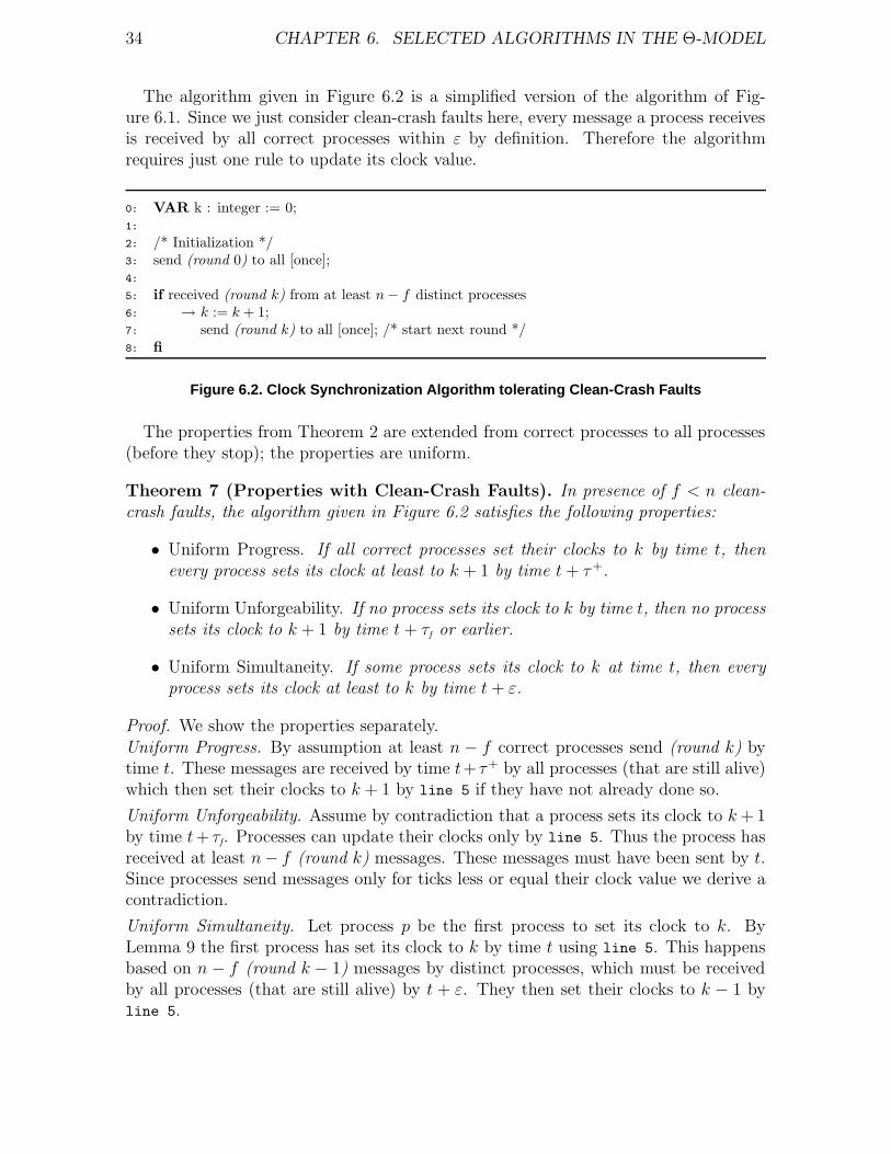
34 CHAPTER 6. SELECTED ALGORITHMS IN THE Θ-MODEL
The algorithm given in Figure 6.2 is a simplified version of the algorithm of Fig-ure 6.1. Since we just consider clean-crash faults here, every message a process receivesis received by all correct processes within ε by definition. Therefore the algorithmrequires just one rule to update its clock value.
0: VAR k : integer := 0;1:
2: /* Initialization */3: send (round 0) to all [once];4:
5: if received (round k) from at least n − f distinct processes6: → k := k + 1;7: send (round k) to all [once]; /* start next round */8: fi
Figure 6.2. Clock Synchronization Algorithm tolerating Clean-Crash Faults
The properties from Theorem 2 are extended from correct processes to all processes(before they stop); the properties are uniform.
Theorem 7 (Properties with Clean-Crash Faults). In presence of f < n clean-crash faults, the algorithm given in Figure 6.2 satisfies the following properties:
• Uniform Progress. If all correct processes set their clocks to k by time t, thenevery process sets its clock at least to k + 1 by time t + τ+.
• Uniform Unforgeability. If no process sets its clock to k by time t, then no processsets its clock to k + 1 by time t + τf or earlier.
• Uniform Simultaneity. If some process sets its clock to k at time t, then everyprocess sets its clock at least to k by time t + ε.
Proof. We show the properties separately.Uniform Progress. By assumption at least n − f correct processes send (round k) bytime t. These messages are received by time t+ τ+ by all processes (that are still alive)which then set their clocks to k + 1 by line 5 if they have not already done so.
Uniform Unforgeability. Assume by contradiction that a process sets its clock to k + 1by time t+ τf. Processes can update their clocks only by line 5. Thus the process hasreceived at least n− f (round k) messages. These messages must have been sent by t.Since processes send messages only for ticks less or equal their clock value we derive acontradiction.
Uniform Simultaneity. Let process p be the first process to set its clock to k. ByLemma 9 the first process has set its clock to k by time t using line 5. This happensbased on n − f (round k − 1) messages by distinct processes, which must be receivedby all processes (that are still alive) by t + ε. They then set their clocks to k − 1 byline 5.
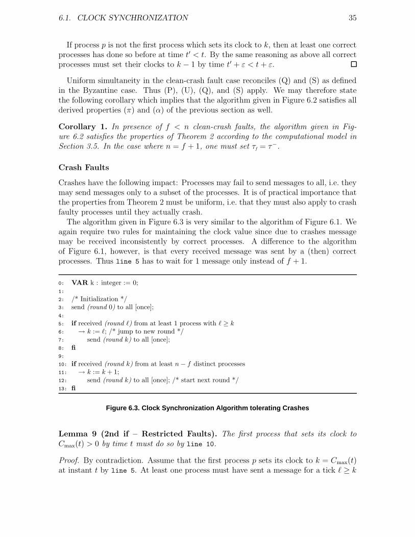
6.1. CLOCK SYNCHRONIZATION 35
If process p is not the first process which sets its clock to k, then at least one correctprocesses has done so before at time t′ < t. By the same reasoning as above all correctprocesses must set their clocks to k − 1 by time t′ + ε < t + ε.
Uniform simultaneity in the clean-crash fault case reconciles (Q) and (S) as definedin the Byzantine case. Thus (P), (U), (Q), and (S) apply. We may therefore statethe following corollary which implies that the algorithm given in Figure 6.2 satisfies allderived properties (π) and (α) of the previous section as well.
Corollary 1. In presence of f < n clean-crash faults, the algorithm given in Fig-ure 6.2 satisfies the properties of Theorem 2 according to the computational model inSection 3.5. In the case where n = f + 1, one must set τf = τ−.
Crash Faults
Crashes have the following impact: Processes may fail to send messages to all, i.e. theymay send messages only to a subset of the processes. It is of practical importance thatthe properties from Theorem 2 must be uniform, i.e. that they must also apply to crashfaulty processes until they actually crash.
The algorithm given in Figure 6.3 is very similar to the algorithm of Figure 6.1. Weagain require two rules for maintaining the clock value since due to crashes messagemay be received inconsistently by correct processes. A difference to the algorithmof Figure 6.1, however, is that every received message was sent by a (then) correctprocesses. Thus line 5 has to wait for 1 message only instead of f + 1.
0: VAR k : integer := 0;1:
2: /* Initialization */3: send (round 0) to all [once];4:
5: if received (round `) from at least 1 process with ` ≥ k6: → k := `; /* jump to new round */7: send (round k) to all [once];8: fi
9:
10: if received (round k) from at least n − f distinct processes11: → k := k + 1;12: send (round k) to all [once]; /* start next round */13: fi
Figure 6.3. Clock Synchronization Algorithm tolerating Crashes
Lemma 9 (2nd if – Restricted Faults). The first process that sets its clock toCmax(t) > 0 by time t must do so by line 10.
Proof. By contradiction. Assume that the first process p sets its clock to k = Cmax(t)at instant t by line 5. At least one process must have sent a message for a tick ` ≥ k
36 CHAPTER 6. SELECTED ALGORITHMS IN THE Θ-MODEL
to enable the rule at p. Since processes only send messages for ticks less or equal thantheir local clock value, at least one must already have a clock value ` ≥ k at instant t.This contradicts p to be the first one that reaches clock value k.
Theorem 8 (Properties with Crashes). In the presence of f < n/2 crash faults,the algorithm given in Figure 6.3 satisfies the following properties:
• Uniform Progress. If all correct processes set their clocks to k by time t, thenevery process sets its clock at least to k + 1 by time t + τ+.
• Uniform Unforgeability. If no process sets its clock to k by time t, then no processsets its clock to k + 1 by time t + τf or earlier.
• Uniform Quasi Simultaneity. If some process sets its clock to k at time t, thenevery process sets its clock at least to k − 1 by time t + ε.
• Uniform Simultaneity. If some process sets its clock to k at time t, then everyprocess sets its clock at least to k by time t + τ+ + ε.
Proof. We show the properties separately.Uniform Progress. By assumption at least n − f correct processes send (round k) bytime t. These messages are received by time t+ τ+ by all processes (that are still alive)which then set their clocks to k + 1 by line 10 if they have not already done so.
Uniform Unforgeability. Assume by contradiction that a process p sets its clock to k+1by time t + τf. Processes may set their clock by (1) line 10 or (2) line 5.
Assume (1). Process p does so based on n − f ≥ f + 1 (round k) messages bydistinct processes. By Lemma 1 at least one of these messages was sent by time t,which provides the required contradiction since processes send messages only for ticksless or equal their clock value.
Assume (2). Process p does so based on one (round k + 1) message, i.e. at least oneprocess has already clock value k + 1 by time t + τf. The first process which has set itsclock to k + 1 must have done so by line 10 by Lemma 9. By applying (1) we againderive a contradiction.
Uniform Quasi Simultaneity. Let process p be the first process to set its clock to k. ByLemma 9 the first process has set its clock to k by time t using line 10. This happensbased on n − f (round k − 1) messages by distinct processes. At least one of thesemust be sent by a correct process whose messages are received by all processes (thatare still alive) by t + ε. They then set their clocks to k − 1 by line 5.
If process p is not the first process which sets its clock to k, then at least one correctprocesses has done so before at time t′ < t. By the same reasoning as above all correctprocesses must set their clocks to k − 1 by time t′ + ε < t + ε.
Uniform Simultaneity. According to uniform quasi simultaneity all processes set theirclock to k − 1 by t + ε. By uniform progress all processes set their clock to k bytime t + τ+ + ε.
As in the case of clean-crash faults the following lemma ascertains the derived prop-erties (π) and (α) from Section 6.1.2 in the case of crash faulty processes.
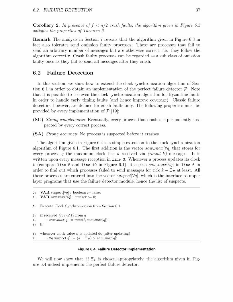
6.2. FAILURE DETECTION 37
Corollary 2. In presence of f < n/2 crash faults, the algorithm given in Figure 6.3satisfies the properties of Theorem 2.
Remark The analysis in Section 7 reveals that the algorithm given in Figure 6.3 infact also tolerates send omission faulty processes. These are processes that fail tosend an arbitrary number of messages but are otherwise correct, i.e. they follow thealgorithm correctly. Crash faulty processes can be regarded as a sub class of omissionfaulty ones as they fail to send all messages after they crash.
6.2 Failure Detection
In this section, we show how to extend the clock synchronization algorithm of Sec-tion 6.1 in order to obtain an implementation of the perfect failure detector P. Notethat it is possible to use even the clock synchronization algorithm for Byzantine faultsin order to handle early timing faults (and hence improve coverage). Classic failuredetectors, however, are defined for crash faults only. The following properties must beprovided by every implementation of P [19]:
(SC) Strong completeness: Eventually, every process that crashes is permanently sus-pected by every correct process.
(SA) Strong accuracy: No process is suspected before it crashes.
The algorithm given in Figure 6.4 is a simple extension to the clock synchronizationalgorithm of Figure 6.1. The first addition is the vector saw max[∀q] that stores forevery process q the maximum clock tick k received via (round k) messages. It iswritten upon every message reception in line 3. Whenever a process updates its clockk (compare line 5 and line 10 in Figure 6.1), it checks saw max[∀q] in line 6 inorder to find out which processes failed to send messages for tick k − ΞP at least. Allthose processes are entered into the vector suspect[∀q], which is the interface to upperlayer programs that use the failure detector module, hence the list of suspects.
0: VAR suspect[∀q] : boolean := false;1: VAR saw max[∀q] : integer := 0;
2: Execute Clock Synchronization from Section 6.1
3: if received (round `) from q4: → saw max[q] := max(`, saw max[q]);5: fi
6: whenever clock value k is updated do (after updating)7: → ∀q suspect[q] := (k − ΞP) > saw max[q];
Figure 6.4. Failure Detector Implementation
We will now show that, if ΞP is chosen appropriately, the algorithm given in Fig-ure 6.4 indeed implements the perfect failure detector.
38 CHAPTER 6. SELECTED ALGORITHMS IN THE Θ-MODEL
Theorem 9. Let ΞP ≥ mind3Ω+1e, d2Ω+2e. In a system with n ≥ 3f+1 processes,the algorithm given in Figure 6.4 implements the perfect failure detector.
Proof. We have to show that strong completeness (SC) and strong accuracy (SA) aresatisfied.
For showing (SC), it is sufficient to notice that a process that crashes after it updatesits clock to ` will be suspected by every correct process p when p reaches clock valuek ≥ ` + ΞP . Since progress of clock values is guaranteed by Lemma 5 every correctprocess will reach clock value k within bounded time (the exact time bound is derivedbelow in Theorem 10).
To prove (SA), we have to show that ΞP is chosen sufficiently large such that everycorrect process which reaches a clock value k at time t has already received messagesfor ticks at least k − ΞP by every correct process. In the worst case setting, a correctprocess p sets its clock to k at instant σk−1
p = σk−1first; hence k = Cmax(σ
k−1p ). From
Lemma 3, it follows that Cmax(σk−1p − τ+) ≥ k − dΩe. Assuming a precision Dmax, a
bound for the smallest possible clock value of a correct process reads Cmin(σk−1p −τ+) ≥
Cmax(σk−1p − τ+)−Dmax = k − dΩe −Dmax. Consequently, every correct process must
have sent a message for tick Cmin(σk−1p − τ+) by time σk−1
p − τ+, which arrives at pby time σk−1
p . Thus, choosing ΞP ≥ dΩe + Dmax is sufficient to ensure that p does notincorrectly suspect any correct process.
Since dxe + dye ≥ dx + ye and d−xe = −bxc, it follows from setting x = z + w andy = −w that dz + we ≥ dze + bwc. By setting z = Ω and bwc = Dmax we employdz+we to choose ΞP . Depending on Ω, precision Ds or Dq is smaller and can be used tocalculate ΞP (by replacing Dmax). Hence, using Ds = b2Ω+1c, we get ΞP ≥ d3Ω+1e.Performing the same calculation for Dq = bΩ + 2c, we get ΞP ≥ d2Ω + 2e.
To find the worst case detection time of our FD algorithm, we have to determine howlong it may take from the time a process p crashes with clock value k until all correctprocesses reach a clock value of k + ΞP and hence suspect p. In the worst case setting,process p has the maximum clock value and crashes immediately after reaching it. Allother processes must first catch up to the maximum value, and then make progress forΞP ticks until correctly suspecting p.
Theorem 10 (Detection Time). The algorithm of Figure 6.4 with the value ΞP
chosen according to Theorem 9 implements the perfect failure detector. Its detectiontime is bounded by (ΞP + 2)τ+ − τ−.
Proof. Assume the worst case: A process p is crashing at time tc where k = Cp(tc) =Cmax(tc). By (S) in Theorem 2 every correct process must reach clock value k bytime t′ = tc + τ+ + ε. When a correct process reaches clock value k + ΞP it willsuspect p. By Lemma 5 every correct process must reach that clock value by timet = t′ + ΞPτ+ = tc + τ+ + ε + ΞP τ+ = tc + (ΞP + 2) τ+ − τ−.
The detection time in Theorem 10 is given in the context of the computational modelof Section 3.3. In order to give the detection time in the system model of Section 3.2,
6.3. SYNCHRONY OF THE Θ-MODEL 39
one has to transfer the times tc and tc + (ΞP + 2) Ω − 1 (see Equation 3.1) into real-time. The detection latency is hence given by ∆t = β−1(tc + (ΞP + 2) Ω− 1)− β−1(tc).When immersing the failure detector algorithm into a real system one has to considerτ+ (compare Section 5.1) in order to derive the worst case detection time. Followingthe fast failure detector approach [51, 1] these detection times are much smaller thanapplication level message delays. Using this approach it is hence possible to devisevery efficient agreement algorithms.
Note that our failure detector implementation relies upon the totally time free clocksynchronization algorithm from Section 6.1. The latter algorithm has no a priori knowl-edge of Θ such that violations of Θ do not do any harm to the correctness of thealgorithm. Just the calculated bounds on (π) and (α) are violated. Consider the vari-ant of the Θ-Model where Θ just holds from some unknown global stabilization time(GST) on [37, 19, 107]. Our clock synchronization algorithm will return to its predictedbehavior within a short period of time.
Theorem 11 (Eventually Perfect Failure Detector). When executed in a systemwhere Θ (see system model, Section 3.2) holds from some unknown time GST on, thealgorithm of Figure 6.4 with the value ΞP chosen according to Theorem 9 implementsthe eventually perfect failure detector P.
Proof. Let k − 1 = Cmax(GST ). After time t = σkfirst + ε all correct processes have set
their clocks based on messages by correct processes which were sent after GST. Thus(P), (U), (Q), and (S) apply for all rounds greater than k with values τ+ and τ− (aswell as ε), satisfying the Θ assumption. Hence (π) and (α) are as predicted for theserounds. Thus Theorem 9 and Theorem 10 apply from time t on.
Remark Note that we devised an alternative implementation [55] of P that worksin networks with n > f in the presence of up to f crash faults. It can also be usedas a local FD [54] in sparse networks where just the neighbors have to be observed. Avariant of this algorithm can be applied in order to get the leader oracle—the weakestFD which allows to solve asynchronous consensus [18]—both in sparsely and fullyconnected networks.
6.3 Synchrony of the Θ-Model
When taking a closer look at the implementation of P in Section 6.2 it turns outthat is has stronger semantics than just (SC) and (SA): When a process detects a crashfrom process p it can also be sure that no more messages from p are in transit. Thisreveals that the Θ-Model allows a correct process p to determine an instant t when itis guaranteed that no more earlier messages from a given process will arrive at p aftertime t. A problem that can be reduced to the decision of whether a message fromsome process is still in transit is the strongly dependent decision problem [21]. In thefollowing section we will give a solution for this problem.
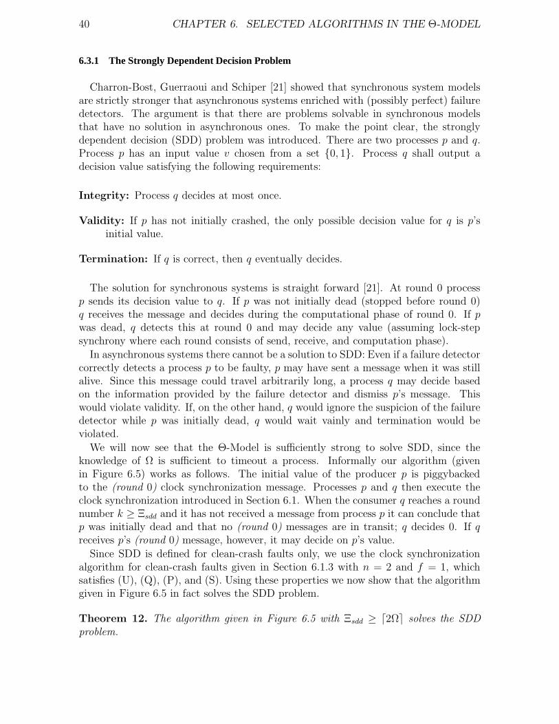
40 CHAPTER 6. SELECTED ALGORITHMS IN THE Θ-MODEL
6.3.1 The Strongly Dependent Decision Problem
Charron-Bost, Guerraoui and Schiper [21] showed that synchronous system modelsare strictly stronger that asynchronous systems enriched with (possibly perfect) failuredetectors. The argument is that there are problems solvable in synchronous modelsthat have no solution in asynchronous ones. To make the point clear, the stronglydependent decision (SDD) problem was introduced. There are two processes p and q.Process p has an input value v chosen from a set 0, 1. Process q shall output adecision value satisfying the following requirements:
Integrity: Process q decides at most once.
Validity: If p has not initially crashed, the only possible decision value for q is p’sinitial value.
Termination: If q is correct, then q eventually decides.
The solution for synchronous systems is straight forward [21]. At round 0 processp sends its decision value to q. If p was not initially dead (stopped before round 0)q receives the message and decides during the computational phase of round 0. If pwas dead, q detects this at round 0 and may decide any value (assuming lock-stepsynchrony where each round consists of send, receive, and computation phase).
In asynchronous systems there cannot be a solution to SDD: Even if a failure detectorcorrectly detects a process p to be faulty, p may have sent a message when it was stillalive. Since this message could travel arbitrarily long, a process q may decide basedon the information provided by the failure detector and dismiss p’s message. Thiswould violate validity. If, on the other hand, q would ignore the suspicion of the failuredetector while p was initially dead, q would wait vainly and termination would beviolated.
We will now see that the Θ-Model is sufficiently strong to solve SDD, since theknowledge of Ω is sufficient to timeout a process. Informally our algorithm (givenin Figure 6.5) works as follows. The initial value of the producer p is piggybackedto the (round 0) clock synchronization message. Processes p and q then execute theclock synchronization introduced in Section 6.1. When the consumer q reaches a roundnumber k ≥ Ξsdd and it has not received a message from process p it can conclude thatp was initially dead and that no (round 0) messages are in transit; q decides 0. If qreceives p’s (round 0) message, however, it may decide on p’s value.
Since SDD is defined for clean-crash faults only, we use the clock synchronizationalgorithm for clean-crash faults given in Section 6.1.3 with n = 2 and f = 1, whichsatisfies (U), (Q), (P), and (S). Using these properties we now show that the algorithmgiven in Figure 6.5 in fact solves the SDD problem.
Theorem 12. The algorithm given in Figure 6.5 with Ξsdd ≥ d2Ωe solves the SDDproblem.
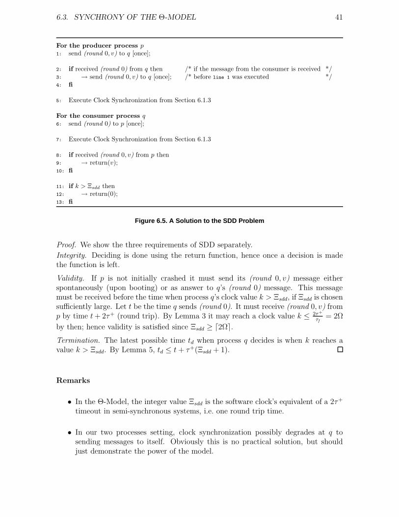
6.3. SYNCHRONY OF THE Θ-MODEL 41
For the producer process p1: send (round 0, v) to q [once];
2: if received (round 0) from q then /* if the message from the consumer is received */3: → send (round 0, v) to q [once]; /* before line 1 was executed */4: fi
5: Execute Clock Synchronization from Section 6.1.3
For the consumer process q6: send (round 0) to p [once];
7: Execute Clock Synchronization from Section 6.1.3
8: if received (round 0, v) from p then9: → return(v);10: fi
11: if k > Ξsdd then12: → return(0);13: fi
Figure 6.5. A Solution to the SDD Problem
Proof. We show the three requirements of SDD separately.
Integrity. Deciding is done using the return function, hence once a decision is madethe function is left.
Validity. If p is not initially crashed it must send its (round 0, v) message eitherspontaneously (upon booting) or as answer to q’s (round 0) message. This messagemust be received before the time when process q’s clock value k > Ξsdd, if Ξsdd is chosensufficiently large. Let t be the time q sends (round 0). It must receive (round 0, v) fromp by time t + 2τ+ (round trip). By Lemma 3 it may reach a clock value k ≤ 2τ+
τf= 2Ω
by then; hence validity is satisfied since Ξsdd ≥ d2Ωe.
Termination. The latest possible time td when process q decides is when k reaches avalue k > Ξsdd. By Lemma 5, td ≤ t + τ+(Ξsdd + 1).
Remarks
• In the Θ-Model, the integer value Ξsdd is the software clock’s equivalent of a 2τ+
timeout in semi-synchronous systems, i.e. one round trip time.
• In our two processes setting, clock synchronization possibly degrades at q tosending messages to itself. Obviously this is no practical solution, but shouldjust demonstrate the power of the model.
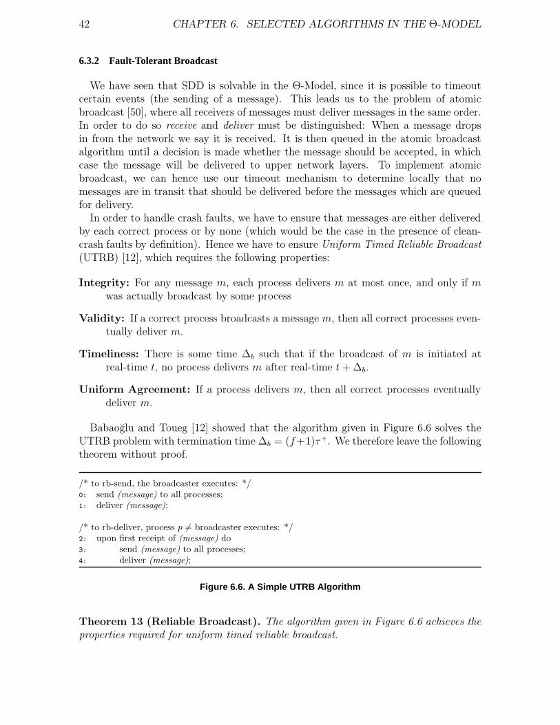
42 CHAPTER 6. SELECTED ALGORITHMS IN THE Θ-MODEL
6.3.2 Fault-Tolerant Broadcast
We have seen that SDD is solvable in the Θ-Model, since it is possible to timeoutcertain events (the sending of a message). This leads us to the problem of atomicbroadcast [50], where all receivers of messages must deliver messages in the same order.In order to do so receive and deliver must be distinguished: When a message dropsin from the network we say it is received. It is then queued in the atomic broadcastalgorithm until a decision is made whether the message should be accepted, in whichcase the message will be delivered to upper network layers. To implement atomicbroadcast, we can hence use our timeout mechanism to determine locally that nomessages are in transit that should be delivered before the messages which are queuedfor delivery.
In order to handle crash faults, we have to ensure that messages are either deliveredby each correct process or by none (which would be the case in the presence of clean-crash faults by definition). Hence we have to ensure Uniform Timed Reliable Broadcast(UTRB) [12], which requires the following properties:
Integrity: For any message m, each process delivers m at most once, and only if mwas actually broadcast by some process
Validity: If a correct process broadcasts a message m, then all correct processes even-tually deliver m.
Timeliness: There is some time ∆b such that if the broadcast of m is initiated atreal-time t, no process delivers m after real-time t + ∆b.
Uniform Agreement: If a process delivers m, then all correct processes eventuallydeliver m.
Babaoglu and Toueg [12] showed that the algorithm given in Figure 6.6 solves theUTRB problem with termination time ∆b = (f+1)τ+. We therefore leave the followingtheorem without proof.
/* to rb-send, the broadcaster executes: */0: send (message) to all processes;1: deliver (message);
/* to rb-deliver, process p 6= broadcaster executes: */2: upon first receipt of (message) do3: send (message) to all processes;4: deliver (message);
Figure 6.6. A Simple UTRB Algorithm
Theorem 13 (Reliable Broadcast). The algorithm given in Figure 6.6 achieves theproperties required for uniform timed reliable broadcast.

6.3. SYNCHRONY OF THE Θ-MODEL 43
In addition to the properties of reliable broadcast, atomic broadcast requires thatall processes deliver the messages in total order.
Total Order: If processes p and q both deliver messages m and m′, then p delivers mbefore m′ if and only if q delivers m before m′.
We will see that this can be achieved in the Θ-Model. In fact, the algorithm given inFigure 6.7 solves FIFO-Atomic-Broadcast (FIFO refers to the property that messagessent by process p are received in the same order as p has sent them). Note that thealgorithm integrates the reliable broadcast algorithm from Figure 6.6.
/* Broadcaster s executes: */0: send (message, s, Cs, i) to all processes /* Cs is the local time stamp */1: queue (message, s, Cs, i) for delivery /* i is the sequence number */
/* Process q 6= broadcaster executes: */2: upon first receipt of (message, s, Cs, i)3: → send (message, s, Cs, i) to all processes4: queue (message, s, Cs, i) for delivery
/* Any process p executes: */5: whenever clock k is updated do (after updating)6: → delivera all queued messages with time stamp Cs ≤ Cp − Ξabc
7: Execute Clock Synchronization from Section 6.1.3
aordered by (1) increasing timestamps, (2) in-creasing process identifiers, and (3) increasing in-dexes i
Figure 6.7. A Simple Atomic Broadcast Algorithm in the Θ-Model
For the algorithm in Figure 6.7, we assume that all processes have synchronizedclocks according to Section 6.1. Every process s that wishes to broadcast a messageat time t, timestamps this message with its local clock value Cs(tsend) and assigns anindex i to it, i.e. a local sequence number that makes every message unique. This isrequired since processes may broadcast multiple message during one round, i.e. thetime stamp is not sufficient for total ordering. Then it initiates a reliable broadcast(line 0-1). Each correct process p which receives a messages forwards the messagewith its original time stamp, according to the reliable broadcast algorithm (line 2-4).Instead of delivering immediately, p waits for delivery until it reaches a local clockvalue Cp = Cs(tsend) + Ξabc (line 5-6). If two processes initiate a broadcast with thesame time stamp the process identifier has to be used in order to establish a consistentdelivery order. Since all processes deliver the same message during the same localround, message are totally ordered.
Theorem 14. The algorithm given in Figure 6.7 with Ξabc ≥ bΩ(f + 1)c + Dq solvesthe atomic broadcast problem.
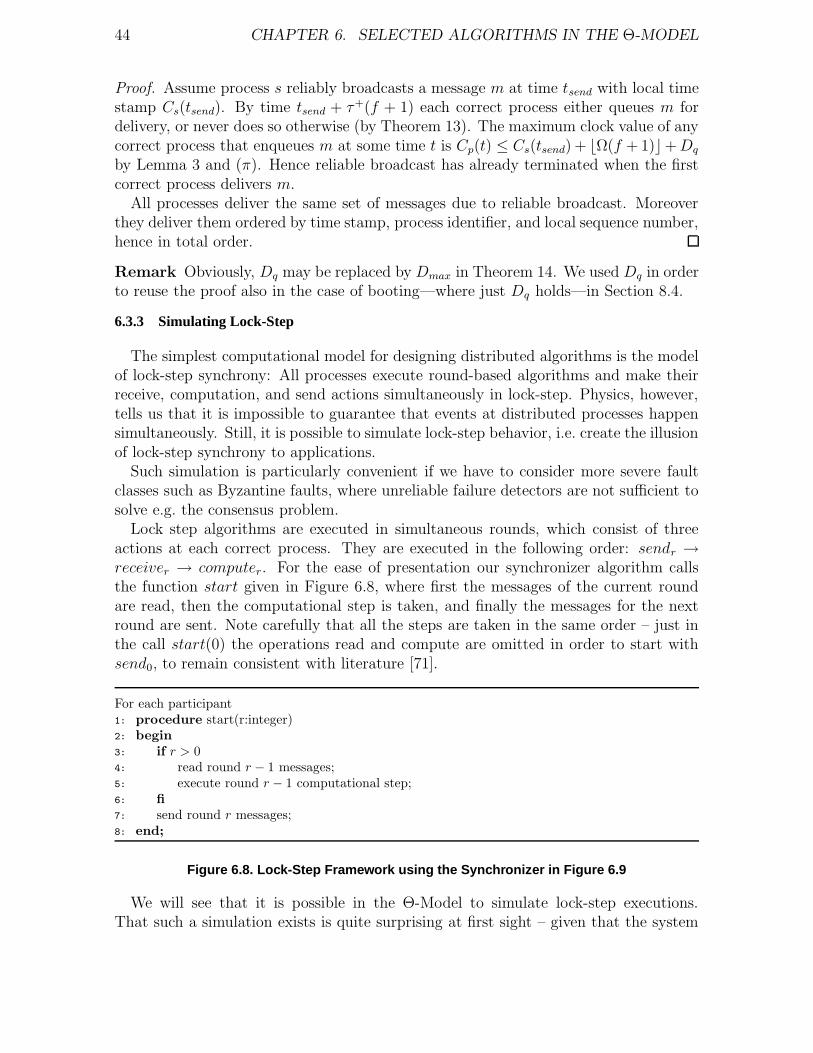
44 CHAPTER 6. SELECTED ALGORITHMS IN THE Θ-MODEL
Proof. Assume process s reliably broadcasts a message m at time tsend with local timestamp Cs(tsend). By time tsend + τ+(f + 1) each correct process either queues m fordelivery, or never does so otherwise (by Theorem 13). The maximum clock value of anycorrect process that enqueues m at some time t is Cp(t) ≤ Cs(tsend) + bΩ(f + 1)c+ Dq
by Lemma 3 and (π). Hence reliable broadcast has already terminated when the firstcorrect process delivers m.
All processes deliver the same set of messages due to reliable broadcast. Moreoverthey deliver them ordered by time stamp, process identifier, and local sequence number,hence in total order.
Remark Obviously, Dq may be replaced by Dmax in Theorem 14. We used Dq in orderto reuse the proof also in the case of booting—where just Dq holds—in Section 8.4.
6.3.3 Simulating Lock-Step
The simplest computational model for designing distributed algorithms is the modelof lock-step synchrony: All processes execute round-based algorithms and make theirreceive, computation, and send actions simultaneously in lock-step. Physics, however,tells us that it is impossible to guarantee that events at distributed processes happensimultaneously. Still, it is possible to simulate lock-step behavior, i.e. create the illusionof lock-step synchrony to applications.
Such simulation is particularly convenient if we have to consider more severe faultclasses such as Byzantine faults, where unreliable failure detectors are not sufficient tosolve e.g. the consensus problem.
Lock step algorithms are executed in simultaneous rounds, which consist of threeactions at each correct process. They are executed in the following order: sendr →receiver → computer. For the ease of presentation our synchronizer algorithm callsthe function start given in Figure 6.8, where first the messages of the current roundare read, then the computational step is taken, and finally the messages for the nextround are sent. Note carefully that all the steps are taken in the same order – just inthe call start(0) the operations read and compute are omitted in order to start withsend0, to remain consistent with literature [71].
For each participant1: procedure start(r:integer)2: begin
3: if r > 04: read round r − 1 messages;5: execute round r − 1 computational step;6: fi
7: send round r messages;8: end;
Figure 6.8. Lock-Step Framework using the Synchronizer in Figure 6.9
We will see that it is possible in the Θ-Model to simulate lock-step executions.That such a simulation exists is quite surprising at first sight – given that the system
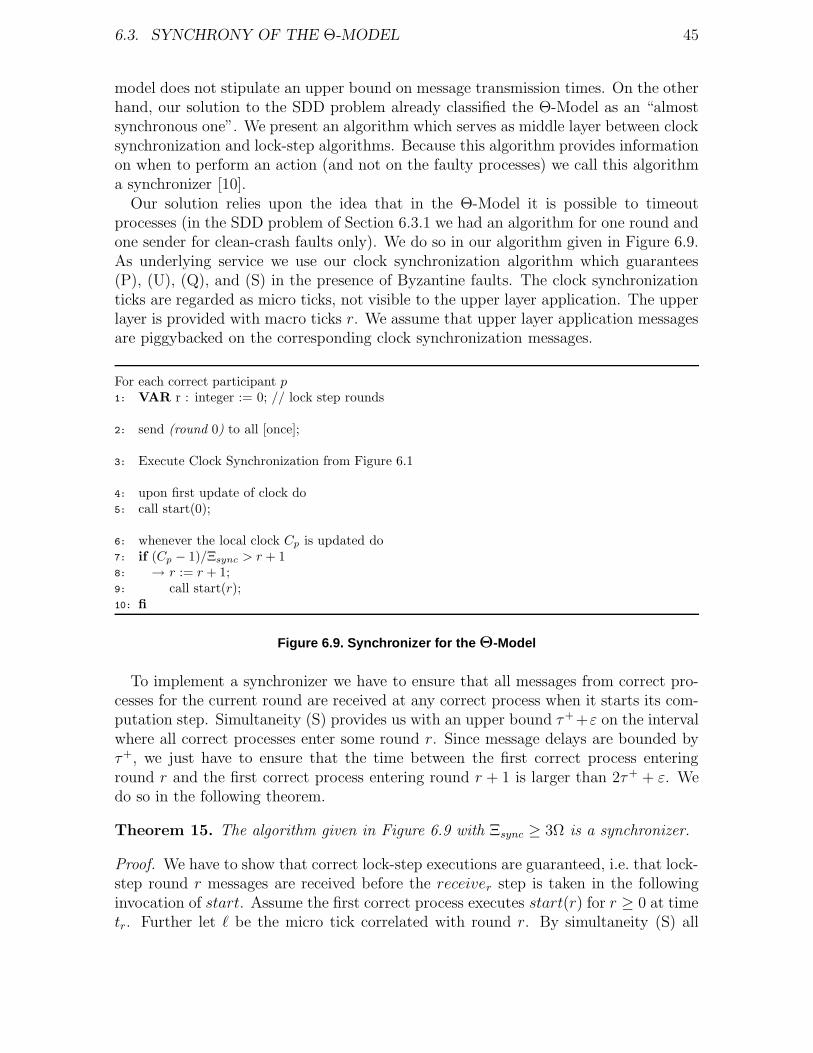
6.3. SYNCHRONY OF THE Θ-MODEL 45
model does not stipulate an upper bound on message transmission times. On the otherhand, our solution to the SDD problem already classified the Θ-Model as an “almostsynchronous one”. We present an algorithm which serves as middle layer between clocksynchronization and lock-step algorithms. Because this algorithm provides informationon when to perform an action (and not on the faulty processes) we call this algorithma synchronizer [10].
Our solution relies upon the idea that in the Θ-Model it is possible to timeoutprocesses (in the SDD problem of Section 6.3.1 we had an algorithm for one round andone sender for clean-crash faults only). We do so in our algorithm given in Figure 6.9.As underlying service we use our clock synchronization algorithm which guarantees(P), (U), (Q), and (S) in the presence of Byzantine faults. The clock synchronizationticks are regarded as micro ticks, not visible to the upper layer application. The upperlayer is provided with macro ticks r. We assume that upper layer application messagesare piggybacked on the corresponding clock synchronization messages.
For each correct participant p1: VAR r : integer := 0; // lock step rounds
2: send (round 0) to all [once];
3: Execute Clock Synchronization from Figure 6.1
4: upon first update of clock do5: call start(0);
6: whenever the local clock Cp is updated do7: if (Cp − 1)/Ξsync > r + 18: → r := r + 1;9: call start(r);10: fi
Figure 6.9. Synchronizer for the Θ-Model
To implement a synchronizer we have to ensure that all messages from correct pro-cesses for the current round are received at any correct process when it starts its com-putation step. Simultaneity (S) provides us with an upper bound τ+ +ε on the intervalwhere all correct processes enter some round r. Since message delays are bounded byτ+, we just have to ensure that the time between the first correct process enteringround r and the first correct process entering round r + 1 is larger than 2τ+ + ε. Wedo so in the following theorem.
Theorem 15. The algorithm given in Figure 6.9 with Ξsync ≥ 3Ω is a synchronizer.
Proof. We have to show that correct lock-step executions are guaranteed, i.e. that lock-step round r messages are received before the receiver step is taken in the followinginvocation of start. Assume the first correct process executes start(r) for r ≥ 0 at timetr. Further let ` be the micro tick correlated with round r. By simultaneity (S) all
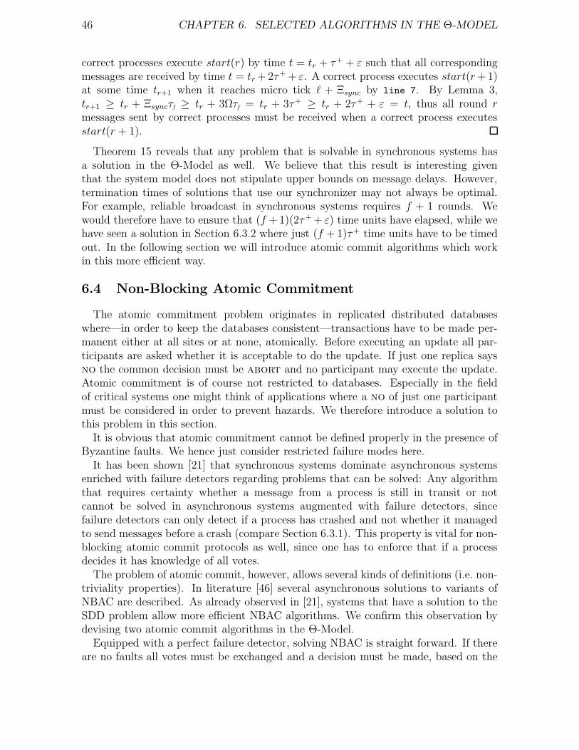
46 CHAPTER 6. SELECTED ALGORITHMS IN THE Θ-MODEL
correct processes execute start(r) by time t = tr + τ+ + ε such that all correspondingmessages are received by time t = tr +2τ+ + ε. A correct process executes start(r +1)at some time tr+1 when it reaches micro tick ` + Ξsync by line 7. By Lemma 3,tr+1 ≥ tr + Ξsyncτf ≥ tr + 3Ωτf = tr + 3τ+ ≥ tr + 2τ+ + ε = t, thus all round rmessages sent by correct processes must be received when a correct process executesstart(r + 1).
Theorem 15 reveals that any problem that is solvable in synchronous systems hasa solution in the Θ-Model as well. We believe that this result is interesting giventhat the system model does not stipulate upper bounds on message delays. However,termination times of solutions that use our synchronizer may not always be optimal.For example, reliable broadcast in synchronous systems requires f + 1 rounds. Wewould therefore have to ensure that (f +1)(2τ+ + ε) time units have elapsed, while wehave seen a solution in Section 6.3.2 where just (f + 1)τ+ time units have to be timedout. In the following section we will introduce atomic commit algorithms which workin this more efficient way.
6.4 Non-Blocking Atomic Commitment
The atomic commitment problem originates in replicated distributed databaseswhere—in order to keep the databases consistent—transactions have to be made per-manent either at all sites or at none, atomically. Before executing an update all par-ticipants are asked whether it is acceptable to do the update. If just one replica saysno the common decision must be abort and no participant may execute the update.Atomic commitment is of course not restricted to databases. Especially in the fieldof critical systems one might think of applications where a no of just one participantmust be considered in order to prevent hazards. We therefore introduce a solution tothis problem in this section.
It is obvious that atomic commitment cannot be defined properly in the presence ofByzantine faults. We hence just consider restricted failure modes here.
It has been shown [21] that synchronous systems dominate asynchronous systemsenriched with failure detectors regarding problems that can be solved: Any algorithmthat requires certainty whether a message from a process is still in transit or notcannot be solved in asynchronous systems augmented with failure detectors, sincefailure detectors can only detect if a process has crashed and not whether it managedto send messages before a crash (compare Section 6.3.1). This property is vital for non-blocking atomic commit protocols as well, since one has to enforce that if a processdecides it has knowledge of all votes.
The problem of atomic commit, however, allows several kinds of definitions (i.e. non-triviality properties). In literature [46] several asynchronous solutions to variants ofNBAC are described. As already observed in [21], systems that have a solution to theSDD problem allow more efficient NBAC algorithms. We confirm this observation bydevising two atomic commit algorithms in the Θ-Model.
Equipped with a perfect failure detector, solving NBAC is straight forward. If thereare no faults all votes must be exchanged and a decision must be made, based on the
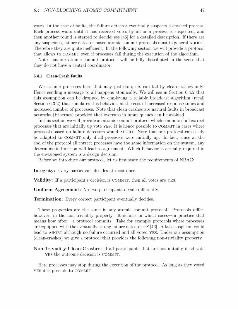
6.4. NON-BLOCKING ATOMIC COMMITMENT 47
votes. In the case of faults, the failure detector eventually suspects a crashed process.Each process waits until it has received votes by all or a process is suspected, andthen another round is started to decide; see [46] for a detailed description. If there areany suspicions, failure detector based atomic commit protocols must in general abort.Therefore they are quite inefficient. In the following section we will provide a protocolthat allows to commit even if processes fail during the execution of the algorithm.
Note that our atomic commit protocols will be fully distributed in the sense thatthey do not have a central coordinator.
6.4.1 Clean-Crash Faults
We assume processes here that may just stop, i.e. can fail by clean-crashes only:Hence sending a message to all happens atomically. We will see in Section 6.4.2 thatthis assumption can be dropped by employing a reliable broadcast algorithm (recallSection 6.3.2) that simulates this behavior, at the cost of increased response times andincreased number of processes. Note that clean crashes are natural faults in broadcastnetworks (Ethernet) provided that overruns in input queues can be avoided.
In this section we will provide an atomic commit protocol which commits if all correctprocesses that are initially up vote yes. It is hence possible to commit in cases whereprotocols based on failure detectors would abort. Note that our protocol can easilybe adapted to commit only if all processes were initially up. In fact, since at theend of the protocol all correct processes have the same information on the system, anydeterministic function will lead to agreement. Which behavior is actually required inthe envisioned system is a design decision.
Before we introduce our protocol, let us first state the requirements of NBAC:
Integrity: Every participant decides at most once.
Validity: If a participant’s decision is commit, then all votes are yes.
Uniform Agreement: No two participants decide differently.
Termination: Every correct participant eventually decides.
These properties are the same in any atomic commit protocol. Protocols differ,however, in the non-triviality property. It defines in which cases—in practice thatmeans how often—a protocol commits. Take for example protocols where processesare equipped with the eventually strong failure detector S [46]. A false suspicion couldlead to abort although no failure occurred and all voted yes. Under our assumption(clean-crashes) we give a protocol that provides the following non-triviality property.
Non-Triviality-Clean-Crashes: If all participants that are not initially dead voteyes the outcome decision is commit.
Here processes may stop during the execution of the protocol. As long as they votedyes it is possible to commit.
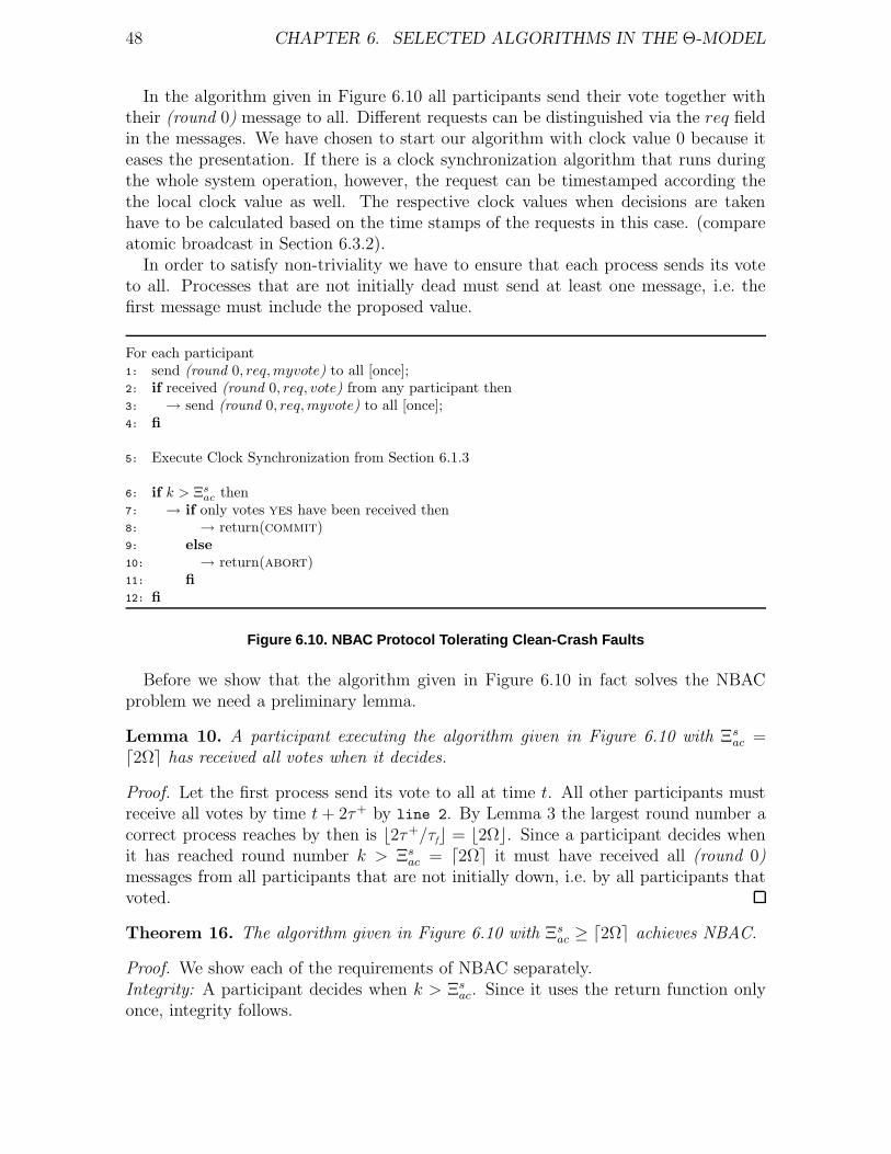
48 CHAPTER 6. SELECTED ALGORITHMS IN THE Θ-MODEL
In the algorithm given in Figure 6.10 all participants send their vote together withtheir (round 0) message to all. Different requests can be distinguished via the req fieldin the messages. We have chosen to start our algorithm with clock value 0 because iteases the presentation. If there is a clock synchronization algorithm that runs duringthe whole system operation, however, the request can be timestamped according thethe local clock value as well. The respective clock values when decisions are takenhave to be calculated based on the time stamps of the requests in this case. (compareatomic broadcast in Section 6.3.2).
In order to satisfy non-triviality we have to ensure that each process sends its voteto all. Processes that are not initially dead must send at least one message, i.e. thefirst message must include the proposed value.
For each participant1: send (round 0, req, myvote) to all [once];2: if received (round 0, req, vote) from any participant then3: → send (round 0, req, myvote) to all [once];4: fi
5: Execute Clock Synchronization from Section 6.1.3
6: if k > Ξsac then
7: → if only votes yes have been received then8: → return(commit)9: else
10: → return(abort)11: fi
12: fi
Figure 6.10. NBAC Protocol Tolerating Clean-Crash Faults
Before we show that the algorithm given in Figure 6.10 in fact solves the NBACproblem we need a preliminary lemma.
Lemma 10. A participant executing the algorithm given in Figure 6.10 with Ξsac =
d2Ωe has received all votes when it decides.
Proof. Let the first process send its vote to all at time t. All other participants mustreceive all votes by time t + 2τ+ by line 2. By Lemma 3 the largest round number acorrect process reaches by then is b2τ+/τfc = b2Ωc. Since a participant decides whenit has reached round number k > Ξs
ac = d2Ωe it must have received all (round 0)messages from all participants that are not initially down, i.e. by all participants thatvoted.
Theorem 16. The algorithm given in Figure 6.10 with Ξsac ≥ d2Ωe achieves NBAC.
Proof. We show each of the requirements of NBAC separately.Integrity: A participant decides when k > Ξs
ac. Since it uses the return function onlyonce, integrity follows.
6.4. NON-BLOCKING ATOMIC COMMITMENT 49
Validity: Lemma 10 states that if a participant decides, it has received all votes. Byline 7 it only decides commit if all votes where yes.
Uniform Agreement: If a process decides, it has received all votes. Any two participantshence decide on the same set of messages and must therefore decide the same value.
Termination: Every correct process decides when it reaches round k > Ξsac. Let t be
the time the first process sends its (round 0) message. By line 2 all processes send(round 0) by time t + τ+, which is the assumption of (P). Therefore every correctprocess reaches round k by time t + τ+ + τ+Ξs
ac ≥ t + τ+(2Ω + 1) (see Lemma 5).
Non-Triviality: If all votes are yes, by line 7 every outcome must be commit.
Remark From simultaneity (S) follows that all correct processes reach round k > Ξsac
within τ+ + ε, such that they commit within a short period of time. This is importantin the context of real-time systems as well.
6.4.2 Crashes
It is well known that for systems where processes may crash during the executionof a step, reliable broadcast is required in order to keep the views of the remainingprocesses consistent (compare Section 6.3.2). To solve NBAC in this case, we employan adaptation of the protocols from [83] which are based upon a semi-synchronoussystem model, where upper time bounds on transmission and computation steps areknown, and the processes are equipped with local hardware clocks with known drift.We will see that our software clocks can be employed in the same manner, withoutknowing the bounds on transmission and computation steps.
Due to the more severe failure mode, it is not possible to satisfy the same non-triviality property as if only clean-crash failures had to be considered. This section’sprotocol achieves the following property:
Non-Triviality-Crashes: If all processes vote yes and no failure occurs, then theoutcome decision is commit.
As in the case of clean-crash failures we start with a preliminary lemma whichguarantees equal sets of messages at all processes when the decision is made.
Lemma 11. All participants executing the algorithm given in Figure 6.11 with Ξcac ≥
dΩ(f + 2)e have delivered the same votes when they decide.
Proof. If there are no faults and all vote yes by reliable broadcast all deliver thesevotes and decide in line 9. If there is one vote no and one process delivers it, byreliable broadcast all deliver it and decide in line 3. We have to show that if one ofthese two cases happen, they happen at every process before line 6 is enabled.
Let the first process enter round ` > Ξcac where it decides using line 6 at time t′. By
Lemma 3 the first process enters round 1 not after time t ≤ t′−Ξcacτf. By (Q) hence all
processes send (round 0) by time t+ε and reliably broadcast their vote. By Theorem 13all the votes are delivered by time t′′ = t+ε+(f +1)τ+ < t+(f +2)τ+ = t+Ξc
acτf ≤ t′.Since t′′ < t′ our lemma is true.
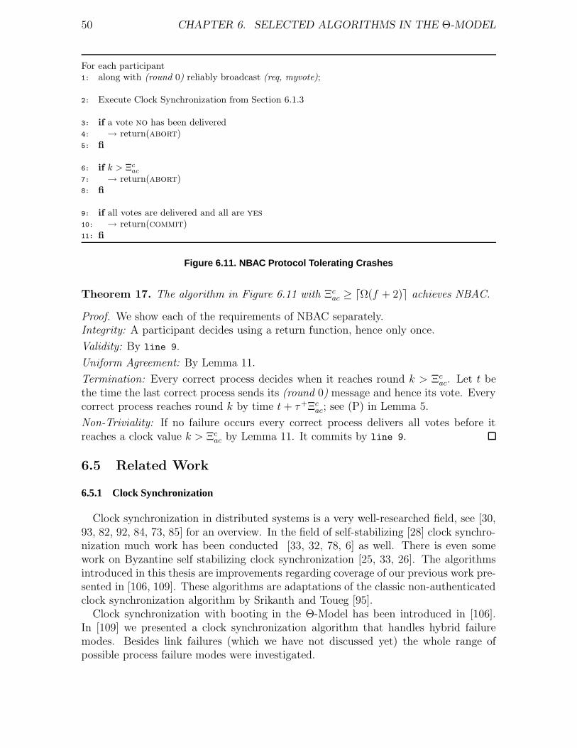
50 CHAPTER 6. SELECTED ALGORITHMS IN THE Θ-MODEL
For each participant1: along with (round 0) reliably broadcast (req, myvote);
2: Execute Clock Synchronization from Section 6.1.3
3: if a vote no has been delivered4: → return(abort)5: fi
6: if k > Ξcac
7: → return(abort)8: fi
9: if all votes are delivered and all are yes
10: → return(commit)11: fi
Figure 6.11. NBAC Protocol Tolerating Crashes
Theorem 17. The algorithm in Figure 6.11 with Ξcac ≥ dΩ(f + 2)e achieves NBAC.
Proof. We show each of the requirements of NBAC separately.Integrity: A participant decides using a return function, hence only once.
Validity: By line 9.
Uniform Agreement: By Lemma 11.
Termination: Every correct process decides when it reaches round k > Ξcac. Let t be
the time the last correct process sends its (round 0) message and hence its vote. Everycorrect process reaches round k by time t + τ+Ξc
ac; see (P) in Lemma 5.
Non-Triviality: If no failure occurs every correct process delivers all votes before itreaches a clock value k > Ξc
ac by Lemma 11. It commits by line 9.
6.5 Related Work
6.5.1 Clock Synchronization
Clock synchronization in distributed systems is a very well-researched field, see [30,93, 82, 92, 84, 73, 85] for an overview. In the field of self-stabilizing [28] clock synchro-nization much work has been conducted [33, 32, 78, 6] as well. There is even somework on Byzantine self stabilizing clock synchronization [25, 33, 26]. The algorithmsintroduced in this thesis are improvements regarding coverage of our previous work pre-sented in [106, 109]. These algorithms are adaptations of the classic non-authenticatedclock synchronization algorithm by Srikanth and Toueg [95].
Clock synchronization with booting in the Θ-Model has been introduced in [106].In [109] we presented a clock synchronization algorithm that handles hybrid failuremodes. Besides link failures (which we have not discussed yet) the whole range ofpossible process failure modes were investigated.
6.5. RELATED WORK 51
6.5.2 Unreliable Failure Detectors
Failure detectors are particularly attractive, since they encapsulate synchrony as-sumptions in a time free manner. Consensus algorithms using FDs are hence com-pletely time free and thus share the coverage maximization property proper to purelyasynchronous algorithms. Nevertheless, the question of coverage arises also when im-plementing a failure detector, which of course requires the underlying system to satisfyat least some synchrony assumptions. In fact, existing implementations of the perfectfailure detector P rest upon knowing the bounds on the end-to-end transmission delaysof messages and hence require a synchronous system.
Since it has been shown in [63] that perpetual FDs cannot be implemented in par-tially synchronous systems with unknown delay bounds [37, 19], perpetual accuracyproperties like strong accuracy (“no processor is suspected before it crashes”) are usu-ally replaced by eventual ones (“there is a time after which correct processors are notsuspected by any correct processor”). Many papers deal with the implementation ofsuch eventual-type FDs [19, 61, 62, 22, 48, 40, 51, 15, 2]. Eventual properties are usuallyin conflict with the timeliness requirements of real-time systems, however. Neverthe-less if an algorithm, designed to work with an eventual FD, uses a perpetual FD thatprovides bounded detection times, real-time properties can be achieved here as well.
In purely asynchronous systems, it is impossible to implement even eventual-typefailure detectors. FDs with very weak specifications [44, 4] have been proposed as analternative here. The heartbeat failure detectors of [4] do not output a list of suspectsbut rather a list of unbounded counters. Like P, they permit to solve the importantproblem of quiescent reliable communication in the presence of crashes, but unlike P,they can easily be implemented in purely asynchronous systems.
In view of the impossibility results of [29] and [63], it was taken for granted untilrecently that implementing perpetual failure detectors requires accurate knowledge ofdelay bounds and hence a synchronous system model. Still, the algorithms presentedin [76, 75] reveal that perpetual FDs can be implemented in a time-free manner insystems with specific properties. For example, there is a time-free implementation ofP in systems where it can be assumed a priori that every correct processor is connectedto a set of f +1 processors via links that are not among their f slowest ones. The algo-rithm cannot verify whether the underlying system actually satisfies this assumption,however, and no design for implementing this property was given.
The failure detector presented in this thesis follows an idea that was originally de-veloped by Le Lann and Schmid [67]. There exists subsequent work on this approachregarding coverage maximization [68] and system booting [108].
6.5.3 Synchronizers
In literature several approaches have been proposed to simulate synchronous sys-tems, see also [9] for an overview on several simulation techniques.. Awerbuch [10]introduced the term synchronizer to describe algorithms that simulate synchronousnetworks in asynchronous ones. The algorithms he presented could be used in net-works with arbitrary topologies, but only in the absence of faults.
52 CHAPTER 6. SELECTED ALGORITHMS IN THE Θ-MODEL
Dwork, Lynch and Stockmeyer [37] devised several simulations for lock-step syn-chrony in the presence of partial synchrony for several types of process failures (includ-ing non-authenticated Byzantine). These simulations reach lock-step behavior eventu-ally. In the global stabilization time model it is reached after the system has stabilized.In the case where the timing bounds are unknown the round durations are increased,and lock-step is reached when the rounds are sufficiently long.
Round-by-round fault detectors where introduced by Gafni [43]. Such fault detectorsprovide some process p—running a round based algorithm—with information aboutother processes which might have crashed. If all processes from whom no message forthe current round has dropped in are suspected, the next round is entered.
6.5.4 Non-Blocking Atomic Commit
Consensus [9, 71] and non-blocking atomic commitment [83, 46, 38, 27, 12] are verysimilar agreement problems. Their relation is investigated in [47, 20] and Guerraouishows in [47] that these problems are not comparable in asynchronous systems.
The uniform timed reliable broadcast algorithm we employed can be found in [12],where several other topics related to atomic commitment are discussed as well
Guerraoui and Schiper [46] presented decentralized non-blocking commit protocols.In contrast to the classical two phase commit and three phase commit these protocolsdo not have a central coordinator. The algorithm in [46] rely upon the eventuallystrong failure detector S. In [83] several non-blocking atomic commitment algorithmsare presented and investigated for several system models—from synchronous to asyn-chronous with failure detectors. Timed atomic commit was introduced in [27]. Thealgorithm that was presented there uses local hardware clocks in order to detect thattiming constraints are violated.
Lower bounds regarding message complexity as well as timing complexity can befound in [38].
Chapter 7
Booting Clock Synchronization inthe Perception-Based Fault Model
We showed in Section 6 that many important problems in distributed computing havetime free solutions. Still, all the presented algorithms rest on the assumption that allcorrect processes are always up respectively up early enough such that they do notmiss each other’s messages. When considering real systems this assumption is toostrong. In timed systems this assumption can easily be enforced by assuming that allprocesses boot within a known time interval. Setting a local timeout before starting tosend messages suffices to create the illusion of always up processes. Since we considertime free solutions we cannot use a priori knowledge of real-time bounds, however.Consequently, we make no assumption on booting times.
It is well known [30] that, without authentication, no more than one third of theprocesses may be Byzantine to ensure the clock synchronization properties (π) and(α) in the presence of timing uncertainty. Since the threshold of one third cannotbe guaranteed during booting, our goal is to handle system startup without furtherincreasing the number of required processes.
In this section we present a clock synchronization algorithm which exhibits gracefuldegradation during the booting phase: Whereas (α) can only be guaranteed afterbooting has completed, (π) is ensured during whole system operation. Using thisalgorithm we show later in Section 8 how to transform the algorithms from Section 6such that they provide (some of) their properties during the booting phase as well.
Moreover we will present our solution under a hybrid failure model, i.e. a failuremodel that incorporates multiple types of process failures as well as link failures. Un-til now we distinguished only very few types of process faults: Byzantine, stops andcrashes. In recently emerging application domains (e.g. wireless networks) the probabil-ity of link failures dominates process failures. Mapping link failures to process failuresis not a good choice here [88], since one quickly runs out of non-faulty processes in caseof traditional failure models.
Unfortunately there exist many impossibility results which state that many prob-lems in distributed computing have no solution if links are unreliable. These results,however, refer to unrestricted link failures only. Fair lossy links—if infinitely many
53
54 CHAPTER 7. BOOTING CLOCK SYNCHRONIZATION
messages are sent over a link infinitely many are received—is an often alternative. Al-gorithms may just retransmit messages as often as required in order to generate theabstraction of perfect links. A more appropriate approach for real-time applications istolerating link faults by space redundancy (adding processes) instead of time redun-dancy (retransmission of messages), however. This approach has recently been shownto work for the consensus problem [86, 91, 105, 16] and in clock synchronization [109].
Lets now turn to process failures: From a theoretical point of view the “all Byzantine”assumption (like in Section 6.1) is of course safe. When considering the probabilityof Byzantine faults compared to crash faults, however, it is obvious that making theByzantine assumption for just tolerating crash failures is expensive (n ≥ 3f +1 insteadof 2f + 1). A hybrid failure model [109] allows to dimension the system according tothe actual reliability requirements (and based on failure probabilities) since formulasfor n are given that incorporate independent numbers of e.g. Byzantine, symmetric,omission faults.
In this section we present an overview of the hybrid perception based failure modelof [87] and describe how to extend the clock synchronization algorithm from Section 6.1in order to handle booting. The analysis follows the one in [109].
7.1 Perception Based Failure Model
This section contains an overview of the perception based failure model, which ex-tends the model introduced in [88] by adding messages with history and proper handlingof the startup phase. It consists of an execution model, a basic physical failure model,and a more abstract perception failure model. Both the physical and the perceptionfailure model are hybrid ones [104, 11], i.e., distinguish several classes of failures. Theadvantage of a hybrid failure model is its improved resilience: Less severe failures canusually be handled with fewer processes than more severe ones.
We will omit a detailed description of the physical failure model [87]. It distinguishesseveral classes of time and value failures for both processes and links, and uses assertionslike “at most φav processes may behave Byzantine in a single round”. Due to theexploding number of possible combinations of time and value failures, it is not usedfor analyzing fault-tolerant algorithms, however. Its primary purpose is the analysis ofthe assumption coverage [64] in real systems, see [90] for an example.
The physical failure model can be mapped to a more abstract (and vastly simpler)perception failure model , which is similar in spirit to the round-by-round fault detectorapproach of [43]. It is a generalization of the synchronous model of [90, 91], and is solelybased upon the local view (i.e. perception of failures) of every process in the system.The perception failure model is particularly well-suited for analyzing the fault-toleranceproperties of distributed algorithms.
7.1.1 Execution Model
We consider a system of n distributed processors connected by a fully or partiallyconnected point-to-point network. All links between processors are bidirectional, con-
7.1. PERCEPTION BASED FAILURE MODEL 55
sisting of two unidirectional channels that may be hit by failures independently. Linksneed not necessarily provide FIFO transmission. The system will execute a distributedround based algorithm made up of one or more concurrent processes at every processor.Any two processes at different processors can communicate bidirectionally with eachother via the interconnecting links. Every processor is identified by a unique processorid p ∈ Π = 1, . . . , n; every process is uniquely identified system-wide by the tuple(processor id, process name), where the process name N is chosen from a suitable namespace. Since a process will usually communicate with processes of the same name, wewill distinguish processes primarily by their processor ids and suppress process nameswhen they are clear from the context. Our model, however, allows sender and receiverprocess to have different names as well.
Since we restrict our attention to round based algorithms, all processes execute afinite or infinite sequence of consecutive rounds k = 0, 1, . . .. In every round exceptthe initial one k = 0, which is slightly different, a single process p may broadcast(= successively send) a single message—containing the current round number k anda value V k
p depending upon its local computation—to all processes contained in p’scurrent receiver set Rk
p ⊆ 1, . . . , n.1 We assume that every (non-faulty) receiver qknows its current sender set Sk
q = p : q ∈ Rkp containing all the processes that should
have sent a message to it, and that a process satisfying p ∈ Rkp (and hence p ∈ Sk
p )sends a message to itself as well. Note that this convention does not prohibit anefficient direct implementation of self-reception, provided that the resulting end-to-endtransmission delay is taken into account properly.
Concurrently, for every round number `, process p receives incoming round ` messagesfrom its peer processes ∈ S`
p and collects their values in a local array (subsequentlycalled perception vector) V `
p = V 1,`p , . . . , V n,`
p . Note that V`p = V`
p(t) as well as itsindividual entries V i,`
p = V n,`p (t) are actually time dependent; we will usually suppress
t, however, in order not to overload our notation. Storing a single value for eachpeer in the2 perception vector is sufficient, since any receiver may get at most oneround ` message from any non-faulty sender. The entry V q,`
p ∈ V`p (subsequently called
perception) is either ∅ if no round ` message from process q came in yet (or if q 6∈ S `p),
or it contains the received value from the first round ` message of process q. In caseof multiple round ` messages from the same sender q, which must be faulty here, thereceiver could also drop all messages and set V q,`
p to some obviously faulty value, insteadof retaining the value from the first message.
Process p’s current round k is eventually terminated at the round switching time σkp ,
which is the real-time when process p switches from round k to the next round k + 1.Note that round switching is event based—and part of the particular algorithm—in
1In this chapter , we use the following notation: “Anonymous” processes and round numbers areusually denoted by lowercase letters p, q and k, l, respectively. Process subscripts denote the processwhere a quantity like V p,k
q is locally available, process superscripts denote the remote source of aquantity. Calligraphic variables like Vr
p denote sets or vectors, bold variables like τ denote intervals.2Since we allowed multiple concurrent processes, there may of course be several different perception
vectors on a processor. Any process—but at most one per processor—may send messages for a specificperception vector, but at most one process per processor may receive messages from it.
56 CHAPTER 7. BOOTING CLOCK SYNCHRONIZATION
case of asynchronous (time free) systems but enforced externally in case of synchronoussystems. At the round switching time, the value V k+1
p = Fp(Vkp (σk
p), Σp) to be broadcastby process p in the next round k + 1 is computed as a function Fp of the round kperceptions available in Vk
p = Vkp (σk
p) and p’s local state Σp at time σkp .
The above execution model is generalized by introducing messages with arbitraryhistory size 0 ≤ h ≤ ∞. History size h > 0 means that a round k message includes alsothe values broadcast in the h rounds 0 ≤ k − h, . . . , k − 1 prior to the current round k(if any). If some round k′ message from sender q arrives at process p while in roundk ≤ k′, all the still empty entries V q,`
p ∈ V`p for maxk, k′ − h ≤ ` ≤ k′ are filled with
the appropriate values contained in the message. Note that such “late” perceptions areretained even when a proper round ` message drops in later (which could occur sincewe do not assume FIFO channels); unlike the arrival of two proper round k messages,this does not constitute an error.
Although round ` perceptions filled in upon reception of a round k′ > ` messagemay be time faulty, in the sense that they should have arrived earlier (namely, in theprocess’s proper round ` message), they are nevertheless useful for some algorithms:h = ∞ models full information mode protocols, whereas h = 0 corresponds to thestandard situation. The case h > 0 allows to model a more flexible round switching,which allows to incorporate information from processes within h + 1 rounds.
Remark In line 6 resp. line 13 of the algorithm of Figure 7.4, for example, we em-ploy h = 1 for echo-messages to substitute round ` messages that were not received dueto late booting and catch-up. In case of this particular algorithm, “late” perceptionsneed not be considered time faulty. Typically, however, a history size h > 0 must beaccounted for in the failure model, see Section 7.1.3.
Formally, the essentials of the above execution pattern are captured by two specificevents: bek
p = V kp (tkp) is process p’s round k broadcast event , whereas pep,k
q = V p,kq (tp,k
q )denotes process q’s perception event of process p’s broadcast event. Those events arerelated via their parameter values V p,k
q = V kp (which are equal if there is no failure)
and their occurrence times tp,kq = tkp + δp,k
q , where δp,kq is the end-to-end computational
+ transmission delay between sender p and receiver q in round k. Note that the localround k computation V k+1
p = Fp(Vkp (σk
p), Σp) is also included in δp,kq (or in δp,k+1
q ), whichcreates the abstraction of algorithms that consist of statements executed in zero time.
Figure 7.1 shows this relation. Note carefully that δp,kq does not only depend upon
the local computation and network load related to the particular round k message sentfrom p and q. As argued in [67, 68], scheduling issues make δp,k
q dependent upon anyround k message that is sent and received by p and q.
According to our computational model in Section 3.3 again our model stipulatesminimum and maximum values τ− > 0 and τ+ < ∞, not necessarily known to thealgorithm, such that
τ− ≤ δp,kq ≤ τ+ (7.1)
for any two well-behaved processes p, q connected by a non-faulty link. Note that
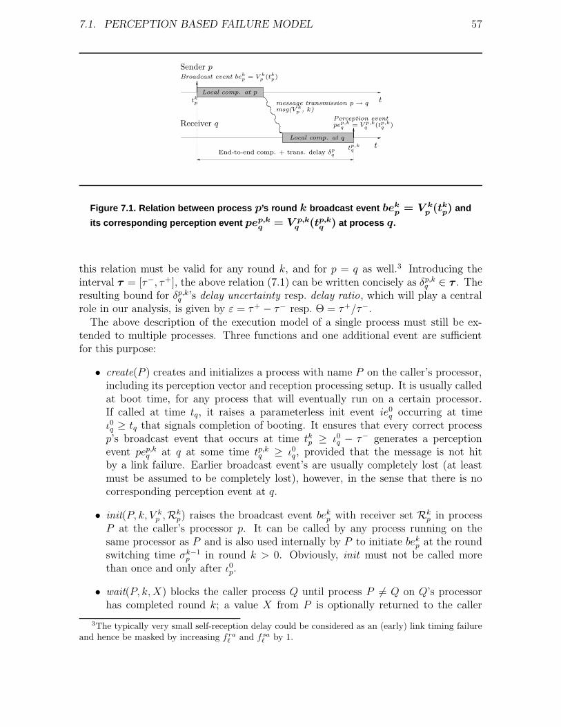
7.1. PERCEPTION BASED FAILURE MODEL 57
t
tEnd-to-end comp. + trans. delay δp
q
tkp message transmission p → q
msg(V kp , k)
Local comp. at p
Local comp. at q
Receiver q
tp,kq
Sender p
Perception eventpep,k
q = V p,kq (tp,k
q )
Broadcast event bekp = V k
p (tkp)
Figure 7.1. Relation between process p’s round k broadcast event bekp
= V kp(tk
p) and
its corresponding perception event pep,kq
= V p,kq
(tp,kq
) at process q.
this relation must be valid for any round k, and for p = q as well.3 Introducing theinterval τ = [τ−, τ+], the above relation (7.1) can be written concisely as δp,k
q ∈ τ . Theresulting bound for δp,k
q ’s delay uncertainty resp. delay ratio, which will play a centralrole in our analysis, is given by ε = τ+ − τ− resp. Θ = τ+/τ−.
The above description of the execution model of a single process must still be ex-tended to multiple processes. Three functions and one additional event are sufficientfor this purpose:
• create(P ) creates and initializes a process with name P on the caller’s processor,including its perception vector and reception processing setup. It is usually calledat boot time, for any process that will eventually run on a certain processor.If called at time tq, it raises a parameterless init event ie0
q occurring at timeι0q ≥ tq that signals completion of booting. It ensures that every correct processp’s broadcast event that occurs at time tk
p ≥ ι0q − τ− generates a perceptionevent pep,k
q at q at some time tp,kq ≥ ι0q, provided that the message is not hit
by a link failure. Earlier broadcast event’s are usually completely lost (at leastmust be assumed to be completely lost), however, in the sense that there is nocorresponding perception event at q.
• init(P, k, V kp ,Rk
p) raises the broadcast event bekp with receiver set Rk
p in processP at the caller’s processor p. It can be called by any process running on thesame processor as P and is also used internally by P to initiate bek
p at the roundswitching time σk−1
p in round k > 0. Obviously, init must not be called morethan once and only after ι0p.
• wait(P, k, X) blocks the caller process Q until process P 6= Q on Q’s processorhas completed round k; a value X from P is optionally returned to the caller
3The typically very small self-reception delay could be considered as an (early) link timing failureand hence be masked by increasing f ra
` and fsa` by 1.
58 CHAPTER 7. BOOTING CLOCK SYNCHRONIZATION
upon unblocking. Note that this operation does not affect process P ’s executionand may require some memory if P terminates round k before wait is called.
In the pseudo code employed for the description of our algorithms, a more high-levelway of expressing concurrency will usually be used:
cobegin
block 1 ...
block k
coend
is a concise description of k concurrent processes, each executing one block i.
7.1.2 Model of the Startup Phase
At the very beginning all processes are down. Every message that arrives at a processwhile it is down is lost, and no messages are sent by such a process. Note carefullythat we do not even allow spurious messages from a down process or any of its linkshere. Correct processes boot at unknown times that cannot be bounded a priori.
During startup, a correct process goes through the following sequence of operatingmodes:
1. down: A process remains down when it has not been created yet or has notcompleted booting. Messages that drop in while a process is down are usuallycompletely lost, i.e., do not generate a corresponding perception event.
2. up: A process q gets up when it has completed booting, at time ι0q. Recallthat every correct process p’s broadcast event that occurs at time tk
p ≥ ι0q − τ−
generates a perception event pep,kq at q at some time tp,k
q ≥ ι0q, provided that themessage is not hit by a link failure.
(a) passive: A process that just got up performs an algorithm dependent initial-ization phase, where it is called passive. As the first action in passive mode,a process typically sends a special join message to all its peers. The first re-ception of a join message from some process p causes the receiver to send analgorithm-dependent reply message to p (point-to-point); subsequent joinmessages from the same sender are usually ignored.
(b) active: A process that has completed its initialization phase is called active.
Remark In case of the algorithm of Figure 7.4, for example, a passive process broad-casts join—namely, (round 0), in order to get the last (round k) message of everypeer—and participates in the algorithm as in active mode. It need not satisfy theclock synchronization conditions (π) and (α) from Definition 3 while passive, however.The transition to active mode occurs when the process can be sure that it is withinthe synchronization precision Dboot.
7.1. PERCEPTION BASED FAILURE MODEL 59
The communication pattern for joining is obviously different from ordinary rounds.Whereas join is broadcast by a single joining process p, the replies are typically sentback by all peers via point-to-point messages. All the processes’ join can be consideredas a special booting round’s messages, however, so both execution model and failuremodel apply to join as for any round k message. Response messages are different,however. Although compatibility with our execution model is maintained by assumingRresp
q = p and Srespp = Π, we need some additional assumptions with respect to our
failure model.Since the semantics of response messages are algorithm dependent, it does not make
sense to define a generic model here. Basically, the joiner p must be provided with suf-ficient information to construct an internal state that is equivalent—in some algorithmdependent sense—to the state it would have had if it had not missed earlier messagesdue to late booting. This is a demanding requirement, however, since e.g. failures thatoccurred before p got up must be taken into account.
In case of the clock synchronization algorithm of Section 7.2, for instance, any pro-cess s that successfully received p’s join responds by retransmitting4 the last sent(round ks). Retransmissions must happen in a way, however, which lets the resultingperception matrices maintain compliance with our failure model. For example, if arbi-trary link failures in process s’s original round ks broadcast already caused f ra
` receiversq 6= p to deliver faulty round ks perceptions V s,ks
q , it must not happen that s’s responsemessage to p’s join suffers from an arbitrary link failure as well. Response messagesmay hence be viewed as messages belonging to the original round k broadcast here,which are deferred until the appropriate receiver is up. As in case of messages withhistory h > 0, perceptions recovered via response messages are usually time faulty,however (see Remark 4 on Definition 10).
7.1.3 Physical Failure Model
Our physical failure model basically5 assumes that at most fa, fs, fo and fc processorsmay be arbitrary, symmetric, omission, and clean crash faulty during any single round.Clean crash faulty processes may be mute to all receiving processes (consistently) insome round, omission faulty processes may fail to send the correct message to anarbitrary subset of the receivers (inconsistently). Symmetric failures allow a processto disseminate an erroneous value consistently, whereas arbitrary faulty processes mayeven exhibit Byzantine behavior.
Since we will often establish uniform results (which also hold for processors withbenign failures, namely, omission and clean crash faulty processes unless they have
4These retransmissions may cause the arrival of two round k messages from the same sender, whichis usually considered an error in our execution model, recall Section 7.1.1. This is of course not truehere, so we just assume that the first perception entered into some round k perception vector isretained—and not overwritten by some error value—when a second round k message drops in.
5In the fully-fledged physical failure model [87], it is differentiated between the number of physicalfailures φav , φsv , . . . and the number of perceptions failures fa, fs, . . . for generality. More specifically,formulas like fa = φav for the perception failure numbers, given the physical failure numbers, areprovided when mapping the the physical failure model to the perception failure model.
60 CHAPTER 7. BOOTING CLOCK SYNCHRONIZATION
crashed), we will use the term obedient process to denote non-faulty, omission, andclean crash faulty processes that are still alive at the point of observation.
As far as link failures are concerned, every receiving process may experience at mostf r
` link failures affecting different peers in the reception of every round, with at mostf ra
` ≤ f r` arbitrary time/value faulty ones (producing early or late message receptions
and/or faulty values). Similarly, every sending process may generate at most f s` link
failures when sending a message to all its peers per round, with at most f sa` ≤ f s
`
arbitrary time/value faulty ones among those. Assigning different numbers of sendand receive link failures is useful for modeling certain restricted process failures [90];usually, however, f r
` = f s` = f` and f ra
` = f sa` = f a
` . As long as processes do notexceed those limits, they need not be considered (process) faulty. Further details willbe provided in the next section.
Remark Note that we stick to Schmid’s [87] original definition of the fault model:Crash failures in the physical failure model are equivalent to clean-crash failures inSection 6.4.1. The (asymmetric) crash faults of Section 6.4.2 on the other hand mustbe modeled as omission faulty here.
7.1.4 Perception Failure Model
Consider the round k perception vector Vkq (t)—observed at some real-time t—of a
well-behaved process q. Our execution model implies that Vkq (t) is monotonic in time,
in the sense that |Vkq (t + ∆t)| ≥ |Vk
q (t)| for any ∆t ≥ 0, since perceptions are onlyadded. Moreover, since the value V k+1
q to be broadcast in the next round k + 1 iscomputed solely from Vk
q := Vkq (σk
q ) and q’s local state at the round switching timeσk
q , it is obvious that, ultimately, only the failures in the perceptions present at therespective round switching times count. Timing failures are no longer visible here (butwill probably affect σk
q , recall Section 7.1.1), since a message that did not drop in byσk
q at process q just results in V p,kq = ∅. Consequently, the resulting perception failure
model is much simpler than the physical one and therefore more suitable for analyzingan algorithm’s fault-tolerance properties.
Our formalization hence rests upon the n × n perception matrix Vk(t)6 of round kperceptions observed at the same arbitrary real-time t—typically some process’s roundswitching time—at all processes:
V(t) =
V1(t)V2(t)
...Vn(t)
=
V 11 V 2
1 . . . V n1
V 12 V 2
2 . . . V n2
......
......
V 1n V 2
n . . . V nn
t
(7.2)
Note that V(t) is in fact a quite flexible basis for our failure model, since different“views” of the state of the distributed computation can be produced easily by choosinga suitable t.
We distinguish the following failure modes for single perceptions in V(t) in our per-ception failure model:
6We will subsequently suppress the round number k in quantities like Vk(t) for brevity.
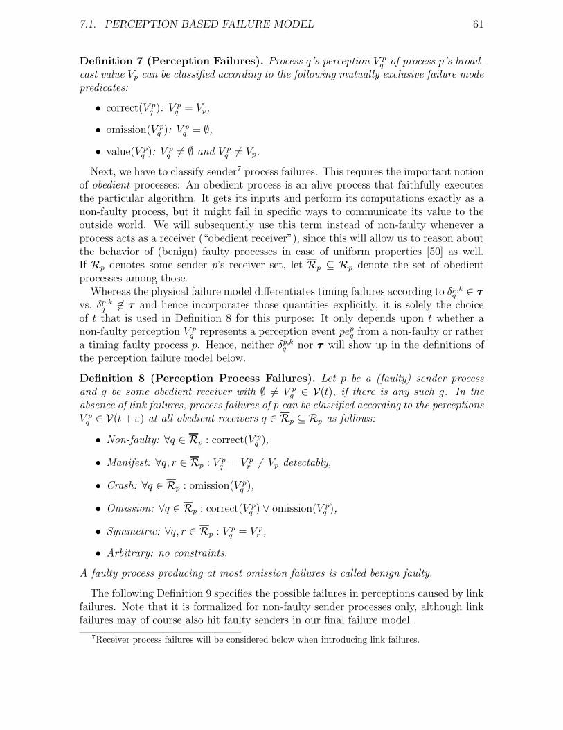
7.1. PERCEPTION BASED FAILURE MODEL 61
Definition 7 (Perception Failures). Process q’s perception V pq of process p’s broad-
cast value Vp can be classified according to the following mutually exclusive failure modepredicates:
• correct(V pq ): V p
q = Vp,
• omission(V pq ): V p
q = ∅,
• value(V pq ): V p
q 6= ∅ and V pq 6= Vp.
Next, we have to classify sender7 process failures. This requires the important notionof obedient processes: An obedient process is an alive process that faithfully executesthe particular algorithm. It gets its inputs and perform its computations exactly as anon-faulty process, but it might fail in specific ways to communicate its value to theoutside world. We will subsequently use this term instead of non-faulty whenever aprocess acts as a receiver (“obedient receiver”), since this will allow us to reason aboutthe behavior of (benign) faulty processes in case of uniform properties [50] as well.If Rp denotes some sender p’s receiver set, let Rp ⊆ Rp denote the set of obedientprocesses among those.
Whereas the physical failure model differentiates timing failures according to δp,kq ∈ τ
vs. δp,kq 6∈ τ and hence incorporates those quantities explicitly, it is solely the choice
of t that is used in Definition 8 for this purpose: It only depends upon t whether anon-faulty perception V p
q represents a perception event pepq from a non-faulty or rather
a timing faulty process p. Hence, neither δp,kq nor τ will show up in the definitions of
the perception failure model below.
Definition 8 (Perception Process Failures). Let p be a (faulty) sender processand g be some obedient receiver with ∅ 6= V p
g ∈ V(t), if there is any such g. In theabsence of link failures, process failures of p can be classified according to the perceptionsV p
q ∈ V(t + ε) at all obedient receivers q ∈ Rp ⊆ Rp as follows:
• Non-faulty: ∀q ∈ Rp : correct(V pq ),
• Manifest: ∀q, r ∈ Rp : V pq = V p
r 6= Vp detectably,
• Crash: ∀q ∈ Rp : omission(V pq ),
• Omission: ∀q ∈ Rp : correct(V pq ) ∨ omission(V p
q ),
• Symmetric: ∀q, r ∈ Rp : V pq = V p
r ,
• Arbitrary: no constraints.
A faulty process producing at most omission failures is called benign faulty.
The following Definition 9 specifies the possible failures in perceptions caused by linkfailures. Note that it is formalized for non-faulty sender processes only, although linkfailures may of course also hit faulty senders in our final failure model.
7Receiver process failures will be considered below when introducing link failures.
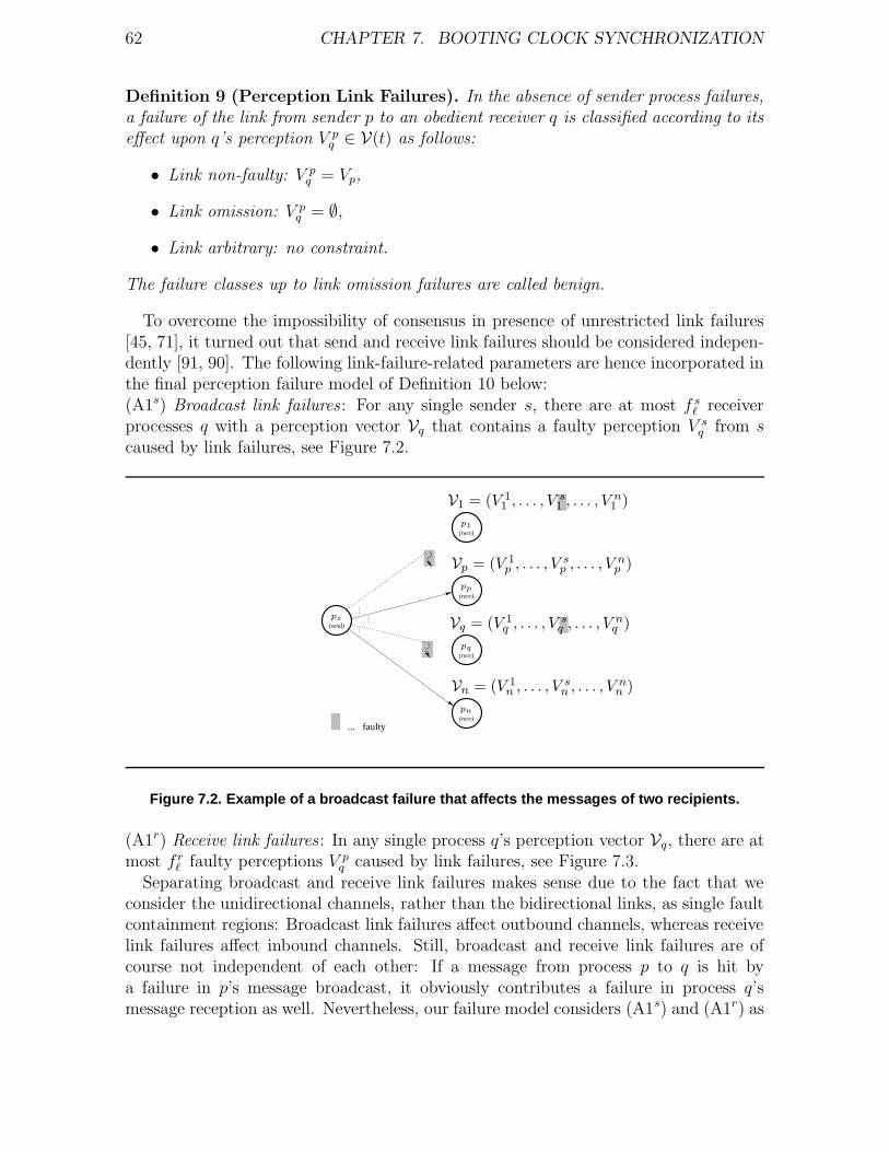
62 CHAPTER 7. BOOTING CLOCK SYNCHRONIZATION
Definition 9 (Perception Link Failures). In the absence of sender process failures,a failure of the link from sender p to an obedient receiver q is classified according to itseffect upon q’s perception V p
q ∈ V(t) as follows:
• Link non-faulty: V pq = Vp,
• Link omission: V pq = ∅,
• Link arbitrary: no constraint.
The failure classes up to link omission failures are called benign.
To overcome the impossibility of consensus in presence of unrestricted link failures[45, 71], it turned out that send and receive link failures should be considered indepen-dently [91, 90]. The following link-failure-related parameters are hence incorporated inthe final perception failure model of Definition 10 below:(A1s) Broadcast link failures: For any single sender s, there are at most f s
` receiverprocesses q with a perception vector Vq that contains a faulty perception V s
q from scaused by link failures, see Figure 7.2.
(recv)
... faulty
(send)
(recv)
(recv)
(recv)
Vq = (V 1q , . . . , V s
q , . . . , V nq )
V1 = (V 11 , . . . , V s
1 , . . . , V n1 )
p1
ps
Vp = (V 1p , . . . , V s
p , . . . , V np )
Vn = (V 1n , . . . , V s
n , . . . , V nn )
pq
pp
pn
Figure 7.2. Example of a broadcast failure that affects the messages of two recipients.
(A1r) Receive link failures: In any single process q’s perception vector Vq, there are atmost f r
` faulty perceptions V pq caused by link failures, see Figure 7.3.
Separating broadcast and receive link failures makes sense due to the fact that weconsider the unidirectional channels, rather than the bidirectional links, as single faultcontainment regions: Broadcast link failures affect outbound channels, whereas receivelink failures affect inbound channels. Still, broadcast and receive link failures are ofcourse not independent of each other: If a message from process p to q is hit bya failure in p’s message broadcast, it obviously contributes a failure in process q’smessage reception as well. Nevertheless, our failure model considers (A1s) and (A1r) as
7.1. PERCEPTION BASED FAILURE MODEL 63
(send)
(send)
(send)
(send)
(recv)
... faulty
Vr = (V 1r , . . . , V p
r , V qr , . . . , V n
r )
pr
p1
pp
pq
pn
Figure 7.3. Example of a receive failure that involves the messages from two senders.
independent of each other and of process failures, for any process in the system and anybroadcast/reception. Only the model parameters f s
` and f r` cannot be independently
chosen (without restricting the link failure patterns), since the system-wide number ofbroadcast and receive link failures must of course match. Hence, f s
` = f r` = f` is the
most natural choice, although other settings can also be considered [90].Note carefully that we allow every process in the system to commit up to f s
` broadcastand up to f r
` receive link failures in every round, without considering the process asfaulty in the usual sense. In addition, the particular links actually hit by a link failuremay be different in different rounds. A process must be considered (omission) faulty,however, if it exceeds its budget f s
` of broadcast link failures in some round. Note thata process that experiences more than f r
` receive link failures in some round must ingeneral be considered (arbitrary) faulty, since it might be unable to correctly followthe algorithm after such an event.
The following Definition 10 contains the complete perception based failure model,which just specifies the properties of any round’s perception matrix VR(t). Note care-fully that this definition is valid for arbitrary times t, including those where the per-ceptions from some senders did not yet arrive (and are hence ∅).
Definition 10 (Asynchronous Perception Failure Model). Let Vk(t) be theround k perception matrix of an asynchronous system of processes running on differ-ent processors that comply to our execution model. For any obedient receiver q, it isguaranteed that V p,k
q = ∅ if p 6∈ Skq or if V p,k
q was not received by time t. Moreover:
(P1) There are at most fa, fs, fo, fc, and fm columns in Vk(t) that may correspondto arbitrary, symmetric, omission, crash, and manifest faulty processes and mayhence contain perceptions V p,k
q according to Definition 8.
(A1s) In every single column p, at most f s` perceptions V p,k
q ∈ Vk(t) corresponding to
obedient receivers q ∈ Rk
p ⊆ Rkp may differ from the ones obtained in the absence
64 CHAPTER 7. BOOTING CLOCK SYNCHRONIZATION
of broadcast link failures. At most f sa` ≤ f s
` of those perceptions may be linkarbitrary faulty.
(A1r) In every single row q corresponding to an obedient receiver, at most f r` of the
perceptions V p,kq ∈ Vk(t) corresponding to senders p ∈ Sk
q may differ from theones obtained in the absence of receive link failures. At most f ra
` ≤ f r` of those
may be link arbitrary faulty.
(A2) Process q can be sure about the origin p of V p,kq ∈ Vk(t).
(A3) ∅ 6= V p,kq ∈ Vk(t) ⇒ ∅ 6= V p,k
r ∈ Vk(t+ε) for every non-faulty sender p connectedto obedient receivers q and r via non-faulty links.
Remarks
1. The effects of process failures (P1) and link failures (A1s), (A1r) are consideredorthogonal; it can hence happen that a link failure hits a perception originatingfrom a faulty sender process. This is also true for manifest and clean crashfailures, where link arbitrary failures could create non-empty perceptions at somereceivers.
2. (P1) implies that our perception failure model is compatible with traditionalprocess failure models. For example, fa Byzantine faulty processes can gener-ate inconsistently faulty perceptions only in the fa columns they correspond to.Hence, all existing lower bounds and impossibility results, like n ≥ 3fa + 1 forconsensus in presence of fa arbitrary process failures [60], remain valid.
3. Analysis results under our perception failure model are automatically valid forpartially connected networks as well, since the consequences of an incompletecommunication graph can be viewed as (persistent) link omission failures. How-ever, sparsely connected graphs and, in particular, partitioned ones cannot bemodeled, cp. [90, Thm.3.2].
4. Our failure model also allows arbitrary resp. symmetric faulty processes to com-mit an early/late timing failure inconsistently resp. consistently (within ε). Nei-ther omission faulty nor clean crash faulty processes may generate time-faultyperceptions in case of no history (h = 0). In case of messages with history or re-sponses to join-messages, however, the latter cannot usually be guaranteed: Justtake an omission faulty process s, for example, which omits sending a round kmessage to p but not to q. If this process sends a round k + 1 message to pin the next round, it also generates a round k perception V s,k
p at p. AlthoughV s,k
p = V s,kq , the former is of course time faulty since it arrived too late w.r.t.
the sender’s proper round k’s broadcast event. Hence, any type of benign pro-cess failure may result in a timing failure in case of h > 0 and must hence beaccounted for in fs or fa. Note that the latter is not required for the algorithmstudied in this paper, since late timing failures are no more severe than omissionsfor the algorithm of Figure 7.4.
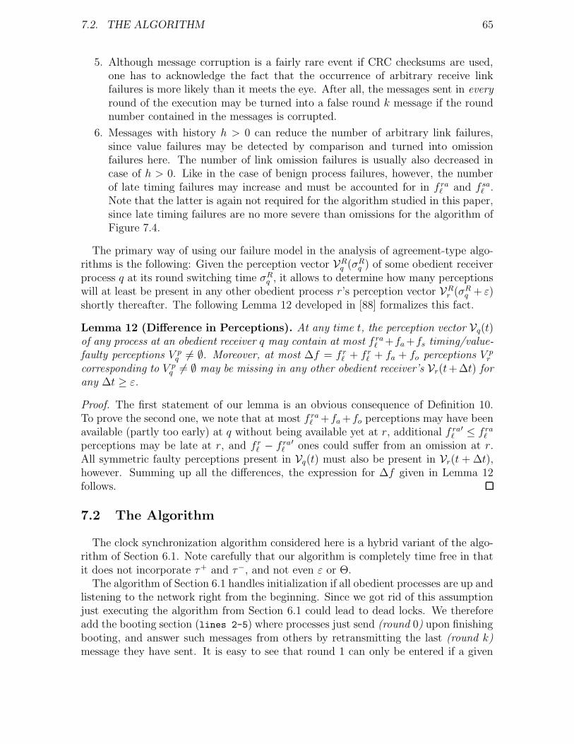
7.2. THE ALGORITHM 65
5. Although message corruption is a fairly rare event if CRC checksums are used,one has to acknowledge the fact that the occurrence of arbitrary receive linkfailures is more likely than it meets the eye. After all, the messages sent in everyround of the execution may be turned into a false round k message if the roundnumber contained in the messages is corrupted.
6. Messages with history h > 0 can reduce the number of arbitrary link failures,since value failures may be detected by comparison and turned into omissionfailures here. The number of link omission failures is usually also decreased incase of h > 0. Like in the case of benign process failures, however, the numberof late timing failures may increase and must be accounted for in f ra
` and f sa` .
Note that the latter is again not required for the algorithm studied in this paper,since late timing failures are no more severe than omissions for the algorithm ofFigure 7.4.
The primary way of using our failure model in the analysis of agreement-type algo-rithms is the following: Given the perception vector VR
q (σRq ) of some obedient receiver
process q at its round switching time σRq , it allows to determine how many perceptions
will at least be present in any other obedient process r’s perception vector VRr (σR
q + ε)shortly thereafter. The following Lemma 12 developed in [88] formalizes this fact.
Lemma 12 (Difference in Perceptions). At any time t, the perception vector Vq(t)of any process at an obedient receiver q may contain at most f ra
` +fa +fs timing/value-faulty perceptions V p
q 6= ∅. Moreover, at most ∆f = f r` + f r
` + fa + fo perceptions V pr
corresponding to V pq 6= ∅ may be missing in any other obedient receiver’s Vr(t+∆t) for
any ∆t ≥ ε.
Proof. The first statement of our lemma is an obvious consequence of Definition 10.To prove the second one, we note that at most f ra
` +fa +fo perceptions may have beenavailable (partly too early) at q without being available yet at r, additional f ra
`′ ≤ f ra
`
perceptions may be late at r, and f r` − f ra
`′ ones could suffer from an omission at r.
All symmetric faulty perceptions present in Vq(t) must also be present in Vr(t + ∆t),however. Summing up all the differences, the expression for ∆f given in Lemma 12follows.
7.2 The Algorithm
The clock synchronization algorithm considered here is a hybrid variant of the algo-rithm of Section 6.1. Note carefully that our algorithm is completely time free in thatit does not incorporate τ+ and τ−, and not even ε or Θ.
The algorithm of Section 6.1 handles initialization if all obedient processes are up andlistening to the network right from the beginning. Since we got rid of this assumptionjust executing the algorithm from Section 6.1 could lead to dead locks. We thereforeadd the booting section (lines 2-5) where processes just send (round 0) upon finishingbooting, and answer such messages from others by retransmitting the last (round k)message they have sent. It is easy to see that round 1 can only be entered if a given
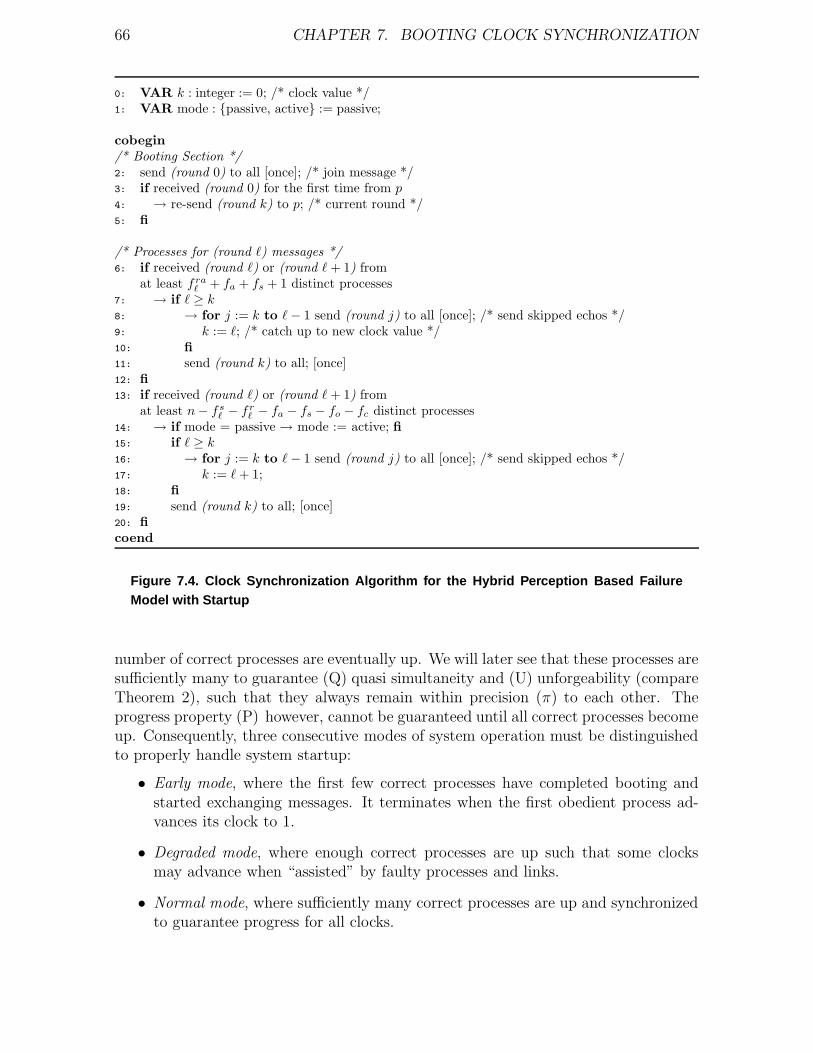
66 CHAPTER 7. BOOTING CLOCK SYNCHRONIZATION
0: VAR k : integer := 0; /* clock value */1: VAR mode : passive, active := passive;
cobegin
/* Booting Section */2: send (round 0) to all [once]; /* join message */3: if received (round 0) for the first time from p4: → re-send (round k) to p; /* current round */5: fi
/* Processes for (round `) messages */6: if received (round `) or (round ` + 1) from
at least f ra` + fa + fs + 1 distinct processes
7: → if ` ≥ k8: → for j := k to ` − 1 send (round j) to all [once]; /* send skipped echos */9: k := `; /* catch up to new clock value */10: fi
11: send (round k) to all; [once]12: fi
13: if received (round `) or (round ` + 1) fromat least n − f s
` − fr` − fa − fs − fo − fc distinct processes
14: → if mode = passive → mode := active; fi
15: if ` ≥ k16: → for j := k to ` − 1 send (round j) to all [once]; /* send skipped echos */17: k := ` + 1;18: fi
19: send (round k) to all; [once]20: fi
coend
Figure 7.4. Clock Synchronization Algorithm for the Hybrid Perception Based FailureModel with Startup
number of correct processes are eventually up. We will later see that these processes aresufficiently many to guarantee (Q) quasi simultaneity and (U) unforgeability (compareTheorem 2), such that they always remain within precision (π) to each other. Theprogress property (P) however, cannot be guaranteed until all correct processes becomeup. Consequently, three consecutive modes of system operation must be distinguishedto properly handle system startup:
• Early mode, where the first few correct processes have completed booting andstarted exchanging messages. It terminates when the first obedient process ad-vances its clock to 1.
• Degraded mode, where enough correct processes are up such that some clocksmay advance when “assisted” by faulty processes and links.
• Normal mode, where sufficiently many correct processes are up and synchronizedto guarantee progress for all clocks.
7.3. MAPPING TO THE PERCEPTION BASED EXECUTION MODEL 67
Note carefully that it is impossible for any process in the system to delimit the exactborders between those modes from local information.
In order to add system startup handling to the original clock synchronization algo-rithm, join messages and an additional if-clauses are required. First of all, a newlybooted process must tell all others that it is up now and must learn their current clockvalues. This is accomplished by means of join messages, as introduced in Section 7.1.2:Every process p sends join = (round 0) as the very first message after having com-pleted booting. Every process q that receives this message replies by retransmitting itspreviously sent (round k) message (lines 2-5). This ensures that p will eventually getsufficiently many messages—which may have been lost while it was down—to triggerthe catch-up rule described below.
In order to ensure that a late starter can catch-up it must receive f ra` + fa + fs + 1
messages for a single round from distinct processes (line 6). Due to (Q) we can onlyguarantee that correct processes remain within two rounds. This is why we introducedmessages with history size h = 1.
Moreover, due to failures or a large group of simultaneous late joiners, the firstround an initializing process might reach by the catch-up rule could be arbitrarilysmall. This would violate the precision requirement, however. We therefore assumethat only active, but not passive processes, must satisfy (π). A passive process switchesto active mode when it has sufficient evidence that its local round number is withinprecision Dboot of the clocks of the other correct active processes in the system. This isaccomplished by the second if-clause (line 13), which triggers when sufficiently many(round `) messages have been received. We will show in Section 7.4 that any such `can be guaranteed to be sufficiently close to the maximum correct clock value in thesystem.
In the following sections, we will prove that our algorithm satisfies the clock syn-chronization properties (π) and (α) – (π) during whole system operation and (α) whensufficiently many correct processes are up. In Section 7.3, we will see how its executionmatches the execution model of Section 7.1.1. The analysis starts with Section 7.4,where we explore how our algorithm behaves in early and degraded mode, i.e. whennot sufficiently many processes are up to guarantee progress of the clocks. Section 7.5deals with the transition between degraded and normal mode, which takes place whenlate processes join the system.
7.3 Mapping to the Perception based Execution Model
The algorithm is given in an event based notion that consists of the three outermostif-statements, numbered from the zero-th if (line 2) up to the second if (line 13). Thevariable k provides the clock value Cp(t) of the processor p that executes the algorithm.In order to be able to analyze our algorithm under the perception based failure modelof Definition 10, we must show that its execution complies to the execution modelof Section 7.1.1. Every execution of our algorithm can in fact be described by thefollowing process running on every processor p:
Infinitely many single-round processes L, L ≥ 0, where process L processes (round `)
68 CHAPTER 7. BOOTING CLOCK SYNCHRONIZATION
messages for ` = L in the perception vector V `p. All those processes must be active
concurrently right from the start and can terminate after execution of line 13. Notethat they can be viewed as a way of concurrently executing all rounds of a singlemultiple-round process.
In order formally model the fact that computations are actually triggered uponarrival of (round x) or (round x + 1) in our algorithm, we use messages with historysize h = 1. For example, when an (round k + 1) message from process p arrives atq in case of h = 1, both the perception V p,k+1
q and, provided that still V p,kq = ∅, the
perception V p,kq is filled. Hence, the above processes can act upon a single perception
vector Vkq as required by our execution model, yet process messages (round k) and
(round k + 1).
As in Definition 2 it is possible also for the perception based failure model to definean effective uncertainty ratio Ω. In order to do so we give the following definition andlemma.
Definition 11 (Short Transmission Times). Let q be any obedient processes. Con-sidering a fixed obedient process q, τ−
q is the n − f s` − f ra
` − f r` − 2fa − 2fs − fo − fc
smallest δpq for all messages sent by obedient processes p which are used to enable anevent at q at real-time t. τf is the smallest τ−
q for any obedient process q.
The term n− f s` − f ra
` − f r` − 2fa − 2fs − fo − fc accounts for the minimal number of
messages by obedient processes which is required by any obedient process—executingthe algorithm given in Figure 7.4—to advance its clock by line 13.
Lemma 13 (Incoming Messages). If a correct process receives messages by at leastn − f s
` − f ra` − f r
` − 2fa − 2fs − fo − fc distinct obedient processes by time t, then atleast one message from these processes was sent by time t − τf.
Proof. Follows from Definition 1.
Definition 12 (Hybrid Effective Uncertainty Ratio). The smallest value of theuncertainty ratio which may be considered in the late binding process is Ω = τ +/τf.
7.4 From Early to Degraded Mode
Before considering the full system startup scenario, we will study the algorithm ofFigure 7.4 in a system of n ≥ f s
` +2f ra` +2f r
` +3fa+2fs+2fo+fc+1 processes,8 where afixed but arbitrary number 0 ≤ nup(K) ≤ n of processes have completed booting whenthe messages from the first obedient process that started some round K may arrive.Note that all those nup(K) processes can receive all messages for ticks k ≥ K fromeach other (except faulty ones, of course). The special case nup(0) = n describes the
8Incorporating f s` in our algorithm is only required to guarantee liveness in the transition from
degraded to normal mode (Theorem 22 and Theorem 24); it accounts for send link failures in join-messages of late starters. Consequently, most of our results—in particular, the ones of this section—hold when setting f s
` = 0 in Figure 7.4 and in our formulas (despite of f r` > 0) as well.
7.4. FROM EARLY TO DEGRADED MODE 69
situation where all processes must be up and running right from the very beginning,i.e., where system startup is ignored [70, 95, 86]. The case nup(1) < n will be used todescribe the behavior of our algorithm during (the beginning of) degraded mode.
We start with some frequently used definitions and lemmas, which apply to anyoperation mode. Note that a passive process p’s local clock Cp(t) refers to its currentround number k (see Figure 7.4) at time t in our analysis; terms like p’s clock valueand “p sets its clock” are hence meaningful for both active and passive processes. Still,the clock synchronization properties need only hold for active processes. Of particularimportance is the maximum clock value of all obedient processes in the system, whichwill be used as the ”reference time” in our precision analysis.
Definition 13 (Maximum Clock Value). Consider some real-time t.
• Cmax(t) is the maximum of the local clocks of all obedient processes that are upat time t.
• σk−1first = σk−1
p ≤ t denotes the real-time when the first obedient process p sets its
local clock to k = Cmax(t); σ−1first is the time when the first obedient process has
completed booting. Note that p’s clock value, and hence Cmax, is defined to be kat time σk−1
first, and k − 1 at σk−1first − ε for any infinitesimally small ε > 0.
The maximum set of obedient processes that did not miss any tick k message from eachother (except the ones missing due to process or link failures, of course) is denoted byPup(k), with nup(k) = |Pup(k)|.
The following Lemma 14 reveals a few straightforward properties about messagessent by correct9 processes.
Lemma 14 (Message Generation). Consider any correct process p executing thealgorithm of Figure 7.4. If p reached clock value k > 0 by time t, it must have sent(round k′) for all 0 ≤ k′ ≤ k − 1 by time t.
Proof. Consider the sequence of values cmm≥0, assigned to p’s clock variable at real-times tmm≥0. Using induction on m, we will show that p must have emitted (round `′)for all 0 ≤ `′ ≤ cm by time tm. Since it is obvious from Figure 7.4 that cm can only bemonotonically increasing, our lemma then follows immediately.
For the basis m = 0, obviously c0 = 0 and the claim is void since no (round) messageneeds to have been sent by t0. Assuming now that the claim holds for m−1 ≥ 0, i.e. all(round `′) for 0 ≤ `′ ≤ cm−1 have been sent by time tm−1 when p’s clock is set to cm−1,we have to show that the claim holds for m as well: Two cases must be distinguishedhere, according to whether setting p’s clock to cm occurs via line 6 or line 13.
If p sets its clock via line 13 in in Figure 7.4, we must obviously have cm = cm−1 +1.Since triggering of line 13 implies triggering of line 6, (round cm−1) = (round cm−1)must have been sent by time tm. Combining this with the induction hypothesis, theclaim follows immediately.
9Transmission of messages of obedient process q are guaranteed to be successful only if q is correct.
70 CHAPTER 7. BOOTING CLOCK SYNCHRONIZATION
If p sets its clock to cm via line 6, it sends (echo, l′′) for cm−1 ≤ l′′ ≤ cm by line 8;note that (echo, cm−1) is of course only emitted here if this has not happened earlier.Combining this with the induction hypothesis, our claim follows also in this case.
The following lemma shows that progress of Cmax(t) is only possible via line 13.
Lemma 15 (2nd if). The first obedient process that sets its clock to tick k = Cmax(t) >0 by time t must do so by line 13.
Proof. By contradiction. Assume that the first obedient process p sets its clock tok = Cmax(t) at instant t by line 6. At least one obedient process must have sent amessage for a tick ` ≥ k to enable this rule at p. Since obedient processes only sendmessages for ticks less or equal their local clock value, at least one must already havehad a clock value ` ≥ k at instant t. This contradicts p to be the first one that reachesclock value k.
The following Lemma 16 shows that processes which completed booting early enoughcan be guaranteed to be in Pup(k), since they must have got all tick k messages fromother obedient processes (except messages hit by failures). Bear in mind, however, thatearly booting is not the only only way of ensuring inclusion in Pup(k). A late startingprocess p may also achieve p ∈ Pup(k) via the join-protocol even though it completesbooting after time σk−1
first + τ−.
Lemma 16 (Booting Times). Any obedient process p that is up by time σk−1first + τ−
satisfies p ∈ Pup(k).
Proof. Since the first obedient process that emits a tick k message does so not earlierthan time σk−1
first, according to our algorithm in Figure 7.4 and Lemma 15, no obedient
process p can receive such a message before time σk−1first + τ−. Since p is up by that
time, it will hence receive all tick ` ≥ k messages from correct processes.
The following Theorem 18 is the first major result of this section. It shows thatthe clocks of obedient processes obey two properties, namely, uniform unforgeability(U), and uniform quasi simultaneity (Q) – in concordance with Section 6.1. Theseproperties are weak in the sense that they suffice to ensure (π) but are to weak toguarantee (α). This is due to the small number of processes that participate duringbooting and the impossibility results [30] on the minimal number of processes whichare required to guarantee (π) and (α).
Theorem 18 (Weak Clock Synchronization Properties). For n ≥ f s` + 2f ra
` +2f r
` + 3fa + 2fs + 2fo + fc + 1, the algorithm from Figure 7.4 achieves
(U) Uniform Unforgeability. If no obedient process sets its clock to k by time t, thenno obedient process sets its clock to k + 1 by time t + τf or earlier.
(Q) Uniform Quasi Simultaneity. For any k ≥ 1, if an obedient process sets its clockto k at time t, then, by time t + ε, every obedient process ∈ Pup(k − 1) sets itsclock at least to k − 1 and, if correct, sends (round k − 1).
7.4. FROM EARLY TO DEGRADED MODE 71
Proof. Uniform Unforgeability. Setting the clock value can be done by (1) the line 13
or (2) line 6. The proofs are by contradiction.Assume (1) that there is an obedient process p that sets its clock to k+1 before instant
t+ τf using line 13. This implies |Vkp (t+ τf)| ≥ n−f s
` −f ra` −f r
` −2fa −2fs−fo −fc ≥2f ra
` +f r` +2fa+fo+fs+1. Since, according to Lemma 12, only at most f ra
` +fa+fs of thecorresponding (round k) perceptions may be due to messages produced by arbitraryreceive link failures and time/value-faulty processes, at least one obedient process qmust have sent (round k) for k ∈ k, k+1 before time t+τf (according to Lemma 13),which contradicts the assumption of unforgeability.
Assume (2) that there is an obedient process p that sets its clock to k + 1 beforeinstant t + τf using line 6. Process p does so because |V l
p(t + τf)| ≥ f ra` + fa + fs + 1
for some l ≥ k + 1. That is, at least one (round l) message, l ∈ l, l + 1, must havebeen sent by an obedient process q before t. l > k and messages for tick l are sent byan obedient process only after tick k messages. But by assumption of (U), no tick kmessage was sent before t, which again provides the required contradiction.
Uniform Quasi Simultaneity. Assume first that k = Cmax(t). If the obedient processp that advanced its clock to k by assumption used line 13, then |V (k−1)
p (t)| ≥ 2f ra` +
f r` + 2fa + fo + fs + 1. Hence, the perception vector for tick k − 1 at any obedient
process q ∈ Pup(k − 1) at time t + ε must satisfy |V (k−1)q (t + ε)| ≥ f ra
` + fa + fs + 1according to Lemma 12.10 It follows that every obedient process ∈ Pup(k− 1) achievessufficient evidence in line 6 to catch-up to round k− 1 (if it has not already done so).This fact (or Lemma 14 if p has already reached an even larger clock value ≥ k byt + ε) guarantees that (round k − 1) is sent by time t + ε.
If, on the other hand, the obedient process p advanced its clock to k by line 6, theremust be a process p′ that set its clock to k by line 13 earlier according to Lemma 15.Using p′ in the above argument establishes (Q) in this case as well.
If k < Cmax(t), then at least one obedient process has already set its clock to l > kat some time t′ ≤ t using line 13. We have shown in the previous paragraph that allobedient processes ∈ Pup(k − 1) must set their clocks to l − 1 (and hence at least tok − 1) by time t′ + ε (and hence by time t + ε) as asserted.
Since (U) and (Q) are satisfied, Lemma 3 and Lemma 4—derived in Section 6.1—hold as well. These lemmas will be used in the following analysis.
The following two technical Lemmas 17 and 18 are the major tools in our precisionanalysis. Both lemmas—and hence all the results built upon those—actually hold forevery algorithm that satisfies uniform unforgeability (U) and uniform quasi simultane-ity (Q). Lemma 18 bounds the maximum real-time difference between any obedientprocess’s clock and Cmax (i.e., the fastest obedient process) at about the same clocktime. Note carefully that it actually holds for any k′ ≥ k and hence for any t ≥ σk
first,since p ∈ Pup(k) implies p ∈ Pup(k
′).
10If n is increased, |V(k−1)q
′
(t + ε)| increases accordingly. This fact will be used for ensuring quasisimultaneity (Q) despite of some missing (round k − 1) due to send link failures: By adding anotherfs
` to n, the at most f s` lost join-messages of a late starter p, which may lead to the lack of up to f s
`
responses (round k − 1) at p, can be masked transparently, see the proof of Theorem 22.
72 CHAPTER 7. BOOTING CLOCK SYNCHRONIZATION
Lemma 17 (Real-Time Bounds). For any obedient process p ∈ Pup(k) where k+1 =Cmax(t) such that σk
first ≤ t < σk+1first, the following holds:
σk−1p ≤ σk
first + ε (7.3)
Cp(t + ε) ≥ Cp(σk−1p ) = Cmax(σ
kfirst) − 1 = Cmax(t) − 1 (7.4)
Moreover, if p is correct, it is guaranteed to send (round k) by time t + ε.
Proof. According to (Q) in Theorem 18, all obedient processes ∈ Pup(k), and hencealso p, must set their clocks to at least k by time σk
first + ε. (Q) hence implies (7.3)and the claimed sending of (round k).
If (7.3) holds, it follows from σkfirst ≤ t < σk+1
first that Cmax(t) = k + 1 and σk−1p ≤
σkfirst+ε ≤ t+ε. Consequently, Cp(t+ε) ≥ Cp(σ
k−1p ) = k and hence Cmax(t)−Cp(t+ε) ≤
1, which confirms (7.4).
The following lemma provides a bound for the maximum clock time difference of anyobedient process and Cmax at the same real-time. Note that the precision Dq implied byLemma 18 actually holds for any k′ ≥ k and hence for any t ≥ σk−2
p , since p ∈ Pup(k)implies p ∈ Pup(k
′).
Lemma 18 (Logical Time Bounds). For any obedient process p ∈ Pup(k), k ≥ 1,and any t′ with σk−2
p ≤ t′ < σk−1p ,
Cmax(t′) ≤ Cp(t
′) + Dq = k − 1 + Dq (7.5)
Cmax(σk−1p ) ≤ Cp(σ
k−1p ) + Dq − 1 = k − 1 + Dq (7.6)
with
Dq = bΩ + 2c. (7.7)
Proof. If Cmax never reaches k + 1, (7.5) and (7.6) hold trivially since Dq ≥ 1. Hence,suppose that Cmax reaches k+1 at time σk
first < ∞. Let t = σk−1p denote the time when
p sets its clock to k. In order to compute Cmax(t), we use Lemma 4 and our knowledgeof Cmax(t− ε) ≤ Cmax(σ
kfirst) = k + 1 due to monotonicity of Cmax in conjunction with
(7.3): From Lemma 4, we infer that Cmax(t) ≤ b t−(t−ε)τf
c + Iσ(t − ε) + Cmax(t − ε). If
σkfirst = t − ε such that t − ε is synchronized with Cmax, then Cmax(t − ε) = k + 1 and
Iσ(t − ε) = 0 according to Definition 6. If, on the other hand, σkfirst > t − ε, then
Cmax(t − ε) = k and Iσ(t − ε) = 1. In both cases, Iσ(t − ε) + Cmax(t − ε) = k + 1 andhence Cmax(t) ≤ b ε
τfc+ k + 1 ≤ bΩ + 2c+ k− 1. As Cmax(t
′) ≤ Cmax(t) since t′ < t and
Cp(t′) = k − 1, (7.5) follows. If we increase t′ until t′ = t = σk−1
p , then Cp(t′) increases
from k − 1 to k and thus reduces the difference to Cmax by 1, as asserted in (7.6).
The following Lemma 19 is a simple corollary of Lemma 18. It immediately leads tothe precision bound given in Theorem 19 below.
Lemma 19 (Precision Bound). Let t be any real-time where Cmax(t) = K ≥ 1, andp be an obedient process with Cp(t) = k for some 0 ≤ k ≤ K. If p ∈ Pup(k + 1), thenk ≥ K − Dq. If t = σk−1
p and p ∈ Pup(k), then k ≥ K − Dq + 1.
7.4. FROM EARLY TO DEGRADED MODE 73
Proof. Inequality (7.5) in Lemma 18 reveals that Cmax(t′) ≤ k + Dq for all σk−1
p ≤ t′ <σk
p since p ∈ Pup(k + 1) by assumption. Given that Cp(t) = k implies t < σkp here, we
can choose t′ = t such that K = Cmax(t) ≤ k + Dq as asserted. If, on the other hand,t = σk−1
p , then (7.6) applies and hence K = Cmax(t) ≤ k + Dq − 1.
Theorem 19 (Bulk Precision). Consider a system of n ≥ f s` + 2f ra
` + 2f r` + 3fa +
2fs + 2fo + fc + 1 processes running the algorithm of Figure 7.4. For any K ≥ 1 andall real-times t ≥ σK−1
first, all obedient processes p ∈ Pup(kp + 1) with kp = Cp(σK−1first)
maintain a mutual precision of Dq = bΩ + 2c.
Proof. Let K ′ ≥ K be such that σK′−1first ≤ t < σK′
first and hence Cmax(t) = K ′. ApplyingLemma 19 reveals that all obedient processes p ∈ Pup(k
′p + 1) with k′
p = Cp(t) satisfyK ′ − k′
p ≤ Dq and are hence within precision Dq. Since p ∈ Pup(kp + 1) impliesp ∈ Pup(k
′p + 1) for any k′
p ≥ kp, our lemma follows.
With those preparations, we are now ready for computing the precision of our algo-rithm during early and (the beginning of) degraded mode: Since no obedient processcan advance its clock from 0 to 1 as long as less than n − f s
` − f r` − fa − fs − fo − fc
processes have completed booting, see Figure 7.4 (line 13), the system remains inearly mode until the n − f s
` − f r` − fa − fs − fo − fc-th process p (faulty ones in-
cluded) completes booting, at some time tup. Progress of any obedient process—andhence the transition to degraded mode—is possible only after time tup + τ−, since p’s(round 0), as well as the assistance of all faulty processes, is needed for this purpose.Hence, degraded mode starts at some time σ0
first ≥ tup +τ−, with some specific numbern− f s
` − f r` − fa − fs − fo − fc ≤ nup(1) ≤ n of processes that have completed booting
soon enough to be able to receive each other’s tick 1 messages. Note that all thesenup(1) processes have clock value 0 or 1, and are hence a priori synchronized to eachother within precision 1 during early mode.
Setting K = 1 in Theorem 19 immediately yields the precision of our algorithm in asystem with n ≥ f s
` +2f ra` +2f r
` +3fa +2fs +2fo +fc +1 processes, where an arbitrarybut fixed number nup(1) ≤ n of processes start in degraded mode. It shows that allobedient processes among the nup(1) ones are synchronized to within Dq for all times.
Theorem 20 (Precision of Early Starters). Consider a system of n ≥ f s` +2f ra
` +2f r
` + 3fa + 2fs + 2fo + fc + 1 processes with a fixed number nup(1) = |Pup(1)| ≤ n ofprocesses that completed booting by time σ0
first and are hence ready to receive all theirtick 1 messages. The obedient processes p ∈ Pup(1) are synchronized to each otherwithin Dq = bΩ + 2c during whole system lifetime.
Proof. Since all obedient processes in Pup(1) have clock value 0 or 1, they are obvi-ously synchronized within precision 1 ≤ Dq up to time σ0
first. From time σ0first on,
Theorem 19 secures precision Dq due to the fact that all obedient processes p withCp(σ
0first) = k ≤ 1 are up since time σ0
first ≤ σkfirst according to our assumption
p ∈ Pup(1).
74 CHAPTER 7. BOOTING CLOCK SYNCHRONIZATION
7.5 From Degraded to Normal Mode
Theorem 20 can be applied to all obedient processes that have completed bootingby the beginning of degraded mode. It shows that all those early starters remain syn-chronized to each other within Dq. The problem is, however, that additional processesmight complete booting during degraded mode, after the set of early starters has madesome progress. As late processes start with a clock value of 0, they are clearly not syn-chronized right from the start. This does not matter, since passive processes need notsatisfy precision (π). Unfortunately, however, even active late starters could computetheir first clock values from very little information on the system state. Although theywill eventually also reach precision Dq, this results in a considerably larger precisionDboot during a short period of time after becoming active. Since no process can deter-mine locally whether it is already within Dq, it is Dboot that determines our algorithm’sworst case precision. This fact is essential when considering other algorithms duringbooting, later in Section 8: A priori knowledge of Dboot will be used to derive a localestimation of Cmax(t) when some process becomes active at time t.
Besides the larger precision Dboot, late starters introduce another disadvantageousproperty: In order to guarantee that all correct processes become active and synchro-nized within bounded time, we have to guarantee a sufficiently large “leader group” ofcorrect processes. Therefore, our algorithm requires an increased number of processesfor some restricted failure modes and for tolerating send link failures11 in join-messages:It will turn out that fs + fc + f s
` additional processors are required here, i.e., that weneed a system with n ≥ 2f s
` + 2f ra` + 2f r
` + 3fa + 3fs + 2fo + 2fc + 1 processes. Unlikein Section 7.4, symmetric process failures are hence as severe as asymmetric ones, andcrash failures are as severe as our omission failures in presence of late starters. Notethat this can be explained by the fact that (receiver) processes boot at unpredictabletimes, which turns otherwise consistently perceived process failures into inconsistentlyperceived ones.
In order to compute Dboot, we first give a bound on real-time tsync when an obedientlate starter process p reaches a local clock value Cp(tsync) within precision Dq, suchthat Cmax(t)−Cp(t) ≤ Dq for any time t ≥ tsync. Time tsync hence delimits the periodwhere p may have the worst case precision Dboot. It must be noted, however, that tsync
depends upon progress of Cmax here (which is not guaranteed during booting).
Lemma 20 (First Synchronization). Let p be an obedient process that gets up attime tup and let k = Cmax(tup − τ− − ε) + 1 ≥ 1 for any infinitesimally small ε. Then,p ∈ Pup(k), Cp(tsync) = k where tsync ≤ σk
first + ε, and
Cmax(t) − Cp(t) ≤ Dq (7.8)
for all times t ≥ tsync = σk−1p . Moreover,
Cmax(tsync − ε) ≤ Cmax(tup − τ− − ε) + bΩ + 2c. (7.9)
11Send link failures (f s` > 0) must be considered explicitly only in Theorem 22 and Theorem 24; all
other results hold for f s` = 0 (despite of f r
` > 0) as well.
7.5. FROM DEGRADED TO NORMAL MODE 75
Proof. Our choice of k ensures σk−1first ≥ tup − τ− and hence tup ≤ σk−1
first + τ−, such thatp ∈ Pup(k) by Lemma 16. Hence, Lemma 17 holds and (7.3) ensures tsync = σk−1
p ≤σk
first + ε and hence Cp(t) ≥ k for all t ≥ tsync. Lemma 19 guarantees that p is withinprecision Dq for all t ≥ tsync as asserted in (7.8).
In oder to confirm (7.9), we abbreviate t′ = σkfirst such that Cmax(t
′) = Cmax(tup −τ− − ε) + 2 = k + 1 and Iσ(t′) = 0 according to Definition 6. From Lemma 4, it
follows that Cmax(tsync − ε) ≤ Cmax(t′ + ε − ε) ≤ Cmax(t
′) + b (t′+ε−ε)−t′
τfc + Iσ(t
′) ≤
Cmax(tup − τ− − ε) + 2 + bΩc = Cmax(tup − τ− − ε) + bΩ + 2c as asserted.
Next we have to consider the worst case quality of the information that a passiveprocess p might use to change to active. We start with Lemma 21, which reveals thatmessages from some common obedient process r are required for both advancing Cmax
and changing p to active (line 13). Note carefully, however, that it need not be thesame message from r since h = 1.
Lemma 21 (Common Process). For n ≥ 2f s` +2f ra
` +2f r` +3fa +3fs+2fo +2fc +1,
any two obedient processes p and q that execute line 13 in the algorithm of Figure 7.4use messages from at least one common obedient process r.
Proof. Let f ′a ≤ fa and f ′
s ≤ fs be the actual number of arbitrary and symmetricfaulty processes, respectively. Both processes p and q must have got at least n − f s
` −f r
` − fa − fs − fo − fc (round kp) and (round kq) perceptions, respectively. At mostf ′
a + f ′s + f ra
` of those could have a malign faulty origin (see Lemma 12), such thatm = n−f s
` −f r` −fa −fs −fo −fc −f ′
a −f ′s −f ra
` is the minimal number of perceptionsobtained from obedient processes at either p and q. The total number of obedientprocesses in the system is at most n − f ′
a − f ′s. Since
2m − n + f ′a + f ′
s = n − 2f s` − 2f r
` − 2fa − 2fs − 2fo
−2fc − f ′a − f ′
s − 2f ra`
≥ n − 2f s` − 2f r
` − 2f ra` − 3fa − 3fs
−2fo − 2fc
≥ 1, (7.10)
the pigeonhole principle reveals that at least one of p and q’s (round)-perceptions mustoriginate from the same obedient process r (although it need not be the same messagefrom r that generated those perceptions at p and q).
We are now ready for computing Dboot. The worst situation with respect to Cmax
occurs when a late starter p switches to active shortly after getting up, such that ishas very few information on the system state, and that Cmax progresses at maximumrate until time tsync, where p is guaranteed to be within Dq. The worst case precisionDboot then occurs shortly before tsync.
Theorem 21 (Precision). For n ≥ 2f s` + 2f ra
` + 2f r` + 3fa + 3fs + 2fo + 2fc + 1,
the algorithm of Figure 7.4 achieves the precision property (π) during whole systemlife-time with Dboot = b2Ω + 4c.
76 CHAPTER 7. BOOTING CLOCK SYNCHRONIZATION
Proof. Let tup be the time when late starting process p gets up. Assume that process pchanges to active at time t1 ≥ tup, with a clock value of k +1, based on a (round k +1)message received at time t′1 ≤ t1 that was sent by the common obedient process rguaranteed by Lemma 21. This (round k + 1) message is “interpreted” as (round k)at p, which is legitimate due to the history size h = 1. In addition, consider timet2 = σk+1
first, when the first obedient process q increases Cmax to k + 2. According toLemma 21, a (round k + 1) message from the same process r must be present at q attime t′2 ≤ t2. We must distinguish two cases here: The (round k + 1) message receivedat p could be the result of r’s “regular” (round k + 1) broadcast, or r’s response to p’sjoin-message.
If (round k + 1) at p and q are from r’s broadcast, |t′1 − t′2| ≤ ε. The worst caseprecision occurs when r sent (round k + 1) as early as possible, such that Cmax canprogress as much as possible before p gets the associated messages (reception of thesemessages would require p to catch up to a clock value > k + 1). The worst settingis hence t′1 = tup and t2 = t′2 = σk+1
first = tup − ε. Since t2 = σk+1first, t2 is synchronized
with Cmax and hence Iσ(t2) = 0 by Definition 6. If t2 ≥ tup − τ− it follows thatCmax(tup − τ− − ε) ≤ Cmax(t2) − 1 = k + 1 which is smaller than the case wheret2 < tup − τ− for which Lemma 4 hence reveals
Cmax(tup − τ− − ε) ≤ Cmax(t2) +⌊(tup − τ− − ε) − (t2)
τf
⌋
+ Iσ(t2)
= k + 2 +⌊ε − τ− − ε
τf
⌋
≤ bΩc + k + 2 (7.11)
for any infinitesimally small ε here.If, alternatively, p gets its (round k + 1) as a response to its join-message, process
r must not have caught up to some clock value > k + 1. Hence, if t0 denotes thereal-time when join arrives at r, we must have t0 < σk+1
r ≤ σk+2first + ε (and hence
t′1 < σk+2first + ε + τ+ since the response message may travel at most τ+). After all,
r ∈ Pup(k + 2) since r helped to advance Cmax to k + 2, such that (7.3) in Lemma 17implies σk+1
r ≤ σk+2first + ε. Allowing join to travel only τ− in order to maximize tup in
our worst case setting, this implies tup < σk+2first + ε− τ−. Abbreviating t3 = σk+2
first, thisimplies
Cmax(tup − τ− − ε) ≤ Cmax(t3) +⌊ε − 2τ− − ε
τf
⌋
= k + 3 +⌊τ+ − 3τ− − ε
τf
⌋
≤ bΩc + k + 3 (7.12)
here. Comparison with (7.11) reveals that this constitutes the worst case situation.We are still free to choose t1 to complete our worst case setting for Dboot. Note thatp could switch to active based on messages with malign origin or sent by passive
7.5. FROM DEGRADED TO NORMAL MODE 77
processes, which means that t1 ≥ t′1 can be arbitrary. We assume that this happensimmediately before tsync, the time when p is guaranteed to be within precision Dq
according to Lemma 20. Recalling (7.9), the required bound for Dboot is hence impliedby Cmax(tsync−ε) ≤ Cmax(tup−τ−−ε)+bΩ+2c ≤ bΩc+k+3+bΩ+2c ≤ b2Ω+4c+k+1,such that Cp(t1) = k + 1 ≥ Cmax(tsync − ε) − b2Ω + 4c as asserted.
Apart from precision, it is not difficult to show that all active processes also satisfythe upper envelope bound of the accuracy property (α):
Lemma 22 (Upper Envelope Bound). For n ≥ 2f s` + 2f ra
` + 2f r` + 3fa + 3fs +
2fo +2fc +1, all obedient processes p that are active by time t1 satisfy Cp(t2)−Cp(t1) <t2−t12τ−
+ Dboot + 1 for all times t2 ≥ t1.
Proof. From Theorem 21, it follows that Cmax(t)−Dboot ≤ Cp(t) ≤ Cmax(t) at all timest ≥ t1. Thus, Cp(t2) − Cp(t1) ≤ Cmax(t2) − Cmax(t1) + Dboot. Applying Lemma 4, thestatement of our lemma follows immediately.
Theorem 21 reveals that late starters can be guaranteed to maintain precision whenthey switch to active mode. What still needs to be shown, however, is that this switchto active occurs eventually. In order to prove this, we first show in Lemma 23 that, atany time t, at least f s
` + f ra` + f r
` + fa + fs + 1 correct processes have clock values ofCmax(t) or Cmax(t) − 1 and emitted corresponding echo-messages by time t.
Lemma 23 (Frontier Processes). Consider any time t with k = Cmax(t) > 0. In asystem with n ≥ 2f s
` +2f ra` +2f r
` +3fa +3fs +2fo +2fc +1 processes, the algorithm ofFigure 7.4 ensures that there are at least f s
` + f ra` + f r
` + fa + fs + 1 correct processeswith local clock values k or k − 1 which have sent (round k) or (round k − 1).
Proof. Let p be the first obedient process that sets its clock to the maximum at time t,such that Cp(t) = Cmax(t) = k. According to Lemma 15, this happens via line 13, so psatisfies |V (k−1)
p (t)| ≥ n−f s` −f r
` −fa−fs−fo−fc ≥ f s` +2f ra
` +f r` +2fa+2fs+fo+fc+1.
At least f s` + f ra
` + f r` + fa + fs + 1 of those originate from correct processes that sent
either (round k− 1) or (round k), recall the history size h = 1. Since correct processesnever send (round)messages for ticks larger than their local clock values, they must allhave a clock value of k or k − 1 at time t.
The following major Theorem 22 implies a bound on the time tsync when a latestarting process p gets synchronized within Dq, which—unlike Lemma 20—does notdepend upon progress of Cmax. The problem with Lemma 20 is that one cannot apriori bound the difference between tup and tsync ≤ σk
first + ε, since σkfirst can happen
at any time in the future. In this case, however, p actually gets synchronized when thejoin-protocol terminates, i.e., by time tup + 2τ+: Since there is no further progress ofCmax here, the responses to join recover all missed tick k−1 or k−2 messages. Havingreceived all the responses, the late starter p can hence catch up to k − 2 as if it hadbeen up right from time σk−3
first on, i.e., as if p ∈ Pup(k− 2). A similar argument appliesif Cmax progresses to k during the join-protocol. It is important to note, however, thatp need not be active at time tsync. That is, p is already well-synchronized at tsync butdoes not know this fact.
78 CHAPTER 7. BOOTING CLOCK SYNCHRONIZATION
Theorem 22 (First Synchronization via Join). Let p be an obedient process thatgets up at time tup ≥ σ0
first in a system with n ≥ 2f s` +2f ra
` +2f r` +3fa+3fs+2fo+2fc+1
processes running the algorithm of Figure 7.4, and assume that k = Cmax(tup − τ− −ε) + 1 ≥ 1 for any infinitesimally small ε. Then, there is some tsync ≤ tup + 2τ+ with` = Cp(tsync) ≥ k − 2, such that p ∈ Pup(min`, k) and
Cmax(t) − Cp(t) ≤ Dq (7.13)
for all times t ≥ tsync.
Proof. Since k = Cmax(tup − τ− − ε) + 1 ≥ 1, it follows that σk−1first ≥ tup − τ− and
hence p ∈ Pup(k) by Lemma 16. Consequently, k is the first tick that is observedcomprehensively by p. We will show that p gets sufficiently many messages to set itsclock at least to ` ≥ k − 2 at some time tsync with σ`−1
p ≤ tsync ≤ tup + 2τ+, and thatp ∈ Pup(`) and (7.13) hold from this time on.
Since p sends its join message at time tup, any obedient process receives it withinI = [tup + τ−, tup + τ+]. By time tup + 2τ+, all the responses from correct processesmust have arrived at p. We have to distinguish 3 cases:
Case (a): If σkfirst ≤ tup + τ+, Lemma 20 reveals tsync ≤ tup + τ+ + ε ≤ tup +2τ+ and
hence confirms our lemma for ` = k. So let us assume that σkfirst > tup + τ+, which
implies that only σk−1first could occur within I.
Case (b): If σk−1first 6∈ I, the value of Cmax does not increase within I, i.e., k′ =
Cmax(tup + τ−) = Cmax(tup + τ+) with k′ = k or k′ = k − 1, depending upon whether(b.1) σk−1
first < tup +τ− or (b.2) σk−1first > tup +τ+ (the latter is only possible for k ≥ 2 due
to tup ≥ σ0first). Lemma 23 assures that there is a set P of at least f s
` +f ra` +f r
` +fa+fs+1correct processes at time tup + τ− that last sent (round k′) or (round k′ − 1). Sincecorrect processes send echo-messages with increasing index only, and k ′ is the maximumclock value throughout I and hence the maximum possible index, all the processes inP last sent (round k′) or (round k′ − 1) at any time t ∈ I. Since at most f s
` ofthe processes in P may have lost p’s join due to send link failures, there are at leastf ra
` + f r` + fa + fs + 1 (round k′) or (round k′ − 1) among the responses on p’s join-
message. Recalling the at most f r` receive link failures, it follows that there is some
time σk′−2p ≤ tsync ≤ tup + 2τ+ with |V (k′−1)
p (tsync)| ≥ f ra` + fa + fs + 1. This triggers
line 6 that causes Cp(tsync) ≥ k′ − 1, if this has not happened earlier. Moreover,by time tsync, we can be sure that the responses to join recovered all but at mostf s
` tick k′ − 1 messages that might have been missed due to late booting. Hence, attime tsync, the situation at p is equivalent to p ∈ Pup(k
′ − 1). Note that the up to f s`
missing (round k′ − 1) or (round k′) originating from lost join messages do not matterfor the pivotal quasi simultaneity (Q) property, since our n is larger by f s
` than then of Theorem 18. Lemma 19 thus guarantees that p is within precision Dq for alltimes t ≥ tsync and hence (7.13).
Case (c): Finally, if σk−1first ∈ I, the value of Cmax increases from k−1 to k somewhere
within interval I. Consider the at least f s` + f ra
` + f r` + fa + fs + 1 correct processes
that last sent (round k) or (round k − 1) according to Lemma 23 at time σk−1first. If
p’s join-message reached one of those processes q at some time t ≥ σk−1first, its response
7.5. FROM DEGRADED TO NORMAL MODE 79
message is guaranteed to be (round k−1) or (round k) by the same reasoning as before.If, on the other hand, p’s join-message reached q at some time t < σk−1
first, there aretwo possibilities: If the index of the last sent echo-message of q was already k − 1 attime t, the response message is (round k − 1) as required. Otherwise, the responsemessage is some (round k − x) with x ≥ 2. However, by time σk−1
first, process q musthave changed its state such that it last sent (round k) or (round k − 1) according toLemma 14, which means that this message must already be in transit and reachesp by σk−1
first + τ+ ≤ tup + 2τ+. Like above, it hence follows that there is some time
σk−2p ≤ tsync ≤ tup + 2τ+ with |V (k−1)
p (tsync)| ≥ f ra` + fa + fs + 1, which triggers
line 6 and causes Cp(t′) ≥ k − 1, if this has not happened earlier. By the very
same reasoning as in case (b) above, we can claim that the join-protocol establisheda situation equivalent to p ∈ Pup(k − 1), and that hence Lemma 19 implies (7.13) asrequired. This eventually completes the proof of Lemma 22.
Equipped with Theorem 22, it is not difficult to bound the time it takes for allobedient processes to become active after the n − fa − fs − fo − fc-th correct processgot up. We need some additional properties related to Theorem 18 for this purpose,however, which apply only when at least n− f s
` − fa − fs − fo − fc processes are up ina system with n ≥ f s
` + 2f ra` + 2f r
` + 3fa + 3fs + 2fo + 2fc + 1 processes.
Theorem 23 (Clock Synchronization Properties). In a system with n ≥ f s` +
2f ra` +2f r
` +3fa +3fs +2fo +2fc +1 processes, the algorithm from Figure 7.4 achieves
(P) Uniform Progress. If at least n− f s` − fa − fs − fo − fc correct processes set their
clocks to k ≥ 0 by time t, then every obedient process ∈ Pup(k) sets its clock atleast to k + 1 and becomes active by time t + τ+.
(S) Uniform Simultaneity. Suppose there are at least n− f s` − fa − fs − fo − fc correct
processes among the processes ∈ Pup(k− 1). If any obedient process sets its clockto k > 0 at time t, then every obedient process ∈ Pup(k − 1) also sets its clock atleast to k and becomes active by time t + τ+ + ε.
Proof. Uniform Progress. According to Lemma 14, all of the at least n − f s` − fa −
fs − fo − fc ≥ 2f ra` + 2f r
` + 2fa + 2fs + fo + fc + 1 correct processes must have sent(round k) by time t. Taking into account the at most f r
` receive link failures, the(round k) perception vector of every obedient process p ∈ Pup(k) at time t + τ+ hencesatisfies |Vk′
p (t + τ+)| ≥ n − f s` − f r
` − fa − fs − fo − fc. Consequently, p sets its clockto k + 1 by line 13 in Figure 7.4, if it had not already done so. Hence, switching toactive mode is guaranteed to happen in this case as well.
Uniform Simultaneity. According to (Q) all correct processes set their clock to k − 1by t + ε. By (P) all processes set their clock to k by time t + τ+ + ε.
Now we are ready for our Theorem 24, which bounds the time it takes for all obedientprocesses to become active after the last correct process got up, and shows that thesystem is guaranteed to make progress afterward.
80 CHAPTER 7. BOOTING CLOCK SYNCHRONIZATION
Theorem 24 (Initialization Time). Let tup ≥ σ0first, with k = Cmax(tup−τ−−ε)+1 ≥
1 for any infinitesimally small ε, be the time when the n − fa − fs − fo − fc-th correctprocess gets up in a system of n ≥ 2f s
` +2f ra` +2f r
` +3fa +3fs +2fo +2fc +1 processesrunning the algorithm of Figure 7.4. All obedient processes that got up by time tup
switch to active by time tup + ∆init and progress to at least k by time tup + ∆init + τ+,where ∆init = 2τ+ + ε.
Proof. Let p be the n−fa−fs−fo−fc-th correct process that gets up at tup. Theorem 22ensures that it gets synchronized with Cmax—and hence with all other processes thatare up at tup—within Dq at time tsync ≤ tup+2τ+ and satisfies `p = Cp(tsync) ≥ k−2 aswell as p ∈ Pup(min`p, k). Obviously, q ∈ Pup(min`q, k) and precision Dq also holdsfor obedient processes q that booted earlier, including the early starters. Abbreviatingt′ = tsync and k′ = Cmax(t
′) ≥ k−1, we will first show that every obedient process q setsits clock to at least k′ ≥ k − 1 and becomes active by time t′ + τ+ + ε ≤ tup + ∆init. Ifalready Cq(t
′) ≥ k′, nothing remains to be done. In the other case Cq(t′) ≤ k′−1, we can
apply simultaneity (S) in Theorem 23 since q ∈ Pup(k′ − 1) due to q ∈ Pup(min`q, k)
and `q ≤ Cq(t′) ≤ k′ − 1. Hence, q must set its clock to at least k′ and switch to active
by time t′ + τ+ + ε as asserted.Using progress (P), it is easy to show that every obedient process q reaches at least
clock value k′ + 1 ≥ k by time t′ + 2τ+ + ε. Every process q has already reached clockvalue k′, so obviously q ∈ Pup(k
′). Hence, q sets its clock to at least k′ + 1 withinanother τ+. This eventually completes the proof of Theorem 24.
We still have to consider very late processes, which complete booting after the n −fa − fs − fo − fc-th correct one. The following Theorem 25 gives a bound upon thetime until such a process becomes active. Since we have already guaranteed progresshere, this is equivalent to integrating processes into running systems.
Theorem 25 (Integration Time). Suppose that some obedient process gets up attime tup after the n − fa − fs − fo − fc-th correct one. Then, p switches to active bytime tup + ∆init with ∆init = 2τ+ + ε.
Proof. The proof of Theorem 24 does not depend upon p being the n−fa−fs−fo−fc-thcorrect process, but could be any obedient process booting after the n−fa−fs−fo−fc-th correct one. Hence, it can be re-used literally here.
Since this section’s clock synchronization algorithm ensures uniform versions of (P),(U), (Q), and (S) during normal mode, it also satisfies (π) and (α) as given in Theorem 5and Theorem 6, respectively.
7.6. RELATED WORK 81
7.6 Related Work
Clock synchronization in distributed systems is a very well researched field, see [30,93, 82, 92, 84, 73] for an overview. Still, there are only a few papers [95, 73, 70, 57, 96]known to us that deal with initial synchronization, mostly in the context of integrating anew process in an already running system. For initialization it is often assumed that allcorrect processes are up and listening to the network when the algorithm is started [95,70]. In systems where processes boot at unpredictable times, this assumption is toostrong.
Some solutions for booting exist for very specific architectures: System startup ofTTP—viewed as change from asynchronous to synchronous operation—has been in-vestigated in [96]. Initial clock synchronization for the MAFT architecture [57] hasbeen solved, but under stronger system assumptions: A priori assumptions on messagetransmission delay and local timers are used there to construct a sufficiently large listenwindow. Termination is achieved by Byzantine Agreement, which, however, requires2f +1 correct processes to be up and running. This cannot always be guaranteed dur-ing startup, however. Our goal is minimizing the number of such a priori assumptions.Still we do not know of any approach that could be compared to ours [106, 109] withrespect to partial synchrony in conjunction with initially down correct processes.
Our clock synchronization algorithm has graceful degradation [72] during systembooting. This prevents Byzantine processes from corrupting the system state dur-ing the startup phase where more than one third of the running processes may beByzantine. Mahaney and Schneider [72] introduced synchronous approximate agree-ment algorithms which provide graceful degradation when between 1/3 and 2/3 of theprocesses are faulty. We reach the same bounds.
If the algorithm would have no graceful degradation, the system could be forced intoarbitrary states and the solution for initialization must be self-stabilizing [28]. Most self-stabilizing clock synchronization algorithms [34, 79, 6] do not stabilize if some processesremain faulty during the whole execution. Still, there exist self-stabilizing Byzantineclock synchronization algorithms [25, 33] as well. They are an overkill for solvingthe booting problem, however. None of the existing solutions guarantees constantstabilization times like we do for booting. Moreover, we consider a weaker (time free)system model.
Our results are also related to the crash recovery model [3], where processes crashand recover arbitrarily during the execution of a consensus algorithm. Similar workwas conducted in the context of clock synchronization [14]. We, however, considerByzantine processes and more than n/2 “crashed” (actually, “initially dead”) processesduring startup. This exceeds the bounds used in [3, 14].

82 CHAPTER 7. BOOTING CLOCK SYNCHRONIZATION
Chapter 8
Booting Θ-Algorithms
The previous Section 7 presented a clock synchronization solution that guarantees someof its properties during system booting. In order to cope with the reduced number ofparticipating processes it was required to relax the accuracy requirement (α) duringthe booting phase. In this section we will discuss how to adapt the algorithms fromSection 6 in order to cope with booting as well. Again, we will see that some propertiesthat can be achieved easily when all correct processes are always up must be relaxedhere.
In order to keep the presentation concise we will again use restricted fault models inthis section. In particular we do not consider link faults, hence f ra
` = 0, f r` = 0 and
f s` = 0. The types of process failures considered depend on the problem (similar to
Section 6).
8.1 Eventually Perfect Failure Detector
Recalling the semantics of the perfect failure detector P, the properties of our clocksynchronization algorithm suggest two approaches for adding system startup to the FDimplementation of Section 6.2. First, we noted already in Section 7 that our algorithmmaintains some precision Dboot > Dmax during whole system lifetime. Hence, if webased ΞP upon Dboot, most of the proof of Theorem 9 would apply also during systemstartup: (SC) is guaranteed, since progress of clock values is eventually guaranteed,namely, when normal mode is entered. The major part of the proof of (SA) is alsovalid, provided that Dmax is replaced by Dboot.
There is one remaining problem with this approach, however: During system startup,the resulting algorithm could suspect a correct process that simply had not started yet.When this process eventually starts, it is of course removed from the list of suspects –but this must not happen in case of a perfect failure detector. Note that not suspectingprocesses that never send any message until transition to normal mode does not workeither, since a process cannot reliably detect when the transition to normal modehappens and could hence “overlook” a crashed processor. Consequently, unless theperfect FD specification is extended by the notion of “not yet started” processes, thereis no hope of implementing P also during system startup.
83
84 CHAPTER 8. BOOTING Θ-ALGORITHMS
The alternative is to accept degraded failure detection properties during systemstartup: We will show below that the failure detector of Figure 8.1 actually implementsthe eventually perfect FD P. This FD is weaker than P, since it just assumes thatthere is some time t after which (SA) must hold whereas P ensures that (SA) alwaysholds. In our case, t is the time when the last correct process has completed bootingand normal mode is entered. Nevertheless, viewed over the whole system lifetime, ourFD algorithm only provides eventual semantics:
(SC) Strong Completeness: Eventually, every process that crashes is permanentlysuspected by every correct process.
(E-SA) Eventually Strong Accuracy: There is a time after which correct processes arenot suspected by any correct process.
As in Section 6.2 we consider f Byzantine processes in order to tolerate early timingfaults. (But we may as well refer to the algorithm in Section 6.1.3 for crash faults.)The algorithm given in Figure 8.1 is identical to the algorithm from Section 6.2 (adescription can be found there). It just uses the clock synchronization algorithm thathandles booting from Section 7.
0: VAR suspect[∀q] : boolean := false;1: VAR saw max[∀q] : integer := 0;
2: Execute Clock Synchronization from Section 7
3: if received (round l) from q4: → saw max[q] := max(l, saw max[q]);5: fi
6: whenever clock value k is updated do (after updating)7: → ∀q suspect[q] := (k − ΞP) > saw max[q];
Figure 8.1. Failure Detector Implementation
Theorem 26 (Eventually Perfect FD). Let ΞP ≥ mind3Ω + 1e, d2Ω + 2e. In asystem with n ≥ 3f + 1 processes where booting is considered, the algorithm given inFigure 8.1 implements the eventually perfect failure detector.
Proof. We have to show that (SC) and (SA) are eventually satisfied. Let tup be thetime when the last correct process gets up. Theorem 24 shows that all correct processessatisfy (P), (U), (Q), and (S) by time tup + 3τ+ + ε. Hence, after that time, the proofof Theorem 9 applies literally and reveals that our algorithm implements P and hencebelongs to the class P during whole system lifetime.
Theorem 26 reveals that any consensus algorithm that uses P under the general-ized partially synchronous system model of [19] solves the booting problem if used in
8.2. GENERAL CONSIDERATIONS 85
conjunction with our FD implementation. After all, the model of [19] allows arbitrarymessage losses to occur until the (unknown) global stabilization time GST. P-basedconsensus algorithms that work with eventually reliable links can also be used immedi-ately. Such solutions are useful even in the context of real-time systems, since we canbound the time until P becomes P. Finally, it should not be too difficult to adaptFD-based consensus algorithms to the perception-based failure model. This would evenallow to drop the perfect link assumption after GST.
8.2 General Considerations on Applications during Booting
Due to the eventual semantics of P in Section 8.1 it is not required to argue explic-itly about how processes might find out Cmax. This is different in some higher-levelapplications, e.g. lock-step simulation and atomic broadcast. A simulation algorithmshould be able to determine in which round the system is, and when it is safe for aprocess to start to participate. In case of atomic broadcast the algorithm should notstart delivering messages before it can be sure that no earlier messages in between arelost. For this reason we give the following corollary which determines a point in logicaltime from when on participating in the algorithms is safe. For that reason we add apriori knowledge on the integer clock synchronization precision Dboot to the algorithmsfrom now on.
Corollary 3 (Certainty Point). If a correct process p becomes active at local time `it can be sure that it misses no messages sent by correct processes for rounds k > Ψ,where Ψ = ` + Dboot. Thus, p has certainty that p ∈ Pup(k) for all rounds k > Ψ. Theset of all correct processes that know that they are ∈ Pup(k) is denoted as Pwork(k).
In the following sections we will see how Ψ can be employed to handle the bootingphase for the problems of lock-step simulation, atomic broadcast and NBAC.
8.3 Lock-Step
Lock step algorithms usually assume that all processes start simultaneously inround 0. When system booting is considered this assumption must be weakened sinceit is impossible in the Byzantine case to guarantee that a process can determine thepoint in time when all correct processes are up [106]. We hence give a simulation whereprocesses may enter lock-step execution during any round. The result is a simulationfor lock-step algorithms with deferred start rounds. In order to keep consistent withthe definitions of Section 6.3.3, a process starts a round with sending its message.In Figure 8.2 the boolean booted is used to distinguish the start of the first round aprocesses participates in from other rounds.
In Figure 8.3 the interface to clock synchronization is given. As long as processesremain passive they do not participate (by calling the function start) in lock-stepalgorithms. Upon getting active (line 5) the certainty point Ψ is calculated. Basedon it the largest missed macro tick m is determined in line 7. When the next macrotick m+1 is eventually reached (line 10), the process starts to participate and sends its
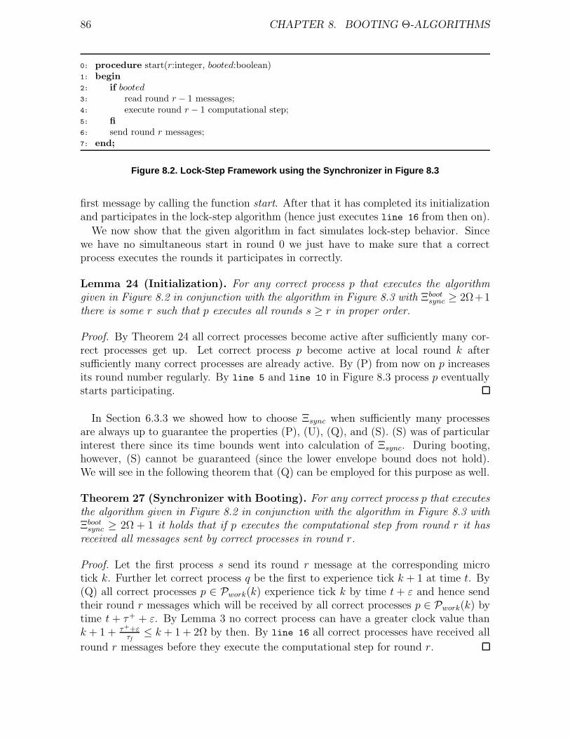
86 CHAPTER 8. BOOTING Θ-ALGORITHMS
0: procedure start(r:integer, booted:boolean)1: begin
2: if booted3: read round r − 1 messages;4: execute round r − 1 computational step;5: fi
6: send round r messages;7: end;
Figure 8.2. Lock-Step Framework using the Synchronizer in Figure 8.3
first message by calling the function start. After that it has completed its initializationand participates in the lock-step algorithm (hence just executes line 16 from then on).
We now show that the given algorithm in fact simulates lock-step behavior. Sincewe have no simultaneous start in round 0 we just have to make sure that a correctprocess executes the rounds it participates in correctly.
Lemma 24 (Initialization). For any correct process p that executes the algorithmgiven in Figure 8.2 in conjunction with the algorithm in Figure 8.3 with Ξboot
sync ≥ 2Ω+1there is some r such that p executes all rounds s ≥ r in proper order.
Proof. By Theorem 24 all correct processes become active after sufficiently many cor-rect processes get up. Let correct process p become active at local round k aftersufficiently many correct processes are already active. By (P) from now on p increasesits round number regularly. By line 5 and line 10 in Figure 8.3 process p eventuallystarts participating.
In Section 6.3.3 we showed how to choose Ξsync when sufficiently many processesare always up to guarantee the properties (P), (U), (Q), and (S). (S) was of particularinterest there since its time bounds went into calculation of Ξsync. During booting,however, (S) cannot be guaranteed (since the lower envelope bound does not hold).We will see in the following theorem that (Q) can be employed for this purpose as well.
Theorem 27 (Synchronizer with Booting). For any correct process p that executesthe algorithm given in Figure 8.2 in conjunction with the algorithm in Figure 8.3 withΞboot
sync ≥ 2Ω + 1 it holds that if p executes the computational step from round r it hasreceived all messages sent by correct processes in round r.
Proof. Let the first process s send its round r message at the corresponding microtick k. Further let correct process q be the first to experience tick k + 1 at time t. By(Q) all correct processes p ∈ Pwork(k) experience tick k by time t + ε and hence sendtheir round r messages which will be received by all correct processes p ∈ Pwork(k) bytime t + τ+ + ε. By Lemma 3 no correct process can have a greater clock value thank + 1 + τ++ε
τf≤ k + 1 + 2Ω by then. By line 16 all correct processes have received all
round r messages before they execute the computational step for round r.
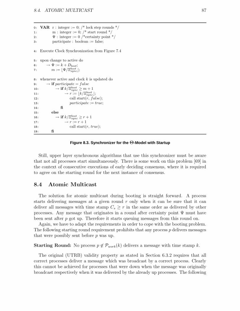
8.4. ATOMIC MULTICAST 87
0: VAR r : integer := 0; /* lock step rounds */1: m : integer := 0; /* start round */2: Ψ : integer := 0 /*certainty point */3: participate : boolean := false;
4: Execute Clock Synchronization from Figure 7.4
5: upon change to active do6: → Ψ := k + Dboot;7: m := bΨ/Ξboot
syncc;
8: whenever active and clock k is updated do9: → if participate = false10: → if k/Ξboot
sync ≥ m + 111: → r := bk/Ξboot
syncc;12: call start(r, false);13: participate := true;14: fi
15: else
16: → if k/Ξbootsync ≥ r + 1
17: → r := r + 118: call start(r, true);19: fi
Figure 8.3. Synchronizer for the Θ-Model with Startup
Still, upper layer synchronous algorithms that use this synchronizer must be awarethat not all processes start simultaneously. There is some work on this problem [69] inthe context of consecutive executions of early deciding consensus, where it is requiredto agree on the starting round for the next instance of consensus.
8.4 Atomic Multicast
The solution for atomic multicast during booting is straight forward. A processstarts delivering messages at a given round r only when it can be sure that it candeliver all messages with time stamp Cs ≥ r in the same order as delivered by otherprocesses. Any message that originates in a round after certainty point Ψ must havebeen sent after p got up. Therefore it starts queuing messages from this round on.
Again, we have to adapt the requirements in order to cope with the booting problem.The following starting round requirement prohibits that any process p delivers messagesthat were possibly sent before p was up.
Starting Round: No process p 6∈ Pwork(k) delivers a message with time stamp k.
The original (UTRB) validity property as stated in Section 6.3.2 requires that allcorrect processes deliver a message which was broadcast by a correct process. Clearlythis cannot be achieved for processes that were down when the message was originallybroadcast respectively when it was delivered by the already up processes. The following
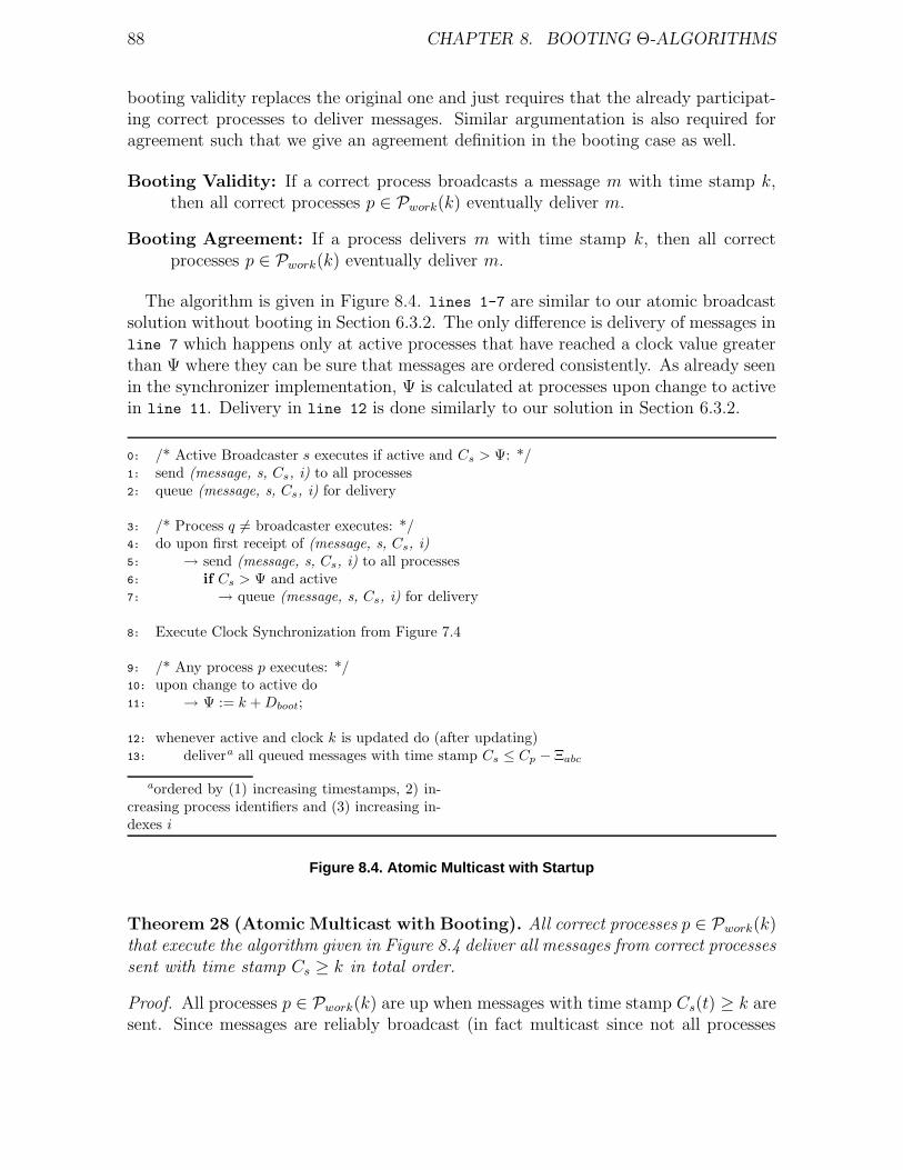
88 CHAPTER 8. BOOTING Θ-ALGORITHMS
booting validity replaces the original one and just requires that the already participat-ing correct processes to deliver messages. Similar argumentation is also required foragreement such that we give an agreement definition in the booting case as well.
Booting Validity: If a correct process broadcasts a message m with time stamp k,then all correct processes p ∈ Pwork(k) eventually deliver m.
Booting Agreement: If a process delivers m with time stamp k, then all correctprocesses p ∈ Pwork(k) eventually deliver m.
The algorithm is given in Figure 8.4. lines 1-7 are similar to our atomic broadcastsolution without booting in Section 6.3.2. The only difference is delivery of messages inline 7 which happens only at active processes that have reached a clock value greaterthan Ψ where they can be sure that messages are ordered consistently. As already seenin the synchronizer implementation, Ψ is calculated at processes upon change to activein line 11. Delivery in line 12 is done similarly to our solution in Section 6.3.2.
0: /* Active Broadcaster s executes if active and Cs > Ψ: */1: send (message, s, Cs, i) to all processes2: queue (message, s, Cs, i) for delivery
3: /* Process q 6= broadcaster executes: */4: do upon first receipt of (message, s, Cs, i)5: → send (message, s, Cs, i) to all processes6: if Cs > Ψ and active7: → queue (message, s, Cs, i) for delivery
8: Execute Clock Synchronization from Figure 7.4
9: /* Any process p executes: */10: upon change to active do11: → Ψ := k + Dboot;
12: whenever active and clock k is updated do (after updating)13: delivera all queued messages with time stamp Cs ≤ Cp − Ξabc
aordered by (1) increasing timestamps, 2) in-creasing process identifiers and (3) increasing in-dexes i
Figure 8.4. Atomic Multicast with Startup
Theorem 28 (Atomic Multicast with Booting). All correct processes p ∈ Pwork(k)that execute the algorithm given in Figure 8.4 deliver all messages from correct processessent with time stamp Cs ≥ k in total order.
Proof. All processes p ∈ Pwork(k) are up when messages with time stamp Cs(t) ≥ k aresent. Since messages are reliably broadcast (in fact multicast since not all processes
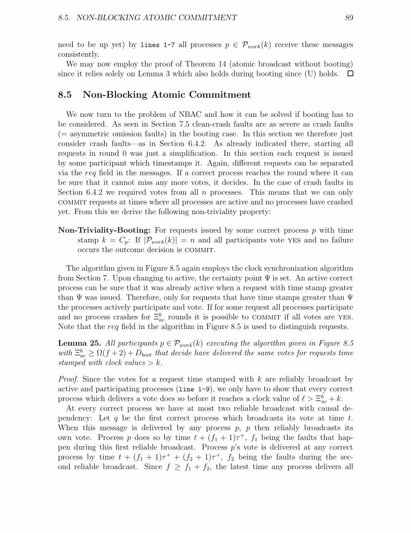
8.5. NON-BLOCKING ATOMIC COMMITMENT 89
need to be up yet) by lines 1-7 all processes p ∈ Pwork(k) receive these messagesconsistently.
We may now employ the proof of Theorem 14 (atomic broadcast without booting)since it relies solely on Lemma 3 which also holds during booting since (U) holds.
8.5 Non-Blocking Atomic Commitment
We now turn to the problem of NBAC and how it can be solved if booting has tobe considered. As seen in Section 7.5 clean-crash faults are as severe as crash faults(= asymmetric omission faults) in the booting case. In this section we therefore justconsider crash faults—as in Section 6.4.2. As already indicated there, starting allrequests in round 0 was just a simplification. In this section each request is issuedby some participant which timestamps it. Again, different requests can be separatedvia the req field in the messages. If a correct process reaches the round where it canbe sure that it cannot miss any more votes, it decides. In the case of crash faults inSection 6.4.2 we required votes from all n processes. This means that we can onlycommit requests at times where all processes are active and no processes have crashedyet. From this we derive the following non-triviality property:
Non-Triviality-Booting: For requests issued by some correct process p with timestamp k = Cp: If |Pwork(k)| = n and all participants vote yes and no failureoccurs the outcome decision is commit.
The algorithm given in Figure 8.5 again employs the clock synchronization algorithmfrom Section 7. Upon changing to active, the certainty point Ψ is set. An active correctprocess can be sure that it was already active when a request with time stamp greaterthan Ψ was issued. Therefore, only for requests that have time stamps greater than Ψthe processes actively participate and vote. If for some request all processes participateand no process crashes for Ξb
ac rounds it is possible to commit if all votes are yes.Note that the req field in the algorithm in Figure 8.5 is used to distinguish requests.
Lemma 25. All participants p ∈ Pwork(k) executing the algorithm given in Figure 8.5with Ξb
ac ≥ Ω(f + 2) + Dboot that decide have delivered the same votes for requests timestamped with clock values > k.
Proof. Since the votes for a request time stamped with k are reliably broadcast byactive and participating processes (line 1-9), we only have to show that every correctprocess which delivers a vote does so before it reaches a clock value of ` > Ξb
ac + k.At every correct process we have at most two reliable broadcast with causal de-
pendency: Let q be the first correct process which broadcasts its vote at time t.When this message is delivered by any process p, p then reliably broadcasts itsown vote. Process p does so by time t + (f1 + 1)τ+, f1 being the faults that hap-pen during this first reliable broadcast. Process p’s vote is delivered at any correctprocess by time t + (f1 + 1)τ+ + (f2 + 1)τ+, f2 being the faults during the sec-ond reliable broadcast. Since f ≥ f1 + f2, the latest time any process delivers all
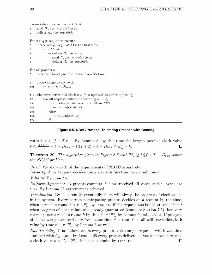
90 CHAPTER 8. BOOTING Θ-ALGORITHMS
To initiate a new request if k ≥ Ψ1: send (k, req, myvote) to all;2: deliver (k, req, myvote);
Process q 6= requester executes:3: if received (l, req, vote) for the first time4: → if l > Ψ5: → deliver (l, req, vote);6: send (l, req, myvote) to all;7: deliver (l, req, myvote);
For all processes8: Execute Clock Synchronization from Section 7
9: upon change to active do10: → Ψ := k + Dboot;
11: whenever active and clock k ≥ Ψ is updated do (after updating)12: For all requests with time stamp ≤ k − Ξb
ac
13: if all votes are delivered and all are yes
14: → return(commit)15: else
16: → return(abort)17: fi
Figure 8.5. NBAC Protocol Tolerating Crashes with Booting
votes is t + (f + 2)τ+. By Lemma 3, by this time the largest possible clock value
` ≤ (f+2)τ+
τf+ k + Dboot = Ω(f + 2) + k + Dboot ≤ Ξb
ac + k.
Theorem 29. The algorithm given in Figure 8.5 with Ξbac ≥ Ω(f + 2) + Dboot solves
the NBAC problem.
Proof. We show each of the requirements of NBAC separately.Integrity: A participant decides using a return function, hence only once.
Validity: By line 15.
Uniform Agreement: A process commits if it has received all votes, and all votes areyes. By Lemma 25 agreement is achieved.
Termination: By Theorem 24 eventually there will always be progress of clock valuesin the system. Every correct participating process decides on a request by the time,when it reaches round ` > k +Ξb
ac by line 14. If the request was issued at some time twhen progress of clock values was already guaranteed (compare Section 7.5) then verycorrect process reaches round k by time t+ τ+Ξb
ac by Lemma 5 and decides. If progressof clocks was guaranteed only from some time t′ > t on, then all will reach this clockvalue by time t′ + τ+Ξb
ac by Lemma 5 as well.
Non-Triviality: If no failure occurs every process votes on p’s request—which was timestamped with Cp—,and by Lemma 25 every process delivers all votes before it reachesa clock value k > Cp + Ξb
ac. It hence commits by line 15.
Chapter 9
Conclusions
9.1 Required Synchrony for Consensus
From a theoretical point of view, when considering new system models one usuallystarts with examining the solvability of consensus in it. Since the presented clocksynchronization algorithms are totally time free (even no a priori knowledge of Θ),they can be employed in several variants of the Θ-Model. We can actually distinguishfour possible system models which have assumptions on Θ:
(1) The variant used in this thesis, i.e. some known Θ that always holds. We haveprovided an implementation of P in this model. This model is hence well suitedfor real-time systems.
(2) We can also think of a model where known Θ holds just from some global stabi-lization time GST on. We have seen that our implementation of P in model (1)can be employed in order to implement P in (2).
(3) Some unknown Θ always holds. In this model P can be implemented as well.Whenever a message from a falsely suspected process p drops in, Ξ must beadapted, according to the current local clock value and the round number of p’smessage. Eventually Ξ will reach the correct value (according to Theorem 9) andour failure detector is perfect from then on.
(4) Some unknown Θ holds from GST on. The same algorithm as in (3) might beemployed but in contrast to model (3), Ξ cannot be guaranteed to be a prioribounded according to Theorem 9 since Θ could be violated before GST. Never-theless we again have an implementation of P.
The previous arguments just refer to crash faults. When considering more severetypes of failures, like Byzantine faults, failure detectors are of no use. For this purposewe provided a simulation which allows to run lock-step algorithms in the Θ-Model inSection 6.3.3. Note also that the consensus algorithms by Dwork, Lynch, and Stock-meyer [37] can easily be transfered into the Θ-Model as well. In [107] we presented asimulation which shows that Byzantine consensus has a solution in a model where theΘ assumptions just holds after some possibly unknown GST.
91
92 CHAPTER 9. CONCLUSIONS
9.2 Clock Synchronization Implementation
When comparing our novel clock synchronization algorithm (see Section 6.1 and Sec-tion 7) to previous ones [106, 109, 67] (which all rely upon the classic non-authenticatedclock synchronization algorithm by Srikanth and Toueg [95]) it is obvious that it is muchsimpler as it requires just one type of messages. Even more important is the propertythat precision (π) and the upper envelope bound of (α) does not depend on τ− butrather upon τf (the round switching time). As already argued in Section 3.5 this eitherleads to improved coverage or improved performance (= smaller values for Θ).
This is particularly important in Ethernet-like networks, where two messages cannotbe sent over the physical link simultaneously. Since messages are sent strictly one afterthe other, one may not need to consider the first message for deriving a bound on Θ.
9.3 Dependable Real-Time Systems
Reviewing this thesis’s results suggests the following approach to build highly reliablesystems: At the basic layer, the clock synchronization with booting (Section 7) shouldbe used. It has the advantage that no a priori knowledge of Θ is required, that it worksunder a wide variety of process and link failures, and that it delivers the synchronyof the communication layer directly to the upper layer. If the system timing hencetemporarily does not behave as assumed, the clock synchronization algorithm keepsworking and just gets out of the assumed bounds. If the system returns to the expectedbehavior the clock synchronization bounds will hold again. This is very important inrecently emerging application domains where it is nearly impossible to predict systembehavior during the whole system operation. Moreover, for such application we haveargued in Section 5.2 that the assumption on the delay ratio is more likely to hold thanassumptions on upper bounds on message delays.
Depending on the types of faults, different layers should be put atop of clock syn-chronization. For crash faults, we propose using the eventually perfect failure detectorP with booting (Section 8.1). Since it has just eventual semantics, every algorithmthat uses P will still satisfy its safety properties even when system timing violationstranslate into false suspicion at the P layer. If the system returns to the expectedbehavior our failure detector becomes perfect again. We can hence guarantee boundeddetection times if our assumptions are met and guarantee safety even if our assump-tions are violated. This property of asynchronous designs is often ignored in real-timeliterature [24] which argues that “compare and kill” is the only solution to ensuresafety. From the distributed computing theory viewpoint Doing nothing is safe! It isof course the task of system engineers to design the interaction with environment insuch a way that the previous statement is true. This results in a more robust, safersolution. We believe that many control problems allow such an approach.
On the other hand keeping systems running although time bounds are violated aslong as the system remains in a consistent state will usually lead to less severe damage.This is especially true in systems where environment conditions are not as predictableas required for many timed solutions (e.g. space borne applications).
9.4. OUTLOOK ON FURTHER RESEARCH DIRECTIONS 93
Atop of the P layer, finally, higher-level algorithms can be devised. Obviouslythere lies a drawback in worst case termination times: Algorithms which use eventualtype failure detectors are usually less effective than those using perpetual ones sincetheir termination times depend on the failure pattern during the execution as well ason the number and pattern of false suspicions. This must taken into account whendimensioning a reliable distributed system.
There is much recent research [36, 35, 58, 13] on failure detector based asynchronousByzantine consensus. To our best knowledge, however, there exists no satisfying def-inition of failure detectors in the case of non-authenticated Byzantine faults by now.We hence propose a different approach to build a system tolerating this kind of faultsin the Θ-Model: Applications may directly be put atop our synchronized clocks, usingthe techniques employed for the solutions of atomic broadcast or non-blocking atomiccommitment (cp. Section 8.4 and Section 8.5; these cannot tolerate Byzantine faults,however). Another approach would be to introduce a synchronization layer that createsthe illusion of lock-step synchrony (Section 8.3) to the applications. It is then possi-ble to run any synchronous algorithm atop of this layer. This easily allows to deviseByzantine-tolerant applications at the cost of possibly higher termination times.
9.4 Outlook on Further Research Directions
The most challenging question in distributed computing theory is the one on theweakest timing model that allows to solve the fundamental, yet not trivial consensusproblem. Therefore it is still subject to currently ongoing work [67, 107, 41, 2, 76].Although the Θ-Model provides an important step towards this goal, there is stillroom for improvement. For example, just reconciling some of the mentioned approachesmight lead to even weaker timing models.
In the case of the Θ-Model, we mentioned in Section 3.4 that the length ratio of twoconcurrent message chains is bounded by Θ as consequence of our system model (cp.Section 3.2). Bounding just these length ratio instead of bounding message end-to-enddelays might lead to an even weaker system model that allows to solve consensus. Oneimportant point, however, must always be regarded: Can the envisioned system modelbe implemented in real systems? We showed in Section 5.5 that the Θ-Model can infact be implemented very efficiently in real-time systems. Other approaches [24, 76]that try to weaken the system model, however, just provide probabilistic guarantees.We believe that it is mandatory to show how to implement the new models in order toremain in contact with real systems and real problems.
An issue which is closely related to the timing of distributed systems is queuing. Itwould be an interesting topic for future research whether we can give analytical feasi-bility conditions for systems that guarantee applicability of the Θ-Model. As a startingpoint for such research some networks of queues—as depicted in Figure 2.1—must beanalyzed. This analysis, however, must not rely on time triggered processes—as oftenassumed in queuing theory—but on event based ones and must consider adversariesaccording to the particular failure model used.

94 CHAPTER 9. CONCLUSIONS
Apart from timing models, there are also open questions on fault models. The self-stabilization [28, 31] paradigm, for example, does not model permanent, but rather arbi-trary transient faults. A very interesting research field are fault-tolerant self-stabilizing(ftss) algorithms. Reconciling ftss and time free algorithms leads to even more reliablesystems. For the Θ-Model, we have presented ftss failure detector implementations [55].But many more problems are out there that must be solved.
An interesting research field lies between classic fault-tolerance and ftss. The crashrecovery model [3] describes transient faults which do not lead to an arbitrary systemstate, as assumed in self-stabilization. For the Θ-Model we have solved the bootingproblem, for example. It seems as if this might be half the way to crash recovery:For example, one might think of a similar non-blocking atomic commit algorithm asthe one in Section 8.5 that may be employed in the crash recovery model. We wouldrequire that at least f + 1 processes do not crash after they have booted. The othersmay crash and recover. A decision commit can be reached during periods when allprocesses are active.
Bibliography
[1] Marcos Aguilera, Gerard Le Lann, and Sam Toueg. On the impact of fast failuredetectors on real-time fault-tolerant systems. In Proceedings of the 16th Interna-tional Symposium on Distributed Computing (DISC’02), volume 2508 of LNCS,pages 354–369. Springer Verlag, Oct 2002.
[2] Marcos K. Aguilera, Carole Delporte-Gallet, Hugues Fauconnier, and Sam Toueg.On implementing Omega with weak reliability and synchrony assumptions. InProceeding of the 22nd Annual ACM Symposium on Principles of DistributedComputing (PODC’03), 2003.
[3] Marcos Kawazoe Aguilera, Wei Chen, and Sam Toueg. Failure detection andconsensus in the crash-recovery model. Distributed Computing, 13(2):99–125,April 2000.
[4] Marcos Kawazoe Aguilera, Wei Chen, and Sam Toueg. On quiescent reliablecommunication. SIAM Journal of Computing, 29(6):2040–2073, April 2000.
[5] Daniel Albeseder. Experimentelle Verifikation von Synchronitatsannahmen furComputernetzwerke. Diplomarbeit, Embedded Computing Systems Group, Tech-nische Universitat Wien, May 2004.
[6] Anish Arora, Shlomi Dolev, and Mohamed G. Gouda. Maintaining digital clocksin step. In Sam Toueg, Paul G. Spirakis, and Lefteris M. Kirousis, editors,Distributed Algorithms, 5th International Workshop, volume 579, pages 71–79,Delphi, Greece, 7–9 1991. Springer-Verlag.
[7] Hagit Attiya, Danny Dolev, and Joseph Gil. Asynchronous byzantine consensus.Proceedings of the 3rd ACM Symposium of Distributed Computing, pages 119–133, August 1984.
[8] Hagit Attiya, Cynthia Dwork, Nancy Lynch, and Larry Stockmeyer. Bounds onthe time to reach agreement in the presence of timing uncertainty. Journal of theACM (JACM), 41(1):122–152, 1994.
[9] Hagit Attiya and Jennifer Welch. Distributed Computing. McGraw-Hill, 1998.
[10] Baruch Awerbuch. Complexity of network synchronization. Journal of the ACM(JACM), 32(4):804–823, 1985.
95
96 BIBLIOGRAPHY
[11] M.H. Azadmanesh and Roger M. Kieckhafer. Exploiting omissive faultsin synchronous approximate agreement. IEEE Transactions on Computers,49(10):1031–1042, October 2000.
[12] Ozalp Babaoglu and Sam Toueg. Non-blocking atomic commitment. In SapeMullender, editor, Distributed Systems 2nd Ed., pages 147–166. ACM Press, 1993.
[13] Roberto Baldoni, Jean-Michel Helary, Michel Raynal, and Lenaik Tangui. Con-sensus in byzantine asynchronous systems. Journal of Discrete Algorithms,1(2):185–210, 2003.
[14] Boaz Barak, Shai Halevi, Amir Herzberg, and Dalit Naor. Clock synchronizationwith faults and recoveries (extended abstract). In Proceedings of the nineteenthannual ACM symposium on Principles of distributed computing, pages 133–142.ACM Press, 2000.
[15] Marin Bertier, Olivier Marin, and Pierre Sens. Implementation and perfor-mance evaluation of an adaptable failure detector. In Proceedings of the In-ternational Conference on Dependable Systems and Networks (DSN’02), pages354–363, Washington, DC, June 23–26, 2002.
[16] Martin Biely. An optimal Byzantine agreement algorithm with arbitrary nodeand link failures. In Proc. 15th Annual IASTED International Conference onParallel and Distributed Computing and Systems (PDCS’03), pages 146–151, Ma-rina Del Rey, California, USA, November 3–5, 2003.
[17] A. Casimiro, P. Martins, and P. Verıssimo. How to build a timely computing baseusing real-time linux. In Proceedings of the 2000 IEEE International Workshopon Factory Communication Systems, pages 127–134, Porto, Portugal, September2000. IEEE Industrial Electronics Society.
[18] Tushar Deepak Chandra, Vassos Hadzilacos, and Sam Toueg. The weakest failuredetector for solving consensus. Journal of the ACM, 43(4):685–722, June 1996.
[19] Tushar Deepak Chandra and Sam Toueg. Unreliable failure detectors for reliabledistributed systems. Journal of the ACM, 43(2):225–267, March 1996.
[20] Bernadette Charron-Bost. Comparing the atomic commitment and consensusproblems. In Future Directions in Distributed Computing 2002, volume 2584 ofLNCS, pages 29–34. Springer-Verlag, 2003.
[21] Bernadette Charron-Bost, Rachid Guerraoui, and Andre Schiper. Synchronoussystem and perfect failure detector: Solvability and efficiency issues. In Pro-ceedings of the IEEE Int. Conf. on Dependable Systems and Networks (DSN’00),pages 523–532, New York, USA, 2000. IEEE Computer Society.

BIBLIOGRAPHY 97
[22] Wei Chen, Sam Toueg, and Marcos Kawazoe Aguilera. On the quality of serviceof failure detectors. In Proceedings IEEE International Conference on DependableSystems and Networks (ICDSN / FTCS’30), 2000.
[23] George Coulouris, Jean Dollimore, and Tim Kindberg. Distributed Systems. As-sison Wesley, 3rd edition, 2000.
[24] Flaviu Cristian and Christof Fetzer. The timed asynchronous distributed systemmodel. IEEE Transactions on Parallel and Distributed Systems, 10(6):642–657,1999.
[25] Ariel Daliot, Danny Dolev, and Hanna Parnas. Linear time byzantine self-stabilizing clock synchronization. In Proceedings of the 7th International Confer-ence on Principles of Distributed Systems, Dec 2003. to appear.
[26] Ariel Daliot, Danny Dolev, and Hanna Parnas. Self-stabilizing pulse synchro-nization inspired by biological pacemaker networks. In Proceedings of the 6thInternational Symposium on Self-Stabilizing Systems, SSS’03, volume 2704 ofLNCS, pages 32–48. Springer Verlag, June 2003.
[27] Susan B. Davidson, Insup Lee, and Victor Wolfe. Timed atomic commitment.In IEEE Transactions on Computers, volume 40, pages 573–583, May 1991.
[28] Edsger W. Dijkstra. Self-stabilizing systems in spite of distributed control. Com-munications of the ACM, 17(11):643–644, 1974.
[29] Danny Dolev, Cynthia Dwork, and Larry Stockmeyer. On the minimal synchro-nism needed for distributed consensus. Journal of the ACM, 34(1):77–97, January1987.
[30] Danny Dolev, Joseph Y. Halpern, and H. Raymond Strong. On the possibilityand impossibility of achieving clock synchronization. Journal of Computer andSystem Sciences, 32:230–250, 1986.
[31] Shlomi Dolev. Self-Stabilization. MIT Press, 2000.
[32] Shlomi Dolev and Jennifer L. Welch. Wait-free clock synchronization. In Proceed-ing of the 12th Annual ACM Symposium on Principles of Distributed Computing(PODC’93), pages 97–108, 1993.
[33] Shlomi Dolev and Jennifer L. Welch. Self-stabilizing clock synchronization in thepresence of byzantine faults. In Proc. of the 2nd Workshop on Self-StabilizingSystems, May 1995.
[34] Shlomi Dolev and Jennifer L. Welch. Wait-free clock synchronization. Algorith-mica, 18(4):486–511, 1997.
98 BIBLIOGRAPHY
[35] Assia Doudou, Benoit Garbinato, Rachid Guerraoui, and Andre Schiper. Mute-ness failure detectors: Specification and implementation. In Proceedings 3rdEuropean Dependable Computing Conference (EDCC-3), volume 1667 of LNCS1667, pages 71–87. Springer, September 1999.
[36] Assia Doudou and Andre Schiper. Muteness detectors for consensus with byzan-tine processes. In Proceedings of the 17th ACM Symposium on Principles ofDistributed Computing (PODC-17), 1998.
[37] Cynthia Dwork, Nancy Lynch, and Larry Stockmeyer. Consensus in the presenceof partial synchrony. Journal of the ACM, 35(2):288–323, April 1988.
[38] Cynthia Dwork and Dale Skeen. The inherent cost of nonblocking commitment.In Proceedings of the second annual ACM symposium on Principles of distributedcomputing, pages 1–11. ACM Press, 1983.
[39] R. Ernst and W. Ye. Embedded program timing analysis based on path cluster-ing and architecture classification. In Digest of Technical Papers of IEEE/ACMInternational Conference on Computer-Aided Design, pages 598–604. IEEE Com-puter Society, April 1997.
[40] Christof Fetzer, Michel Raynal, and Frederic Tronel. An adaptive failure detec-tion protocol. In Pacific Rim International Symposium on Dependable Computing(PRDC 2001), December 2001.
[41] Christof Fetzer and Ulrich Schmid. On the possibility of consensus in asyn-chronous systems with finite average response times. Research Report 14/2004,Technische Universitat Wien, Institut fur Technische Informatik, Treitlstraße 3,A-1040 Vienna, Austria, 2004. (submitted).
[42] Michael J. Fischer, Nancy A. Lynch, and M. S. Paterson. Impossibility of dis-tributed consensus with one faulty processor. Journal of the ACM, 32(2):374–382,April 1985.
[43] Eli Gafni. Round-by-round fault detectors (extended abstract): unifying syn-chrony and asynchrony. In Proceedings of the Seventeenth Annual ACM Sympo-sium on Principles of Distributed Computing, pages 143–152. ACM Press, 1998.
[44] Vijay K. Garg and J. Roger Mitchell. Implementable failure detectors in asyn-chronous systems. In Proceedings of the 18th Int. Conference on Foundations ofSoftware Technology and Theoretical Computer Science (FST & TCS’98), LNCS1530, pages 158–169. Springer, 1998.
[45] Jim N. Gray. Notes on data base operating systems. In G. Seegmuller R. Bayer,R.M. Graham, editor, Operating Systems: An Advanced Course, volume 60 ofLecture Notes in Computer Science, chapter 3.F, page 465. Springer, New York,1978.
BIBLIOGRAPHY 99
[46] R. Guerraoui and A. Schiper. The decentralized non-blocking atomic commit-ment protocol. In Proceedings of the 7th IEEE Symposium on Parallel and Dis-tributed Processing (SPDP-7), pages 2–9, San Antonio, Texas, USA, 1995.
[47] Rachid Guerraoui. Non-blocking atomic commit in asynchronous distributedsystems with failure detectors. Distributed Computing, 15:17–25, 2002.
[48] Indranil Gupta, Tushar D. Chandra, and German S. Goldszmidt. On scalable andefficient distributed failure detectors. In Proceedings of the 20th ACM Symposiumon Principles of Distributed Computing (PODC’01), pages 170–179, August 2001.
[49] J.C. Palencia Gutierrez, J.J. Gutierrez Garcia, and M. Gonzales Harbour. Best-case analysis for improving the worst-case schedulability test for distributed hardreal-time systems. In Proceedings of the 10th Euromicro Workshop on Real-TimeSystems, pages 35–44, June 1998.
[50] Vassos Hadzilacos and Sam Toueg. Fault-tolerant broadcasts and related prob-lems. In Sape Mullender, editor, Distributed Systems, chapter 5, pages 97–145.Addison-Wesley, 2nd edition, 1993.
[51] J.-F. Hermant and Gerard Le Lann. Fast asynchronous uniform consensus inreal-time distributed systems. IEEE Transactions on Computers, 51(8):931–944,August 2002.
[52] J.-F. Hermant and Josef Widder. Implementing time free designs for distributedreal-time systems (a case study). Research Report 23/2004, Technische Univer-sitat Wien, Institut fur Technische Informatik, May 2004. Joint Research Reportwith INRIA Rocquencourt. (submitted for publication).
[53] M. Hurfin and M. Raynal. Asynchronous protocols to meet real-time constraints:Is it really feasible? How to proceed? In Proceedings of the IEEE Intl. Symposiumon Object-Oriented Real-Time Distributed Computing (ISORC), pages 290–297.IEEE Computer Society, April 2003.
[54] Martin Hutle. An efficient failure detector for sparsely connected networks. InProc. IASTED International Conference on Parallel and Distributed Computingand Networks (PDCN’04), Innsbruck, Austria, February 2004.
[55] Martin Hutle and Josef Widder. Time free self-stabilizing local failure detection,May 2004. (submitted for publication).
[56] E.D. Jensen and B Ravindran. Guest editors’ introduction to special section onasynchronous real-time distributed systems. IEEE Transactions on Computers,51(8):881–882, August 2002.
[57] Roger M. Kieckhafer, Chris J. Walter, Alan M. Finn, and Philip M. Thambidurai.The MAFT architecture for distributed fault tolerance. IEEE Transactions onComputers, 37:398–405, April 1988.
100 BIBLIOGRAPHY
[58] Kim Potter Kihlstrom, Louise E. Moser, and P. M. Melliar-Smith. Byzantinefault detectors for solving consensus. The Computer Journal, 46(1):16–35, 2003.
[59] Hermann Kopetz. Real-Time Systems. Design Principles for Distributed Embed-ded Applications. Kluwer Academic Publishers, 1997.
[60] Leslie Lamport, Robert Shostak, and Marshall Pease. The Byzantine generalsproblem. ACM Transactions on Programming Languages and Systems, 4(3):382–401, July 1982.
[61] Mikel Larrea, Antonio Fernandez, and Sergio Arevalo. Efficient algorithms to im-plement unreliable failure detectors in partially synchronous systems. In Proceed-ings of the 13th International Symposium on Distributed Computing (DISC’99),LNCS 1693, pages 34–48. Springer, September 1999.
[62] Mikel Larrea, Antonio Fernandez, and Sergio Arevalo. Optimal implementationof the weakest failure detector for sloving consensus. In Proceedings of the 19thACM Symposium on Principles of Distributed Computing (PODC’00), page 334,2000.
[63] Mikel Larrea, Antonio Fernandez, and Sergio Arevalo. On the impossibility of im-plementing perpetual failure detectors in partially synchronous systems. In Pro-ceedings of the 10th Euromicro Workshop on Parallel, Distributed and Network-based Processing (PDP’02), January 2002.
[64] Gerard Le Lann. Certifiable critical complex computing systems. In K. Duncanand K. Krueger, editors, Proceedings 13th IFIP World Computer Congress 94,volume 3, pages 287–294. Elsevier Science B.V. (North-Holland), 1994.
[65] Gerard Le Lann. On real-time and non real-time distributed computing. In Pro-ceedings 9th International Workshop on Distributed Algorithms (WDAG’95), vol-ume 972 of Lecture Notes in Computer Science, pages 51–70. Springer, September1995.
[66] Gerard Le Lann. Asynchrony and real-time dependable computing. In Proceed-ings of the 8th IEEE Intl. Workshop on Object-Oriented Real-Time DependableSystems (WORDS 2003), page 8p., Guadalajara, Mexico, 2003. IEEE ComputerSociety.
[67] Gerard Le Lann and Ulrich Schmid. How to implement a timer-free perfect failuredetector in partially synchronous systems. Technical Report 183/1-127, Depart-ment of Automation, Technische Universitat Wien, January 2003. (submitted).
[68] Gerard Le Lann and Ulrich Schmid. How to maximize computing systems cov-erage. Technical Report 183/1-128, Department of Automation, Technische Uni-versitat Wien, April 2003.
BIBLIOGRAPHY 101
[69] Yehuda Lindell, Anna Lysyanskaya, and Tal Rabin. Sequential composition ofprotocols without simultaneous termination. In Proceedings of the twenty-firstannual symposium on Principles of distributed computing, pages 203–212. ACMPress, 2002.
[70] Jennifer Lundelius-Welch and Nancy A. Lynch. A new fault-tolerant algorithmfor clock synchronization. Information and Computation, 77(1):1–36, 1988.
[71] Nancy Lynch. Distributed Algorithms. Morgan Kaufman, 1996.
[72] Stephen R. Mahaney and Fred B. Schneider. Inexact agreement: Accuracy,precision, and graceful degradation. In Proceedings 4th ACM Symposium onPrinciples of Distributed Computing, pages 237–249, Minaki, Canada, August1985.
[73] Paul S. Miner. Verification of fault-tolerant clock synchronization systems. NASATechnical Paper 3349, November 1993.
[74] Shivakant Mishra and Cristof Fetzer. The timewheel group communication sys-tem. IEEE Transactions on Computers, 51(8):883–899, August 2002.
[75] Achour Mostefaoui, David Powell, and Michel Raynal. A hybrid approach forbuilding eventually accurate failure detectors. In Proceedings of the 10th IEEEPacific Rim International Symposium on Dependable Computing (PRDC 2004),3-5 March 2004, Papeete, Tahiti, pages 57–65. IEEE Computer Society, 2004.
[76] Anchour Mostefaoui, Eric Mourgaya, and Michel Raynal. Asynchronous imple-mentation of failure detectors. In Proceedings of the International Conference onDependable Systems and Networks (DSN’03), San Francisco, CA, June 22–25,2003.
[77] Sape Mullender. Distributed Systems. ACM Press/Addison Wesley, New York,2nd ed. edition, 1993.
[78] Marina Papatriantafilou and Philippas Tsigas. Self-stabilizing wait-free clocksynchronization. Technical Report CS-R9421, Centrum voor Wiskunde and In-formatica, Netherlands, 1994.
[79] Marina Papatriantafilou and Philippas Tsigas. On self-stabilizing wait-free clocksynchronization. Parallel Processing Letters, 7(3):321–328, 1997.
[80] S. Ponzio. The real-time cost of timing uncertainty: Consensus and failure de-tection. Master’s thesis, Massachusetts Institute of Technology, May 1991.
[81] Stephen Ponzio and Ray Strong. Semisynchrony and real time. In Proceedingsof the 6th International Workshop on Distributed Algorithms (WDAG’92), pages120–135, November 1992.
102 BIBLIOGRAPHY
[82] Parameswaran Ramanathan, Kang G. Shin, and Ricky W. Butler. Fault-tolerantclock synchronization in distributed systems. IEEE Computer, 23(10):33–42,October 1990.
[83] Michel Raynal. A case study of agreement problems in distributed systems:non-blocking atomic commitment. In Proceedings of High-Assurance SystemsEngineering Workshop, pages 209–214, Aug 1997.
[84] Ulrich Schmid, editor. Special Issue on The Challenge of Global Time in Large-Scale Distributed Real-Time Systems, Real-Time Systems 12(1–3), 1997.
[85] Ulrich Schmid. Orthogonal accuracy clock synchronization. Chicago Journal ofTheoretical Computer Science, 2000(3):3–77, 2000.
[86] Ulrich Schmid. How to model link failures: A perception-based fault model. InProceedings of the International Conference on Dependable Systems and Networks(DSN’01), pages 57–66, Goteborg, Sweden, July 1–4, 2001.
[87] Ulrich Schmid and Christof Fetzer. Randomized asynchronous consensus withimperfect communications. Technical Report 183/1-120, Department of Automa-tion, Technische Universitat Wien, January 2002. (Extended version of [88]).
[88] Ulrich Schmid and Christof Fetzer. Randomized asynchronous consensus withimperfect communications. In 22nd Symposium on Reliable Distributed Systems(SRDS’03), pages 361–370, October 6–8, 2003.
[89] Ulrich Schmid and Klaus Schossmaier. Interval-based clock synchronization.Real-Time Systems, 12(2):173–228, March 1997.
[90] Ulrich Schmid and Bettina Weiss. Synchronous Byzantine agreement under hy-brid process and link failures. Technical Report 183/1-124, Department of Au-tomation, Technische Universitat Wien, November 2002. (replaces TR 183/1-110).
[91] Ulrich Schmid, Bettina Weiss, and John Rushby. Formally verified byzantineagreement in presence of link faults. In 22nd International Conference on Dis-tributed Computing Systems (ICDCS’02), pages 608–616, July 2-5, 2002.
[92] Fred B. Schneider. Understanding protocols for byzantine clock synchronization.Technical Report 87-859, Cornell University, Department of Computer Science,August 1987.
[93] Barbara Simons, Jennifer Lundelius-Welch, and Nancy Lynch. An overview ofclock synchronization. In Barbara Simons and A. Spector, editors, Fault-TolerantDistributed Computing, pages 84–96. Springer Verlag, 1990. (Lecture Notes onComputer Science 448).
BIBLIOGRAPHY 103
[94] Paul Spirakis and Basil Tampakas. Efficient distributed algorithms by usingthe archimedean time assumption. In Proceedings of the 5th Annual Symposiumon Theoretical Aspects of Computer Science (STACS 88), volume 294 of LNCS,pages 248–263. Springer Verlag, February 1988.
[95] T. K. Srikanth and Sam Toueg. Optimal clock synchronization. Journal of theACM, 34(3):626–645, July 1987.
[96] Wilfried Steiner and Michael Paulitsch. The transition from asynchronous to syn-chronous system operation: An approach for distributed fault-tolerant systems.Proceedings of the The 22nd International Conference on Distributed ComputingSystems, July 2002.
[97] Andrew S. Tanenbaum and Maarten van Steen. Distributed Systems. Principlesand Paradigms. Prentice Hall, 2001.
[98] Gerard Tel. Introduction to Distributed Algorithms. Cambridge University Press,2001.
[99] Paulo Verıssimo and Antonio Casimiro. The timely computing base model andarchitecture. IEEE Transactions on Computers, 51(8):916–930, August 2002.
[100] Paulo Verıssimo, Antonio Casimiro, and Christof Fetzer. The timely computingbase: Timely actions in the presence of uncertain timeliness. In ProceedingsIEEE International Conference on Dependable Systems and Networks (DSN’01/ FTCS’30), pages 533–542, 2000.
[101] Paulo Verıssimo and Luıs Rodrigues. Distributed Systems for System Architects.Kluwer Academic Publishers, 2001.
[102] Paul M.B. Vitanyi. Distributed elections in an archimedean ring of processors.In Proceedings of the sixteenth annual ACM symposium on Theory of computing,pages 542–547. ACM Press, 1984.
[103] Paul M.B. Vitanyi. Time-driven algorithms for distributed control. Report CS-R8510, C.W.I., May 1985.
[104] Chris J. Walter and Neeraj Suri. The customizable fault/error model for depend-able distributed systems. Theoretical Computer Science, 290:1223–1251, October2002.
[105] Bettina Weiss and Ulrich Schmid. Consensus with written messages under linkfaults. In 20th Symposium on Reliable Distributed Systems (SRDS’01), pages194–197, October 28–31, 2001.
[106] Josef Widder. Booting clock synchronization in partially synchronous systems.In Proceedings of the 17th International Symposium on Distributed Computing(DISC’03), volume 2848 of LNCS, pages 121–135. Springer Verlag, October 2003.
104 BIBLIOGRAPHY
[107] Josef Widder. Consensus in the presence of bounded asynchrony: A simulation(extended abstract), May 2004. (submitted for publication).
[108] Josef Widder, Gerard Le Lann, and Ulrich Schmid. Perfect failure detectionwith booting in partially synchronous systems. Technical Report 183/1-131,Department of Automation, Technische Universitat Wien, April 2003.
[109] Josef Widder and Ulrich Schmid. Booting clock synchronization in partiallysynchronous systems with hybrid node and link failures. Technical Report 183/1-126, Department of Automation, Technische Universitat Wien, January 2003.(submitted for publication).

Curriculum Vitae
Josef Widder
1110 Vienna, Meidlgasse 41/4/4
Personal DataDate of Birth: March, 18, 1977Place of Birth: ViennaCitizenship: Austria
Education1983 – 1987 Volksschule (elementary school)
1110 Wien, Hoefftgasse 71987 – 1991 Bundesrealgymnasium (grammar school)
2320 Schwechat, Ehrenbrunngasse 61991 – 1996 Hohere Technische Bundeslehranstalt
Abteilung fur EDV/Betriebstechnik(polytechnic - EDP/engineering department)1030 Wien, Ungargasse 69
1996 – 2002 Technische Universitat Wien – Informatik(Vienna University of Technology – Computer Science)academic degree: Diplomingenieur (Master of Science)
Working ExperienceJuly 1993 and July 1995 summer job at Fa. Zorkler
gearwheel technologies & mechanical engineeringJuly – August 1997 summer job at SpardatSept 1997 – Jan 1998 working student at Spardat: Software developerSeptember 2000 Die Donau - Danube Tourist Commission
Homepage development danube-river.org(Special Award of the Jury was given by themagazine ”tourist austria” in June 2001)
May 2001–May 2002 volunteer: Aktion Leben Osterreichdevelopment of donator/donations database
Jan 2003 – present research assistant at TU ViennaAutomation Systems Group andEmbedded Computing Systems Group