Solving LFP by Converting it into a Single LP - ORSTW No. 3, pp.1-14.pdf · Solving LFP by...
14
International Journal of Operations Research Vol.8, No. 3, 1-14 (2011) Solving LFP by Converting it into a Single LP Mohammad Babul Hasan 1* and Sumi Acharjee 2, ψ 1,2 Department of Mathematics, University of Dhaka, Dhaka-1000, Bangladesh. Received December 2010; Revised May 2011; Accepted June 2011 Abstract - In this paper, we introduce a computer-oriented technique for solving Linear Fractional Programming (LFP) problem by converting it into a single Linear programming (LP) problem. We develop this computer technique using programming language MATHEMATICA. We illustrate a number of numerical examples to demonstrate our method. We then compare our method with other existing methods in the literature for solving LFP problems. Keywords LP, LFP, Computer technique, Mathematica. 1. INTRODUCTION Linear fractional programming (LFP) deals with that class of mathematical programming problems in which the relations among the variables are linear: the constraint relations must be in linear form and the objective function to be optimized must be a ratio of two linear functions. This field of LFP was developed by Hungarian mathematician B. Matros in 1960 (1960, 1964). Nowadays linear fractional criterion is frequently encountered in business and economics such as: Min [debt-to-equity ratio], Max [return on investment], Min [Risk asset to Capital], Max [Actual capital to required capital] etc. So, the importance of LFP problems is evident. There are a number of methods for solving the LFP problems. Among them the transformation technique developed by Charnes and Cooper (1962, 1973), the simplex type algorithm introduced by Swarup (1964, 2003) and Bitran & Novae’s method (1972) are widely accepted. Tantawy (2007) developed a technique with the dual solution. But from the analysis of these methods, we observe that these methods are lengthy, time consuming and clumsy. In this paper, we will develop a technique for solving LFP problem by converting it into a single linear programming (LP) problem. This method makes the LFP so easy that, we can solve any kind of LFP problem by using this method. Later, we develop a computer technique to implement this method by using programming language MATHEMATICA (2000, 2001) for solving LFP problems. We also make a comparison between our method and other well-known methods for solving LFP problems. 1.1. Relation between LP and LFP In this section, we establish the relationship between LP and LFP problems. The mathematical form of an LP is as follows: Maximize (Minimize) Z cx = (1) subject to Ax b = (2) * Corresponding author’s email: [email protected] ψ Email: [email protected] International Journal of Operations Research
Transcript of Solving LFP by Converting it into a Single LP - ORSTW No. 3, pp.1-14.pdf · Solving LFP by...
International Journal of Operations Research Vol.8, No. 3, 1-14 (2011)
Solving LFP by Converting it into a Single LP
Mohammad Babul Hasan1* and Sumi Acharjee2,ψ
1,2Department of Mathematics, University of Dhaka, Dhaka-1000, Bangladesh.
Received December 2010; Revised May 2011; Accepted June 2011
Abstract - In this paper, we introduce a computer-oriented technique for solving Linear Fractional Programming (LFP) problem by converting it into a single Linear programming (LP) problem. We develop this computer technique using programming language MATHEMATICA. We illustrate a number of numerical examples to demonstrate our method. We then compare our method with other existing methods in the literature for solving LFP problems. Keywords LP, LFP, Computer technique, Mathematica.
1. INTRODUCTION
Linear fractional programming (LFP) deals with that class of mathematical programming problems in which the relations among the variables are linear: the constraint relations must be in linear form and the objective function to be optimized must be a ratio of two linear functions. This field of LFP was developed by Hungarian mathematician B. Matros in 1960 (1960, 1964). Nowadays linear fractional criterion is frequently encountered in business and economics such as: Min [debt-to-equity ratio], Max [return on investment], Min [Risk asset to Capital], Max [Actual capital to required capital] etc. So, the importance of LFP problems is evident. There are a number of methods for solving the LFP problems. Among them the transformation technique developed by Charnes and Cooper (1962, 1973), the simplex type algorithm introduced by Swarup (1964, 2003) and Bitran & Novae’s method (1972) are widely accepted. Tantawy (2007) developed a technique with the dual solution. But from the analysis of these methods, we observe that these methods are lengthy, time consuming and clumsy. In this paper, we will develop a technique for solving LFP problem by converting it into a single linear programming (LP) problem. This method makes the LFP so easy that, we can solve any kind of LFP problem by using this method. Later, we develop a computer technique to implement this method by using programming language MATHEMATICA (2000, 2001) for solving LFP problems. We also make a comparison between our method and other well-known methods for solving LFP problems.
1.1. Relation between LP and LFP
In this section, we establish the relationship between LP and LFP problems. The mathematical form of an LP is as follows:
Maximize (Minimize) Z cx= (1)
subject to Ax b= (2)
* Corresponding author’s email: [email protected] ψ Email: [email protected]
International Journal of Operations Research
2 Babul Hasan and Sumi Acharjee: Solving LFP by Converting it into a Single LP IJOR Vol. 8, No. 3, 1-14 (2011)
0x ≥ (3)
0b ≥ (4)
where, ( )1 2 1, , , , ,m m na a a aA a+…… …= is a m n× matrix, mb R∈ , , nx c R∈ , x is a ( )1n× column vector, and c is a
( )1 n× row vector.
And the mathematical formulation of an LFP is as follows:
Maximize Z cxdx
αβ
+=
+ (5)
subject to Ax b≤ (6)
0x ≥ (7)
where, ( )1 2 1, , , , ,m m na a a aA a+…… …= is a m n× matrix, mb R∈ , , , nx c d R∈ , , Rα β ∈ .
It is assumed that the feasible region { }: , 0n Ax bS x xR∈ ≤ ≥= is nonempty and bounded and the denominator
0dx β+ ≠ .
Now, If 0d = and 1β = then the LFP in (5) to (7) becomes an LP problem. That is (5) can be written as:
Maximize Z cx α= + subject to Ax b≤ ; 0x ≥ .
This is why we say that LFP is a generalization of an LP in (1) to (3). There are also a few cases when the LFP can be replaced with an appropriate LP. These cases are discussed as follows:
Case 1:
If 0d = and 1β ≠ in (5), then Z becomes a linear function
1
Z c Zx αβ β β
+ == , where 1Z cx α= + is a linear function.
In this case Z may be substituted with 1
Zβ
corresponding to the same set of feasible region S. As a result the LFP
becomes an LP.
Case 2:
If 0c = in (5) then 2 dx Z
Z α αβ=
+= , where 2Z dx β= + is a linear function.
In this case, Z becomes linear on the same set of feasible solution S. Therefore the LFP results in an LP with the same feasible region S.
Case 3:
If 1 2( , , )nc cc c ……………= , 1 2( , , )nd dd d ……………= are linearly dependent, there exists 0µ ≠ such that c dµ= ,
then dxdx dx
Z µ α α µβµβ β+ −
= +=+ +
Z
(i) if 0α µβ− = , then Z µ= is a constant.
3 Babul Hasan and Sumi Acharjee: Solving LFP by Converting it into a Single LP IJOR Vol. 8, No. 3, 1-14 (2011)
(ii)if 0α µβ− > or 0α µβ− < i.e., if 0α µβ− ≠ then Z becomes a linear function. Therefore the LFP becomes an LP with the same feasible region S.
If 0c ≠ and 0d ≠ then one has to find a new way to convert the LFP into an LP. Assuming that the feasible region
{ }: , 0nS x R Ax b x= ∈ ≤ ≥
is nonempty and bounded and the denominator 0dx β+ > , we develop a method which converts an LFP of this type to an LP.
The rest of the paper is organized as follows. In Section 2, we discuss the well-known existing methods such as Charnes & Coopers method (1962), Bitran & Novaes method (1972) and Swarup’s method (1964). In Section 3, we discuss our method. Here we also develop a computer technique for this method by using programming language MATHEMATICA. We illustrate the solution procedure with a number of numerical examples. In Section 4, we make a comparison between our method and other well-known methods considered in this research. Finally, we draw a conclusion in Section 5. 2. EXISTING METHODS In this section, we briefly discuss most relevant existing research articles for solving LFP problems. 2.1 Charnes and Coopers method (1962) Charnes-Cooper (1962) considered the LFP problem defined by (5), (6) and (7) on the basis of the assumptions:
i. The feasible region X is nonempty and bounded. ii. cx α+ and dx β+ do not vanish simultaneously in S.
The authors then used the variable transformation y tx= , 0t ≥ , in such a way that dt β γ+ = where 0γ ≠ is a specified number and transform LFP to an LP problem. Multiplying numerator and denominator and the system of inequalities (6) by t and taking y tx= , 0t ≥ into account, they obtain two equivalent LP problems and named them as EP and EN as follows:
(EP) Maximize ( ), L y t cy tα≡ +
subject to, 0Ay bt− ≤ , dy tβ γ+ = , , 0y t ≥ And (EN) Maximize -cy- tα subject to, 0Ay bt− ≤ , 1dy tβ− − = , , 0y t ≥ Then they proceed to prove the LFP based on the following theorems. Theorem 2.1: For any S regular, to solve the problem LFP, it suffices to solve the two equivalent LP problems EP and EN. Theorem 2.2: If for all x ∈S, 0dx β+ = then the problem EP and EN are both inconsistent. i.e., LFP is undefined. In their method, if one of the problems EP or EN has an optimal solution or other is inconsistent, then LFP also has an optimal solution. If anyone of the two problems EP or EN is unbounded, then LFP is also unbounded. Thus if the problem solved first is unbounded, one needs not to solve the other. Otherwise, one needs to solve both of them.
Demerits In their method, one needs to solve two LPs by Two-phase or Big-M simplex method of Dantzig (1962) which is lengthy, time consuming and clumsy. 2.2. Bitran and Novae’s Method (1972)
4 Babul Hasan and Sumi Acharjee: Solving LFP by Converting it into a Single LP IJOR Vol. 8, No. 3, 1-14 (2011)
In this section, we summarize the method of Bitran & Novaes. Assuming that the constraint set is nonempty and bounded and the denominator 𝑑𝑇 + 𝛽 > 0 for all feasible solutions, the authors proceed as follows:
i. Converted the LFP into a sequence of LPs. ii. Then solved these LPs until two of them give identical solutions.
Demerits
i. In their method, one needs to solve a sequence of problems which sometimes may need many iterations. ii. In some cases say, 0dx β+ ≥ and 0cx α+ < x S∀ ∈ , Bitran-Novaes method fails.
2.3. Swarup’s Method (1964) In this section, we summarize Swarup’s simplex type method. The author assumed the positivity of the denominator of the objective function. It moves from one vertex to adjacent vertex along an edge of the polyhedron. The new vertex is chosen so as to increase the objective function (for maximization). The process terminates in a finite number of iteration as there are only a finite number of vertices. Methods for finding an initial vertex are the same as that of the simplex method.
i. Swarup directly deals with fractional program. In each step, one needs to compute ∆ j = Z2 (cj –Zj
1) – Z1 (dj –Zj2)
ii. Then continue the process until the value of ∆𝑗 satisfies the required condition. Demerits:
i. Its computational process is complicated because it has to deal with the ratio of two linear functions for calculating the most negative cost coefficient or most positive profit factors in each iteration.
ii. In the case, when the constraints are not in canonical form then swarup’s method becomes more lengthy as it has to deal with two-phase simplex method with the ratio of two linear functions.
2.4. Harvey M. Wagner and John S. C. Yuan (1968) In this section, we briefly discuss the Wagner and Yuan’s paper. In their paper the authors compared the effectiveness of some published algorithms such as Charnes and Cooper (1962)’s method, the simplex type algorithm of Swarup (1964) for solving the LFP problem. From the above discussion about the well-known existing methods, one can observe the limitations and clumsiness of these methods. So, in the next section, we will develop an easier method for solving LFP problems.
3. OUR METHOD
In this section, we will develop a sophisticated method for solving LFP problems. For this, we assume that the feasible region
{ }: , 0nS x R Ax b x= ∈ ≤ ≥
is nonempty and bounded and the denominator 0dx β+ > . If 0dx β+ < , then the condition( )( )
0Ax bdx
ββ β
−≤
+ will not
hold. As a result solution to the LFP cannot be found. 3.1 Derivation of the method: Consider the following LFP problem
Maximize Z cxdx
αβ
+=
+ (8)
Subject to , 0Ax b x≤ ≥ (9) Where ( )1 2 1, , , , ,m m na a a aA a+…… …= is a m n× matrix, mb R∈ , , , nx c d R∈ , , Rα β ∈ . Now we can convert the above LFP into a LP in the following way assuming that 0β ≠ . 3.2 Transformation of the objective function Multiplying both the denominator and the numerator of (3.1) by β we have
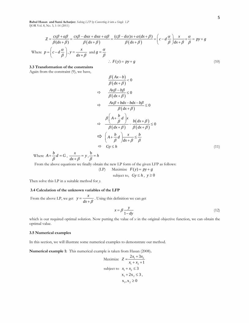
5 Babul Hasan and Sumi Acharjee: Solving LFP by Converting it into a Single LP IJOR Vol. 8, No. 3, 1-14 (2011)
( ) ( )
( ) ( ) ( )
cx cx dx dx c d x dx xc d py gdx dx dx dx
Z β αβ β α α αβ β α α β α αβ β β β β β β β β
+ − + + − + += = = − + = ++ + +
= +
Where c dp αβ
−
= , y x
dx β=
+ and g α
β=
( )F y py g∴ = + (10) 3.3 Transformation of the constraints Again from the constraint (9), we have,
( )( )
0Ax bdx
ββ β
−<
+
( )
0Ax bdxβ β
β β−
≤+
( )
0Ax bdx bdx bdx
β ββ β+ − −
≤+
( )
( )( )
0
bA d xb dx
dx dx
βββ
β β β β
+ + − ≤+ +
b x bA ddxβ β β
+ ≤ +
Gy h≤ (11)
Where bA d Gβ
+ = , x y
dx β=
+,
b hβ=
From the above equations we finally obtain the new LP form of the given LFP as follows: (LP) Maximize ( )F y py g= + subject to, Gy h≤ , 0y ≥ Then solve this LP in a suitable method for y. 3.4 Calculation of the unknown variables of the LFP
From the above LP, we get xy
dx β=
+. Using this definition we can get
1
x ydy
β=−
(12)
which is our required optimal solution. Now putting the value of x in the original objective function, we can obtain the optimal value. 3.5 Numerical examples In this section, we will illustrate some numerical examples to demonstrate our method. Numerical example 1: This numerical example is taken from Hasan (2008).
Maximize 1 2
1 2
2 3
1x x
x xZ +
+ +=
subject to 1 2 3x x+ ≤ 1 2x 2x 3+ ≤ ,
1 2x , x 0≥
6 Babul Hasan and Sumi Acharjee: Solving LFP by Converting it into a Single LP IJOR Vol. 8, No. 3, 1-14 (2011)
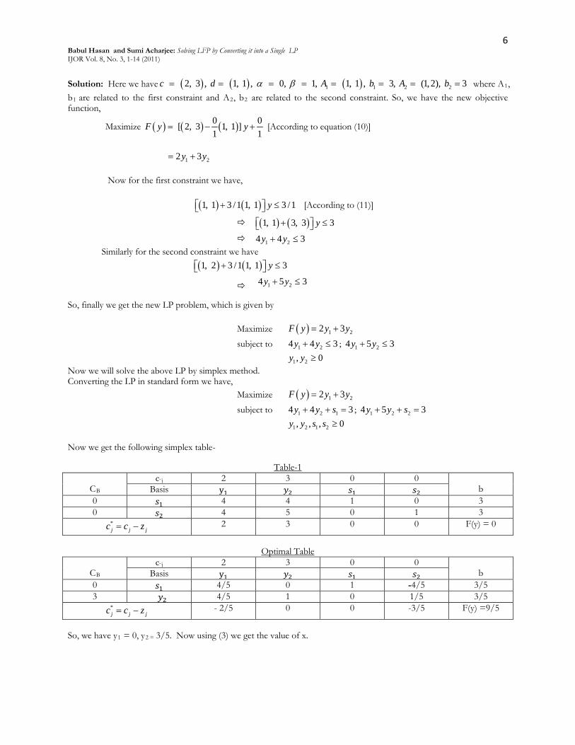
Solution: Here we have ( ) ( ) ( )1 1 2 2 2, 3 , 1, 1 , 0, 1, 1, 1 , 3, (1,2), 3c d A b A bα β= = = = = = = = where A1, b1 are related to the first constraint and A2, b2 are related to the second constraint. So, we have the new objective function,
Maximize ( ) ( ) ( )0 0 [ 2, 3 1, 1 ] 1 1
F y y= − + [According to equation (10)]
1 22 3y y= +
Now for the first constraint we have,
( ) ( ) 1, 1 3 /1 1, 1 3 /1y+ ≤ [According to (11)]
( ) ( )1, 1 3, 3 3y+ ≤
1 24 4 3y y+ ≤ Similarly for the second constraint we have
( ) ( )1, 2 3 /1 1, 1 3y+ ≤
1 24 5 3y y+ ≤ So, finally we get the new LP problem, which is given by Maximize ( ) 1 22 3F y y y+=
subject to 1 24 4 3y y+ ≤ ; 1 24 5 3y y+ ≤ 1 2, 0y y ≥ Now we will solve the above LP by simplex method. Converting the LP in standard form we have, Maximize ( ) 1 22 3F y y y+=
subject to 1 2 1 34 4y y s+ + = ; 1 2 2 34 5y y s+ + = 1 2 1 2, , , 0y y s s ≥ Now we get the following simplex table-
Table-1
CB c j 2 3 0 0
b Basis y1 𝑦2 𝑠1 𝑠2 0 𝑠1 4 4 1 0 3 0 𝑠2 4 5 0 1 3
*j j jc c z= − 2 3 0 0 F(y) = 0
Optimal Table
CB
c j 2 3 0 0 b Basis y1 𝑦2 𝑠1 𝑠2
0 𝑠1 4/5 0 1 -4/5 3/5 3 𝑦2 4/5 1 0 1/5 3/5
*j j jc c z= − - 2/5 0 0 -3/5 F(y) =9/5
So, we have y1 = 0, y2 = 3/5. Now using (3) we get the value of x.
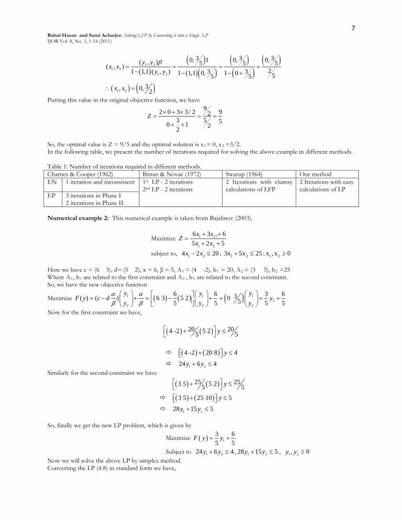
7 Babul Hasan and Sumi Acharjee: Solving LFP by Converting it into a Single LP IJOR Vol. 8, No. 3, 1-14 (2011)
( )
( )( )( )
( )( )
( )1 2
1 21 2
3 3 30, 1 0, 0,( , ) 5 5 5, )23 31 1,1 ( , ) 1 1,1 0, 1 0 55
(5
y yx xy yβ
= = = =− − − +
( ) ( )1 23, 0, 2x x∴ =
Putting this value in the original objective function, we have
92 0 3 3 / 2 92
3 5 50 1 22
Z × + ×= =
+ +=
So, the optimal value is Z = 9/5 and the optimal solution is x1= 0, x2 =3/2. In the following table, we present the number of iterations required for solving the above example in different methods. Table 1: Number of iterations required in different methods. Charnes & Cooper (1962) Bitran & Novae (1972) Swarup (1964) Our method EN 1 iteration and inconsistent 1st LP - 2 iterations
2nd LP - 2 iterations
2 Iterations with clumsy calculations of LFP
2 Iterations with easy calculations of LP
EP 3 iterations in Phase I 2 iterations in Phase II
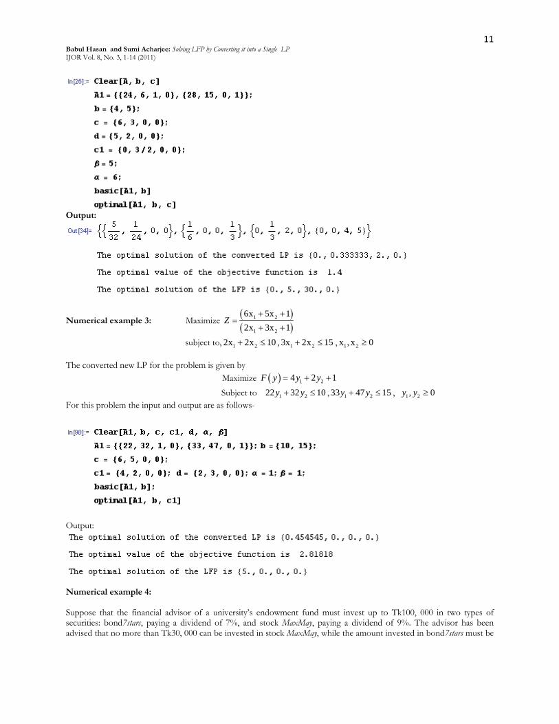
Numerical example 2: This numerical example is taken from Bajalinov (2003).
Maximize 1 2?
1 2
6 3 65 2 5
Zx xx x++
=++
subject to, 1 24 2 20x x− ≤ ; 1 23x 5x 25+ ≤ ; 1 2x , x 0≥ Here we have c = (6 3), d= (5 2), α = 6, β = 5, A1 = (4 -2), b1 = 20, A2 = (3 5), b2 =25 Where A1, b1 are related to the first constraint and A2 , b2 are related to the second constraint. So, we have the new objective function
Maximize ( ) ( ) ( )1 1 12
2 2 2
6 6 3 63( ) ( ) 6 3 5 2 0 55 5 5 5y y y
F y c d yy y y
α αβ β
= − + = − + = = +
Now for the first constraint we have,
( ) ( )20 204 -2 5 25 5y + ≤
( ) ( )4 -2 20 8 4y+ ≤
1 224 6 4y y+ ≤ Similarly for the second constraint we have
( ) ( )25 253 5 5 25 5y + ≤
( ) ( )3 5 25 10 5y+ ≤
1 228 1 55y y+ ≤ So, finally we get the new LP problem, which is given by
Maximize ( ) 13 65 5
F y y= +
Subject to 1 224 6 4y y+ ≤ , 1 228 15 5y y+ ≤ , 1 2, 0y y ≥ Now we will solve the above LP by simplex method. Converting the LP (4.8) in standard form we have,
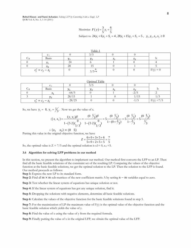
8 Babul Hasan and Sumi Acharjee: Solving LFP by Converting it into a Single LP IJOR Vol. 8, No. 3, 1-14 (2011)
Maximize ( ) 13 65 5
F y y= +
Subject to 1 2 124 6 4y y S+ + = , 1 2 228 15 5y y S+ + = , 1 2 1 2, , , 0y y s s ≥
Table-1 CB
c j 0 3/5 0 0 b Basis y1 𝑦2 𝑠1 𝑠2
0 𝑠1 24 6 1 0 4 0 𝑠2 28 15 0 1 5
𝑐𝑗∗ = 𝑐𝑗 − 𝑧𝑗 0 3/5∆→ 0 0 F(y) = 0
Optimal Table
CB
c j 0 3/5 0 0 b Basis y1 𝑦2 𝑠1 𝑠2
0 𝑠1 -64/5 0 1 -2/5 2 3 𝑦2 28/15 1 0 1/15 1/3
𝑐𝑗∗ = 𝑐𝑗 − 𝑧𝑗 - 28/25 0 0 -1/5 F(y) =7/5 So, we have 1 2
1y 0, y 3= = . Now we get the value of x.
( ( )( ) ( )
1 21 2
(0 ) (0 ) (0 ) (0 )( )5 5 5
0 0 2 21 (0 ) 11 5 2 ( ) 1 5 2 ( ) 3 31/ 3 1/
1 1 1 1 3 3 3 3 1
33
y yx xββ
= = = = =− + −− −
∴ (𝑥1 𝑥2) = (0 5) Putting this value in the original objective function, we have
6 0 3 5 6 75 0 2 5 5 5
Z × + × +=
× + ×=
+
So, the optimal value is Z = 7/5 and the optimal solution is x1= 0, x2 =5. 3.6 Algorithm for solving LFP problems in our method In this section, we present the algorithm to implement our method. Our method first converts the LFP to an LP. Then find all the basic feasible solutions of the constraint set of the resulting LP. Comparing the values of the objective function at the basic feasible solutions, we get the optimal solution to the LP. Then the solution to the LFP is found. Our method proceeds as follows: Step 1: Express the new LP to its standard form. Step 2: Find all m × m sub-matrices of the new coefficient matrix A by setting n − m variables equal to zero.
Step 3: Test whether the linear system of equations has unique solution or not.
Step 4: If the linear system of equations has got any unique solution, find it.
Step 5: Dropping the solutions with negative elements, determine all basic feasible solutions.
Step 6: Calculate the values of the objective function for the basic feasible solutions found in step 5.
Step 7: For the maximization of LP the maximum value of F(y) is the optimal value of the objective function and the basic feasible solution which yields the value of y.
Step 8: Find the value of x using the value of y from the required formula.
Step 9: Finally putting the value of x in the original LFP, we obtain the optimal value of the LFP.
9 Babul Hasan and Sumi Acharjee: Solving LFP by Converting it into a Single LP IJOR Vol. 8, No. 3, 1-14 (2011)
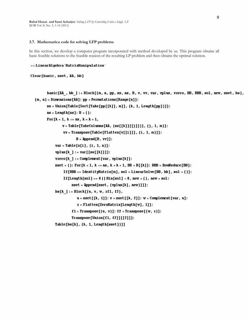
3.7. Mathematica code for solving LFP problems In this section, we develop a computer program incorporated with method developed by us. This program obtains all basic feasible solutions to the feasible reasion of the resulting LP problem and then obtains the optimal solution.
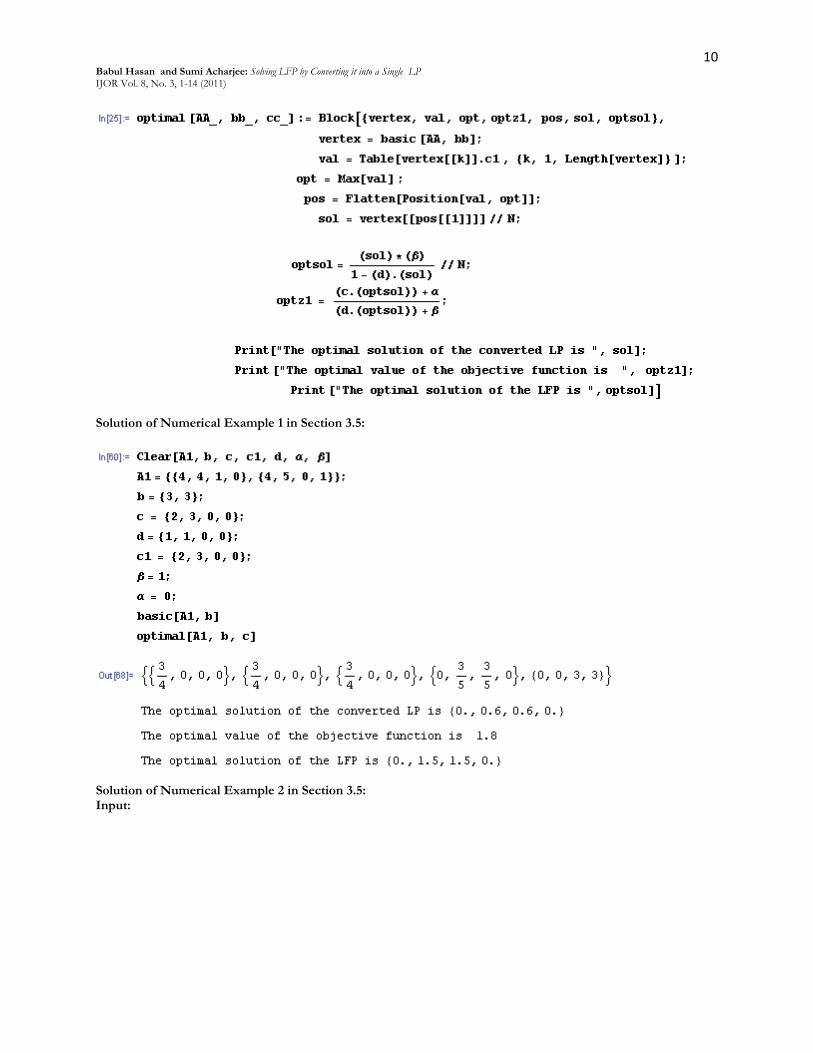
10 Babul Hasan and Sumi Acharjee: Solving LFP by Converting it into a Single LP IJOR Vol. 8, No. 3, 1-14 (2011)
Solution of Numerical Example 1 in Section 3.5:
Solution of Numerical Example 2 in Section 3.5: Input:
11 Babul Hasan and Sumi Acharjee: Solving LFP by Converting it into a Single LP IJOR Vol. 8, No. 3, 1-14 (2011)
Output:
Numerical example 3: Maximize ( )( )
1 2
1 2
6x 5x 12x 3x 1
Z+ ++ +
=
subject to, 1 22x 2x 10+ ≤ , 1 23x 2x 15+ ≤ , 1 2x , x 0≥ The converted new LP for the problem is given by
Maximize ( ) 1 24 2 1F y y y= + +
Subject to 1 222 32 10y y+ ≤ , 1 233 47 15y y+ ≤ , 1 2, 0y y ≥ For this problem the input and output are as follows-
Output:
Numerical example 4: Suppose that the financial advisor of a university’s endowment fund must invest up to Tk100, 000 in two types of securities: bond7stars, paying a dividend of 7%, and stock MaxMay, paying a dividend of 9%. The advisor has been advised that no more than Tk30, 000 can be invested in stock MaxMay, while the amount invested in bond7stars must be
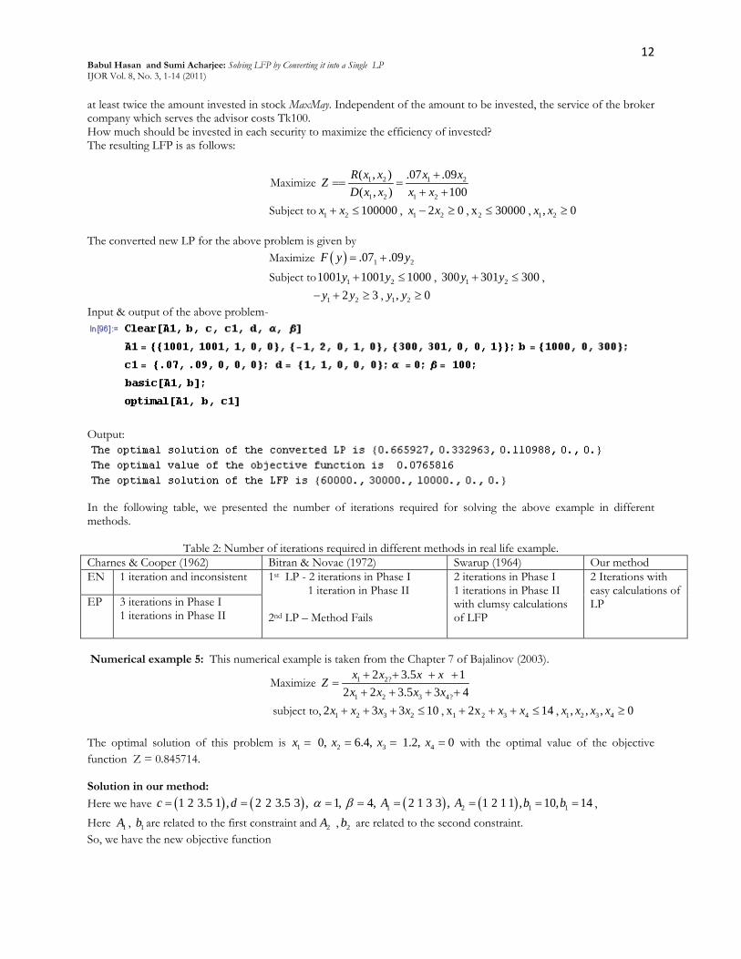
12 Babul Hasan and Sumi Acharjee: Solving LFP by Converting it into a Single LP IJOR Vol. 8, No. 3, 1-14 (2011)
at least twice the amount invested in stock MaxMay. Independent of the amount to be invested, the service of the broker company which serves the advisor costs Tk100. How much should be invested in each security to maximize the efficiency of invested? The resulting LFP is as follows:
Maximize 1 2 1 2
1 2 1 2
( , ) . .07(
09, ) 100
R x x x xD x x x x
Z =+
=+
+=
Subject to 1 2 100000x x+ ≤ , 1 22 0x x− ≥ , 2x 30000≤ , 1 2, 0x x ≥ The converted new LP for the above problem is given by
Maximize ( ) 1 2.07 .09F y y= +
Subject to 1 21001 1001 1000y y+ ≤ , 1 2300 301 300y y+ ≤ , 1 22 3y y− + ≥ , 1 2, 0y y ≥ Input & output of the above problem-
Output:
In the following table, we presented the number of iterations required for solving the above example in different methods.
Table 2: Number of iterations required in different methods in real life example. Charnes & Cooper (1962) Bitran & Novae (1972) Swarup (1964) Our method EN 1 iteration and inconsistent 1st LP - 2 iterations in Phase I
1 iteration in Phase II 2nd LP – Method Fails
2 iterations in Phase I 1 iterations in Phase II with clumsy calculations of LFP
2 Iterations with easy calculations of LP EP 3 iterations in Phase I
1 iterations in Phase II
Numerical example 5: This numerical example is taken from the Chapter 7 of Bajalinov (2003).
Maximize 1 2?
1 2 3 4?
2 3.5 12 2 3.5 3 4
x x x xx x
Zx x
+ + + ++ + + +
=
subject to, 1 2 3 22 3 3 10x x x x+ + + ≤ , 1 2 3 4x 2x 14x x+ + + ≤ , 1 2 3 4,, 0, x xx x ≥ The optimal solution of this problem is 1 2 3 4 0, 6.4, 1.2, 0x x x x= = = = with the optimal value of the objective function Z = 0.845714. Solution in our method: Here we have ( ) ( ) ( ) ( )1 2 1 11 2 3.5 1 , 2 2 3.5 3 , 1, 4, 2 1 3 3 , 1 2 1 1 , 10, 14c d A A b bα β= = = = = = = = ,
Here 1A , 1b are related to the first constraint and 2A , 2b are related to the second constraint. So, we have the new objective function
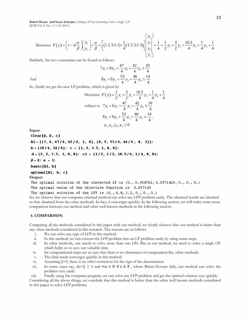
13 Babul Hasan and Sumi Acharjee: Solving LFP by Converting it into a Single LP IJOR Vol. 8, No. 3, 1-14 (2011)
Maximize ( ) ( ) ( )
1
1 21 2 3 4
2 3
4
1 1 1 3 10.5 1 11 2 3.5 1 - 2 2 3.5 34 4 2 2 4 4 4
yy y
F y c d y y y yy y
y
α αβ β
= − + = + = + + + +
Similarly, the two constraints can be found as follows:
1 2 3 447 42 107 64 4 4
y y y y+ + + ≤
And 1 2 3 453 46 148 94 4 4
y y y y+ + + ≤
So, finally we get the new LP problem, which is given by
Maximize ( ) 1 2 3 41 3 10.5 1 12 2 4 4 4
F y y y y y= + + + +
subject to 1 2 3 447 42 107 64 4 4
y y y y+ + + ≤
1 2 3 453 46 148 94 4 4
y y y y+ + + ≤ ,
1 2 3 4, , , 0y y y y ≥ Input:
Output:
So, we observe that our computer oriented method can solve any LFP problem easily. The obtained results are identical to that obtained from the other methods. In fact, it converges quickly. In the following section, we will make some more comparison between our method and other well-known methods in the following section. 4. COMPARISON Comparing all the methods considered in this paper with our method, we clearly observe that our method is better than any other methods considered in this research. The reasons are as follows-
i. We can solve any type of LFP in this method. ii. In this method, we can convert the LFP problem into an LP problem easily by using some steps. iii. In other methods, one needs to solve more than one LPs. But in our method, we need to solve a single LP,
which helps us to save our valuable time. iv. Its computational steps are so easy that there is no clumsiness of computation like other methods. v. The final result converges quickly in this method. vi. Assuming β>0, there is no other restriction for the sign of the denominator. vii. In some cases say, dx+β ≥ 0 and +𝛼 < 0 ∀ 𝑥 ∈ 𝑋 , where Bitran-Novaes fails, our method can solve the
problem very easily. viii. Finally using the computer program, we can solve any LFP problem and get the optimal solution very quickly.
Considering all the above things, we conclude that this method is better than the other well known methods considered in this paper to solve LFP problems.
14 Babul Hasan and Sumi Acharjee: Solving LFP by Converting it into a Single LP IJOR Vol. 8, No. 3, 1-14 (2011)
5. CONCLUSION Our aim was to develop an easy technique for solving LFP problems. So in this paper, we have introduced a computer oriented technique which converts the LFP problem into a single LP problem. We developed this computer technique by using programming language MATHEMATICA. We also highlighted the limitations of different methods. We illustrate a number of numerical examples to demonstrate our method. We then compare our method with other existing methods in the literature for solving LFP problems. From this comparison, we observed that our method gave identical result with that obtained by the other methods easily. So, we conclude that, this method is better than the other well known methods considered in this paper for solving LFP problems. ACKNOWLEDGEMENTS The authors are very grateful to the anonymous referees for their valuable comments and suggestions to improve the paper in the present form. REFERENCES
1. Bajalinov, E. B. (2003). Linear-Fractional Programming: Theory, Methods, Applications and Software. Boston: Kluwer Academic Publishers.
2. Bitran, G. R. and Novaes, A. G. (1972). Linear Programming with a Fractional Objective Function, University of Sao Paulo, Brazil. 21: 22-29
3. Charnes, A. and Cooper, W.W. (1962). Programming with linear fractional functions, Naval Research Logistics Quarterly, 9: 181-186.
4. Charnes, A., Cooper, W. W. (1973). An explicit general solution in linear fractional programming, Naval Research Logistics Quarterly, 20(3): 449-467.
5. Dantzig, G.B. (1962). Linear Programming and extension, Princeton University Press, Princeton, N.J. 6. Hasan, M. B., (2008). Solution of Linear Fractional Programming Problems through Computer Algebra, The
Dhaka University Journal of Science, 57(1): 23-28. 7. Hasan, M. B., Khodadad Khan, A. F. M. and Ainul Islam, M. (2001). Basic Solutions of Linear System of Equations
through Computer Algebra, Journal Bangladesh Mathematical Society. 21: 39-45. 8. Harvey, M. W. and John, S. C. Y. (1968). Algorithmic Equivalence in Linear Fractional Programming, Management
Science, 14(5): 301-306. 9. Martos, B. (1960). Hyperbolic Programming, Publications of the Research Institute for Mathematical Sciences, Hungarian
Academy of Sciences, 5(B): 386-407. 10. Martos, B. (1964). Hyperbolic Programming, Naval Research Logistics Quarterly, 11: 135-155. 11. Swarup, K. (1964). Linear fractional functional programming, Operations Research, 13(6): 1029-1036. 12. Swarup, K., Gupta, P. K. and Mohan, M. (2003). Tracts in Operation Research, Eleventh Thoroughly Revised Edition,
ISBN: 81-8054-059-6. 13. Tantawy, S. F. (2007). A New Method for Solving Linear Fractional Programming problems, Australian Journal of
Basic and Applied Science, INSInet Publications. 1(2): 105-108. 14. Wolfram, S. (2000). Mathematica Addision-Wesly Publishing Company, Melno Park, California, New York.