Small Angle Neutron Scattering Part 4Polymers and Biological systems

(R.K.Heenan, with thanks to Steve King, ISIS, for use of some of his slides)

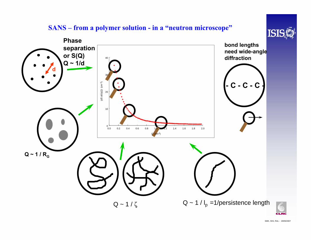
SANS – from a polymer solution - in a “neutron microscope”

SMK, ISIS, RAL - 29/05/2007

- C - C - C -

Phase separationor S(Q)Q ~ 1/d

Q ~ 1 / RG

Q ~ 1 / ζ Q ~ 1 / lp =1/persistence length

bond lengthsneed wide-angle diffraction

0.0 0.2 0.4 0.6 0.8 1.0 1.2 1.4 1.6 1.8 2.0

Q (nm-1)

0

10

20

30

40

(dΣ/

dΩ)(Q

) (c

m-1

)

d

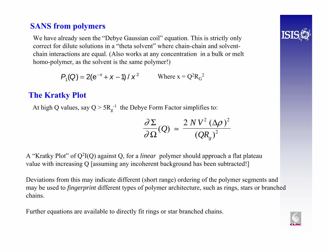
The Kratky Plot

∂∂

ρΣΩ

Δ( )

( )( )

QN V

QRg≈

2 2 2

2

At high Q values, say Q > 5Rg-1 the Debye Form Factor simplifies to:

A “Kratky Plot” of Q2I(Q) against Q, for a linear polymer should approach a flat plateau value with increasing Q [assuming any incoherent background has been subtracted!]

Deviations from this may indicate different (short range) ordering of the polymer segments and may be used to fingerprint different types of polymer architecture, such as rings, stars or branched chains.

Further equations are available to directly fit rings or star branched chains.

SANS from polymersWe have already seen the “Debye Gaussian coil” equation. This is strictly only correct for dilute solutions in a “theta solvent” where chain-chain and solvent-chain interactions are equal. (Also works at any concentration in a bulk or melt homo-polymer, as the solvent is the same polymer!)

P Q x xx1

22 1( ) (e ) /= + −− Where x = Q2RG2

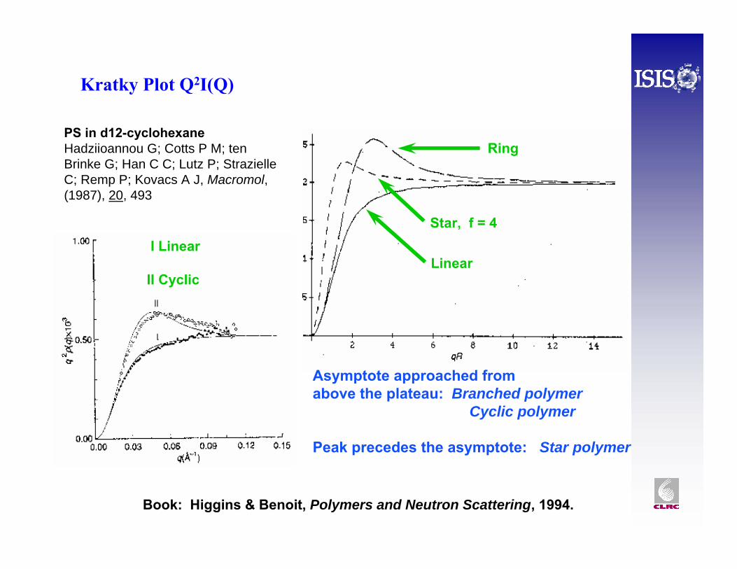
Book: Higgins & Benoit, Polymers and Neutron Scattering, 1994.

Linear

Ring

Star, f = 4I Linear

II Cyclic

PS in d12-cyclohexaneHadziioannou G; Cotts P M; ten Brinke G; Han C C; Lutz P; StrazielleC; Remp P; Kovacs A J, Macromol, (1987), 20, 493

Asymptote approached from above the plateau: Branched polymer

Cyclic polymer

Peak precedes the asymptote: Star polymer

Kratky Plot Q2I(Q)

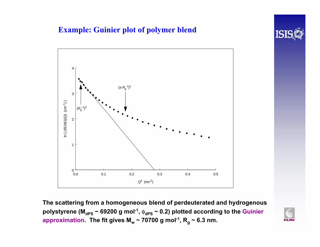
Example: Guinier plot of polymer blend

0.0 0.1 0.2 0.3 0.4 0.5

Q2 (nm-2)

0

1

2

3

4ln

[ (d

Σ/dΩ

)(Q)

(cm

-1) ]

(Rg-1)2

(π Rg-1)2

The scattering from a homogeneous blend of perdeuterated and hydrogenous polystyrene (MdPS ~ 69200 g mol-1, φdPS ~ 0.2) plotted according to the Guinierapproximation. The fit gives Mw ~ 70700 g mol-1, Rg ~ 6.3 nm.

The Zimm Approximation (at higher concentrations)As the polymer concentration c increases, but is still less than the overlap concentration c*, P(Q) gets pushed down, but instead of using I(Q)=P(Q)S(Q) we have:

Where c = concentration, M = molecular weight, d = bulk density, P1(Q) is the Debye Gaussian coil equation, and A2 is the “second virial coefficient”.

In the Guinier range, at low Q, a “Zimm Plot” of 1/I(Q) against Q2 gives M and RG.

Swollen coils

In a “good solvent” the polymer coil may expand, so that at intermediate Q there is no longer a Q-2 dependence. Instead:

Where in a “good solvent” ν = 3/5 compared to ½ for a theta solvent.

ν/1)( −∝ QQP

...])(2)([)( 2121 +−= QcMPAQPkcMQI 2

2

dN

kA

ρΔ=

⎟⎟⎠

⎞⎜⎜⎝

⎛+++

Δ≈ ...21

3)()(1

2

22

2

2

cMARQcM

dNQI

GA

ρ

Zimm Plot (at low concentration)

intercept = × = ×1 12

2 2MN

c MNA Aδ

ρδ

φ ρ( ) ( )Δ Δ

gradient = ×Rg

2

3intercept

Zimm B, J Chem Phys, (1948), 16, 1093

For a DILUTE solution (or in a bulk homopolymer) we can ignore the A2 term and use a straight line fit to a Zimm plot to get M and RG

[ Note that there are a few polymers where D- and H- chains do have different interaction parameters and phase separation my occur.]

0.0 0.1 0.2 0.3 0.4 0.5

Q2 (nm-2)

0.0

0.1

0.2

0.3[ (

dΣ/d

Ω)(Q

) ]-1

(cm

)

(Rg-1)2

(π Rg-1)2

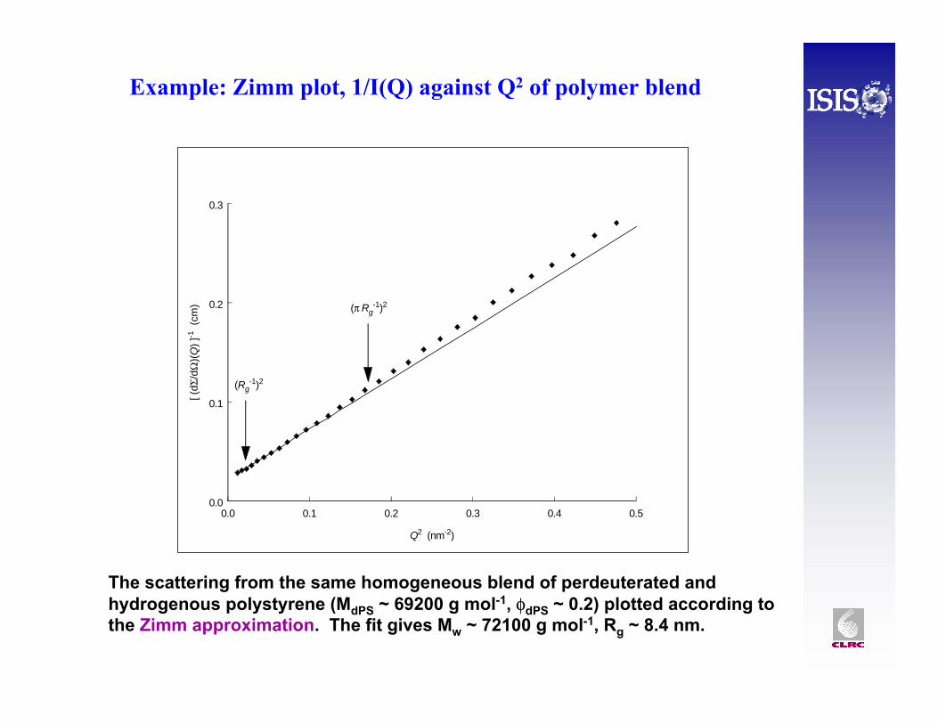
The scattering from the same homogeneous blend of perdeuterated and hydrogenous polystyrene (MdPS ~ 69200 g mol-1, φdPS ~ 0.2) plotted according to the Zimm approximation. The fit gives Mw ~ 72100 g mol-1, Rg ~ 8.4 nm.

Example: Zimm plot, 1/I(Q) against Q2 of polymer blend

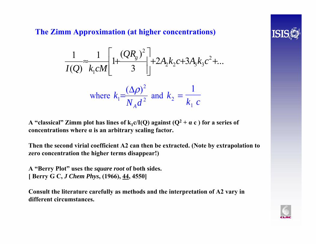
...323

)(11

)(1 2

3322

2

1

+++⎥⎥⎦

⎤

⎢⎢⎣

⎡+≈ ckAckA

QRMckQI

g

where 2

2

1)(

dNk

A

ρΔ= and kk c2

1

1=

A “classical” Zimm plot has lines of k1c/I(Q) against (Q2 + α c ) for a series of concentrations where α is an arbitrary scaling factor.

Then the second virial coefficient A2 can then be extracted. (Note by extrapolation tozero concentration the higher terms disappear!)

A “Berry Plot” uses the square root of both sides.[ Berry G C, J Chem Phys, (1966), 44, 4550]

Consult the literature carefully as methods and the interpretation of A2 vary in different circumstances.

The Zimm Approximation (at higher concentrations)

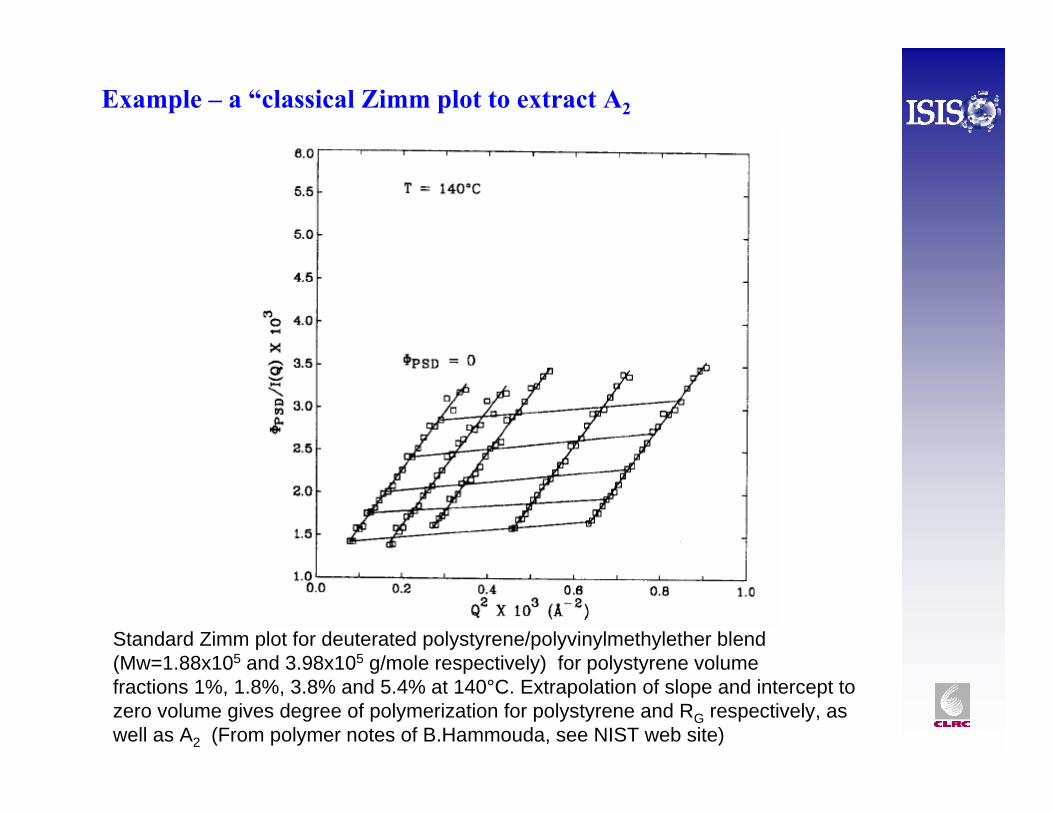
Example – a “classical Zimm plot to extract A2

Standard Zimm plot for deuterated polystyrene/polyvinylmethylether blend(Mw=1.88x105 and 3.98x105 g/mole respectively) for polystyrene volumefractions 1%, 1.8%, 3.8% and 5.4% at 140°C. Extrapolation of slope and intercept to zero volume gives degree of polymerization for polystyrene and RG respectively, as well as A2 (From polymer notes of B.Hammouda, see NIST web site)

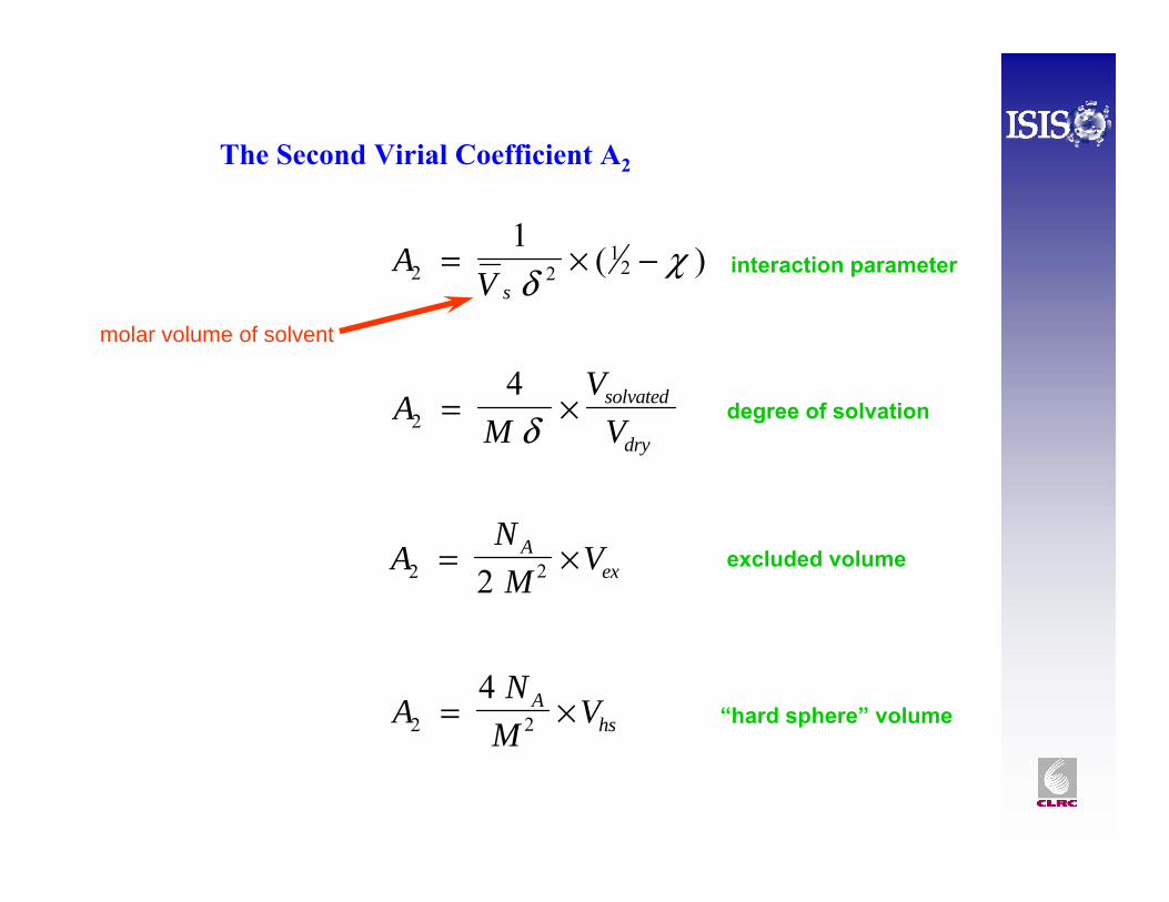
The Second Virial Coefficient A2

ANM

VAex2 22

= ×

AV s

2 21

21

= × −δ

χ( )

AM

VVsolvated

dry2

4= ×δ

AN

MVA

hs2 2

4= ×

excluded volume

“hard sphere” volume

degree of solvation

interaction parameter

molar volume of solvent

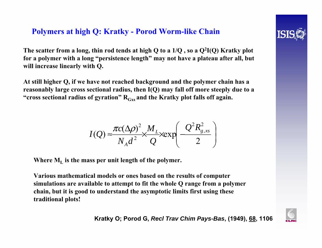
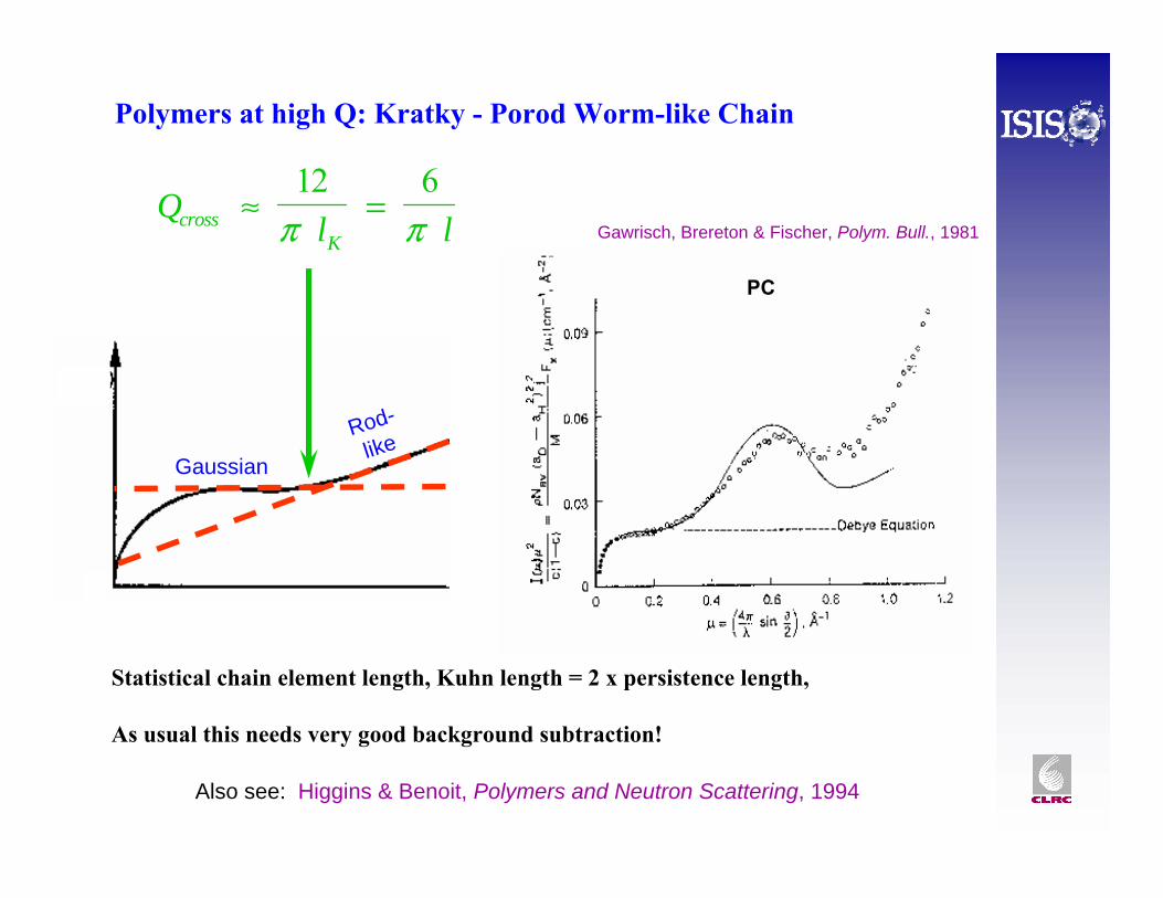
Polymers at high Q: Kratky - Porod Worm-like Chain

The scatter from a long, thin rod tends at high Q to a 1/Q , so a Q2I(Q) Kratky plot for a polymer with a long “persistence length” may not have a plateau after all, but will increase linearly with Q.

At still higher Q, if we have not reached background and the polymer chain has a reasonably large cross sectional radius, then I(Q) may fall off more steeply due to a “cross sectional radius of gyration” RGxs and the Kratky plot falls off again.

Kratky O; Porod G, Recl Trav Chim Pays-Bas, (1949), 68, 1106

⎟⎟⎠

⎞⎜⎜⎝

⎛−××Δ≈

2exp)()(

2,

2

2

2xsgL

A

RQQ

MdN

cQI ρπ

Where ML is the mass per unit length of the polymer.

Various mathematical models or ones based on the results of computer simulations are available to attempt to fit the whole Q range from a polymer chain, but it is good to understand the asymptotic limits first using these traditional plots!

Also see: Higgins & Benoit, Polymers and Neutron Scattering, 1994

Ql lcross

K≈ =

12 6π π

Rod-like

Gaussian

Gawrisch, Brereton & Fischer, Polym. Bull., 1981

PC

Polymers at high Q: Kratky - Porod Worm-like Chain

Statistical chain element length, Kuhn length = 2 x persistence length,

As usual this needs very good background subtraction!

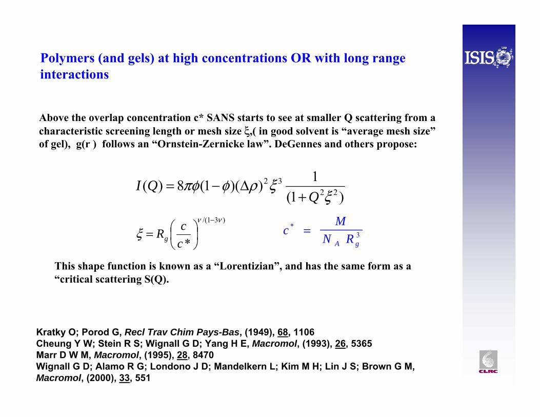
Polymers (and gels) at high concentrations OR with long range interactions

Above the overlap concentration c* SANS starts to see at smaller Q scattering from a characteristic screening length or mesh size ξ,( in good solvent is “average mesh size”of gel), g(r ) follows an “Ornstein-Zernicke law”. DeGennes and others propose:

This shape function is known as a “Lorentizian”, and has the same form as a “critical scattering S(Q).

cM

N RA g

* = 3

)31/(

*

νν

ξ−

⎟⎠⎞

⎜⎝⎛=

ccRg

)1(1))(1(8)( 22

32

ξξρφπφ

QQI

+Δ−=

Kratky O; Porod G, Recl Trav Chim Pays-Bas, (1949), 68, 1106Cheung Y W; Stein R S; Wignall G D; Yang H E, Macromol, (1993), 26, 5365Marr D W M, Macromol, (1995), 28, 8470Wignall G D; Alamo R G; Londono J D; Mandelkern L; Kim M H; Lin J S; Brown G M, Macromol, (2000), 33, 551

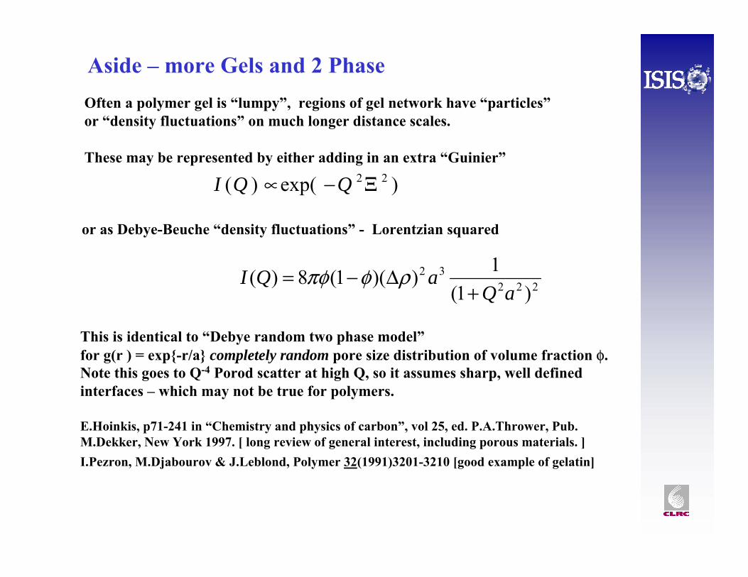
Aside – more Gels and 2 Phase

or as Debye-Beuche “density fluctuations” - Lorentzian squared

This is identical to “Debye random two phase model”for g(r ) = exp{-r/a} completely random pore size distribution of volume fraction φ. Note this goes to Q-4 Porod scatter at high Q, so it assumes sharp, well defined interfaces – which may not be true for polymers.

E.Hoinkis, p71-241 in “Chemistry and physics of carbon”, vol 25, ed. P.A.Thrower, Pub. M.Dekker, New York 1997. [ long review of general interest, including porous materials. ]I.Pezron, M.Djabourov & J.Leblond, Polymer 32(1991)3201-3210 [good example of gelatin]

22232

)1(1))(1(8)(

aQaQI

+Δ−= ρφπφ

Often a polymer gel is “lumpy”, regions of gel network have “particles”or “density fluctuations” on much longer distance scales.

These may be represented by either adding in an extra “Guinier”

)exp()( 22Ξ−∝ QQI

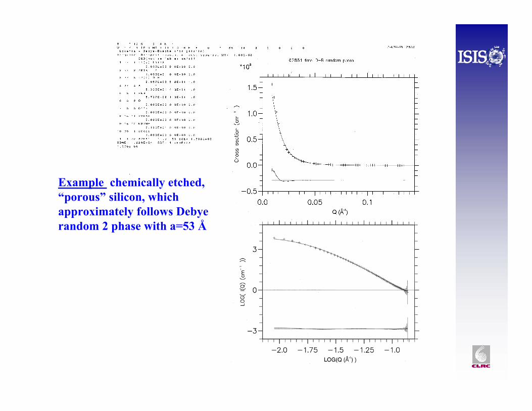
Example chemically etched, “porous” silicon, which approximately follows Debyerandom 2 phase with a=53 Å

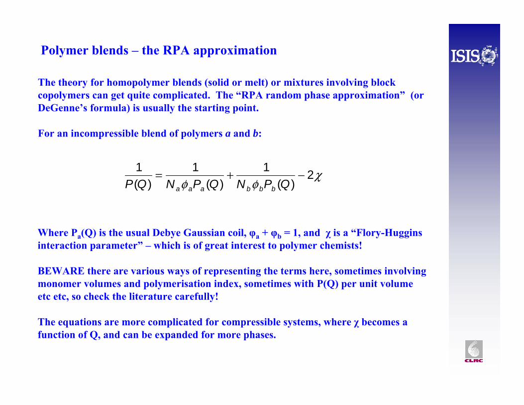
Polymer blends – the RPA approximation

The theory for homopolymer blends (solid or melt) or mixtures involving block copolymers can get quite complicated. The “RPA random phase approximation” (or DeGenne’s formula) is usually the starting point.

For an incompressible blend of polymers a and b:

1 1 1 2P Q N P Q N P Qa a a b b b( ) ( ) ( )

= + −φ φ

χ

Where Pa(Q) is the usual Debye Gaussian coil, φa + φb = 1, and χ is a “Flory-Huggins interaction parameter” – which is of great interest to polymer chemists!

BEWARE there are various ways of representing the terms here, sometimes involving monomer volumes and polymerisation index, sometimes with P(Q) per unit volume etc etc, so check the literature carefully!

The equations are more complicated for compressible systems, where χ becomes a function of Q, and can be expanded for more phases.

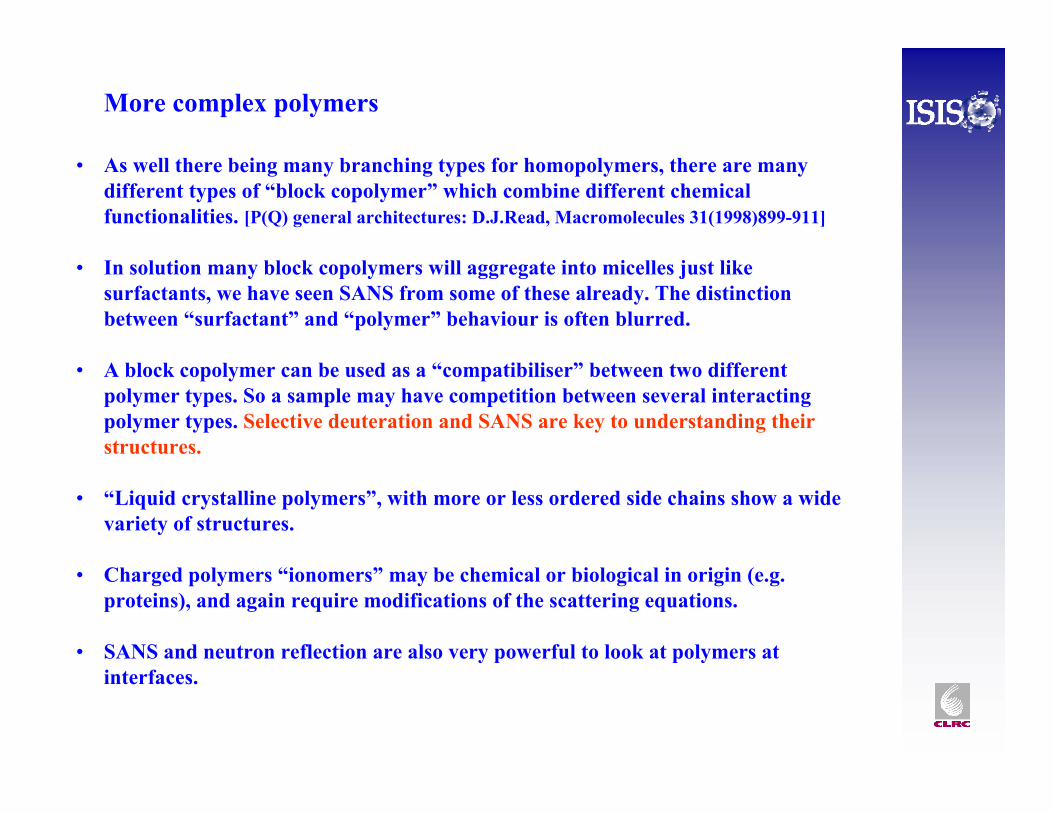
More complex polymers

• As well there being many branching types for homopolymers, there are many different types of “block copolymer” which combine different chemical functionalities. [P(Q) general architectures: D.J.Read, Macromolecules 31(1998)899-911]

• In solution many block copolymers will aggregate into micelles just like surfactants, we have seen SANS from some of these already. The distinction between “surfactant” and “polymer” behaviour is often blurred.

• A block copolymer can be used as a “compatibiliser” between two different polymer types. So a sample may have competition between several interacting polymer types. Selective deuteration and SANS are key to understanding their structures.

• “Liquid crystalline polymers”, with more or less ordered side chains show a wide variety of structures.

• Charged polymers “ionomers” may be chemical or biological in origin (e.g. proteins), and again require modifications of the scattering equations.

• SANS and neutron reflection are also very powerful to look at polymers at interfaces.

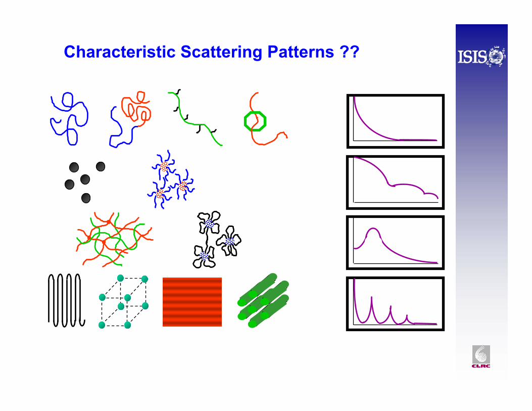
Characteristic Scattering Patterns ??

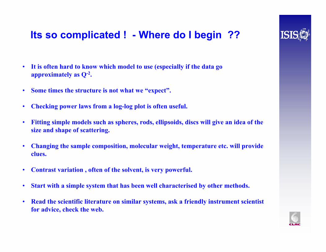
• It is often hard to know which model to use (especially if the data go approximately as Q-2.

• Some times the structure is not what we “expect”.

• Checking power laws from a log-log plot is often useful.

• Fitting simple models such as spheres, rods, ellipsoids, discs will give an idea of the size and shape of scattering.

• Changing the sample composition, molecular weight, temperature etc. will provide clues.

• Contrast variation , often of the solvent, is very powerful.

• Start with a simple system that has been well characterised by other methods.

• Read the scientific literature on similar systems, ask a friendly instrument scientist for advice, check the web.

Its so complicated ! - Where do I begin ??

Polymers at surfaces

• In a previous talk we saw that SANS is sensitive to density profiles at a spherical shell surface, especially if the core particle can be contrast matched to the solvent.

• Polymers are often used as steric stabilisers for liquid droplets or solid particles. Understanding the structure of this layer is important to improve product performance – such as paint, or drug delivery systems or artificial blood.

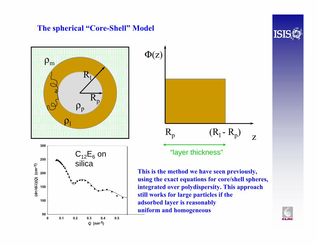
The spherical “Core-Shell” Model

Φ(z)

zRp (Rl - Rp)

Rp

Rl

ρl

ρp

ρm

0 0.1 0.2 0.3 0.4 0.5Q (nm-1)

50

100

150

200

250

300

(dσ

/dΩ

)(Q)

(cm

-1)

C12E6 on silica

This is the method we have seen previously, using the exact equations for core/shell spheres, integrated over polydispersity. This approach still works for large particles if theadsorbed layer is reasonablyuniform and homogeneous

“layer thickness”

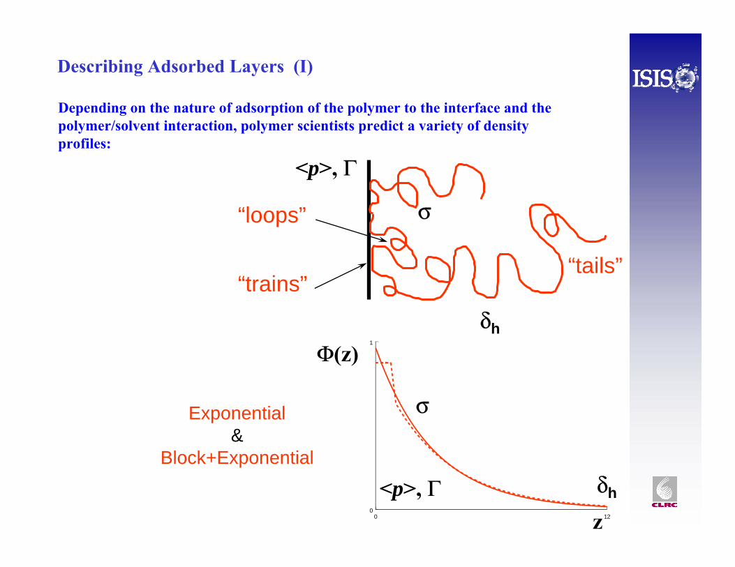
Describing Adsorbed Layers (I)

0 120

1

z

Φ(z)

δh

σ

<p>, Γ

“trains”

“loops”

“tails”

δh

σ

<p>, Γ

Exponential&

Block+Exponential

Depending on the nature of adsorption of the polymer to the interface and the polymer/solvent interaction, polymer scientists predict a variety of density profiles:

0 120

1

Φ(z)

z

Gaussian&

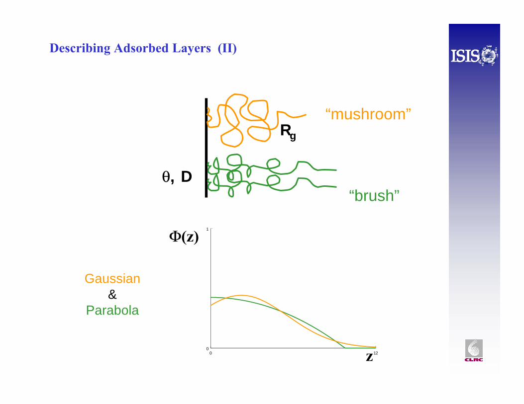
Parabola

“brush”

“mushroom”

θ, D

Rg

Describing Adsorbed Layers (II)

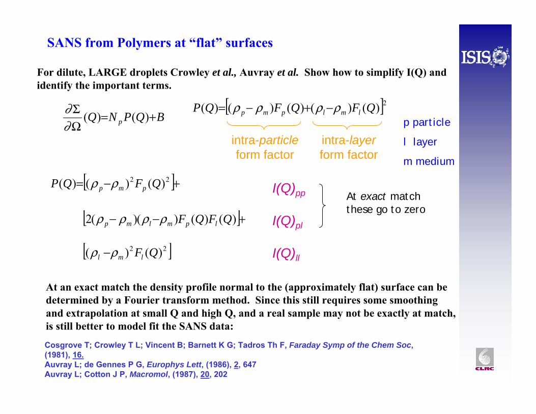
SANS from Polymers at “flat” surfaces

BQPNQ p +=ΩΣ )()(

∂∂

[ ]+−= 22 )()()( QFQP pmp ρρ

[ ]+−− )()()()(2 QFQF lpmlmp ρρρρ

[ ]22 )()( QFlml ρρ −

[ ]2)()()()()( QFQFQP lmlpmp ρρρρ −+−=

intra-particleform factor

intra-layerform factor

I(Q)pp

I(Q)pl

I(Q)ll

For dilute, LARGE droplets Crowley et al., Auvray et al. Show how to simplify I(Q) and identify the important terms.

p particle

l layer

m medium

At exact match these go to zero

At an exact match the density profile normal to the (approximately flat) surface can be determined by a Fourier transform method. Since this still requires some smoothing and extrapolation at small Q and high Q, and a real sample may not be exactly at match, is still better to model fit the SANS data:

Cosgrove T; Crowley T L; Vincent B; Barnett K G; Tadros Th F, Faraday Symp of the Chem Soc, (1981), 16.Auvray L; de Gennes P G, Europhys Lett, (1986), 2, 647Auvray L; Cotton J P, Macromol, (1987), 20, 202

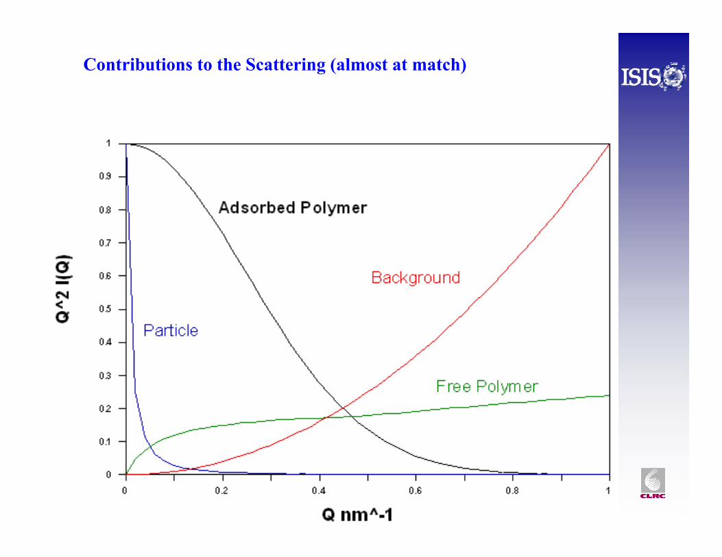
Contributions to the Scattering (almost at match)

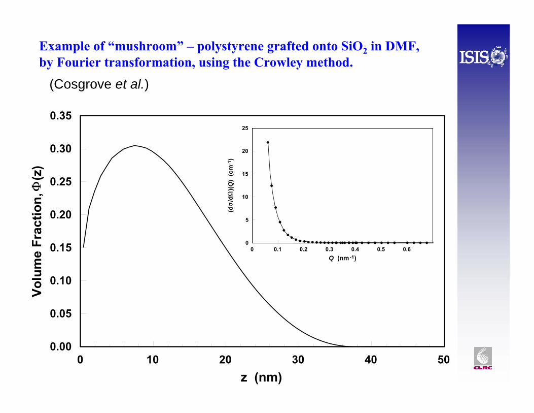
Example of “mushroom” – polystyrene grafted onto SiO2 in DMF,by Fourier transformation, using the Crowley method.

0 10 20 30 40 50z (nm)

0.00

0.05

0.10

0.15

0.20

0.25

0.30

0.35

Volu

me

Frac

tion,

Φ(z

)

0 0.1 0.2 0.3 0.4 0.5 0.6Q (nm -1)

0

5

10

15

20

25

(dσ

/dΩ

)(Q)

(cm

-1)

(Cosgrove et al.)

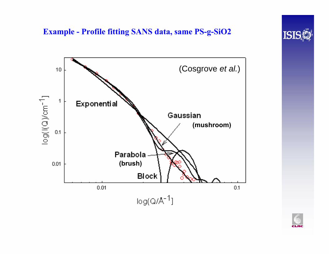
Example - Profile fitting SANS data, same PS-g-SiO2

(Cosgrove et al.)

(mushroom)

(brush)

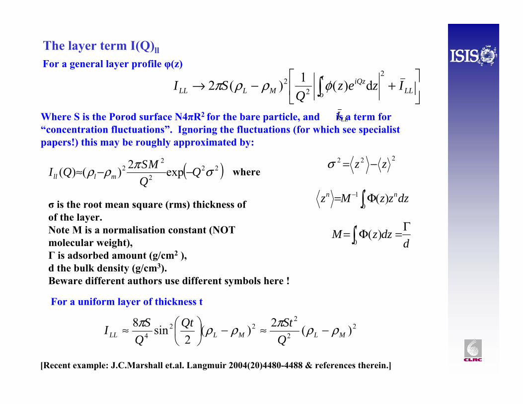
The layer term I(Q)ll

∫Γ=Φ=

t

ddzzM

0)(

( )222

22 exp2)()( σπρρ Q

QMSQI mlll −−≈

222 zz −=σ

dzzzMzt nn ∫ Φ= −

0

1 )(

where

⎥⎦

⎤⎢⎣

⎡ +−→ ∫ LL

t

o

iQzMLLL Izez

QSI

2

22 d)(1)(2 φρρπ

For a general layer profile φ(z)

Where S is the Porod surface N4πR2 for the bare particle, and is a term for “concentration fluctuations”. Ignoring the fluctuations (for which see specialist papers!) this may be roughly approximated by:

LLI

σ is the root mean square (rms) thickness of of the layer.Note M is a normalisation constant (NOTmolecular weight), Γ is adsorbed amount (g/cm2 ),d the bulk density (g/cm3). Beware different authors use different symbols here !

For a uniform layer of thickness t

22

222

4 )(2)(2

sin8MLMLLL Q

StQtQ

SI ρρπρρπ −≈−⎟⎠⎞

⎜⎝⎛≈

[Recent example: J.C.Marshall et.al. Langmuir 2004(20)4480-4488 & references therein.]

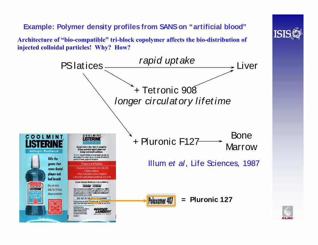
Architecture of “bio-compatible” tri-block copolymer affects the bio-distribution of injected colloidal particles! Why? How?

Illum et al, Life Sciences, 1987

PS latices Liver

+ Tetronic 908longer circulatory lifetime

rapid uptake

+ Pluronic F127Bone

Marrow

Example: Polymer density profiles from SANS on “artificial blood”

= Pluronic 127

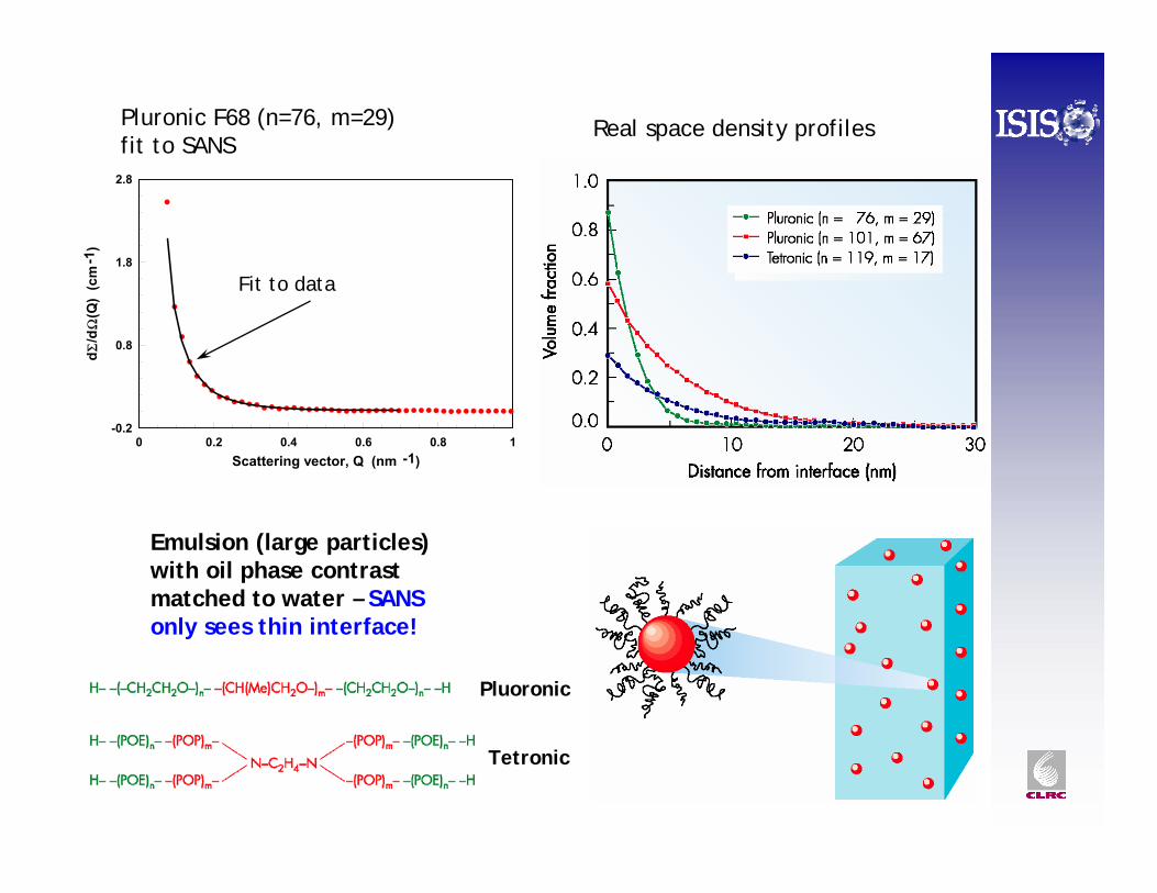
0 0.2 0.4 0.6 0.8 1Scattering vector, Q (nm -1)

-0.2

0.8

1.8

2.8

d Σ/d

Ω(Q

) (c

m-1

)

Fit to data

Pluronic F68 (n=76, m=29)fit to SANS

Real space density profiles

Pluoronic

Tetronic

Emulsion (large particles) with oil phase contrast matched to water – SANS only sees thin interface!

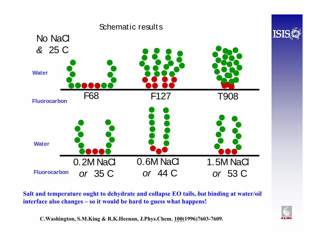
F68 F127

0.2M NaClor 35 C

0.6M NaClor 44 C

1.5M NaClor 53 C

No NaCl& 25 C

T908

Schematic results

Water

Fluorocarbon

Water

Fluorocarbon

C.Washington, S.M.King & R.K.Heenan, J.Phys.Chem. 100(1996)7603-7609.

Salt and temperature ought to dehydrate and collapse EO tails, but binding at water/oil interface also changes – so it would be hard to guess what happens!

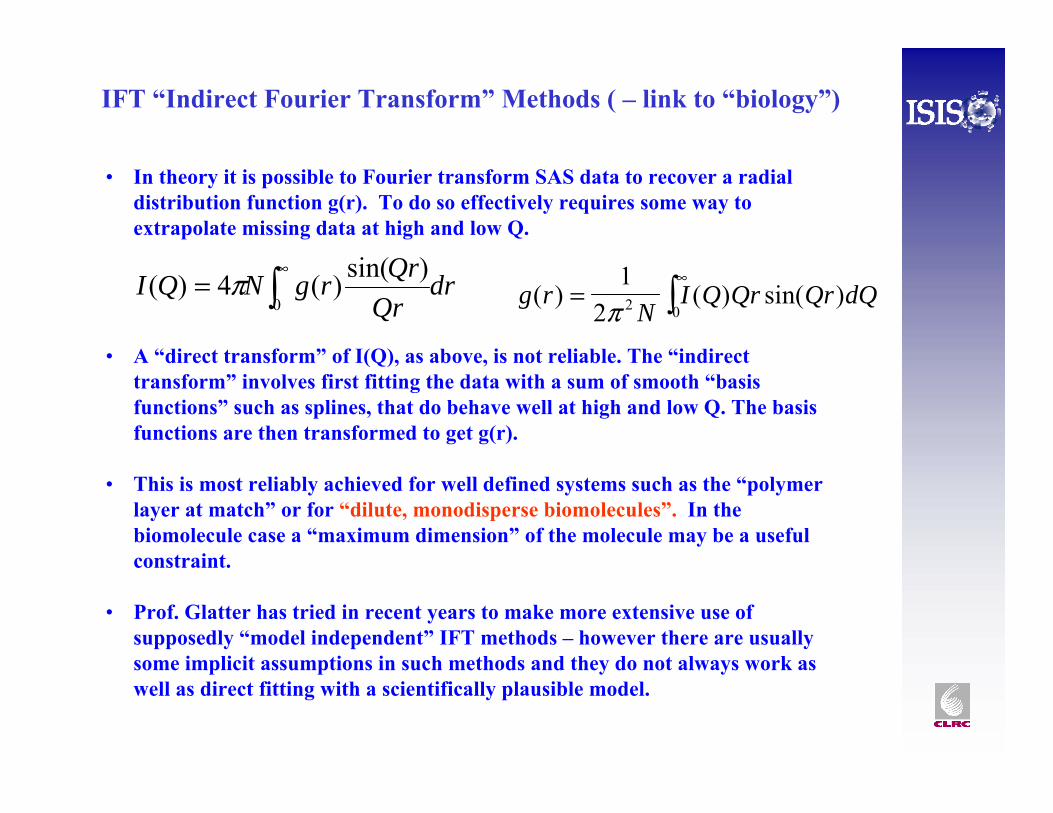
IFT “Indirect Fourier Transform” Methods ( – link to “biology”)

• In theory it is possible to Fourier transform SAS data to recover a radial distribution function g(r). To do so effectively requires some way to extrapolate missing data at high and low Q.

• A “direct transform” of I(Q), as above, is not reliable. The “indirect transform” involves first fitting the data with a sum of smooth “basis functions” such as splines, that do behave well at high and low Q. The basis functions are then transformed to get g(r).

• This is most reliably achieved for well defined systems such as the “polymer layer at match” or for “dilute, monodisperse biomolecules”. In the biomolecule case a “maximum dimension” of the molecule may be a useful constraint.

• Prof. Glatter has tried in recent years to make more extensive use of supposedly “model independent” IFT methods – however there are usually some implicit assumptions in such methods and they do not always work as well as direct fitting with a scientifically plausible model.

g rN

I Q Qr Qr dQ( ) ( ) sin( )=∞

∫1

2 2 0π∫∞

=0

)sin()(4)( drQr

QrrgNQI π

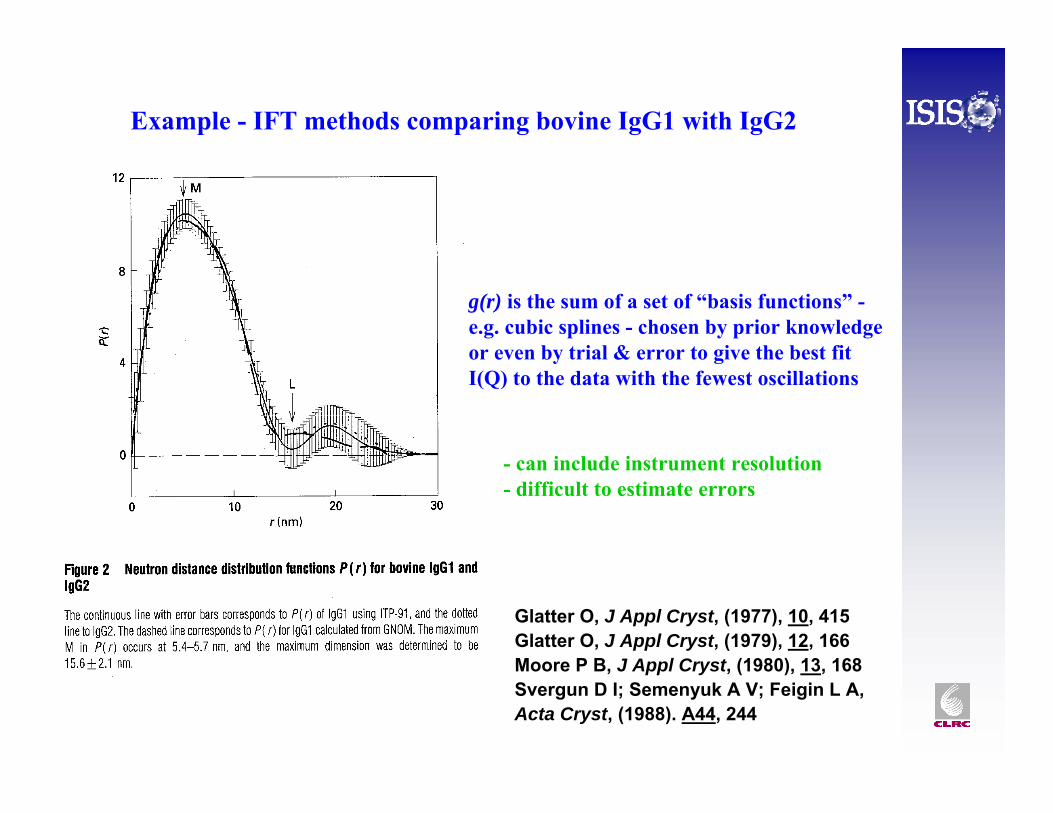
Example - IFT methods comparing bovine IgG1 with IgG2

g(r) is the sum of a set of “basis functions” -e.g. cubic splines - chosen by prior knowledge or even by trial & error to give the best fit I(Q) to the data with the fewest oscillations

- can include instrument resolution- difficult to estimate errors

Glatter O, J Appl Cryst, (1977), 10, 415Glatter O, J Appl Cryst, (1979), 12, 166Moore P B, J Appl Cryst, (1980), 13, 168Svergun D I; Semenyuk A V; Feigin L A, Acta Cryst, (1988). A44, 244

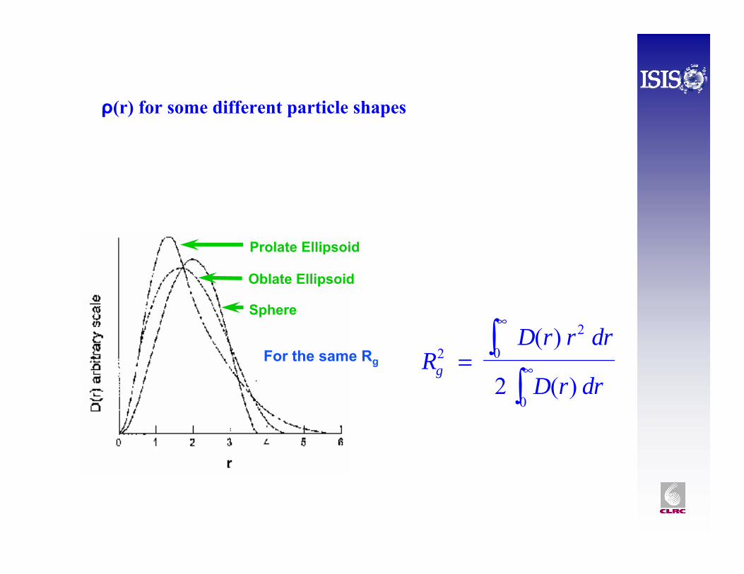
ρ(r) for some different particle shapes

RD r r dr

D r drg2

2

0

02

=

∞

∞∫∫

( )

( )

Sphere

Prolate Ellipsoid

Oblate Ellipsoid

For the same Rg

Computer Simulation Methods – usually for biomolecules

Can work very well for monodisperse biomolecules – all are the same size and shape – particularly if a number of different contrast are used to highlight parts of the structure (protein/DNA/carbohydrate etc) and if some parts have “known”structures from crystallography.

“Debye spheres modelling”

Simulated annealing (“dummy atom”) methods

See the web pages of Dimitri Svergun’s group at EMBL Hamburg:www.embl-hamburg.de/ExternalInfo/Research/Sax/index.html

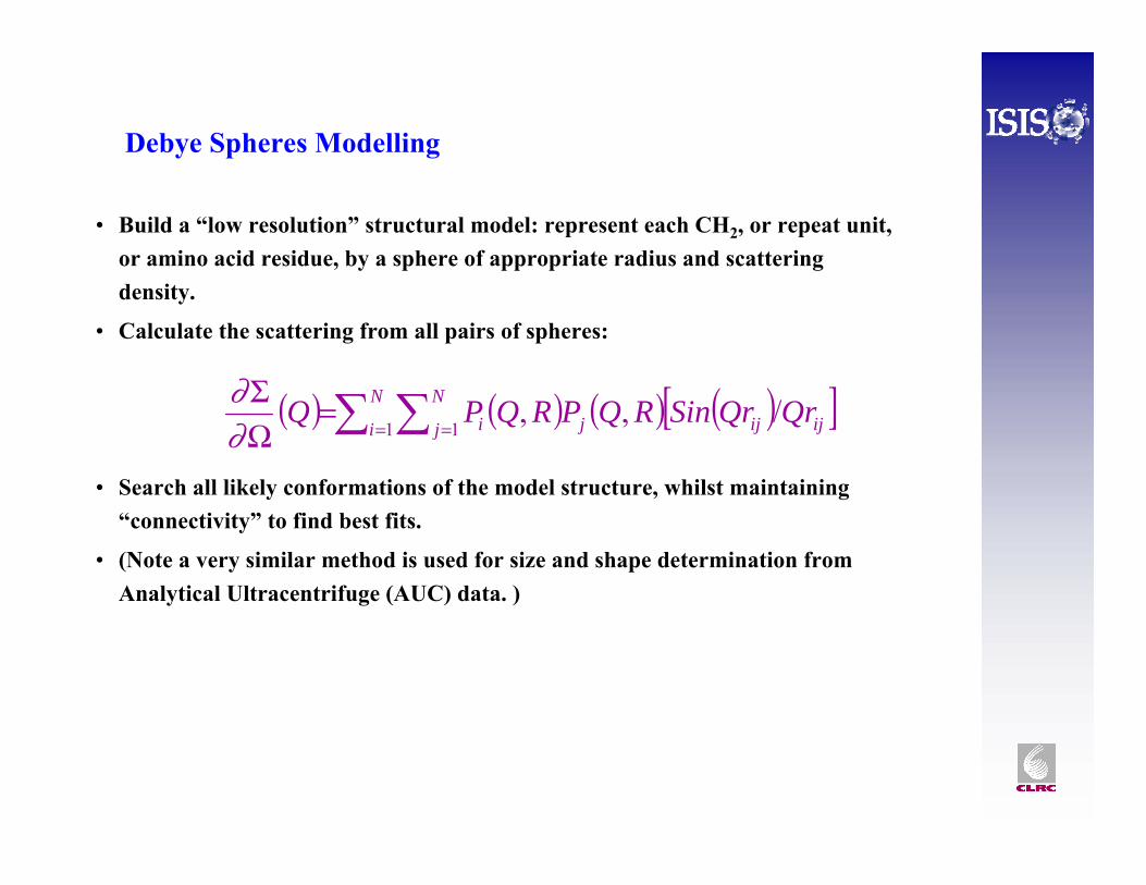
Debye Spheres Modelling

• Build a “low resolution” structural model: represent each CH2, or repeat unit, or amino acid residue, by a sphere of appropriate radius and scattering density.

• Calculate the scattering from all pairs of spheres:

• Search all likely conformations of the model structure, whilst maintaining “connectivity” to find best fits.

• (Note a very similar method is used for size and shape determination from Analytical Ultracentrifuge (AUC) data. )

( ) ( ) ( ) ( )[ ]ijijjN

i

N

j i QrQrSinRQPRQPQ /,,1 1∑ ∑= =

=ΩΣ

∂∂

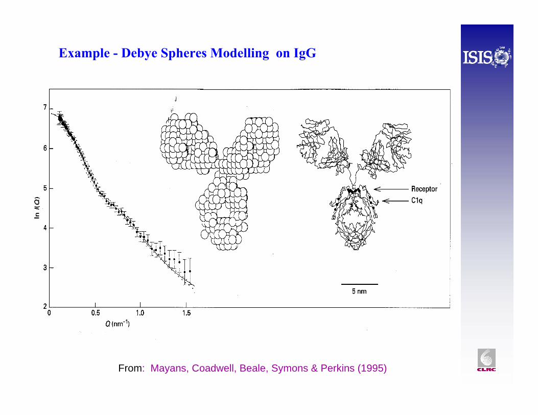
Example - Debye Spheres Modelling on IgG

From: Mayans, Coadwell, Beale, Symons & Perkins (1995)

The superposition of 104 best-fit molecular models (from 12000 conformations optimised by molecular dynamics, based on crystal structure coordinates) gives an idea of the solution conformation of human Immunoglobin IgA1

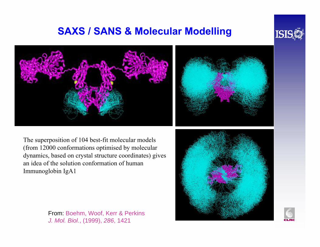
SAXS / SANS & Molecular Modelling

From: Boehm, Woof, Kerr & Perkins J. Mol. Biol., (1999), 286, 1421

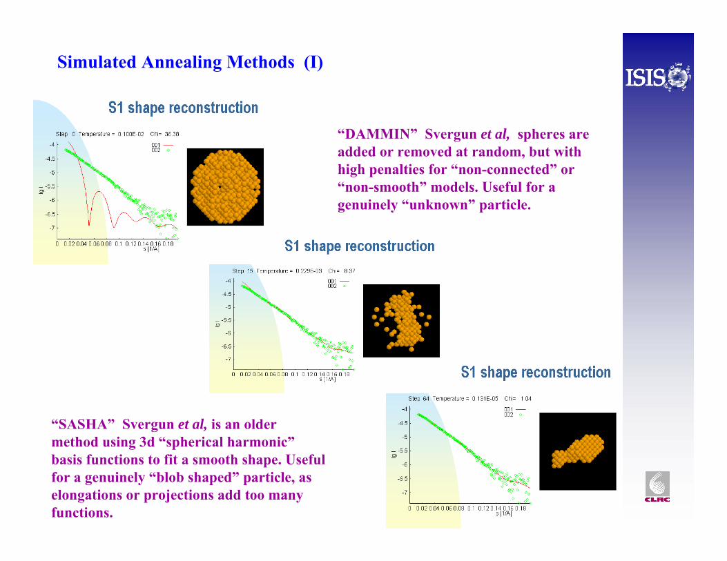
Simulated Annealing Methods (I)

“DAMMIN” Svergun et al, spheres are added or removed at random, but with high penalties for “non-connected” or “non-smooth” models. Useful for a genuinely “unknown” particle.

“SASHA” Svergun et al, is an older method using 3d “spherical harmonic”basis functions to fit a smooth shape. Useful for a genuinely “blob shaped” particle, as elongations or projections add too many functions.

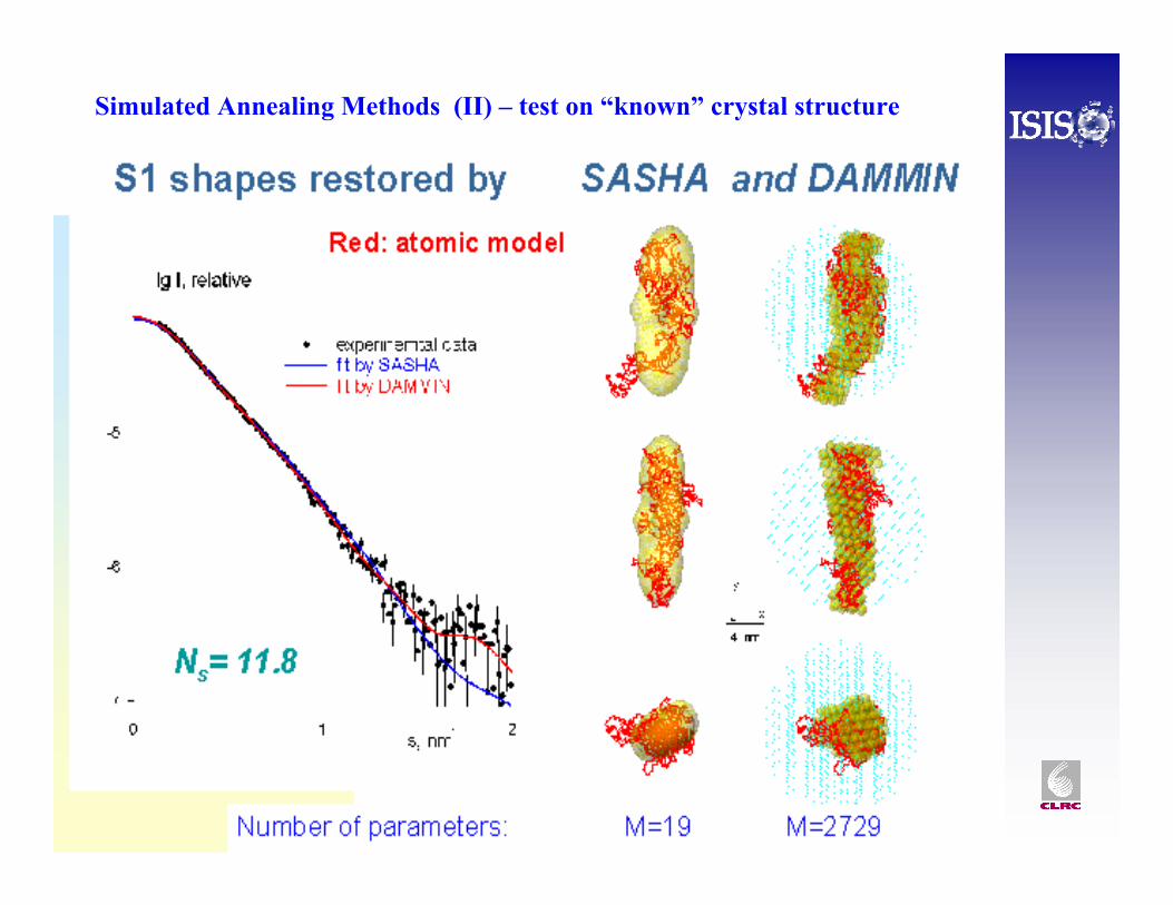
Simulated Annealing Methods (II) – test on “known” crystal structure

SANS on “biomolecules” – general comments

As we have seen, SAS can be very powerful for monodisperse (all the same size and shape) molecules.

Svergun’s group have a wide range of programs where more or less constraints, such as known crystal structures of fragments, may be included.

SANS is quite sensitive to any large aggregates due to the ΦV term in I(Q)

SANS can work at < 1mg/ml in most cases (but can be hard in H2O due to incoherent background from H).

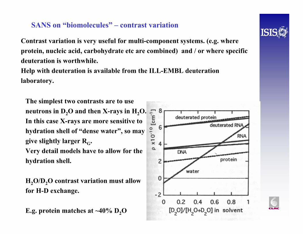
SANS on “biomolecules” – contrast variation

Contrast variation is very useful for multi-component systems. (e.g. where protein, nucleic acid, carbohydrate etc are combined) and / or where specific deuteration is worthwhile.Help with deuteration is available from the ILL-EMBL deuteration laboratory.

The simplest two contrasts are to use neutrons in D2O and then X-rays in H2O. In this case X-rays are more sensitive to hydration shell of “dense water”, so may give slightly larger RG.Very detail models have to allow for the hydration shell.

H2O/D2O contrast variation must allow for H-D exchange.

E.g. protein matches at ~40% D2O

Fibre Diffraction (I)

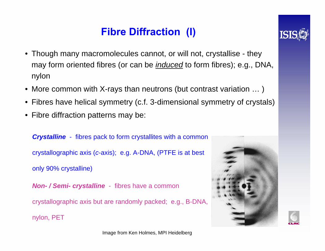
• Though many macromolecules cannot, or will not, crystallise - they may form oriented fibres (or can be induced to form fibres); e.g., DNA, nylon

• More common with X-rays than neutrons (but contrast variation … )

• Fibres have helical symmetry (c.f. 3-dimensional symmetry of crystals)

• Fibre diffraction patterns may be:

Crystalline - fibres pack to form crystallites with a common

crystallographic axis (c-axis); e.g. A-DNA, (PTFE is at best

only 90% crystalline)

Non- / Semi- crystalline - fibres have a common

crystallographic axis but are randomly packed; e.g., B-DNA,

nylon, PET

Image from Ken Holmes, MPI Heidelberg

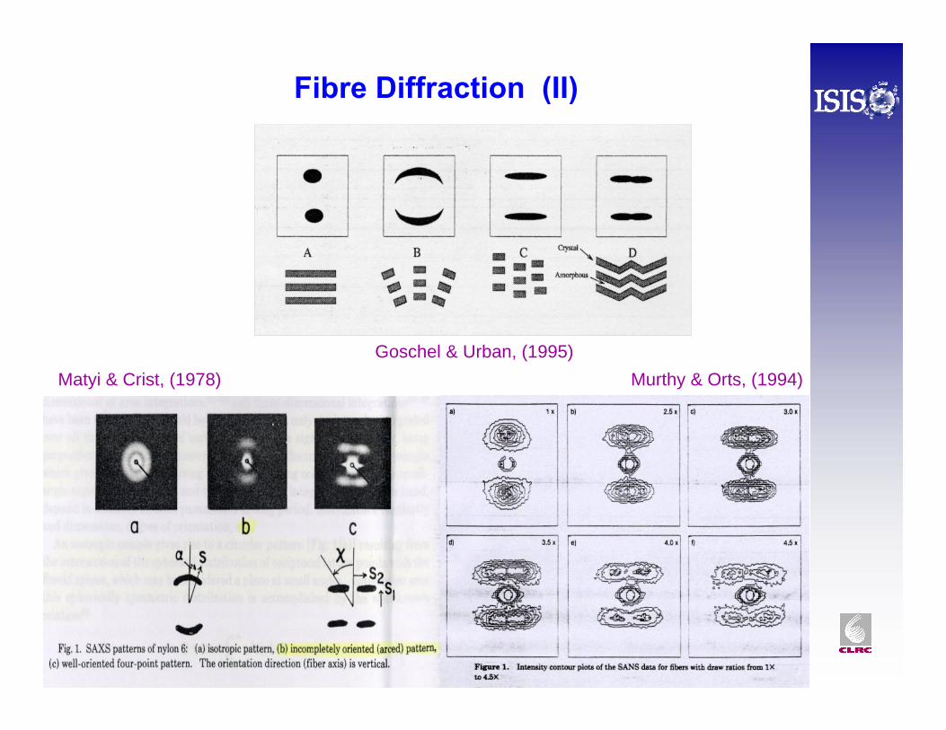
Fibre Diffraction (II)

Murthy & Orts, (1994)Matyi & Crist, (1978)Goschel & Urban, (1995)

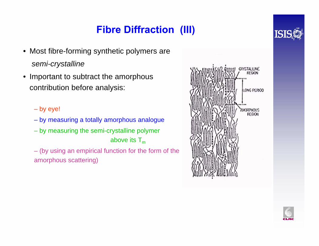
Fibre Diffraction (III)

• Most fibre-forming synthetic polymers are

semi-crystalline

• Important to subtract the amorphous contribution before analysis:

– by eye!

– by measuring a totally amorphous analogue

– by measuring the semi-crystalline polymer above its Tm

– (by using an empirical function for the form of the amorphous scattering)

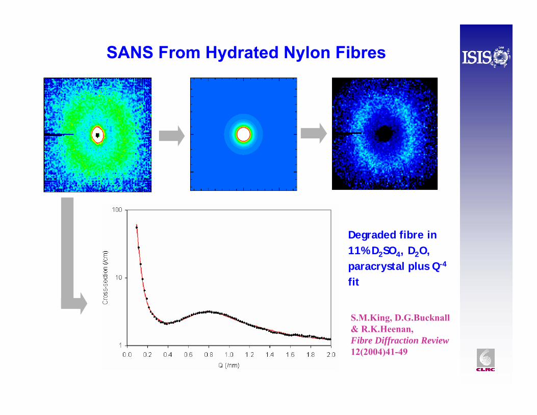
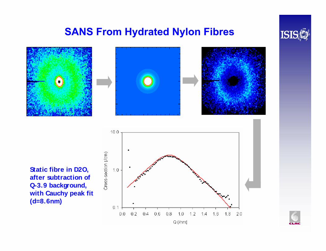
SANS From Hydrated Nylon Fibres

S.M.King, D.G.Bucknall& R.K.Heenan, Fibre Diffraction Review12(2004)41-49

Degraded fibre in 11% D2SO4, D2O, paracrystal plus Q-4

fit

SANS From Hydrated Nylon Fibres

Static fibre in D2O, after subtraction of Q-3.9 background, with Cauchy peak fit (d=8.6nm)

0.1

1.0

10.0

Cros

s-se

ctio

n (/

cm)

SANS From Hydrated Nylon Fibres

x Q2

Q*

Qd π2=

Peak width may give information about the distribution of d values.

(See Debye-Scherrerequation)

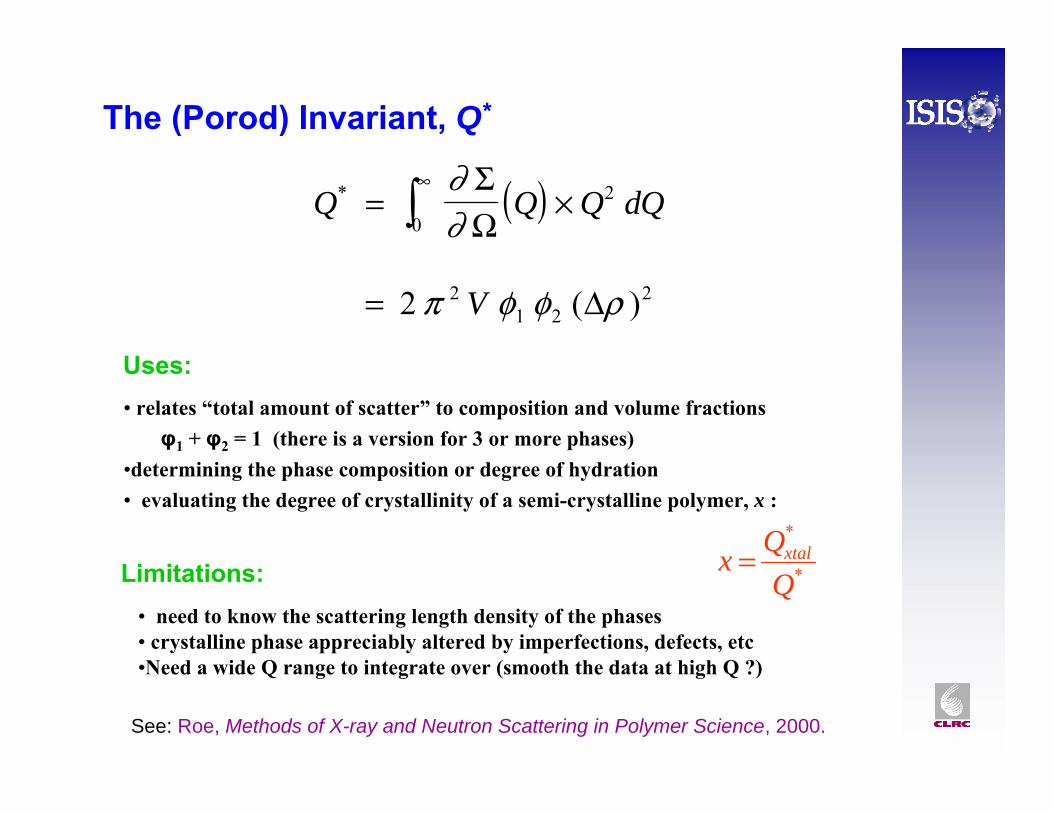
The (Porod) Invariant, Q*

( )Q Q Q dQ* = ×∞

∫∂∂

ΣΩ0

2

= 2 21 2

2π φ φ ρV ( )Δ

See: Roe, Methods of X-ray and Neutron Scattering in Polymer Science, 2000.

Uses:• relates “total amount of scatter” to composition and volume fractions

φ1 + φ2 = 1 (there is a version for 3 or more phases)•determining the phase composition or degree of hydration • evaluating the degree of crystallinity of a semi-crystalline polymer, x :

Limitations:• need to know the scattering length density of the phases• crystalline phase appreciably altered by imperfections, defects, etc•Need a wide Q range to integrate over (smooth the data at high Q ?)

*

*

QQx xtal=

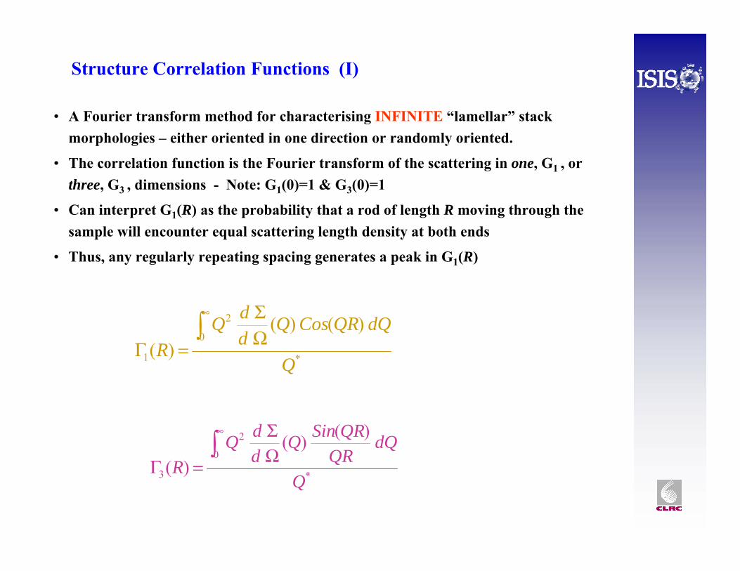
Structure Correlation Functions (I)

• A Fourier transform method for characterising INFINITE “lamellar” stack morphologies – either oriented in one direction or randomly oriented.

• The correlation function is the Fourier transform of the scattering in one, G1 , or three, G3 , dimensions - Note: G1(0)=1 & G3(0)=1

• Can interpret G1(R) as the probability that a rod of length R moving through the sample will encounter equal scattering length density at both ends

• Thus, any regularly repeating spacing generates a peak in G1(R)

*

0

2

1

)()()(

Q

dQQRCosQddQ

R∫

∞

ΩΣ

=Γ

*

0

2

3

)()()(

Q

dQQR

QRSinQddQ

R∫

∞

ΩΣ

=Γ

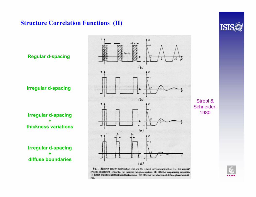
Regular d-spacing

Irregular d-spacing

Irregular d-spacing+

thickness variations

Irregular d-spacing+

diffuse boundaries

Strobl & Schneider,

1980

Structure Correlation Functions (II)

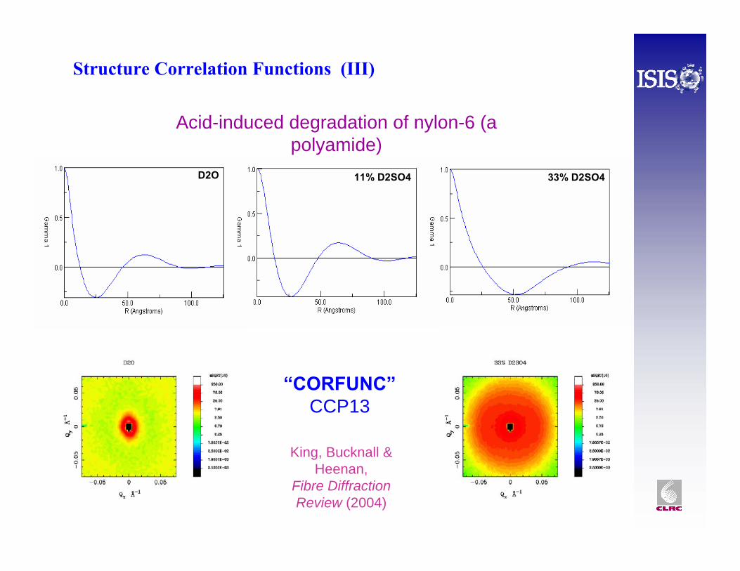
D2O 11% D2SO4 33% D2SO4

Acid-induced degradation of nylon-6 (a polyamide)

“CORFUNC”CCP13

King, Bucknall & Heenan,

Fibre Diffraction Review (2004)

Structure Correlation Functions (III)

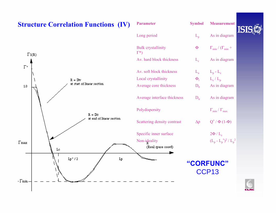
Correlation Functions

“CORFUNC”CCP13

Parameter Symbol Measurement

Long period Lp As in diagram

Bulk crystallinity Φ Γmin / (Γmin + Γ*)

Av. hard block thickness Lc As in diagram

Av. soft block thickness La Lp - Lc

Local crystallinity Φl Lc / Lp

Average core thickness D0 As in diagram

Average interface thickness Dtr As in diagram

Polydispersity Γmin / Γmax

Scattering density contrast Δρ Q* / Φ (1-Φ)

Specific inner surface 2Φ / Lc

Non-ideality (Lp - Lp*)2 / Lp

2

Structure Correlation Functions (IV)

CCP13CCP13 is the Collaborative Computational Project for Fibre and (latterly) Polymer Diffraction established on 1st January 1992. It is supported by the BBSRC and EPSRC.

CCP13 exists to focus the development of software for the analysis of data from a variety of samples exhibiting order and/or preferential alignment.

The CCP13 program suite is free.

The programs run under a number of Unix operating systems including Linux. Severalprograms also run under Windows NT/2000/XP.

Programs:• File conversion utilities

• Preliminary analysis of fibre diffraction patterns• Integration of fibre diffraction pattern intensities• Fourier-Bessel smoothing of layer lines

• Image space to reciprocal space transformation

• Peak fitting• Correlation function analysis

http://www.ccp13.ac.uk

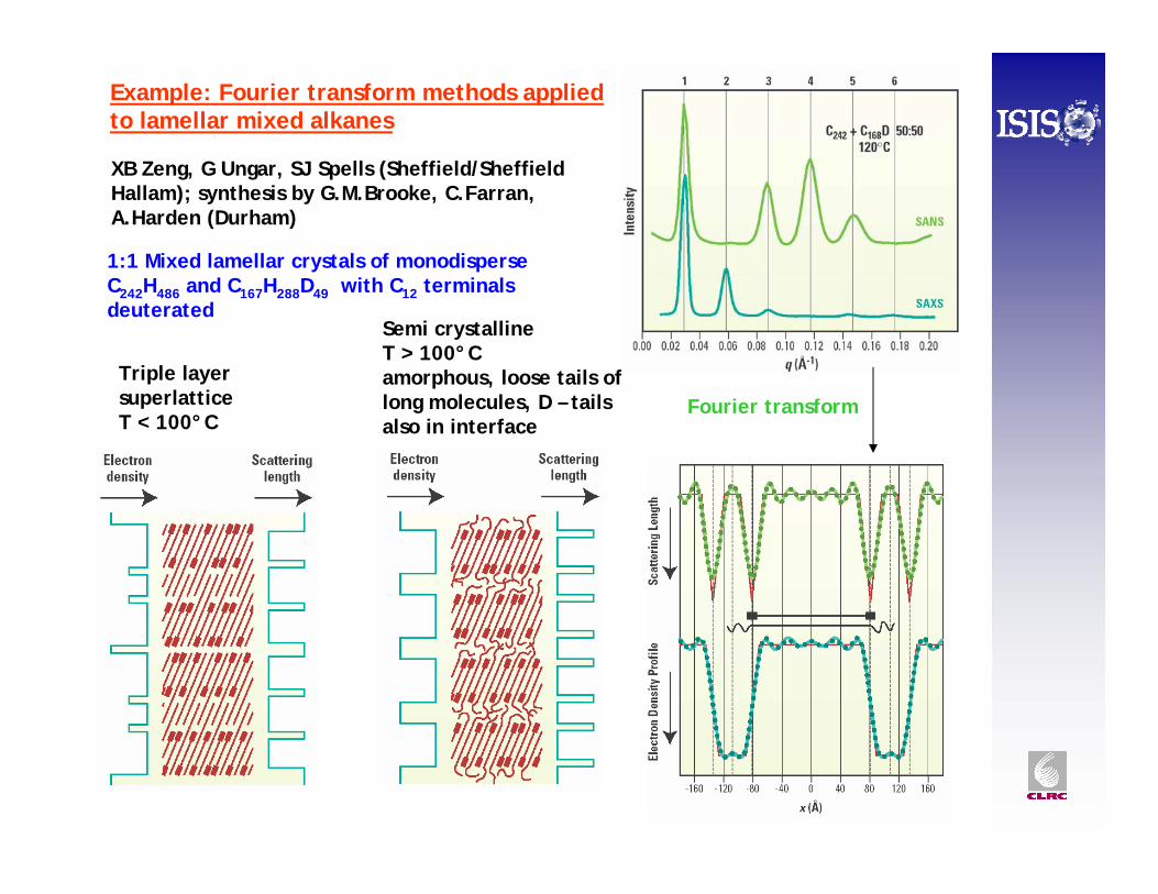
XB Zeng, G Ungar, SJ Spells (Sheffield/Sheffield Hallam); synthesis by G.M.Brooke, C.Farran, A.Harden (Durham)

1:1 Mixed lamellar crystals of monodisperseC242H486 and C167H288D49 with C12 terminals deuterated

Semi crystalline T > 100°Camorphous, loose tails of long molecules, D – tails also in interface

Triple layer superlatticeT < 100°C

Fourier transform

Example: Fourier transform methods applied to lamellar mixed alkanes

0

20

40

60

0.00 0.05 0.10 0.15

q (1/Å)

I(q)

NIF Folded-Extended

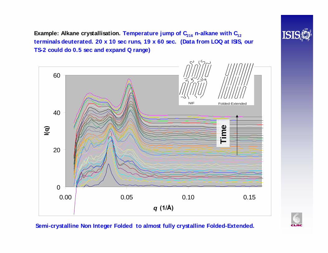
Example: Alkane crystallisation. Temperature jump of C216 n-alkane with C12

terminals deuterated. 20 x 10 sec runs, 19 x 60 sec. (Data from LOQ at ISIS, our TS-2 could do 0.5 sec and expand Q range)

Semi-crystalline Non Integer Folded to almost fully crystalline Folded-Extended. Ti

me