Singularity structure of the πN scattering amplitude in a meson-exchange model up toenergies W ≤ 2.0 GeV

L. Tiatora, S.S. Kamalova,b,d, S. Cecic, Guan Yeu Chend, D. Drechsela, A. Svarcc, and Shin Nan Yangd

aInstitut fur Kernphyik, Universitat Mainz, D-55099 Mainz, GermanybBogoliubov Laboratory for Theoretical Physics, JINR, Dubna, 141980 Moscow Region, Russia

cRudjer Boskovic Institute, Division of Experimental Physics, HR-10002 Zagreb, CroatiadDepartment of Physics and Center for Theoretical Sciences, National Taiwan University, Taipei 10617, Taiwan

(Dated: October 11, 2010)

Within the previously developed Dubna-Mainz-Taipei meson-exchange model, the singularitystructure of the πN scattering amplitudes has been investigated. For all partial waves up to F wavesand c.m. energies up to W ∼ 2 GeV, the T -matrix poles have been calculated by three differenttechniques: analytic continuation into the complex energy plane, speed-plot, and regularizationmethod. For all 4-star resonances except the S11(1535), we find very good agreement between theanalytic continuation and the regularization method. We also find resonance poles for resonancesthat are not so well established, but in these cases the pole positions and residues obtained byanalytic continuation can substantially differ from the results predicted by the speed-plot andregularization methods.

PACS numbers: 11.80.Gw, 13.75.Gx, 14.20.Gk, 25.80.DjKeywords: pion-nucleon interaction, baryon resonances, T-matrix poles, speed plot, regularization method

I. INTRODUCTION

Ever since the ∆(1232) resonance was discovered by Fermi and collaborators in 1952 [1–3], the excitation spectrum

of the nucleon has played a fundamental role in our understanding of low-energy hadronic physics. The most direct

evidence for resonance structure is based on pion-nucleon elastic and charge-exchange scattering. Because total

angular momentum, parity, and isospin are conserved within the realm of the strong interaction, the S matrix for

the reactions π + N → π′ + N ′ may be decomposed into the partial wave amplitudes T I`±, with I the isospin,

` the orbital angular momentum, and the ± indicating the total spin of the hadronic system, J = ` ± 12 . Two

decades after the discovery of the ∆(1232), a dedicated program at the meson factories had provided enough data to

establish a rich resonance spectrum of the nucleon [4, 5]. The further partial wave analysis was driven by studies

of the Karlsruhe-Helsinki (KH) [6, 7] and Carnegie-Mellon–Berkeley (CMB) [8, 9] collaborations. In the following

years, R. Arndt and coworkers at VPI compiled the data base SAID [10], which was later updated and extended in

collaboration with GWU [11, 12]. The works of the CMB, KH, and GW/VPI groups are the main sources of the

nucleon resonance listings in the Review of Particle Physics (PDG) [13].

In the most intuitive way, a resonance is an intermediate state of target and projectile that lives longer than

in a typical scattering process. Translated into the language of scattering theory, resonances are defined as poles

of the S matrix. Different methods were developed to derive the resonance properties from the observables.

In the 1930’s it was suggested that a Breit-Wigner function should be a good representation for a resonance

pole, and the Breit-Wigner formula for spin zero particles and its generalization to finite spin were developed

(see an illustrative discussion in Cottingham and Greenwood, p. 241 in Ref. [14]). Later the discussion centered

on the rapid increase of the eigenphase shifts through 90◦ and on the related backward looping of Argand diagrams [15].

2

However, Breit-Wigner parametrizations have been found to be very model dependent. As was recently shown in the

framework of effective quantum field theory, Breit-Wigner masses are in general field-redefinition dependent [16]. The

same model dependency also applies to electromagnetic properties as charges, magnetic moments, transition moments,

and form factors. On the other side, all these resonance properties are uniquely defined at the pole of the S matrix [17].

The analytic properties of the S matrix are imposed by the principles of unitarity and causality. Because of

unitarity, each physical channel leads to a square-root type branch point of the partial wave amplitude T (W ) at the

respective threshold, with the result that T (W ) is a multi-valued function in the complex W plane. In particular,

if the branch cut is taken on the real axis to the right, a partial wave for elastic πN scattering is described by the

amplitudes T [1] on the physical and T [2] on the unphysical sheet. The experimental amplitudes are identified with

the amplitudes above the cut, Texp(W ) = limε→0 T [1](W + i ε), with W > M + m and ε > 0. As a consequence, the

physical sheet has a discontinuity over the real axis, along the right-hand cut M + m ≤ W < ∞, with M the nucleon

and m the pion mass. Causality requires that the physical sheet be free of any further singularity, the nucleon

resonances should appear as simple poles on the unphysical sheet closest to the real axis of the physical sheet, in

agreement with Hohler’s remark [18]: “It is ‘noncontroversial among theorists’ (see Chew [19] and the references in

my ‘pole-emics’, p.697 in Ref. [20]) that in S-matrix theory the effects of resonances follow from first order poles

in the 2nd sheet.” A pole on the second sheet, described by T [2](W ) ≈ rp/(Mp −W − i Γp/2), will often lead to a

maximum of the experimental cross section near W = Mp. The resonance is therefore defined by (i) its pole position

in the complex c.m. energy plane at Wp = Mp − i Γp/2, with Mp the real part of the pole position and Γp the width

of the resonance, and (ii) the residue of the amplitude, rp = |rp|exp(i θp), at the pole.

In a more physical way, resonance is characterized by a maximum time delay, the time passing between the arrival

of a wave packet and its departure from the collision region. In general, a large time delay indicates the formation

of an unstable particle in the intermediate state. However, misleading effects can occur by rapid variation of

backgrounds, such as narrow cusp effects above S-wave thresholds or spurious singularities due to phenomenological

parametrization of form factors and cut-offs. If a resonance lives long enough, it should decay into all energetically

possible final states, unless prevented by general selection rules. Furthermore, the pole position derived from the

data should not depend on how the resonance is excited or decays. Whereas such resonances exist in atomic and also

in nuclear physics, some caveat is in order for nucleon resonances. As an example, a simple classical model of the

∆(1232) leads to the conclusion that the pion stays in its orbit around the nucleon for only about 100◦ of a full circle.

The focus of the present work is on how to extract resonance properties from the data, that is, how do we find a

pole in the complex energy plane having at our disposal only data on the real axis. Different pole-extraction methods

have been applied in the past. The pole positions of nucleon resonances have often been derived from the data by

the speed plot [4, 21], which is related to the time delay. The “speed” is defined by the slope of the amplitude

with energy, dT (W )/dW , which eliminates constant backgrounds. The “speed plot” (SP) shows the modulus of the

speed, SP(W ) = |dT (W )/dW |, and resonances are identified with peaks in the plot. The resonance parameters are

then obtained by fitting the speed of a single pole to the data at physical values of the energy. The idea of the

speed plot has been recently generalized to higher derivatives by the “regularization method” (RM) [22]. Within

a convergence circle given by the closest neighboring singularity, the Laurent expansion about a pole is given by

the sum of T pole(W ) and a Taylor series T reg(W ). With an increasing number of differentiations, the signature of

the pole sticks out more and more sharply, whereas more and more leading terms of the Taylor series disappear. It

3

goes without saying that the differentiation of the data will fail after a few steps because of numerical instabilities.

However, the regularization method is an interesting tool to study the singularity structure of analytic models. In

particular, this method will reveal any rapid variation due to cusp effects and spurious singularities introduced by

phenomenological parameterizations.

Although Lattice QCD (LQCD) has obtained promising results for the masses and several resonances of the

low-lying hadrons [23–25], the large pion mass used and the quenching approximation make it (yet) impossible to

treat the resonances as a pion-nucleon scattering state. As shown by Ref. [26] for the N∆ form factors, the chiral

extrapolation from the stable ∆ at large pion masses to the experimental pion mass yields unexpected and rather

dramatic non-analytic effects at the ∆ → Nπ threshold. The very fact that lattice theory can not yet describe the

pion-nucleon final state interaction, makes it impossible to compare the lattice data to the experimental scattering

amplitudes in a direct way. In principle, the LQCD data should be compared to the results of effective field theories

or dynamical models which are extrapolated to the pion mass used in LQCD. In addition to kinematical mass effects

such as shifts of branch points also the mass dependence of the coupling constants should be considered. As long as

the pion mass is large, mπ > mN∗ −mN , the N* appears as an excited bound state. In this case the mass predicted

by LQCD should be compared to the ”dressed” mass of the dynamical model, which contains the ”bare” mass

and a real self-energy due to meson loops. In the mass region where the N* decays, the LQCD calculation would

provide a complex amplitude, comparable to the scattering phases of a partial wave expansion. Based on the work

of Luscher [27], the width of the rho meson [28] and of the Delta resonance [29] have been recently studied. In such

a case the lattice data can be treated like experimental amplitudes, that is, by speed plot or Breit-Wigner analyses.

However, as long as the LQCD pion mass lies above the physical value, an extrapolation to the physical pion mass

will still be necessary by use of a dynamical model or an effective field theory.

In the present contribution we study the Dubna-Mainz-Taipei model (DMT) [30] by comparing the pole parameters

resulting from analytic continuation with approximate procedures such as the speed plot and the regularization

method. The DMT is similar in spirit with the work of several other collaborations [30–36] who have studied the

nucleon resonances within Lagrangian models. The building blocks of these models are “bare” resonances simulating

quark configurations which are “dressed” by meson-nucleon continua through the respective Lagrangians. Compared

to the partial wave amplitudes obtained in Refs. [8–12], the dynamical models provide a field-theoretical description

of pion-nucleon scattering by meson-baryon loops. Therefore, the energy dependence of the DMT amplitudes is

largely determined by theoretical considerations even though there are free parameters in the model. Another

strong point of the DMT is the fact that its predictions for electromagnetic pion production [37–39] are in excellent

agreement with the experimental data from threshold up to the ∆(1232) region. In Sect. II we give an overview

of the speed-plot, time-delay, and regularization methods to derive the pole parameters. The Dubna-Mainz-Taipei

model is presented in Sect. III, in particular with regard to the definitions of resonant vs. background terms as well

as form factors and cut-offs. Our results for the resonance parameters are reported in Sect. IV, and the different

techniques to derive these parameters are compared. We conclude with a summary and outlook in Sect. V.

4

II. HOW TO FIND A RESONANCE

A. Time delay

In the framework of a potential scattering problem, resonance phenomena are related to the formation and the

decay of intermediate quasi-stationary states. A resonance should decay in all energetically possible final states,

unless forbidden by selection rules for a specific channel. Provided that the interaction is of short range, resonances

can be characterized by the time delay between the arrival of a wave packet and its departure from the collision

region. In general, the time delay shows a pronounced peak at the resonance energies. The time delay was introduced

by Eisenbud in his Ph.D. thesis [40] and later applied to multi-channel scattering theory by Smith [41]. Following the

work of Refs. [15, 42–44], we define the time delay for a single-channel scattering problem in a partial wave as follows:

∆t(W ) = Re(−i

1S(W )

dS(W )dW

)= 2

dδ(W )dW

, (1)

where S(W ) = exp[2iδ(W )] is the S matrix and δ(W ) the scattering phase shift. A simple ansatz for a unitary S

matrix with a pole at Wp = Mp − i2Γp and a constant background phase δB is given by

S(W ) =Mp + i

2Γp −W

Mp − i2Γp −W

e2iδB = e2iδR(W ) e2iδB , (2)

where δR(W ) = arctan[ 12Γp/(Mp −W )] is the resonant phase. The related T -matrix T = (S − 1)/(2 i) and the real

matrix K = i (1− S)(1 + S)−1 take the forms

T (W ) =12Γp

Mp − i2Γp −W

e2iδB + sinδBeiδB , (3)

K(W ) =12Γp + (Mp −W )tanδB

Mp −W − 12ΓptanδB

. (4)

Combining Eqs. (1) and (2), we obtain a simple form for the time delay,

∆t(W ) =Γp

(W −Mp)2 + 14Γ2

p

. (5)

In this ideal case, the maximum time delay is ∆t(Mp) = 4/Γp. We observe that both the real (Mp) and imaginary

(− 12Γp) parts of the pole position are determined by the time delay (and therefore also by the scattering matrix) at

real (physical!) values of the c.m. energy W .

In order to describe a system of coupled channels, the lifetime matrix Q was introduced [41],

Qij(W ) = −idSik(W )

dWS∗jk(W ) . (6)

The analog of the time delay for a multi-channel system was found to be the trace of Q as function of W . This trace

takes a more transparent form after diagonalization of the S matrix [15, 45],

tr[Q(W )] = 2∑α

dδα(W )dW

, (7)

with δα the eigenphase shifts. However, a realistic application of the lifetime matrix requires the knowledge of all

open channels, that is, the reactions πN → πN , πN → ππN , ππN → ππN , πN → ηN , and so on. As a consequence

of the Neumann-Wigner no-crossing theorem [46], individual eigenphases have a complicated energy dependence. It

5

is therefore only the sum of the eigenphases that shows distinct resonance structures. Based on this observation,

it has been recently proposed to search for resonance parameters by studying the traces of multi-channel T and K

matrices [47, 48]. The respective scattering matrices were constructed from experimental data for the πN and ηN

channels and models for the two-pion channels.

B. Speed plot

The speed plot of a partial wave amplitude T is defined by

SP(W ) =∣∣∣∣dT (W )

dW

∣∣∣∣ . (8)

As was recognized by the Particle Data Group already in the early 1970’s, the speed plot is a convenient tool to

extract the pole position of a resonance [5, 49]. This technique was intensively studied by Hohler who wanted to

extract resonance parameters from the Karlsruhe-Helsinki partial wave analysis (KH80) [21, 50]. Because the KH

analysis was restricted to elastic pion-nucleon scattering, a multi-channel treatment like the construction of the

lifetime matrix was out of reach.

For a single channel system, the time delay and the speed plot are identical up to a factor 2. In particular, the pole

ansatz of Eq. (3) leads to the speed

SP(W ) =12Γp

(W −Mp)2 + 14Γ2

p

. (9)

As a result, the speed plot shows a maximum for W = Mp, which defines the real part of the pole position in the

complex W plane. The imaginary part of the pole position can be obtained from the relation

SP(Mp ± 12Γp) = 1

2 SP(Mp) . (10)

In practical applications, this straightforward method has to be modified. In the vicinity of a pole, Eq. (3) can be

generalized to

T (W ) =rp

Mp −W − i2 Γp

+ T reg(W ) (11)

with T reg a regular function of the energy W and rp, the complex residue at the pole, given by

Res T (W )|W=Wp= − | rp | eiθp . (12)

If all higher-order terms are neglected, Eq. (8) leads to the more general speed

SP(W ) =|rp|

(W −Mp)2 + 14Γ2

p

, (13)

which is fitted to speed data obtained from the partial wave amplitudes in the vicinity of the maximum. The pole

parameters Mp,Γp and |rp| are then obtained from the best fit to the selected speed points. Finally, the phase θp of

the residue is obtained from the phase of dT/dW ,

θp = arg

(− dT

dW

∣∣∣∣W=Mp

). (14)

6

C. Regularization method

As discussed before, the speed plot technique is successful if the background under the resonance is approximately

constant. It fails if the background changes over the resonance region. The regularization method extends the idea

behind the speed plot by construction of higher derivatives, T (N) ≡ dN T/dTN , N ≥ 1 [22]. Let there be an analytic

function T (z) of a complex variable z with a first-order pole at some complex point µ = x + iy. This function can be

any of the T -matrix elements, and the variable z is identified with the c.m. energy W in order to compare with the

speed plot technique. The described function takes the form

T (z) =r

µ− z︸ ︷︷ ︸pole part

+(

T (z)− r

µ− z

)

︸ ︷︷ ︸non−pole part

, (15)

where µ and r are the position and residue of the pole. In a sufficiently small region around the pole, the non-pole part

is a smooth analytical function. Of course, the experiment can determine the T -matrix elements only for real values

of W . In order to continue T (W ) into the complex energy plane and to search for the pole position, we construct a

regular function f by multiplying T with the factor µ− z,

f(z) = (µ− z) T (z) , (16)

with f(µ) = r. In the neighborhood of the pole, the function f can be expanded in a Taylor series. Because the

scattering matrix can be accessed for real arguments only, we construct f(µ) from the derivatives of f taken along

the real axis,

r = f(µ) =N∑

n=0

f (n)(W )n!

(µ−W )n + RN (W,µ). (17)

This expansion is explicitly written to order N , and RN (W,µ) stands for the higher orders. The derivatives f (n)(W )

can be turned in derivatives of the T matrix by use of Eq. (16), and mathematical induction leads to the following

equation:

f (n)(W ) = (µ−W )T (n)(W )− n T (n−1)(W ). (18)

Insertion of these derivatives into Eq. (16) cancels all the terms in the sum except for the last one,

r =T (N)(W )

N !(µ−W )(N+1) + RN (W,µ) . (19)

In the neighborhood of the pole, the remainder RN should decrease with increasing N . Assuming that the higher

derivatives can be neglected for a sufficiently large value of N and taking the absolute values of both sides, we obtain

an approximation of the pole parameters at O(N),

|rN | =∣∣T (N)(W )

∣∣N !

|µN −W |(N+1). (20)

On condition that the Taylor series converges and in the limit N → ∞, rN and µN should approach the values r

and µ, respectively. In the next step, we (i) write the pole position as a general complex number, µ = a + i b, (ii)

raise both sides of Eq. (20) to the power of 2/(N + 1), and collect the information about the T -matrix and the pole

position on the right and left side, respectively. The result is a parabolic equation in W ,

(aN −W )2 + b2N

N+1√|rN |2

= N+1

√√√√ (N !)2∣∣T (N)(W )∣∣2 . (21)

7

This equation relates the pole position (a = Mp, b = − 12 Γp) and the absolute value of the residue, |r|, to the T-matrix

values on the real axis, as obtained from a model or an energy-dependent partial-wave analysis of the data. Finally,

the phase of the residue is determined by

θN = arg(

(−i)N+1 T (N)(Mp))

. (22)

The comparison of the above equations with the results of Sect. II B shows that the speed plot is identical to the

regularization method for N = 1.

The further procedure is as follows: (i) Construct the N th derivative of the T -matrix element and the right-hand

side of Eq. (21). Note that the pole parameters are uniquely determined by the exact knowledge of T (W ) in only

three points. However, the problem is to choose the right points. If the distance between the points gets too large,

the influence of other singularities may increase. If the points are too close, numerical problems may occur. (ii)

Solve Eq. (21) for the pole parameters by either choosing various three-point sets to evaluate the right-hand side and

perform a statistic analysis of the results or fitting the right-hand side of the equation to a three-parameter parabolic

function. In our approach we have chosen the latter option.

In closing this section we note that the regularization method does not depend on any particular functional form of

the T matrix. However, we have to assume that (a) the N th derivative can be constructed with a sufficient precision

and (b) the pole position lies within the circle of convergence for the Taylor expansion, that is, no further singularities

should intrude into the region between the pole and the related resonance region on the real W axis.

D. Poles from analytic continuation

The most accurate way to determine pole positions and residues is certainly obtained by analytic continuation into

the complex region. Because resonance poles can not appear on the physical sheet, we have to take a careful look at

the structure of different Riemann sheets opening at all branch points for particle production in a coupled-channels

model. The most important particle thresholds in our energy region below 2 GeV are ππN , π∆, ηN , and ρN with

branch points at 1178 MeV, (1350− 50i) MeV, 1486 MeV, and (1713− 75i) MeV, in order. In the dynamical DMT

model we have included the πN and ππN channels in all the partial waves and the ηN channel in the S11 partial

wave. However, the ππN channel is treated in a phenomenological way as will be described in the following section.

Because the particular ansatz for the two-pion width, Eq. (36), contains only even powers of q2π, the model does not

give additional branch points for the two-pion channel. This leads to a relatively simple sheet structure, and we can

easily reach the poles on the most important second Riemann sheet (first unphysical sheet). Technically, we first map

the relevant region on this sheet by contour plots and search for the accurate pole position by standard root finding

routines applied to the function

h(zp) =1

|T (zp)| = 0 . (23)

Next we obtain the residue by approaching the pole along different paths in the complex plane,

ResT (z)|zp= lim

z→zp

(z − zp) T (z) . (24)

A word of caution is in order. If the fitted form factor parameters, e.g., Λα of Eq. (32) or XR of Eq. (36) become

smaller than about 500 MeV, additional poles can appear in the region where the resonance poles are expected. In

8

order to avoid such spurious singularities, it is very important to map out the structure of the T matrix very precisely.

Also the speed-plot and regularization methods are very helpful to distinguish between resonance and spurious poles,

because the latter ones usually affect the T matrix at real W in a similar way as a broad background does.

III. THE DUBNA-MAINZ-TAIPEI MESON-EXCHANGE MODEL

The Dubna-Mainz-Taipei (DMT) πN meson-exchange model was developed on the basis of the Taipei-Argonne

πN meson-exchange model [51–53] which describes pion-nucleon scattering up to 400 MeV pion laboratory energy.

The DMT πN model was extended to c.m. energies W = 2.0 GeV by inclusion of higher resonances and the ηN

channel [30, 54]. The model describes well both πN phase shifts and inelasticity parameters in all the channels up

to the F waves and energies of 2 GeV [55], except for the F17 partial wave. The DMT πN model is also a main

ingredient of the DMT dynamical model describing the photo- and electroproduction of pions [56] up to 2 GeV. This

model gives an excellent agreement with pion production data from threshold to the first resonance region [37, 57].

In this section, we briefly outline the ingredients of the Taipei-Argonne πN model and then describe some relevant

features of the DMT meson-exchange coupled-channels model. For more details, we refer readers to [30, 53, 54].

A. Taipei-Argonne meson-exchange πN model

The Taipei-Argonne model describes the elastic scattering of pions and nucleons. It is based on a three-dimensional

reduction of the Bethe-Salpeter equation for an effective Lagrangian involving π, N , ∆, ρ, and σ fields. Let us consider

the πN scattering,

π(q) + N(p) → π(q′) + N(p′) , (25)

where q, p, q′, and p′ are the four-momenta of the respective particles. The total and relative four-momenta are

P = p + q and k = p ηπ(s)− q ηN (s), respectively, where s = P 2 = W 2. The dimensionless variables ηπ(s) and ηN (s)

represent a freedom in choosing a three-dimensional reduction, and are constrained by ηN + ηπ = 1.

The Bethe-Salpeter equation for πN scattering takes the form

TπN = BπN + BπNG0TπN , (26)

where BπN is the sum of all irreducible two-particle Feynman amplitudes and G0 the free relativistic πN propagator.

Eq. (26) can be cast into the form

TπN = BπN + BπN G0TπN , (27)

with

BπN = BπN + BπN (G0 − G0)BπN , (28)

where G0(k; P ) is an appropriate propagator to obtain a three-dimensional reduction of Eq. (26). This propagator is

typically chosen to maintain the two-body unitarity by reproducing the πN elastic cut. However, there is still a wide

range of possible propagators satisfying this constraint. We chose the Cooper-Jennings propagator [58] since it can

satisfy the soft-pion theorems. It takes the following form in the c.m. frame:

G0(k; s) =1

(2π)3δ[k0 − η(s~k,~k)]√

s−√s~k

2√s~k√s +√

s~k

f(s, s~k)ηN (s)γ0

√s + k/ + mN

4EN (~k)Eπ(~k), (29)

9

where EN (~k) and Eπ(~k) are the nucleon and pion energies for three-momentum ~k; √s~k = EN (~k) + Eπ(~k) is the total

c.m. energy, and η(s,~k) = EN (~k)− ηN (s~k)√s~k , with ηN (s) = (s + m2N −m2

π)/2s. With these relations we obtain the

following πN scattering equation:

t(~k′,~k; W ) = v(~k′,~k;W ) +∫

d ~k′′v(~k′, ~k′′; W )g0(~k′′; W )t( ~k′′,~k;W ) , (30)

where t and v are related to T (k′, k; P ) and B(k′, k; P ) by setting k′0 = η(s~k′ ,~k′) and k0 = η(s~k,~k), while g is obtained

from G with k0 = 0.

The effective Lagrangian involving the π,N, σ, ρ, and ∆(1232) fields takes the form

LI =f

(0)πNN

mπNγ5γµ~τ · ∂µ~πN − g(s)

σππmπσ(~π · ~π)− g(v)σππ

2mπσ(∂µ~π · ∂µ~π)− gσNN NσN

−gρNN N{γµ~ρ µ +κρ

V

4mNσµν(∂µ~ρ ν − ∂ν~ρ µ)} · 1

2~τN

−gρππ~ρ µ · (~π × ∂µ~π)− gρππ

4m2ρ

(δ − 1)(∂µ~ρ ν − ∂ν~ρ µ) · (∂µ~π × ∂ν~π)

+gπN∆

mπ∆µ[gµν − (Z +

12)γµγν ]~T∆NN · ∂ν~π , (31)

with ∆µ the ∆ field operator and ~T∆N the isospin transition operator between nucleon and ∆. The pseudovector

πNN coupling is dictated by the chiral symmetry.

The driving term BπN in Eq. (26) is approximated by the tree diagrams of the interaction Lagrangian of Eq. (31),

containing direct and crossed N and ∆ diagrams as well as the t-channel σ- and ρ-exchange contributions.

Furthermore, the driving term v(~k,~k′;W ) of Eq. (30) is regularized by covariant form factors associated with each

leg α of the vertices,

Fα(p2α) =

[nΛ4

α

nΛ4α + (m2

α − p2α)2

]n

, (32)

with pα the four-momentum and mα the mass of particle α. n = 10 was used in Ref. [54].

As in [59, 60], the P11 phase shift is constrained by imposing the nucleon pole condition. This treatment leads to

a proper renormalization of both nucleon mass and πNN coupling constant. It also yields the necessary cancelation

between the repulsive nucleon pole contribution and the attractive background, such that a reasonable fit to the πN

phase shifts in the P11 channel can be achieved.

The parameters which were allowed to vary in the fitting procedure are: products gσNNg(s)σππ, gσNNg

(v)σππ, and

gρNNgρππ as well as δ for the t-channel σ and ρ exchanges, m(0)∆ , g

(0)πN∆, and Z for the ∆ mechanism, and the cut-off

parameters Λα of the form factors given in Eq. (32). The experimental πN phase shifts were well described up

to pion laboratory energies of 400 MeV. The resulting parameters and predicted phase shifts can be found in Ref. [53].

B. DMT meson-exchange model including ηN channel and higher resonances

As the energy gets higher, channels like σN, ηN, π∆, and ρN as well as non-resonant continuum of ππN states

become increasingly important, and at the same time more and more nucleon resonances appear as intermediate

10

states. For simplicity, we only include the ηN channel, while enlarging the Hilbert space to accommodate as many

resonances as would be required by the data. We assume that each contributing bare resonance R acquires a width

by coupling to πN and ηN channels.

The full t-matrix can then be written as a system of coupled equations,

tij(W ) = vij(W ) +∑

k

vik(W ) gk(W ) tkj(W ) , (33)

with i and j denoting the π and η channels and W is the total c.m. energy. The potential vij is the sum of non-resonant

(vBij) and bare resonance (vR

ij) terms,

vij(W ) = vBij(W ) + vR

ij(W ) . (34)

The non-resonant term vBππ for the πN elastic channel is taken as obtained in Sec. III A. In the channels involving η,

the potential vBiη is assumed to vanish because of the small ηNN coupling [61].

The bare resonance contribution arises from excitation and decay of the resonance R. The matrix elements of the

potential vRij(W ) can be symbolically expressed by

vRij(q, q

′; W ) =fi(Λi, q;W ) g

(0,R)i g

(0,R)j fj(Λj , q

′; W )

W −M(0)R + i

2Γ2πR (W )

, (35)

where M(0)R denotes the mass of bare resonance R; q and q′ are the pion (or eta) momenta in the initial and final

states, and g(0,R)i/j denotes the resonance vertex couplings. Λi stands for a triple of cut-offs, (ΛN , ΛR,Λπ) defined in

Eq. (32). In Eq. (35), we have included a phenomenological term Γ2πR (W ) in the resonance propagator to account for

the ππN decay channel. Therefore, our “bare” resonance propagator already contains a phenomenological “dressing”

effect due to the coupling to the ππN channel. With this prescription we assume that any further non-resonant

coupling to the ππN channel can be neglected. Following Refs. [62, 63] we parameterize the two-pion width by

Γ2πR (W ) = Γ2π(0)

R

(q2π

q0

)2`+4 (X2

R + q20

X2R + q2

2π

)`+2

, (36)

where ` is the pion orbital momentum and q2π = q2π(W ) the momentum of the compound two-pion system, and

Γ2π(0)R and q0, denote the two-pion width and two-pion momentum at resonance position, respectively. Γ2π(0)

R and

XR are considered as free parameters. Therefore, each resonance is generally described by 6 free parameters, the

bare mass M(0)R , decay width Γ2π(0)

R , two bare coupling constants g(0,R)i and g

(0,R)j , and two cut-off parameters ΛR

and XR.

The generalization of the coupled-channel model to the case of N resonances with the same quantum numbers is

then given by

vRij(q, q

′; W ) =N∑

n=1

vRnij (q, q′; W ) . (37)

The solutions of the coupled-channel equations of Eq. (33), with potentials given in Eqs. (34-36), were fitted to

the experimental πN phase shifts and inelasticities by variation of the bare resonance parameters. The fit gave good

agreement with the data for all channels up to the F waves and energies below 2 GeV GeV [55], except for the partial

wave F17 [30]. The predictions of the DMT model for the resonance parameters are presented in the next section.

11

IV. RESULTS AND DISCUSSION

In this section we present the nucleon resonance properties as derived from the DMT model in the elastic πN

channel. The listed resonances fulfill the following criteria: (i) the pole position is restricted by Mp ≤ 2 GeV

and Γp ≤ 0.4 GeV, (ii) the residue is larger than about 1 MeV, and (iii) the branching ratio for the one-pion

channel is limited by 2 |rp|/Γp ≥ 10 %. Furthermore, the pole position obtained by the regularization method

(RM) has to be stable over a range of derivatives (N values). In our previous work [30] we have also listed pole

parameters for resonances with pole positions outside of the above restrictions. Most of these pole positions have

large imaginary parts and, therefore, the RM does not converge to the analytically determined values in an acceptable

way. However, if this method – based on data at physical energies – fails to predict the pole positions, it is also

doubtful whether the analytic continuation of the model leads to physically significant pole positions. We may there-

fore assume that pole parameters outside of the discussed restrictions are not strongly supported by experimental data.

In the following tables and figures, we compare the exact resonance properties, as obtained by analytic continuation

of the DMT model to the pole position, with (i) the results obtained by the speed plot and the regularization method

as well as (ii) the values listed by PDG.

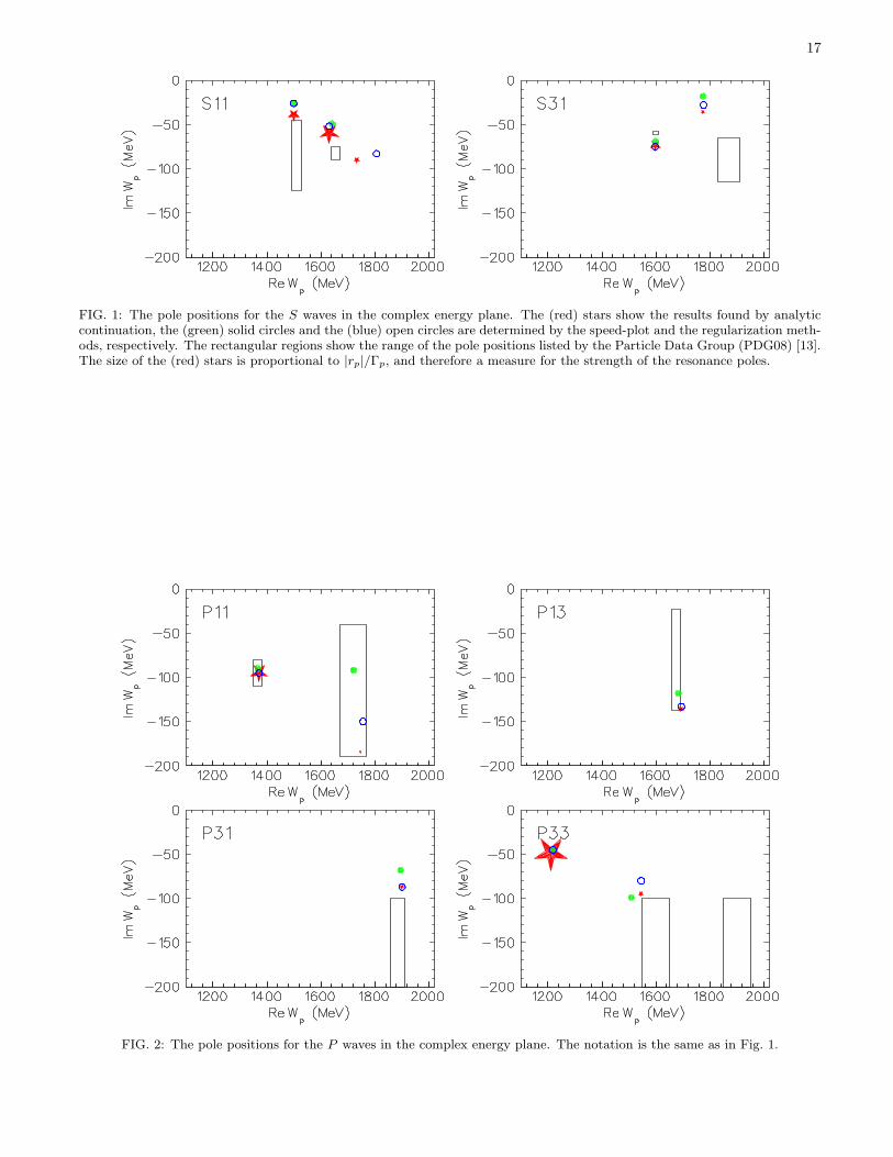
A. S waves

As reported in Ref. [54], we need four S11 resonances to fit the πN scattering amplitude in this channel, instead of

only three resonances listed by PDG [13]. The additional resonance S11(1880) was found to play an important role

in pion photoproduction as well [54], but was not seen in both the πN → ηN reaction and recent measurements of

η photoproduction from the proton [64, 65]. However, in the analysis of Saghai et al. [66] on eta photoproduction a

new S11 state of mass M = 1707 MeV and width Γ = 222 MeV was needed in order to get good agreement with the

data.

In our analysis we find three poles below 2 GeV (see Fig. 1, left panel). The exact pole positions are shown by

asterisks with a size indicating the relative strength, proportional to |rp|/Γp. Furthermore, the ranges of the PDG

pole values are displayed by open boxes. The first resonance S11(1535)∗∗∗∗ is found by both SP and RM. The second

state, the S11(1650)∗∗∗∗ is somewhat better described by RM. The third S11 state is very weakly excited by πN

scattering and not seen by SP, whereas RM finds a nearby state. In our analysis and many others as well, the S11

is the most problematic partial wave due to the inelastic η threshold and two overlapping resonances with large

residues. Whereas the real part of the pole positions, the pole mass Mp of the 4-star resonances are exactly found,

the widths Γp are considerably underpredicted by RM. The situation is even worse for the moduli of the residues,

which show a very bad convergence with order N . Of course, the problem has been known before. A large variation

among different partial wave analyses can be found in the literature, which reflects itself in the large error bars of the

PDG pole parameters for the S11(1535) resonance. The problem can be quantitatively expressed by the closeness of

nearby singularities, with distances obtained from the central values of the PDG listing. Seen from the pole position

of the S11(1535), the nearest singularities are the η threshold and the S11(1650) pole at distances of 89 MeV and

145 MeV, respectively. On the other hand, the S11(1535) pole lies 85 MeV away from the real axis. As a consequence,

the Taylor expansion of the regular function T reg in Eq. (11) comes close to its convergence circle if we extrapolate

to the real axis. Therefore, the analytical continuation into the complex plane is strongly recommended instead of

12

the extrapolation. Nevertheless, if the extrapolation fails, also the exact pole parameters of a model have to be taken

with a grain of salt.

For the isospin 3/2 states we obtain three poles in agreement with PDG. The first one, S31(1620)∗∗∗∗, is nicely

described by SP and perfectly by RM. The position of the second pole, S31(1900)∗∗, is similarly well seen by both SP

and RM. However, the modulus of the residue is strongly underestimated.

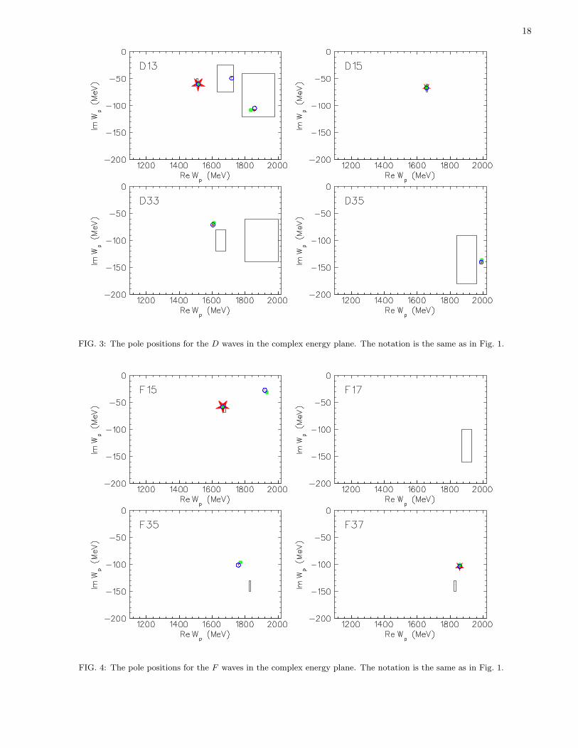
B. P waves

For the P -wave resonances we show our results in Fig. 2. In the P11 partial wave the DMT predicts two poles well

inside the PDG boxes. However, the second pole lies near the lower edge of the box. The resonance parameters of

the Roper or P11(1440)∗∗∗∗ are nicely reproduced by both SP and RM. The P11(1710)∗∗∗∗ has a very weak signal in

the πN channel. Although the RM yields a considerable improvement over the SP, it misses the exact pole position

and the phase of the residue.

In the P13 partial wave we only find one pole below 2 GeV, while PDG lists two states, the P13(1720)∗∗∗∗ with a

large error bar for the imaginary part and the P13(1900)∗∗, however, with no pole position given. Our results for the

P13(1720) lie close to the PDG values, with the imaginary part near to the lower limit of the PDG error bar. The

RM reproduces the pole parameters of the P13(1720)∗∗∗∗ quite well.

In the isospin-3/2 partial wave, we find the pole of the P31(1910)∗∗∗∗ slightly outside the PDG box. All the pole

parameters are well described by RM.

The Delta resonance, P33(1232)∗∗∗∗, has, of course, the largest strength of all the poles found by our analysis. The

analytic pole values are well described by both the SP and RM techniques, they also agree with the PDG listing. Due

to numerical instabilities in the region of the first resonance, the RM fails for higher-order derivatives, and therefore

this method can not much improve on the SP result. As a result the RM values differ slightly from the parameters

obtained by analytical continuation. Another weakly excited P33 state is found at higher energy, which can be related

to the state P33(1600)∗∗∗ of PDG. The pole parameters of this second state converge well within RM. The third PDG

resonance shown in Fig. 2, P33(1920)∗∗∗, appears at an energy above 2 GeV in the DMT model.

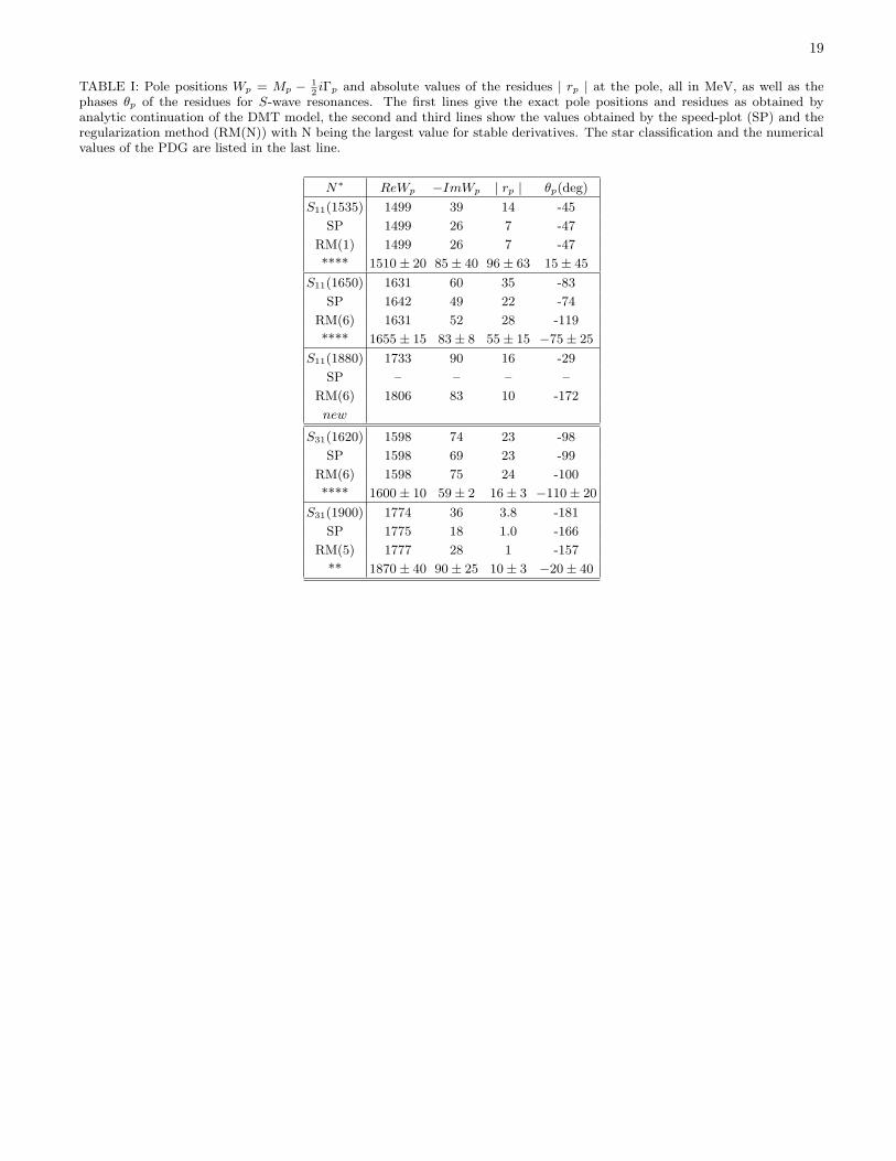
C. D waves

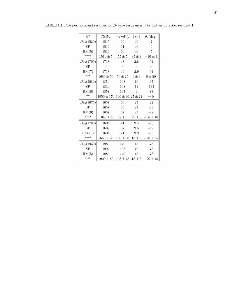
In Fig. 3 we display the poles of D-wave resonances. PDG lists three J = 3/2 states with isospin 1/2, D13(1520)∗∗∗∗,

D13(1700)∗∗∗, and D13(2080)∗∗, and the DMT agrees very well within the reported ranges. Except for the residue

of the D13(2080), we find a perfect convergence of the RM for the pole positions and residues. The D13(1700) is a

particular case, for which the SP can not find the pole, whereas the higher-order derivatives of the RM yield very

precise results.

For the D15 partial wave we find a rather simple contour with only one resonance, D15(1675)∗∗∗∗, below 2 GeV.

There is perfect agreement among the exact DMT values, the SP and RM extrapolations as well as the PDG listings.

13

For the isospin-3/2 D-wave resonances, PDG reports only one 4-star resonance, the D33(1700)∗∗∗∗. Our analytic

results are well reproduced by SP and perfectly by RM. A similar agreement is also found for the D35(1930)∗∗∗. Both

resonances are located very close to the PDG boxes.

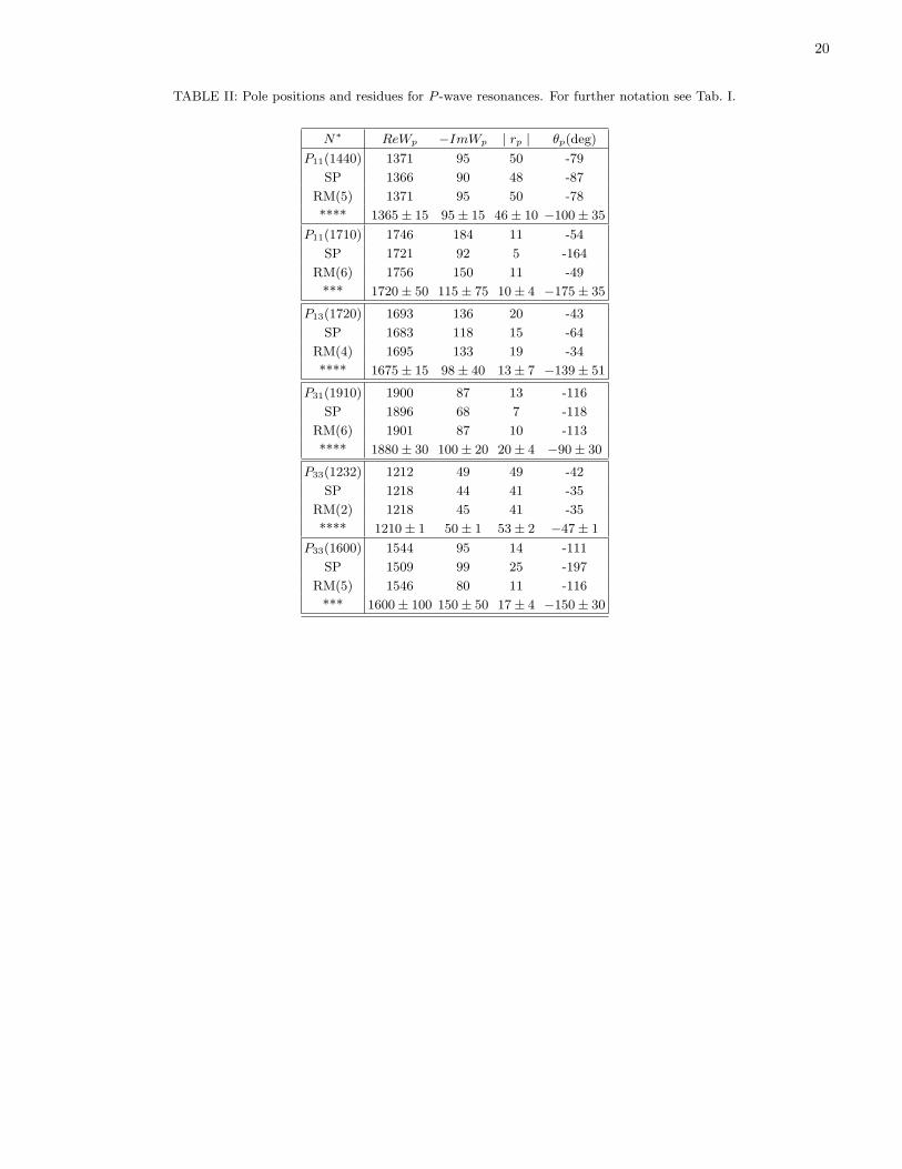
D. F waves

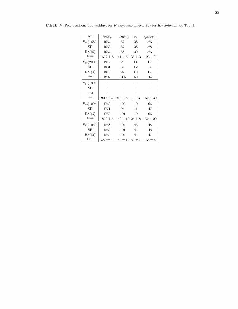
Figure 4 displays the F -wave resonances. The F15(1680)∗∗∗∗ is the most important resonance in the 3rd resonance

region. The exact DMT pole parameters are perfectly described by SP and RM. We also find a second F15 state

with a small residue |rp| ∼ 1 GeV. Because of its location close to the real axis, this state is also well described by

SP and RM. In its vicinity, PDG reports the F15(2000)∗∗ resonance, however, with no pole parameters given. In the

F17 partial wave we can not find a resonance by our analysis, whereas PDG lists a F17(1990)∗∗. Our result is based

on the fact that the inclusion of a bare resonance in this partial wave does not significantly improve the χ2 fit to the

data. A similar conclusion was obtained in Refs. [11, 12].

For the isospin-3/2 resonances, we find two poles corresponding to the states F35(1905)∗∗∗∗ and F37(1950)∗∗∗∗

reported by PDG. The pole parameters of the DMT are nicely described by SP and RM for both these resonances.

However, our pole positions lie significantly above the PDG bounds for the imaginary values. This disagreement is

not too surprising, because the uncertainty of a pole position rises with the distance from the real axis. In conclusion,

RM converges well for the F wave amplitudes, and all pole positions and residues are obtained in full agreement with

the results of the analytical continuation.

V. SUMMARY AND CONCLUSION

Within our previously developed Dubna-Mainz-Taipei (DMT) dynamical model, we have investigated the pole

structure of the pion-nucleon T matrix for all S, P , D, and F partial waves in the energy range up to the c.m. energy

W = 2.0 GeV. For this purpose, the solutions of our coupled integral equations were (i) analytically continued to

unphysical energies in the range 0 > ImW ≥ −200 MeV, (ii) mapped by contour plots, and (iii) searched for poles

in the regions of interest. The resulting pole positions and residues were compared to approximative solutions as

obtained by the speed plot (SP), based on the first derivative of the amplitude at physical energies, and the recently

developed regularization method (RM), based on higher derivatives.

The number and positions of the DMT poles, as found by a newly developed analytic continuation method, are in

good agreement with the current results of the Particle Data Group (PDG) [13], all except for the S11 partial waves.

In particular for the S11(1535)∗∗∗∗ and S11(1650)∗∗∗∗ resonances, the DMT model yields much smaller widths and

residues than listed by PDG. Furthermore, the model predicts an additional S11(1880) resonance.

Let us now turn to the main issue of our work: How well can we determine a given pole structure by our knowledge

of the experimental data, that is, on the basis of the scattering amplitudes for physical energies. For that purpose we

use our DMT amplitudes at physical energies as interpolating functions for the single-energy partial wave amplitudes

that were obtained from the experimental data. These numerically differentiable functions serve as input for the

SP and RM techniques. The approximative pole positions and residues are then compared to the exact predictions

of DMT, as determined by analytic continuation of the integral equations. The results for the partial waves are

14

summarized as follows:

S waves: The pole structure of the resonance S11(1535)∗∗∗∗ is the most problematic feature of our findings.

Although the RM reproduces the real parts of the pole positions (Mp), it underpredicts the widths (Γp) and the

moduli of the residues (|rp|). However, problems with this resonance appear also in many other analyses. This is

clearly visible in the large uncertainties of the respective PDG values. The reason for the failure is two-fold: (i)

The two four-star resonances overlap substantially and (ii) the eta threshold lies close to the first resonance. The

RM is based on the convergence of the Laurent series about the pole position in order to extrapolate from the pole

to the data on the real axis and vice versa. However, the extrapolation from the S11(1535) pole to the real axis

involves energies close to the convergence circle, which is determined by the distance between pole and eta threshold.

Even worse, the input for the RM are data taken at Mp ≈ 1500 MeV, only 25 MeV above eta threshold. This

threshold enters in two ways: (i) The inelasticity lowers both the pion-nucleon branching ratio and the pole residue

by about 50% and (ii) the eta yields about half of the total width. Both effects are strongly energy dependent near

the eta threshold and contrary to the assumption of RM, the regular part of the Laurent expansion changes rapidly

as a function of energy because of the nearby eta cusp. As a consequence, there is no convergence of the RM if

applied to the S11(1535). Already the second derivative of the amplitude yields numerical noise with regard to the

pole properties. By comparison with the first resonance, the S11(1650)∗∗∗∗ state is much better described by RM,

although the values for the width and the residue are not fully satisfactory, possibly because of the mixing with the

problematic S11(1535)∗∗∗∗ resonance. In the isospin 3/2 channel, the S31(1620)∗∗∗∗ is perfectly described, whereas

the RM result for the S31(1900)∗∗ differs in some respects from the exact solution. Of course, this weak two-star

resonance is more difficult to find, and also the PDG lists large error bars for the pole parameters.

P waves: For most of the P wave resonances, RM converges well and yields rather precise pole parameters in

the range of 4-6 differentiations. Only the P11(1710)∗∗∗ results are somewhat problematic, which is also reflected by

large error bars given by PDG. A minor irregularity is observed for the P33(1232)∗∗∗∗. Because of some numerical

instability, the RM does not converge, and therefore the SP results can not be improved.

D and F waves: Already the SP yields quite reasonable values in most cases, and after 4-7 differentiations RM

converges to the exact values of the pole parameters. In general, these resonances are pretty isolated and threshold

effects are suppressed for the higher partial waves. An interesting case is the D13(1700)∗∗∗, which is not seen by SP

but correctly described by RM. Furthermore, the resonance F17(1990)∗∗ listed by PDG with a width of 260 MeV is

not found by the DMT fit to the data.

We conclude that the regularization method is a reliable method to extract the pole structure from single-channel

data. In the absence of full experimental knowledge about all of the channels, this method can be sequentially applied

in order to determine the pole structure relevant for the experimentally known channels of a multichannel system.

However, the method loses its predictive power in regions of nearby thresholds and strongly overlapping resonances.

In such cases, only an analytic continuation of the model can fully determine the structure of the singularities. Of

course, such a model must describe the experimental multichannel amplitudes by a “global fit” over a large energy

range. On the other hand, the regularization method is also useful when it falls short because such failure signals a

complicated singularity structure of the scattering amplitude.

15

Acknowledgment

S.S.K. wishes to acknowledge the financial support from the National Science Council and National Center for

Theoretical Sciences of ROC for his visits to the Physics Department of National Taiwan University. The work of

S.N.Y. is supported in part by the NSC/ROC under grant No. NSC98-2112-M002-006. We are also grateful for the

support by the Deutsche Forschungsgemeinschaft through SFB 443, the joint project NSC/DFG 446 TAI113/10/0-3,

and the joint Russian-German Heisenberg-Landau program.

[1] H.L. Anderson, E. Fermi, E.A. Long, R. Martin, and D.E. Nagle, Phys. Rev. 85, 934 (1952).[2] E. Fermi, H.L. Anderson, A. Lundby, D.E. Nagle, and G.B. Yodh, Phys. Rev. 85, 935 (1952).[3] H.L. Anderson, E. Fermi, E.A. Long, and D.E. Nagle, Phys. Rev. 85, 936 (1952).[4] A. Donnachie, Springer Tracts Mod. Phys. 61, 25 (1972).[5] A. Donnachie, Reports on Progress in Physics 36, 695 (1973).[6] G. Hohler, F. Kaiser, R. Koch, and E. Pietarinen, Handbook of Pion-Nucleon Scattering , Physics Data 12-1, FIZ Karlsruhe

(1979).[7] R. Koch and E. Pietarinen, Nucl. Phys. A336, 331 (1980).[8] R.E. Cutkosky, R.E. Hendrick, J.W. Alcock, Y.A. Chao, R.G. Lipes, J.C. Sandusky and R.L. Kelly, Phys. Rev. D 20, 2804

(1979).[9] R.E. Cutkosky, C.P. Forsyth, R.E. Hendrick and R.L. Kelly, Phys. Rev. D 20, 2839 (1979).

[10] R.A. Arndt, J.M. Ford, and L.D. Roper, Phys. Rev. D 32, 1085 (1985).[11] R.A. Arndt, W.J. Briscoe, I.I. Strakovsky, R.L. Workman, and M.M. Pavan, Phys. Rev. C 69, 035213 (2004).[12] R.A. Arndt, W.J. Briscoe, I.I. Strakovsky, and R.L. Workman, Phys. Rev. C 74, 045205 (2006).[13] C. Amsler, et al. (Particle Data Group), Phys. Lett. B 667, 1 (2008) and K. Nakamura, et al. (Particle Data Group), J.

Phys. G 37, 075021 (2010).[14] W.N. Cottingham, D.A. Greenwood, “An Introduction to Nuclear Physics”, Cambridge University Press, Cambridge 1986

and 2001.[15] R.H. Dalitz and R.G. Moorhouse, Proc. R. Soc. London A 318, 279 (1970).[16] D. Djukanovic, J. Gegelia and S. Scherer, Phys. Rev. D 76, 037501 (2007).[17] J. Gegelia and S. Scherer, Eur. Phys. Jour. A 44, 425 (2010).[18] G. Hohler, In NSTAR2001, Proceedings of the Workshop on The Physics of Excited Nucleons, ed. D. Drechsel and L.

Tiator, World Scientific 2001, 185.[19] G.F. Chew, Berkeley UCRL-16983 (1966).[20] G. Hohler, D.E. Groom et al., Particle Data Group, Eur. Phys. Jour. C 15, 1 (2000).[21] G. Hohler and A. Schulte, PiN Newslett. 7, 94 (1992).[22] S. Ceci, J. Stahov, A. Svarc, S. Watson, and B. Zauner, Phys. Rev. D 77, 116007 (2008).[23] C. Alexandrou, Proc. of NSTAR2009, Beijing, China, 2009, arXiv:0906.4137 [hep-lat].[24] A. Walker-Loud et al., Phys. Rev. D 79, 054502 (2009).[25] J. Bulava et al., arXiv:1004.5072 [hep-lat].[26] V. Pascalutsa, M. Vanderhaeghen, and S.N. Yang, Phys. Rept. 437, 125 (2007).[27] M. Luscher, Math. Phys. 105, 153 (1986), Nucl. Phys. B 354, 531 (1991) and Nucl. Phys. B 364, 237 (1991).[28] S. Aoki et al., Phys. Rev. D 76, 094506 (2007).[29] V. Bernard, M. Lage, U.G. Meissner and A. Rusetsky, JHEP 0808, 024 (2008).[30] G.Y. Chen, S.S. Kamalov, S.N. Yang, D. Drechsel, and L. Tiator, Phys. Rev. C 76, 035206 (2007).[31] A. Matsuyama, T. Sato, and T.-S.H. Lee, Phys. Rept. 439, 193 (2007).[32] B. Julia-Diaz, T.-S.H. Lee, A. Matsuyama, and T. Sato, Phys. Rev. C 76, 065201 (2007).[33] V. Shklyar, H. Lenske, U. Mosel, and G. Penner, Phys. Rev. C 71, 055206 (2005).[34] M. Doring, C. Hanhart, F. Huang, S. Krewald, and U.-G. Meißner, Nucl. Phys. A829, 170 (2009).[35] T. Inoue, E. Oset and M.J. Vicente Vacas, Phys. Rev. C 65, 035204 (2002).[36] E.E. Kolomeitsev, M.F.M. Lutz, Phys. Lett. B 585, 243 (2004).[37] S.S. Kamalov, G.Y. Chen, S.N. Yang, D. Drechsel, and L. Tiator, Phys. Lett. B 522, 27 (2001).[38] M. Weis et al. [A1 Collaboration], Eur. Phys. J. A 38, 27 (2008).[39] D. Hornidge, Proposal MAMI-A2/6-03 and priv. comm. (2010).[40] L. Eisenbud, Ph.D. dissertation, Princeton University 1948, (unpublished).[41] F.T. Smith, Phys. Rev. 118, 349 (1960).[42] E.P. Wigner, Phys. Rev. 98, 145 (1955).[43] H.M. Nussenzweig, Phys. Rev. D 6, 1534 (1972).[44] N. Suzuki, T. Sato, and T.-S.H. Lee, Phys. Rev. C 79, 025205 (2009).

16

[45] H. Haberzettl and R. Workman, Phys. Rev. C 76, 058201 (2007).[46] J. von Neumann, E.P. Wigner, Physik. Z. 30, 467 (1929).[47] S. Ceci et al., Phys. Lett. B 659, 228 (2008).[48] R.L. Workman, R.A. Arndt, M.W. Paris, Phys. Rev. C 79, 038201 (2009).[49] A. Rittenberg et al., (Review of particle properties - particle data group), Rev. Mod. Phys. 43, S97 (1971).[50] G. Hohler in Landolt-Bornstein: Elastic and Charge Exchange Scattering of Elementary Particles (Springer-Verlag 1983).[51] C.C. Lee, S.N. Yang, and T.-S.H. Lee, J. Phys. G17, L131(1991).[52] C.T. Hung, S.N. Yang, and T.-S.H. Lee, J. Phys. G20, 1531 (1994).[53] C.T. Hung, S.N. Yang, and T.-S.H. Lee, Phys. Rev. C 64, 034309 (2001).[54] G.Y. Chen, S.S. Kamalov, S.N. Yang, D. Drechsel, and L. Tiator, Nucl. Phys. A 723, 447 (2003).[55] SAID partial wave analysis, solution FA02, Ref. [11].[56] S.S. Kamalov and S.N. Yang, Phys. Rev. Lett. 83, 4494 (1999).[57] S.S. Kamalov, S.N. Yang, D. Drechsel, O. Hanstein, and L. Tiator, Phys. Rev. C 64, 032201(R) (2001).[58] E.D. Cooper and B.K. Jennings, Nucl. Phys. A 483, 601 (1988).[59] S. Morioka and I.R. Afnan, Phys. Rev. C 26, 1148 (1982).[60] B.C. Pearce and I.R. Afnan, Phys. Rev. C 34, 991 (1986).[61] L. Tiator, C. Bennhold, and S.S. Kamalov, Nucl. Phys. A 580, 455 (1994).[62] A.I. L’vov, V.A. Petrun’kin, and M. Schumacher, Phys. Rev. C 55, 359 (1997).[63] D. Drechsel, O. Hanstein, S.S. Kamalov, and L. Tiator, Nucl. Phys. A 645, 145 (1999).[64] U. Thoma, Int. J. Mod. Phys. A 20, 1568 (2005).[65] D. Elsner et al. (CBELSA), Eur. Phys. J. A 33, 147 (2007).[66] B. Saghai, J. Durand, B. Julia-Diaz, HE Jun, T.-S.H. Lee, and T. Sato, Chinese Physics (HEP & NP) 33, 1175 (2009).

17

FIG. 1: The pole positions for the S waves in the complex energy plane. The (red) stars show the results found by analyticcontinuation, the (green) solid circles and the (blue) open circles are determined by the speed-plot and the regularization meth-ods, respectively. The rectangular regions show the range of the pole positions listed by the Particle Data Group (PDG08) [13].The size of the (red) stars is proportional to |rp|/Γp, and therefore a measure for the strength of the resonance poles.

FIG. 2: The pole positions for the P waves in the complex energy plane. The notation is the same as in Fig. 1.

18

FIG. 3: The pole positions for the D waves in the complex energy plane. The notation is the same as in Fig. 1.

FIG. 4: The pole positions for the F waves in the complex energy plane. The notation is the same as in Fig. 1.

19

TABLE I: Pole positions Wp = Mp − 12iΓp and absolute values of the residues | rp | at the pole, all in MeV, as well as the

phases θp of the residues for S-wave resonances. The first lines give the exact pole positions and residues as obtained byanalytic continuation of the DMT model, the second and third lines show the values obtained by the speed-plot (SP) and theregularization method (RM(N)) with N being the largest value for stable derivatives. The star classification and the numericalvalues of the PDG are listed in the last line.

N∗ ReWp −ImWp | rp | θp(deg)

S11(1535) 1499 39 14 -45

SP 1499 26 7 -47

RM(1) 1499 26 7 -47

**** 1510± 20 85± 40 96± 63 15± 45

S11(1650) 1631 60 35 -83

SP 1642 49 22 -74

RM(6) 1631 52 28 -119

**** 1655± 15 83± 8 55± 15 −75± 25

S11(1880) 1733 90 16 -29

SP – – – –

RM(6) 1806 83 10 -172

new

S31(1620) 1598 74 23 -98

SP 1598 69 23 -99

RM(6) 1598 75 24 -100

**** 1600± 10 59± 2 16± 3 −110± 20

S31(1900) 1774 36 3.8 -181

SP 1775 18 1.0 -166

RM(5) 1777 28 1 -157

** 1870± 40 90± 25 10± 3 −20± 40

20

TABLE II: Pole positions and residues for P -wave resonances. For further notation see Tab. I.

N∗ ReWp −ImWp | rp | θp(deg)

P11(1440) 1371 95 50 -79

SP 1366 90 48 -87

RM(5) 1371 95 50 -78

**** 1365± 15 95± 15 46± 10 −100± 35

P11(1710) 1746 184 11 -54

SP 1721 92 5 -164

RM(6) 1756 150 11 -49

*** 1720± 50 115± 75 10± 4 −175± 35

P13(1720) 1693 136 20 -43

SP 1683 118 15 -64

RM(4) 1695 133 19 -34

**** 1675± 15 98± 40 13± 7 −139± 51

P31(1910) 1900 87 13 -116

SP 1896 68 7 -118

RM(6) 1901 87 10 -113

**** 1880± 30 100± 20 20± 4 −90± 30

P33(1232) 1212 49 49 -42

SP 1218 44 41 -35

RM(2) 1218 45 41 -35

**** 1210± 1 50± 1 53± 2 −47± 1

P33(1600) 1544 95 14 -111

SP 1509 99 25 -197

RM(5) 1546 80 11 -116

*** 1600± 100 150± 50 17± 4 −150± 30

21

TABLE III: Pole positions and residues for D-wave resonances. For further notation see Tab. I.

N∗ ReWp −ImWp | rp | θp(deg)

D13(1520) 1515 60 40 -7

SP 1516 61 40 -6

RM(5) 1516 60 40 -5

**** 1510± 5 55± 5 35± 3 −10± 4

D13(1700) 1718 48 2.8 -91

SP – – – –

RM(7) 1718 49 2.9 -91

*** 1680± 50 50± 25 6± 3 0± 50

D13(2080) 1854 108 16 -97

SP 1834 108 14 -134

RM(6) 1858 105 9 -83

** 1950± 170 100± 40 27± 22 ∼ 0

D15(1675) 1657 66 24 -22

SP 1657 66 24 -23

RM(6) 1657 67 25 -22

**** 1660± 5 68± 6 29± 6 −30± 10

D33(1700) 1604 71 9.4 -63

SP 1609 67 9.5 -52

RM (6) 1604 71 9.9 -63

**** 1650± 30 100± 20 13± 3 −20± 25

D35(1930) 1989 140 18 -78

SP 1992 136 19 -75

RM(5) 1989 140 18 -78

*** 1900± 50 133± 48 18± 6 −20± 40

22

TABLE IV: Pole positions and residues for F -wave resonances. For further notation see Tab. I.

N∗ ReWp −ImWp | rp | θp(deg)

F15(1680) 1664 57 38 -26

SP 1663 57 38 -28

RM(6) 1664 58 39 -26

**** 1672± 8 61± 6 38± 3 −23± 7

F15(2000) 1919 26 1.0 15

SP 1931 31 1.3 89

RM(4) 1919 27 1.1 15

** 1807 54.5 60 −67

F17(1990) – – – –

SP – – – –

RM – – – –

** 1900± 30 260± 60 9± 3 −60± 30

F35(1905) 1760 100 10 -66

SP 1771 96 11 -47

RM(5) 1759 101 10 -66

**** 1830± 5 140± 10 25± 8 −50± 20

F37(1950) 1858 104 43 -48

SP 1860 101 44 -45

RM(5) 1859 104 44 -47

**** 1880± 10 140± 10 50± 7 −33± 8