Self-attenuation

Marie-Christine Lépy

Laboratoire National Henri Becquerel - LNE / CEA-DRT-LIST

CEA Saclay – F-91191 GIF-SUR-YVETTE Cedex - FRANCE

E-mail : marie-christine.lepy@cea.fr

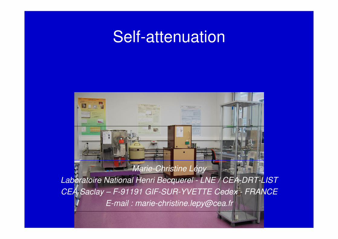
Self-attenuation

• Introduction

• Attenuation coefficients

• Self-attenuation

– Simple analytical formula

– Generalisation

– Practical tools

• Examples

Introduction

• Emission of photons attenuated through the

sample

• If sample different from the calibration (size,

shape, density, chemical composition)

– Reduction of the photon beam

– « False » peak areas

– Correction factor required to get the true activity

• Homogeneity ?

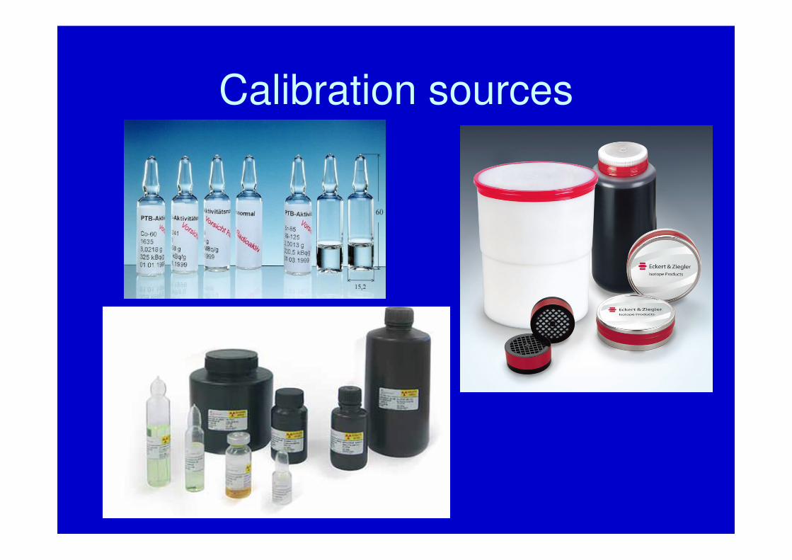
Calibration sources

Attenuation coefficients

• Definition – Beer-Lambert law

• Tables

• Experimental measurement

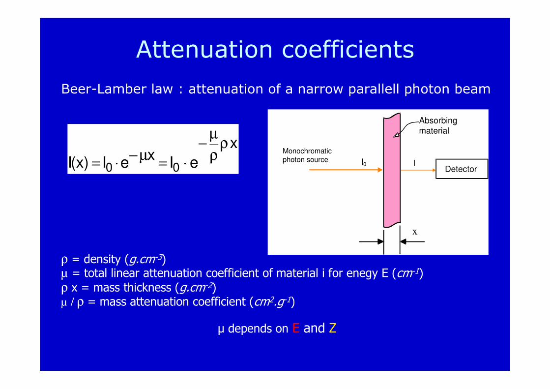
Beer-Lamber law : attenuation of a narrow parallell photon beam

ρ = density (g.cm-3)µ = total linear attenuation coefficient of material i for enegy E (cm-1)

ρ x = mass thickness (g.cm-2)µ / ρ = mass attenuation coefficient (cm2.g-1)

µ depends on E and Z

x

eIx

eI)x(I 00

ρρ

µ−

⋅=µ−

⋅=

Attenuation coefficients

Monochromaticphoton source

Absorbing

material

Detector

x

II0

Attenuation coefficients (2)

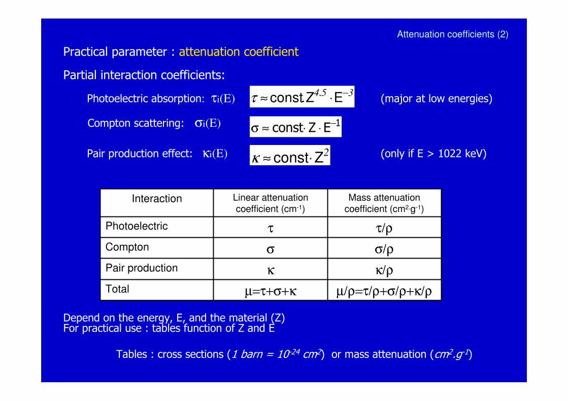
Practical parameter : attenuation coefficient

Partial interaction coefficients:

Photoelectric absorption: τi(E) (major at low energies)

Compton scattering: σi(E)

Pair production effect: κi(E) (only if E > 1022 keV)

Depend on the energy, E, and the material (Z)For practical use : tables function of Z and E

Tables : cross sections (1 barn = 10-24 cm2) or mass attenuation (cm2.g-1)

354 −⋅≈ EZ.const .τ

1EZconst −⋅⋅≈σ

2Zconst⋅≈κ

µ/ρ=τ/ρ+σ/ρ+κ/ρµ=τ+σ+κTotal

κ/ρκPair production

σ/ρσCompton

τ/ρτPhotoelectric

Mass attenuationcoefficient (cm2.g-1)

Linear attenuationcoefficient (cm-1)

Interaction

Attenuation coefficients (3)

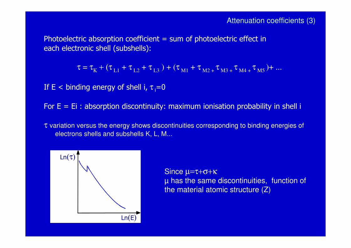
Photoelectric absorption coefficient = sum of photoelectric effect in

each electronic shell (subshells):

τ = τΚ

+ (τL1

+ τL2

+ τL3

) + (τM1

+ τM2 +

τM3 +

τM4 +

τM5

)+ ...

If E < binding energy of shell i, τ i=0

For E = Ei : absorption discontinuity: maximum ionisation probability in shell i

τ variation versus the energy shows discontinuities corresponding to binding energies of

electrons shells and subshells K, L, M...

Ln(τ)

Ln(E)

Since µ=τ+σ+κµ has the same discontinuities, function of the material atomic structure (Z)

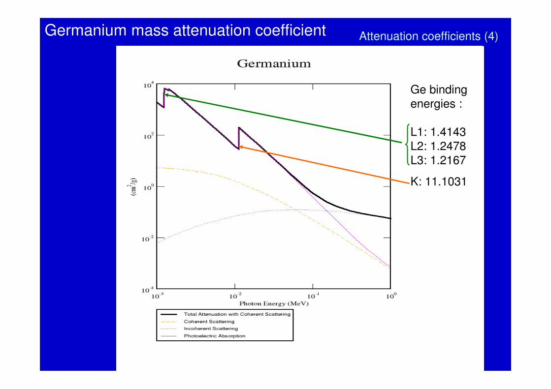
Attenuation coefficients (4)Germanium mass attenuation coefficient

Ge bindingenergies :

L1: 1.4143

L2: 1.2478L3: 1.2167

K: 11.1031

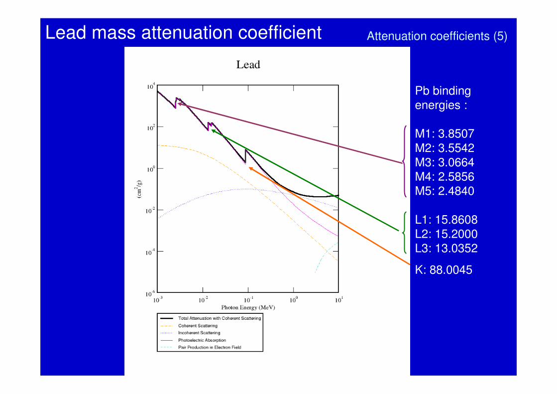
Attenuation coefficients (5)Lead mass attenuation coefficient

Pb bindingenergies :

M1: 3.8507

M2: 3.5542M3: 3.0664M4: 2.5856M5: 2.4840

L1: 15.8608L2: 15.2000L3: 13.0352

K: 88.0045

Mass attenuation coefficients

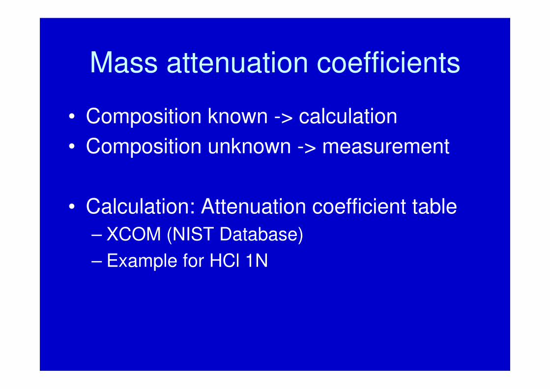
• Composition known -> calculation

• Composition unknown -> measurement

• Calculation: Attenuation coefficient table

– XCOM (NIST Database)

– Example for HCl 1N

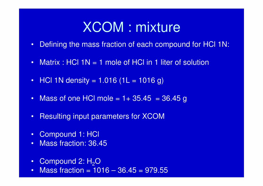
XCOM : mixture• Defining the mass fraction of each compound for HCl 1N:

• Matrix : HCl 1N = 1 mole of HCl in 1 liter of solution

• HCl 1N density = 1.016 (1L = 1016 g)

• Mass of one HCl mole = 1+ 35.45 = 36.45 g

• Resulting input parameters for XCOM

• Compound 1: HCl• Mass fraction: 36.45

• Compound 2: H2O• Mass fraction = 1016 – 36.45 = 979.55

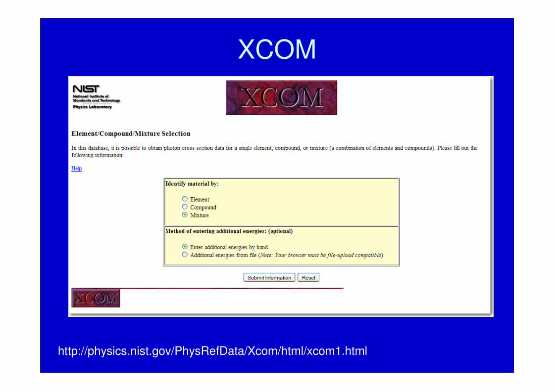
XCOM

http://physics.nist.gov/PhysRefData/Xcom/html/xcom1.html

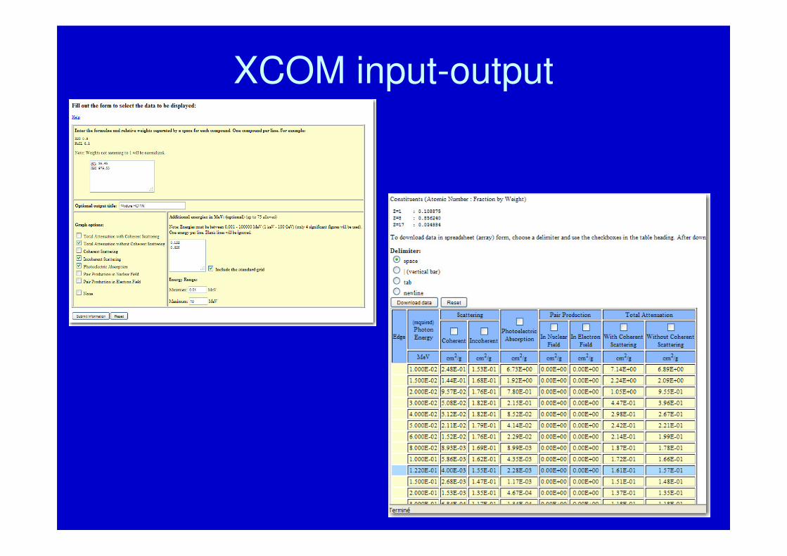
XCOM input-output

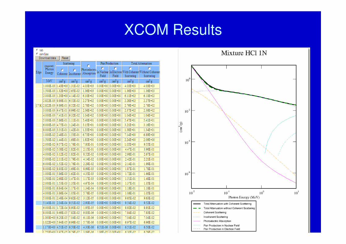
XCOM Results

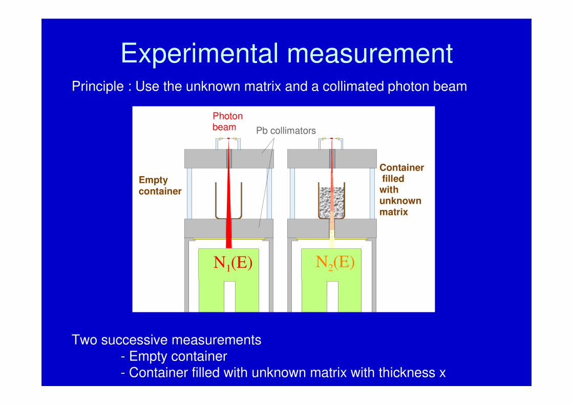
Experimental measurementPrinciple : Use the unknown matrix and a collimated photon beam

Two successive measurements- Empty container- Container filled with unknown matrix with thickness x

Photon beam Pb collimators

Container filled with unknown matrix

N 1 (E) N 2 (E)

Empty container

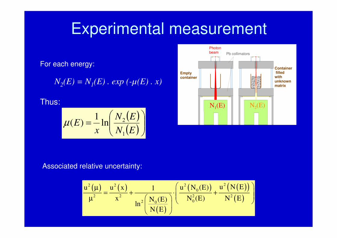
Experimental measurement

For each energy:

N2(E) = N1(E) . exp (-µ(E) . x)

Thus:

( )( )

=

EN

EN

xE

1

2ln1

)(µ

Photon beam Pb collimators

Container filled with unknown matrix

N 1 (E) N 2 (E)

Empty container

( ) ( )

( )

( ) ( )( )( )

222 2

0

2 2 2 2

02 0

u N Eu N (E)u u x 1

x N (E) N EN (E)ln

N E

µ= + ⋅ + µ

Associated relative uncertainty:

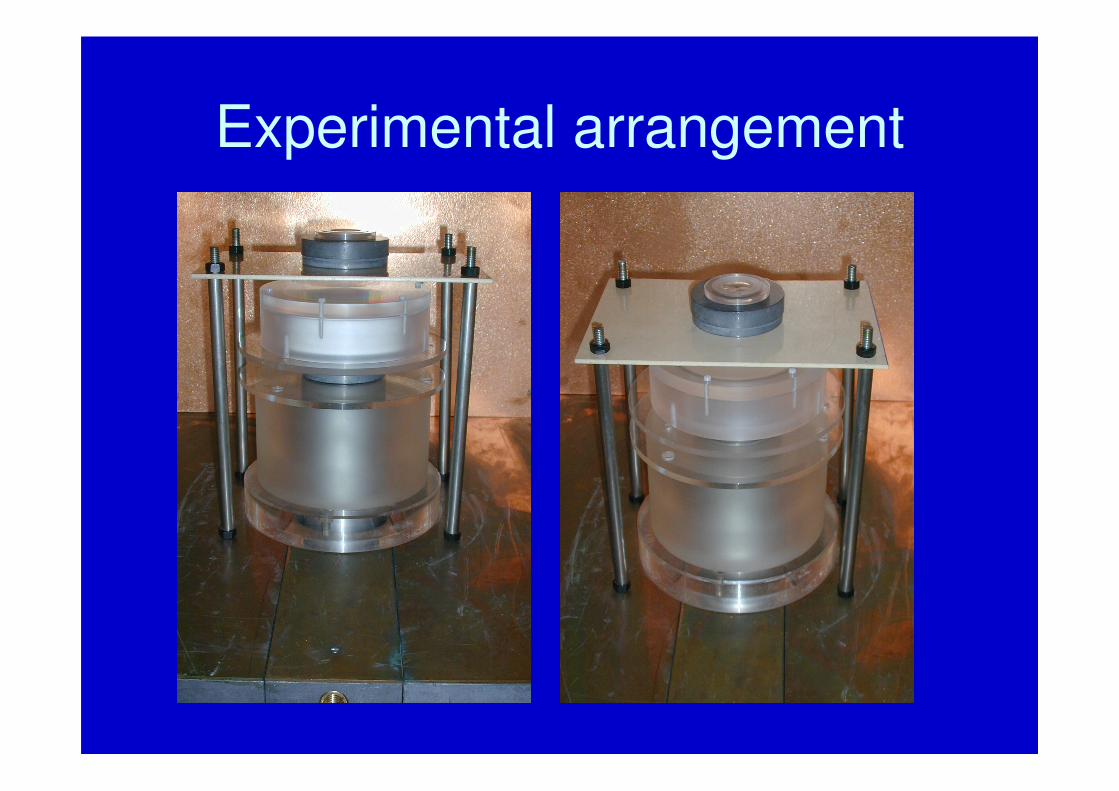
Experimental arrangement

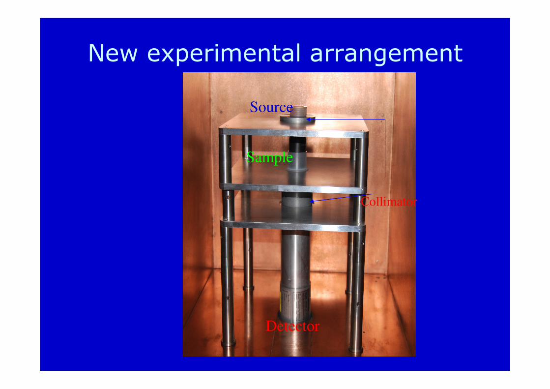
New experimental arrangement

Collimator

Sample

Source

Detector

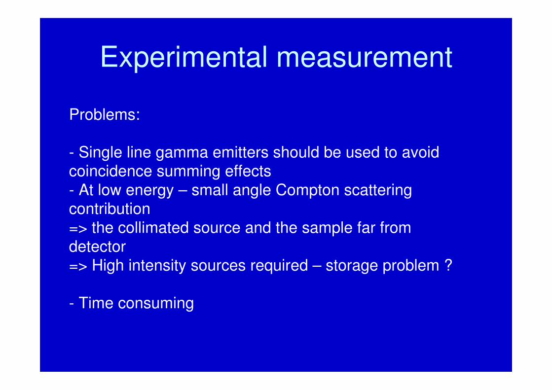
Problems:

- Single line gamma emitters should be used to avoidcoincidence summing effects- At low energy – small angle Compton scatteringcontribution=> the collimated source and the sample far fromdetector=> High intensity sources required – storage problem ?

- Time consuming

Experimental measurement

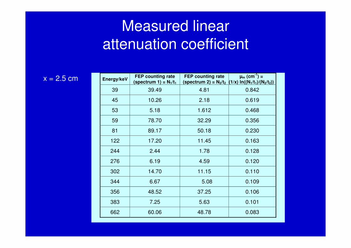
Measured linear

attenuation coefficient

Energy/keV FEP counting rate

(spectrum 1) = N1/t1 FEP counting rate

(spectrum 2) = N2/t2 µm (cm

-1) =

(1/x) ln((N1/t1)/(N2/t2))

39 39.49 4.81 0.842

45 10.26 2.18 0.619

53 5.18 1.612 0.468

59 78.70 32.29 0.356

81 89.17 50.18 0.230

122 17.20 11.45 0.163

244 2.44 1.78 0.128

276 6.19 4.59 0.120

302 14.70 11.15 0.110

344 6.67 5.08 0.109

356 48.52 37.25 0.106

383 7.25 5.63 0.101

662 60.06 48.78 0.083

x = 2.5 cm

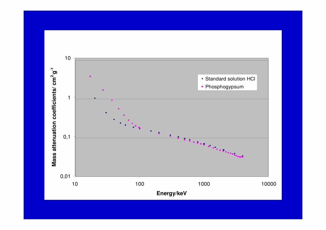
0,01

0,1

1

10

10 100 1000 10000

Energy/keV

Mass a

tten

uati

on

co

eff

icie

nts

/ cm

2. g

-1

Standard solution HClStandard solution HCl

Phosphogypsum

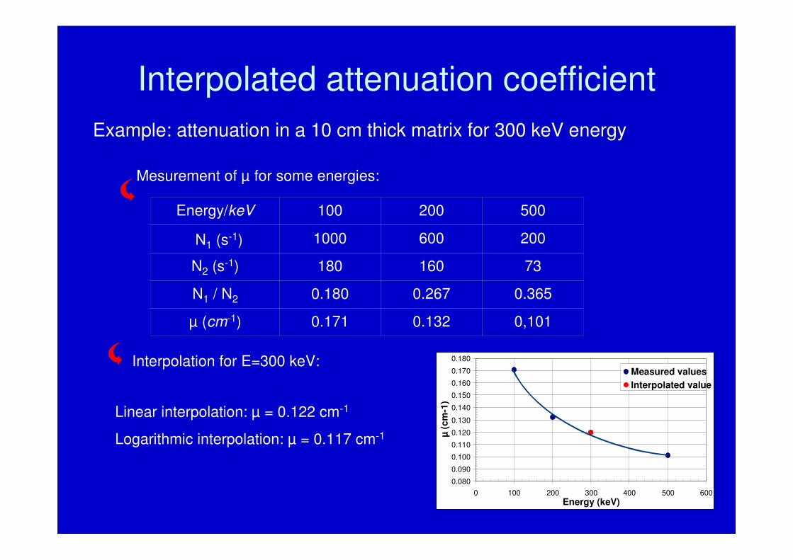
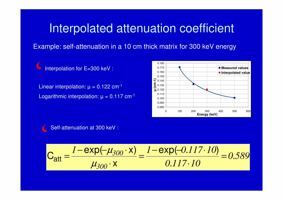
Example: attenuation in a 10 cm thick matrix for 300 keV energy

Energy/keV 100 200 500

1000 600 200

N2 (s-1) 180 160 73

N1 / N2 0.180 0.267 0.365

µ (cm-1) 0.171 0.132 0,101

N1 (s-1)

Mesurement of µ for some energies:

Interpolation for E=300 keV:

Linear interpolation: µ = 0.122 cm-1

Logarithmic interpolation: µ = 0.117 cm-1

Interpolated attenuation coefficient

0.080

0.090

0.100

0.110

0.120

0.130

0.140

0.150

0.160

0.170

0.180

0 100 200 300 400 500 600

Energy (keV)

µ(c

m-1

)

Measured values

Interpolated value

• Software for visualization of the dependence of

interaction coefficients on element and energy

EPICSHOW (NEA databank)

EPICSHOW is part of the EPIC (Electron Photon Interaction Code) system. The program allows interactive viewing and comparison of data in the EPIC data bases.

Plots and listings can be obtained.

The EPIC electron, photon, and charged particle data bases are availablewith this package.

The data bases include data for elements hydrogen (Z=1) to fermium

(Z=100) over the energy range 10 eV to 1 GeV.

Self attenuation

• Simple formula

• Generalisation

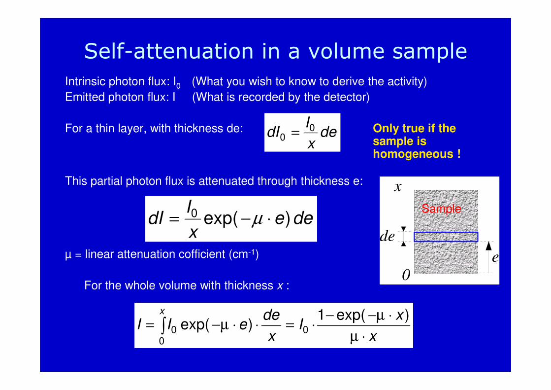
Self-attenuation in a volume sample

Intrinsic photon flux: I0 (What you wish to know to derive the activity)

Emitted photon flux: I (What is recorded by the detector)

For a thin layer, with thickness de: Only true if the sample ishomogeneous !

This partial photon flux is attenuated through thickness e:

µ = linear attenuation cofficient (cm-1)

For the whole volume with thickness x :

x

xI

x

deeII

x

⋅µ

⋅−µ−⋅=⋅⋅−µ= ∫

)exp(1)exp( 0

00

0

x

de

e

deex

IdI )exp(0 ⋅−= µ

dex

IdI 0

0 =

Sample

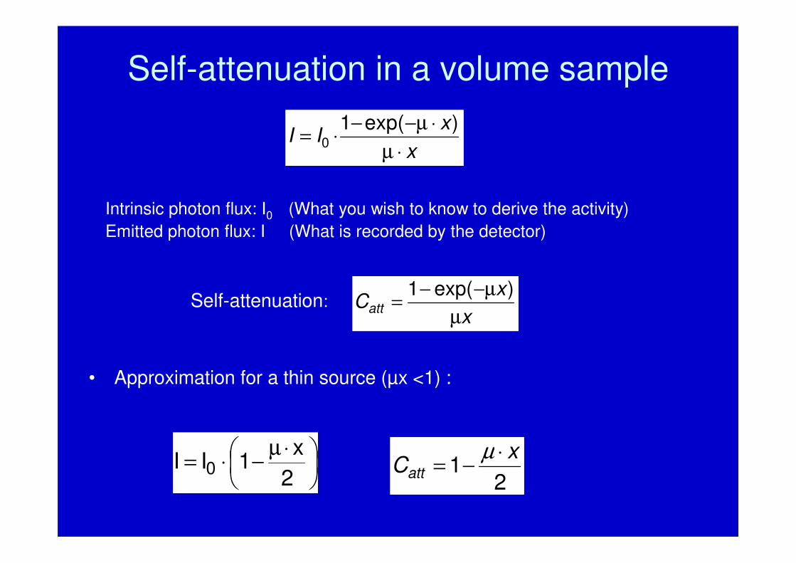
• Approximation for a thin source (µx <1) :

⋅µ−⋅=

2

x1II 0

21

xCatt

⋅−=

µ

x

xCatt

µ

−µ−=

)exp(1Self-attenuation:

Self-attenuation in a volume sample

x

xII

⋅µ

⋅−µ−⋅=

)exp(10

Intrinsic photon flux: I0 (What you wish to know to derive the activity)

Emitted photon flux: I (What is recorded by the detector)

Example: self-attenuation in a 10 cm thick matrix for 300 keV energy

Interpolation for E=300 keV :

Linear interpolation: µ = 0.122 cm-1

Logarithmic interpolation: µ = 0.117 cm-1

Interpolated attenuation coefficient

0.080

0.090

0.100

0.110

0.120

0.130

0.140

0.150

0.160

0.170

0.180

0 100 200 300 400 500 600

Energy (keV)

µ(c

m-1

)

Measured values

Interpolated value

Self-attenuation at 300 keV :

5890101170

10117011

300

300 ..

).exp(

x

)xexp(Catt =

⋅

⋅−−=

⋅

⋅−−=

µ

µ

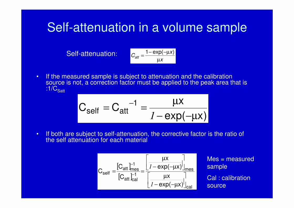
Self-attenuation in a volume sample

• If the measured sample is subject to attenuation and the calibration source is not, a correction factor must be applied to the peak area that is:1/CSatt

• If both are subject to self-attenuation, the corrective factor is the ratio of the self attenuation for each material

x

xCatt

µ

−µ−=

)exp(1

)xexp(

xCC

1attself

−µ−

µ==

−

1

Self-attenuation:

[ ]

[ ]

cal

mes1

calatt

1mesatt

self

)xexp(

x

)xexp(

x

C

CC

−µ−

µ

−µ−

µ

==−

−

1

1

Mes = measuredsample

Cal : calibration source

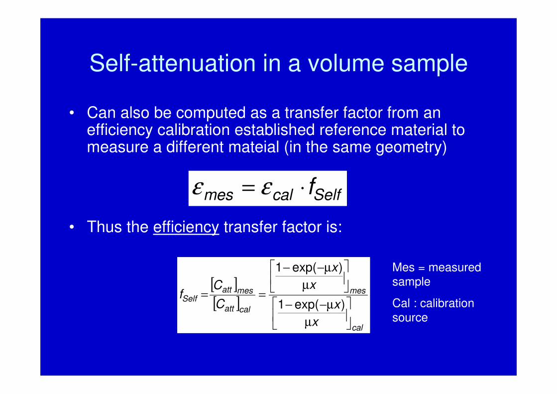
Self-attenuation in a volume sample

• Can also be computed as a transfer factor from an efficiency calibration established reference material to measure a different mateial (in the same geometry)

• Thus the efficiency transfer factor is:

[ ][ ]

cal

mes

calatt

mesattSelf

x

x

x

x

C

Cf

µ

−µ−

µ

−µ−

==)exp(1

)exp(1

Selfcalmes f⋅= εε

Mes = measuredsample

Cal : calibration source

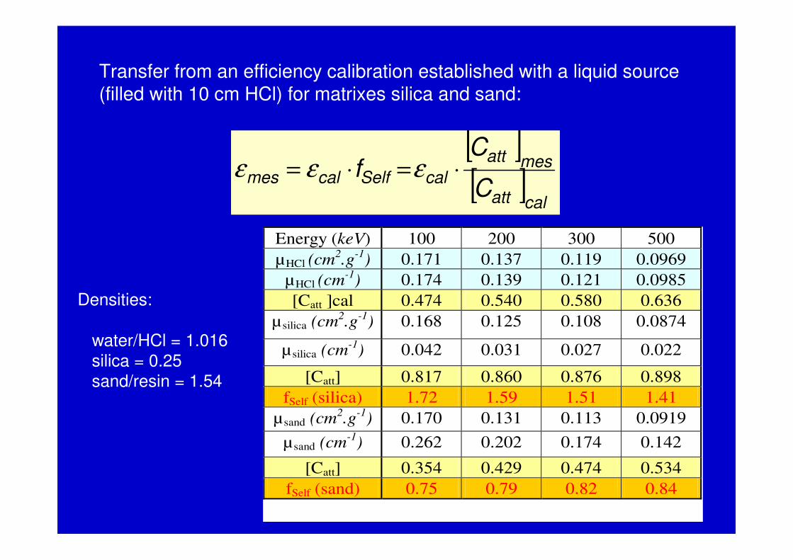
Transfer from an efficiency calibration established with a liquid source (filled with 10 cm HCl) for matrixes silica and sand:

Energy (keV) 100 200 300 500

µHCl (cm2.g

-1) 0.171 0.137 0.119 0.0969

µHCl (cm-1) 0.174 0.139 0.121 0.0985

[Catt ]cal 0.474 0.540 0.580 0.636

µ silica (cm2.g-1) 0.168 0.125 0.108 0.0874

µ silica (cm-1) 0.042 0.031 0.027 0.022

[Catt] 0.817 0.860 0.876 0.898

fSelf (silica) 1.72 1.59 1.51 1.41

µsand (cm2.g-1) 0.170 0.131 0.113 0.0919

µsand (cm-1

) 0.262 0.202 0.174 0.142

[Catt] 0.354 0.429 0.474 0.534

fSelf (sand) 0.75 0.79 0.82 0.84

Densities:

water/HCl = 1.016silica = 0.25sand/resin = 1.54

[ ][ ]

calatt

mesatt

calSelfcalmesC

Cf ⋅=⋅= εεε

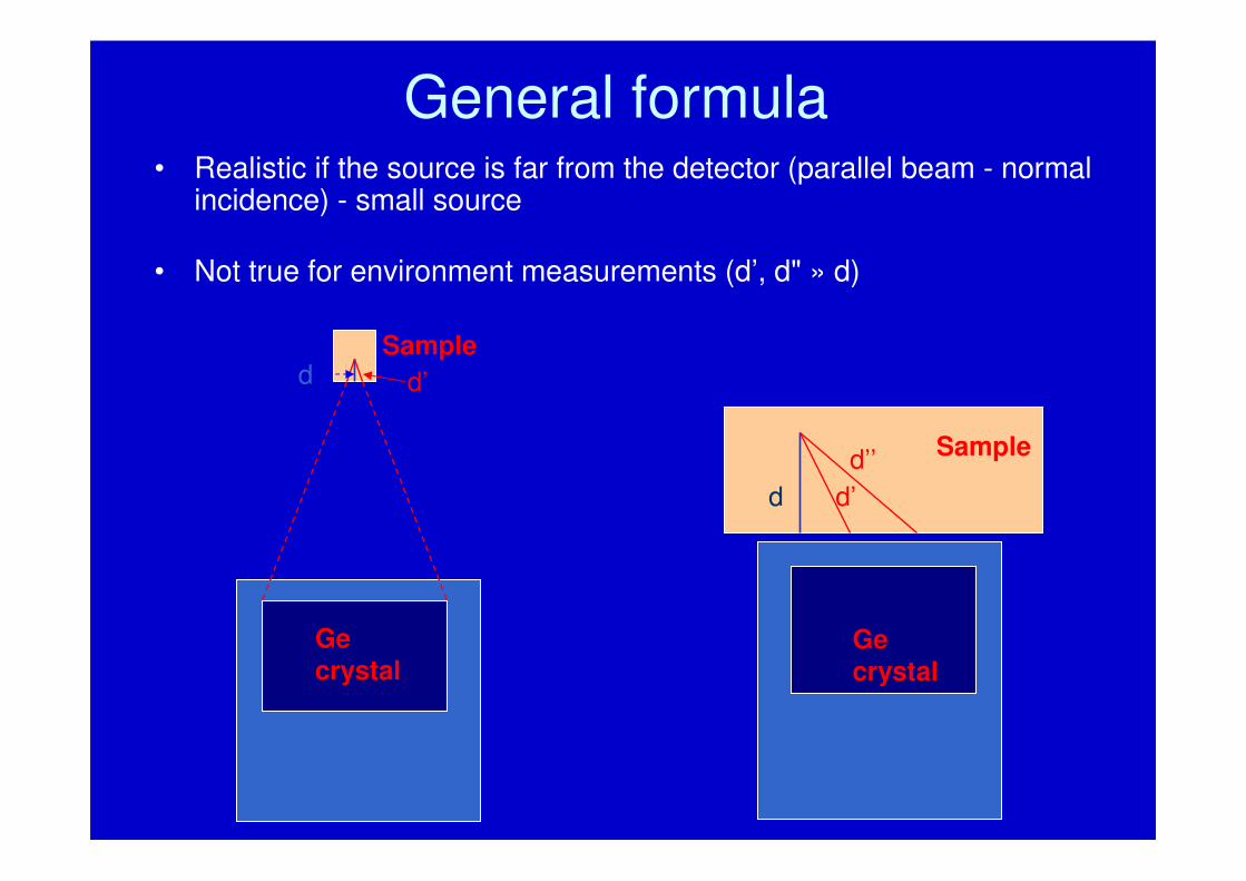
General formula• Realistic if the source is far from the detector (parallel beam - normal

incidence) - small source

• Not true for environment measurements (d’, d" » d)

Sample

Ge crystal

d

d’’

d’

Sample

Ge crystal

d d’

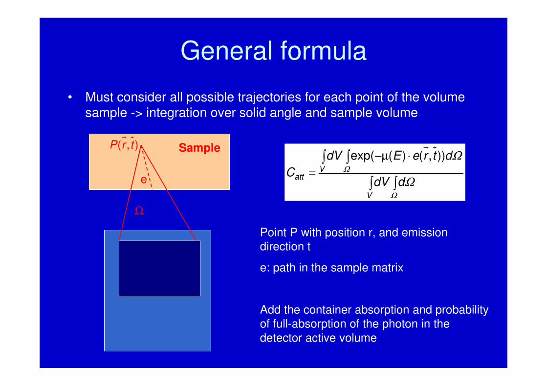
General formula

• Must consider all possible trajectories for each point of the volume sample -> integration over solid angle and sample volume

Point P with position r, and emissiondirection t

e: path in the sample matrix

Add the container absorption and probabilityof full-absorption of the photon in the

detector active volume

∫ ∫

∫ ∫ ⋅−µ

=

V

Vatt

ddV

dtreEdV

C

Ω

Ω

Ω

Ω)),()(exp(Sample

Ω

e

),( trP

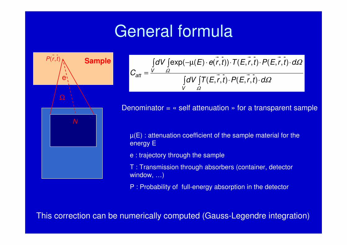
General formula

),( trP Sample

Ω

e

N

∫ ∫

∫ ∫

⋅⋅

⋅⋅⋅⋅−µ

=

V

Vatt

dtrEPtrETdV

dtrEPtrETtreEdV

C

Ω

Ω

Ω

Ω

),,(),,(

),,(),,()),()(exp(

µ(E) : attenuation coefficient of the sample material for the

energy E

e : trajectory through the sample

T : Transmission through absorbers (container, detector

window, …)

P : Probability of full-energy absorption in the detector

Denominator = « self attenuation » for a transparent sample

This correction can be numerically computed (Gauss-Legendre integration)

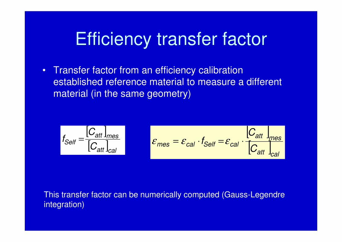
Efficiency transfer factor

• Transfer factor from an efficiency calibration established reference material to measure a differentmaterial (in the same geometry)

[ ][ ]

calatt

mesattSelf

C

Cf =

This transfer factor can be numerically computed (Gauss-Legendre integration)

[ ][ ]

calatt

mesatt

calSelfcalmesC

Cf ⋅=⋅= εεε

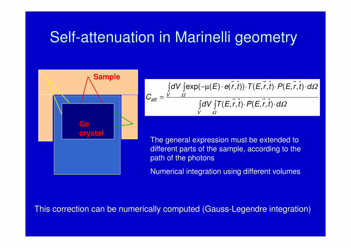
Self-attenuation in Marinelli geometry

∫ ∫

∫ ∫

⋅⋅

⋅⋅⋅⋅−µ

=

V

Vatt

dtrEPtrETdV

dtrEPtrETtreEdV

C

Ω

Ω

Ω

Ω

),,(),,(

),,(),,()),()(exp(

The general expression must be extended to different parts of the sample, according to the path of the photons

Numerical integration using different volumes

Sample

Ge

crystal

This correction can be numerically computed (Gauss-Legendre integration)

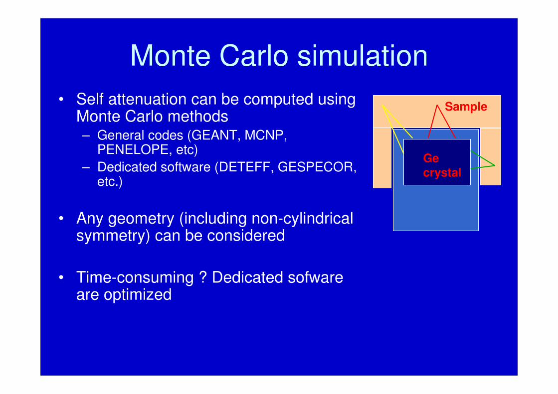
Monte Carlo simulation

• Self attenuation can be computed usingMonte Carlo methods– General codes (GEANT, MCNP,

PENELOPE, etc)

– Dedicated software (DETEFF, GESPECOR, etc.)

• Any geometry (including non-cylindricalsymmetry) can be considered

• Time-consuming ? Dedicated sofwareare optimized

Sample

Ge crystal

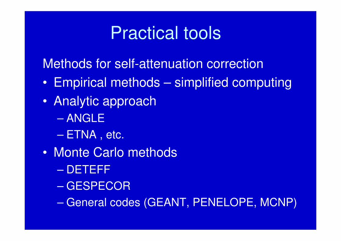
Practical tools

Methods for self-attenuation correction

• Empirical methods – simplified computing

• Analytic approach

– ANGLE

– ETNA , etc.

• Monte Carlo methods

– DETEFF

– GESPECOR

– General codes (GEANT, PENELOPE, MCNP)

Examples

• Importance of the material density

• Influence of the filling height

• Change of matrix

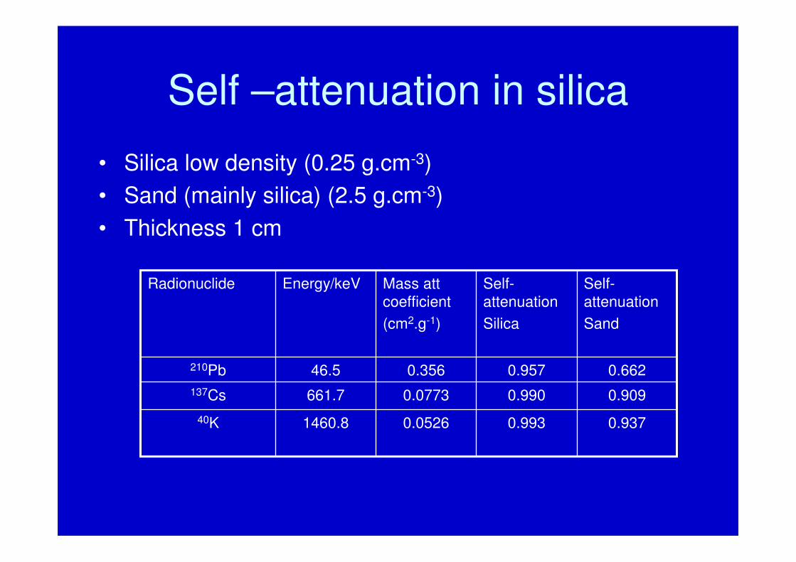
Self –attenuation in silica

• Silica low density (0.25 g.cm-3)

• Sand (mainly silica) (2.5 g.cm-3)

• Thickness 1 cm

0.993

0.990

0.957

Self-

attenuation

Silica

0.6620.35646.5210Pb

0.9090.0773661.7137Cs

0.9370.05261460.840K

Self-

attenuation

Sand

Mass att

coefficient

(cm2.g-1)

Energy/keVRadionuclide

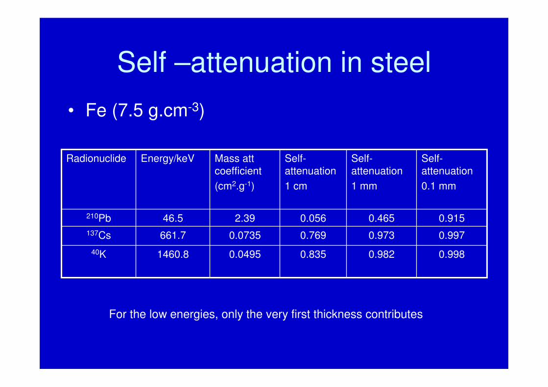
Self –attenuation in steel

• Fe (7.5 g.cm-3)

0.982

0.973

0.465

Self-

attenuation

1 mm

0.835

0.769

0.056

Self-

attenuation

1 cm

0.9152.3946.5210Pb

0.9970.0735661.7137Cs

0.9980.04951460.840K

Self-

attenuation

0.1 mm

Mass att

coefficient

(cm2.g-1)

Energy/keVRadionuclide

For the low energies, only the very first thickness contributes

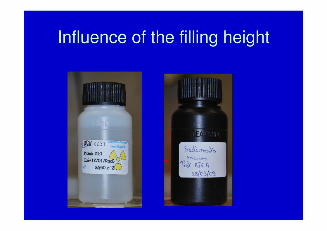
Influence of the filling height

?

Influence of the filling height

0,90

0,95

1,00

1,05

1,10

1,15

1,20

0 500 1000 1500 2000 2500

Filling height = 35 mm

Filling height = 40 mm

Filling height = 43 mm

Filling height = 45 mm

Filling height = 48 mm

Filling height = 50 mm

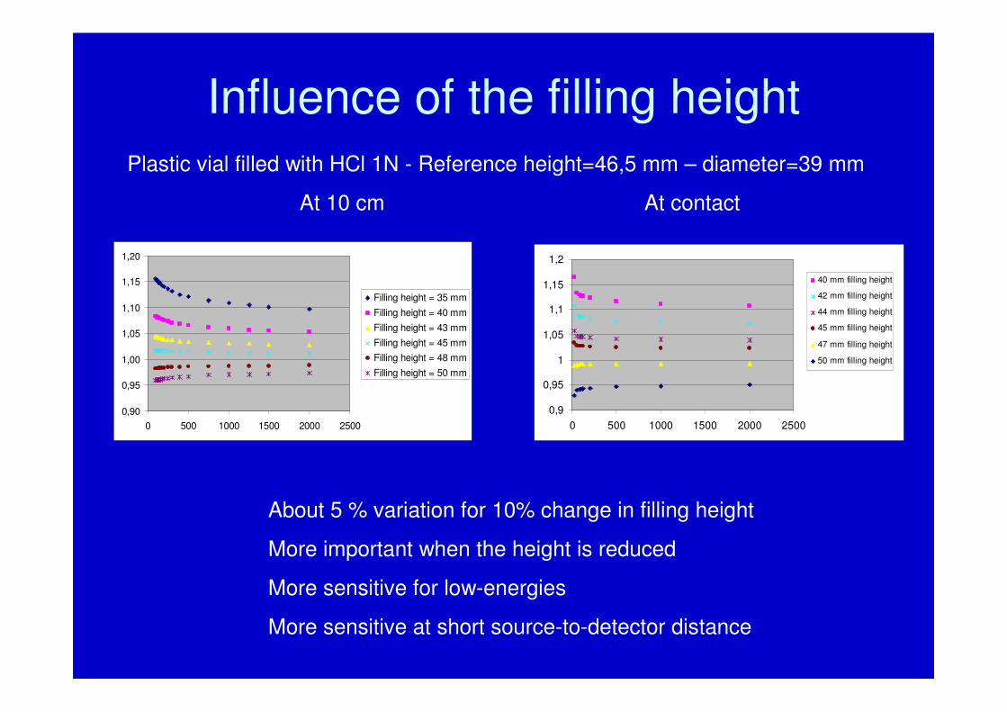
Plastic vial filled with HCl 1N - Reference height=46,5 mm – diameter=39 mm

At 10 cm At contact

0,9

0,95

1

1,05

1,1

1,15

1,2

0 500 1000 1500 2000 2500

40 mm filling height

42 mm filling height

44 mm filling height

45 mm filling height

47 mm filling height

50 mm filling height

About 5 % variation for 10% change in filling height

More important when the height is reduced

More sensitive for low-energies

More sensitive at short source-to-detector distance

Influence of the filling height

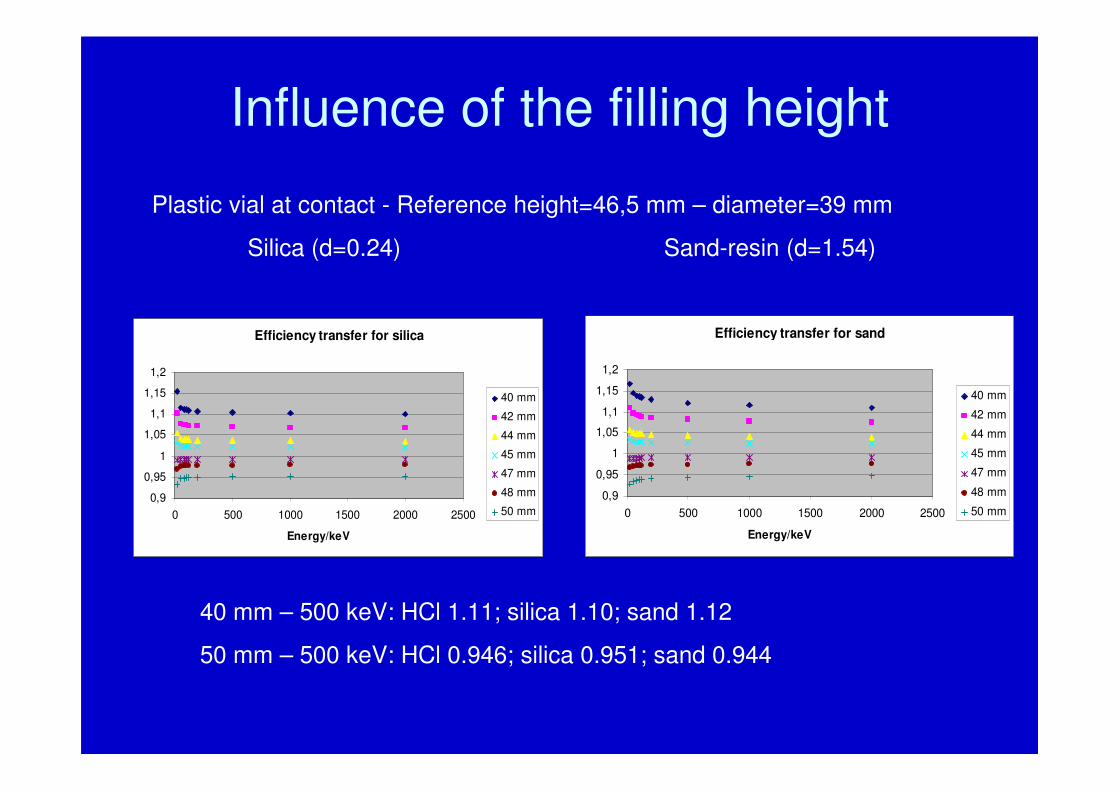
Plastic vial at contact - Reference height=46,5 mm – diameter=39 mm

Silica (d=0.24) Sand-resin (d=1.54)

Efficiency transfer for silica

0,9

0,95

1

1,05

1,1

1,15

1,2

0 500 1000 1500 2000 2500

Energy/keV

40 mm

42 mm

44 mm

45 mm

47 mm

48 mm

50 mm

Efficiency transfer for sand

0,9

0,95

1

1,05

1,1

1,15

1,2

0 500 1000 1500 2000 2500

Energy/keV

40 mm

42 mm

44 mm

45 mm

47 mm

48 mm

50 mm

40 mm – 500 keV: HCl 1.11; silica 1.10; sand 1.12

50 mm – 500 keV: HCl 0.946; silica 0.951; sand 0.944

Influence of the filling height

20 mm +/- 2 mm HCl at contact

0,94

0,96

0,98

1

1,02

1,04

1,06

0 500 1000 1500 2000 2500

Energy/keV

Eff

icie

nc

y t

yra

ns

fer

fac

tor

Filled 22 mm

Filled 18 mm

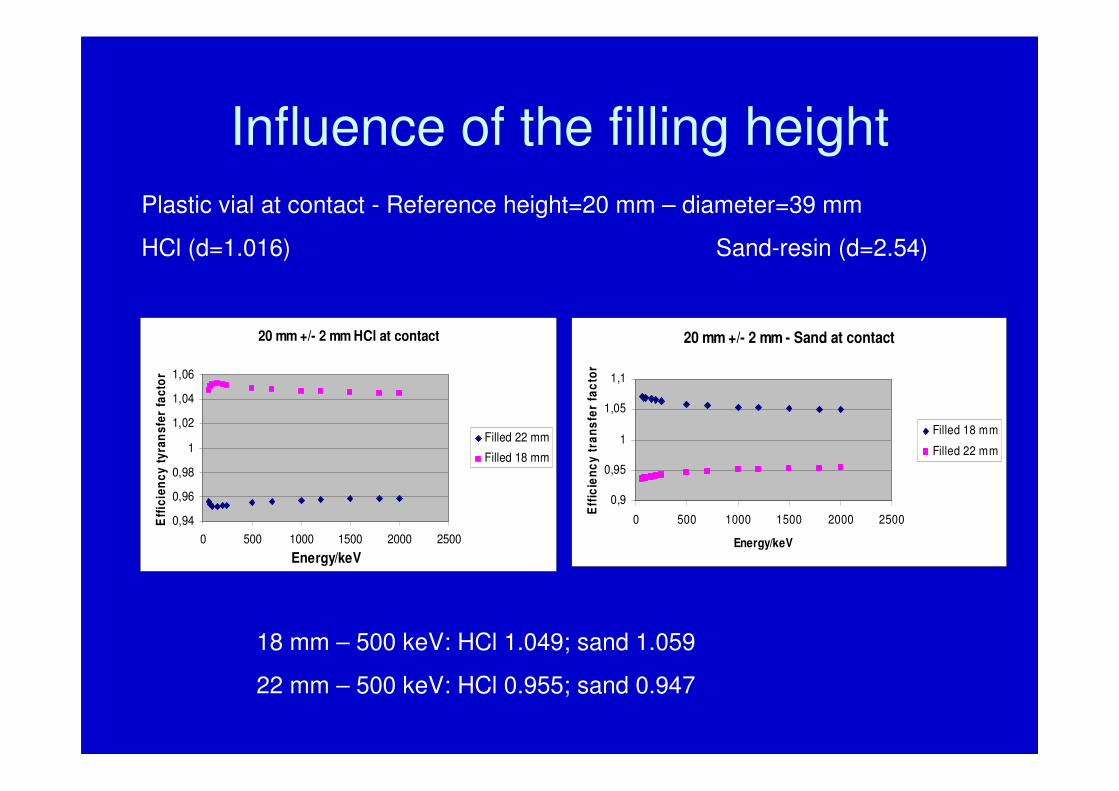
Plastic vial at contact - Reference height=20 mm – diameter=39 mm

HCl (d=1.016) Sand-resin (d=2.54)

20 mm +/- 2 mm - Sand at contact

0,9

0,95

1

1,05

1,1

0 500 1000 1500 2000 2500

Energy/keV

Eff

icie

nc

y t

ran

sfe

r fa

cto

r

Filled 18 mm

Filled 22 mm

18 mm – 500 keV: HCl 1.049; sand 1.059

22 mm – 500 keV: HCl 0.955; sand 0.947

Energie (keV)100 1000

Re

nde

me

nt

0,00

0,02

0,04

0,06

0,08

0,10

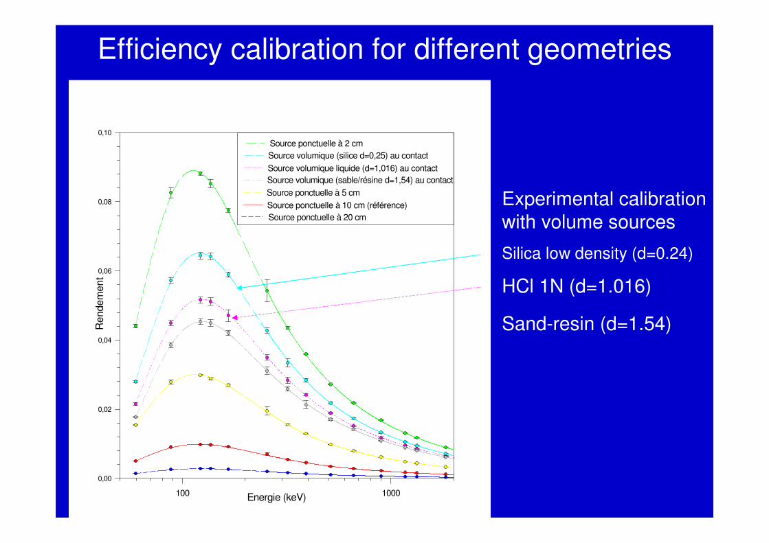
Source ponctuelle à 10 cm (référence)

Source ponctuelle à 2 cm

Source ponctuelle à 5 cm

Source ponctuelle à 20 cm

Source volumique (silice d=0,25) au contact

Source volumique (sable/résine d=1,54) au contact

Source volumique liquide (d=1,016) au contact

Experimental calibration

with volume sources

Silica low density (d=0.24)

HCl 1N (d=1.016)

Sand-resin (d=1.54)

Efficiency calibration for different geometries

Efficiency transfer

Energy

HCl µ Catt

20 0,971 0,219

50 0,225 0,621

80 0,181 0,676

100 0,169 0,693

200 0,137 0,739

500 0,098 0,803

1000 0,072 0,851

2000 0,050 0,892

Silica µ (cm-1) Catt f self

20 0,574 0,349 1,593

50 0,067 0,858 1,383

80 0,043 0,907 1,341

100 0,038 0,917 1,323

200 0,030 0,934 1,264

500 0,021 0,953 1,186

1000 0,015 0,965 1,135

2000 0,011 0,975 1,093

Sand µ (cm-1) Catt f self

20 2,510 0,086 0,391

50 0,385 0,465 0,750

80 0,274 0,565 0,836

100 0,194 0,658 0,950

200 0,199 0,653 0,883

500 0,141 0,733 0,913

1000 0,103 0,794 0,934

2000 0,072 0,849 0,952

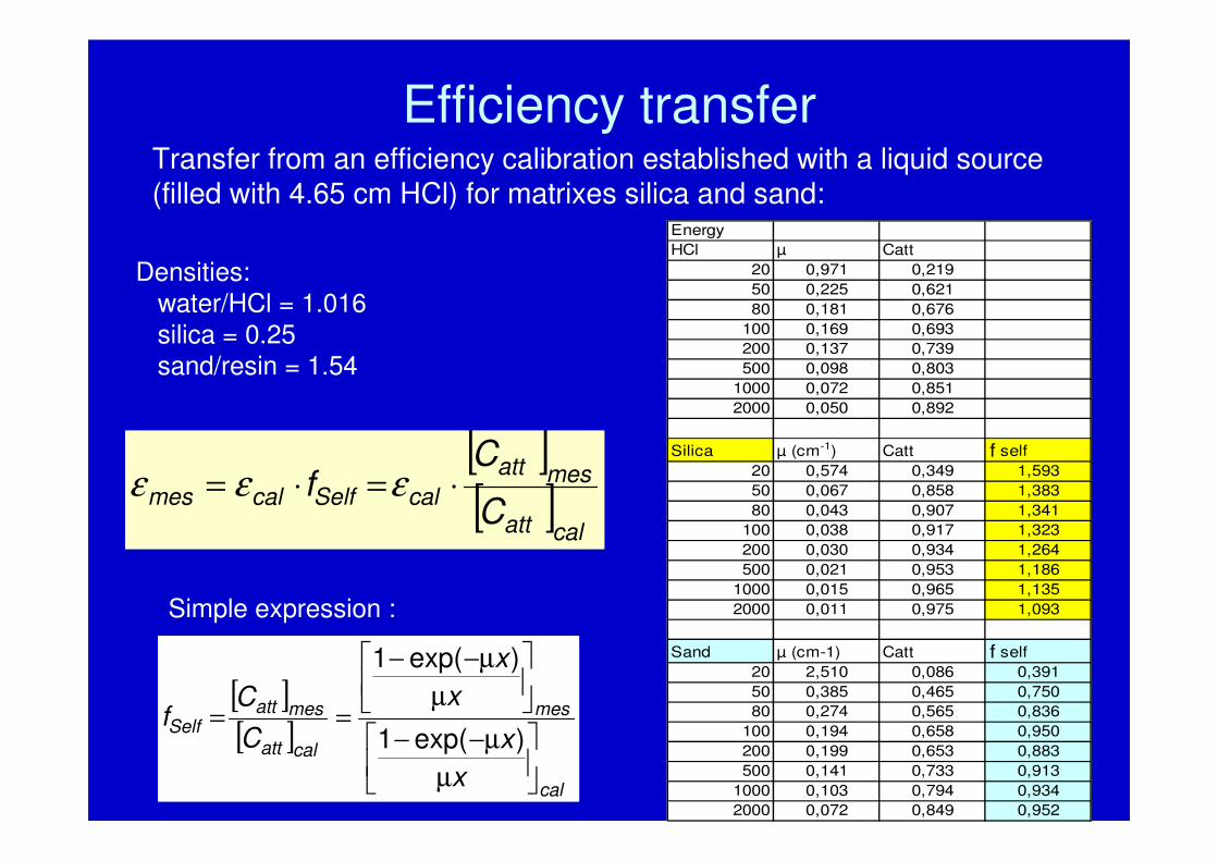
Densities:water/HCl = 1.016silica = 0.25sand/resin = 1.54

[ ][ ]

calatt

mesatt

calSelfcalmesC

Cf ⋅=⋅= εεε

Transfer from an efficiency calibration established with a liquid source (filled with 4.65 cm HCl) for matrixes silica and sand:

Simple expression :

[ ][ ]

cal

mes

calatt

mesattSelf

x

x

x

x

C

Cf

µ

−µ−

µ

−µ−

==)exp(1

)exp(1

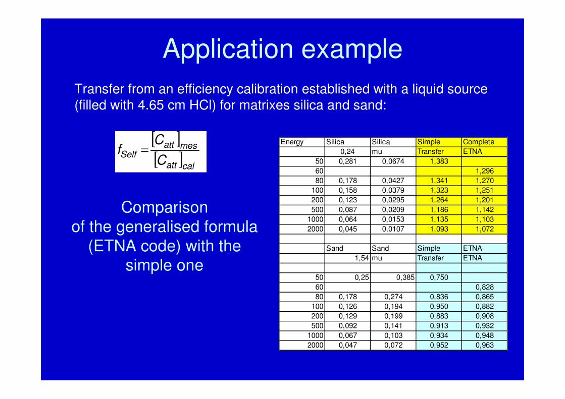
Comparisonof the generalised formula

(ETNA code) with the simple one

Energy Silica Silica Simple Complete

0,24 mu Transfer ETNA

50 0,281 0,0674 1,383

60 1,296

80 0,178 0,0427 1,341 1,270

100 0,158 0,0379 1,323 1,251

200 0,123 0,0295 1,264 1,201

500 0,087 0,0209 1,186 1,142

1000 0,064 0,0153 1,135 1,103

2000 0,045 0,0107 1,093 1,072

Sand Sand Simple ETNA

1,54 mu Transfer ETNA

50 0,25 0,385 0,750

60 0,828

80 0,178 0,274 0,836 0,865

100 0,126 0,194 0,950 0,882

200 0,129 0,199 0,883 0,908

500 0,092 0,141 0,913 0,932

1000 0,067 0,103 0,934 0,948

2000 0,047 0,072 0,952 0,963

Application example

Transfer from an efficiency calibration established with a liquid source (filled with 4.65 cm HCl) for matrixes silica and sand:

[ ][ ]

calatt

mesattSelf

C

Cf =

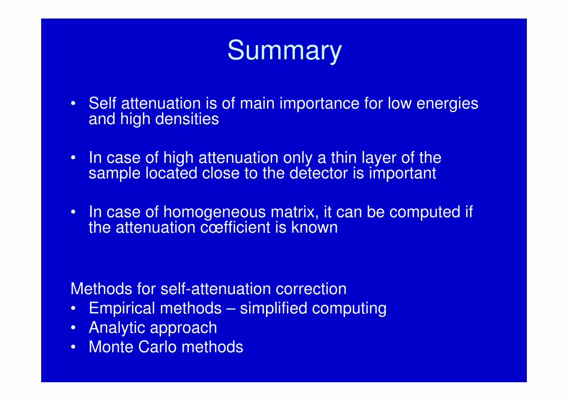
Summary

• Self attenuation is of main importance for low energiesand high densities

• In case of high attenuation only a thin layer of the sample located close to the detector is important

• In case of homogeneous matrix, it can be computed if the attenuation cœfficient is known

Methods for self-attenuation correction• Empirical methods – simplified computing• Analytic approach • Monte Carlo methods