CLOSED SELF-SHRINKING SURFACES

IN R3 VIA THE TORUS

NIELS MARTIN MØLLER

Abstract. We construct many closed, embedded mean curvature self-shrinking sur-faces Σ2

g ⊆ R3 of high genus g = 2k, k ∈ N.Each of these shrinking solitons has isometry group equal to a dihedral group on

2g elements, and comes from the ”gluing”, i.e. desingularizing the singular union,of the two known closed embedded self-shrinkers in R3: The round 2-sphere S2, andAngenent’s self-shrinking 2-torus of revolution T2. This uses the results and methodsN. Kapouleas developed for minimal surfaces in [Ka97]–[Ka].

1. Introduction

Recall that a smooth surface Σ2 ⊆ R3 is a mean curvature self-shrinker if it satisfiesthe corresponding nonlinear elliptic self-shrinking soliton PDE:

(1.1) H(Σ) =〈X, νΣ〉

2, X ∈ Σ2 ⊆ R3,

where H denotes the mean curvature, X the position vector and νΣ is a unit lengthvector field normal to Σ2 ⊆ R3.

While important as singularity models in mean curvature flow (see e.g. [Hu90]-[Hu93]and [CM6]-[CM8]), the list of known closed, embedded surfaces satisfying Equation(1.1) is short:q The round 2-sphere S2 ⊆ R3,q Angenent’s (non-circular) 2-torus, in [An92].

Apart from these, there is numerical evidence for the existence of a self-shrinking”fattened wire cube” in [Ch94], and in higher dimensions there are Lagrangian examples(generalizing the Abresch-Langer curves [AL86]), found by Anciaux in [Anc06].

One can rigorously construct closed, embedded, smooth mean curvature self-shrinkerswith high genus g, embedded in Euclidean space R3:

Theorem 1. For every large enough even integer g = 2k, k ∈ N, there exists a compact,embedded, orientable, smooth surface without boundary Σ2

g ⊆ R3, with the properties:

(i) Σg is a mean curvature self-shrinker of genus g.(ii) Σg is invariant under the dihedral symmetry group with 2g = 4k elements.

Date: September 29, 2014.Key words and phrases. Mean curvature flow, self-shrinkers, self-similarity, solitons, minimal sur-

faces, gluing constructions, stability theory, geodesics, spectral theory.The author was supported partially by NSF award DMS-1311795.

1

arX

iv:1

111.

7318

v2 [

mat

h.D

G]

18

Nov

201

4

(iii) The sequence {Σg} converges in Hausdorff sense to the union S2 ∪ T2, whereT2 is a rotationally symmetric self-shrinking torus in R3. The convergence islocally smooth away from the two intersection circles constituting S2 ∩ T2.

This paper consists of: (1) Brief account of the construction and its importantcomponents, and (2) Proofs of the central explicit estimates of functions that for somesmall δ, ε > 0 in an appropriate sense are δ-close to being eigenfunctions of the stabilityoperator (corresp. δ-Jacobi fields), on surfaces that are ε-close to being self-shrinkers(corresp. ε-geodesics) near a candidate for the self-shrinking torus.

The implications of such estimates are: The existence of a self-shrinking torus T2

(via existence of a smooth closed geodesic loop) with useful quantitative estimates ofits geometry. Hence it gives conclusions about the Dirichlet and Neumann problemsof the stability operator L on this ”quantitative torus”, leading to the main technicalresult below in Theorem 2.7 which is sufficient to prove Theorem 1.

A thorough treatment of the background and details relating to this problem, and theconstruction as developed for general compact minimal hypersurfaces in 3-manifolds byNikolaos Kapouleas in [Ka97]-[Ka05] can be found in the recent [Ka11], the contents ofwhich will not be described here (it should be noted that the highly symmetric specialcase enjoys significant simplifications compared to the full theory). Note that also thereferences [Ng06]-[Ng07], and more recently [KKMø] and [Ng11], were concerned withgluing problems for (non-compact) self-shrinkers.

Self-shrinkers are minimal surfaces in Euclidean space with respect to a conformallychanged Gaussian metric g:

(1.2)

Σn ⊆ Rn+1 is a self-shrinker ⇐⇒ H(Rn+1,g)(Σ) = 0,

gij =δij

exp (|X|2/2n), X ∈ Rn+1.

Recall the constructions by Nicos Kapouleas (in [Ka97]-[Ka11]), concerning desin-gularization of a finite collection of compact minimal surfaces in a general ambientRiemannian 3-manifold (M3, g). The conditions for the construction to work, in oursituation, are the following, where the collection is identified with one immersed surfaceW with intersections along the (smooth) curve C, which can have several connectedcomponents.

Conditions 1.1 ([Ka05]-[Ka11]).(I) There are no points of triple intersection, all intersections are transverse andC ∩ ∂W = ∅ holds.

(N1) The kernel for the linearized operator

(1.3) L = ∆ + |A|2 + Ric(ν, ν) on W,

with Dirichlet conditions on ∂W, is trivial (unbalancing condition).

(N2) The kernel for the linearized operator L on W, with Dirichlet conditions on

∂W, is trivial (flexibility condition).

Instead of (N1) one may substitute:

(N1’) The kernel for the linearized operator L on W, with Neumann conditions on∂W, is trivial (unbalancing condition).

2

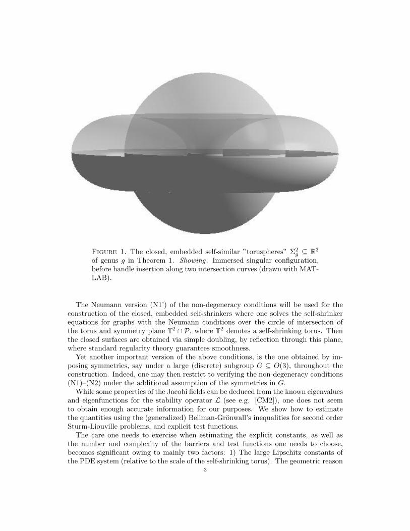
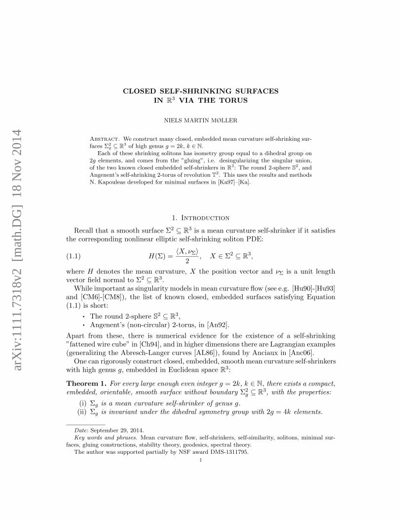
Figure 1. The closed, embedded self-similar ”toruspheres” Σ2g ⊆ R3

of genus g in Theorem 1. Showing : Immersed singular configuration,before handle insertion along two intersection curves (drawn with MAT-LAB).

The Neumann version (N1’) of the non-degeneracy conditions will be used for theconstruction of the closed, embedded self-shrinkers where one solves the self-shrinkerequations for graphs with the Neumann conditions over the circle of intersection ofthe torus and symmetry plane T2 ∩ P, where T2 denotes a self-shrinking torus. Thenthe closed surfaces are obtained via simple doubling, by reflection through this plane,where standard regularity theory guarantees smoothness.

Yet another important version of the above conditions, is the one obtained by im-posing symmetries, say under a large (discrete) subgroup G ⊆ O(3), throughout theconstruction. Indeed, one may then restrict to verifying the non-degeneracy conditions(N1)–(N2) under the additional assumption of the symmetries in G.

While some properties of the Jacobi fields can be deduced from the known eigenvaluesand eigenfunctions for the stability operator L (see e.g. [CM2]), one does not seemto obtain enough accurate information for our purposes. We show how to estimatethe quantities using the (generalized) Bellman-Gronwall’s inequalities for second orderSturm-Liouville problems, and explicit test functions.

The care one needs to exercise when estimating the explicit constants, as well asthe number and complexity of the barriers and test functions one needs to choose,becomes significant owing to mainly two factors: 1) The large Lipschitz constants ofthe PDE system (relative to the scale of the self-shrinking torus). The geometric reason

3

that this happens is that the Gauß curvature in the metric on Angenent’s upper half-plane has a maximal value of around 30 along the candidate torus (with the maximumoccurring at the point nearest to the origin in R3), giving naive characteristic conjugatedistances of down to π√

K∼ 0.5, while the circumference of the torus is around ∼ 7, in

the metric. Hence the solutions to Jacobi’s equation can be expected to, and indeeddo, oscillate several times around the circumference of T2, in a non-uniform way andyet just fall short of ”matching up” smoothly. Furthermore: 2) The location of theconjugate points on S2 for the appropriate Jacobi equation is very near the singularcurve C (i.e. the boundaries of the connected components ofM\C), which also requirestighter estimates.

Hence it takes work to strengthen the estimates to a useful form. One device todo this is what could be called the ”sesqui”-shooting problem in Definition 2.4, foridentifying the position of the torus, where ”sesqui” refers to the fact that it is a doubleshooting problem but with a compatibility condition linking the two: That each pairof curves always meet at a simple, explicitly known solution. Here we take the roundcylinder of radius

√2 as reference. Since the errors are exponential in the integral

of the Lipschitz constants, one may by virtue of the sesqui-shooting roughly take thesquare-root of the errors, which allows us to obtain bounds with explicit constants ofthe order of 101–102 instead of 104.

Although reduced in volume by the above discussion, it turns out that the explicitchoice of test functions (f.ex. adequate piecewise polynomial choices can easily be foundusing a Taylor expansion fit at selected points, deduced from a numerical solution tothe PDEs), to insert into the key estimates in Section 2, still take up several pages,and is not in itself very enlightening material to include. The computational job ofchecking the estimates for the many low-degree polynomials is in any case best carriedout using computer software. The corresponding figures throughout this paper, showingAngenent’s torus and the relevant Jacobi fields, were likewise computed and drawn inMATLAB.

Thus, the present paper does not contain the most efficient result that one couldhope for, by amounting in effect to the reduction of the rigorous proof of the existenceof closed self-shrinkers with genus to the still non-trivial algorithmic task of findingthe zeros of several explicit low-order polynomials with integer coefficients (of course atask a computer easily manages rigorously).

2. ε-Geodesics, δ-Jacobi Fields: A Quantitative Self-Shrinking Torus T2

2.1. Existence of T2, With Geometric Estimates. In order to later understandprecisely the kernel of the stability operators, we need to establish a detailed quan-titative version of the existence of Angenent’s torus. Towards the end of this sectionwe will arrive at the basic, explicit estimates on the location and geometric quantitiesof such a torus, but we will first work out the explicit estimates for also the Jacobiequation before finalizing the choices in the estimate, in order to require as little aspossible of the test functions.

We note that much less complicated estimates (and ditto test functions) would en-sure the mere existence, leading to a different proof of the self-shrinking ”doughnut”

4

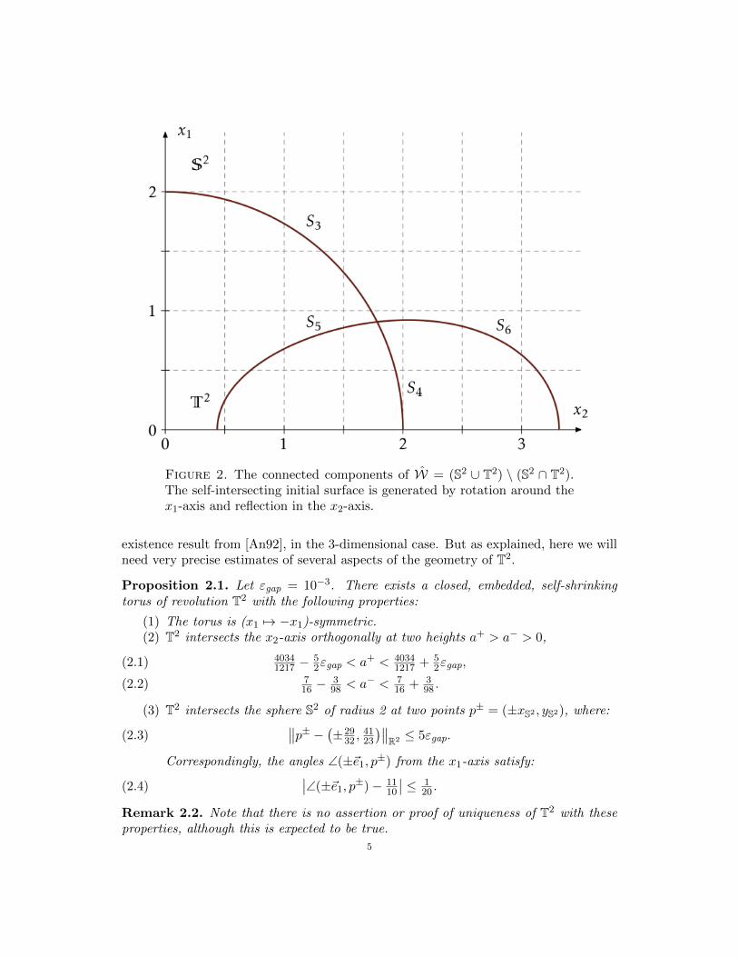
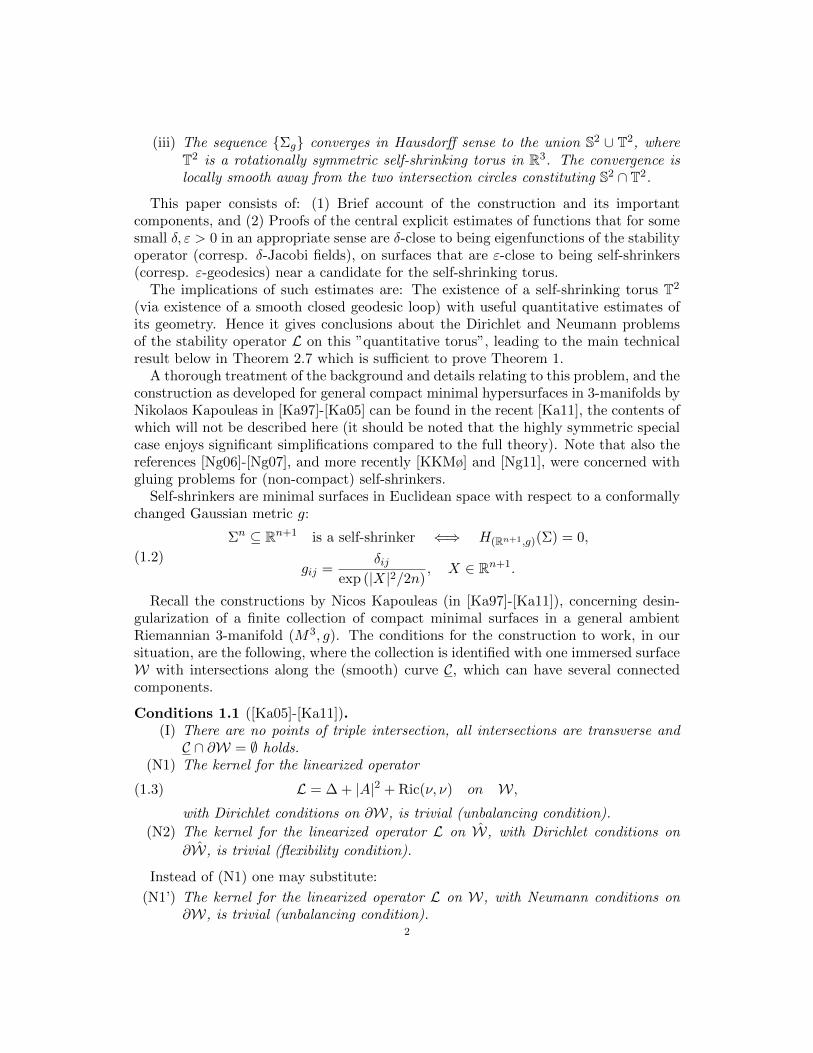
Figure 2. The connected components of W = (S2 ∪ T2) \ (S2 ∩ T2).The self-intersecting initial surface is generated by rotation around thex1-axis and reflection in the x2-axis.

existence result from [An92], in the 3-dimensional case. But as explained, here we willneed very precise estimates of several aspects of the geometry of T2.

Proposition 2.1. Let εgap = 10−3. There exists a closed, embedded, self-shrinkingtorus of revolution T2 with the following properties:

(1) The torus is (x1 7→ −x1)-symmetric.(2) T2 intersects the x2-axis orthogonally at two heights a+ > a− > 0,

40341217 −

52εgap < a+ < 4034

1217 + 52εgap,(2.1)

716 −

398 < a− < 7

16 + 398 .(2.2)

(3) T2 intersects the sphere S2 of radius 2 at two points p± = (±xS2 , yS2), where:∥∥p± − (±2932 ,

4123

)∥∥R2 ≤ 5εgap.(2.3)

Correspondingly, the angles ∠(±~e1, p±) from the x1-axis satisfy:

(2.4)∣∣∠(±~e1, p

±)− 1110

∣∣ ≤ 120 .

Remark 2.2. Note that there is no assertion or proof of uniqueness of T2 with theseproperties, although this is expected to be true.

5

Proof. We first need to describe the double shooting problem (or rather ”sesqui”-shooting problem, since we remove one parameter). For this we need an elementarylemma, which can either be proved (in a weaker version) using the approximationmethods described later in this section, or by analysis directly of the ODE in (2.32).

Lemma 2.3. For each d ∈ [0,√

2] let γd : [0,∞)→ R+ ×R be the geodesic starting at(0, d) with initial derivative γ′d(0) = (1, 0) and consider the first time t0(d) such that

γd intersects the cylinder geodesic {x2 =√

2}. Then the function I : [0,√

2] → [0,√

2]given by

I(d) := x1(γs(t0(d))),

is continuous and strictly increasing. It satisfies the bounds:

1 ≤ supd∈[ 13

32,1532

]

I ′(d) ≤ 5

4.

Definition 2.4 (”Sesqui”-Shooting Problem).(i) Fix a >

√2.

(ii) Let γa : [0, ta] → R+ × R be the fully extended geodesic contained in {x1 ≥ 0},with initial conditions γa(0) = (0, a) and γ′a(0) = (1, 0).

(iii) By the maximum principle for (2.32), we have γa ∩ {x2 =√

2} 6= ∅. Assumethat the first point of γa crossing

√2 belongs to {0 < x1 ≤

√2}, and denote the

time it happens by t0(a).(iv) By the preceding Lemma, there exists a unique b(a) ∈ [0,

√2] and s0(a) such

that for γb on [0, s0] with γb(0) = (0, b) and γ′b(0) = (1, 0), we have

γa(t0(a)) = γb(s

0(a)).

(iv) Define Φ(a) by

Φ(a) :=~e3 · (γ′a(t0(a))× γ′b(s0(a))

|γ′a(t0(a))||γ′b(s0(a))|,

or equivalently the oriented angle between the tangents of γa and γb at theintersection point.

The following lemma is clear from the definition:

Lemma 2.5. The function Φ in Definition 2.4 is well-defined and continuous, on theopen connected set of values a >

√2 with the property that the first point of intersection

of γa with {x2 =√

2} belongs to {x1 ∈ (0,√

2)}.

The strategy for the proof of the proposition will now be to prove for two differentnearby pairs (a+, b+) and (a−, b−), that will be chosen such that they are geodesicsbroken at the cylinder {x2 =

√2}, that:

Φ(a+) > 0,(2.5)

Φ(a−) < 0.(2.6)

6

Existence then follows, from the intermediate value theorem, of a pair (a0, b0) suchthat:

Φ(a0) = 0,(2.7)

a− < a0 < a+,(2.8)

b− < b0 < b+.(2.9)

The estimates leading to the proof of (2.5)–(2.6) will then lead to the estimates in theproposition.

Consider now a curve (parametrized by any parameter t),

γ(t) = (x(t), y(t)).

Then the equation for γ to generate a self-shrinker by rotation reads:

x′′y′ − y′′x′ =[yx′ − xy′

2− x′

y

] ((x′)2 + (y′)2

).

We need the following simple lemma:

Lemma 2.6. If we define the operatorM1 acting on C2-functions u : I → R, for someinterval I ⊆ [0,∞], by

(2.10) M1(u, p) :=[x1p− u

2+

1

u

](1 + p2

),

then the function u(x1), a graph over the x1-axis, generates a self-shrinker by rotation(around x1) if and only if

(2.11) u′′ =M1(u, u′).

Likewise for graphs over the x2-axis, defining

(2.12) M2(f, q) :=

[(x2

2− 1

x2

)q − f

2

] (1 + q2

),

again characterizes such solutions via

(2.13) f ′′ =M2(f, f ′).

The lemma is shown directly from the definition of a self-shrinker (see [KMø]). Wenow compute that:

∂

∂uM1(u, p) =

[−1

2− 1

u2

](1 + p2),(2.14)

∂

∂pM1(u, p) =

x1

2(1 + p2) + 2p

[x1p− u

2+

1

u

],(2.15)

∂

∂fM2(f, q) = −1

2

(1 + q2

),(2.16)

∂

∂qM2(f, q) =

(x2

2− 1

x2

)(1 + 3q2)− fq.(2.17)

We will first consider graphs u : [0, 35 ] → R. Now, considering an approximate

solution U , fix the quantity εT1 , later to be chosen, which reflects the order of magnitudeof the precision with which we wish to determine the position of T2 on this interval.

7

(2.18) M1(U,U ′)−M1(u, u′) = (U − u)∂

∂uM1(ξ, u′) + (U ′ − u′) ∂

∂pM1(U, ξ′),

for some ξ ∈ [U(x1), u(x1)] and ξ′ ∈ [U ′(x1), u′(x1)].Top of the torus: x1-graphAssume we have the uniform estimates:

|U ′′ −M1(U,U ′)| ≤ εT1 ,

for some εT1 . Assume also the following bounds:∫ x1

0

∣∣∣∣12 +1

ξ2

∣∣∣∣ (1 + (u′(x1))2)dx1 ≤4

5x1, x1 ∈ [0, 3

5 ], |ξ − U(x1)| ≤ ε0,∫ x1

0

∣∣∣∣x1

2(1 + (ξ′)2) + 2ξ′

[x1ξ′ − U(x1)

2+

1

U(x1)

]∣∣∣∣ dx1 ≤8

3x2

1, x1 ∈ [0, 35 ], |ξ′ − U ′(x1)| ≤ ε0.

If we let ϕ(x1) := |U ′(x1)−u′(x1)|, we can now estimate (recall that one has ||f ′|′| = |f ′′|almost everywhere):

ϕ′(x1) ≤∣∣|U ′ − u′|′∣∣ a.e

= |U ′′ − u′′|≤ |M1(U,U ′)−M1(u, u′)|+ εT1

≤ |∂uM1(ξ, u′)||U − u|+ |∂pM1(U, ξ′)||U ′ − u′|+ εT1

≤ |∂pM1(U, ξ′)|ϕ(x1) + |∂uM1(ξ, u′)|∫ x1

0ϕ(s)ds+ |∂uM1(ξ, u′)||U(0)− u(0)|+ εT1 .

(2.19)

Thus we integrate this inequality, which holds almost everywhere with respect to theLebesgue measure, and get:

ϕ(x1) ≤ ϕ(0) +

∫ x1

0|∂pM1(U, ξ′)(s)|ϕ(s)ds+

∫ x1

0|∂uM1(ξ, u′)(t)|

∫ t

0ϕ(s)dsdt

+ 45x1|U(0)− u(0)|+ εT1 x1

≤ ϕ(0) + 45x1|U(0)− u(0)|+ εT1 x1 +

∫ x1

0

[|∂pM1(U, ξ′)(s)|+ 4

5x1

]ϕ(s)ds.

We are now ready to use the integral form of Gronwall-Bellman’s inequality, namelyfor α(t) a non-decreasing function:

∀t ∈ I : ϕ(t) ≤ α(t) +

∫ t

aβ(s)ϕ(s)ds =⇒ ∀t ∈ I : ϕ(t) ≤ α(t) exp

{∫ t

aβ(s)ds

}.

Here we thus conclude from the above, that

(2.20) ϕ(x1) ≤[ϕ(0) + 4

5x1|U(0)− u(0)|+ εT1 x1

]exp

{83x

21 + 4

5x21

},

8

so that here we obtain the estimates (for ϕ(0) = 0):

|U ′(x1)− u′(x1)| ≤ 35 exp(156

125)(εT1 + 45 |U(0)− u(0)|),

|U(x1)− u(x1)| ≤ |U(0)− u(0)|+ (εT1 + 45 |U(0)− u(0)|)

∫ 35

0s exp

(5215s

2)ds

= |U(0)− u(0)|+ 15104

(exp

(5215(3

5)2)− 1)(εT1 + 4

5 |U(0)− u(0)|)≤ 23

80 |U(0)− u(0)|+ 925ε

T1 .

Top of the torus: x2-graph to the sphereWe continue with the next part, which is graphical over the x2-axis. In this region

we again let ψ(x2) := |F ′ − f ′|. Here we will assume the estimate

(2.21) |F ′′ −M2(F, F ′)| ≤ εT2 ,

and furthermore the estimates on x2 ∈ [yS2 , uT (3/5)]

I(2)u =

∫ uT (3/5)

x2

∣∣∣∣12(1 + (F ′)2)

∣∣∣∣ dx2 ≤ 138 −

x22 ,

I(2)p =

∫ uT (3/5)

x2

∣∣∣∣(x2

2− 1

x2

)(1 + 3(ξ′)2)− F (x2)ξ′

∣∣∣∣ dx2 ≤ 74 −

910 (x2 − yS2)2 .

We can then estimate as follows:

ψ′(x2) ≤ |∂uM2| |F − f |+ |∂pM2| |F ′ − f ′|+ εT2

≤ |∂uM2|∫ a

x2

ψ(s)ds+ |∂pM2|ψ(x2) + |∂uM2| |F (a)− f(a)|+ εT2 ,

which integrates to

ψ(x2) ≤∫ uT (3/5)

x2

[|∂pM2|+ 13

8 −x22

]ψ(s)ds+ (13

8 −x22 )|F (uT (3/5))− f(uT (3/5))|

(2.22)

+ εT2 (uT (3/5)− x2) + ψ(a),(2.23)

so that, again by Gronwall-Bellman,

ψ(x2) ≤[(13

8 −x22 )|F (a)− f(a)|+ |F ′(a)− f ′(a)|+ εT2 (uT (3/5)− x2)

]×

exp{

74 −

910 (x2 − yS2)2 +

(138 −

x22

)(uT (3/5)− x2)

}.

The endpoint estimates for |F ′(x2)− f ′(x2)| are thus:

ψ(yS2) ≤ 594 |F (uT (3/5))− f(uT (3/5))|+ 54

5 |F′(uT (3/5))− f ′(uT (3/5))|+ 377

20 εT2

≤ 594

|U(F (uT (3/5)))− u(f(uT (3/5)))||U ′(F (ξ))|

+ 545

|U ′(F (uT (3/5)))− u′(f(uT (3/5)))||U ′(F (uT (3/5)))||u′(f(uT (3/5)))|

+ 37720 ε

T2

≤ 594

1011

(925ε

T1 + 23

80 |U(0)− u(0)|)

+ 545

(1011

)2 35 exp(156

125)(εT1 + 45 |U(0)− u(0)|) + 377

20 εT2

≤ 27|U(0)− u(0)|+ 34εT1 + 19εT2 .9

Integrating the above estimate for ψ(x2), we also get:

|F (yS2)− f(yS2)| ≤(1 + 638 )|F (uT (3/5))− f(uT (3/5))|+ 83

20 |F′(uT (3/5))− f ′(uT (3/5))|+ 137

20 εT2

≤12|U(0)− u(0)|+ 15εT1 + 7εT2 .

Top of the torus, x2-graph from sphere to cylinderWe consider the region between the sphere and cylinder, and let again ψ(x2) :=

|F ′ − f ′|. Here we will assume the estimate

(2.24) |F ′′ −M2(F, F ′)| ≤ εT3 ,

and furthermore the estimates on x2 ∈ [yS2 ,√

2]

I(2)u =

∫ yS2

x2

∣∣∣∣12(1 + (F ′)2)

∣∣∣∣ dx2 ≤ 14(yS2 − x2),

I(2)p =

∫ yS2

x2

∣∣∣∣(x2

2− 1

x2

)(1 + 3(ξ′)2)− F (x2)ξ′

∣∣∣∣ dx2 ≤ 2750(yS2 − x2).

We estimate as follows:

ψ′(x2) ≤ |∂uM2| |F − f |+ |∂pM2| |F ′ − f ′|+ εT2

≤ |∂uM2|∫ yS2

x2

ψ(s)ds+ |∂pM2|ψ(x2) + |∂uM2| |F (yS2)− f(yS2)|+ εT3 ,

which integrates to:

ψ(x2) ≤ψ(yS2) +

∫ yS2

x2

[|∂pM2|+ 1

4(yS2 − x2)]ψ(s)ds+ 1

4(yS2 − x2)|F (yS2)− f(yS2)|+ εT3 (yS2 − x2),

(2.25)

so that, again by Gronwall-Bellman,

ψ(x2) ≤[

14(yS2 − x2)|F (yS2)− f(yS2)|+ |F ′(yS2)− f ′(yS2)|+ εT3 (yS2 − x2)

]×

exp{

2750(yS2 − x2) + 1

4(yS2 − x2)2}.

Inserting the previous estimate gives:

ψ(√

2) ≤ 18 |F (yS2)− f(yS2)|+ 4

3 |F′(yS2)− f ′(yS2)|+ 1

2εT3

≤ 18

(12|U(0)− u(0)|+ 15εT1 + 7εT2

)+ 4

3

(27|U(0)− u(0)|+ 34εT1 + 19εT2

)+ 1

2εT3 .

Hence, we finally obtain the estimate:

|F ′(√

2)− f ′(√

2)| ≤ 36|U(0)− u(0)|+ 45εT1 + 25εT2 + 12εT3 .

Integrating the estimates, we also get:

|F (yS2)− f(yS2)| ≤(1 + 150)|F (yS2)− f(yS2)|+ 33

80 |F′(yS2)− f ′(yS2)|+ 2

25εT3

≤24|U(0)− u(0)|+ 30εT1 + 15εT2 + 225ε

T3 .

Bottom of the torus: x1-graph from the planeAssume uniform estimates:

|U ′′ −M1(U,U ′)| ≤ εB1 ,10

for some εB1 . Assume also, for the argument, the following bounds (for x1 ∈ [0, 12 ]):∫ x1

0

∣∣∣∣12 +1

ξ2

∣∣∣∣ (1 + (u′(x1))2)dx1 ≤29

5x1 +

1

20, |ξ − U(x1)| ≤ ε0,∫ x1

0

∣∣∣∣x1

2(1 + (ξ′)2) + 2ξ′

[x1ξ′ − U(x1)

2+

1

U(x1)

]∣∣∣∣ dx1 ≤ 4x21 +

1

5x1, |ξ′ − U ′(x1)| ≤ ε0.

As always, we get with ϕ(x) = |U ′(x)− u′(x)|:

ϕ(x1) ≤ ϕ(0) +

∫ x1

0|∂pM1(U, ξ′)(s)|ϕ(s)ds+

∫ x1

0|∂uM1(ξ, u′)(t)|

∫ t

0ϕ(s)dsdt

+ (295 x1 + 1

20)|U(0)− u(0)|+ εB1 x1

≤ ϕ(0) + (295 x1 + 1

20)|U(0)− u(0)|+ εB1 x1 +

∫ x1

0

[|∂pM1(U, ξ′)(s)|+ 29

5 x1 + 120

]ϕ(s)ds.

Using once again Gronwall-Bellman’s inequality,

(2.26) ϕ(x1) ≤[ϕ(0) + (29

5 x1 + 120)|U(0)−u(0)|+εB1 x1

]exp

{295 x

21 + x1

20 + 4x21 + 1

5x1

},

and we obtain the estimates (for ϕ(0) = 0):

|U ′(x1)− u′(x1)| ≤[(29

5 x1 + 120)|U(0)− u(0)|+ εB1 x1

]exp

{495 x

21 + x1

4

}|U ′(1

2)− u′(12)| ≤ 39|U(0)− u(0)|+ 28

5 εB1 ,

|U(x1)− u(x1)| ≤ |U(0)− u(0)|(

1 +

∫ x1

0(29

5 s+ 120) exp

{495 s

2 + s4

}ds

)+ εB1

∫ x1

0s exp

{495 s

2 + s4

}ds

|U(12)− u(1

2)| ≤ 235 |U(0)− u(0)|+ 3

5εB1 .

Bottom: x2-graph to cylinderWe continue with the next part, which is graphical over the x2-axis. In this region

we again let ψ(x2) = ψB(x2) := |F ′ − f ′|. Here we will assume the estimate

(2.27) |F ′′ −M2(F, F ′)| ≤ εB2 ,

and furthermore the estimates on x2 ∈ [a0,√

2] (where |a0 − 2839 | ≤ ε0).

I(2)u =

∫ x2

a0

∣∣∣∣12(1 + (F ′)2)

∣∣∣∣ dx2 ≤16

25x2 −

3

7,

I(2)p =

∫ x2

a0

∣∣∣∣(x2

2− 1

x2

)(1 + 3(ξ′)2)− F (x2)ξ′

∣∣∣∣ dx2 ≤9

10− 11

10

(x2 −

3

2

)2

.

We can then estimate as follows:

ψ′(x2) ≤ |∂uM2| |F − f |+ |∂pM2| |F ′ − f ′|+ εB2

≤ |∂uM2|∫ x2

aψ(s)ds+ |∂pM2|ψ(x2) + |∂uM2| |F (a)− f(a)|+ εB2 ,

11

which integrates to

ψ(x2) ≤∫ x2

a0

[|∂pM2|+ 16

25x2 − 37

]ψ(s)ds+ (16

25x2 − 37)|F (a0)− f(a0)|+ εB2 (x2 − a0) + ψ(a).

(2.28)

By Gronwall-Bellman,

ψ(x2) ≤[(16

25x2 − 37)|F (a)− f(a)|+ |F ′(a)− f ′(a)|+ εB2 (x2 − a0)

]×

exp{

910 −

1110

(x2 − 3

2

)2+ (x2 − a0)

(1625x2 − 3

7

)}≤ 13

8 |F (a0)− f(a0)|+ 175 |F

′(a0)− f ′(a0)|+ 6929ε

B2

≤ 138

|U(F (a0))− u(f(a0))||U ′(F (ξ))|

+ 175

|U ′(F (a0))− u′(f(a0))||U ′(F (a0))||u′(f(a0))|

+ 6929ε

B2

≤ 138

1012

(35εB1 + 23

5 |U(0)− u(0)|)

+ 175

(1012

)2(28

5 εB1 + 39|U(0)− u(0)|) + 69

29εB2

≤ 100|U(0)− u(0)|+ 15εB1 + 52εB2 .

Integrating the first line of this estimate, we also get:

|F (√

2)− f(√

2)| ≤(1 + 2350)|F (a0)− f(a0)|+ 14

9 |F′(a0)− f ′(a0)|+ 2

3ε2

≤48|U(0)− u(0)|+ 7εB1 + 23εB2 .

Hence one arranges that for the test functions γup, γlow : [0, 1]→ R× R+:

γdown(0) = (0, 40341217 −

52εud)(2.29)

γup(0) = (0, 40341217 + 5

2εud).(2.30)

Then, as explained earlier, the intermediate value theorem applied to the sesqui-shooting problem implies the existence of the torus with the estimates (2.1)–(2.2).

To see Property (3), we recall that

(2.31) |F (yS2)− f(yS2)| ≤ 31725 |U(0)− u(0)|+ 11ε1 + 27

5 ε2,

from which the estimate (2.3) follows.�

2.2. The Stability Operator L on Subsets of S2 and T2. Recall the self-shrinkerequation for a smooth oriented surface S ⊆ R3 to be a self-shrinker (shrinking towardsthe origin with singular time T = 1) is

(2.32) HS( ~X)− 12~X · ~νS( ~X) = 0,

for each ~X ∈ S, where by convention HS =∑n

1 κi is the sum of the signed principalcurvatures w.r.t. the chosen normal ~νS (i.e. H = 2 for the sphere with outward pointing~ν). We have normalized Equation (2.32) so that T = 1 is the singular time.

For a smooth normal variation ~Xt determined by a function u via Xt = X0 + tu~νS ,

where ~X0 parametrizes S, the pointwise linear change in (minus) the quantity on the12

left hand side in (2.32) is given by the stability operator (see the Appendix, and also[CM6]-[CM7] for more properties of this operator)

(2.33) LSu = ∆Su+ |AS |2u− 12

(~X · ∇Su− u

).

We are now ready to prove the main technical theorem in this paper, concerning thekernel on the connected components (with boundaries) of

(S2 ∪ T2) \ (S2 ∩ T2),

where T2 is the accurately estimated ”quantitative” torus.

Theorem 2.7. There exists N > 0 large enough that for the below six surfaces withboundary S1, . . . ,S6,

kerLSi = {0} for i = 1, . . . , 6 [w/ indicated boundary conditions],

when imposing at least N -fold rotational symmetry:

(1) The surfaces S1 = S2∩{x1 ≥ 0} and S2 = T2∩{x1 ≥ 0} [Neumann conditions].(2) The components S3 and S4 of {x1 ≥ 0} ∩ S2 \ (S2 ∩ T2) [Neumann conditions

on {x1 = 0}, Dirichlet conditions elsewhere].(3) The components S5 and S6 of {x1 ≥ 0} ∩ T2 \ (S2 ∩ T2) [Neumann conditions

on {x1 = 0}, Dirichlet conditions elsewhere].

Recall first the variational characterization of shrinkers, as critical points of thefunctional

(2.34) A(Σ) =

∫Σe−|X(p)|2/4dA(p).

As exploited in [KKMø] in the planar case, the conjugation identity connecting thestability operator in the Gaussian density to the linearized operator in (2.33) can beuseful for the analysis. The general identity on any surface in R3 is stated in thefollowing lemma.

Lemma 2.8. Let Σ2 ⊆ R3 be a smooth self-shrinker. Then the following conjugationidentity holds for the stability operator on Σ:

(2.35) L = e|X|28

(∆ + |A|2 − |X|

2 + |X⊥|2

16+ 1)e−|X|2

8 .

Proof of Lemma 2.8. By an elementary computation using Appendix C in [KKMø] andnoting that |X⊥| = 2|H|. �

We let ω = (x′)2+(y′)2 and express functions on the surface of rotation in coordinatesas v = v(t, θ) and get for the intrinsic Laplacian that

∆ =1

y√ω

∂

∂t

( y√ω

∂

∂t

)+

1

y2

∂2

∂θ2.

13

The square of the second fundamental form is

|A|2 =1

ω3

[(x′′y′ − y′′x′)2 +

(x′)2ω2

y2

](2.36)

=1

ω

[(yx′ − xy′

2− x′

y

)2

+(x′)2

y2

],(2.37)

Recall that

Ke2wg0 = e−2ω (−∆g0ω +Kg0) ,

so that the Gauß curvature of Angenent’s metric is

KAng =ex2+y2

2

y2

(1 +

1

y2

)The remaining terms in the expression for the stability operator give:

−12X · ∇ v + 1

2v = −12

xx′ + yy′

ω

∂v

∂t+ 1

2v.

By virtue of rotational symmetry, the equation Lv = 0 separates, and we expand vby its Fourier series on each radial circle:

(2.38) v(t, θ) =∑m∈Z

vm(t)eimθ,

and thus the equations we study are

(2.39) Lmvm = 0,

for the appropriate boundary conditions (e.g. Dirichlet or Neumann), where

Lmvm =1

y√ω

∂

∂t

( y√ω

∂

∂t

)vm − 1

2

xx′ + yy′

ωv′m +

(|A|2 + 1

2 −m2

y2

)vm.(2.40)

Observing how the size of the 0th order coefficient improves with increasing symme-try, we thus immediately conclude the following proposition:

Proposition 2.9. On the compact surface of revolution Sγ with boundary, generatedby the curve γ, we let:

(2.41) M0(γ) := supp∈γ

[y(p)

√12 + |A(p)|2

].

Then the unique solutions to each of the above Sturm-Liouville problems (with theabove-mentioned appropriate boundary condition for each case) are:

(2.42) vm ≡ 0, for all m ≥M0(γ).

Proof. This follows immediately from an application of the usual maximum principlein one variable. �

The usage of the preceding proposition is now via the assumption of k-dihedralsymmetry, which is built into the entire construction. It then follows, that only such

14

Fourier modes m in the separation Equation (2.38) satisfying k | m may appear in thedecomposition. Hence by restricting to large enough values of k,

(2.43) k ≥ maxi

M0(γi),

and correspondingly large genus g, then by virtue of Proposition 2.9, there can beassumed to be no m > 0 modes in the decomposition. Note of course, that since m = 0modes are k-symmetric for any k (i.e. amounting to the tautology k | 0), the argumentdoes not apply to m = 0, and presence of this mode must be considered separately.

We now therefore focus solely on the m = 0 mode. Recalling the second variationformula for the energy of a curve, we get:

d2

ds2A(Σ) =

d2

ds2

∫Σe−|X|24 dAR3(2.44)

= −∫

(fLf)e|X|24 dAR3(2.45)

=d2

dv2

(vol(Sn−1)LengthAng

)(2.46)

= vol(Sn−1)

∫ ⟨−DVdt−R(γ′, V )γ′, V

⟩dt(2.47)

= −vol(Sn−1)

∫ b

ag(g′′ +KAngg)dt,(2.48)

where dAR3 means the surface measure induced by the standard Euclidean metric.Note that we can therefore rewrite the m = 0 equation in terms of v0 =

√ωv0, if we

simultaneously parametrize by unit length w.r.t. to the Angenent half-plane metric, toobtain:

(2.49) v′′0 +KAngv0 =1√ωL0v0 = 0.

That is, of course, the well-known Jacobi equation for the geodesic γ. Since√ω > 0,

Dirichlet conditions for v0 correspond exactly to Dirichlet conditions for v0. Note thatsince, by symmetry,

(2.50)∂√ω

∂t(t0) = 0, when γ(t0) ∈ {x1 = 0},

imposing Neumann conditions on {x1 = 0} is also equivalent for v0 and v0.

Lemma 2.10. For graphs of the form (x1, u(x1)) the operator L0 specializes to ω =1 + (u′)2, and

ωL0v = v′′ − x1

2

(1 + (u′)2

)v′ +

[(u− x1u

′

2− 1

u

)2

+1

u2+

1 + (u′)2

2

]v,

=: v′′ + P (x1, u, u′)v′ +Q(x1, u, u

′)v,

when u is a solution to the shrinker equation.15

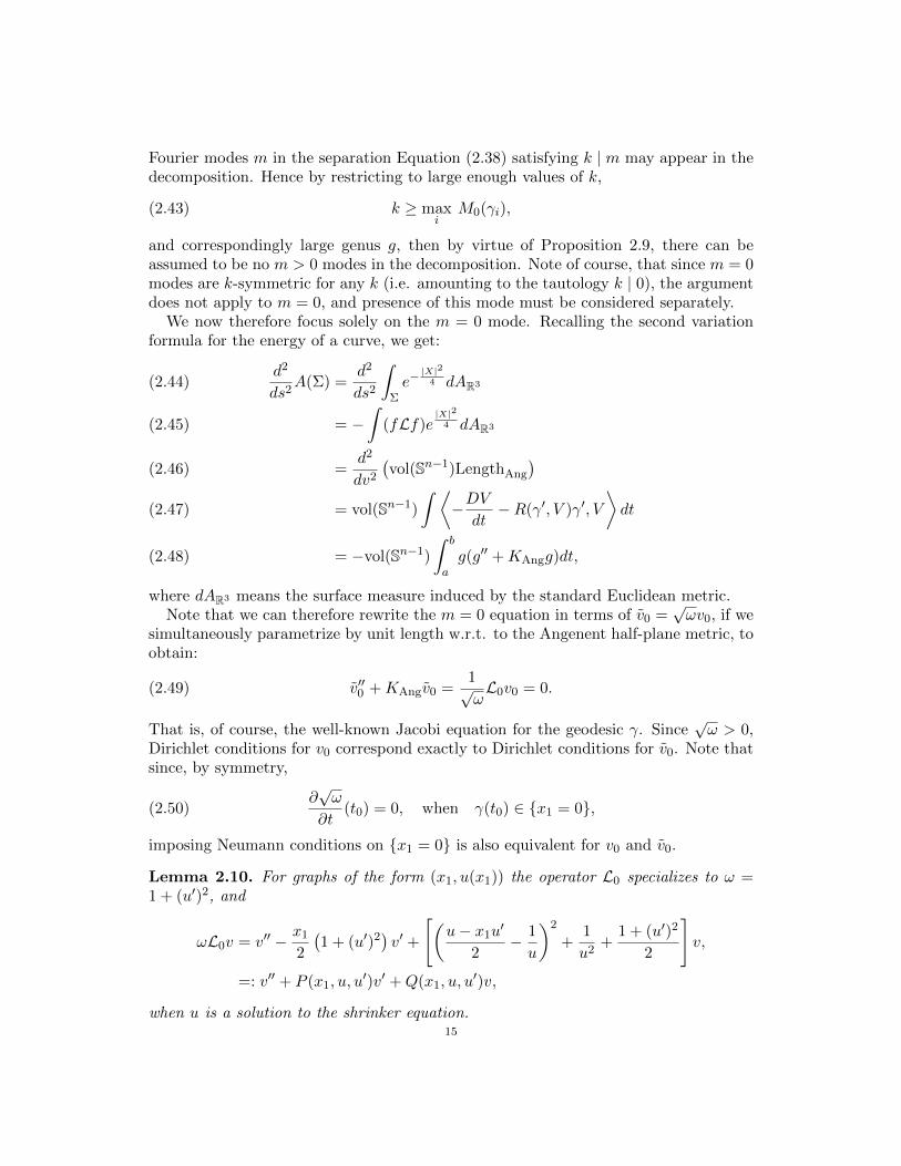
Figure 3. Jacobi field J on S3 ⊆ S2, with Neumann condition on{x = 0}. Drawn w.r.t. polar coordinates around (0, 1), where ϕ is theangle out from the x2-axis in Figure 2.1. Point of intersection with T2

indicated.

For solution graphs of the form (f(x2), x2) we have ω = 1 + (f ′)2 and the formulais:

ωL0g = g′′ +

[1

x2− x2

2

] (1 + (f ′)2

)g′ +

[(x2f

′ − f2

− f ′

x2

)2

+(f ′)2

x22

+1 + (f ′)2

2

]g

=: g′′ +R(x2, f, f′)g′ + S(x2, f, f

′)g.

Let us as a preliminary consideration note that the mean curvature H has rotationalsymmetry, and is an eigenfunction with eigenvalue 1 (see [CM2]):

(2.51) LH = H,

and Neumann conditions on {x1 = 0}. The profile of T2 is convex as shown in [KMø],and thus since the sign of the mean curvature changes only at points of tangential

16

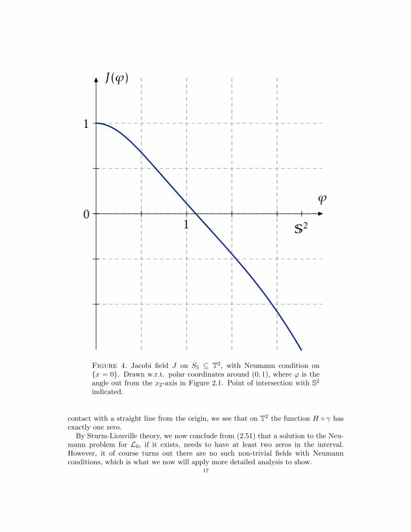
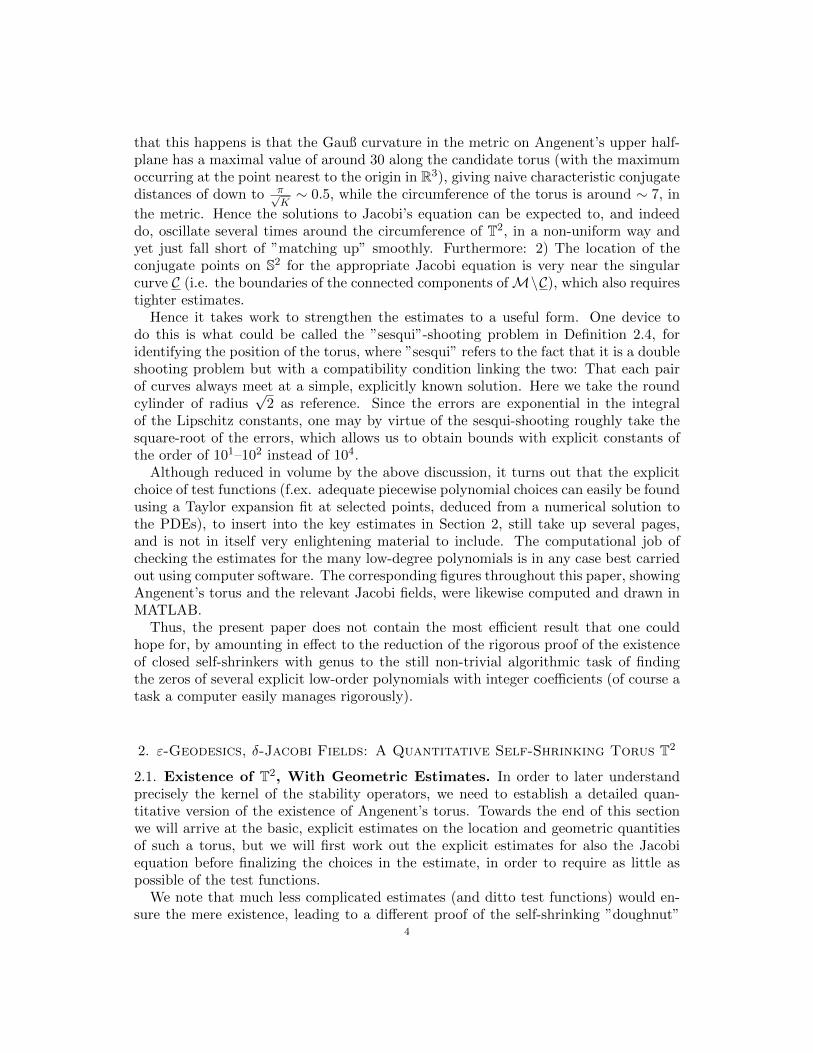
Figure 4. Jacobi field J on S5 ⊆ T2, with Neumann condition on{x = 0}. Drawn w.r.t. polar coordinates around (0, 1), where ϕ is theangle out from the x2-axis in Figure 2.1. Point of intersection with S2

indicated.

contact with a straight line from the origin, we see that on T2 the function H ◦ γ hasexactly one zero.

By Sturm-Liouville theory, we now conclude from (2.51) that a solution to the Neu-mann problem for L0, if it exists, needs to have at least two zeros in the interval.However, it of course turns out there are no such non-trivial fields with Neumannconditions, which is what we now will apply more detailed analysis to show.

17

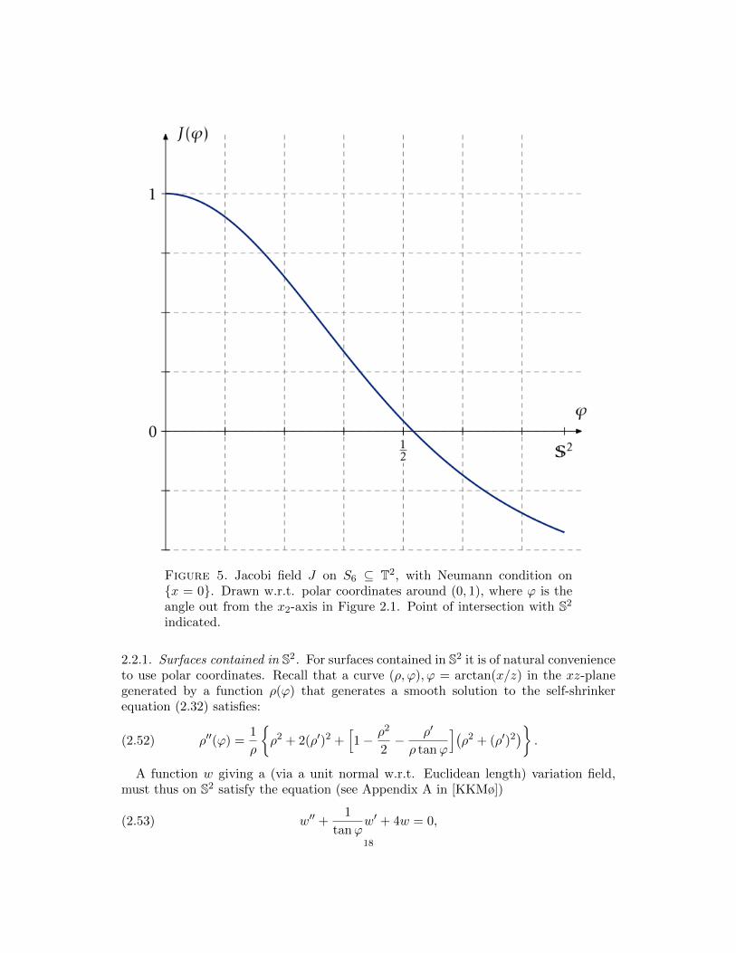
Figure 5. Jacobi field J on S6 ⊆ T2, with Neumann condition on{x = 0}. Drawn w.r.t. polar coordinates around (0, 1), where ϕ is theangle out from the x2-axis in Figure 2.1. Point of intersection with S2

indicated.

2.2.1. Surfaces contained in S2. For surfaces contained in S2 it is of natural convenienceto use polar coordinates. Recall that a curve (ρ, ϕ), ϕ = arctan(x/z) in the xz-planegenerated by a function ρ(ϕ) that generates a smooth solution to the self-shrinkerequation (2.32) satisfies:

(2.52) ρ′′(ϕ) =1

ρ

{ρ2 + 2(ρ′)2 +

[1− ρ2

2− ρ′

ρ tanϕ

](ρ2 + (ρ′)2

)}.

A function w giving a (via a unit normal w.r.t. Euclidean length) variation field,must thus on S2 satisfy the equation (see Appendix A in [KKMø])

(2.53) w′′ +1

tanϕw′ + 4w = 0,

18

with appropriate boundary conditions. The substitution x = cos(ϕ) in (2.53) givesLegendre’s differential equation, and the solution is:

w(ϕ) = C1Pl0(cosϕ) + C2Ql0(cosϕ),

where Pl and Ql are respectively the Legendre functions of the first and second kind,and l0 = (

√17− 1)/2 is the positive root of l(l + 1) = 4.

For the surface S1 ⊆ S2, which is generated by rotation of the radius 2 quarter-circle, the boundary conditions in the theorem are w′(0) = 0 and w′(π2 ) = 0. But sinceQl0(cosϕ) has a pole at ϕ = 0, we see that C2 = 0. Thus, if we normalize w so thatC1 = 1, we have by the first condition that w = Pl0(cosϕ). However,

(2.54)dPl0(cosϕ)

dϕ |ϕ=π2

=

√π

2

√17 + 1

Γ(

1−√

174

)Γ(

5+√

174

) 6= 0,

and hence there is no such Neumann mode. By the preceding, we therefore concludethat under N -fold symmetry, for a large enough N > 0,

(2.55) kerLS1 = {0}, on S1 = S2 ∩ {x1 ≥ 0} [Neumann conditions].

As for the surface S3 ⊆ S2, which we let for definiteness be the component such that(2, 0) ∈ S3, again C1 = 1 and C2 = 0. Now, since by (2.4),

(2.56) Pl0(cos(∠(~e1, p+))) ≥ Pl0(cos(11

10 + 120)) ≥ 1

200 > 0,

we conclude again

(2.57) kerLS3 = {0} [Dirichlet conditions].

For S4 ⊆ S2, the component with (0, 2) ∈ S4, we see that with w′(π2 ) = 0 and fixing

w(π2 ) = 1, (C1

C2

)=

(Pl0(cos(π2 )) Ql0(cos(π2 ))ddϕPl0(cos(π2 )) d

dϕPl0(cos(π2 ))

)−1(10

)such that with these constants

w(∠(~e1, p+)) ≥ w(11

10)− 100εgap >12 > 0.

Thus on the surface S4 with Neumann and Dirichlet conditions as in the statement ofthe theorem, we also conclude

(2.58) kerLS4 = {0} [Neumann on {x1 = 0}, Dirichlet on S4 ∩ T2].

2.2.2. Surfaces Contained in T2. In this section we will show that the Jacobi fieldswith Neumann conditions u′0(0) = 0 (and normalized to u0(0) = 1), propagated fromrespectively the top and the bottom of the torus T2 from Section 2 have the followingend-point values at the point where T2 intersects the round 2-sphere of radius 2:

(2.59)

(u0(ttop)u′0(ttop)

)=

−2250 ± 10εgap

−3750 ± 10εgap

19

and

(2.60)

(u0(tbot)u′0(tbot)

)=

−7750 ± 10εgap

−8450 ± 10εgap,

where the notation is meant to imply that each component is contained in the corre-sponding intervals arising from both choices of sign.

This means firstly that the Dirichlet problems on each part (w/ Neumann conditionson P) have trivial kernel, that is:

kerLS5 = {0} [Neumann on {x1 = 0}, Dirichlet on S5 ∩ S2],(2.61)

kerLS6 = {0} [Neumann on {x1 = 0}, Dirichlet on S6 ∩ S2].(2.62)

Secondly, note that non-triviality of the kernel of L on T2∩{x1 ≥ 0} with Neumannconditions has now been reduced to the conditions

αu0(ttop) = βu0(ttop),

αu′0(ttop) = −βu′0(tbot),

for a non-zero pair (α, β) or in other words, singularity of the matrix N :

(2.63) N :=

(u0(ttop) −u0(tbot)u′0(ttop) u′0(tbot)

).

But in fact from (2.59)–(2.60) we see

(2.64) detN ≥ 95 > 0,

so we finally conclude that also

kerLS2 = {0} [Neumann on {x1 = 0}.To show the required estimates of the Jacobi fields, we consider first an approximate

solution V to the linearized equation on the approximate curve Γ from the previoussection.

Top: x1-graph (Jacobi Equation)

Let us consider the first part of Γ, graphical over the x1-axis, on x1 ∈ [0, 35 ]. Here,

we have the expressions (recall Lemma 2.10 for the definition of P an Q).∣∣∂2P (x1, ξ, U′)∣∣ = 0,∣∣∂3P (x1, u, ξ

′)∣∣ = |x1ξ

′|,∣∣∂2Q(x1, ξ, U′)∣∣ = 2

∣∣∣∣(ξ − x1U′

2− 1

ξ

)(1

2+

1

ξ2

)− 1

ξ3

∣∣∣∣ ,∣∣∂3Q(x1, u, ξ′)∣∣ =

∣∣∣∣x1

(u− x1ξ

′

2− 1

u

)− ξ′

∣∣∣∣ .Assume for a small δT1 > 0 the uniform bounds:∣∣V ′′ + P (x1, U, U

′)V ′ +Q(x1, U, U′)V∣∣ ≤ δT1 ,(2.65) ∣∣∂3P (x1, u, ξ

′)∣∣ |v′|+ ∣∣∂3Q(x1, u, ξ

′)∣∣ |v| ≤ x1(2x2

1 + 3),(2.66) ∣∣∂2Q(x1, ξ, U′)∣∣ |v| ≤ 8

5 −32x

21.(2.67)

20

We let Φ(x1) := |V ′(x1)− v′(x1)| and estimate:

Φ′(x1) ≤∣∣|V ′ − v′|′∣∣ a.e

= |V ′′ − v′′|≤∣∣P (x1, U, U

′)V ′ − P (x1, u, u′)v′∣∣+∣∣Q(x1, U, U

′)V −Q(x1, u, u′)v∣∣+ δT1

≤∣∣P (x1, U, U

′)∣∣ |V ′ − v′|+ ∣∣P (x1, U, U

′)− P (x1, u, u′)∣∣ |v′|

+∣∣Q(x1, U, U

′)∣∣ |V − v|+ ∣∣Q(x1, U, U

′)−Q(x1, u, u′)∣∣ |v|+ δT1

≤∣∣P (x1, U, U

′)∣∣ |V ′ − v′|+ ∣∣Q(x1, U, U

′)∣∣ |V − v|

+(∣∣∂3P (x1, u, ξ

′)∣∣ |v′|+ ∣∣∂3Q(x1, u, ξ

′)∣∣ |v|) |U ′ − u′|

+(((((((((∣∣∂2P (x1, ξ, U

′)∣∣|v′|+ ∣∣∂2Q(x1, ξ, U

′)∣∣ |v|) |U − u|+ δT1

≤∣∣P (x1, U, U

′)∣∣Φ(x1) +

∣∣Q(x1, U, U′)∣∣ ∫ x1

0Φ(s)ds+

∣∣Q(x1, U, U′)∣∣ |V (0)− v(0)|

+ x1(2x21 + 3)|U ′(x1)− u′(x1)|+ (8

5 −32x

21)|U(x1)− u(x1)|+ δT1 .

We integrate on [0, x1] to get:

Φ(x1) ≤∫ x1

0

[∣∣P (s, U, U ′)∣∣+

∫ x1

0

∣∣Q(t, U, U ′)∣∣ dt]Φ(s)ds+

(∫ x1

0

∣∣Q(s, U, U ′)∣∣ ds) |V (0)− v(0)|

+

∫ x1

0s(2s2 + 3)|U ′(s)− u′(s)|ds+

∫ x1

0(8

5 −32s

2)|U(s)− u(s)|ds+ δT1 x1.

Recall the estimates for |U ′(s)− u′(s)|, which lead to:∫ x1

0s(2s2 + 3)|U ′(s)− u′(s)|ds ≤

[45 |U(0)− u(0)|+ εT1

] ∫ x1

0s2(2s2 + 3) exp

{5215s

2}ds

≤ 920 |U(0)− u(0)|+ 14

25εT1 .

Note also that from the estimates for |U − u| from |U ′ − u′|, we have already onceestimated the integral of the latter. We now need the sizes of these elementary Gaussiandouble integrals: ∫ 3

5

0(8

5 −32x

21)

(1 +

∫ x1

0

4s5 exp

{5215s

2}ds

)dx1 ≤

23

25,∫ 3

5

0(8

5 −32x

21)

∫ x1

0s exp

{5215s

2}dsdx1 ≤

7

100.

Thus ∫ 35

0(8

5 −32s

2)|U(s)− u(s)|ds ≤ 2325 |U(0)− u(0)|+ 7

100εT1 .

Now, we will furthermore assume the following bounds on the test functions, per-taining to the approximation by ε-geodesics:∫ x1

0|P (s, U, U ′)|ds ≤

∫ x1

0s(7

5s2 + 7

10)ds ≤ 720x

21(x2

1 + 1),(2.68) ∫ x1

0

∣∣Q(s, U, U ′)∣∣ ds ≤ ∫ x1

0(16

5 s2 + 5

2)ds ≤ 1615x

31 + 5

2x1.(2.69)

21

Applying Gronwall-Bellman again, to these new estimates, we see, using also thatV (0) = v(0) = 1 by assumption:

Φ(x1) ≤[∫ x1

0s(2s2 + 3)|U ′(s)− u′(s)|ds+

∫ x1

0(8

5 −32s

2)|U(s)− u(s)|ds+ δT1 x1

]×

exp

{∫ x1

0

∣∣P (s, U, U ′)∣∣ ds+ x1

∫ x1

0

∣∣Q(s, U, U ′)∣∣ ds}

≤[

137100 |U(0)− u(0)|+ 63

100εT1 + 3

5δT1

]×

exp{

720x

21(x2

1 + 1) + 1615x

41 + 5

2x21

}.

Thus

|V ′(35)− v′(3

5)| ≤ 235 |U(0)− u(0)|+ 11

5 εT1 + 51

25δT1 ,

|V (35)− v(3

5)| ≤ 1310 |U(0)− u(0)|+ 3

5εT1 + 11

50δT1 .

Here, the last estimate followed by integrating the estimates above, and using againthat V (0) = v(0).

Top: x2-graph to the sphere (Jacobi Equation)

We consider the next part of Γ, graphical over the x2-axis in the region [yS2 , uT (3/5)](in the backwards direction). Here, we have the expressions:

∣∣∂2R(x2, ξ, F′)∣∣ = 0,∣∣∂3R(x2, f, ξ

′)∣∣ = 2

∣∣∣∣ 1

x2− x2

2

∣∣∣∣ |ξ′|,∣∣∂2S(x2, ξ, F′)∣∣ =

∣∣∣∣( 1

x2− x2

2

)F ′ +

ξ

2

∣∣∣∣ ,∣∣∂3S(x2, f, ξ′)∣∣ =

∣∣∣∣( 1

x2− x2

2

)(x2ξ

′ − f) +4ξ′

x22

∣∣∣∣ .Assume for a small δT2 > 0 the uniform bounds:

∣∣G′′ +R(x2, F, F′)G′ + S(x2, F, F

′)G∣∣ ≤ δT2 ,(2.70) ∣∣∂3R(x2, u, ξ

′)∣∣ |g′|+ ∣∣∂3S(x2, f, ξ

′)∣∣ |g| ≤ 3

10 + 3320 (x2 − yS2)5(2.71) ∣∣∂2S(x2, ξ, U

′)∣∣ |g| ≤ η(x2),(2.72)

where

(2.73) η(x2) =

{41200− 3

10 (x2 − yS2)2 , x2 ∈ [yS2 ,52],

34− 5

2(x2 − yS2) + 21

10(x2 − yS2)2 , x2 ∈ [5

2, uT (3/5)].

22

We let Ψ(x2) := |G′(x2)− g′(x2)| and estimate:

Ψ′(x2) ≤∣∣|G′ − g′|′∣∣ a.e

= |G′′ − g′′|≤∣∣R(x2, F, F

′)G′ −R(x2, f, f′)g′∣∣+∣∣S(x2, F, F

′)G− S(x2, f, f′)g∣∣+ δT2

≤∣∣R(x2, F, F

′)∣∣ |G′ − g′|+ ∣∣R(x2, F, F

′)−R(x2, f, f′)∣∣ |g′|

+∣∣S(x2, F, F

′)∣∣ |G− g|+ ∣∣S(x2, F, F

′)− S(x2, f, f′)∣∣ |g|+ δT2

≤∣∣R(x2, F, F

′)∣∣ |G′ − g′|+ ∣∣S(x2, F, F

′)∣∣ |G− g|

+(∣∣∂3R(x2, f, ξ

′)∣∣ |g′|+ ∣∣∂3S(x2, f, ξ

′)∣∣ |g|) |F ′ − f ′|

+∣∣∂2S(x2, ξ, F

′)∣∣ |g||F − f |+ δT2

≤∣∣R(x2, F, F

′)∣∣Ψ(x2) +

∣∣S(x2, F, F′)∣∣ ∫ x2

uT (3/5)Ψ(s)ds+

∣∣S(x2, F, F′)∣∣ |G(uT (3/5))− g(uT (3/5))|

+[

310 + 33

20 (x2 − yS2)5]|F ′(x2)− f ′(x2)|+ η(x2)|F (x2)− f(x2)|+ δT2 .

We integrate on [x2, uT (3/5)] to get:

Ψ(x2) ≤∫ uT (3/5)

x2

[∣∣R(s, F, F ′)∣∣+

∫ uT (3/5)

x2

∣∣S(t, F, F ′)∣∣ dt]Ψ(s)ds

+

(∫ uT (3/5)

x2

∣∣S(s, F, F ′)∣∣ ds) |G(uT (3/5))− g(uT (3/5))|

+

∫ uT (3/5)

x2

[310 + 33

20 (s− yS2)5]|F ′(s)− f ′(s)|ds+

∫ uT (3/5)

x2

η(s)|F (s)− f(s)|ds

+ |G′(uT (3/5))− g′(uT (3/5))|+ δT2 (uT (3/5)− x2).

Recall, we have above shown the estimates:

|F ′(x2)− f ′(x2)| ≤[(13

8 −x22 )|F (uT (3/5))− f(uT (3/5))|+ |F ′(uT (3/5))− f ′(uT (3/5))|

+ εT2 (uT (3/5)− x2)]

exp{

74 −

910 (x2 − yS2)2 +

(138 −

x22

)(uT (3/5)− x2)

},

|F (uT (3/5))− f(uT (3/5))| ≤ 1012

(925ε

T1 + 23

80 |U(0)− u(0)|),

|F ′(uT (3/5))− f ′(uT (3/5))| ≤(

1012

)2(εT1 + 4

5 |U(0)− u(0)|).

We therefore get the bound:

∫ uT (3/5)

yS2

[310 + 33

20 (s− yS2)5]|F ′(s)− f ′(s)|ds ≤ 80

25 |U(0)− u(0)|+ 6εT1 + 2710ε

T2 .

23

Again, we will need the sizes of some elementary Gaussian double integrals:

∫ uT (3/5)

yS2

η(x2)

(1 +

∫ uT (3/5)

x2

(138 −

s2) exp

{74 −

910 (s− yS2)2 +

(138 −

s2

)(uT (3/5)− s)

}ds

)dx2 ≤ 29

50∫ uT (3/5)

yS2

∫ uT (3/5)

x2

η(x2) exp{

74 −

910 (s− yS2)2 +

(138 −

s2

)(uT (3/5)− s)

}dsdx2 ≤ 29

50 ,∫ uT (3/5)

yS2

∫ uT (3/5)

x2

η(x2)(uT (3/5)− s) exp{

74 −

910 (s− yS2)2 +

(138 −

s2

)(uT (3/5)− s)

}dsdx2 ≤ 19

50 .

Thus ∫ uT (3/5)

yS2

η(x2)|F (x2)− f(x2)|dx2 ≤ 12 |U(0)− u(0)|+ 29

50εT1 + 19

50εT2 .

Assume once again bounds for the ε-geodesics:∫ uT (3/5)

x2

|R(s, F, F ′)|ds ≤ −1625x

22 + 22

10x2 − 1825 ,(2.74) ∫ uT (3/5)

x2

∣∣S(s, F, F ′)∣∣ ds ≤ − 27

100x22 + 7

25x2 + 1910 .(2.75)

By Gronwall-Bellman with the new estimates, we see:

Ψ(x2) ≤

[(∫ uT (3/5)

x2

∣∣S(s, F, F ′)∣∣ ds) |G(uT (3/5))− g(uT (3/5))|

+

∫ uT (3/5)

x2

[310 + 33

20 (x2 − yS2)5]|F ′(s)− f ′(s)|ds

+

∫ uT (3/5)

x2

η(x2)|F (s)− f(s)|ds+ δT2 (uT (3/5)− x2) + |G′(uT (3/5))− g′(uT (3/5))|

]×

exp

{∫ uT (3/5)

x2

∣∣R(s, F, F ′)∣∣ ds+ (uT (3/5)− x2)

∫ uT (3/5)

x2

∣∣S(s, F, F ′)∣∣ ds}

≤24[

3120

(1310 |U(0)− u(0)|+ 3

5εT1 + 11

50δT1

)+ 80

25 |U(0)− u(0)|+ 6εT1 + 2710ε

T2

+ 12 |U(0)− u(0)|+ 29

50εT1 + 19

50εT2 + (49

16 −4123)δT2 +

235 |U(0)− u(0)|+ 11

5 εT1 + 51

25δT1

|u′(35)|

].

As before, we thus have the estimate:

|Ψ(yS2)| = |G′(yS2)− g′(yS2)| ≤ 237|U(0)− u(0)|+ 228εT1 + 74εT2 + 53δT1 + 31δT2 ,

24

where we used 1/|u′(35)| ≤ 9

10 . By integration, we can again accurately estimate the‖·‖C0-norm, although here it suffices to use a simple supremum bound on the integrand:

|G(yS2)− g(yS2)| ≤ |G(uT (3/5))− g(uT (3/5))|+ |yS2 − uT (3/5)||Ψ(yS2)|= 13

10 |U(0)− u(0)|+ 35εT1 + 11

50δT1 + 13

10

(237|U(0)− u(0)|+ 228εT1 + 74εT2 + 53δT1 + 31δT2

)≤ 310|U(0)− u(0)|+ 297εT1 + 97εT2 + 70δT1 + 41δT2 .

Bottom: x1-graph (Jacobi Equation)Let us consider the first part of Γ, graphical over the x1-axis. Here, we have the

expressions: ∣∣∂2P (x1, ξ, U′)∣∣ = 0,∣∣∂3P (x1, u, ξ

′)∣∣ = |x1ξ

′|,∣∣∂2Q(x1, ξ, U′)∣∣ = 2

∣∣∣∣(ξ − x1U′

2− 1

ξ

)(1

2+

1

ξ2

)− 1

ξ3

∣∣∣∣ ,∣∣∂3Q(x1, u, ξ′)∣∣ =

∣∣∣∣x1

(u− x1ξ

′

2− 1

u

)− ξ′

∣∣∣∣ .Assume for a small δB1 > 0 the uniform bounds:∣∣V ′′ + P (x1, U, U

′)V ′ +Q(x1, U, U′)V∣∣ ≤ δB1 ,(2.76) ∣∣∂3P (x1, u, ξ

′)∣∣ |v′|+ ∣∣∂3Q(x1, u, ξ

′)∣∣ |v| ≤ 2,(2.77) ∣∣∂2Q(x1, ξ, U

′)∣∣ |v| ≤ 41− 80x1.(2.78)

We let Φ(x1) := |V ′(x1)− v′(x1)| and estimate:

Φ′(x1) ≤∣∣|V ′ − v′|′∣∣ a.e

= |V ′′ − v′′|≤∣∣P (x1, U, U

′)V ′ − P (x1, u, u′)v′∣∣+∣∣Q(x1, U, U

′)V −Q(x1, u, u′)v∣∣+ δB1

≤∣∣P (x1, U, U

′)∣∣ |V ′ − v′|+ ∣∣P (x1, U, U

′)− P (x1, u, u′)∣∣ |v′|

+∣∣Q(x1, U, U

′)∣∣ |V − v|+ ∣∣Q(x1, U, U

′)−Q(x1, u, u′)∣∣ |v|+ δB1

≤∣∣P (x1, U, U

′)∣∣ |V ′ − v′|+ ∣∣Q(x1, U, U

′)∣∣ |V − v|

+(∣∣∂3P (x1, u, ξ

′)∣∣ |v′|+ ∣∣∂3Q(x1, u, ξ

′)∣∣ |v|) |U ′ − u′|

+∣∣∂2Q(x1, ξ, U

′)∣∣ |v||U − u|+ δB1

Hence:

≤∣∣P (x1, U, U

′)∣∣Φ(x1) +

∣∣Q(x1, U, U′)∣∣ ∫ x1

0Φ(s)ds+

∣∣Q(x1, U, U′)∣∣ |V (0)− v(0)|

+ 2|U ′(x1)− u′(x1)|+ (41− 80x1)|U(x1)− u(x1)|+ δB1 .

25

We integrate on [0, x1] to get:

Φ(x1) ≤∫ x1

0

[∣∣P (s, U, U ′)∣∣+

∫ x1

0

∣∣Q(t, U, U ′)∣∣ dt]Φ(s)ds+

(∫ x1

0

∣∣Q(s, U, U ′)∣∣ ds) |V (0)− v(0)|

+ 2

∫ x1

0|U ′(s)− u′(s)|ds+

∫ x1

0(41− 80s)|U(s)− u(s)|ds+ δB1 x1.

Recall the estimates:

2

∫ x1

0|U ′(s)− u′(s)|ds ≤ 2|U(0)− u(0)|

∫ x1

0(29

5 s+ 120) exp

{495 s

2 + s4

}ds

+ 2εB1

∫ x1

0s exp

{495 s

2 + s4

}ds

≤ 365 |U(0)− u(0)|+ 6

5εB1 .

Note also that from the estimates for |U − u| from |U ′ − u′|, we have already onceestimated the integral of the latter. We now need the sizes of these elementary Gaussiandouble integrals:∫ 1

2

0(41− 80x1)

(1 +

∫ x1

0(29

5 s+ 120) exp

{495 s

2 + s4

}ds

)dx1 ≤

67

5,∫ 1

2

0

∫ x1

0(41− 80x1)s exp

{495 s

2 + s4

}dsdx1 ≤

12

25.

Thus ∫ 12

0(41− 80x1)|U(x1)− u(x1)|dx1 ≤ 67

5 |U(0)− u(0)|+ 12

25εB1 .

Now, we will furthermore assume the bounds pertaining to the ε-geodesics:∫ x1

0|P (s, U, U ′)|ds ≤ 4

9x2

1,(2.79) ∫ x1

0

∣∣Q(s, U, U ′)∣∣ ds ≤ 4− 16(x1 − 1

2)2.(2.80)

Again, by Gronwall-Bellman we see (with V (0) = v(0)):

Φ(x1) ≤[2

∫ x1

0|U ′(s)− u′(s)|ds+

∫ x1

0(41− 80s)|U(s)− u(s)|ds+ δB1 x1

]×

exp

{∫ x1

0

∣∣P (s, U, U ′)∣∣ ds+ x1

∫ x1

0

∣∣Q(s, U, U ′)∣∣ ds}

≤[

1035 |U(0)− u(0)|+ 42

25εB1 + δB1 x1

]×

exp{

49x

21 + 4x1 − 16x1(x1 − 1

2)2}.

Thus

|V ′(12)− v′(1

2)| ≤ 171|U(0)− u(0)|+ 14εB1 + 389 δ

B1 ,

|V (12)− v(1

2)| ≤ 31|U(0)− u(0)|+ 5120ε

B1 + 11

5 δB1 .

Here, the last estimate followed by integration and using again V (0) = v(0).26

Bottom: x2-graph to cylinder (Jacobi Equation)

We consider the next part of Γ, graphical over the x2-axis over [a0,√

2]. Here, wehave the expressions:∣∣∂2R(x2, ξ, F

′)∣∣ = 0,∣∣∂3R(x2, f, ξ

′)∣∣ = 2

∣∣∣∣ 1

x2− x2

2

∣∣∣∣ |ξ′|,∣∣∂2S(x2, ξ, F′)∣∣ =

∣∣∣∣( 1

x2− x2

2

)F ′ +

ξ

2

∣∣∣∣ ,∣∣∂3S(x2, f, ξ′)∣∣ =

∣∣∣∣( 1

x2− x2

2

)(x2ξ

′ − f) +4ξ′

x22

∣∣∣∣ .Assume for a small δB2 > 0 the uniform bounds:∣∣G′′ +R(x2, F, F

′)G′ + S(x2, F, F′)G∣∣ ≤ δB2 ,(2.81) ∣∣∂3R(x2, u, ξ

′)∣∣ |g′|+ ∣∣∂3S(x2, f, ξ

′)∣∣ |g| ≤ 4

5+ 8

(x2 −

√2)2,(2.82) ∣∣∂2S(x2, ξ, U

′)∣∣ |g| ≤ 24

50− 3

4

(x2 −

√2)2.(2.83)

We let Ψ(x2) := |G′(x2)− g′(x2)| and estimate:

Ψ′(x2) ≤∣∣|G′ − g′|′∣∣ a.e

= |G′′ − g′′|≤∣∣R(x2, F, F

′)G′ −R(x2, f, f′)g′∣∣+∣∣S(x2, F, F

′)G− S(x2, f, f′)g∣∣+ δB2

≤∣∣R(x2, F, F

′)∣∣ |G′ − g′|+ ∣∣R(x2, F, F

′)−R(x2, f, f′)∣∣ |g′|

+∣∣S(x2, F, F

′)∣∣ |G− g|+ ∣∣S(x2, F, F

′)− S(x2, f, f′)∣∣ |g|+ δB2

≤∣∣R(x2, F, F

′)∣∣ |G′ − g′|+ ∣∣S(x2, F, F

′)∣∣ |G− g|

+(∣∣∂3R(x2, f, ξ

′)∣∣ |g′|+ ∣∣∂3S(x2, f, ξ

′)∣∣ |g|) |F ′ − f ′|

+∣∣∂2S(x2, ξ, F

′)∣∣ |g||F − f |+ δB2

≤∣∣R(x2, F, F

′)∣∣Ψ(x2) +

∣∣S(x2, F, F′)∣∣ ∫ x2

0Ψ(s)ds+

∣∣S(x2, F, F′)∣∣ |G(a0)− g(a0)|

+

[4

5+ 8

(x2 −

√2)2]|F ′(x2)− f ′(x2)|+

[24

50− 3

4

(x2 −

√2)2]|F (x2)− f(x2)|+ δB2 .

We integrate on [a0, x2] to get:

Ψ(x2) ≤∫ x2

a0

[∣∣R(s, F, F ′)∣∣+

∫ x2

a0

∣∣S(t, F, F ′)∣∣ dt]Ψ(s)ds+

(∫ x2

a0

∣∣S(s, F, F ′)∣∣ ds) |G(a0)− g(a0)|

+

∫ x2

a0

[45 + 8(s−

√2)2]|F ′(s)− f ′(s)|ds+

∫ x2

a0

[2450 −

34(s−

√2)2]|F (s)− f(s)|ds

+ |G′(a0)− g′(a0)|+ δB2 (x2 − a0).27

Recall, we have above shown the estimates:

|F ′(x2)− f ′(x2)| ≤[(16

25x2 − 37)|F (a0)− f(a0)|+ |F ′(a0)− f ′(a0)|+ εB2 (x2 − a0)

]× exp

{910 −

1110

(x2 − 3

2

)2+ (x2 − a0)

(1625x2 − 3

7

)},

|F (a0)− f(a0)| ≤ 1012

(35εB1 + 23

5 |U(0)− u(0)|)

|F ′(a0)− f ′(a0)| ≤(

1012

)2(28

5 εB1 + 39|U(0)− u(0)|).

We therefore get the bound:

∫ √2

a0

[45 + 8(s−

√2)2]|F ′(s)− f ′(s)|ds ≤ 78|U(0)− u(0)|+ 12εB1 + 9

10εB2 .

Again, we will need the sizes of some elementary Gaussian double integrals:

∫ √2

a0

[2450 −

34(x2 −

√2)2](

1 +

∫ x2

a0

(1625s−

37) exp

{910 −

1110

(s− 3

2

)2+ (s− a0)

(1625s−

37

)}ds

)dx2

≤ 3

10,∫ √2

a0

∫ x2

a0

[2450 −

34(x2 −

√2)2]

exp{

910 −

1110

(x2 − 3

2

)2+ (x2 − a0)

(1625x2 − 3

7

)}dsdx2 ≤ 1

5 ,∫ √2

a0

∫ x2

a0

[2450 −

34(x2 −

√2)2]

(s− a0) exp{

910 −

1110

(x2 − 3

2

)2+ (x2 − a0)

(1625x2 − 3

7

)}dsdx2 ≤

7

125.

Thus

∫ √2

a0

[2450 −

34(x2 −

√2)2]|F (x2)− f(x2)|dx2 ≤ 197

30 |U(0)− u(0)|+ 4750ε

B1 + 7

125εB2 .

Assume again bounds for the ε-geodesics:

∫ x2

a0

|R(s, F, F ′)|ds ≤ 920 −

34(x2 −

√2)2,(2.84) ∫ x2

a0

∣∣S(s, F, F ′)∣∣ ds ≤ x2 − 2

5 .(2.85)

28

By Gronwall-Bellman with the new estimates, we see:

Ψ(x2) ≤

[(∫ x2

a0

∣∣S(s, F, F ′)∣∣ ds) |G(a0)− g(a0)|+

∫ x2

a0

[45 + 8(s−

√2)2]|F ′(s)− f ′(s)|ds

+

∫ x2

a0

[2450 −

34(x2 −

√2)2]|F (s)− f(s)|ds+ δB2 (x2 − a0) + |G′(a0)− g′(a0)|

]×

exp

{∫ x2

a0

∣∣R(s, F, F ′)∣∣ ds+ (x2 − a0)

∫ x2

a0

∣∣S(s, F, F ′)∣∣ ds}

≤6320

[31|U(0)− U(0)|+ 51

20εB1 + 11

5 δB1 + 78|U(0)− u(0)|+ 12εB1 + 9

10εB2 + 197

30 |U(0)− u(0)|

+ 4750ε

B1 + 7

125εB2 + (

√2− a0)δB2 +

171|U(0)− u(0)|+ 14εB1 + 389 δ

B1

|u′(12)|

]

Thus

|G′(12)− g′(1

2)| ≤ 813|U(0)− u(0)|+ 86εB1 + 3εB2 + 9527δ

B1 + (

√2− a0)δB2 ,

|G(12)− g(1

2)| ≤ 522|U(0)− u(0)|+ 56εB1 + 2εB2 + 11δB1 + 910δ

B2 .

We see that, with matched initial conditions, choosing all approximation constants

εT/Bi and δ

T/Bi at the order of 10−1–10−3 (depending on each particular coefficient)

suffices to conclude the estimates in (2.59)–(2.60), and hence one may, with such testfunctions, rigorously verify that locations of the Jacobi functions are indeed accuratelyshown in Figures 3–6, such that the conclusions in Theorem 2.7 hold true. Hence themain claim, the existence and properties of the closed self-shrinkers in Theorem 1 isalso verified.

References

[AI] S. Angenent, T. Ilmanen, D. Chopp, A computed example of nonuniqueness of mean curvatureflow in R3, Comm. Partial Differential Equations 20 (1995), no. 11–12, 1937–1958.

[AL86] U. Abresch, J. Langer, The normalized curve shortening flow and homothetic solutions, J. Diff.Geom. 23 (1986), 175–196.

[Anc06] H. Anciaux, Construction of Lagrangian self-similar solutions to the mean curvature flow inCn, Geom. Dedicata 120 (2006), 37-48.

[An92] S. Angenent, Shrinking doughnuts, Nonlinear diffusion equations and their equilibrium states,3 (Gregynog, 1989), 21–38, Progr. Nonlinear Diff. Equ. Appl. 7 (1992), Birkhauser, Boston.

[Ch94] D. Chopp, Computation of self-similar surfaces, Experiment. Math., 3 (1994).[CS] D. Chopp, J. Sethian, Flow under curvature: singularity formation, minimal surfaces, and

geodesics, Experiment. Math. 2 (1993), 235–255.[CM1] T. H. Colding, W. P. Minicozzi II, Shapes of embedded minimal surfaces, Proc. Natl. Acad. Sci.

USA 103 (2006), no. 30, 11106–11111.[CM2] T. H. Colding, W. P. Minicozzi II, The space of embedded minimal surfaces in a 3-manifold. I.

Estimates off the axis for disks, Ann. of. Math (2) 160 (2004), no. 1, 27-68.[CM3] T. H. Colding, W. P. Minicozzi II, The space of embedded minimal surfaces in a 3-manifold. II.

Multi-valued graphs in disks, Ann. of. Math (2) 160 (2004), no. 1, 69-92.[CM4] T. H. Colding, W. P. Minicozzi II, The space of embedded minimal surfaces in a 3-manifold.

III. Planar domains, Ann. of. Math (2) 160 (2004), no. 2, 523-572.

29

[CM5] T. H. Colding, W. P. Minicozzi II, The space of embedded minimal surfaces in a 3-manifold.IV. Locally simply connected, Ann. of. Math (2) 160 (2004), no. 2, 573-615.

[CM6] T. H. Colding, W. P. Minicozzi II, The space of embedded minimal surfaces in a 3-manifold. V.Fixed genus, preprint.

[CM7] T.H. Colding, W.P. Minicozzi II, Smooth compactness of self-shrinkers, arXiv:0907.2594.[CM8] T.H. Colding, W. P. Minicozzi II, Generic mean curvature flow I; generic singularities, preprint,

http://arxiv.org/pdf/0908.3788.[CM9] T.H. Colding, W.P. Minicozzi II, Generic mean curvature flow II; dynamics of a closed smooth

singularity, in preparation.[Ec] Klaus Ecker, Regularity theory for mean curvature flow, Birkhauser 2004.[Hu90] G. Huisken, Asymptotic behavior for singularities of the mean curvature flow, J. Differential

Geom. 31 (1990), no. 1, 285–299.[Hu93] G. Huisken, Local and global behaviour of hypersurfaces moving by mean curvature. Differential

geometry: partial differential equations on manifolds (Los Angeles, CA, 1990),175–191, Proc.Sympos. Pure Math., 54, Part 1, Amer. Math. Soc., Providence, RI, 1993.

[Ka97] N. Kapouleas, Complete embedded minimal surfaces of finite total curvature, J. DifferentialGeom. 47 (1997), no. 1, 95–169.

[Ka95] N. Kapouleas, Constant mean curvature surfaces by fusing Wente tori, Invent. Math, 119(1995), 443-518.

[Ka05] N. Kapouleas, Constructions of minimal surfaces by gluing minimal immersions, Global theoryof minimal surfaces, 489–524, Clay Math. Proc., 2, Amer. Math. Soc., Providence, RI, 2005.

[Ka11] N. Kapouleas, Doubling and Desingularization Constructions for Minimal Surfaces, Volume inhonor of Professor Richard M. Schoen’s 60th birthday, arXiv:1012.5788v1.

[Ka] N. Kapouleas, A desingularization theorem for minimal surfaces in the compact case withoutsymmetries, in preparation.

[KKMø] N. Kapouleas, S. J. Kleene, N. M. Møller, Mean curvature self-shrinkers of high genus: Non-compact examples, preprint 2010, arXiv:1106.5454.

[KMø] S. Kleene, N.M. Møller, Self-shrinkers with a rotational symmetry, to appear in Trans. Amer.Math. Soc. (2011).

[Mø] N. M. Møller, Mean Curvature Self-shrinkers with Genus and Asymptotically Conical Ends, PhDdissertation, MIT, April 2012.

[Ng06] X.H. Nguyen, Construction of complete embedded self-similar surfaces under flow curvatureflow. Part I., arXiv:math/0610695; Trans. of the Amer. Math. Soc. 361 (2009), 1683–1701.

[Ng07] X.H. Nguyen, Construction of complete embedded self-similar surfaces under flow curvatureflow. Part II., arXiv:0704.0981; Adv. Differential Equations 15 (2010), 503–530.

[Ng11] X.H. Nguyen, Construction of complete embedded self-similar surfaces under mean curvatureflow. Part III., arXiv:1106.5272.

[Tr96] M. Traizet, Construction de surfaces minimales en recollant des surfaces de Scherk, Ann. Inst.Fourier (Grenoble), 46 (1996), pp. 1385-1442.

Niels Martin Møller, Fine Hall, Princeton University, NJ 08540.E-mail address: moller@math.princeton.edu

30