
Seepage and Slope Stability of Chinese Hydropower … 9 Seepage and Slope Stability of Chinese...
18
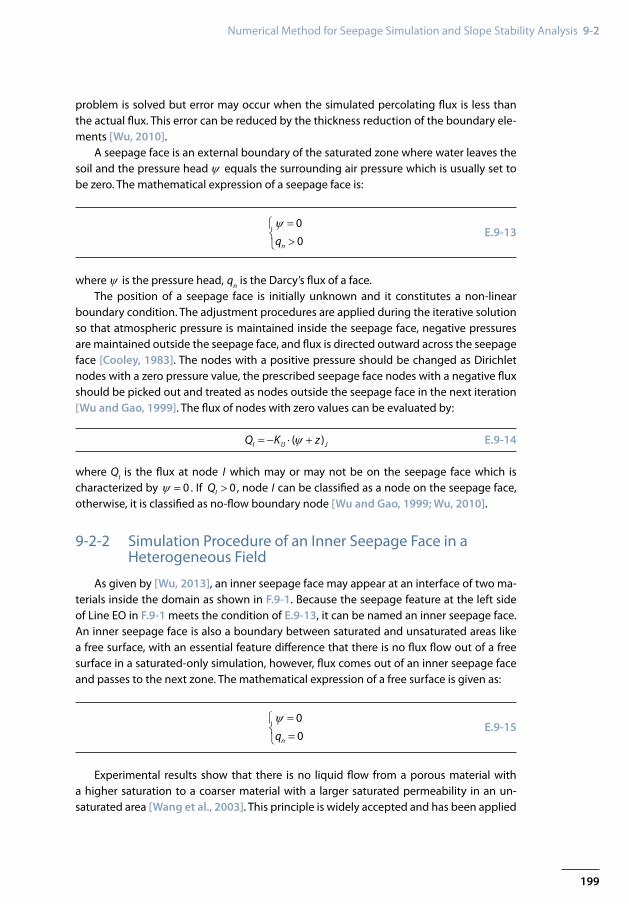
τ σ n P 1 (entrance point) P 2 (exit point) Author: Mengxi Wu 9 Seepage and Slope Stability of Chinese Hydropower Dams Motivation Hydropower dams are growing bigger and are placed in regions with high natural disaster probabilities. Knowledge on seepage and slope stability of these structures is de- sirable. Main Results A software tool to compute seepage stimulations and slope stability analysis has been created and applied to a number of examples of Chinese hydropower dams.
Transcript of Seepage and Slope Stability of Chinese Hydropower … 9 Seepage and Slope Stability of Chinese...
195
Chapter 9-x
τσn
P1 (entrance point)
P2 (exit point)
Author:Mengxi Wu
9Seepage and Slope Stability of Chinese Hydropower Dams
MotivationHydropower dams are growing bigger and are placed in regions with high natural
disaster probabilities. Knowledge on seepage and slope stability of these structures is de-sirable.
Main ResultsA software tool to compute seepage stimulations and slope stability analysis has been
created and applied to a number of examples of Chinese hydropower dams.
196
9 Seepage and Slope Stability of Chinese Hydropower Dams
9-1 Problem StatementSeepage simulation and slope stability analysis are steps necessary in the risk analysis
procedures of embankment dams, nature and engineering slopes. As part of the work in WP4, our research is mainly focused on improving the numerical methodology of seepage and slope stability analysis.
Catastrophic failures of embankment dams can occur as a result of subsurface erosion. They are likely to occur without any apparent warning, at full reservoir, sometimes many years after the reservoir has been put into operation. The erosion may start at springs feed by seepage and proceed insidiously upstream toward the reservoir, following lines of least resistance along foundation slabs, conduits, or irregularities in the bedrock, or it may develop entirely in the subsoil in a pattern that depends on unknown details of the strati-fication. When the erosion channel reaches the reservoir it enlarges rapidly; the release of water may destroy the dam and its foundation and devastate the valley downstream. Failure of a dam by subsurface erosion thus ranks among the most serious accidents in civil engineering.
Internal erosion within the body of zoned embankment dams may also have serious consequences. The water retaining element or core of such dams, usually consisting of clay or other relatively impervious soils, may develop cracks as a result of differential set-tlements or other causes, may not be sealed tightly against the foundation or abutments, or under the influence of seepage pressures may tend to migrate, particle by particle, into the coarser shell materials intended to support the core. The loss of core material by migration or erosion may result in sinkholes, in weakening and dislocation of the fill mate-rial, and sometimes in a breakthrough to the reservoir. If this occurs, the results can be as catastrophic as those of subsurface erosion.
The occurrence of sliding failures in embankments and excavated slopes is common. Collapses in these cases often bring serious consequences to both life and property. The risks involved justify the need to adequately assess and assure safety. The choice of suit-able methods of safety analysis is important. Limit equilibrium methods provide a power-ful means of evaluating safety. The calculation of stresses of the conventional limit equi-librium methods is based on slices. The assumptions about the distribution of stresses between slices have to be made in those methods. The impact of seepage on the effective stresses of a slope with complicated underground flow situations can hardly be evaluated reliably by these methods. It is obvious that stresses from methods of slices may not agree with actual soil stresses in an unacceptably large extent in many situations, such as rock fill dams, and their foundations, river and water reservoir banks, and many nature and engineering slopes in rainy seasons. Meaningful stability analysis can be made only if the stress distribution within the structure can be predicted reliably [Clough and Woodward, 1967].
In this report, a finite element algorithm for variably saturated flow and a modified gradient procedure for slope stability based on a finite element stress analysis are pre-sented.
197
Numerical Method for Seepage Simulation and Slope Stability Analysis 9-2
9-2 Numerical Method for Seepage Simulation and Slope Stability Analysis
9-2-1 A Finite-Element Algorithm for Modelling Variably Saturated Flows
The standard approach to model variably saturated flow is through the use of numeri-cal solution to Richards’ equation (RE). This report provides a general, mass-conservative and computationally efficient multi-dimensional finite element algorithm for modeling variably saturated seepage [Wu, 2010; Wu et al., 2013]. Water flowing through porous media is described by the Darcy equation written in the form:
, r , r( ) ( ) ( )i j ij j ijq h k s K z k s Kψ= − = − + E.9-1
According to the mass conservative principle and E.9-1, Richards’ equation (1931) governing saturated-unsaturated flows in porous media can be deduced as:
, r ,
( )[ ( )] ( ) ]j ij i
sz k K Q
tψψ ψ ε ∂− + + =∂
E.9-2
In E.9-1 and E.9-2, q is the Darcy flux vector, r ( )k s or r ( )k ψ is the relative conductiv-ity, K is the tensor of permeability for saturated media, h is the hydraulic head, ψ is the pressure head, z is the elevation above a reference datum, ε is the porosity and Q is the source/sink term. The subscripts i, j = 1, …, D are spatial indices of the Cartesian coordi-nates, and D denotes the number of spatial dimension (2 or 3). Note that the summation convention is used for repeated indices. Van Genuchten’s (VG) equation [Van Genuchten, 1980] for the soil water retention curve and Mualem’s [Mualem, 1976] unsaturated rela-tive permeability function are used to describe the soil properties. The relationship be-tween saturation and pressure head is given by:
(1 | | ) , 0( )
( )1 1, 0
n mr
er
s ss
sαψ ψψψ
ψ
− + <− = = − ≥
E.9-3
Where se is the effective saturation, s is the saturation, sr is the residual saturation, α is a parameter related to the mean pore size, n a parameter related to the uniformity of the size distribution and 1 1/m n= − . Based on Mualem’s [Mualem, 1976] model, the relation-ship between effective saturation and relative permeability is given by :
1/2 1/ 2r ( ) [1 (1 ) ]m m
e e ek s s s= − − E.9-4
The finite element algorithm for E.9-2 given by [Wu, 2010] is:
1[ ( ) ( )] ( ) ( ) ( )n nIJ IJ J I IJ J IJ JK O F O K zψ ψ ψ ψ ψ ψ ψ−+ ⋅ = + ⋅ − ⋅ E.9-5
198
9 Seepage and Slope Stability of Chinese Hydropower Dams
Where:
, 1IJ , ,( ) ( )
e
n mI i r ij J j
e
K N k K N dψ ψ −
Ω= Ω∑∫ E.9-6
, 1
, 1IJ
1 ( )( ) ( )
e
n mn m
IJe
CO d
l tψψ β ψ δ
−−
Ω= Ω
∆∑∫ E.9-7
, 1
1IJ
1 ( )( ) ( )
e
n mn
IJe
CO d
l tψψ β ψ δ
−−
Ω= Ω
∆∑∫ E.9-8
I( )e
n I ILe
F q N dL QN dψΩ
= − + Ω∑∫ ∫
E.9-9
In E.9-7 and E.9-8:
1, 0
( )0, 0
ψβ ψ
ψ≥
= < E.9-10
11 1
, 1 1 1
1 1
( ) ( ), ( ) ( ) 0.01
( ) ( )( )
( ) ( 0.01), ( ) ( ) 0.01
0.01
n nn n n n
n n m n n
n
n nn n n n
C
θ ψ θ ψ β ψ ψ β ψ ψβ ψ ψ β ψ ψ
ψθ ψ θ ψ β ψ ψ β ψ ψ
−− −
− − −
− −
−⋅ − ⋅ ≥ ⋅ − ⋅=
− −⋅ − ⋅ <
E.9-11
In these finite element equations, l is the node number of an element, ijδ is the Kro-necker delta. N is the nodal basis shape function of an element and I or J is the serial num-ber of a node in the element, n is the iterative step of the time t, m is the iterative step for solving the seepage field at the time t n.
Dirichlet, Neumann, and seepage-face boundaries are considered. Dirichlet nodes, where the pressure heads are known, are described by:
I Iψ ψ= † E.9-12
where Iψ† are the known pressure heads at the node I. The I-th equation in E.9-5 is substi-tuted by E.9-12 directly.
Neumann boundaries which are also named as flux boundaries, are treated in E.9-5. If the soil of the elements related to a flux boundary is unsaturated and extremely dry, and the flux is relatively larger than the moisture conductivity, convergence difficulties may arise. Under these situations, the conductivity of the elements related to the boundary nodes is small and unable to transmit the water away quickly from the boundary node, resulting in a very large hydraulic gradient and unphysical surface pressure head bounds. The way to alleviate this problem is to provide a proper feedback in the matrix to the flux to keep the result within the physical bounds [Zhang et al., 2002]. The convergence
199
Numerical Method for Seepage Simulation and Slope Stability Analysis 9-2
problem is solved but error may occur when the simulated percolating flux is less than the actual flux. This error can be reduced by the thickness reduction of the boundary ele-ments [Wu, 2010].
A seepage face is an external boundary of the saturated zone where water leaves the soil and the pressure head ψ equals the surrounding air pressure which is usually set to be zero. The mathematical expression of a seepage face is:
00nq
ψ = >
E.9-13
where ψ is the pressure head, qn is the Darcy’s flux of a face.The position of a seepage face is initially unknown and it constitutes a non-linear
boundary condition. The adjustment procedures are applied during the iterative solution so that atmospheric pressure is maintained inside the seepage face, negative pressures are maintained outside the seepage face, and flux is directed outward across the seepage face [Cooley, 1983]. The nodes with a positive pressure should be changed as Dirichlet nodes with a zero pressure value, the prescribed seepage face nodes with a negative flux should be picked out and treated as nodes outside the seepage face in the next iteration [Wu and Gao, 1999]. The flux of nodes with zero values can be evaluated by:
( )I IJ JQ K zψ= − ⋅ + E.9-14
where QI is the flux at node I which may or may not be on the seepage face which is characterized by 0ψ = . If 0IQ > , node I can be classified as a node on the seepage face, otherwise, it is classified as no-flow boundary node [Wu and Gao, 1999; Wu, 2010].
9-2-2 Simulation Procedure of an Inner Seepage Face in a Heterogeneous Field
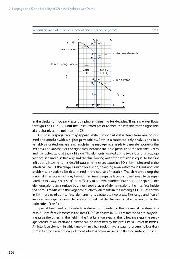
As given by [Wu, 2013], an inner seepage face may appear at an interface of two ma-terials inside the domain as shown in F.9-1. Because the seepage feature at the left side of Line EO in F.9-1 meets the condition of E.9-13, it can be named an inner seepage face. An inner seepage face is also a boundary between saturated and unsaturated areas like a free surface, with an essential feature difference that there is no flux flow out of a free surface in a saturated-only simulation, however, flux comes out of an inner seepage face and passes to the next zone. The mathematical expression of a free surface is given as:
00nq
ψ = =
E.9-15
Experimental results show that there is no liquid flow from a porous material with a higher saturation to a coarser material with a larger saturated permeability in an un-saturated area [Wang et al., 2003]. This principle is widely accepted and has been applied
200
9 Seepage and Slope Stability of Chinese Hydropower Dams
A GC
10 m
C'
B HD
F
Mk
Mj
O
E
Free surface
Inner seepage face
Zone 1k1
Zone 2k2 > k1
Free surface
Interface elements
M'k
M'j
Mi M'i
D'
2 m
Schematic map of interface element and inner seepage face F.9-1
in the design of nuclear waste dumping engineering for decades. Thus, no water flows through line CE in F.9-1 but the unsaturated pressure from the left side to the right side alters sharply at the point on line CE.
An inner seepage face may appear while unconfined water flows from one porous media to another with a higher permeability. Both in a saturated-only analysis and in a variably saturated analysis, each node in the seepage face needs two numbers, one for the left area and another for the right area, because the pore pressure at the left side is zero and it is below zero at the right side. The elements located at the two sides of a seepage face are separated in this way and the flux flowing out of the left side is equal to the flux infiltrating into the right side. Although the inner seepage face EO in F.9-1 is located at the interface line CD, the range is unknown a priori, changing even with time in transient flow problems. It needs to be determined in the course of iteration. The elements along the material interface which may be within an inner seepage face or above it need to be sepa-rated by this way. Because of the difficulty to put two numbers to a node and separate the elements along an interface by a mesh tool, a layer of elements along the interface inside the porous media with the larger conductivity, elements in the rectangle CDD’C’ as shown in F.9-1, are used as interface elements to separate the two areas. The range and flux of an inner seepage face need to be determined and the flux needs to be transmitted to the right side of the face.
Special treatment of the interface elements is needed in the numerical iteration pro-cess. All interface elements in the area CDD’C’ as shown in F.9-1 are treated as ordinary ele-ments as the others in the field in the first iteration step. In the following steps the seep-age feature of an interface element can be identified by the pressure values of its nodes. An interface element in which more than a half nodes have a water pressure no less than zero is treated as an ordinary element which is below or crossing the free surface. These el-
201
Numerical Method for Seepage Simulation and Slope Stability Analysis 9-2
ements need no special treatment. The other elements are on an inner seepage face or in an unsaturated area. These elements do not participate in the seepage coefficient tensor assemblage as expressed in E.9-5 at the next iteration step, thus separating the saturated and unsaturated area at the interface in the next iterative solution of the finite element equations. Nodes on the inner seepage face can be determined and their node flux can be obtained according to the procedure mentioned above. As shown in F.9-1, CE is a zero flux boundary, hence a node with a negative pressure needs no treatment for no water passes it to the downstream area. The EO is an inner seepage face boundary for zone 1 and the flux boundary for zone 2. The flux of a node on the inner seepage face needs to be added to the downstream area, e. g., the flux of node Mj adds to the opposite node M'j therefore the mass conservation law is abided. The flux which flows through the boundary EO is so small that the flow situation from the left side to the right side of the line is similar to the infiltration of dry soil. The relative conductivity at a Gaussian integral point in the element with a small infiltration flux in the two consecutive iteration steps changes suddenly dur-ing the iteration and the ratio of the conductivity between neighbouring Gaussian points at the element may be up to several orders of magnitude. This may cause poor iterative efficiency and serious divergent problems. To avoid this situation the total flux flow out of the seepage face EO can add to a line MkM'k which is proximal to the free surface at the downstream side.
All the undetermined boundary conditions including an inner seepage face condition are determined according to the pore water pressure obtained by the last iteration step in the course of the iteration. The procedure to deal with an inner seepage face problem is as follows:
1) An array should be set at first to store the node numbers of all nodes located at the interface and their attribute values, 1 for nodes below the seepage face which has a positive water pressure, 0 for nodes on the seepage face and –1 for nodes above the seepage face which has a negative pressure.
2) During the iteration, the fluxes of nodes on the seepage face need to be calculated according to E.9-12, the attribute values of those nodes which have a negative flux should be changed from 0 to –1 as a non-free surface node.
3) The attribute values of nodes with a positive pressure and –1 value need to be changed to 1 as a free surface node.
4) Interface elements where more than a half of the total element nodes are non-negative pore pressure nodes are marked as normal elements, non-normal elements do not participate in the seepage coefficient tensor assemblage at the next iteration step.
5) Nodes on the interface with 0 attribute value are treated as Dirichlet boundary nodes with 0 pore pressure and the flux of the nodes is added to downstream nodes as described in the previous paragraph.
202
9 Seepage and Slope Stability of Chinese Hydropower Dams
9-2-3 A Modified Gradient Procedure for Locating the Critical Slip Surface Based on Finite Element Stress Analysis
The choice of suitable methods of safety analysis is important. The direct finite ele-ment method can obtain both the factor of safety and information about the collapse mechanism [Naylor, 1982]. It is, however, not easy to obtain a factor of safety accurately within the confidence limits as achieved by limit equilibrium methods. A fine mesh is re-quired, a code capable of giving reliable results with the Mohr-Coulomb elastic-plastic model for loading states close to failure is needed, and finally it is usually necessary to carry out a set of analyses with load increased or the strength parameters c and tanϕ reduced progressively by a factor which will become the factor of safety when failure is eventually reached. These analyses become progressively more expensive as the factor of safety is increased.
Limit equilibrium methods provide a powerful means of evaluating safety. The cal-culation of stresses of the conventional limit equilibrium methods is based on slices. The assumptions about the distribution of stresses between slices have to be made by those methods. The impact of seepage on the effective stresses of a slope with complicated underground flow situations is difficult to be evaluated reliably by these methods. It is obvious that stresses from methods of slices may not agree with the actual ones in an unacceptably large extent in many situations, such as rock fill dams, foundations, river and water reservoir banks, and many slopes in rainy seasons. Meaningful stability analysis can be made only if the stress distribution within the structure can be predicted reliably [Clough and Woodward, 1967].
The assumptions related to the inter slice force in limit equilibrium methods are un-necessary when a finite element stress analysis is used. Kulhawy [Kulhawy, 1969] devel-oped a computer program to obtain an independent assessment of the normal and shear stresses along an assumed slip surface to calculate an overall factor of safety. Only one finite element analysis is required. The limit equilibrium methods based on finite element stresses analysis can be categorized as enhanced limit methods [Naylor, 1982]. They pro-vide an alternative way for obtaining the factor of safety. A case study shows that factors of safety computed when using the enhanced limit method are generally slightly lower than those computed using conventional limit equilibrium methods of slices [Pham and Fredlund, 2003]. Assumptions regarding the uncertainty of the shape of the critical slip surface can be omitted when an appropriate optimization technique is introduced into the analysis [Pham and Fredlund, 2003].
Optimization techniques have been developed by several researchers for over three decades and have provided a variety of approaches to determine the shape and location of the critical slip surface. Generally, optimization algorithms can be divided into two ba-sic classes: deterministic and heuristic algorithms. Deterministic methods [Baker, 1980; Baker and Garber, 1978; Bardet and Kapuskar, 1989; Celestino and Duncan, 1981; Chen and Shao, 1988; Nguyen, 1985; Menon et al., 2001] are based on the gradient informa-tion of the objective function and constraints, they may lead to a false critical slip surface due to the presence of several local minima points over the solution domain [Chen and Shao, 1988; McCombie and Wilkinson, 2002; Taha et al., 2010]. Heuristic approaches, in-cluding several algorithms such as genetic algorithms, simulated annealing, Tabu search,
203
Numerical Method for Seepage Simulation and Slope Stability Analysis 9-2
τσn
P1 (entrance point)
P2 (exit point)
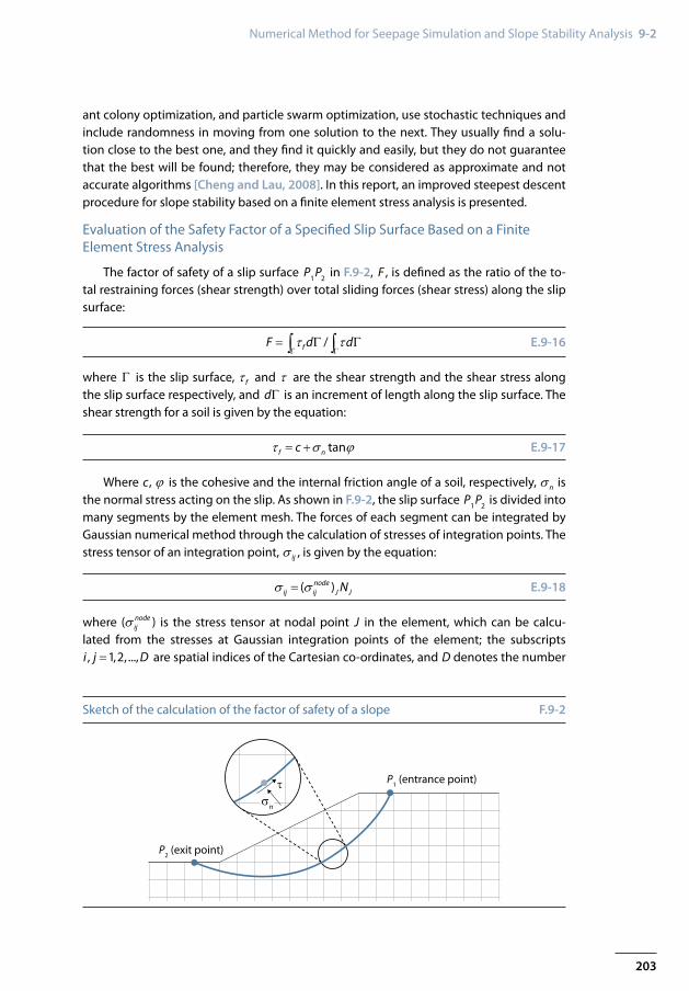
Sketch of the calculation of the factor of safety of a slope F.9-2
ant colony optimization, and particle swarm optimization, use stochastic techniques and include randomness in moving from one solution to the next. They usually find a solu-tion close to the best one, and they find it quickly and easily, but they do not guarantee that the best will be found; therefore, they may be considered as approximate and not accurate algorithms [Cheng and Lau, 2008]. In this report, an improved steepest descent procedure for slope stability based on a finite element stress analysis is presented.
Evaluation of the Safety Factor of a Specified Slip Surface Based on a Finite Element Stress Analysis
The factor of safety of a slip surface P1P2 in F.9-2, F , is defined as the ratio of the to-tal restraining forces (shear strength) over total sliding forces (shear stress) along the slip surface:
/fF d dτ τΓ Γ
= Γ Γ∫ ∫ E.9-16
where Γ is the slip surface, fτ and τ are the shear strength and the shear stress along the slip surface respectively, and dΓ is an increment of length along the slip surface. The shear strength for a soil is given by the equation:
tanf ncτ σ ϕ= + E.9-17
Where c, ϕ is the cohesive and the internal friction angle of a soil, respectively, nσ is the normal stress acting on the slip. As shown in F.9-2, the slip surface P1P2 is divided into many segments by the element mesh. The forces of each segment can be integrated by Gaussian numerical method through the calculation of stresses of integration points. The stress tensor of an integration point, ijσ , is given by the equation:
( )nodeij ij J JNσ σ= E.9-18
where ( )nodeijσ is the stress tensor at nodal point J in the element, which can be calcu-
lated from the stresses at Gaussian integration points of the element; the subscripts , 1,2, ...,i j D= are spatial indices of the Cartesian co-ordinates, and D denotes the number
204
9 Seepage and Slope Stability of Chinese Hydropower Dams
of spatial dimension (2 or 3); NJ is the shape function of the point at nodal J of the ele-ment; summation convention is used for repeated indices. The shape function N can be calculated directly from the local coordinates which can be transformed from the global coordinates of the point according to the numerical inverse iso-parametric mapping method [Murti and Valliappan, 1986].
The stress vector of an integrated point at the slip surface, Ti , can be calculated from the stress tensor of the point as follows:
i ij jT nσ= E.9-19
where nj is the unit vector of the normal direction of the slip surface at the point. The nor-mal and shear stresses of the point can be calculated as follows:
n i iT nσ = E.9-20
i iT lτ = E.9-21
where li is the unit vector of the tangent direction of the curve at the point. The total re-straining or sliding force in E.9-16 is the sum of the force of all the curve segments. Thus the factor of safety of the slip surface can be obtained from E.9-16 ~ E.9-21.
Modified Gradient Method
Finding the critical slip surface related to the minimum factor of safety, Fmin , involves a mathematical procedure for minimizing the factor of safety function F(Z) of the slip sur-face expressed by a certain mathematical pattern and the vector 1 2( , , ..., )nz z zZ formed by a set of geometric variables 1 2( , , ..., )nz z z .
The search process starts from an initial slip surface 0 0 0 01 2( , , ..., )nz z zZ and terminates at
a location with the factor of safety Fmin. Different choices of the initial slip surface will not affect the solution unless the problem exhibits multi-minima behaviour. The slip surface position with the minimum factor of safety locates at the range boundary of the vector Z or at a minimum point where the gradient vector G equals zero as stated as:
,1 ,2 ,( , , ..., ) 0nF F F =G E.9-22
For the current step at iteration m with the slip surface mZ moves to the next position 1m+Z with respect to a step coefficient α and a certain direction vector S, and it may be
anticipated that the factor of safety at the new position will be smaller.
1m m mα+ = +Z Z S E.9-23
The steepest descent method defines the minimizing direction S as the negative of the gradient vector G, that is:
,1 ,2 ,( , , , )nF F F= − = − S G E.9-24
205
Numerical Method for Seepage Simulation and Slope Stability Analysis 9-2
2.0
1.9
1.8
1.81.7
2.0
1.9
1.8
1.8
1.7A
A1
P2
P1
A'
A'1
C
B
A
P2
P1
C
B
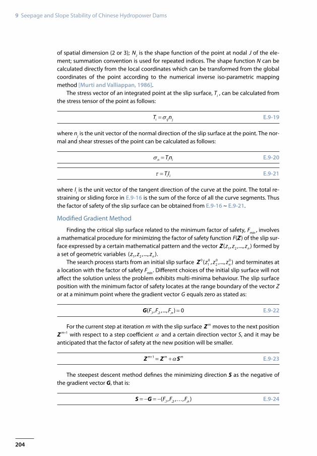
Sketch of the steepest descent search method: classic method (left) and modified method (right)
F.9-3
In the classic method, the determination of the α value is through the solution of the following equation [Chen and Shao, 1988].
[ ( )] 0m mFF α
α α∂ ∂
= + =∂ ∂
Z S E.9-25
A modified method is proposed in this study. A fixed small α value is used directly in E.9-23 other than to solve E.9-25 to find the minimum point along the direct vector in the whole domain. The value of the objective function will undergo a steady reduction along the negative gradient direction approximately as shown in F.9-3 (right). If the objective value of the tentative position is not decreased compared with the previous point, 1( ) ( )m mF F+ ≥Z Z , the function across the space of the search step must undergo a process of decreasing to increasing from mZ to 1m+Z , illustrated that there is a minimum in the range 1[ , ]m m+Z Z along the line. Single variable optimization can be used to determine the minimum point position and take this position as the new start in the next step. The minimum points P1 and P2 have been found out according to the modified method. The search point in the modified method moves forward approximately according to the steepest descent direc-tion. Hence it is a veritable down-hill method. The contours information of the objective function can be figured out from a group of search routes, therefore the global minimum can be obtained.
Normalization of the domain of each variable to [0, 1] and normalization of the direc-tion vector except when it is equal to zero can make the choice of the search step coef-ficient α easy and independent of the geometric size of the problem. Given the range of the control variable of the sliding surface zi as min max[ , ]i iz z , the normalization equation of the variable is
min max min( ) / ( )i i i i iz z z z z= − − E.9-26
The tentative new slip surface position vector 1m+Z based on the current step vector mZ is defined as

206
9 Seepage and Slope Stability of Chinese Hydropower Dams
F
A
zi
( ) / ( ) /m mi iD F
F z z F z z∂ ∂ = ∂ ∂
miz δ− m
iz δ+ miz
( )m
i F
F zz
∂∂
( )m
i M
F zz
∂∂
F
B
zi
( ) / ( ) /m mi iD B
F z z F z z∂ ∂ = ∂ ∂
miz δ− m
iz δ+ miz
( )m
i B
F zz
∂∂
( )m
i M
F zz
∂∂
F
Descent forward Descent backward Descent neither forward nor backward
zi miz δ− m
iz δ+ miz
( )m
i B
F zz
∂∂
( )m
i F
F zz
∂∂
( )m
i M
F zz
∂∂
( ) / 0mi D
F z z∂ ∂ =
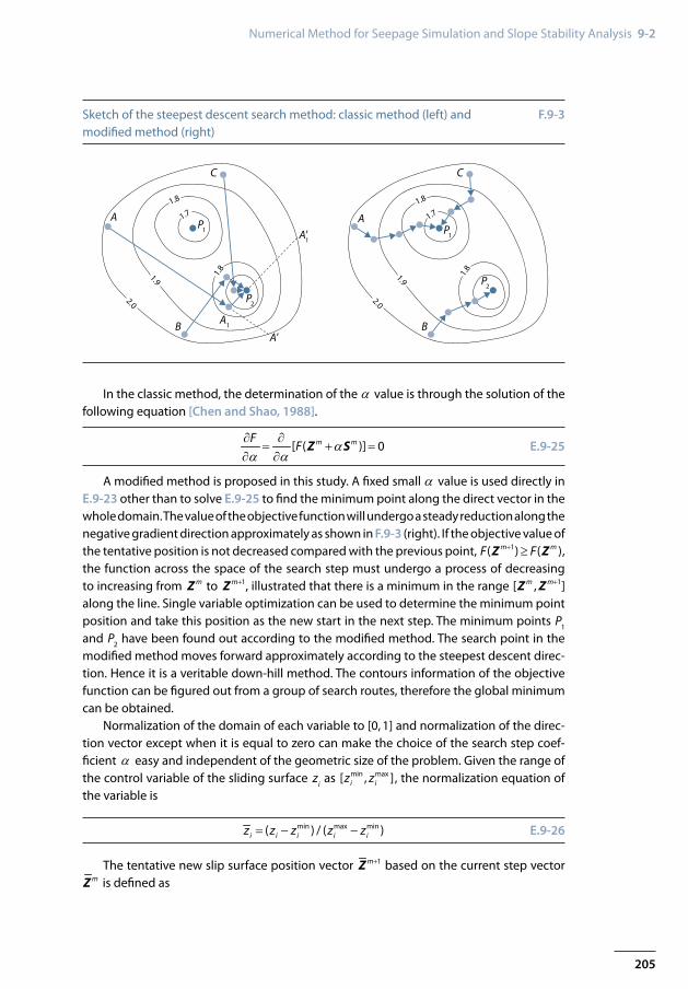
Sketch of the descent difference scheme: descent forward (left); descent backward (middle); descent neither forward nor backward (right)
F.9-4
1m m mα+ = +Z Z S E.9-27
where mS is the normalized direction vector, 2
/m m m= −S G G . If the direction vector is equal to zero ( 0)m =S according to the descent difference
scheme introduced in the next section, a minimum point must be located in the approxi-mate δ neighbourhood of the point mZ . One dimensional optimization could be used for variable zi , 1, ,i n= , in interval [ , ]m m
i iδ δ− +Z e Z e , the minimum location could be found after several times of the single variable optimization. In order to avoid that a search falls into a pit, the range of single variable optimization is recommended to broaden to [ , ]m m
i iβ β− +Z e Z e (β equal to α is usually a good choice), if the minimum value is lo-cated outside the range [ , ]m m
i iδ δ− +Z e Z e , the minimum in the δ neighbourhood of point mZ is a local minimum which can be ignored and the search should continue with the new point.
Difference Scheme for the Partial Derivative of the Objective Function
It is generally recognized that either forward or backward difference is unfit for the calculation of the director vector, for the vector obtained via these methods may be the opposite direction of the actual descent direction near the extreme point [Chen, 2003; Zhu et al., 1984]. Central difference is generally used to calculate the vector. However, the direction vector calculated by the central difference scheme drifts off the true negative gradient at a point where the objective function is not linearly changed with the coordi-nate in the δ (δ is the difference step) neighbourhood of the point. The objective function is non-linear at areas where the contours of the function form a trench or at concave area where a minimum exists, the direction vector obtained differs from the steepest descent direction greatly. The search usually terminates at a point just close to the minimum, but not the exact position. The direction vector may even point to a rising direction and thus terminates the search process at a false minimum. A descent difference scheme is pre-sented as shown in F.9-4. The descent difference value is equal to the forward difference at situation (left), equal to the backward difference at situation (middle), and is set to zero at situation (right). As a matter of fact, compared with the central difference, the descent
207
Numerical Method for Seepage Simulation and Slope Stability Analysis 9-2
difference value is closer to the steepest descent direction of the function if the function is monotonous among the range [ , ]m m
i iδ δ− +Z e Z e as shown in F.9-4 (left) and (middle), where ei is the unit vector along the coordinate axis i and δ is the difference step.
The descent difference scheme is given by the equation:
( ) / , ( ) ( ) ( )
( ) / ( ) / , ( ) ( ) ( )
0, ( ) ( ) ( )
m m m mi i iF
m m m m mi i i iD B
m m mi i
F z z F F F
F z z F z z F F F
F F F
δ δ
δ δ
δ δ
∂ ∂ − > > +∂ ∂ = ∂ ∂ − < < +
− ≥ ≤ +
Z e Z Z e
Z e Z Z e
Z e Z Z e
E.9-28
where, ( ) /mi F
F z z∂ ∂ and ( ) /mi B
F z z∂ ∂ are the forward and backward differences, respec-tively. They are calculated by the following formulae.
( ) / [ ( ) ( )] /m m mi iF
F z z F Fδ δ∂ ∂ = + −Z e Z E.9-29
( ) / [ ( ) ( )] /m m mi iB
F z z F F δ δ∂ ∂ = − −Z Z e E.9-30
The calculation of the partial difference at point mZ along the axis i starts with a guess of the descent direction. The descent direction of the last step is used as the guess. The value ( )m
iF δ+Z e at descent forward guess or ( )miF δ−Z e at descent backward guess is
calculated. Then the actual descent direction can be checked via the comparison of the obtained value with ( )mF Z . If the guess is right, the descent difference can be calculated like the last step, otherwise, the factor of safety of the point at the other side of mZ along the axis should be calculated and the partial difference value can be calculated according to E.9-28. The number of times of the calculation of the factor of safety is 1n+ in a moving step in case of right guess which is usually the situation while a small moving step coef-ficient is adopted, whereas the number in a central difference scheme is 2 1n+ .
Error Estimation and Convergence Criterion
An error estimation is a necessary but often overlooked item in a non-linear optimiza-tion. As given by [Chen and Shao, 1988], the optimization terminates at the condition stated as:
1( ) ( )m mF F ε−− ≤Z Z E.9-31
where, ε is a tiny value used to be taken as 1.0×10⁻⁵. The actual deviation of the cur-rent factor of safety to the minimum values may be far greater than the given value, ε ,
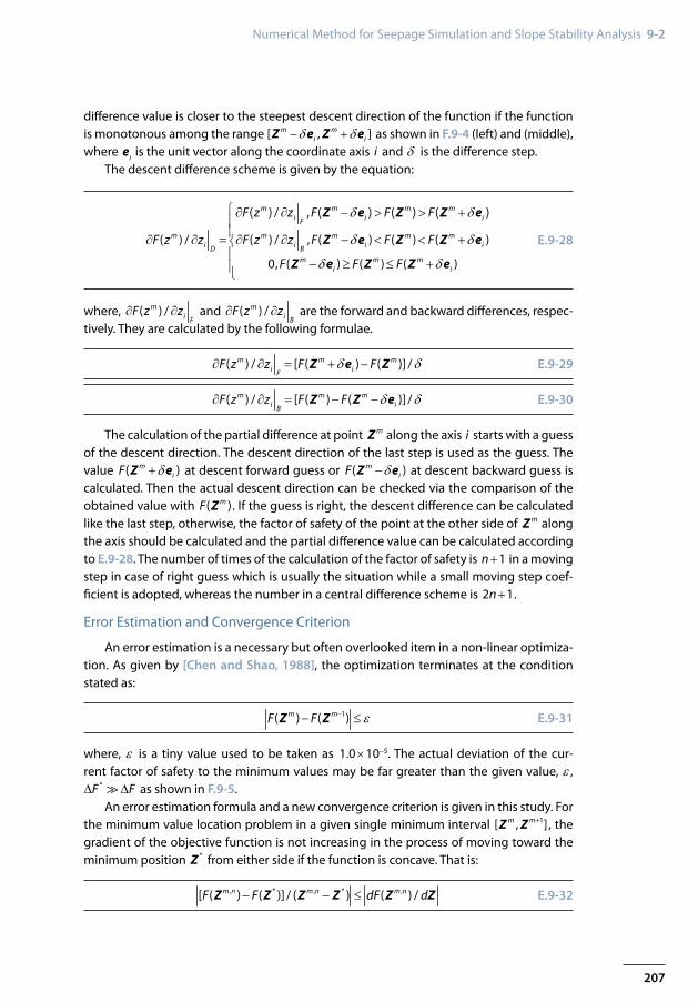
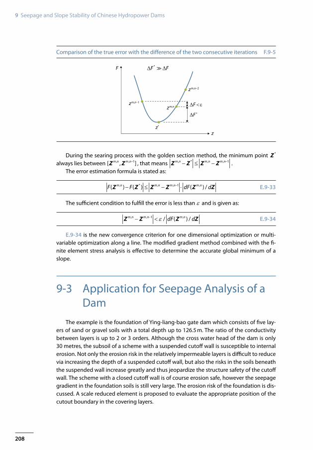
*F F∆ ∆ as shown in F.9-5.An error estimation formula and a new convergence criterion is given in this study. For
the minimum value location problem in a given single minimum interval 1[ , ]m m+Z Z , the gradient of the objective function is not increasing in the process of moving toward the minimum position *Z from either side if the function is concave. That is:
, * , * ,[ ( ) ( )] / ( ) ( ) /m n m n m nF F dF d− − ≤Z Z Z Z Z Z E.9-32
208
9 Seepage and Slope Stability of Chinese Hydropower Dams
*F F∆ ∆F
zz*
∆F *
∆F <εzm,nzm,n−1
zm,n−2
Comparison of the true error with the difference of the two consecutive iterations F.9-5
During the searing process with the golden section method, the minimum point *Z always lies between , , 1[ , ]m n m n−Z Z , that means , * , , 1m n m n m n−− ≤ −Z Z Z Z .
The error estimation formula is stated as:
, * , , 1 ,( ) ( ) ( ) /m n m n m n m nF F dF d−− ≤ − ⋅Z Z Z Z Z Z E.9-33
The sufficient condition to fulfill the error is less than ε and is given as:
, , 1 ,/ ( ) /m n m n m ndF dε−− <Z Z Z Z E.9-34
E.9-34 is the new convergence criterion for one dimensional optimization or multi-variable optimization along a line. The modified gradient method combined with the fi-nite element stress analysis is effective to determine the accurate global minimum of a slope.
9-3 Application for Seepage Analysis of a Dam
The example is the foundation of Ying-liang-bao gate dam which consists of five lay-ers of sand or gravel soils with a total depth up to 126.5 m. The ratio of the conductivity between layers is up to 2 or 3 orders. Although the cross water head of the dam is only 30 metres, the subsoil of a scheme with a suspended cutoff wall is susceptible to internal erosion. Not only the erosion risk in the relatively impermeable layers is difficult to reduce via increasing the depth of a suspended cutoff wall, but also the risks in the soils beneath the suspended wall increase greatly and thus jeopardize the structure safety of the cutoff wall. The scheme with a closed cutoff wall is of course erosion safe, however the seepage gradient in the foundation soils is still very large. The erosion risk of the foundation is dis-cussed. A scale reduced element is proposed to evaluate the appropriate position of the cutout boundary in the covering layers.
209
Application for Seepage Analysis of a Dam 9-3
134014
00
1400
1300
1300
1300
1300
1240
1240
1240
1240
1240
126012
20
-200 0 200 400 600X /m
-400
-200
0
200
400
600
Y /m
CFRD
Y=0+000
Y=0+250
X=0+
000
X=0+
000
X=0+
050
X=0+
170
Y=0−070
DaduRiver
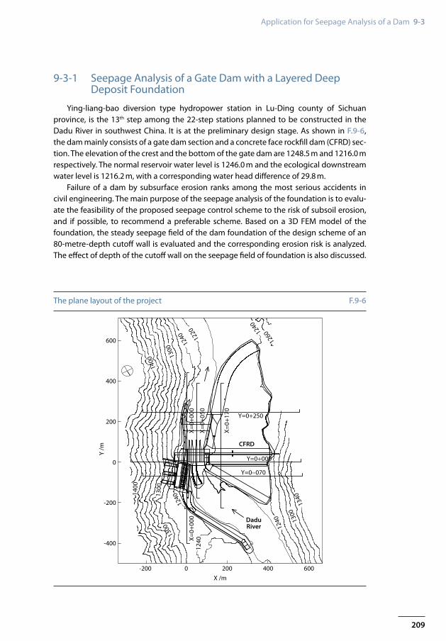
The plane layout of the project F.9-6
9-3-1 Seepage Analysis of a Gate Dam with a Layered Deep Deposit Foundation
Ying-liang-bao diversion type hydropower station in Lu-Ding county of Sichuan province, is the 13th step among the 22-step stations planned to be constructed in the Dadu River in southwest China. It is at the preliminary design stage. As shown in F.9-6, the dam mainly consists of a gate dam section and a concrete face rockfill dam (CFRD) sec-tion. The elevation of the crest and the bottom of the gate dam are 1248.5 m and 1216.0 m respectively. The normal reservoir water level is 1246.0 m and the ecological downstream water level is 1216.2 m, with a corresponding water head difference of 29.8 m.
Failure of a dam by subsurface erosion ranks among the most serious accidents in civil engineering. The main purpose of the seepage analysis of the foundation is to evalu-ate the feasibility of the proposed seepage control scheme to the risk of subsoil erosion, and if possible, to recommend a preferable scheme. Based on a 3D FEM model of the foundation, the steady seepage field of the dam foundation of the design scheme of an 80-metre-depth cutoff wall is evaluated and the corresponding erosion risk is analyzed. The effect of depth of the cutoff wall on the seepage field of foundation is also discussed.
210
9 Seepage and Slope Stability of Chinese Hydropower Dams
Scale reduced elements
Scale reduced elements
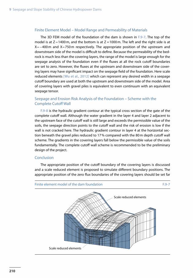
Finite element model of the dam foundation F.9-7
Finite Element Model – Model Range and Permeability of Materials
The 3D FEM model of the foundation of the dam is shown in F.9-7. The top of the model is at Z =1400 m, and the bottom is at Z = 1000 m. The left and the right side is at X= −400 m and X=750 m respectively. The appropriate position of the upstream and downstream side of the model is difficult to define. Because the permeability of the bed-rock is much less than the covering layers, the range of the model is large enough for the seepage analysis of the foundation even if the fluxes at all the rock cutoff boundaries are set to zero. However, the fluxes at the upstream and downstream side of the cover-ing layers may have significant impact on the seepage field of the foundation. Here scale reduced elements [Wu et al., 2012] which can represent any desired width in a seepage cutoff boundary are used at both the upstream and downstream side of the model. Area of covering layers with gravel piles is equivalent to even continuum with an equivalent seepage tensor.
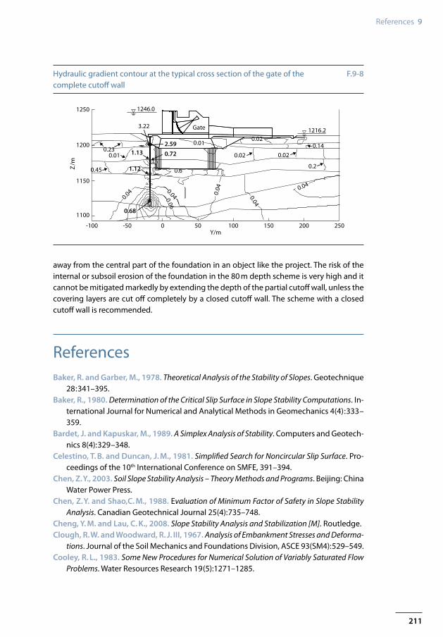
Seepage and Erosion Risk Analysis of the Foundation – Scheme with the Complete Cutoff Wall
F.9-8 is the hydraulic gradient contour at the typical cross section of the gate of the complete cutoff wall. Although the water gradient in the layer 4 and layer 2 adjacent to the upstream face of the cutoff wall is still large and exceeds the permissible value of the soils, the seepage direction points to the cutoff wall and the risk of erosion is low if the wall is not cracked here. The hydraulic gradient contour in layer 4 at the horizontal sec-tion beneath the gravel piles reduced to 17 % compared with the 80 m depth cutoff wall scheme. The gradients in the covering layers fall below the permissible value of the soils fundamentally. The complete cutoff wall scheme is recommended to be the preliminary design of the project.
Conclusion
The appropriate position of the cutoff boundary of the covering layers is discussed and a scale reduced element is proposed to simulate different boundary positions. The appropriate position of the zero flux boundaries of the covering layers should be set far
211
References 9
1250
Z/m
Y/m
1200
-100 -50 0 50 100 150 200 250
1100
1150
2.59
0.72
0.68
1.13
1.12
1246.0
1216.2Gate
0.23
0.45
0.01
3.22
0.01
0.040.04
0.06
0.6
0.02 0.02
0.2
0.140.02
0.04 0.04
0.04
Hydraulic gradient contour at the typical cross section of the gate of the complete cutoff wall
F.9-8
away from the central part of the foundation in an object like the project. The risk of the internal or subsoil erosion of the foundation in the 80 m depth scheme is very high and it cannot be mitigated markedly by extending the depth of the partial cutoff wall, unless the covering layers are cut off completely by a closed cutoff wall. The scheme with a closed cutoff wall is recommended.
ReferencesBaker, R. and Garber, M., 1978. Theoretical Analysis of the Stability of Slopes. Geotechnique
28:341–395.Baker, R., 1980. Determination of the Critical Slip Surface in Slope Stability Computations. In-
ternational Journal for Numerical and Analytical Methods in Geomechanics 4(4):333–359.
Bardet, J. and Kapuskar, M., 1989. A Simplex Analysis of Stability. Computers and Geotech-nics 8(4):329–348.
Celestino, T. B. and Duncan, J. M., 1981. Simplified Search for Noncircular Slip Surface. Pro-ceedings of the 10th International Conference on SMFE, 391–394.
Chen, Z. Y., 2003. Soil Slope Stability Analysis – Theory Methods and Programs. Beijing: China Water Power Press.
Chen, Z. Y. and Shao,C. M., 1988. Evaluation of Minimum Factor of Safety in Slope Stability Analysis. Canadian Geotechnical Journal 25(4):735–748.
Cheng, Y. M. and Lau, C. K., 2008. Slope Stability Analysis and Stabilization [M]. Routledge.Clough, R. W. and Woodward, R. J. III, 1967. Analysis of Embankment Stresses and Deforma-
tions. Journal of the Soil Mechanics and Foundations Division, ASCE 93(SM4):529–549.Cooley, R. L., 1983. Some New Procedures for Numerical Solution of Variably Saturated Flow
Problems. Water Resources Research 19(5):1271–1285.
212
9 Seepage and Slope Stability of Chinese Hydropower Dams
Kulhawy, F. H., 1969. Finite Element Analysis of the Behaviour of Embankments. PhD Thesis, University of California, Berkley, California, USA.
McCombie, P. and Wilkinson, P., 2002. The Use of the Simple Genetic Algorithm in Find-ing the Critical Factor of Safety in Slope Stability Analysis. Computers and Geotechnics 29(8):699–714.
Menon et al., 2001. Mualem, Y., 1976. A New Model for Predicting the Conductivity of Unsaturated Porous Media.
Water Resources Research 12:513–522.Murti, V. and Valliappan, S., 1986. Numerical Inverse Isoparametric Mapping in Remeshing
and Nodal Quantity Contouring. Computers & Structures 22(6):1011–1021.Naylor, D. L., 1982. Finite Elements and Slope Stability. In Numerical Methods in Geome-
chanics, D. Reidel Publishing Company, J. B. Martins (eds), 229–244.Nguyen, V. U, 1985. Determination of Critical Slope Failure Surface. J. Geotech. Eng., ASCE
111(2):238–250.Pham, H. T. V. and Fredlund, D. G., 2003. The Application of Dynamic Programming to Slope
Stability Analysis. Canadian Geotechnical Journal 40:830–847.Richards, L. A., 1931. Capillary Conduction of Liquids through Porous Mediums. Physics 1:
318–333.Taha., M. R., Khajehzadeh, M. and EI-Shafie, A., 2010. Slope Stability Assessment Using
Optimization Techniques: an Overview. Electronic Journal of Geotechnical Engineering 15(R):1901–1915.
Van Genuchten, M. Th., 1980. A Closed-Form Equation for Predicting the Hydraulic Conduc-tivity of Unsaturated Soils. Soil Science Society of America Journal 44:892–898.
Wang, Z. M., Jiang, H., Yao, L., et al., 2003. Qualitative Experiment of Unsaturated Water Vadose through Two-Layer Porous Media. Radiat Prot 23(1):8–13.
Wu, M. X. and Gao, L. S., 1999. Numerical Simulation of Saturated-Unsaturated Transient Flow in Soils. Journal of Hydraulic Engineering (Chinese) 1999(12):38–42.
Wu, M. X., 2010. A Finite-Element Algorithm for Modeling Variably Saturated Flows. Journal of Hydrology, 394(3–4):315–323.
Wu, M. X., Yang, L. Z. and Hu, X. H., 2012. Seepage Analysis of a Gate Dam with a Layered Deep Deposit Foundation. Proceedings of the Third International Symposium on Life Cycle Civil Engineering, Hofburg Palace, Vienna, Austria, 3–6 October 2012.
Wu, M. X., Yang, L. Z. and Yu, T., 2013. Simulation Procedure of Unconfined Seepage with an Inner Seepage Face in a Heterogeneous Field. Science China Physics, Mechanics & Astronomy 56(6):1139–1147.
Zhang, X. X., Glyn Bengough, A., Crawford, J. W. and Young, I. M., 2002. Efficient Methods for Solving Water Flow in Variably Saturated Soils under Prescribed Flux Infiltration. Jour-nal of Hydrology 260:75–87.
Zhu, B. F., Li, Z. M. and Zhang, B. C., 1984. Principles and Applications of Optimal Structure Designing [M]. Beijing: Water conservancy and electric power press.