Marine Chemistry 161 (2014) 1–13

Contents lists available at ScienceDirect

Marine Chemistry

j ourna l homepage: www.e lsev ie r .com/ locate /marchem

Seasonal variability of aragonite saturation state in the Western Pacific

Mareva Kuchinke a,⁎, Bronte Tilbrook a,b,c, Andrew Lenton a

a Centre for Australian Weather and Climate Research, CSIRO Marine and Atmospheric Research, Hobart, Tasmania, Australiab CSIROWealth from Oceans National Research Flagship, PO Box 1538, Hobart, TAS 7001, Australiac Antarctic Climate and Ecosystems CRC, Hobart, TAS 7001, Australia

⁎ Corresponding author.E-mail address: mkuchinke@gmail.com (M. Kuchinke)

http://dx.doi.org/10.1016/j.marchem.2014.01.0010304-4203/Crown Copyright © 2014 Published by Elsevie

a b s t r a c t

a r t i c l e i n f o

Article history:Received 24 May 2013Received in revised form 19 December 2013Accepted 7 January 2014Available online 24 January 2014

Keywords:Aragonite saturation stateSeasonal variabilitySurface tropical Pacific OceanProcessesPrecipitationAdvectionUpwelling

The oceanic uptake of atmospheric carbon dioxide (CO2) since pre-industrial times has increased acidity levels,resulting in a decrease in the pH and aragonite saturation state (Ωar) of surface waters. Aragonite is the predom-inant biogenic form of calcium carbonate precipitated by calcifying organisms in tropical reef ecosystems. ValuesofΩar are often used as a proxy for estimating calcification rates in corals and other calcifying species. We quan-tify the regional and seasonal variability of Ωar and its main drivers for the Pacific island region (120°E:140°W,35°S:30°N). The calculation ofΩar uses a seasonal climatology of the surface-water partial pressure of CO2, com-bined with values of total alkalinity (TA) estimated from a relationship between surface water salinity and totalalkalinity that is derived from measurements in the region. This relationship is valid for all phases of El Niño/Southern Oscillation and for mixed layer waters with less than 15 μmol kg−1 dissolved nitrate.The influence of seasonal changes in sea surface temperature (SST) onΩar is small except in the subtropical wa-ters on the northern and southern boundaries of the study region. Here, SST seasonal variability is large (N5 °C),causing a change inΩar of greater than 0.1. Seasonal changes in mixed layer depth and net evaporation (precip-itation) do influence the seasonality in TCO2 and TA. However, these processes tend to increase (decrease) theTCO2 (TA) in unison, resulting in a small net effect on seasonal change inΩar formost of the region. Net biologicalproduction and sea–air gas exchange were also found to have only a small impact on the seasonal change inΩar

through the region. Changes inΩar of between 0.1 and 0.2 occurredwhere variations inwind-driven upwelling inthe Central Equatorial Pacific and the transport of Eastern Pacific waters into the South Equatorial Current regioncaused a change in the TCO2/TA ratio of the surface waters. In contrast to these two regions, the combined effectof biological and physical processes in theWest Pacific Warm Pool and North Equatorial Counter Current subre-gions resulted inΩar variability of less than 0.1.Crown Copyright © 2014 Published by Elsevier B.V. This is an open access article under the CC BY-NC-SA license

(http://creativecommons.org/licenses/by-nc-sa/3.0/).

1. Introduction

Since the start of the industrial revolution, about 48% of the anthro-pogenic CO2 emitted to the atmosphere has been taken up and stored inthe ocean (Sabine et al., 2004). The CO2 taken up by the ocean reacts inseawater, causing decreases in pH and dissolved carbonate ion concen-trations (CO3

2−), with the changes collectively referred to as oceanacidification (e.g. Caldeira and Wickett, 2003).

Ocean acidification is expected to reduce calcification in reefecosystems (Hoegh-Guldberg et al., 2007; Langdon et al., 2000; Orret al., 2005), may alter nutrient speciation and availability (Doreet al., 2009), and potentially change phytoplankton species composi-tion and growth (Fabry et al., 2008; Iglesias-Rodriguez et al., 2008).Many marine calcifying organisms such as corals, calcareous algae,and mollusks, tend to exhibit a reduced capacity to build their shellsand skeletons under more acidic conditions (Doney et al., 2012).

.

r B.V. This is an open access article u

Ocean acidification, in conjunction with additional stresses such asocean warming, has implications for the health and longer-termsustainability of reef ecosystems (Silverman et al., 2009) with poten-tial to impact fisheries, aquaculture, tourism, and coastal protection(e.g. Cooley et al., 2009).

In the tropical Pacific Ocean, the increase of atmospheric CO2 concen-trations for the period 1750–1995 is estimated to have resulted in a de-crease in surface water CO3

2− from ~270 μmol kg−1 to ~225 μmol kg−1

(Feely et al., 2009). For a high CO2 emission scenario such as A2(Nakicenovic et al., 2000), the atmospheric CO2 concentration is predictedto be about 850 ppm by 2100, which is projected to lead to a decrease inCO3

2− to ~140 μmol kg−1 (Feely et al., 2009).The decrease in the dissolved carbonate ion concentration that oc-

curs through ocean acidification results in a decrease in the aragonitesaturation state (Ωar) of the waters:

Ωar ¼Ca2þh i

Co2−3h i

K�sp

ð1Þ

nder the CC BY-NC-SA license (http://creativecommons.org/licenses/by-nc-sa/3.0/).

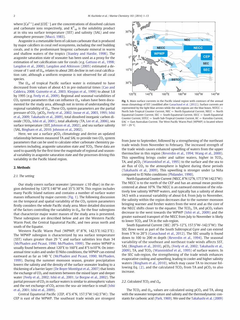
Fig. 1. Main surface currents in the Pacific island region with contours of the annualmean climatology of SST (modified after Ganachaud et al. (2012)). Surface currents arerepresented by the light blue arrows while the sub-regions are the blue boxes. NSTCC =North Sub-Tropical Counter Current, NEC = North Equatorial Current, NECC = NorthEquatorial Counter Current, SEC = South Equatorial Current, SECC = South EquatorialCounter Current, SSTCC = South Sub-Tropical Counter Current, KC = Kuroshio Current,EAC = East Australian Current. The West Pacific Warm Pool (WPWP) is located whereSST N 29 °C.

2 M. Kuchinke et al. / Marine Chemistry 161 (2014) 1–13

where [Ca2+] and [CO32−] are the concentrations of dissolved calcium

and carbonate ions respectively, and K⁎sp is the solubility productat in situ sea surface temperature (SST) and salinity (SAL) and oneatmosphere pressure (Mucci, 1983).

Aragonite is ametastable form of calcium carbonate that is producedby major calcifiers in coral reef ecosystems, including the reef buildingcorals, and is the predominant biogenic carbonate mineral in warmand shallow waters of the tropics (Stanley and Hardie, 1998). Thearagonite saturation state of seawater has been used as a proxy for theestimation of net calcification rate for corals (e.g. Gattuso et al., 1998;Langdon et al., 2000). Langdon and Atkinson (2005) estimated a de-crease of 1 unit ofΩar relates to about 28% decline in net coral calcifica-tion rate, although a uniform response is not observed for all coralspecies.

The Ωar of tropical Pacific surface water is estimated to havedecreased from values of about 4.5 in pre-industrial times (Cao andCaldeira, 2008; Guinotte et al., 2003; Kleypas et al., 1999) to about 3.8by 1995 (e.g. Feely et al., 2009). Regional and seasonal variabilities ofCO2 system parameters that can influence Ωar values have been docu-mented for the study area, although not in terms of understanding theregional variability of Ωar. These CO2 system parameters are the partialpressure of CO2 (pCO2, Feely et al., 2002; Inoue et al., 2003, 1995; Ishiiet al., 2009; Takahashi et al., 2009), total dissolved inorganic carbon di-oxide (TCO2, Ishii et al., 2001), total alkalinity (TA, Lee et al., 2006), seasurface temperature (SST, Johnson et al., 2002), and sea surface salinity(SAL, Bingham et al., 2010; Johnson et al., 2002).

Here, we use a surface pCO2 climatology and derive an updatedrelationship between measured TA and SAL to provide two CO2 systemparameters that can be used to calculate other carbonate chemistry pa-rameters including, aragonite saturation state and TCO2. These data areused to quantify for the first time themagnitude of regional and season-al variability in aragonite saturation state and the processes driving thisvariability in the Pacific Island region.

2. Methods

2.1. The setting

Our study covers surface seawater (pressure ≤10 dbar) in the re-gion delimited by 120°E:140°W and 35°S:30°N. This region includesmany Pacific Island nations and contains a number of surface watermasses influenced by major currents (Fig. 1). The following discussionon the temporal and spatial variability of the CO2 system parametersfirstly considers the whole Pacific study area. More detailed discussionof the factors controlling the variability in Ωar for the four subregionsthat characterize major water masses of the study area is presented.These subregions are described below and are the Western PacificWarm Pool, the Central Equatorial Pacific, and two areas north andsouth of the Equator.

Western Pacific Warm Pool (WPWP, 0°:8°N, 142.5°E:162.5°E):The WPWP subregion is characterized by sea surface temperature(SST) values greater than 29 °C and surface salinities less than 34(McPhaden and Picaut, 1990; McPhaden, 1999). The entire WPWP isusually found between about 120°E to 160°E and 8°S to10°N. On inter-annual time scales and under El Niño conditions, theWPWP can extendeastward as far as 140 °C (McPhaden and Picaut, 1990; McPhaden,1999). During the summer monsoon season, greater precipitationlowers the salinity and the density of the surface seawater leading to athickening of a barrier layer (De BoyerMontégut et al., 2007) that limitsthe exchange of CO2 and nutrients between themixed layer and deeperwater (Feely et al., 2002; Ishii et al., 2001; Le Borgne et al., 2002). Thepartial pressure of CO2 in surfacewaters is similar to atmospheric valuesand the net exchange of CO2 across the sea–air interface is small (Ishiiet al., 2001; Ishii et al., 2009).

Central Equatorial Pacific (CEP, 4°S:4°N, 157.5°W:142.5°W): TheCEP is east of the WPWP. The southeast trade winds are strongest

from June to September, followed by a strengthening of the northeasttrade winds from November to February. The increased strength ofthe trade winds causes enhanced upwelling of waters from the upperthermocline in this region (Reverdin et al., 1994; Wang et al., 2000).This upwelling brings cooler and saltier waters, higher in TCO2,TA, and pCO2 (Wanninkhof et al., 1995) to the surface and the sea toair flux of CO2 to the atmosphere is highest during these periods(Takahashi et al., 2009). This upwelling is stronger under La Niñacompared to El Niño conditions (Philander, 1990).

NorthEquatorial CounterCurrent (NECC, 8°N:12°N, 177.5°W:142.5°W):The NECC is to the north of the CEP and has an annual mean positioncentered at about 10°N. The NECC is an eastward extension of the rela-tively low salinity WPWP waters, and typically has a salinity of about34.5 with a seasonal variability of about 0.4. From July to November,the salinity within the region decreases due to the summer monsoonbringing warmer and fresher waters from the west and as the core ofthe NECC shifts closer to the equator. The TCO2, TA, and pCO2 valuesdecrease to the west towards the WPWP (Ishii et al., 2009) and thegreater eastward transport of the NECC from July to November is likelyto lower TCO2 and TA in the sub-region.

South Equatorial Current (SEC: 20°S–12°S, 157.5°W–142.5°W): TheSEC flows west as part of the South Subtropical Gyre and can extendfrom 5°N to 20°S (Ganachaud et al., 2012). The SEC usually is founddown to 100 to 200 m depth (Reverdin et al., 1994). The seasonalvariability of the southeast and northeast trade winds affects SST,SAL (Bingham et al., 2010), pCO2 (Feely et al., 2002; Takahashi et al.,2009), TA, and TCO2 (Wanninkhof et al., 1995) of surface waters. Inthe SEC sub-region, the strengthening of the trade winds enhancesevaporative cooling and upwelling, leading to cooler and higher salinitywaters (Bingham et al., 2010), which may cause TA to increase fol-lowing Eq. (2), and the calculated TCO2 from TA and pCO2 to alsoincrease.

2.2. Calculated TCO2 and Ωar

The TCO2 and Ωar values are calculated using pCO2 and TA, alongwith the seawater temperature and salinity and the thermodynamic con-stants for carbonic acid (Park, 1969).We used the Takahashi et al. (2009)

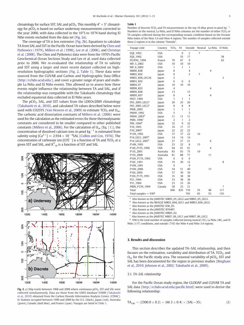
Table 1Number of discrete TCO2 and TA measurements in the top 10 dbar given in μmol kg−1.Numbers in the neutral, La Niña, and El Niño columns are the number of either TCO2 orTA samples collected during the corresponding oceanic condition based on the OceanicNiño Index of the Nino 3.4 and Nino 4 regions. The number of samples collected outsidethese 2 regions is in the column “Outside”.

Voyage code Country TCO2 TA Outside Neutral La Niña El Niño

EQF_1992 USA 9 2 7EQS_1992 USA 55 17 38FLUPAC_1994 France 70 67 9 62MP_5_2002 USA 10 10 10MP_6_2002 USA 1 1 1MR00_K08 Japan 8 4 4MR02_K02 Japan 9 2 7MR02_K06_LEG34 Japan 2 2MR03_K02 Japan 6 6 6MR04_07 Japan 10 10 10MR98_K02 Japan 4 4MR99_K06 Japan 13 13MR99_K07 Japan 8 4 4P02T_1994 USA 1 1 1P03_2005_LEG2a Japan 26 25 26P03_2005_LEG3a Japan 8 8 8P06E_2003 Japan 1 1 1P06W_1992 USA 5 5P06W_2003b Japan 11 11 11P08S_1996c Japan 2 1 2P09_1994d Japan 32 9 32P10_1993 USA 16 17 17P10_2005e Japan 22 22 22P13N_1992 USA 37 37 22 16P14_LEG1_2007f Japan 14 14 14P14_LEG2_2007f Japan 27 27 21 6P14N_1993 USA 23 22 8 15

3M. Kuchinke et al. / Marine Chemistry 161 (2014) 1–13

climatology for surface SST, SAL and pCO2. This monthly 4° × 5° climatol-ogy for pCO2 is based on surface underway measurements corrected tothe year 2000, with data collected in the 10°S to 10°N band during ElNiño events excluded from the data set (Fig. 2a).

The coverage of TA is less extensive (Fig. 2b). Equations to calculateTA from SAL and SST in the Pacific Ocean have beenderived by Chen andPytkowicz (1979), Millero et al. (1998), Lee et al. (2006), and Christianet al. (2008). The Chen and Pytkowicz data were from the 1970's PacificGeochemical Ocean Sections Study and Lee et al. used data collectedprior to 2006. We re-evaluated the relationship of TA to salinityand SST using a larger and more recent dataset collected on high-resolution hydrographic sections (Fig. 2, Table 1). These data weresourced from the CLIVAR and Carbon and Hydrographic Data Office(http://cchdo.ucsd.edu/), and cover a greater range of years and multi-ple La Niña and El Niño events. This allowed us to assess how theseevents might influence the relationship between TA and SAL, and ifthe relationship was compatible with the Takahashi climatology thatexcluded equatorial data collected in El Niño years.

The pCO2, SAL, and SST values from the LDEOv2009 climatology(Takahashi et al., 2010), and calculated TA values described below wereused with CO2SYS (Van Heuven et al., 2009) to estimate TCO2 and Ωar.The carbonic acid dissociation constants of Millero et al. (2006) wereused for the calculation as the estimated errors for these thermodynamicconstants are considered to be smaller compared to other publishedconstants (Millero et al., 2006). For the calculation of Ωar (Eq. (1)), theconcentration of dissolved calcium ions in μmol kg−1 is estimated fromsalinity using [Ca2+] = 2.934 × 10−4SAL (Culkin and Cox, 1976). Theconcentration of carbonate ion [CO3

2−] is a function of TA and TCO2 at agiven SST and SAL, and K⁎sp is a function of SST and SAL.

Fig. 2. a) Ship tracks between 1968 and 2008 where continuous pCO2, SST and SAL werecollected simultaneously. Data are those from the LDEO database V2009 (Takahashiet al., 2010) obtained from the Carbon Dioxide Information Analysis Center (CDIAC).b) Stations occupied between 1990 and 2009 by the U.S. (black), Japan (red), Australia(green), Canada (dark blue), and France (cyan). Voyages are listed in Table 1.

P14S_P15S_1996 USA 64 61 61 4P15S_2001 Australia 85 83 75 10P15S_2009 Australia 81 88 77 11P16A_P17A_1992 USA 6 6 6P16C_1991 USA 19 20 12 8P16N_1991 USA 9 9P16N_2006 USA 54 51 40 15P16S_2005 USA 37 39 39P16S_P17S_1991 USA 35 38 38P21_1994 USA 33 38 38P31_1994 USA 23 23 26PR06_P15N_1994 Canada 28 25 21 7Total 840 825 710 55 48 117Total samples = 930g 76% 6% 5% 13%

a Also known as the JAMSTEC MR05_05_LEG2 and MR05_05_LEG3.b Also known as the BEAGLE MR03_K04_LEG1 and MR03_K04_LEG2.c Also known as the JAMSTEC K96_05.d Also known as the JAMSTEC RY9407.e Also known as the JAMSTEC MR05_02.f Also known as the JAMSTEC MR07_06_LEG1 and MR07_06_LEG2.g 930 is the total number of samples collected during neutral (55), La Niña (48), and El

Niño (117) conditions, and outside (710) the Niño 4 and Niño 3.4 regions.

3. Results and discussion

This section describes the updated TA–SAL relationship, and thenfocuses on the estimation, variability and distribution of TA, TCO2, andΩar for the Pacific study area. The seasonal variability of pCO2, SST andSAL has been documented for the region in previous studies (Binghamet al., 2010; Johnson et al., 2002; Takahashi et al., 2009).

3.1. TA–SAL relationship

For the Pacific Ocean study region, the GLODAP and CLIVAR TA andSAL data (http://cchdo.ucsd.edu/pacific.html) were used to derive thefollowing relationship:

TAcalc ¼ 2300:0� 0:2ð Þ þ 66:3� 0:4ð Þ � SAL−35ð Þ: ð2Þ

4 M. Kuchinke et al. / Marine Chemistry 161 (2014) 1–13

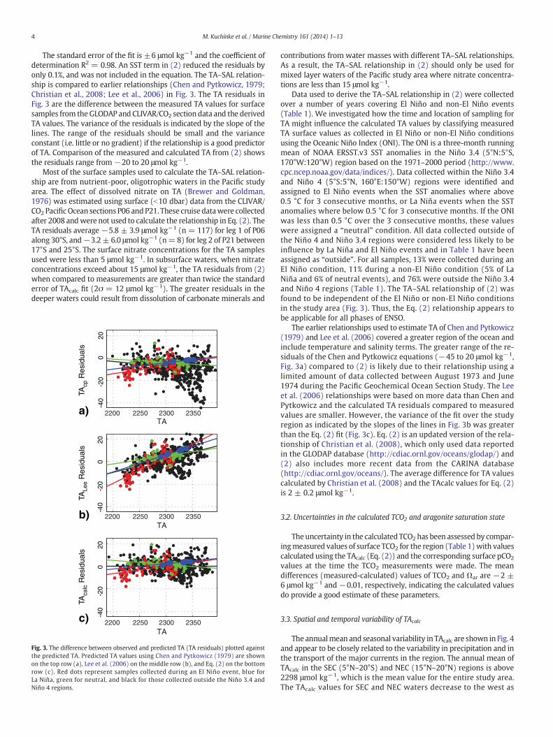
The standard error of the fit is ±6 μmol kg−1 and the coefficient ofdetermination R2 = 0.98. An SST term in (2) reduced the residuals byonly 0.1%, and was not included in the equation. The TA–SAL relation-ship is compared to earlier relationships (Chen and Pytkowicz, 1979;Christian et al., 2008; Lee et al., 2006) in Fig. 3. The TA residuals inFig. 3 are the difference between the measured TA values for surfacesamples from theGLODAP and CLIVAR/CO2 section data and the derivedTA values. The variance of the residuals is indicated by the slope of thelines. The range of the residuals should be small and the varianceconstant (i.e. little or no gradient) if the relationship is a good predictorof TA. Comparison of the measured and calculated TA from (2) showsthe residuals range from −20 to 20 μmol kg−1.

Most of the surface samples used to calculate the TA–SAL relation-ship are from nutrient-poor, oligotrophic waters in the Pacific studyarea. The effect of dissolved nitrate on TA (Brewer and Goldman,1976) was estimated using surface (b10 dbar) data from the CLIVAR/CO2 Pacific Ocean sections P06 andP21. These cruise datawere collectedafter 2008 andwere not used to calculate the relationship in Eq. (2). TheTA residuals average −5.8 ± 3.9 μmol kg−1 (n = 117) for leg 1 of P06along 30°S, and−3.2± 6.0 μmol kg−1 (n= 8) for leg 2 of P21 between17°S and 25°S. The surface nitrate concentrations for the TA samplesused were less than 5 μmol kg−1. In subsurface waters, when nitrateconcentrations exceed about 15 μmol kg−1, the TA residuals from (2)when compared to measurements are greater than twice the standarderror of TAcalc fit (2σ = 12 μmol kg−1). The greater residuals in thedeeper waters could result from dissolution of carbonate minerals and

a)

b)

c)

Fig. 3. The difference between observed and predicted TA (TA residuals) plotted againstthe predicted TA. Predicted TA values using Chen and Pytkowicz (1979) are shownon the top row (a), Lee et al. (2006) on the middle row (b), and Eq. (2) on the bottomrow (c). Red dots represent samples collected during an El Niño event, blue forLa Niña, green for neutral, and black for those collected outside the Niño 3.4 andNiño 4 regions.

contributions from water masses with different TA–SAL relationships.As a result, the TA–SAL relationship in (2) should only be used formixed layer waters of the Pacific study area where nitrate concentra-tions are less than 15 μmol kg−1.

Data used to derive the TA–SAL relationship in (2) were collectedover a number of years covering El Niño and non-El Niño events(Table 1). We investigated how the time and location of sampling forTA might influence the calculated TA values by classifying measuredTA surface values as collected in El Niño or non-El Niño conditionsusing the Oceanic Niño Index (ONI). The ONI is a three-month runningmean of NOAA ERSST.v3 SST anomalies in the Niño 3.4 (5°N:5°S,170°W:120°W) region based on the 1971–2000 period (http://www.cpc.ncep.noaa.gov/data/indices/). Data collected within the Niño 3.4and Niño 4 (5°S:5°N, 160°E:150°W) regions were identified andassigned to El Niño events when the SST anomalies where above0.5 °C for 3 consecutive months, or La Niña events when the SSTanomalies where below 0.5 °C for 3 consecutive months. If the ONIwas less than 0.5 °C over the 3 consecutive months, these valueswere assigned a “neutral” condition. All data collected outside ofthe Niño 4 and Niño 3.4 regions were considered less likely to beinfluence by La Niña and El Niño events and in Table 1 have beenassigned as “outside”. For all samples, 13% were collected during anEl Niño condition, 11% during a non-El Niño condition (5% of LaNiña and 6% of neutral events), and 76% were outside the Niño 3.4and Niño 4 regions (Table 1). The TA–SAL relationship of (2) wasfound to be independent of the El Niño or non-El Niño conditionsin the study area (Fig. 3). Thus, the Eq. (2) relationship appears tobe applicable for all phases of ENSO.

The earlier relationships used to estimate TA of Chen and Pytkowicz(1979) and Lee et al. (2006) covered a greater region of the ocean andinclude temperature and salinity terms. The greater range of the re-siduals of the Chen and Pytkowicz equations (−45 to 20 μmol kg−1,Fig. 3a) compared to (2) is likely due to their relationship using alimited amount of data collected between August 1973 and June1974 during the Pacific Geochemical Ocean Section Study. The Leeet al. (2006) relationships were based on more data than Chen andPytkowicz and the calculated TA residuals compared to measuredvalues are smaller. However, the variance of the fit over the studyregion as indicated by the slopes of the lines in Fig. 3b was greaterthan the Eq. (2) fit (Fig. 3c). Eq. (2) is an updated version of the rela-tionship of Christian et al. (2008), which only used data reportedin the GLODAP database (http://cdiac.ornl.gov/oceans/glodap/) and(2) also includes more recent data from the CARINA database(http://cdiac.ornl.gov/oceans/). The average difference for TA valuescalculated by Christian et al. (2008) and the TAcalc values for Eq. (2)is 2 ± 0.2 μmol kg−1.

3.2. Uncertainties in the calculated TCO2 and aragonite saturation state

Theuncertainty in the calculated TCO2 has been assessed by compar-ingmeasured values of surface TCO2 for the region (Table 1)with valuescalculated using the TAcalc (Eq. (2)) and the corresponding surface pCO2

values at the time the TCO2 measurements were made. The meandifferences (measured-calculated) values of TCO2 and Ωar are −2 ±6 μmol kg−1 and −0.01, respectively, indicating the calculated valuesdo provide a good estimate of these parameters.

3.3. Spatial and temporal variability of TAcalc

The annualmean and seasonal variability in TAcalc are shown in Fig. 4and appear to be closely related to the variability in precipitation and inthe transport of the major currents in the region. The annual mean ofTAcalc in the SEC (5°N–20°S) and NEC (15°N–20°N) regions is above2298 μmol kg−1, which is the mean value for the entire study area.The TAcalc values for SEC and NEC waters decrease to the west as

a) Annaul Mean TA

b) Month of min TA

c) Season Amplitude TA

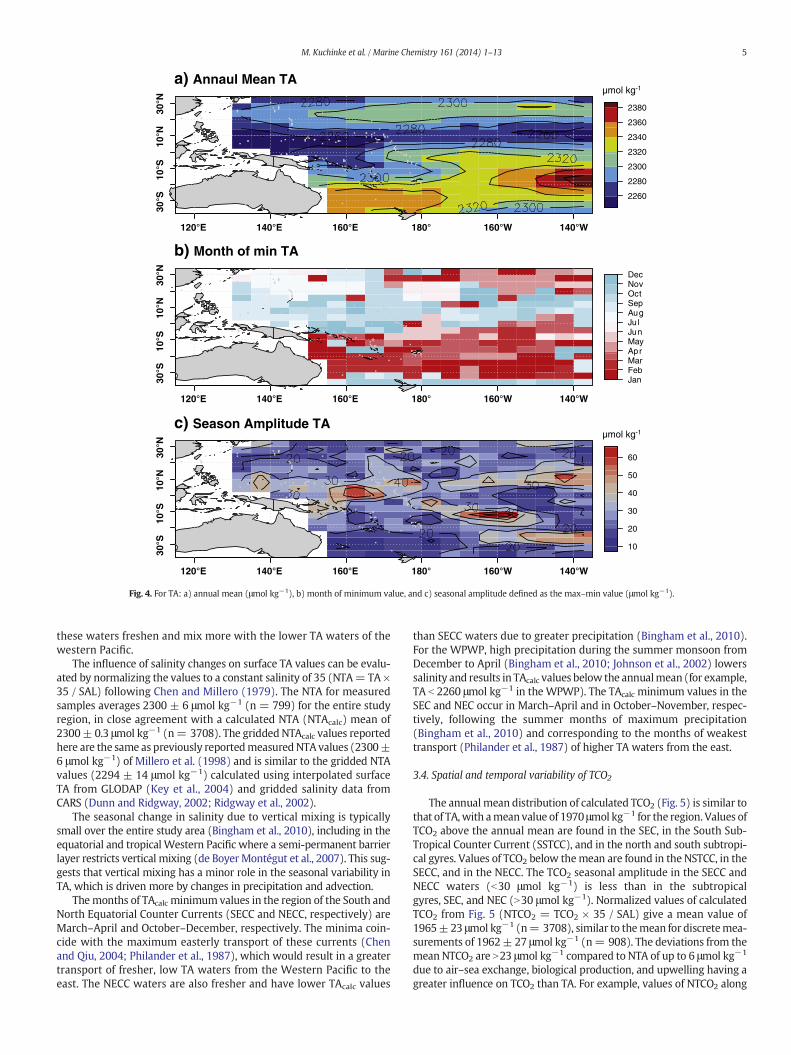
Fig. 4. For TA: a) annual mean (μmol kg−1), b) month of minimum value, and c) seasonal amplitude defined as the max–min value (μmol kg−1).

5M. Kuchinke et al. / Marine Chemistry 161 (2014) 1–13

these waters freshen and mix more with the lower TA waters of thewestern Pacific.

The influence of salinity changes on surface TA values can be evalu-ated by normalizing the values to a constant salinity of 35 (NTA= TA ×35 / SAL) following Chen and Millero (1979). The NTA for measuredsamples averages 2300 ± 6 μmol kg−1 (n = 799) for the entire studyregion, in close agreement with a calculated NTA (NTAcalc) mean of2300± 0.3 μmol kg−1 (n= 3708). The gridded NTAcalc values reportedhere are the same as previously reportedmeasuredNTA values (2300±6 μmol kg−1) of Millero et al. (1998) and is similar to the gridded NTAvalues (2294 ± 14 μmol kg−1) calculated using interpolated surfaceTA from GLODAP (Key et al., 2004) and gridded salinity data fromCARS (Dunn and Ridgway, 2002; Ridgway et al., 2002).

The seasonal change in salinity due to vertical mixing is typicallysmall over the entire study area (Bingham et al., 2010), including in theequatorial and tropical Western Pacific where a semi-permanent barrierlayer restricts vertical mixing (de Boyer Montégut et al., 2007). This sug-gests that vertical mixing has a minor role in the seasonal variability inTA, which is driven more by changes in precipitation and advection.

Themonths of TAcalc minimum values in the region of the South andNorth Equatorial Counter Currents (SECC and NECC, respectively) areMarch–April and October–December, respectively. The minima coin-cide with the maximum easterly transport of these currents (Chenand Qiu, 2004; Philander et al., 1987), which would result in a greatertransport of fresher, low TA waters from the Western Pacific to theeast. The NECC waters are also fresher and have lower TAcalc values

than SECC waters due to greater precipitation (Bingham et al., 2010).For the WPWP, high precipitation during the summer monsoon fromDecember to April (Bingham et al., 2010; Johnson et al., 2002) lowerssalinity and results in TAcalc values below the annualmean (for example,TA b 2260 μmol kg−1 in the WPWP). The TAcalc minimum values in theSEC and NEC occur in March–April and in October–November, respec-tively, following the summer months of maximum precipitation(Bingham et al., 2010) and corresponding to the months of weakesttransport (Philander et al., 1987) of higher TA waters from the east.

3.4. Spatial and temporal variability of TCO2

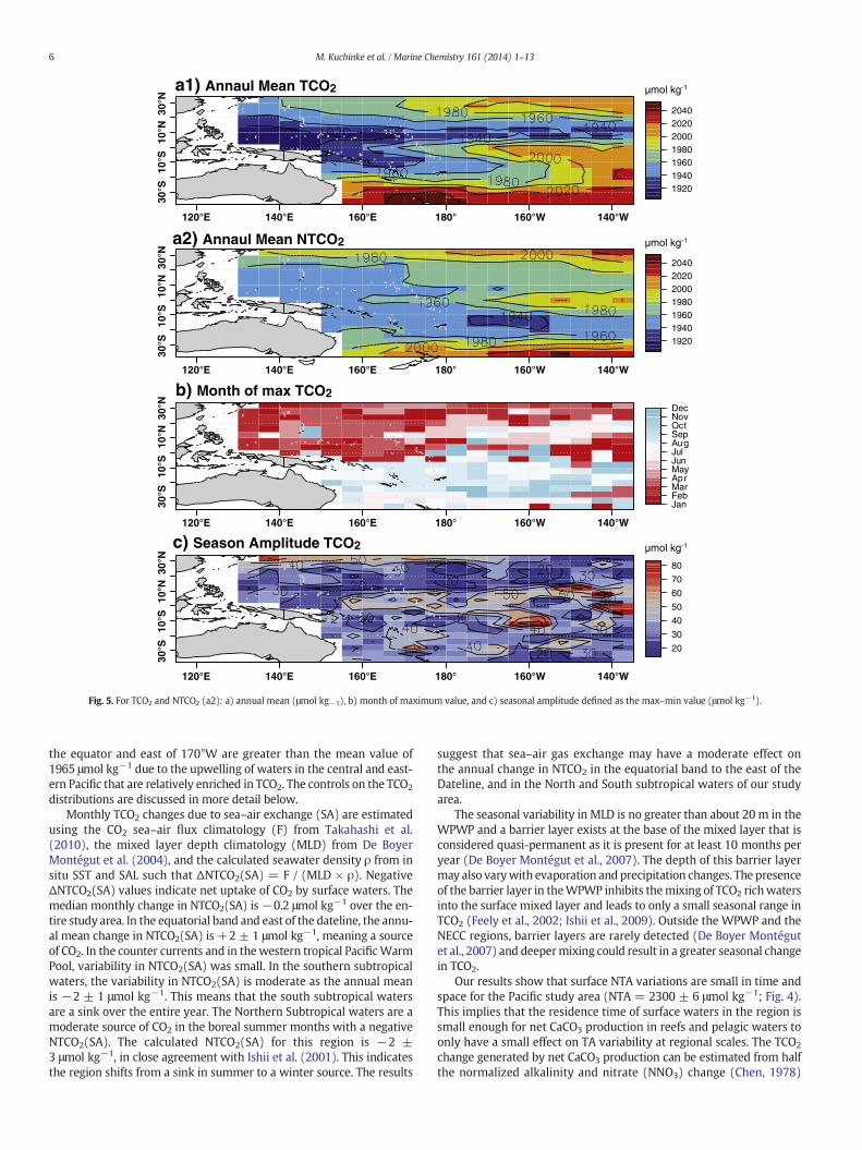
The annual mean distribution of calculated TCO2 (Fig. 5) is similar tothat of TA,with ameanvalue of 1970 μmol kg−1 for the region. Values ofTCO2 above the annual mean are found in the SEC, in the South Sub-Tropical Counter Current (SSTCC), and in the north and south subtropi-cal gyres. Values of TCO2 below themean are found in the NSTCC, in theSECC, and in the NECC. The TCO2 seasonal amplitude in the SECC andNECC waters (b30 μmol kg−1) is less than in the subtropicalgyres, SEC, and NEC (N30 μmol kg−1). Normalized values of calculatedTCO2 from Fig. 5 (NTCO2 = TCO2 × 35 / SAL) give a mean value of1965±23 μmol kg−1 (n= 3708), similar to themean for discretemea-surements of 1962± 27 μmol kg−1 (n= 908). The deviations from themean NTCO2 are N23 μmol kg−1 compared to NTA of up to 6 μmol kg−1

due to air–sea exchange, biological production, and upwelling having agreater influence on TCO2 than TA. For example, values of NTCO2 along

a1) Annaul Mean TCO2

a2) Annaul Mean NTCO2

b) Month of max TCO2

c) Season Amplitude TCO2

Fig. 5. For TCO2 and NTCO2 (a2): a) annual mean (μmol kg−1), b) month of maximum value, and c) seasonal amplitude defined as the max–min value (μmol kg−1).

6 M. Kuchinke et al. / Marine Chemistry 161 (2014) 1–13

the equator and east of 170°W are greater than the mean value of1965 μmol kg−1 due to the upwelling of waters in the central and east-ern Pacific that are relatively enriched in TCO2. The controls on the TCO2

distributions are discussed in more detail below.Monthly TCO2 changes due to sea–air exchange (SA) are estimated

using the CO2 sea–air flux climatology (F) from Takahashi et al.(2010), the mixed layer depth climatology (MLD) from De BoyerMontégut et al. (2004), and the calculated seawater density ρ from insitu SST and SAL such that ΔNTCO2(SA) = F / (MLD × ρ). NegativeΔNTCO2(SA) values indicate net uptake of CO2 by surface waters. Themedian monthly change in NTCO2(SA) is −0.2 μmol kg−1 over the en-tire study area. In the equatorial band and east of the dateline, the annu-al mean change in NTCO2(SA) is +2 ± 1 μmol kg−1, meaning a sourceof CO2. In the counter currents and in thewestern tropical PacificWarmPool, variability in NTCO2(SA) was small. In the southern subtropicalwaters, the variability in NTCO2(SA) is moderate as the annual meanis −2 ± 1 μmol kg−1. This means that the south subtropical watersare a sink over the entire year. The Northern Subtropical waters are amoderate source of CO2 in the boreal summer months with a negativeNTCO2(SA). The calculated NTCO2(SA) for this region is −2 ±3 μmol kg−1, in close agreement with Ishii et al. (2001). This indicatesthe region shifts from a sink in summer to a winter source. The results

suggest that sea–air gas exchange may have a moderate effect onthe annual change in NTCO2 in the equatorial band to the east of theDateline, and in the North and South subtropical waters of our studyarea.

The seasonal variability in MLD is no greater than about 20 m in theWPWP and a barrier layer exists at the base of the mixed layer that isconsidered quasi-permanent as it is present for at least 10 months peryear (De Boyer Montégut et al., 2007). The depth of this barrier layermay also varywith evaporation and precipitation changes. The presenceof the barrier layer in theWPWP inhibits themixing of TCO2 richwatersinto the surface mixed layer and leads to only a small seasonal range inTCO2 (Feely et al., 2002; Ishii et al., 2009). Outside the WPWP and theNECC regions, barrier layers are rarely detected (De Boyer Montégutet al., 2007) and deepermixing could result in a greater seasonal changein TCO2.

Our results show that surface NTA variations are small in time andspace for the Pacific study area (NTA = 2300 ± 6 μmol kg−1; Fig. 4).This implies that the residence time of surface waters in the region issmall enough for net CaCO3 production in reefs and pelagic waters toonly have a small effect on TA variability at regional scales. The TCO2

change generated by net CaCO3 production can be estimated from halfthe normalized alkalinity and nitrate (NNO3) change (Chen, 1978)

7M. Kuchinke et al. / Marine Chemistry 161 (2014) 1–13

such that ΔNTCO2(CaCO3) = −0.5 × (ΔNTA + ΔNNO3). The annualmean NO3 concentration along the equator increases eastward from 1to 5 μmol kg−1 and the rest of the region has an annual mean of0.25 μmol kg−1 (Garcia et al., 2010). Hence, the annual maximumestimated ΔNTCO2(CaCO3) is 2.5 μmol kg−1. Based on this analysis,net calcification does not appear to have a significant impact on thelarge seasonal or regional changes in TCO2. However, localized calcifica-tion and production could influence TCO2 and TA variability at the scaleof coral reefs (Shaw et al., 2012).

3.5. Spatial and temporal variability of Ωar in the tropical Pacific

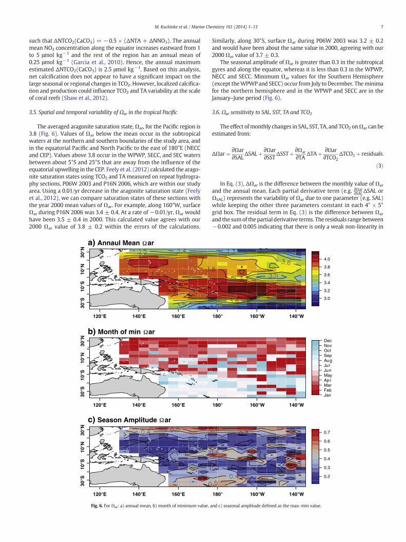
The averaged aragonite saturation state,Ωar, for the Pacific region is3.8 (Fig. 6). Values of Ωar below the mean occur in the subtropicalwaters at the northern and southern boundaries of the study area, andin the equatorial Pacific and North Pacific to the east of 180°E (NECCand CEP). Values above 3.8 occur in the WPWP, SECC, and SEC watersbetween about 5°S and 25°S that are away from the influence of theequatorial upwelling in the CEP. Feely et al. (2012) calculated the arago-nite saturation states using TCO2 and TAmeasured on repeat hydrogra-phy sections, P06W 2003 and P16N 2006, which are within our studyarea. Using a 0.01/yr decrease in the aragonite saturation state (Feelyet al., 2012), we can compare saturation states of these sections withthe year 2000 mean values of Ωar. For example, along 160°W, surfaceΩar during P16N 2006 was 3.4 ± 0.4. At a rate of −0.01/yr, Ωar wouldhave been 3.5 ± 0.4 in 2000. This calculated value agrees with our2000 Ωar value of 3.8 ± 0.2 within the errors of the calculations.

c) Season Amplitude ar

b) Month of min ar

a) Annaul Mean ar

Fig. 6. For Ωar: a) annual mean, b) month of minimum value, a

Similarly, along 30°S, surface Ωar during P06W 2003 was 3.2 ± 0.2and would have been about the same value in 2000, agreeing with our2000 Ωar value of 3.7 ± 0.3.

The seasonal amplitude of Ωar is greater than 0.3 in the subtropicalgyres and along the equator, whereas it is less than 0.3 in the WPWP,NECC and SECC. Minimum Ωar values for the Southern Hemisphere(except theWPWP and SECC) occur from July to December. Theminimafor the northern hemisphere and in the WPWP and SECC are in theJanuary–June period (Fig. 6).

3.6. Ωar sensitivity to SAL, SST, TA and TCO2

The effect ofmonthly changes in SAL, SST, TA, and TCO2 onΩar can beestimated from:

ΔΩar ¼ ∂Ωar∂SALΔSAL þ

∂Ωar∂SST ΔSSTþ ∂Ωar

∂TA ΔTAþ ∂Ωar∂TCO2

ΔTCO2 þ residuals:

ð3Þ

In Eq. (3), ΔΩar is the difference between the monthly value of Ωar

and the annual mean. Each partial derivative term (e.g. ∂Ωar∂SALΔSAL or

ΩSAL) represents the variability of Ωar due to one parameter (e.g. SAL)while keeping the other three parameters constant in each 4° × 5°grid box. The residual term in Eq. (3) is the difference between Ωar

and the sumof thepartial derivative terms. The residuals range between−0.002 and 0.005 indicating that there is only a weak non-linearity in

nd c) seasonal amplitude defined as the max–min value.

a) Season Amplitude SST b) Month of min SST

c) Season Amplitude TA d) Month of min TA

e) Season Amplitude TCO2 f) Month of min TCO2

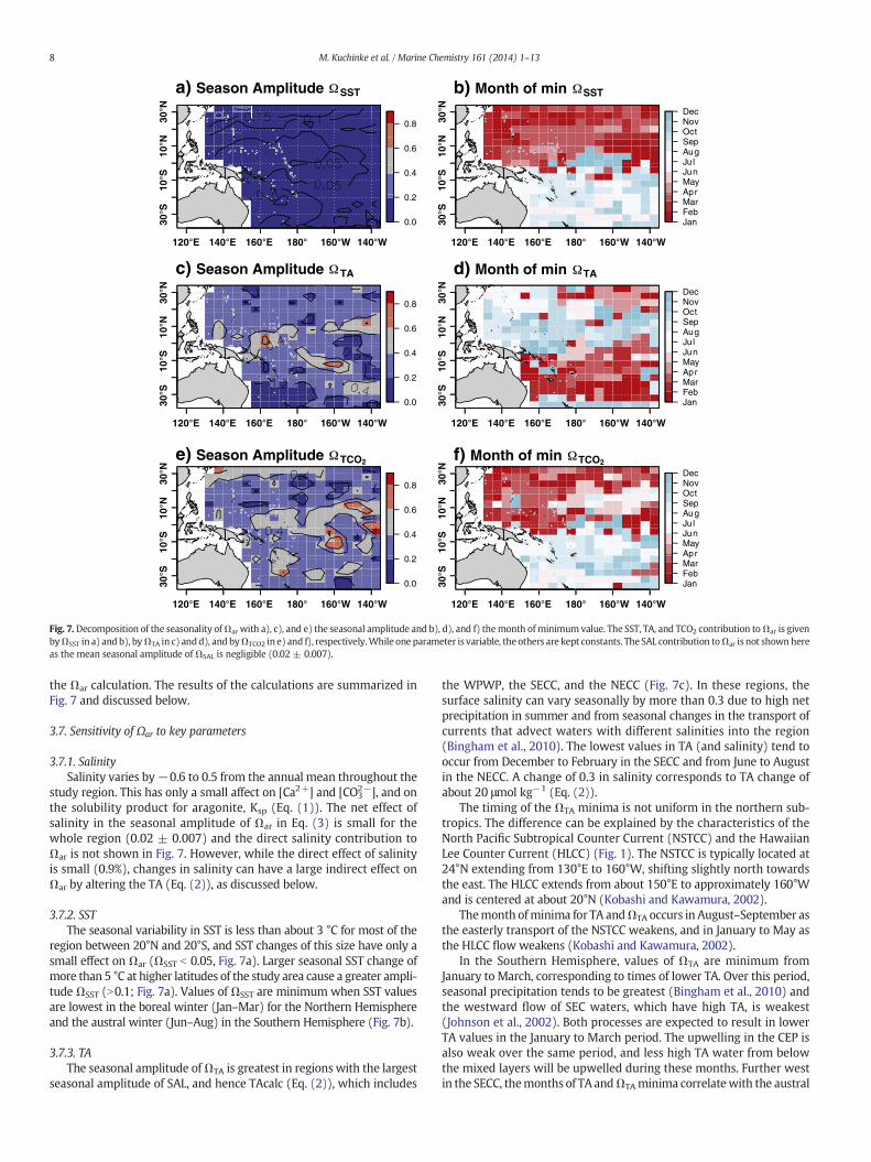
Fig. 7.Decomposition of the seasonality ofΩar with a), c), and e) the seasonal amplitude and b), d), and f) themonth ofminimum value. The SST, TA, and TCO2 contribution toΩar is givenbyΩSST in a) and b), byΩTA in c) andd), and byΩTCO2 in e) and f), respectively.While one parameter is variable, the others are kept constants. The SAL contribution toΩar is not shownhereas the mean seasonal amplitude of ΩSAL is negligible (0.02 ± 0.007).

8 M. Kuchinke et al. / Marine Chemistry 161 (2014) 1–13

the Ωar calculation. The results of the calculations are summarized inFig. 7 and discussed below.

3.7. Sensitivity of Ωar to key parameters

3.7.1. SalinitySalinity varies by−0.6 to 0.5 from the annual mean throughout the

study region. This has only a small affect on [Ca2+] and [CO32−], and on

the solubility product for aragonite, Ksp (Eq. (1)). The net effect ofsalinity in the seasonal amplitude of Ωar in Eq. (3) is small for thewhole region (0.02 ± 0.007) and the direct salinity contribution toΩar is not shown in Fig. 7. However, while the direct effect of salinityis small (0.9%), changes in salinity can have a large indirect effect onΩar by altering the TA (Eq. (2)), as discussed below.

3.7.2. SSTThe seasonal variability in SST is less than about 3 °C for most of the

region between 20°N and 20°S, and SST changes of this size have only asmall effect on Ωar (ΩSST b 0.05, Fig. 7a). Larger seasonal SST change ofmore than 5 °C at higher latitudes of the study area cause a greater ampli-tude ΩSST (N0.1; Fig. 7a). Values of ΩSST are minimum when SST valuesare lowest in the boreal winter (Jan–Mar) for the Northern Hemisphereand the austral winter (Jun–Aug) in the Southern Hemisphere (Fig. 7b).

3.7.3. TAThe seasonal amplitude ofΩTA is greatest in regions with the largest

seasonal amplitude of SAL, and hence TAcalc (Eq. (2)), which includes

the WPWP, the SECC, and the NECC (Fig. 7c). In these regions, thesurface salinity can vary seasonally by more than 0.3 due to high netprecipitation in summer and from seasonal changes in the transport ofcurrents that advect waters with different salinities into the region(Bingham et al., 2010). The lowest values in TA (and salinity) tend tooccur from December to February in the SECC and from June to Augustin the NECC. A change of 0.3 in salinity corresponds to TA change ofabout 20 μmol kg−1 (Eq. (2)).

The timing of the ΩTA minima is not uniform in the northern sub-tropics. The difference can be explained by the characteristics of theNorth Pacific Subtropical Counter Current (NSTCC) and the HawaiianLee Counter Current (HLCC) (Fig. 1). The NSTCC is typically located at24°N extending from 130°E to 160°W, shifting slightly north towardsthe east. The HLCC extends from about 150°E to approximately 160°Wand is centered at about 20°N (Kobashi and Kawamura, 2002).

Themonth ofminima for TA andΩTA occurs in August–September asthe easterly transport of the NSTCC weakens, and in January to May asthe HLCC flow weakens (Kobashi and Kawamura, 2002).

In the Southern Hemisphere, values of ΩTA are minimum fromJanuary to March, corresponding to times of lower TA. Over this period,seasonal precipitation tends to be greatest (Bingham et al., 2010) andthe westward flow of SEC waters, which have high TA, is weakest(Johnson et al., 2002). Both processes are expected to result in lowerTA values in the January to March period. The upwelling in the CEP isalso weak over the same period, and less high TA water from belowthe mixed layers will be upwelled during these months. Further westin the SECC, themonths of TA andΩTAminima correlatewith the austral

9M. Kuchinke et al. / Marine Chemistry 161 (2014) 1–13

summer (December–February) when high precipitation (Brown et al.,2010) will lower surface salinity and TA (Eq. (2)).

3.7.4. TCO2

As shown in the following sections, TCO2 is a major driver in Ωar

variability throughout the region. The ΩTCO2 values are low in wintermonthswhen surface TCO2 is higher due to deepermixed layers, poten-tially greater net respiration in some regions (Ishii et al., 2001) or lowernet primary production (Behrenfeld et al., 2005), and possibly theadvection of CO2 rich waters into a region. Values of ΩTCO2 vary bymore than 0.3 in the equatorial zone and in the subtropical gyreswhere the seasonal variability of TCO2 is greater than 20 μmol kg−1.For the remainder of the study area, seasonal changes of less than20 μmol kg−1 occur in TCO2 in the WPWP, SECC and NECC and resultin seasonal changes of less than 0.3ΩTCO2. These are regions of relativelylow wind and high precipitation that contribute to low salinity surfaceand a thickening of the barrier layer, inhibiting the exchange of CO2

between the deep and surface oceans (Ishii et al., 2001).We now describe and discuss the relative contribution of TCO2,

TA, SST and SAL changes to the seasonal Ωar variability in the Pacificsub-regions of 1) WPWP and NECC, 2) the CEP, and 3) the SEC. Thissensitivity analysis uses Eq. (3) with plots for each subregion shownin Figs. 8–11. The variabilities of TCO2 and TA, and SST and SAL arepaired for scaling convenience and shown in the top and middle panelsrespectively. These are calculated as the deviation of the monthlyaverage values from the annual mean of each parameter. The sensi-tivity of Ωar to the respective parameter variability is shown in thebottom panel.

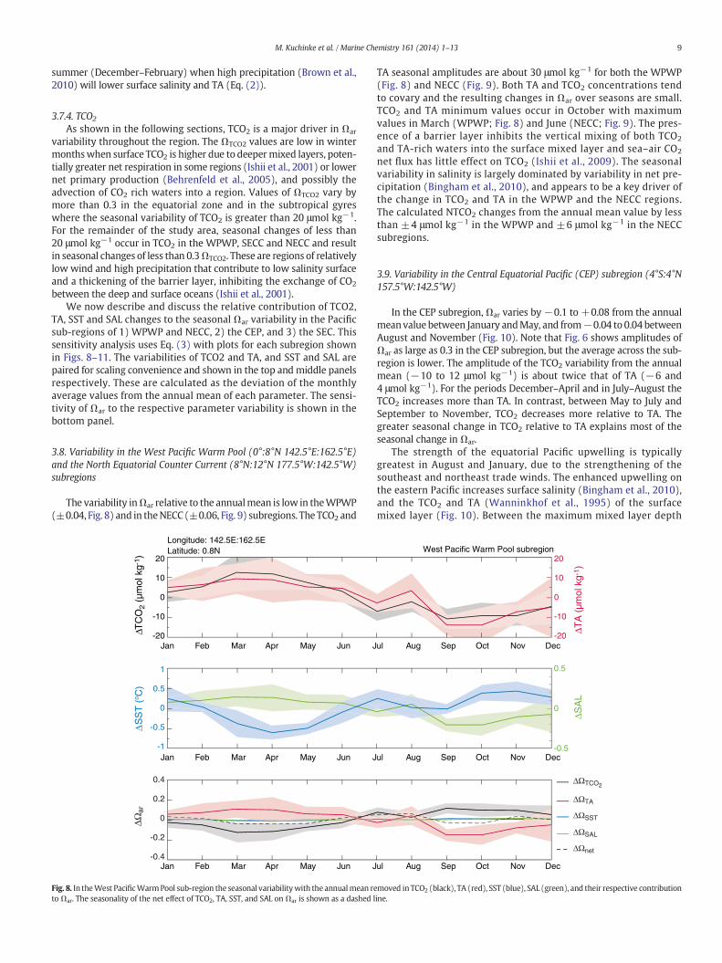
3.8. Variability in the West Pacific Warm Pool (0°:8°N 142.5°E:162.5°E)and the North Equatorial Counter Current (8°N:12°N 177.5°W:142.5°W)subregions

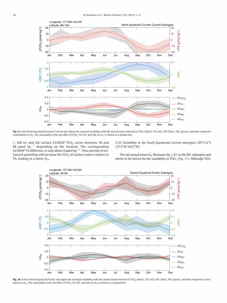
The variability inΩar relative to the annualmean is low in theWPWP(±0.04, Fig. 8) and in theNECC (±0.06, Fig. 9) subregions. The TCO2 and

Longitude: 142.5E:162.5ELatitude: 0.8N

Jan Feb Mar Apr May Jun J

Jan Feb Mar Apr May Jun J

Jan Feb Mar Apr May Jun J

20

10

0

-10

-20

1

0.5

0

-0.5

-1

ΔTC

O2

(µm

ol k

g-1 )

ΔS

ST

(o C

)

0.4

0.2

0

-0.2

-0.4

ΔΩar

Fig. 8. In theWest PacificWarmPool sub-region the seasonal variabilitywith the annualmean reto Ωar. The seasonality of the net effect of TCO2, TA, SST, and SAL on Ωar is shown as a dashed l

TA seasonal amplitudes are about 30 μmol kg−1 for both the WPWP(Fig. 8) and NECC (Fig. 9). Both TA and TCO2 concentrations tendto covary and the resulting changes in Ωar over seasons are small.TCO2 and TA minimum values occur in October with maximumvalues in March (WPWP; Fig. 8) and June (NECC; Fig. 9). The pres-ence of a barrier layer inhibits the vertical mixing of both TCO2

and TA-rich waters into the surface mixed layer and sea–air CO2

net flux has little effect on TCO2 (Ishii et al., 2009). The seasonalvariability in salinity is largely dominated by variability in net pre-cipitation (Bingham et al., 2010), and appears to be a key driver ofthe change in TCO2 and TA in the WPWP and the NECC regions.The calculated NTCO2 changes from the annual mean value by lessthan ±4 μmol kg−1 in the WPWP and ±6 μmol kg−1 in the NECCsubregions.

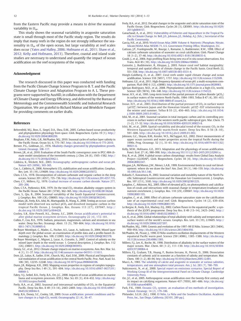
3.9. Variability in the Central Equatorial Pacific (CEP) subregion (4°S:4°N157.5°W:142.5°W)

In the CEP subregion, Ωar varies by −0.1 to +0.08 from the annualmeanvalue between January andMay, and from−0.04 to 0.04 betweenAugust and November (Fig. 10). Note that Fig. 6 shows amplitudes ofΩar as large as 0.3 in the CEP subregion, but the average across the sub-region is lower. The amplitude of the TCO2 variability from the annualmean (−10 to 12 μmol kg−1) is about twice that of TA (−6 and4 μmol kg−1). For the periods December–April and in July–August theTCO2 increases more than TA. In contrast, between May to July andSeptember to November, TCO2 decreases more relative to TA. Thegreater seasonal change in TCO2 relative to TA explains most of theseasonal change in Ωar.

The strength of the equatorial Pacific upwelling is typicallygreatest in August and January, due to the strengthening of thesoutheast and northeast trade winds. The enhanced upwelling onthe eastern Pacific increases surface salinity (Bingham et al., 2010),and the TCO2 and TA (Wanninkhof et al., 1995) of the surfacemixed layer (Fig. 10). Between the maximum mixed layer depth

West Pacific Warm Pool subregion

ul Aug Sep Oct Nov Dec

ul Aug Sep Oct Nov Dec

ul Aug Sep Oct Nov Dec

20

10

0

-10

-20

0.5

0

-0.5

ΔSA

LΔT

A (

µmol

kg-

1 )

ΔΩTCO2

ΔΩTA

ΔΩSST

ΔΩSAL

ΔΩnet

moved in TCO2 (black), TA (red), SST (blue), SAL (green), and their respective contributionine.

Longitude: 177.5W:142.5WLatitude: 8N:12N North equatorial Counter Current Subregion

Jan Feb Mar Apr May Jun Jul Aug Sep Oct Nov Dec

Jan Feb Mar Apr May Jun Jul Aug Sep Oct Nov Dec

Jan Feb Mar Apr May Jun Jul Aug Sep Oct Nov Dec

20

10

0

-10

-20

1

0.5

0

-0.5

-1

20

10

0

-10

-20ΔTC

O2

(µm

ol k

g-1 )

ΔS

ST

(o C

)

0.5

0

-0.5

ΔSA

LΔT

A (

µmol

kg-

1)

0.4

0.2

0

-0.2

-0.4

ΔΩar

ΔΩTCO2

ΔΩTA

ΔΩSST

ΔΩSAL

ΔΩnet

Fig. 9. In the North Equatorial Counter Current sub-region the seasonal variability with the annual mean removed in TCO2 (black), TA (red), SST (blue), SAL (green), and their respectivecontribution toΩar. The seasonality of the net effect of TCO2, TA, SST, and SAL on Ωar is shown as a dashed line.

10 M. Kuchinke et al. / Marine Chemistry 161 (2014) 1–13

(~100 m) and the surface GLODAP TCO2 varies between 30 and68 μmol kg−1 depending on the location. The correspondingGLODAP TA difference is only about 9 μmol kg−1. Thus periods of en-hanced upwelling will increase the TCO2 of surface waters relative toTA, leading to a lower Ωar.

Longitude: 157.5W:142.5WLatitude: 4S:4N

Jan Feb Mar Apr May Jun J

Jan Feb Mar Apr May Jun J

Jan Feb Mar Apr May Jun J

20

10

0

-10

-20

1

0.5

0

-0.5

-1

ΔTC

O2

(µm

ol k

g-1

)Δ

SS

T (

o C)

0.4

0.2

0

-0.2

-0.4

ΔΩar

Fig. 10. In the Central Equatorial Pacific sub-region the seasonal variability with the annual mebution toΩar. The seasonality of the net effect of TCO2, TA, SST, and SAL on Ωar is shown as a d

3.10. Variability in the South Equatorial Current subregion (20°S:12°S157.5°W:142.5°W)

The net annualmeanΩar fluctuates by±0.1 in the SEC subregion andseems to be driven by the variability in TCO2 (Fig. 11). Although TCO2

Central Equatorial Pacific Subregion

ul Aug Sep Oct Nov Dec

ul Aug Sep Oct Nov Dec

ul Aug Sep Oct Nov Dec

20

10

0

-10

-20

0.5

0.1

-0.1

0

-0.5

ΔSA

LΔT

A (

µmol

kg-

1 )

ΔΩTCO2

ΔΩTA

ΔΩSST

ΔΩSAL

ΔΩnet

an removed in TCO2 (black), TA (red), SST (blue), SAL (green), and their respective contri-ashed line.

Longitude: 157.5W:142.5WLatitude: 20S:12S South Equatorial Current subregion

Jan Feb Mar Apr May Jun Jul Aug Sep Oct Nov Dec

Jan Feb Mar Apr May Jun Jul Aug Sep Oct Nov Dec

Jan Feb Mar Apr May Jun Jul Aug Sep Oct Nov Dec

20

10

0

-10

-20

1

0.5

0

-0.5

-1

20

10

0

-10

-20

ΔTC

O2

(µm

ol k

g-1 )

ΔSS

T (

o C)

0.2

0.1

0

-0.1

-0.2

ΔSA

LΔT

A (

µmol

kg-

1 )

0.4

0.2

0

-0.2

-0.4

ΔΩar

ΔΩTCO2

ΔΩTA

ΔΩSST

ΔΩSAL

ΔΩnet

Fig. 11. In the South Equatorial Current sub-region the seasonal variability with the annual mean removed in TCO2 (black), TA (red), SST (blue), SAL (green), and their respective contri-bution toΩar. The seasonality of the net effect of TCO2, TA, SST, and SAL on Ωar is shown as a dashed line.

11M. Kuchinke et al. / Marine Chemistry 161 (2014) 1–13

and TA vary in the same way, TCO2 decreases more than TA betweenMarch and July and increases more than TA between August andFebruary. The decoupling of TCO2 from TA results in an increaseof Ωar between March and July, and a decrease between Augustand February.

The outgassing of CO2 and vertical mixing are unlikely to cause thedifferent changes in TCO2 and TA for this region. The net sea–air fluxof CO2 in this region is close to zero (Takahashi et al., 2009). Verticalmixing or entrainment of waters has been shown to have a limited ef-fect on the seasonal variability in salinity (Binghamet al., 2010). Verticalmixing or entrainment is also unlikely to havemuch of an impact on theseasonal variability in nitrate, which could drive some changes in TCO2

relative to TA. These waters are oligotrophic (Behrenfeld et al., 2005)and seasonal changes in the biological drawdown of CO2 are also ex-pected to be low. Nitrate concentrations vary between 0.15 μmol kg−1

in the January to May period and 0.6 μmol kg−1 in the June–December(Garcia et al., 2010). Therefore the seasonal nitrate changes wouldonly produce a decrease of 1 μmol kg−1 of TCO2 in January–May and4 μmol kg−1 in June–December, using the Redfield ratio. This wouldbe less than 10% of the change calculated in TCO2. Thus, we do not ex-pect seasonal changes in biologically drawn down of CO2, sea–air gasexchange, or vertical entrainment alone could explain the decouplingof the TCO2 and TA signals.

Transport and evaporation seem to account for much of the var-iability in TCO2 and TA in the SEC subregion (Fig. 11). The variabil-ities in TCO2 and TA are coupled, and peak when the southeasttrade winds are strongest in August, enhancing net evaporation(Bingham et al., 2010) and the westward flow of the SEC(Reverdin et al., 1994), both of which would increase SAL, TCO2

and TA. The change in salinity through evaporation affects bothTCO2 and TA the same way and NTA is constant over time andspace. The TCO2/TA ratio in surface waters is greater in the easternPacific and greater transport of waters from the east from August toFebruary could cause a net decrease in Ωar. This suggests that

seasonal changes in the zonal transport of the SEC waters could ac-count for a significant component of the seasonal change in Ωar.

4. Conclusion

The goal of this study was to investigate the variability in the arago-nite saturation state (Ωar) at seasonal and basin scales for the WesternPacific (120°E:140°W and 35°S:30°N). We developed a new relation-ship between measured values of total alkalinity and salinity (Eq. (2))to provide one of the key CO2 system parameters needed to reconstructand quantify the seasonal cycle of the aragonite saturation state. TheTA–SAL relationship was found to be valid under all ENSO conditionsand applicable across the entire study region. This relationship is animprovement of previous studies and provides a way to estimatehigh-resolution surface TA fields with salinity data from observationalprograms like ARGO (Gould et al., 2004). This updated relationshipand the seasonal climatology of surface pCO2 were used to calculateTCO2 and Ωar.

The seasonal variability in Ωar is small in the Western Pacific WarmPool and the North Equatorial Counter Current subregions because TAchanges tend to offset the effect of TCO2. Net precipitation changes inthese two subregions drive the seasonal variabilities in TA and TCO2.Vertical mixing is inhibited by the quasi-permanence of a barrier layerand the sea–air exchange of CO2 and biological production were foundto have only a small influence on the Ωar variability in the WPWP andNECC subregions. The variability inΩar is larger in the Central EquatorialPacific where the seasonal upwelling of waters with a higher TCO2/TAratio than the surfacewaters causes decreases inΩar. In the South Equa-torial Current subregion, the seasonal variability inΩar is also driven bygreater changes in TCO2 relative to TA. Seasonal shifts in net biologicalproduction and verticalmixing did not appear to drive theΩar seasonal-ity for the SEC. Net evaporation changes did alter TCO2 and TA, but thechanges in both parameters were similar with little influence on Ωar.

Here, changes in the transport of waters higher in TCO2 relative to TA

12 M. Kuchinke et al. / Marine Chemistry 161 (2014) 1–13

from the Eastern Pacific may provide a means to drive the seasonalvariability in Ωar.

This study shows the seasonal variability in aragonite saturationstate is small through most of the Pacific study region. The results doimply that many reefs in the region do not strongly influence the sea-sonality in Ωar of the open ocean, but large variability at reef scalesdoes occur (Yates and Halley, 2006; Hofmann et al., 2011; Shaw et al.,2012; Kelly and Hofmann, 2013). Therefore, coastal and island scalestudies are necessary to understand and quantify the impact of oceanacidification on the reef ecosystems of the region.

Acknowledgment

The research discussed in this paper was conducted with fundingfrom the Pacific Climate Change Science Program to B. T. and the PacificClimate Change Science and Adaptation Program to A. L. These pro-gramswere supported by AusAID, in collaborationwith theDepartmentof Climate Change and Energy Efficiency, and delivered by the Bureau ofMeteorology and the Commonwealth Scientific and Industrial ResearchOrganisation. We are grateful to Richard Matear and Bénédicte Pasquerfor providing comments on earlier drafts.

References

Behrenfeld, M.J., Boss, E., Siegel, D.A., Shea, D.M., 2005. Carbon-based ocean productivityand phytoplankton physiology from space. Glob. Biogeochem. Cycles 19 (1). http://dx.doi.org/10.1029/2004GB00299.

Bingham, F.M., Foltz, G.R., McPhaden,M.J., 2010. Seasonal cycles of surface layer salinity inthe Pacific Ocean. Ocean Sci. 6, 775–787. http://dx.doi.org/10.5194/os-6-775-2010.

Brewer, P.G., Goldman, J.C., 1976. Alkalinity changes generated by phytoplankton growth.Limnol. Oceanogr. 108–117.

Brown, J.R., et al., 2010. Evaluation of the South Pacific convergence zone in IPCC AR4 cli-mate model simulations of the twentieth century. J. Clim. 24 (6), 1565–1582. http://dx.doi.org/10.1175/2010jcli3942.1.

Caldeira, K., Wickett, M.E., 2003. Oceanography: anthropogenic carbon and ocean pH.Nature 425 (6956), 365-365.

Cao, L., Caldeira, K., 2008. Atmospheric CO2 stabilization and ocean acidification. Geophys.Res. Lett. 35 (19), L19609. http://dx.doi.org/10.1029/2008GL035072.

Chen, C.T.A., 1978. Decomposition of calcium carbonate and organic carbon in the deepoceans. Science 201 (4357), 735–736. http://dx.doi.org/10.1126/science.201.4357.735.

Chen, C.T., Millero, F.J., 1979. Gradual increase of oceanic carbon dioxide. Nature 277,205–206.

Chen, C.T.A., Pytkowicz, R.M., 1979. On the total CO2–titration alkalinity–oxygen system inthe Pacific Ocean. Nature 281 (5730), 362–365. http://dx.doi.org/10.1038/281362a0.

Chen, S., Qiu, B., 2004. Seasonal variability of the South Equatorial Countercurrent.J. Geophys. Res. 109 (C8), C08003. http://dx.doi.org/10.1029/2003JC002243.

Christian, J.R., Feely, R.A., Ishii, M., Murtugudde, R.,Wang, X., 2008. Testing an ocean carbonmodel with observed sea surface pCO2 and dissolved inorganic carbon in thetropical Pacific Ocean. J. Geophys. Res. Oceans 113 (C7), C07047. http://dx.doi.org/10.1029/2007jc004428.

Cooley, S.R., Kite-Powell, H.L., Doney, S.C., 2009. Ocean acidification's potential toalter global marine ecosystem services. Oceanography 22 (4), 172–181.

Culkin, F., Cox, R.A., 1976. Sodium, potassium, magnesium, calcium and strontium in seawater. Deep Sea Res. Oceanogr. Abstr. 13 (5), 789–804. http://dx.doi.org/10.1016/0011-7471(76)90905-0.

De Boyer Montégut, C., Madec, G., Fischer, A.S., Lazar, A., Iudicone, D., 2004. Mixed layerdepth over the global ocean: an examination of profile data and a profile-based cli-matology. J. Geophys. Res. 109, C12003. http://dx.doi.org/10.1029/2004JC002378.

De Boyer Montégut, C., Mignot, J., Lazar, A., Cravatte, S., 2007. Control of salinity on themixed layer depth in the world ocean: 1. General description. J. Geophys. Res. 112(C6), C06011. http://dx.doi.org/10.1029/2006JC003953.

Doney, S.C., et al., 2012. Climate change impacts onmarine ecosystems. Ann. Rev. Mar. Sci.4 (1), 11–37. http://dx.doi.org/10.1146/annurev-marine-041911-111611.

Dore, J.E., Lukas, R., Sadler, D.W., Church, M.J., Karl, D.M., 2009. Physical and biogeochem-icalmodulation of ocean acidification in the central North Pacific. Proc. Natl. Acad. Sci.106 (30), 12235–12240. http://dx.doi.org/10.1073/pnas.0906044106.

Dunn, J.R., Ridgway, K.R., 2002. Mapping ocean properties in regions of complex topogra-phy. Deep Sea Res. I 49 (3), 591–604. http://dx.doi.org/10.1016/s0967-0637(01)00069-3.

Fabry, V.J., Seibel, B.A., Feely, R.A., Orr, J.C., 2008. Impacts of ocean acidification on marinefauna and ecosystem processes. ICES J. Mar. Sci. 65 (3), 414–432. http://dx.doi.org/10.1093/icesjms/fsn048.

Feely, R.A., et al., 2002. Seasonal and interannual variability of CO2 in the EquatorialPacific. Deep Sea Res. II 49 (13–14), 2443–2469. http://dx.doi.org/10.1016/s0967-0645(02)00044-9.

Feely, R.A., Doney, S.C., Cooley, S.R., 2009. Ocean acidification: present conditions and fu-ture changes in a high-CO2 world. Oceanography 22 (4), 36–47.

Feely, R.A., et al., 2012. Decadal changes in the aragonite and calcite saturation state of thePacific Ocean. Glob. Biogeochem. Cycles 26 (3), GB3001. http://dx.doi.org/10.1029/2011gb004157.

Ganachaud, A., et al., 2012. Vulnerability of Fisheries and Aquaculture in the Tropical Pa-cific to Climate Change. In: Bell, J.D., Johnson, J.E., Hobday, A.J. (Eds.), Secretariat of thePacific Community.

Garcia, H.E., et al., 2010. World Ocean Atlas 2009. Volume 4: Nutrients (Phosphate, Nitrate,Silicate)NOAA Atlas NESDIS 71, U.S. Government Printing Office, Washington, D.C.

Gattuso, J.P., Frankignoulle, M., Bourge, I., Romaine, S., Buddemeier, R.W., 1998. Effect ofcalcium carbonate saturation of seawater on coral calcification. Glob. Planet Change18 (1–2), 37–46. http://dx.doi.org/10.1016/s0921-8181(98)00035-6.

Gould, J., et al., 2004. Argo profiling floats bring new era of in situ ocean observations. EosTrans. AGU 85 (19). http://dx.doi.org/10.1029/2004eo190002.

Guinotte, J., Buddemeier, R., Kleypas, J., 2003. Future coral reef habitat marginality:temporal and spatial effects of climate change in the Pacific basin. Coral Reefs 22,551–558. http://dx.doi.org/10.1007/s00338-003-0331-4.

Hoegh-Guldberg, O., et al., 2007. Coral reefs under rapid climate change and oceanacidification. Science 318 (5857), 1737. http://dx.doi.org/10.1126/science.1152509.

Hofmann, G.E., et al., 2011. High-frequency dynamics of ocean pH: amulti-ecosystem com-parison. PLoS ONE 6 (12), e28983. http://dx.doi.org/10.1371/journal.pone.0028983.

Iglesias-Rodriguez, M.D., et al., 2008. Phytoplankton calcification in a high-CO2 world.Science 320 (5874), 336–340. http://dx.doi.org/10.1126/science.1154122.

Inoue, H.Y., et al., 1995. Long-term trend of the partial pressure of carbon dioxide (pCO2)in surface waters of the western North Pacific, 1984–1993. Tellus B 47 (4), 391–413.http://dx.doi.org/10.1034/j.1600-0889.47.issue4.2.x.

Inoue, H.Y., et al., 2003. Distribution of the partial pressure of CO2 in surface water(pCO2

w) between Japan and the Hawaiian Islands: pCO2w–SST relationship in

the winter and summer. Tellus B 55 (2), 456–465. http://dx.doi.org/10.1034/j.1600-0889.2003.01482.x.

Ishii, M., et al., 2001. Seasonal variation in total inorganic carbon and its controlling pro-cesses in surface waters of the western north pacific subtropical gyre. Mar. Chem. 75(1–2), 17–32. http://dx.doi.org/10.1016/S0304-4203(01)00023-8.

Ishii, M., et al., 2009. Spatial variability and decadal trend of the oceanic CO2 in theWestern Equatorial Pacific warm/fresh water. Deep Sea Res. II 56 (8–10),591–606. http://dx.doi.org/10.1016/j.dsr2.2009.01.002.

Johnson, G.C., Sloyan, B.M., Kessler, W.S., McTaggart, K.E., 2002. Direct measurements ofupper ocean currents and water properties across the tropical Pacific during the1990s. Prog. Oceanogr. 52 (1), 31–61. http://dx.doi.org/10.1016/s0079-6611(02)00021-6.

Kelly, M.W., Hofmann, G.E., 2013. Adaptation and the physiology of ocean acidification.Funct. Ecol. 27 (4), 980–990. http://dx.doi.org/10.1111/j.1365-2435.2012.02061.x.

Key, R., et al., 2004. A global ocean carbon climatology: results from Global Data AnalysisProject (GLODAP). Glob. Biogeochem. Cycles 18 (4). http://dx.doi.org/10.1029/2004GB002247.

Kleypas, J.A., McManus, J.W., Menez, L.A.B., 1999. Environmental limits to coral reef devel-opment: where do we draw the line? Am. Zool. 39 (1), 146–159. http://dx.doi.org/10.1093/icb/39.1.146.

Kobashi, F., Kawamura, H., 2002. Seasonal variation and instability nature of the North Pa-cific Subtropical Countercurrent and the Hawaiian Lee Countercurrent. J. Geophys.Res. 107 (C11), 3185. http://dx.doi.org/10.1029/2001JC001225.

Langdon, C., Atkinson, M.J., 2005. Effect of elevated pCO2 on photosynthesis and calcifica-tion of corals and interactions with seasonal change in temperature/irradiance andnutrient enrichment. J. Geophys. Res. 110 (C9), C09S07. http://dx.doi.org/10.1029/1999GB001195.

Langdon, C., et al., 2000. Effect of calcium carbonate saturation state on the calcificationrate of an experimental coral reef. Glob. Biogeochem. Cycles 14 (2), 639–654.http://dx.doi.org/10.1029/1999GB001195.

Le Borgne, R., Feely, R.A., Mackey, D.J., 2002. Carbon fluxes in the equatorial pacific: a syn-thesis of the JGOFS programme. Deep Sea Res. II 49 (13–14), 2425–2442. http://dx.doi.org/10.1016/s0967-0645(02)00043-7.

Lee, K., et al., 2006. Global relationships of total alkalinity with salinity and temperature insurface waters of the world's oceans. Geophys. Res. Lett. 33 (19), L19605. http://dx.doi.org/10.1029/2006GL027207.

McPhaden, M.J., 1999. Genesis and evolution of the 1997–98 El Niño. Science 283 (5404),950–954. http://dx.doi.org/10.1126/science.283.5404.950.

McPhaden, M., Picaut, J., 1990. El Niño-southern oscillation displacements of the Westernequatorial Pacific warm pool. Science 250 (4986), 1385–1388. http://dx.doi.org/10.1126/science.250.4986.1385.

Millero, F.J., Lee, K., Roche, M., 1998. Distribution of alkalinity in the surface waters of themajor oceans. Mar. Chem. 60 (1–2), 111–130. http://dx.doi.org/10.1016/S0304-4203(97)00084-4.

Millero, F.J., Graham, T.B., Huang, F., Bustos-Serrano, H., Pierrot, D., 2006. Dissociationconstants of carbonic acid in seawater as a function of salinity and temperature. Mar.Chem. 100 (1–2), 80–94. http://dx.doi.org/10.1016/J.Marchem.2005.12.001.

Mucci, A., 1983. The solubility of calcite and aragonite in seawater at various salinities,temperatures, and one atmosphere total pressure. Am. J. Sci. 283 (7), 780–799.

Nakicenovic, N., et al., 2000. Special report on emissions scenarios. Special Report ofWorking Group III of the Intergovernmental Panel on Climate Change. CambridgeUniversity Press.

Orr, J.C., et al., 2005. Anthropogenic ocean acidification over the twenty-first century andits impact on calcifying organisms. Nature 437 (7059), 681–686. http://dx.doi.org/10.1038/nature04095.

Park, P.K., 1969. Oceanic CO2 system: an evaluation of ten methods of investigation.Limnol. Oceanogr. 14 (2), 179–186.

Philander, S.G.H. (Ed.), 1990. El Niño, La Niña and the Southern Oscillation. AcademicPress, Inc., San Diego, California. [92101, 289 pp.].

13M. Kuchinke et al. / Marine Chemistry 161 (2014) 1–13

Philander, S.G.H., Hurlin, W.J., Seigel, A.D., 1987. Simulation of the seasonal cycle of thetropical Pacific Ocean. J. Phys. Oceanogr. 17 (11), 1986–2002. http://dx.doi.org/10.1175/1520-0485(1987) 017b1986:sotscoN2.0.co;2.

Reverdin, G., Frankignoul, C., Kestenare, E., McPhaden, M.J., 1994. Seasonal vari-ability in the surface currents of the equatorial Pacific. J. Geophys. Res. 99(C10), 20323–20344. http://dx.doi.org/10.1029/94JC01477.

Ridgway, K.R., Dunn, J.R., Wilkin, J.L., 2002. Ocean interpolation by four-dimensional weighted least squares—application to the waters aroundAustralasia. J. Atmos. Ocean. Technol. 19 (9), 1357–1375. http://dx.doi.org/10.1175/1520-0426(2002)019b1357:oibfdwN2.0.co;2.

Sabine, C.L., Feely, R.A., Gruber, N., Key, R.M., Lee, K., Bullister, J.L., Wanninkhof, R., Wong,C.S., Wallace, D.W.R., Tilbrook, B., Millero, F.J., Peng, T.-H., Kozyr, A., Ono, T., Rios,A.F., 2004. The oceanic sink for anthropogenic CO2. Science 305 (5682), 367–371.http://dx.doi.org/10.1126/science.1097403.

Shaw, E., McNeil, B., Tilbrook, B., 2012. Impacts of ocean acidification in naturallyvariable coral reef flat ecosystems. J. Geophys. Res. Oceans 117 (C03038),14pp. http://dx.doi.org/10.1029/2011jc007655.

Silverman, J., Lazar, B., Cao, L., Caldeira, K., Erez, J., 2009. Coral reefs may start dis-solving when atmospheric CO2 doubles. Geophys. Res. Lett. 36 (5), L05606.http://dx.doi.org/10.1029/2008GL036282.

Stanley, S.M., Hardie, L.A., 1998. Secular oscillations in the carbonate mineralogyof reef-building and sediment-producing organisms driven by tectonicallyforced shifts in seawater chemistry. Palaeogeogr. Palaeoclimatol. Palaeoecol.144 (1–2). http://dx.doi.org/10.1016/s0031-0182(98)00109.

Takahashi, T., et al., 2009. Climatological mean and decadal change in surface ocean pCO2,and net sea–air CO2 flux over the global oceans. Deep Sea Res. II 56 (8–10), 554–577.http://dx.doi.org/10.1016/j.dsr2.2008.12.009.

Takahashi, T., Sutherland, S.C. and Kozyr, A., 2010. Global ocean surface waterpartial pressure of CO2 database: measurements performed during1957–2009 (Version 2009). In: O.R.N.L. Carbon Dioxide Information AnalysisCenter, U.S. Department of Energy (Editor).

Van Heuven, S., Pierrot, D., Lewis, E., Wallace, D.W.R., 2009. MATLAB Program De-veloped for CO2 System Calculations, ORNL/CDIAC-105b. Carbon Dioxide In-formation Analysis Center Oak Ridge National Laboratory. U.S. Departmentof Energy, Oak Ridge, Tennessee.

Wang, B., Wu, R., Lukas, R., 2000. Annual adjustment of the thermocline in thetropical Pacific Ocean. J. Clim. 13 (3), 596–616. http://dx.doi.org/10.1175/1520-0442(2000) 013b0596:aaottiN2.0.co;2.

Wanninkhof, R., et al., 1995. Seasonal and lateral variations in carbon chemistry ofsurface water in the Eastern Equatorial Pacific during 1992. Deep Sea Res. II 42(2–3), 387–409. http://dx.doi.org/10.1016/0967-0645(95)00016-j.

Yates, K.K., Halley, R.B., 2006. CO32− concentration and pCO2 thresholds for calcifi-

cation and dissolution on the Molokai reef flat, Hawaii. Biogeosciences 3 (3),357–369. http://dx.doi.org/10.5194/bg-3-357-2006.