Sample size determination in logistic · PDF fileSample Size Determination in Logistic...

Sankhya : The Indian Journal of Statistics

2010, Volume 72-B, Part 1, pp. 58-75c© 2010, Indian Statistical Institute

Sample size determination in logistic regression

M. Khorshed AlamUniversity of Cincinnati Medical Centre, USA

M. Bhaskara RaoUniversity of Cincinnati Medical Centre, USA

Fu-Chih ChengNorth Dakota State University, USA

Abstract

Whittemore (1981) and Hsieh et al. (1998) have proposed different meth-ods for determining sample size in the context of testing the significance ofa slope parameter in logistic regression. Their sample size formulas havebeen incorporated in some statistical software packages. In this paper, weuse a variation of Whittemore (1981) method to calculate sample size. Wecompare these three sample size formulas to assess closeness of the nominaland observed powers via simulations. These studies lead us to propose an-other method, which is a combination of Hsieh et al. (1998) method and theproposed variation of the Whittemore (1981) method for calculating samplesize when the covariate is normally distributed. However, when the covariatehas a Bernoulli distribution, sample size calculations widely diverge betweenthe Hsieh et al. (1998) method and the proposed method. Interestingly,the proposed method gives a better account of power than the Hsieh et al.(1998) method.

AMS (2000) subject classification. Primary 62J12; Secondary 62F03, 62Q05.Keywords and phrases. Covariates, Logistic Regression, Sample Size, Power,Size, Simulations.

1 Introduction

Logistic regression is ubiquitous in many epidemiological studies, in whicha binary response variable Y , representing disease status, is modeled as afunction of some risk factors. We will focus only on a single risk factor(X), which is assumed to have a specific known distribution. The logisticregression model is given by

P (Y = 1|X) =eγ0+γ1X

1 + eγ0+γ1X= 1 − P (Y = 0|X)

Sample Size Determination in Logistic Regression 59

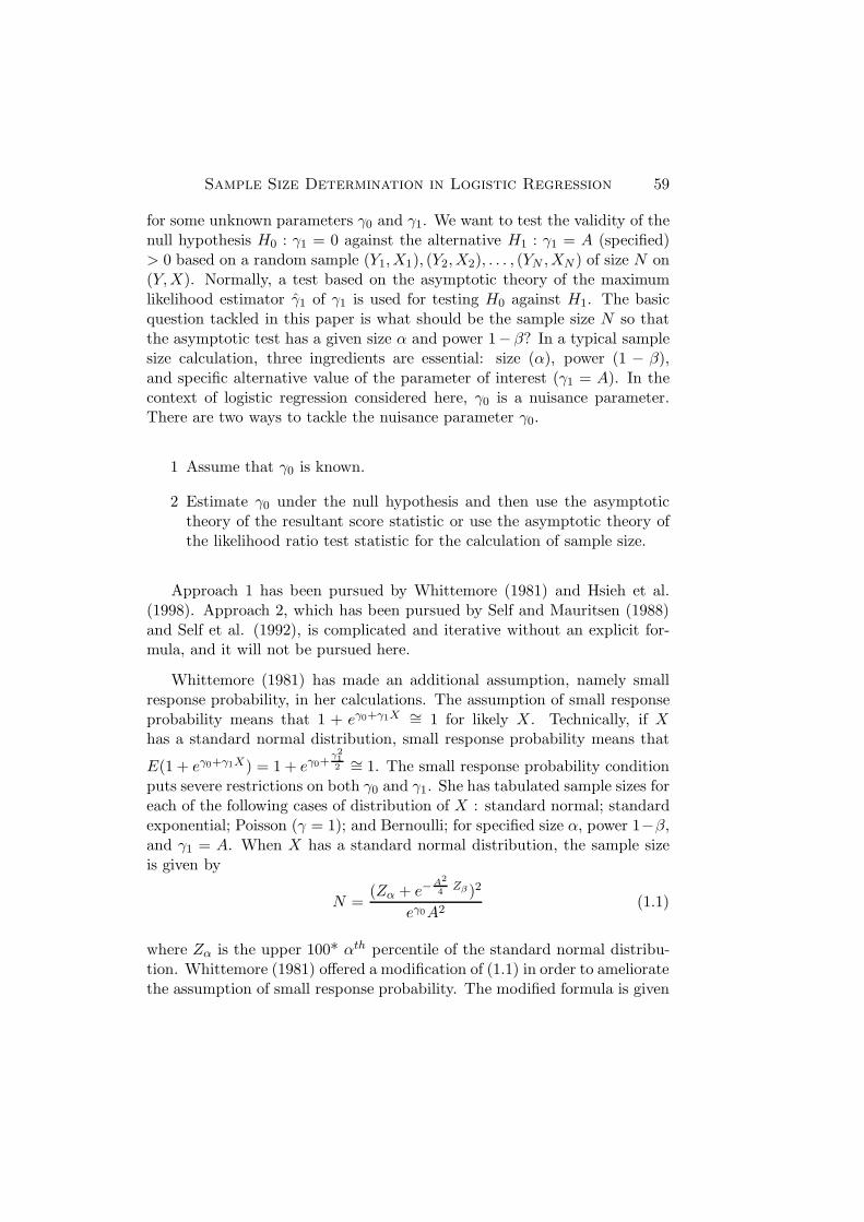
for some unknown parameters γ0 and γ1. We want to test the validity of thenull hypothesis H0 : γ1 = 0 against the alternative H1 : γ1 = A (specified)> 0 based on a random sample (Y1,X1), (Y2,X2), . . . , (YN ,XN ) of size N on(Y,X). Normally, a test based on the asymptotic theory of the maximumlikelihood estimator γ1 of γ1 is used for testing H0 against H1. The basicquestion tackled in this paper is what should be the sample size N so thatthe asymptotic test has a given size α and power 1− β? In a typical samplesize calculation, three ingredients are essential: size (α), power (1 − β),and specific alternative value of the parameter of interest (γ1 = A). In thecontext of logistic regression considered here, γ0 is a nuisance parameter.There are two ways to tackle the nuisance parameter γ0.

1 Assume that γ0 is known.

2 Estimate γ0 under the null hypothesis and then use the asymptotictheory of the resultant score statistic or use the asymptotic theory ofthe likelihood ratio test statistic for the calculation of sample size.

Approach 1 has been pursued by Whittemore (1981) and Hsieh et al.(1998). Approach 2, which has been pursued by Self and Mauritsen (1988)and Self et al. (1992), is complicated and iterative without an explicit for-mula, and it will not be pursued here.

Whittemore (1981) has made an additional assumption, namely smallresponse probability, in her calculations. The assumption of small responseprobability means that 1 + eγ0+γ1X ∼= 1 for likely X. Technically, if X

has a standard normal distribution, small response probability means that

E(1 + eγ0+γ1X) = 1 + eγ0+γ212 ∼= 1. The small response probability condition

puts severe restrictions on both γ0 and γ1. She has tabulated sample sizes foreach of the following cases of distribution of X : standard normal; standardexponential; Poisson (γ = 1); and Bernoulli; for specified size α, power 1−β,and γ1 = A. When X has a standard normal distribution, the sample sizeis given by

N =(Zα + e−

A2

4Zβ )2

eγ0A2(1.1)

where Zα is the upper 100* αth percentile of the standard normal distribu-tion. Whittemore (1981) offered a modification of (1.1) in order to amelioratethe assumption of small response probability. The modified formula is given

60 M. Khorshed Alam, M. Bhaskara Rao and Fu-Chih Cheng

by

N =

(

Zα + e−A2

4 Zβ

)2

eγ0A2∗

1 + 2eγ0 ∗ [1 + (1 + A2) e5A2

4 ]

(1 + 2 eγ0

(1.2)

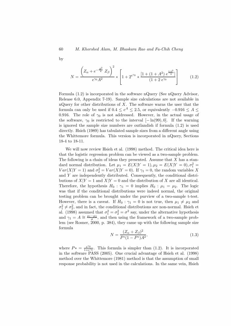
Formula (1.2) is incorporated in the software nQuery (See nQuery Advisor,Release 6.0, Appendix 7-19). Sample size calculations are not available innQuery for other distributions of X. The software warns the user that theformula can only be used if 0.4 ≤ eA ≤ 2.5, or equivalently −0.916 ≤ A ≤0.916. The role of γ0 is not addressed. However, in the actual usage ofthe software, γ0 is restricted to the interval [− ln(99), 0]. If the warningis ignored the sample size numbers are outlandish if formula (1.2) is useddirectly. Hsieh (1989) has tabulated sample sizes from a different angle usingthe Whittemore formula. This version is incorporated in nQuery, Sections18-4 to 18-11.

We will now review Hsieh et al. (1998) method. The critical idea here isthat the logistic regression problem can be viewed as a two-sample problem.The following is a chain of ideas they presented. Assume that X has a stan-dard normal distribution. Let µ1 = E(X|Y = 1), µ2 = E(X|Y = 0), σ2

1 =V ar(X|Y = 1) and σ2

2 = V ar(X|Y = 0). If γ1 = 0, the random variables X

and Y are independently distributed. Consequently, the conditional distri-butions of X|Y = 1 and X|Y = 0 and the distribution of X are all identical.Therefore, the hypothesis H0 : γ1 = 0 implies H0 : µ1 = µ2. The logicwas that if the conditional distributions were indeed normal, the originaltesting problem can be brought under the purview of a two-sample t-test.However, there is a caveat. If H0 : γ1 = 0 is not true, then µ1 6= µ2 andσ2

1 6= σ22 , and in fact, the conditional distributions are non-normal. Hsieh et

al. (1998) assumed that σ21 = σ2

2 = σ2 say, under the alternative hypothesisand γ1 = A ∼= µ1−µ2

σ, and then using the framework of a two-sample prob-

lem (see Rosner, 2000, p. 384), they came up with the following sample sizeformula

N =(Zα + Zβ)2

P ∗(1 − P ∗)A2, (1.3)

where P∗ = eγ0

1+eγ0. This formula is simpler than (1.2). It is incorporated

in the software PASS (2005). One crucial advantage of Hsieh et al. (1998)method over the Whittemore (1981) method is that the assumption of smallresponse probability is not used in the calculations. In the same vein, Hsieh


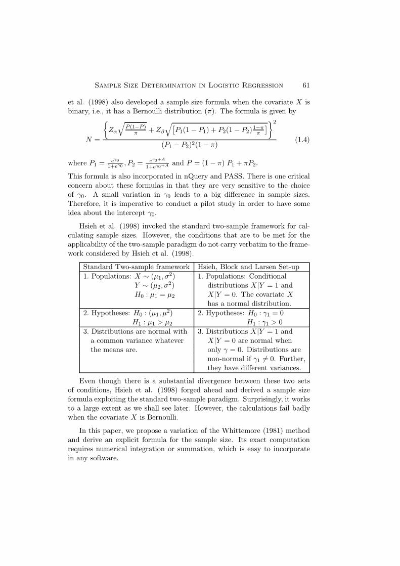
et al. (1998) also developed a sample size formula when the covariate X isbinary, i.e., it has a Bernoulli distribution (π). The formula is given by

N =

{

Zα

√

P (1−P )π

+ Zβ

√

[

P1(1 − P1) + P2(1 − P2)1−π

π

]

}2

(P1 − P2)2(1 − π)(1.4)

where P1 = eγ0

1+eγ0 , P2 = eγ0+A

1+eγ0+A and P = (1 − π) P1 + πP2.

This formula is also incorporated in nQuery and PASS. There is one criticalconcern about these formulas in that they are very sensitive to the choiceof γ0. A small variation in γ0 leads to a big difference in sample sizes.Therefore, it is imperative to conduct a pilot study in order to have someidea about the intercept γ0.

Hsieh et al. (1998) invoked the standard two-sample framework for cal-culating sample sizes. However, the conditions that are to be met for theapplicability of the two-sample paradigm do not carry verbatim to the frame-work considered by Hsieh et al. (1998).

Standard Two-sample framework Hsieh, Block and Larsen Set-up

1. Populations: X ∼ (µ1, σ2) 1. Populations: Conditional

Y ∼ (µ2, σ2) distributions X|Y = 1 and

H0 : µ1 = µ2 X|Y = 0. The covariate X

has a normal distribution.

2. Hypotheses: H0 : (µ1, µ2) 2. Hypotheses: H0 : γ1 = 0

H1 : µ1 > µ2 H1 : γ1 > 0

3. Distributions are normal with 3. Distributions X|Y = 1 anda common variance whatever X|Y = 0 are normal whenthe means are. only γ = 0. Distributions are

non-normal if γ1 6= 0. Further,they have different variances.

Even though there is a substantial divergence between these two setsof conditions, Hsieh et al. (1998) forged ahead and derived a sample sizeformula exploiting the standard two-sample paradigm. Surprisingly, it worksto a large extent as we shall see later. However, the calculations fail badlywhen the covariate X is Bernoulli.

In this paper, we propose a variation of the Whittemore (1981) methodand derive an explicit formula for the sample size. Its exact computationrequires numerical integration or summation, which is easy to incorporatein any software.


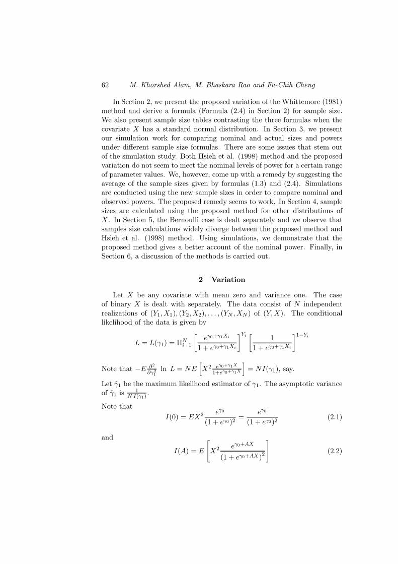
In Section 2, we present the proposed variation of the Whittemore (1981)method and derive a formula (Formula (2.4) in Section 2) for sample size.We also present sample size tables contrasting the three formulas when thecovariate X has a standard normal distribution. In Section 3, we presentour simulation work for comparing nominal and actual sizes and powersunder different sample size formulas. There are some issues that stem outof the simulation study. Both Hsieh et al. (1998) method and the proposedvariation do not seem to meet the nominal levels of power for a certain rangeof parameter values. We, however, come up with a remedy by suggesting theaverage of the sample sizes given by formulas (1.3) and (2.4). Simulationsare conducted using the new sample sizes in order to compare nominal andobserved powers. The proposed remedy seems to work. In Section 4, samplesizes are calculated using the proposed method for other distributions ofX. In Section 5, the Bernoulli case is dealt separately and we observe thatsamples size calculations widely diverge between the proposed method andHsieh et al. (1998) method. Using simulations, we demonstrate that theproposed method gives a better account of the nominal power. Finally, inSection 6, a discussion of the methods is carried out.

2 Variation

Let X be any covariate with mean zero and variance one. The caseof binary X is dealt with separately. The data consist of N independentrealizations of (Y1,X1), (Y2,X2), . . . , (YN ,XN ) of (Y,X). The conditionallikelihood of the data is given by

L = L(γ1) = ΠNi=1

[

eγ0+γ1Xi

1 + eγ0+γ1Xi

]Yi[

1

1 + eγ0+γ1Xi

]1−Yi

Note that −E ∂2

∂γ21

ln L = NE[

X2 eγ0+γ1X

1+eγ0+γ1X

]

= NI(γ1), say.

Let γ1 be the maximum likelihood estimator of γ1. The asymptotic varianceof γ1 is 1

N I(γ1) .

Note that

I(0) = EX2 eγ0

(1 + eγ0)2=

eγ0

(1 + eγ0)2(2.1)

and

I(A) = E

[

X2 eγ0+AX

(1 + eγ0+AX)2

]

(2.2)


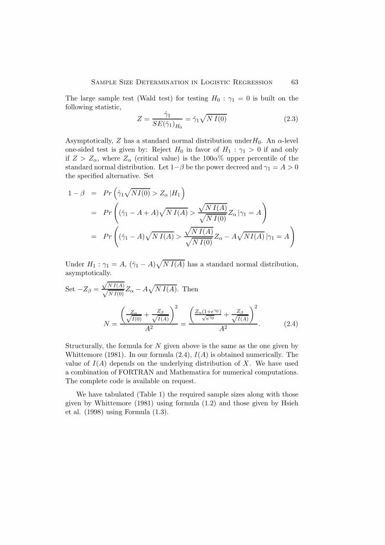
The large sample test (Wald test) for testing H0 : γ1 = 0 is built on thefollowing statistic,

Z =γ1

SE(γ1)H0

= γ1

√

N I(0) (2.3)

Asymptotically, Z has a standard normal distribution underH0. An α-levelone-sided test is given by: Reject H0 in favor of H1 : γ1 > 0 if and onlyif Z > Zα, where Zα (critical value) is the 100α% upper percentile of thestandard normal distribution. Let 1−β be the power decreed and γ1 = A > 0the specified alternative. Set

1 − β = Pr(

γ1

√

NI(0) > Zα |H1

)

= Pr

(

(γ1 − A + A)√

N I(A) >

√

N I(A)√

N I(0)Zα |γ1 = A

)

= Pr

(

(γ1 − A)√

N I(A) >

√

N I(A)√

N I(0)Zα − A

√

NI(A) |γ1 = A

)

Under H1 : γ1 = A, (γ1 − A)√

N I(A) has a standard normal distribution,asymptotically.

Set −Zβ =

√N I(A)√N I(0)

Zα − A√

N I(A). Then

N =

(

Zα√I(0)

+Zβ√I(A)

)2

A2=

(

Zα(1+eγ0 )√

eγ0+

Zβ√I(A)

)2

A2. (2.4)

Structurally, the formula for N given above is the same as the one given byWhittemore (1981). In our formula (2.4), I(A) is obtained numerically. Thevalue of I(A) depends on the underlying distribution of X. We have useda combination of FORTRAN and Mathematica for numerical computations.The complete code is available on request.

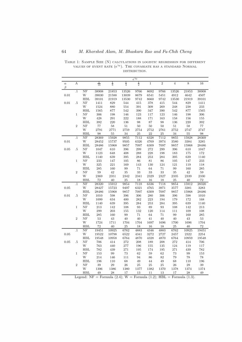
We have tabulated (Table 1) the required sample sizes along with thosegiven by Whittemore (1981) using formula (1.2) and those given by Hsiehet al. (1998) using Formula (1.3).


Table 1: Sample Size (N) calculations in logistic regression for differentvalues of event rate (eγ0). The covariate has a standard Normal

distribution.

eγ0

α A 116

18

14

12

1 2 4 8 16β

.1 NF 38908 21853 13526 9766 8692 9766 13526 21853 389080.01 W 39030 21588 13039 8679 6541 5451 4912 4642 4507

HBL 39101 21919 13530 9742 8660 9742 13530 21919 391010.01 .5 NF 1411 829 544 415 378 415 544 829 1411

W 1524 880 554 391 309 269 248 238 233HBL 1565 877 542 390 347 390 542 877 1565

1 NF 306 198 146 123 117 123 146 198 306W 428 291 222 188 171 163 158 156 155HBL 392 220 136 98 87 98 136 220 392

2 NF 77 58 51 50 50 50 51 58 77W 2791 2771 2759 2754 2752 2761 2752 2747 2747HBL 98 55 34 25 22 25 34 55 98

.1 NF 28369 15928 9855 7112 6328 7112 9855 15928 283690.01 W 28452 15737 9505 6326 4769 3974 3580 3384 3285

HBL 28486 15968 9857 7097 6309 7097 9857 15968 284860.05 .5 NF 1047 610 396 299 272 299 396 610 1047

W 1123 648 408 288 228 198 183 175 172HBL 1140 639 395 284 253 284 395 639 1140

1 NF 233 147 105 86 81 86 105 147 233W 325 221 169 143 130 124 121 119 118HBL 285 160 99 71 64 71 99 160 285

2 NF 59 42 35 33 33 33 35 42 59W 2369 2351 2342 2341 2329 2327 2335 2339 2330HBL 72 40 25 18 16 18 25 40 72

.1 NF 28320 15912 9854 7118 6336 7118 9854 15912 283200.05 W 28427 15723 9497 6321 4765 3971 3577 3381 3283

HBL 28486 15968 9857 7097 6309 7097 9857 15968 284860.01 .5 NF 1010 598 396 306 280 306 396 598 1010

W 1099 634 400 282 223 194 179 172 168HBL 1140 639 395 284 253 284 395 639 1140

1 NF 213 142 108 93 89 93 108 142 213W 299 203 155 132 120 114 111 109 108HBL 285 160 99 71 64 71 99 160 285

2 NF 53 43 40 40 41 40 40 43 53W 1724 1711 1704 1704 1697 1696 1700 1696 1704HBL 72 40 25 18 16 18 25 40 72

.1 NF 19451 10925 6762 4883 4346 4883 6762 10925 194510.05 W 19522 10798 6522 4341 3272 2727 2457 2322 2254

HBL 19548 10958 6764 4870 4328 4870 6764 10959 195480.05 .5 NF 706 414 272 208 189 208 272 414 706

W 763 440 277 196 155 135 124 119 117HBL 782 439 271 195 174 195 271 439 782

1 NF 153 99 73 62 59 62 73 99 153W 214 146 111 94 86 82 79 78 78HBL 196 110 68 49 44 49 68 110 196

2 NF 39 29 26 25 25 25 26 29 39W 1396 1386 1380 1377 1382 1370 1378 1374 1374HBL 49 28 17 13 11 13 17 28 49

Legend: NF = Formula (2.4); W = Formula (1.2); HBL = Formula (1.3).


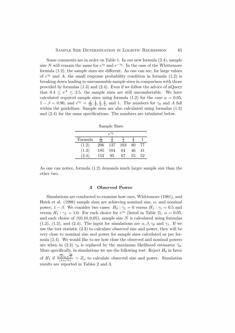
Some comments are in order on Table 1. In our new formula (2.4), samplesize N will remain the same for eγ0 and e−γ0 . In the case of the Whittemoreformula (1.2), the sample sizes are different. As one can see, for large valuesof eγ0 and A, the small response probability condition in formula (1.2) isbreaking down leading to unreasonable sample sizes in comparison with thoseprovided by formulas (1.3) and (2.4). Even if we follow the advice of nQuerythat 0.4 ≤ eA ≤ 2.5, the sample sizes are still uncomfortable. We havecalculated required sample sizes using formula (1.2) for the case α = 0.05,1 − β = 0.90, and eγ0 = 1

16 , 18 , 1

4 , 12 , and 1. The numbers for γ0 and A fall

within the guidelines. Sample sizes are also calculated using formulas (1.3)and (2.4) for the same specifications. The numbers are tabulated below.

Sample Sizes

eγ0

Formula 116

18

14

12 1

(1.2) 206 137 103 80 77(1.3) 185 104 64 46 41(2.4) 152 95 67 55 52

As one can notice, formula (1.2) demands much larger sample size than theother two.

3 Observed Power

Simulations are conducted to examine how ours, Whittemore (1981), andHsieh et al. (1998) sample sizes are achieving nominal size, α, and nominalpower, 1 − β. We consider two cases: H0 : γ1 = 0 versus H1 : γ1 = 0.5 andversus H1 : γ1 = 1.0. For each choice for eγ0 (listed in Table 2), α = 0.05,and each choice of β(0.10, 0.05), sample size N is calculated using formulas(1.2), (1.3), and (2.4). The input for simulations are α, β, γ0 and γ1. If weuse the test statistic (2.3) to calculate observed size and power, they will bevery close to nominal size and power for sample sizes calculated as per for-mula (2.4). We would like to see how close the observed and nominal powersare when in (2.3) γ0 is replaced by the maximum likelihood estimator γ0.More specifically, in simulations we use the following test: Reject H0 in favor

of H1 if√

Nγ1 eγ02

(1+eγ0 )> Zα to calculate observed size and power. Simulation

results are reported in Tables 2 and 3.

66M

.K

horsh

edA

lam

,M

.Bhask

ara

Rao

and

Fu-C

hih

Cheng

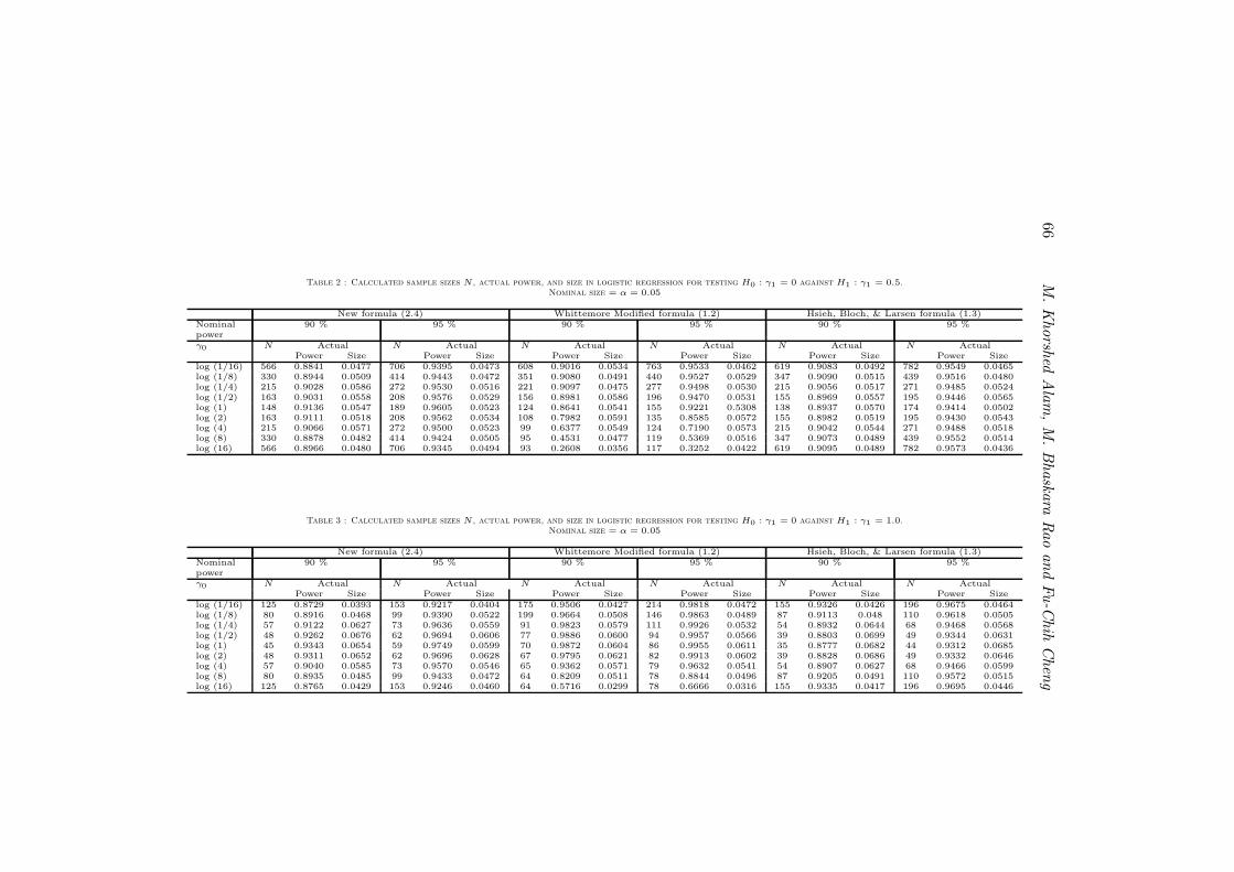
Table 2 : Calculated sample sizes N , actual power, and size in logistic regression for testing H0 : γ1 = 0 against H1 : γ1 = 0.5.Nominal size = α = 0.05

New formula (2.4) Whittemore Modified formula (1.2) Hsieh, Bloch, & Larsen formula (1.3)Nominal 90 % 95 % 90 % 95 % 90 % 95 %powerγ0 N Actual N Actual N Actual N Actual N Actual N Actual

Power Size Power Size Power Size Power Size Power Size Power Sizelog (1/16) 566 0.8841 0.0477 706 0.9395 0.0473 608 0.9016 0.0534 763 0.9533 0.0462 619 0.9083 0.0492 782 0.9549 0.0465log (1/8) 330 0.8944 0.0509 414 0.9443 0.0472 351 0.9080 0.0491 440 0.9527 0.0529 347 0.9090 0.0515 439 0.9516 0.0480log (1/4) 215 0.9028 0.0586 272 0.9530 0.0516 221 0.9097 0.0475 277 0.9498 0.0530 215 0.9056 0.0517 271 0.9485 0.0524log (1/2) 163 0.9031 0.0558 208 0.9576 0.0529 156 0.8981 0.0586 196 0.9470 0.0531 155 0.8969 0.0557 195 0.9446 0.0565log (1) 148 0.9136 0.0547 189 0.9605 0.0523 124 0.8641 0.0541 155 0.9221 0.5308 138 0.8937 0.0570 174 0.9414 0.0502log (2) 163 0.9111 0.0518 208 0.9562 0.0534 108 0.7982 0.0591 135 0.8585 0.0572 155 0.8982 0.0519 195 0.9430 0.0543log (4) 215 0.9066 0.0571 272 0.9500 0.0523 99 0.6377 0.0549 124 0.7190 0.0573 215 0.9042 0.0544 271 0.9488 0.0518log (8) 330 0.8878 0.0482 414 0.9424 0.0505 95 0.4531 0.0477 119 0.5369 0.0516 347 0.9073 0.0489 439 0.9552 0.0514log (16) 566 0.8966 0.0480 706 0.9345 0.0494 93 0.2608 0.0356 117 0.3252 0.0422 619 0.9095 0.0489 782 0.9573 0.0436

Table 3 : Calculated sample sizes N , actual power, and size in logistic regression for testing H0 : γ1 = 0 against H1 : γ1 = 1.0.Nominal size = α = 0.05

New formula (2.4) Whittemore Modified formula (1.2) Hsieh, Bloch, & Larsen formula (1.3)Nominal 90 % 95 % 90 % 95 % 90 % 95 %powerγ0 N Actual N Actual N Actual N Actual N Actual N Actual

Power Size Power Size Power Size Power Size Power Size Power Sizelog (1/16) 125 0.8729 0.0393 153 0.9217 0.0404 175 0.9506 0.0427 214 0.9818 0.0472 155 0.9326 0.0426 196 0.9675 0.0464log (1/8) 80 0.8916 0.0468 99 0.9390 0.0522 199 0.9664 0.0508 146 0.9863 0.0489 87 0.9113 0.048 110 0.9618 0.0505log (1/4) 57 0.9122 0.0627 73 0.9636 0.0559 91 0.9823 0.0579 111 0.9926 0.0532 54 0.8932 0.0644 68 0.9468 0.0568log (1/2) 48 0.9262 0.0676 62 0.9694 0.0606 77 0.9886 0.0600 94 0.9957 0.0566 39 0.8803 0.0699 49 0.9344 0.0631log (1) 45 0.9343 0.0654 59 0.9749 0.0599 70 0.9872 0.0604 86 0.9955 0.0611 35 0.8777 0.0682 44 0.9312 0.0685log (2) 48 0.9311 0.0652 62 0.9696 0.0628 67 0.9795 0.0621 82 0.9913 0.0602 39 0.8828 0.0686 49 0.9332 0.0646log (4) 57 0.9040 0.0585 73 0.9570 0.0546 65 0.9362 0.0571 79 0.9632 0.0541 54 0.8907 0.0627 68 0.9466 0.0599log (8) 80 0.8935 0.0485 99 0.9433 0.0472 64 0.8209 0.0511 78 0.8844 0.0496 87 0.9205 0.0491 110 0.9572 0.0515log (16) 125 0.8765 0.0429 153 0.9246 0.0460 64 0.5716 0.0299 78 0.6666 0.0316 155 0.9335 0.0417 196 0.9695 0.0446


From Tables 2 and 3, it is clear that the Whittemore formula (1.2) is notgiving actual powers close to the nominal one as we move away from smallγ0 to large γ0. This study provides a clear warning to what happens if weignore the small response probability condition.

New formula (2.4) and formula (1.3) are also not up to the mark. Forsmall and large values of γ0, New formula (2.4) is giving significantly lowerpowers than the nominal ones. For middle values of γ0 formula (1.3) isgiving significantly lower powers than the nominal ones. This is becausethe formulas are derived by assuming γ0 is known, whereas in simulationsestimated γ0 is used. In the case of formula (1.3), the assumption thatσ2

1 = σ22 = σ2 and A ∼= µ1−µ2

σ, which are not valid, might be playing a role

in lower observed powers. For example, when γ0 = 3, γ1 = A = 1, µ1 =0.05621, µ2 = 0.75642, σ2

1 = 0.95000, and σ22 = 1.05810. If we take σ2 to be

the average of σ21 and σ2

2, we have A ∼= µ1−µ2

σ= 0.80609 but A = 1.

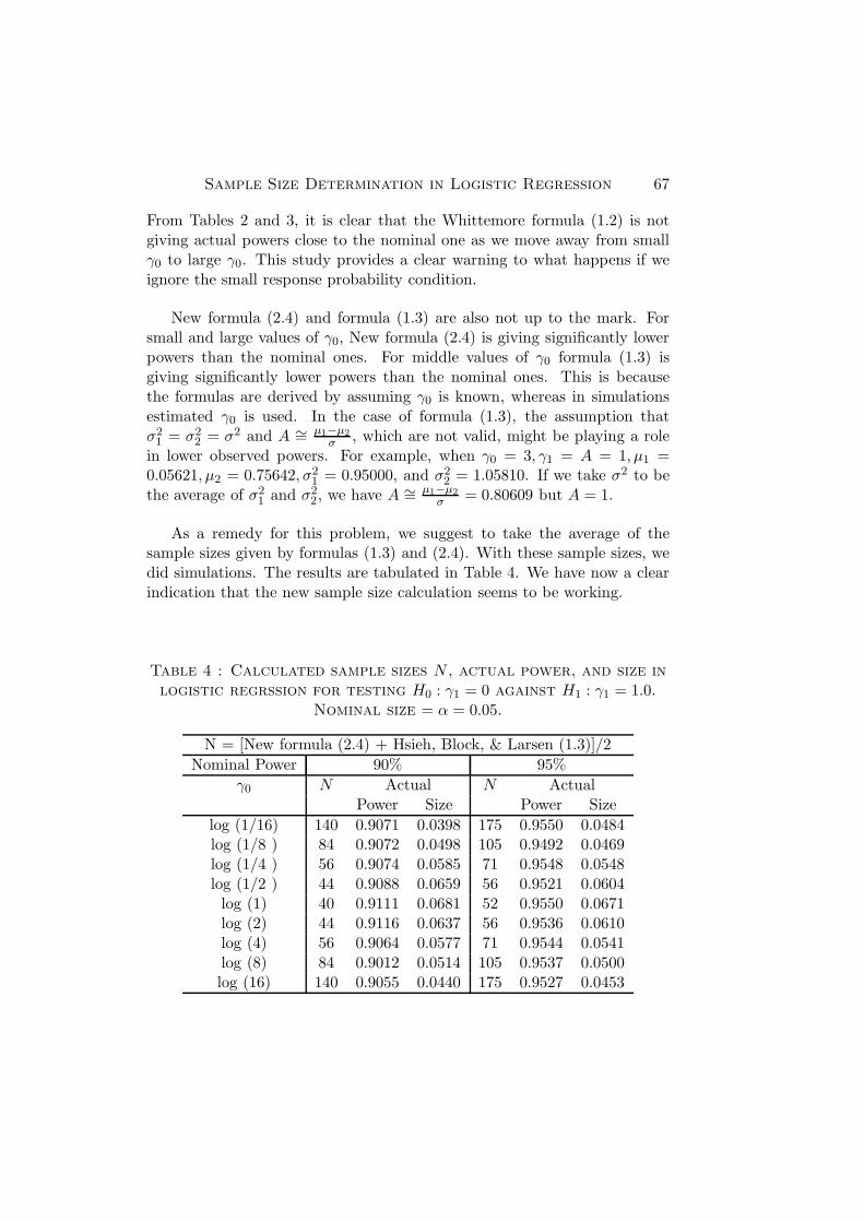
As a remedy for this problem, we suggest to take the average of thesample sizes given by formulas (1.3) and (2.4). With these sample sizes, wedid simulations. The results are tabulated in Table 4. We have now a clearindication that the new sample size calculation seems to be working.

Table 4 : Calculated sample sizes N , actual power, and size inlogistic regrssion for testing H0 : γ1 = 0 against H1 : γ1 = 1.0.

Nominal size = α = 0.05.

N = [New formula (2.4) + Hsieh, Block, & Larsen (1.3)]/2

Nominal Power 90% 95%

γ0 N Actual N ActualPower Size Power Size

log (1/16) 140 0.9071 0.0398 175 0.9550 0.0484log (1/8 ) 84 0.9072 0.0498 105 0.9492 0.0469log (1/4 ) 56 0.9074 0.0585 71 0.9548 0.0548log (1/2 ) 44 0.9088 0.0659 56 0.9521 0.0604log (1) 40 0.9111 0.0681 52 0.9550 0.0671log (2) 44 0.9116 0.0637 56 0.9536 0.0610log (4) 56 0.9064 0.0577 71 0.9544 0.0541log (8) 84 0.9012 0.0514 105 0.9537 0.0500log (16) 140 0.9055 0.0440 175 0.9527 0.0453


4 Other Distributions

We look at three other cases for the distribution of the covariate X.

1. X has a standardized exponential distribution, i.e.,X = U − 1, whereU has a standard exponential distribution (Exp(λ) ( with λ = 1).

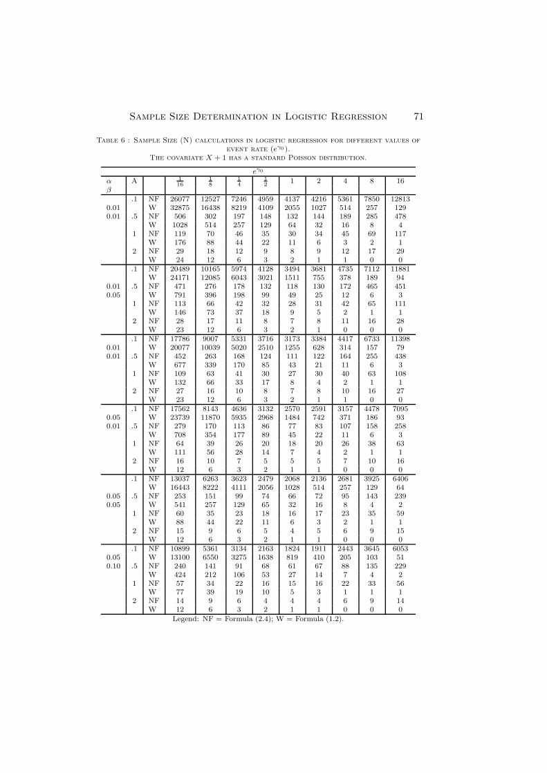
2. X has a standardized Poisson distribution, i.e.,X = U − 1, where U

has a Poisson distribution with mean unity.

3. X has a Bernoulli distribution (π).

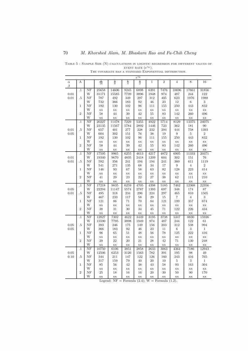
In Cases 1 and 2, the entity I(0), under H0 : γ1 = 0 remains the same asin (2.1), and the test statistic also remains the same as in (2.3). The formulafor N structurally also remains the same as in (2.4). The only difference liesin the computation of I(A), which is extracted numerically from (2.2) usingthe assumed distribution of X. The sample sizes as per formula (2.4) aregiven in Tables 5, 6, and 7 along side the Whittemore(1981) numbers. Inthe case of Bernoulli distribution, we have an explicit formula for I(A) givenby,

I(A) = π

[

eγ0+A

(1 + eγ0+A)2

]

. (4.1)

The Whittemore (1981) formula (1.2) can not be used for certain values ofA in the exponential case as the integral involved in the formula does notexist. The symbol (xx) in Table 5 indicates such a contingency. Hsieh et al.(1998) have not considered these distributions.

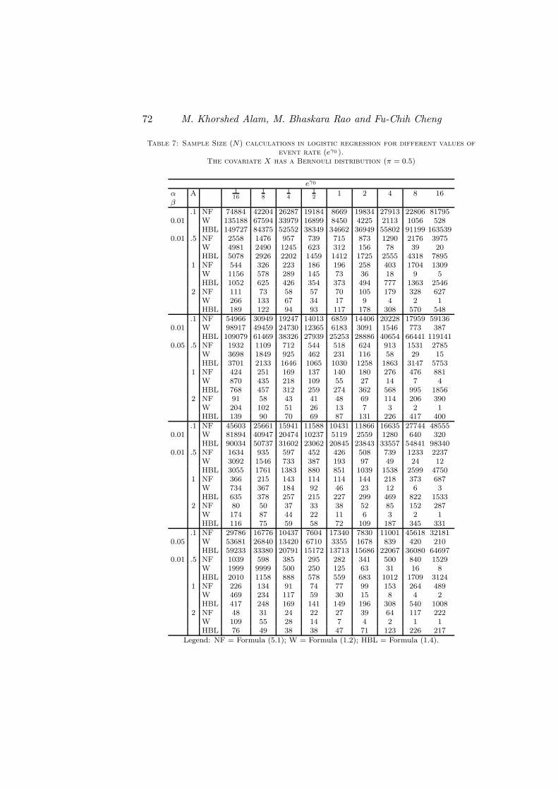
5 The Bernoulli Case

In the case of Bernoulli X with success probability π, we have calculatedrequired sample sizes using formula (1.4) of Hsieh et al. (1998) and thefollowing formula stemming from our proposed method:

N =

(

Zα√I(0)

+Zβ√I(A)

)2

A2=

(

Zα(1+eγ0 )√

π∗eγ0+

Zβ√I(A)

)2

A2, (5.1)

where I(A) is given by (2.2).


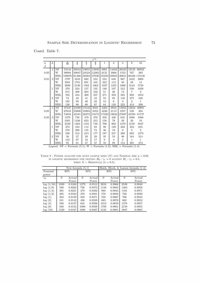
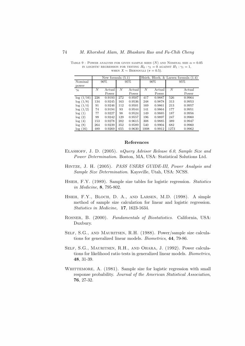
The sample sizes differ considerably with formula (1.4) giving higher num-bers. We conducted simulations (10,000 times) to check which sample sizeprovides a good account of the nominal power. We have tabulated the sam-ple sizes in Table 7 and simulation work in Tables 8 and 9. From Tables 8and 9, it is clear that formula (1.4) gives more power than what we havesought with larger sample size it provides.

6 Discussion

Sample size formulas are available in the literature in the context oflogistic regression with a single covariate. Formula (1.2) has been derivedby Whittemore (1981) under the assumption of small response probability.Formula (1.3) has been derived by Hsieh et al. (1998) by formulating thehypothesis testing problem as a two-sample problem. In this paper, wepropose a new way for calculating sample size given by formula (2.4). Wetabulate below the approaches pursued by the three contributors in thiscontext.

Whittemore (1981) Hsieh, Block and Larsen New Approach(1998)Method

Maximum Likelihood Two-sample problem Maximum LikelihoodAssumption

Small response The conditional distributions Noneprobability of X |Y = 1 and X |Y = 0

have normal distributionswith equal variance underH1 (Not true)

We compare all three formulas via simulations to see how close the ob-served and nominal powers are. When the covariate is Bernoulli, the newmethod provides a better account of nominal power than the method pro-posed by Hsieh et al. (1998). Unlike Hsieh et al. (1988) method, which haslimitations on X, our method is applicable whatever may be the distributionof the covariate X.


Table 5 : Sample Size (N) calculations in logistic regression for different values ofevent rate (eγ0 ).

The covariate has a standard Exponential distribution.

eγ0

α A 116

18

14

12

1 2 4 8 16β

.1 NF 25658 14606 9245 6898 6391 7476 10696 17661 318560.01 W 31171 15585 7739 3896 1948 974 487 244 1220.01 .5 NF 787 492 349 297 312 405 623 1976 1988

W 732 366 183 92 46 23 12 6 31 NF 192 130 102 96 111 155 250 443 832

W xx xx xx xx xx xx xx xx xx2 NF 58 44 39 42 55 83 142 260 496

W xx xx xx xx xx xx xx xx xx.1 NF 20227 11478 7229 5355 4922 5714 8129 13375 24075

W 23135 11567 5784 2892 1446 723 362 181 900.01 .5 NF 657 401 277 228 232 294 444 758 13930.05 W 604 302 151 76 38 19 9 5 2

1 NF 192 130 102 96 111 155 250 443 832W xx xx xx xx xx xx xx xx xx


.1 NF 17595 9965 6255 4613 4217 4872 6905 11333 203710.01 W 19340 9670 4835 2418 1209 604 302 151 760.01 .5 NF 592 356 241 194 194 241 360 611 1119

W 541 271 135 68 34 17 9 4 21 NF 146 93 67 58 63 82 128 223 414



0.05 W 22294 11147 5574 2787 1393 697 348 174 870.01 .5 NF 495 318 234 296 224 297 465 810 1505

W 467 233 117 58 29 15 7 4 31 NF 121 86 71 70 84 121 199 357 674



W 15590 7795 3898 1949 974 487 244 122 610.05 .5 NF 393 246 175 149 156 203 312 538 9940.05 W 366 183 92 46 23 11 6 3 1



.1 NF 10750 6106 3851 2858 2633 3063 4364 7186 129430.05 W 12506 6253 3126 1563 782 391 195 98 490.10 .5 NF 344 211 147 122 126 160 243 416 765

W 317 159 79 40 20 10 5 3 11 NF 85 56 42 38 43 58 93 163 304


W xx xx xx xx xx xx xx xx xx

Legend: NF = Formula (2.4); W = Formula (1.2).


Table 6 : Sample Size (N) calculations in logistic regression for different values ofevent rate (eγ0 ).

The covariate X + 1 has a standard Poisson distribution.

eγ0

α A 116

18

14

12

1 2 4 8 16β

.1 NF 26077 12527 7246 4959 4137 4216 5361 7850 128130.01 W 32875 16438 8219 4109 2055 1027 514 257 1290.01 .5 NF 506 302 197 148 132 144 189 285 478

W 1028 514 257 129 64 32 16 8 41 NF 119 70 46 35 30 34 45 69 117

W 176 88 44 22 11 6 3 2 12 NF 29 18 12 9 8 9 12 17 29

W 24 12 6 3 2 1 1 0 0.1 NF 20489 10165 5974 4128 3494 3681 4735 7112 11881

W 24171 12085 6043 3021 1511 755 378 189 940.01 .5 NF 471 276 178 132 118 130 172 465 4510.05 W 791 396 198 99 49 25 12 6 3

1 NF 113 66 42 32 28 31 42 65 111W 146 73 37 18 9 5 2 1 1

2 NF 28 17 11 8 7 8 11 16 28W 23 12 6 3 2 1 0 0 0

.1 NF 17786 9007 5331 3716 3173 3384 4417 6733 113980.01 W 20077 10039 5020 2510 1255 628 314 157 790.01 .5 NF 452 263 168 124 111 122 164 255 438

W 677 339 170 85 43 21 11 6 31 NF 109 63 41 30 27 30 40 63 108

W 132 66 33 17 8 4 2 1 12 NF 27 16 10 8 7 8 10 16 27

W 23 12 6 3 2 1 1 0 0.1 NF 17562 8143 4636 3132 2570 2591 3157 4478 7095

0.05 W 23739 11870 5935 2968 1484 742 371 186 930.01 .5 NF 279 170 113 86 77 83 107 158 258

W 708 354 177 89 45 22 11 6 31 NF 64 39 26 20 18 20 26 38 63

W 111 56 28 14 7 4 2 1 12 NF 16 10 7 5 5 5 7 10 16

W 12 6 3 2 1 1 0 0 0.1 NF 13037 6263 3623 2479 2068 2136 2681 3925 6406

W 16443 8222 4111 2056 1028 514 257 129 640.05 .5 NF 253 151 99 74 66 72 95 143 2390.05 W 541 257 129 65 32 16 8 4 2

1 NF 60 35 23 18 16 17 23 35 59W 88 44 22 11 6 3 2 1 1

2 NF 15 9 6 5 4 5 6 9 15W 12 6 3 2 1 1 0 0 0

.1 NF 10899 5361 3134 2163 1824 1911 2443 3645 60530.05 W 13100 6550 3275 1638 819 410 205 103 510.10 .5 NF 240 141 91 68 61 67 88 135 229

W 424 212 106 53 27 14 7 4 21 NF 57 34 22 16 15 16 22 33 56

W 77 39 19 10 5 3 1 1 12 NF 14 9 6 4 4 4 6 9 14

W 12 6 3 2 1 1 0 0 0

Legend: NF = Formula (2.4); W = Formula (1.2).


Table 7: Sample Size (N) calculations in logistic regression for different values ofevent rate (eγ0 ).

The covariate X has a Bernouli distribution (π = 0.5)

eγ0

α A 116

18

14

12

1 2 4 8 16β

.1 NF 74884 42204 26287 19184 8669 19834 27913 22806 817950.01 W 135188 67594 33979 16899 8450 4225 2113 1056 528

HBL 149727 84375 52552 38349 34662 36949 55802 91199 1635390.01 .5 NF 2558 1476 957 739 715 873 1290 2176 3975

W 4981 2490 1245 623 312 156 78 39 20HBL 5078 2926 2202 1459 1412 1725 2555 4318 7895

1 NF 544 326 223 186 196 258 403 1704 1309W 1156 578 289 145 73 36 18 9 5HBL 1052 625 426 354 373 494 777 1363 2546

2 NF 111 73 58 57 70 105 179 328 627W 266 133 67 34 17 9 4 2 1HBL 189 122 94 93 117 178 308 570 548

.1 NF 54966 30949 19247 14013 6859 14406 20228 17959 591360.01 W 98917 49459 24730 12365 6183 3091 1546 773 387

HBL 109079 61469 38326 27939 25253 28886 40654 66441 1191410.05 .5 NF 1932 1109 712 544 518 624 913 1531 2785

W 3698 1849 925 462 231 116 58 29 15HBL 3701 2133 1646 1065 1030 1258 1863 3147 5753

1 NF 424 251 169 137 140 180 276 476 881W 870 435 218 109 55 27 14 7 4HBL 768 457 312 259 274 362 568 995 1856

2 NF 91 58 43 41 48 69 114 206 390W 204 102 51 26 13 7 3 2 1HBL 139 90 70 69 87 131 226 417 400

.1 NF 45603 25661 15941 11588 10431 11866 16635 27744 485550.01 W 81894 40947 20474 10237 5119 2559 1280 640 320

HBL 90034 50737 31602 23062 20845 23843 33557 54841 983400.01 .5 NF 1634 935 597 452 426 508 739 1233 2237

W 3092 1546 733 387 193 97 49 24 12HBL 3055 1761 1383 880 851 1039 1538 2599 4750

1 NF 366 215 143 114 114 144 218 373 687W 734 367 184 92 46 23 12 6 3HBL 635 378 257 215 227 299 469 822 1533

2 NF 80 50 37 33 38 52 85 152 287W 174 87 44 22 11 6 3 2 1HBL 116 75 59 58 72 109 187 345 331

.1 NF 29786 16776 10437 7604 17340 7830 11001 45618 321810.05 W 53681 26840 13420 6710 3355 1678 839 420 210

HBL 59233 33380 20791 15172 13713 15686 22067 36080 646970.01 .5 NF 1039 598 385 295 282 341 500 840 1529

W 1999 9999 500 250 125 63 31 16 8HBL 2010 1158 888 578 559 683 1012 1709 3124

1 NF 226 134 91 74 77 99 153 264 489W 469 234 117 59 30 15 8 4 2HBL 417 248 169 141 149 196 308 540 1008

2 NF 48 31 24 22 27 39 64 117 222W 109 55 28 14 7 4 2 1 1HBL 76 49 38 38 47 71 123 226 217



Contd. Table 7:

eγ0

α A 116

18

14

12

1 2 4 8 16β

.1 NF 54144 30544 19055 13939 6861 14494 20443 18135 600430.05 W 98094 49047 24524 12262 6131 3066 1553 767 383

HBL 109076 61466 38283 27936 25250 28883 40651 66438 1191380.01 .5 NF 1797 1043 682 534 524 648 967 1642 3009

W 3561 1781 891 445 223 112 56 28 14HBL 3698 2130 1563 1062 1027 1255 1860 3144 5750

1 NF 370 224 157 135 146 197 312 550 1029W 815 408 204 102 51 26 13 7 3HBL 765 454 309 257 271 359 565 992 1853

2 NF 72 49 41 43 55 85 148 275 528W 185 93 46 23 12 6 3 2 1HBL 136 88 68 67 84 129 223 414 399

.1 NF 37437 21099 13142 9591 5263 9916 13955 13844 408910.05 W 67616 33808 16904 8452 4226 2113 1057 529 264

HBL 74852 42181 26272 19172 17329 19822 27897 45593 817570.05 .5 NF 1279 738 479 370 358 436 645 1088 1988

W 2491 1246 623 312 156 78 39 20 10HBL 2539 1463 1101 730 706 862 1278 2159 3947

1 NF 272 163 112 93 98 129 202 352 655W 578 289 145 73 36 18 9 5 3HBL 526 313 213 177 187 247 389 682 1273

2 NF 56 37 29 29 35 53 90 164 314W 133 67 34 17 9 4 2 1 1HBL 95 61 47 47 59 89 154 285 274


Table 8 : Power analysis for given sample sizes (N) and Nominal size α = 0.05in logistic regression for testing H0 : γ1 = 0 against H1 : γ1 = 0.5,

when X ∼ Bernoulli (π = 0.5).

New formula (5.1) Hsieh, Bloch, & Larsen formula (1.4)Nominal 90% 95% 90% 95%powerγ0 N Actual N Actual N Actual N Actual

Power Power Power Powerlog (1/16) 1039 0.9160 1279 0.9512 2010 0.9868 2539 0.9949log (1/8) 598 0.9202 738 0.9472 1158 0.9884 1463 0.9958log (1/4) 385 0.9231 479 0.9492 888 0.9945 1101 0.9971log (1/2) 295 0.9163 370 0.9501 578 0.9893 730 0.9950log (1) 282 0.9129 358 0.9471 559 0.9867 706 0.9945log (2) 341 0.9142 436 0.9529 683 0.9976 862 0.9952log (4) 500 0.9137 645 0.9506 1012 0.9859 1278 0.9957log (8) 840 0.9152 1088 0.9508 1709 0.9861 2159 0.9955log (16) 1529 0.9197 1988 0.9497 3124 0.9881 3947 0.9965


Table 9 : Power analysis for given sample sizes (N) and Nominal size α = 0.05in logistic regression for testing H0 : γ1 = 0 against H1 : γ1 = 1,

when X ∼ Bernoulli (π = 0.5).

New formula (5.1) Hsieh, Bloch, & Larsen formula (1.4)Nominal 90% 95% 90% 95%powerγ0 N Actual N Actual N Actual N Actual

Power Power Power Powerlog (1/16) 226 0.9193 272 0.9507 417 0.9887 526 0.9964log (1/8) 134 0.9245 163 0.9536 248 0.9878 313 0.9953log (1/4) 91 0.9246 112 0.9501 169 0.9861 213 0.9957log (1/2) 74 0.9194 93 0.9544 141 0.9864 177 0.9951log (1) 77 0.9227 98 0.9524 149 0.9885 187 0.9956log (2) 99 0.9242 129 0.9557 196 0.9897 247 0.9960log (4) 153 0.9278 202 0.9615 308 0.9885 389 0.9947log (8) 264 0.9239 352 0.9589 540 0.9904 682 0.9960log (16) 489 0.9269 655 0.9630 1008 0.9912 1273 0.9962

References

Elashoff, J. D. (2005). nQuery Advisor Release 6.0, Sample Size and

Power Determination. Boston, MA, USA: Statistical Solutions Ltd.

Hintze, J. H. (2005). PASS USERS GUIDE-III, Power Analysis and

Sample Size Determination. Kaysville, Utah, USA: NCSS.

Hsieh, F.Y. (1989). Sample size tables for logistic regression. Statistics

in Medicine, 8, 795-802.

Hsieh, F.Y., Bloch, D. A., and Larsen, M.D. (1998). A simplemethod of sample size calculation for linear and logistic regression.Statistics in Medicine, 17, 1623-1634.

Rosner, B. (2000). Fundamentals of Biostatistics. California, USA:Duxbury.

Self, S.G., and Mauritsen, R.H. (1988). Power/sample size calcula-tions for generalized linear models. Biometrics, 44, 79-86.

Self, S.G., Mauritsen, R.H., and Ohara, J. (1992). Power calcula-tions for likelihood ratio tests in generalized linear models. Biometrics,48, 31-39.

Whittemore, A. (1981). Sample size for logistic regression with smallresponse probability. Journal of the American Statistical Association,76, 27-32.


M. Khorshed AlamCenter for Genome InformationDepartment of Environmental HealthUniversity of Cincinnati Medical CentreOH 45267U.S.A.E-mail: [email protected]

M. Bhaskara RaoCenter for Genome InformationDepartment of Environmental HealthUniversity of Cincinnati Medical CentreOH 45267U.S.A.E-mail: [email protected]

Fu-Chih ChengDepartment of StatisticsNorth Dakota State UniversityFargo, ND 58102U.S.A.E-mail: [email protected]

Paper received November 2007; revised November 2008.

Sample size determination in logistic · PDF fileSample Size Determination in Logistic...

Documents

Transcript of Sample size determination in logistic · PDF fileSample Size Determination in Logistic...