Efficient Logistic Regression with Stochastic Gradient Descent –

part 2

William Cohen

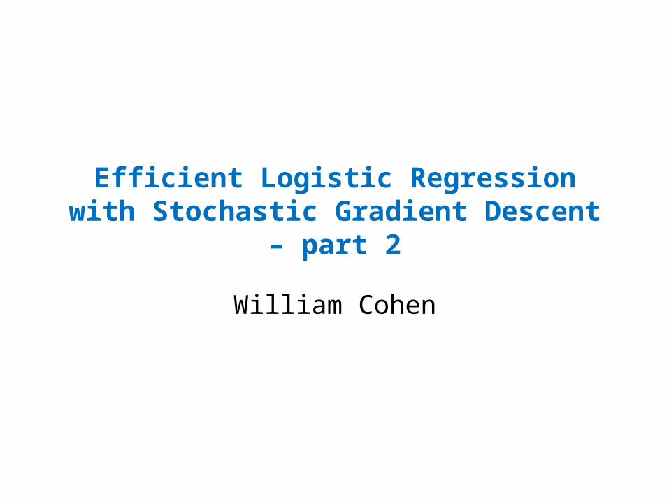
Learning as optimization: warmupGoal: Learn the parameter θ of a binomialDataset: D={x1,…,xn}, xi is 0 or 1, k of them are 1 = 0

θ= 0θ= 1 k- kθ – nθ + kθ = 0

nθ = k θ = k/n

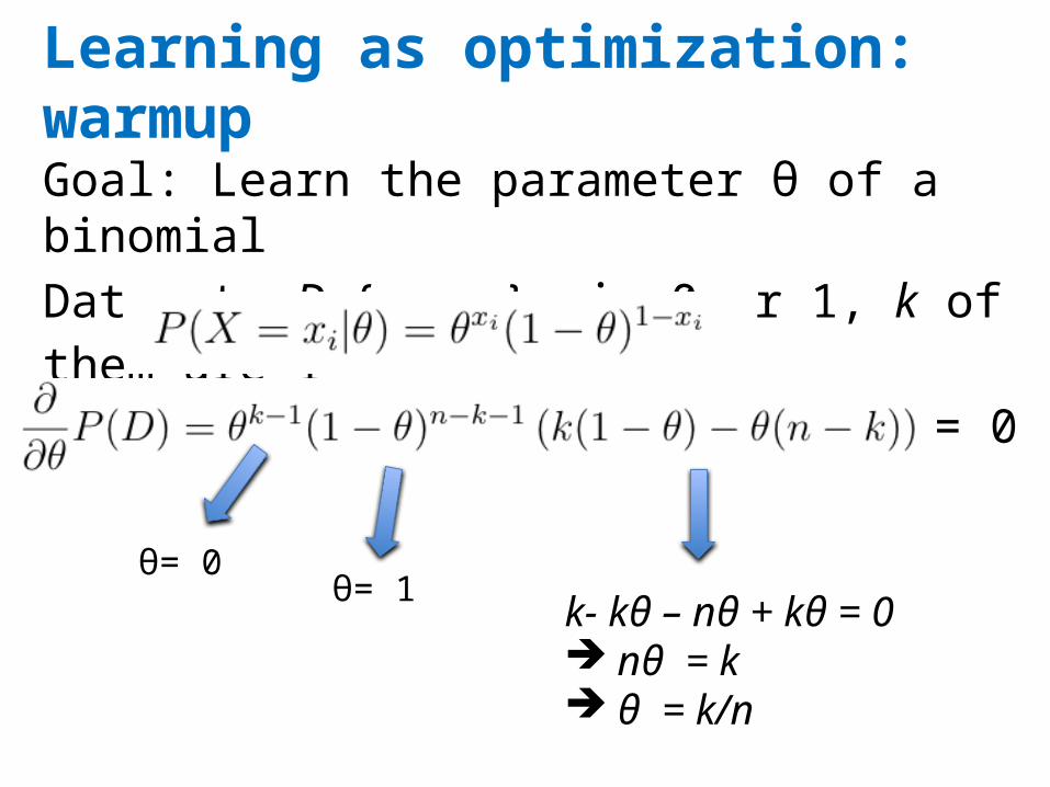
Learning as optimization: general procedure

• Goal: Learn the parameter θ of a classifier–probably θ is a vector

• Dataset: D={x1,…,xn}• Write down Pr(D|θ) as a function of θ• Maximize by differentiating and setting to zero

Learning as optimization: general procedure

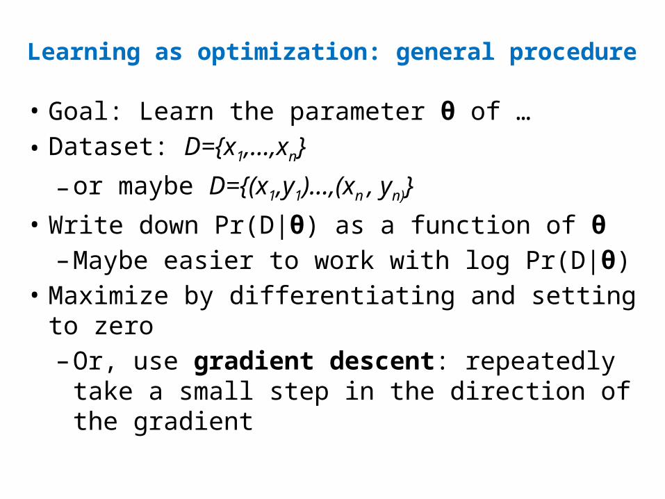
• Goal: Learn the parameter θ of …• Dataset: D={x1,…,xn}–or maybe D={(x1,y1)…,(xn , yn)}

• Write down Pr(D|θ) as a function of θ–Maybe easier to work with log Pr(D|θ)

• Maximize by differentiating and setting to zero–Or, use gradient descent: repeatedly take a small step in the direction of the gradient

Learning as optimization: general procedure for SGD

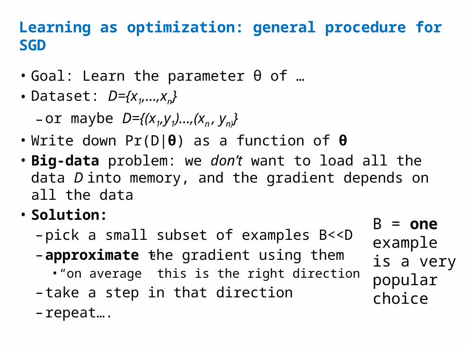
• Goal: Learn the parameter θ of …• Dataset: D={x1,…,xn}– or maybe D={(x1,y1)…,(xn , yn)}

• Write down Pr(D|θ) as a function of θ• Big-data problem: we don’t want to load all the data D into memory, and the gradient depends on all the data• Solution: – pick a small subset of examples B<<D– approximate the gradient using them

• “on average” this is the right direction– take a step in that direction– repeat….

B = one example is a very popular choice

Learning as optimization for logistic regression

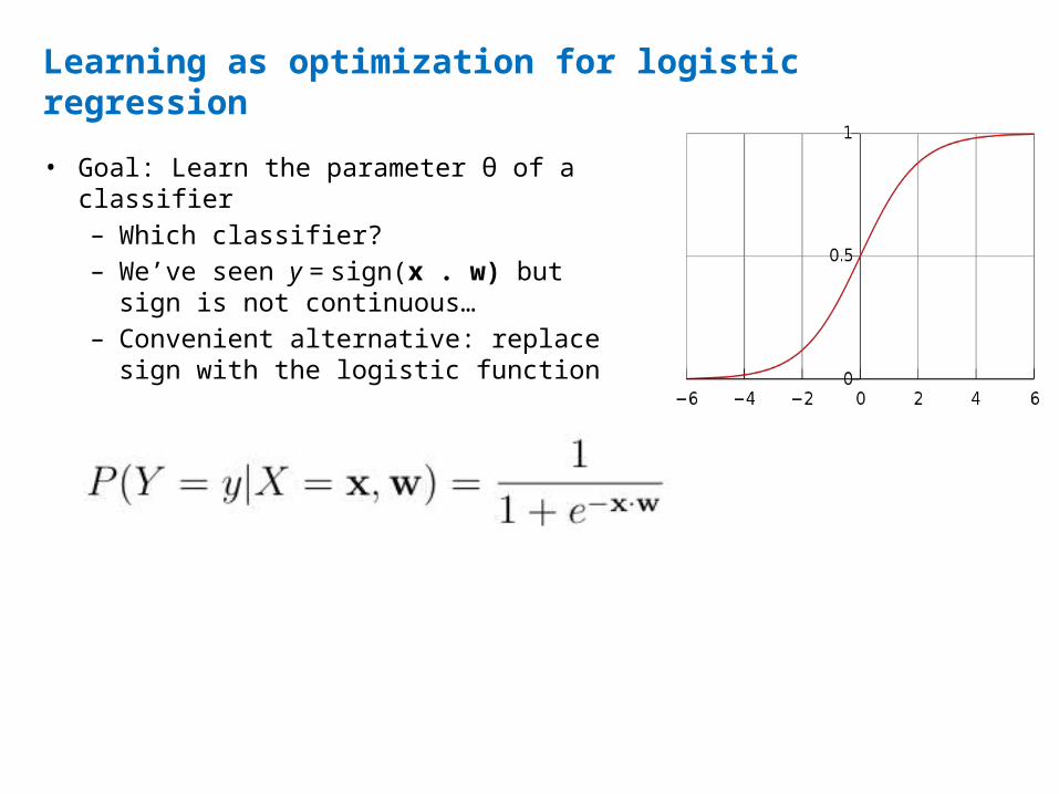
• Goal: Learn the parameter θ of a classifier– Which classifier?– We’ve seen y = sign(x . w) but sign is not continuous…– Convenient alternative: replace sign with the logistic function

Learning as optimization for logistic regression

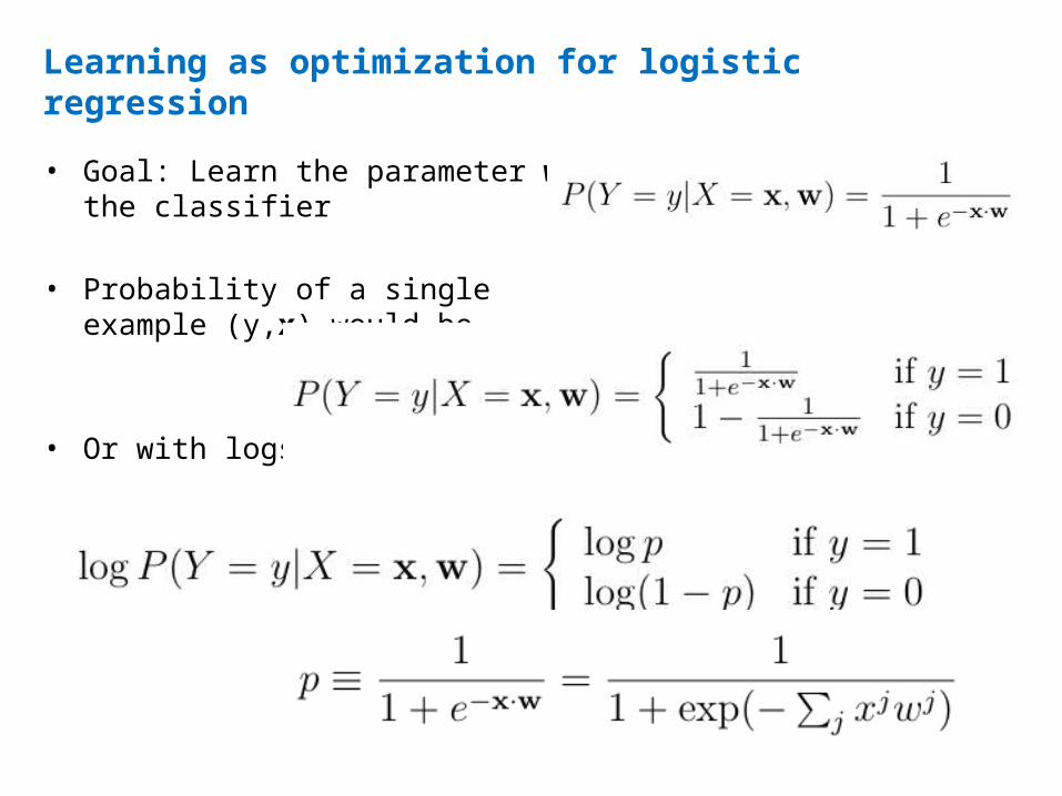
• Goal: Learn the parameter w of the classifier• Probability of a single example (y,x) would be• Or with logs:

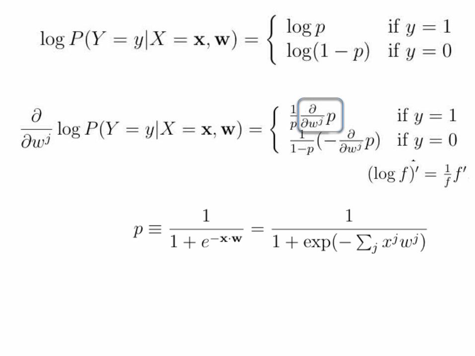
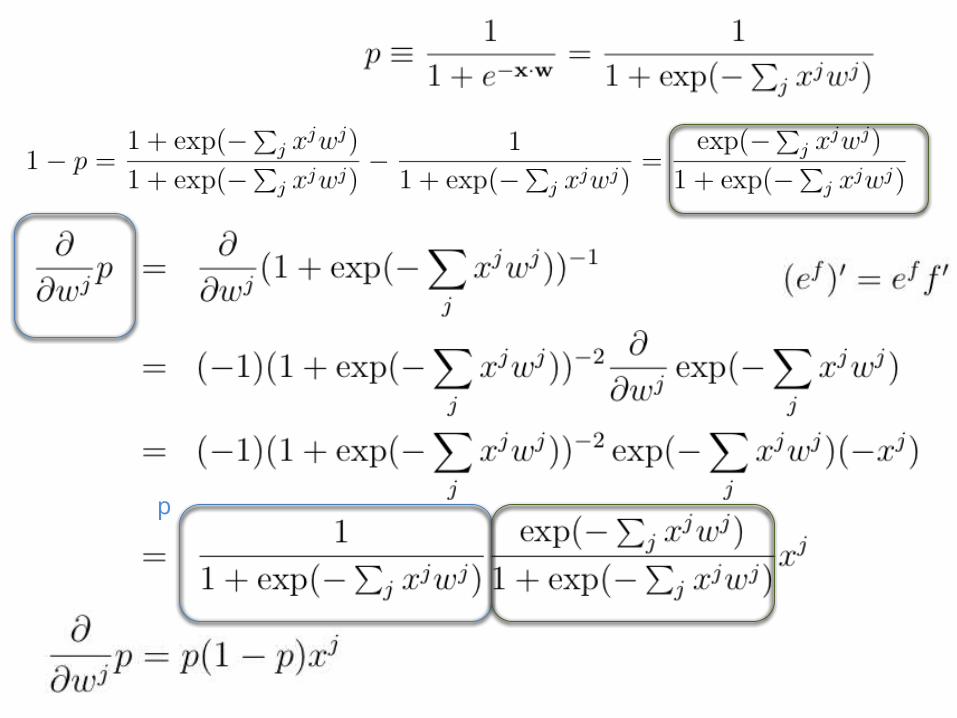
p

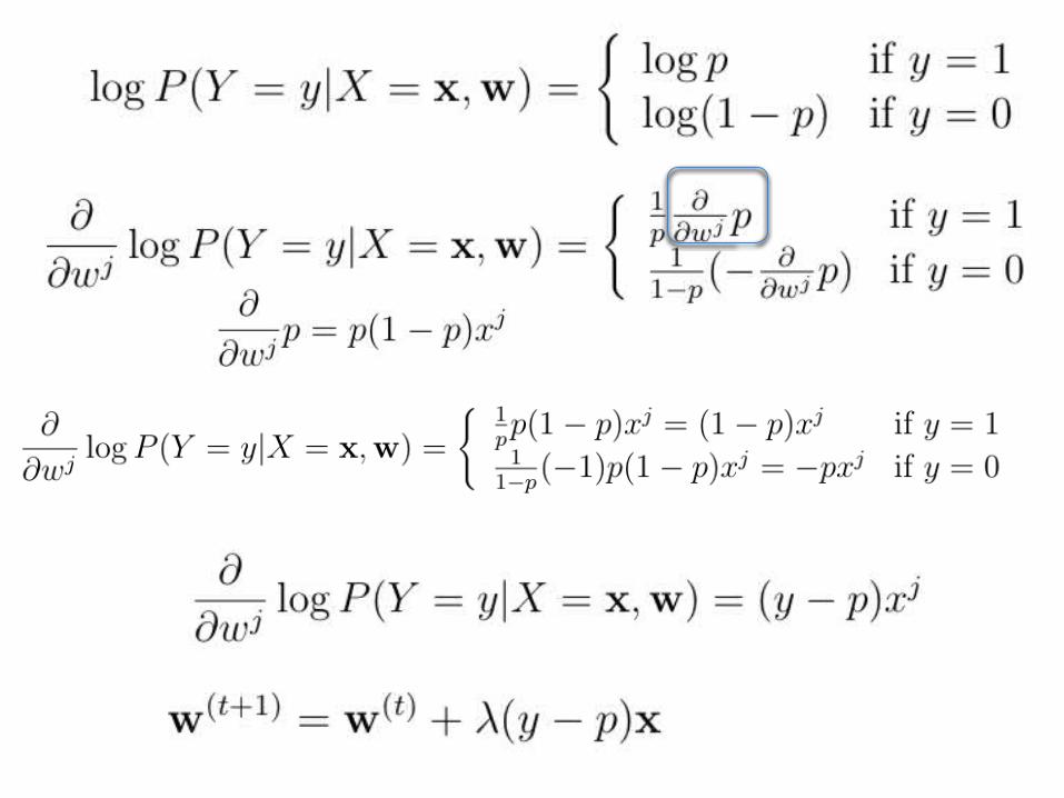
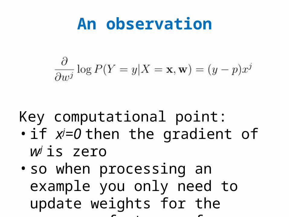
Key computational point: • if xj=0 then the gradient of wj is zero• so when processing an example you only need to update weights for the non-zero features of an example.

An observation

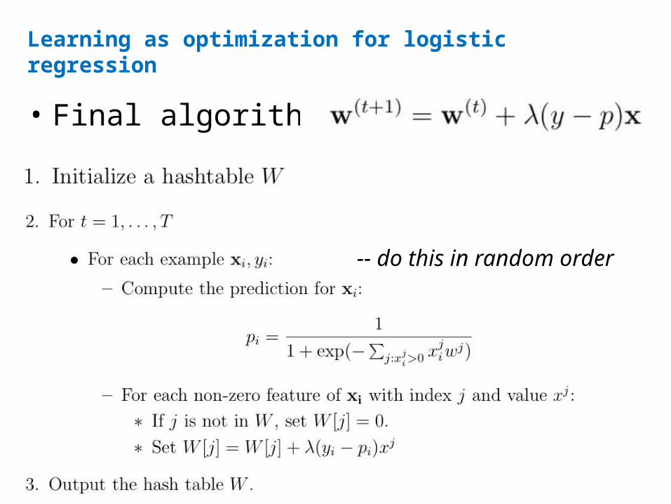
Learning as optimization for logistic regression

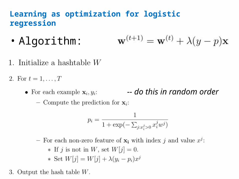
• Final algorithm:-- do this in random order

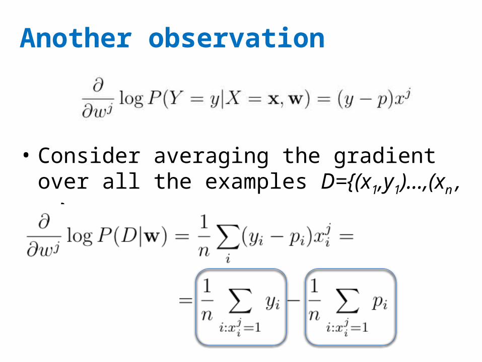
Another observation

• Consider averaging the gradient over all the examples D={(x1,y1)…,(xn , yn)}

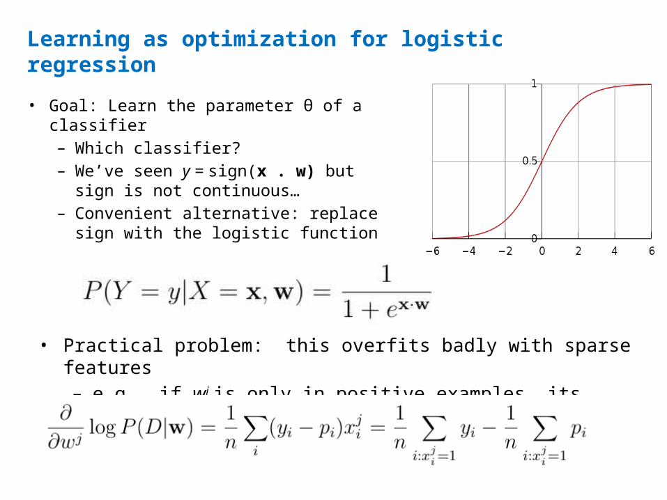
Learning as optimization for logistic regression

• Goal: Learn the parameter θ of a classifier– Which classifier?– We’ve seen y = sign(x . w) but sign is not continuous…– Convenient alternative: replace sign with the logistic function

• Practical problem: this overfits badly with sparse features– e.g., if wj is only in positive examples, its gradient is always positive !

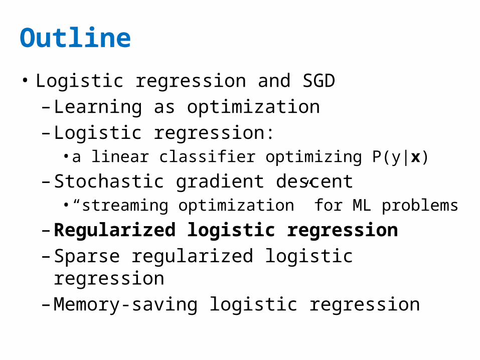
Outline

• Logistic regression and SGD–Learning as optimization–Logistic regression: • a linear classifier optimizing P(y|x)

–Stochastic gradient descent• “streaming optimization” for ML problems

–Regularized logistic regression–Sparse regularized logistic regression–Memory-saving logistic regression

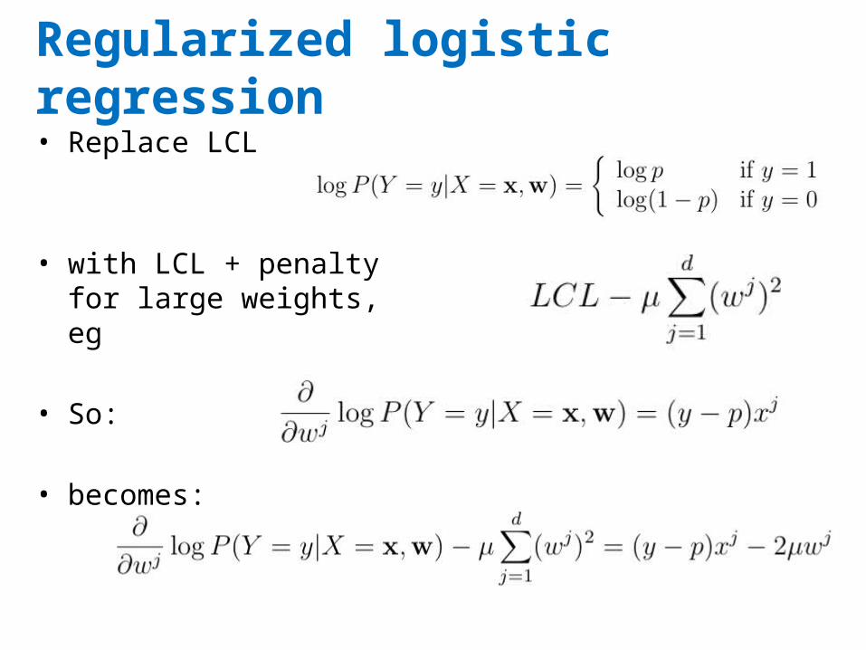
Regularized logistic regression• Replace LCL• with LCL + penalty for large weights, eg• So:• becomes:

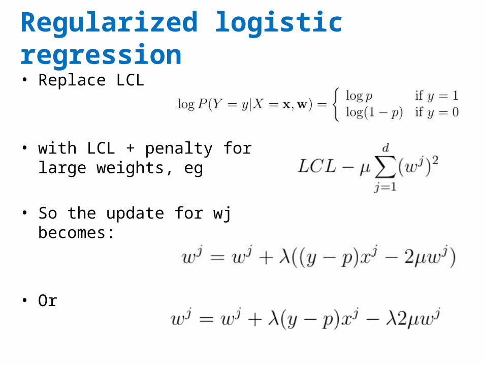
Regularized logistic regression• Replace LCL• with LCL + penalty for large weights, eg• So the update for wj becomes:• Or

Learning as optimization for logistic regression

• Algorithm:-- do this in random order

Learning as optimization for regularized logistic regression

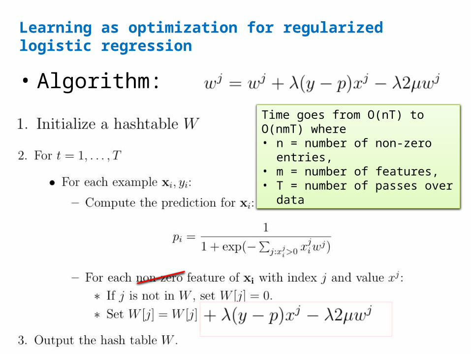
• Algorithm:Time goes from O(nT) to O(nmT) where• n = number of non-zero

entries, • m = number of features, • T = number of passes over

data

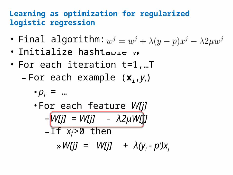
Learning as optimization for regularized logistic regression

• Final algorithm:• Initialize hashtable W• For each iteration t=1,…T– For each example (xi,yi)• pi = …• For each feature W[j]–W[j] = W[j] - λ2μW[j]–If xij>0 then»W[j] = W[j] + λ(yi - pi)xj

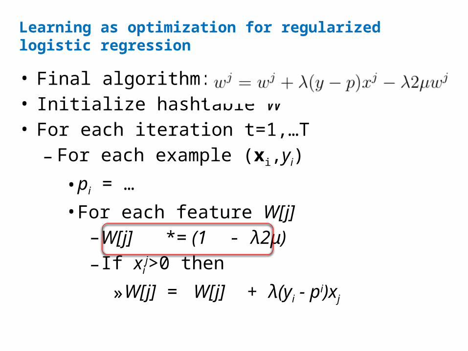
Learning as optimization for regularized logistic regression

• Final algorithm:• Initialize hashtable W• For each iteration t=1,…T– For each example (xi,yi)• pi = …• For each feature W[j]–W[j] *= (1 - λ2μ)–If xij>0 then»W[j] = W[j] + λ(yi - pi)xj

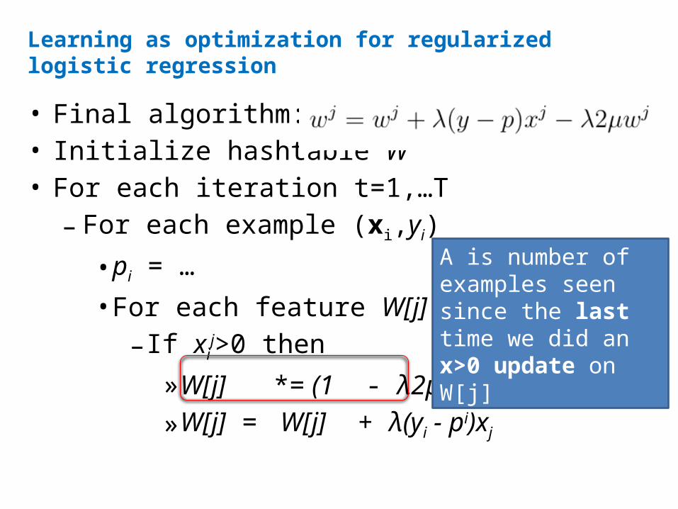
Learning as optimization for regularized logistic regression

• Final algorithm:• Initialize hashtable W• For each iteration t=1,…T– For each example (xi,yi)• pi = …• For each feature W[j]–If xij>0 then»W[j] *= (1 - λ2μ)A»W[j] = W[j] + λ(yi - pi)xj

A is number of examples seen since the last time we did an x>0 update on W[j]

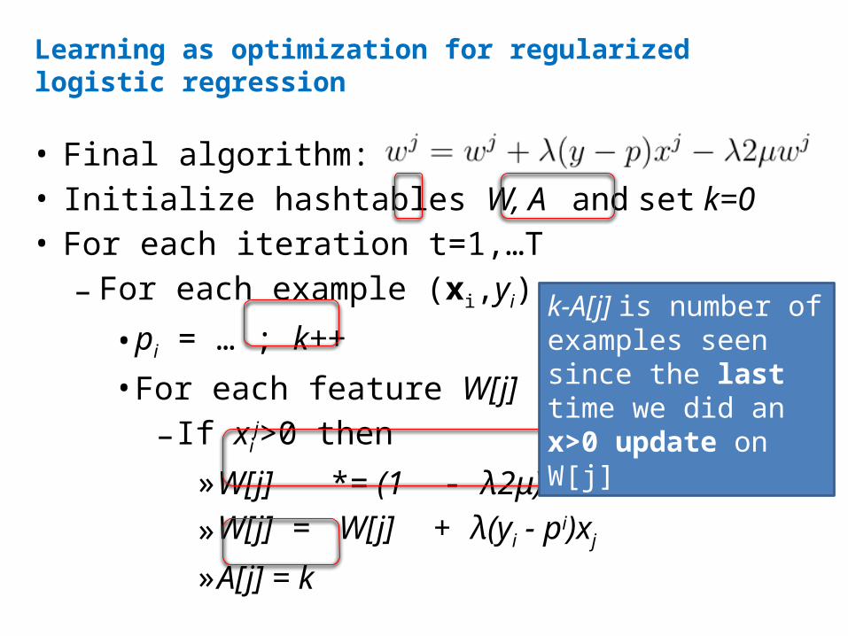
Learning as optimization for regularized logistic regression

• Final algorithm:• Initialize hashtables W, A and set k=0• For each iteration t=1,…T– For each example (xi,yi)• pi = … ; k++• For each feature W[j]–If xij>0 then»W[j] *= (1 - λ2μ)k-A[j]»W[j] = W[j] + λ(yi - pi)xj»A[j] = k

k-A[j] is number of examples seen since the last time we did an x>0 update on W[j]

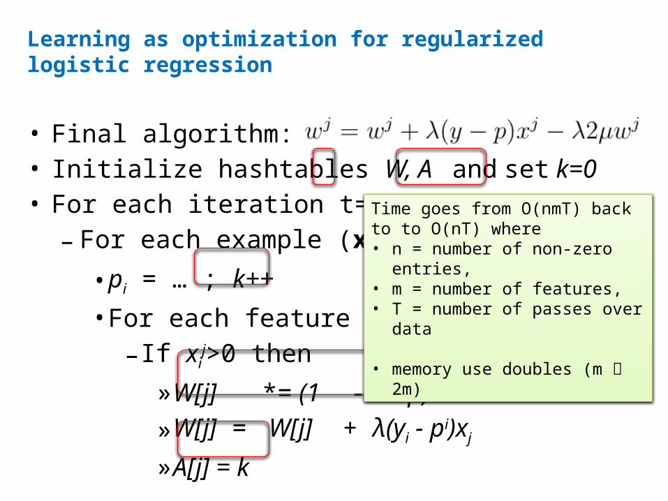
Learning as optimization for regularized logistic regression

• Final algorithm:• Initialize hashtables W, A and set k=0• For each iteration t=1,…T– For each example (xi,yi)• pi = … ; k++• For each feature W[j]–If xij>0 then»W[j] *= (1 - λ2μ)k-A[j]»W[j] = W[j] + λ(yi - pi)xj»A[j] = k

Time goes from O(nmT) back to to O(nT) where• n = number of non-zero

entries, • m = number of features, • T = number of passes over

data

• memory use doubles (m 2m)

Outline

• [other stuff]• Logistic regression and SGD– Learning as optimization– Logistic regression: • a linear classifier optimizing P(y|x)

– Stochastic gradient descent• “streaming optimization” for ML problems

–Regularized logistic regression– Sparse regularized logistic regression–Memory-saving logistic regression

Pop quiz

• In text classification most words area. rareb. not correlated with any classc. given low weights in the LR classifierd. unlikely to affect classificatione. not very interesting

Pop quiz

• In text classification most bigrams area. rareb. not correlated with any classc. given low weights in the LR classifierd. unlikely to affect classificatione. not very interesting

Pop quiz

• Most of the weights in a classifier are– important–not important

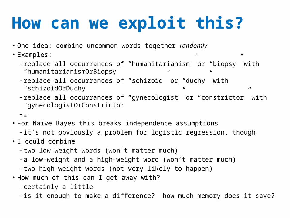
How can we exploit this?• One idea: combine uncommon words together randomly• Examples:

– replace all occurrances of “humanitarianism” or “biopsy” with “humanitarianismOrBiopsy”– replace all occurrances of “schizoid” or “duchy” with “schizoidOrDuchy”– replace all occurrances of “gynecologist” or “constrictor” with “gynecologistOrConstrictor”– …

• For Naïve Bayes this breaks independence assumptions– it’s not obviously a problem for logistic regression, though

• I could combine– two low-weight words (won’t matter much)– a low-weight and a high-weight word (won’t matter much)– two high-weight words (not very likely to happen)

• How much of this can I get away with?– certainly a little– is it enough to make a difference? how much memory does it save?

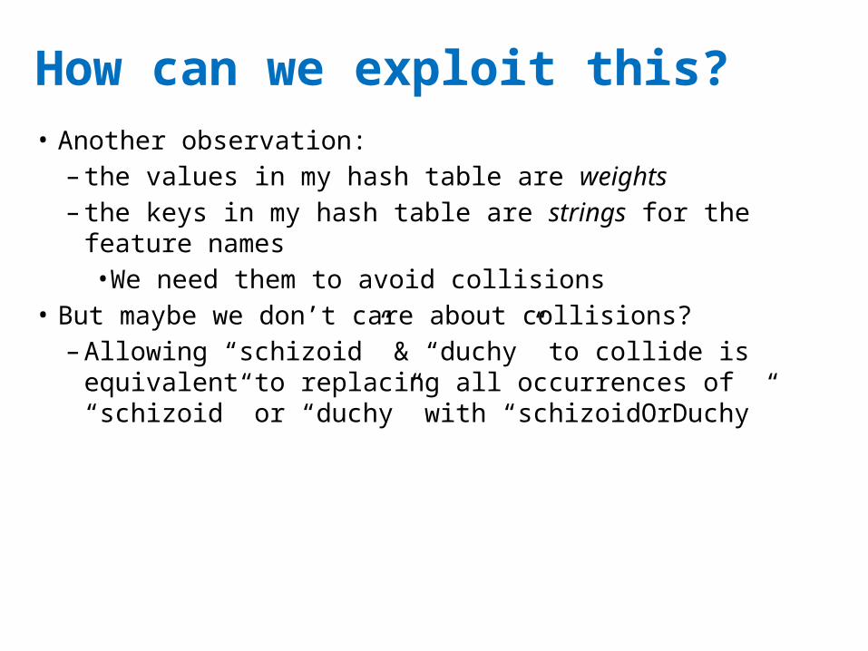
How can we exploit this?• Another observation: – the values in my hash table are weights– the keys in my hash table are strings for the feature names• We need them to avoid collisions

• But maybe we don’t care about collisions?– Allowing “schizoid” & “duchy” to collide is equivalent to replacing all occurrences of “schizoid” or “duchy” with “schizoidOrDuchy”

Learning as optimization for regularized logistic regression

• Algorithm:• Initialize hashtables W, A and set k=0• For each iteration t=1,…T– For each example (xi,yi)• pi = … ; k++• For each feature j: xij>0:

»W[j] *= (1 - λ2μ)k-A[j]»W[j] = W[j] + λ(yi - pi)xj»A[j] = k

Learning as optimization for regularized logistic regression

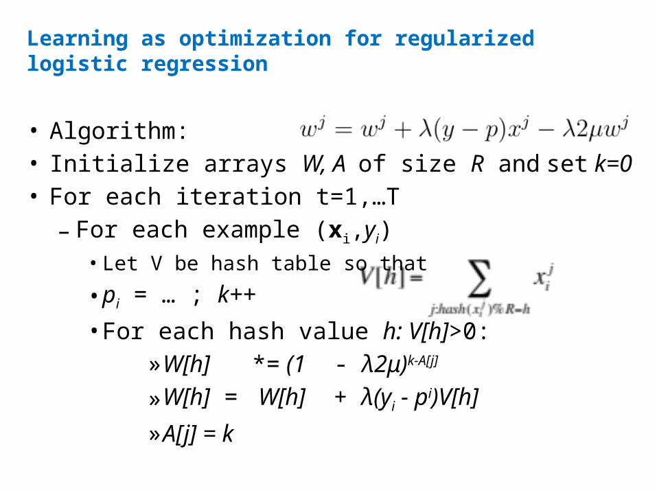
• Algorithm:• Initialize arrays W, A of size R and set k=0• For each iteration t=1,…T– For each example (xi,yi)• Let V be hash table so that • pi = … ; k++• For each hash value h: V[h]>0:

»W[h] *= (1 - λ2μ)k-A[j]»W[h] = W[h] + λ(yi - pi)V[h]»A[j] = k

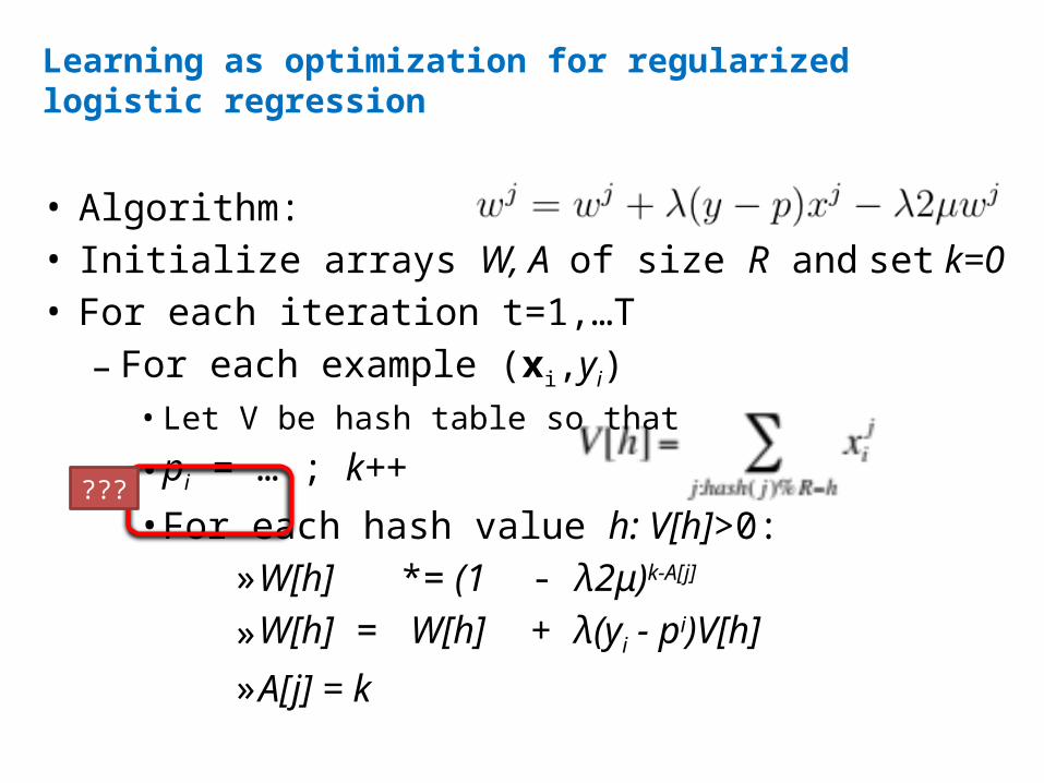
Learning as optimization for regularized logistic regression

• Algorithm:• Initialize arrays W, A of size R and set k=0• For each iteration t=1,…T– For each example (xi,yi)• Let V be hash table so that • pi = … ; k++• For each hash value h: V[h]>0:

»W[h] *= (1 - λ2μ)k-A[j]»W[h] = W[h] + λ(yi - pi)V[h]»A[j] = k

???

ICML 2009

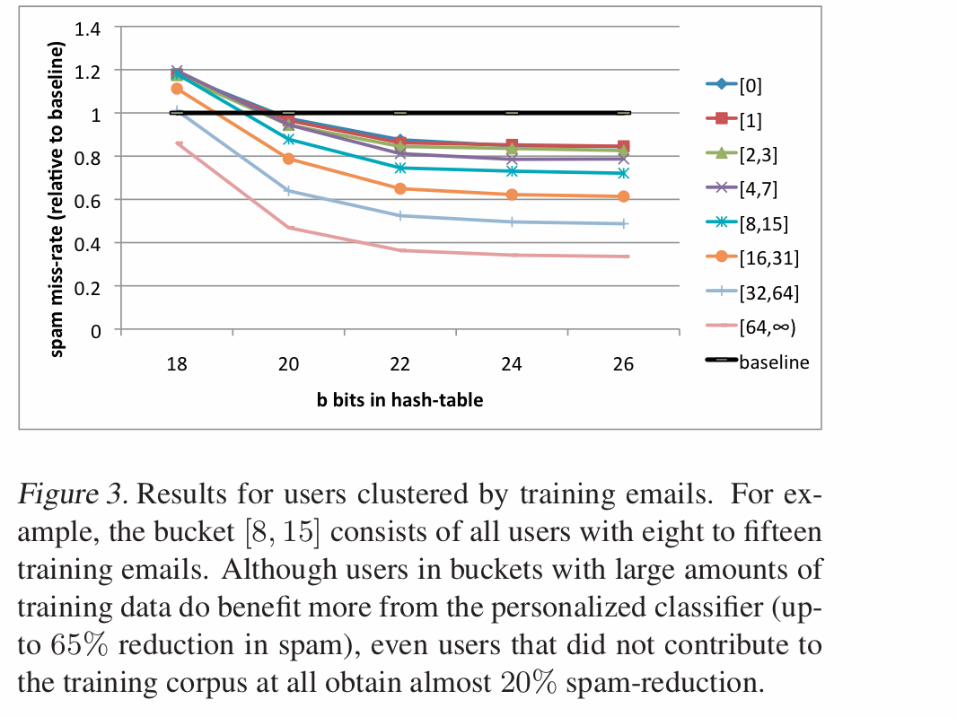
An interesting example• Spam filtering for Yahoo mail– Lots of examples and lots of users– Two options:• one filter for everyone—but users disagree• one filter for each user—but some users are lazy and don’t label anything

– Third option:• classify (msg,user) pairs• features of message i are words wi,1,…,wi,ki• feature of user is his/her id u• features of pair are: wi,1,…,wi,ki and uwi,1,…,uwi,ki • based on an idea by Hal Daumé

An example

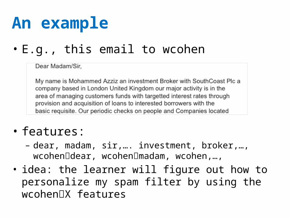
• E.g., this email to wcohen

• features:– dear, madam, sir,…. investment, broker,…, wcohendear, wcohenmadam, wcohen,…,

• idea: the learner will figure out how to personalize my spam filter by using the wcohenX features

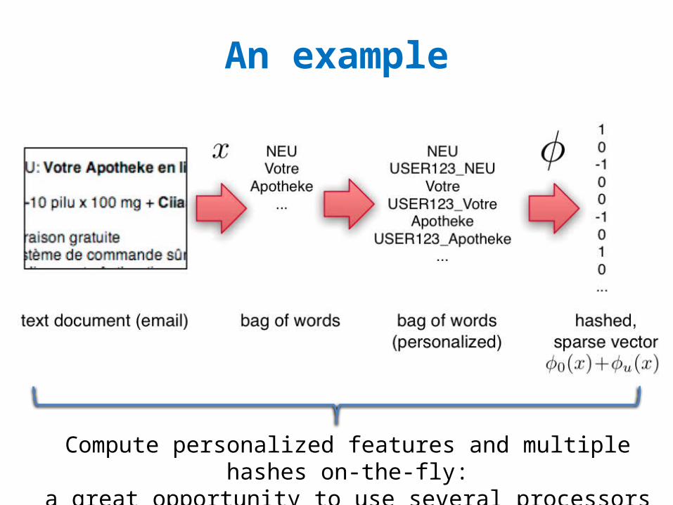
An example

Compute personalized features and multiple hashes on-the-fly:

a great opportunity to use several processors and speed up i/o

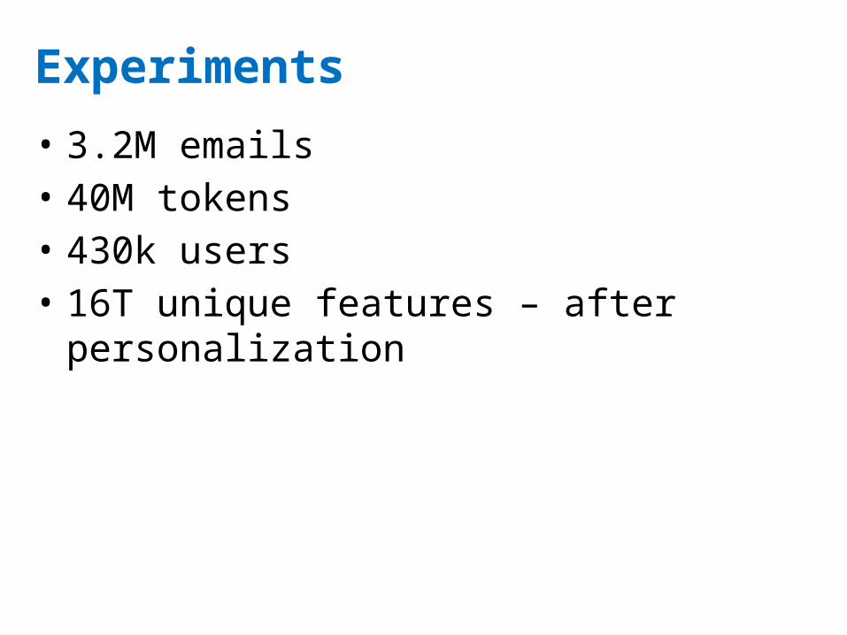
Experiments

• 3.2M emails• 40M tokens• 430k users• 16T unique features – after personalization

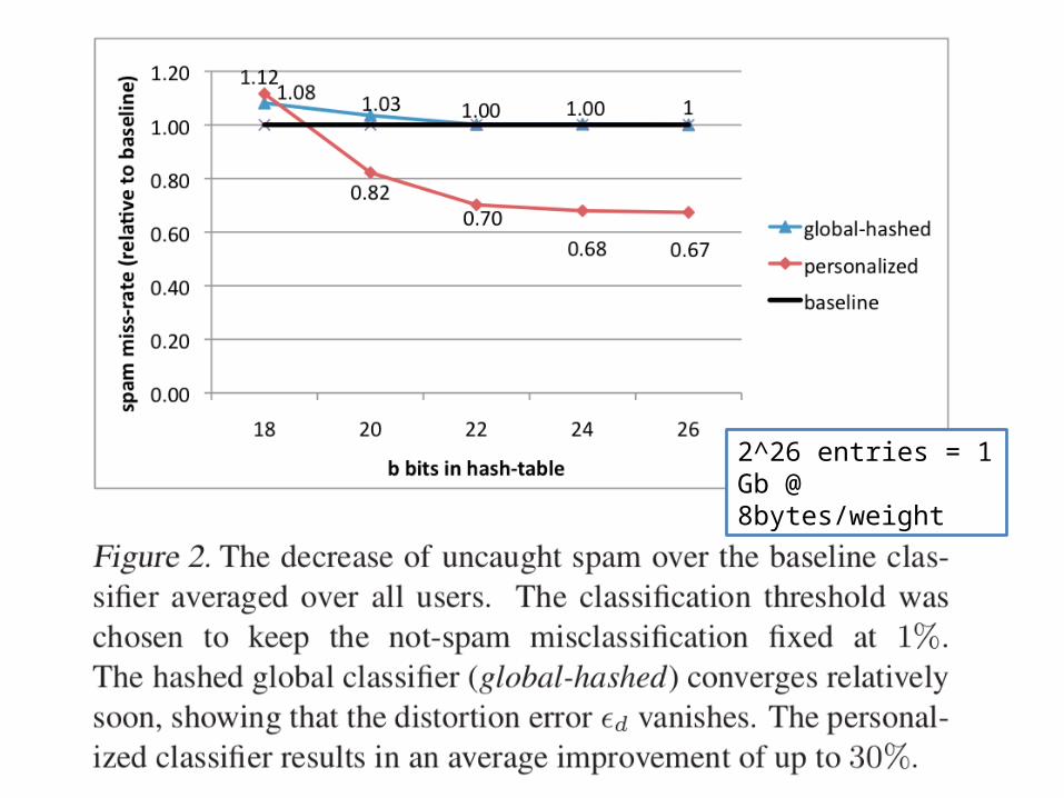
An example

2^26 entries = 1 Gb @ 8bytes/weight