
Robson Valley Enhanced Forest Management Pilot Project ... · Robson Valley Enhanced Forest...
71
0 Robson Valley Enhanced Forest Management Pilot Project Coarse Woody Debris Assessment Phase ΙII (A comparative assessment of coarse woody debris volume and wildlife habitat quality in clearcut silviculture systems using groundbased harvesting methods under pre and postharvest conditions) Final Report Prepared for Chris Ritchie BC Ministry of Water, Land and Air Protection 325, 1011 Fourth Avenue Prince George, BC, V2L 3H9 Prepared by Bruce Rogers, B.Sc., Wildlife Biologist 1355 LaSalle Avenue Prince George, BC V2L 4K1 250-561-1792 February 2002
Transcript of Robson Valley Enhanced Forest Management Pilot Project ... · Robson Valley Enhanced Forest...

0
Robson Valley Enhanced Forest Management Pilot Project Coarse Woody Debris Assessment Phase ΙII
(A comparative assessment of coarse woody debris volume and wildlife habitat quality in clearcut silviculture systems using groundbased harvesting methods under pre and
postharvest conditions)
Final Report
Prepared for Chris Ritchie BC Ministry of Water, Land and Air Protection
325, 1011 Fourth Avenue Prince George, BC, V2L 3H9
Prepared by Bruce Rogers, B.Sc., Wildlife Biologist 1355 LaSalle Avenue Prince George, BC
V2L 4K1 250-561-1792
February 2002

1
Contents Summary ............................................................................................................................................3 Introduction........................................................................................................................................3 Study Background..............................................................................................................................4 Objectives ..........................................................................................................................................4 Information Gaps ...............................................................................................................................5 Methods..............................................................................................................................................7 • Site selection and rationale ..........................................................................................................7 • Study sites ....................................................................................................................................8 • Plot location and establishment procedures.................................................................................8 • CWD sampling procedures ..........................................................................................................8 • Data Analysis ...............................................................................................................................8 Results................................................................................................................................................9 • Mean volume ...............................................................................................................................9 • Mean Decay Class........................................................................................................................11 • Mean Wildlife Types ...................................................................................................................13 • Mean Number Wildlife Types per piece......................................................................................15 • Per Cent tree species with 1 or more Wildlife Type....................................................................16 • Mean Number Wildlife Types per class ......................................................................................17 Discussion/Recommendations ...........................................................................................................19 • Discussion of sampling variables.................................................................................................21 • Recommendations........................................................................................................................26 Literature Cited ..................................................................................................................................29 Tables Table 1. District subzones, proposed subzones for harvest, and subzones with CWD information 6 Table 2. Percent proposed harvest method application in the Robson Valley Forest District..........7 Tables 3-7. Results of testing the hypothesis of no difference between TU and UN........................10 Tables 8-10. Comparative results (Northern Wetbelt and EFMPP studies) ....................................21 Figures Figures 1-21. Graphs for all sampling variables...............................................................................11
Appendix
Appendix 1 Study sites chosen for 2001 CWD survey......................................................................32 Appendix 2: Mean Values of variables..............................................................................................33 Appendix 3: CWD Decay Classes .....................................................................................................39 Appendix 4; CWD Wildlife Types ....................................................................................................40 Appendix 5-10: Full statistical output for all sampling variables......................................................41

2
Acknowledgments The author would like to acknowledge the following individuals for their assistance: Susan Stevenson (Silvifauna Research) for editing and input on study rationale; Steve Day (Slocan Forest Products Ltd.), Mike Jackman (McBride Forest Industry Ltd.), and Greg Clements (Robson Valley Forest District) for providing site information; Craig DeLong (BC Ministry of Forests), Aled Hoggett (UBC Forestry Department); Susan Hoyles (BC Ministry of Forests), and Mike Jull and Susan Stevenson (Northern Wetbelt Silviculture Systems Project, UNBC), for supplying information regarding Coarse Woody Debris surveys that have been conducted in the study area to date. Dieter Ayres of UNBC supplied statistical analysis. Fieldwork was done by E.P. Runtz and Associates of McBride B.C. Summary In the fall of 2002 a Coarse Woody Debris (CWD) survey was conducted in the Robson Valley Forest District for the Enhanced Forest Management Pilot Project (EFMPP) as a pilot study. Data were collected to determine levels of volume, decay class, and wildlife habitat types found in clearcut versus unharvested areas across biogeoclimatic subzones located in this forest district. Prior to this, information gaps were determined for ecosystems that lacked information on CWD. Allotment of proposed harvest along with utilization of silviculture systems and harvesting methods were also summarized. Out of 12 biogeoclimatic subzones proposed for harvest, the Engelmann spruce-subalpine fir zone comprises 44.5 % of the harvest. This is considerable in relation to the other subzones. Only 2 subzones, the ESSFwk2 and ICHwk3, were found to have information on CWD. Based on information gathered from The Robson Valley Forest District Small Business Forest Enterprise Program, McBride Forest Industry, and Slocan Forest Products forest development plans, clearcut or clearcut with reserves comprised 85% of the silviculture systems used in the valley, while ground based harvesting methods were used in 54% of the silviculture prescriptions that were reviewed. This knowledge formed the basis for site selection. Data analysis revealed the following general trends for CWD where groundbased harvesting methods were used in clearcut silviculture systems:
• No significant difference was detected for volume between the clearcut and unharvested units;
• The presence of Decay Class 1 and 2 appears to be higher in the harvested units. This harvesting method may reduce the presence of Decay Class 4 and 5 pieces, along with wildlife habitat Types 1, 3, and 5;
• In the ESSF subzones there was a significant increase in the number of subalpine fir pieces found in the clearcuts over that of the unharvested units;
• In the harvested units, early Decay Classes appear by observation to have more types associated with them than later Decay Classes. Later Decay Classes may be more prone to losing types through destruction or having them covered up by slash
Implications and recommendations based on these findings are discussed at the end of this report.
Introduction In recent years forest managers have become increasingly aware of the role of trees with special characteristics and of fallen woody material in maintaining biodiversity. They have realized that these forest elements, which often result from damage or disease, provide critical wildlife habitat that will not necessarily be available in managed stands unless special measures are taken to insure their presence. In British Columbia, several initiatives have been taken to provide wildlife trees and coarse woody debris (CWD) in managed stands. In the Biodiversity Guide Book (1995), B.C. Ministry of Forests and B.C. Ministry of Environment Lands and Parks recommend how the retention of those structures should be integrated into forest management at the landscape and stand levels. Through a series of decay stages, standing trees eventually become non-self supporting and fall to the ground, subsequently becoming CWD. Trees and stumps that are still intact and in the ground are still considered self supporting, and are thus not considered CWD (Resource Inventory Committee, 1997, not seen; cited by Buckland et al. 1998). CWD provides potential habitat by creating nest sites, dens, and security cover for small mammals and birds. It provides ground level and elevated runways across streams, along the forest floor and up into the canopy. It is also an important source of moist microsites for amphibians, insects, plants and ectomycorrhizal fungi (O’neil et al. 1997, not seen; cited by Buckland et al. 1998). Hollow logs, created by heartwood fungi when the tree was standing are important as cover or denning sites for a variety of large mammals, including snowshoe hares, bushy tailed woodrats, weasels, skunks and black bears (Akenson and Henjum 1994, Maser et al. 1979, not seen; cited by Jull et al. 2000). Some animals such as red squirrels, cache winter food supplies in hollow logs (Maser et al. 1979, not seen; cited by Jull et al. 2000). The root wad of uprooted trees is an important habitat feature that is used by flycatchers for perching, by grouse for dusting, by juncos for nesting and by winter wrens for both foraging and nesting (Campbell et al. 1997, not seen; cited by Jull et al. 2000). However, other factors, such as size, decay stage, orientation and quantity of CWD have a greater influence than mode of death on how the fallen trees are used by wildlife (Caza 1993, not seen; cited by Jull et al. 2000). This survey provides quantitative information about the structural habitat features provided by CWD in the Robson Valley Enhanced Forest Management Pilot Project (EFMPP) area. It was conducted within the Robson Valley Forest District boundary. The Robson Valley Forest District and local licensees Slocan Forest Products Ltd. and McBride Forest Industry Ltd. have facilitated this project with the appropriate site history and site access information. Study Background This project is composed of 3 phases. The goal of Phase 1 for the EFMPP CWD survey was to identify information gaps, and to provide those carrying out the 2001 field sampling with site locations and current sampling methodology. This information defines the basis and rationale for Phase 2 (data collection). Phase 3 is the report and recommendations, and will help guide direction of future study of CWD in the Robson Valley Forest District.
3

4
The EFMPP requires information regarding CWD volume and wildlife habitat attributes in relation to the predominant harvesting methods and silviculture systems used within the biogeoclimatic subzones of the project area. CWD data meeting current protocol (volume, decay class, and wildlife habitat attributes) were collected in representative harvested areas and adjacent unharvested areas. Objectives The objective of this project is to determine the levels of volume, wildlife habitat attributes, and decay class for CWD in harvested and unharvested areas. The ultimate goal is to collect and present data from harvested and unharvested areas representative of the levels of CWD found in the subzone variants that occur within this district. However, this pilot project is limited in budget, and has gathered data on CWD levels only in the subzones that have undergone and are proposed to undergo the highest levels of harvesting. The specific objectives of the pilot project are: • To identify biogeoclimatic subzones in the Robson Valley Forest District in which CWD
assessments have been done, and to provide a brief descriptive summary of this work (information gaps).
• To locate ecologically representative study sites that have been recently logged, and to
collect data based on the most recent CWD protocol used in the study area. • To compare the amount of CWD found in harvested and unharvested areas in the suzones
sampled. • To compare the wildlife habitat quality of CWD found in harvested and unharvested areas in
the subzones sampled. • To provide recommendations for further study of CWD within these subzones as it pertains
to wildlife habitat. Information gaps A gap analysis was conducted to determine the history of CWD surveys that have been conducted in the biogeoclimatic subzones of the Robson Valley Forest District (B.C. Ministry of Forests 1996). Based on this survey, it is clear that data on CWD are limited. Current information on CWD in the Robson Valley Forest District EFMPP is as follows: • In 1999 and 2000 the Northern Wet-belt ICH/ESSF Silviculture Systems Project Phase III
conducted CWD surveys in the ICHwk3 subzone. These surveys were carried out according to the CWD inventory methodology of the Resource Inventory Committee (1997) Ground Sampling Procedures. The wildlife habitat classification was based on an earlier draft of Keisker (2001). In this trial, ground based and cable harvesting systems were used, along with variable retention and clearcut silviculture systems. The East Twin and Minnow Creek

5
study sites are located approximately 35 km northwest of McBride BC, and were sampled extensively. The East Twin site has been sampled for pre-harvest and post-harvest CWD. The Minnow Creek site has been sampled for pre-harvest CWD and post-harvest measurements by the Northern Wet-belt field crew in 2001. (For details refer to Jull et al 1999). The results of the post harvest measurements are presently being analyzed.
• In 1999 the British Columbia Conservation Foundation carried out CWD surveys in the
ICHwk3 and ESSFwk2 subzones for the Robson Valley EFMPP. Transects of 100 m in length were established to sample old growth features. For each 100 m transect, a 30-m segment was randomly selected to measure CWD. For each piece greater than 7.5 cm in diameter at the point of interception, diameter was measured and decay class (according to Maser et al 1979) and CWD Wildlife Types according to an earlier draft of Keisker (2001) were assessed. Total volume of CWD for each plot was calculated using the formula described in Lofroth (1992), not seen, cited by Harrison et al. 2000.
• A study of Western Hemlock Looper and Forest Disturbance in the ICHwk3 of the Robson
Valley was conducted by a Ph.D. candidate from the University of British Columbia in 2000. In this study CWD was defined as any dead stem that formed an angle of less than 45 degrees with the ground, and was greater than 10cm average diameter where it was intersected by the transect line. CWD was classified using a decay class system based on that of Triska and Cromack (1980, not seen, cited by Hogget 2000). A class was added to the classification to allow differentiation between heavily decayed CWD found on the forest floor (Class 5), and heavily decayed CWD that was largely submerged within the forest floor (Class 6) (Hogget 2000).
• In 1997, as part of the Treatment Regime Evaluation Numerical Decision Support
(TRENDS) program of the Northern Interior Vegetation Management Association (NIVMA), nine CWD plots were installed and measured for volume and decay class according to Resource Inventory Committee ground sampling protocol (Resource Inventory Committee 1997). Six of the plots are in the ICHwk3, and three are in the ESSFmm1. Six of the plots were re-measured in 2000 for post-harvest CWD. The data can be accessed from the Prince George Region NIVMA Data Base (Industrial Forestry Services Ltd.) (Hoyles S. pers. com., 2001)
• Waste management surveys have also been conducted by licensees to determine the levels of
felled timber and slash remaining on cutblocks after harvesting. The objectives of these surveys are to meet license obligations and are not ecologically based.
The ICHwk3 and ESSFwk2 are the only subzones that have been sampled using the desired data collection protocol of the Robson Valley EFMPP. Jull et al. (2000) and Harrison et al. (2000) used the most recently developed CWD habitat assessment methodology. Jull et al. (2000) was the only study to use variable retention treatment with a pre and post-harvest experimental design, although Hoyles (2001) also sampled pre and post-harvest plots.
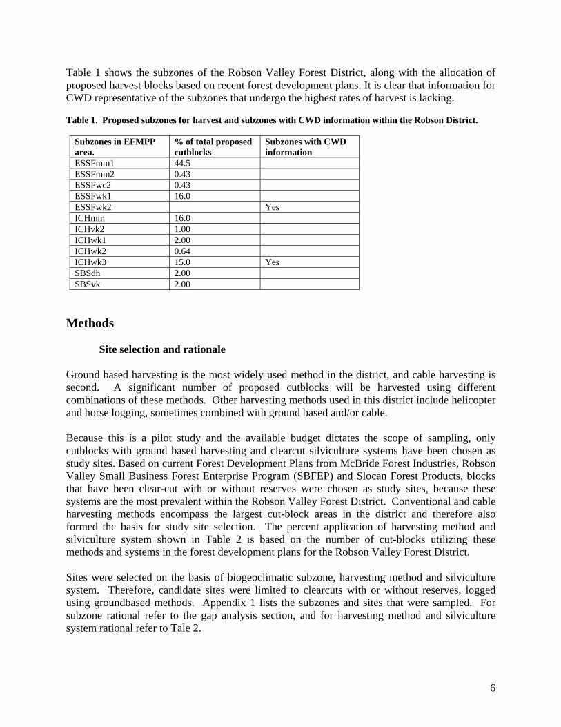
Table 1 shows the subzones of the Robson Valley Forest District, along with the allocation of proposed harvest blocks based on recent forest development plans. It is clear that information for CWD representative of the subzones that undergo the highest rates of harvest is lacking. Table 1. Proposed subzones for harvest and subzones with CWD information within the Robson District.
Subzones in EFMPP area.
% of total proposed cutblocks
Subzones with CWD information
ESSFmm1 44.5 ESSFmm2 0.43 ESSFwc2 0.43 ESSFwk1 16.0 ESSFwk2 Yes ICHmm 16.0 ICHvk2 1.00 ICHwk1 2.00 ICHwk2 0.64 ICHwk3 15.0 Yes SBSdh 2.00 SBSvk 2.00
Methods
Site selection and rationale Ground based harvesting is the most widely used method in the district, and cable harvesting is second. A significant number of proposed cutblocks will be harvested using different combinations of these methods. Other harvesting methods used in this district include helicopter and horse logging, sometimes combined with ground based and/or cable. Because this is a pilot study and the available budget dictates the scope of sampling, only cutblocks with ground based harvesting and clearcut silviculture systems have been chosen as study sites. Based on current Forest Development Plans from McBride Forest Industries, Robson Valley Small Business Forest Enterprise Program (SBFEP) and Slocan Forest Products, blocks that have been clear-cut with or without reserves were chosen as study sites, because these systems are the most prevalent within the Robson Valley Forest District. Conventional and cable harvesting methods encompass the largest cut-block areas in the district and therefore also formed the basis for study site selection. The percent application of harvesting method and silviculture system shown in Table 2 is based on the number of cut-blocks utilizing these methods and systems in the forest development plans for the Robson Valley Forest District. Sites were selected on the basis of biogeoclimatic subzone, harvesting method and silviculture system. Therefore, candidate sites were limited to clearcuts with or without reserves, logged using groundbased methods. Appendix 1 lists the subzones and sites that were sampled. For subzone rational refer to the gap analysis section, and for harvesting method and silviculture system rational refer to Tale 2.
6

Within the Robson Valley Forest District, 11 Biogeoclimatic Subzones were identified as ecosystems lacking any information on Coarse Woody Debris. Subzones where information exists, and the related methodology is mentioned in the Information Gaps section. Table 2: Percent proposed application of Ground Based (GB), Cable/Ground Based (C/GB), Cable (C)
harvesting methods, Clear-cut (CC)/Clear-cut-reserves (CCR) silviculture systems, and other (helicopter and horse logging and all methods combined) in the Robson Valley Forest District, based on the current forest development plans.
Harvesting method/Silviculture system
% harvesting method used in district
% silviculture systems used in district
GB 34 C/GB 20 C 16 CC/CCR 85 other 30 15
Study sites
Candidate cutblocks were provided by local licensees and the forest district, and were plotted throughout the study range on a 1:20,000 scale grid over lay of the Robson Valley Forest District. Silviculture prescriptions with hemlock looper salvage were removed.
Plot location and establishment procedures Areas that were harvested using ground based harvesting methods have been chosen for this study. Although some blocks selected for the study include portions that were cable-logged, sampling was restricted to the areas where the harvesting was ground based. A portion of the block edge that met establishment criteria (described in Rogers 2001) and was accessible was chosen, with the tie point located at a randomly chosen point along the edge portion. When locating plot establishment points the following site features were avoided, as these site characteristics may represent inordinate levels of CWD input.
-draws, gullies, and creek beds -extreme slopes -bog, marsh or fen -forest that has been logged or disturbed beyond the cutblock harvest boundary Paired plots were established in each cut-block. One in the clearcut and one in the unharvested area adjacent to the block edge. Lines perpendicular to the block edge were run for 100 m into the block and into the unharvested area. One transect 24 m in length was established on a random bearing. A coin toss determined which perpendicular direction another 50 m line was run. At that end point another transect was established. Returning to the point of commencement of the first transect a 50 m line was then walked back along the original line, where the third transect was then established. This procedure was repeated in both the harvested treatment unit (TU) and unharvested (UN) areas.
7

CWD sampling procedures
CWD decay class and volume data were collected as per the Resource Inventory Committee 1997, and CWD Wildlife Types Data was collected consistently with that of the Northern Wetbelt Silviculture Systems Project using Kiesker 2001.
Data Analysis
Volume calculations CWD volume was calculated according to Van Wagner (1982). Odd shaped pieces were calculated as per Marshall (1999). These formulas were also used to calculate CWD volume in Jull et al. 2001. The formulas used were as follows: V = (1.234/L) (d2 x a) where V is volume in m3 /ha, L is transect length (m), d is piece diameter in cm at the point of intersection with the sample line, and a is the secant of the tilt angle (away from the horizontal) of each piece sampled. Odd shaped pieces V = W x H/L x 10,000 m2/ha where V is the volume (m3 /ha) represented by an odd shaped piece crossed by the line transect, W is the width (m) of the rectangle associated with the odd-shaped piece, as measured along the length of the line transect, H is the effective height (m) of the odd-shaped piece, and L is the length (m) of the line transect. Statistical analysis Analysis was carried out using R version 1.4.1 (Copyright 2002, The R Development Core Team). The primary issue with regards to the data is the sample size. A total of 18 plots were sampled, and these were spread out over 7 Subzones. There were 6 replications of the treatment in ESSFmm1, 3 in ESSFwk1, 2 in ICHwk3, 2 in ICHwk3/SBSvk, 3 in SBSvk, and one in each of ICHmm1 and SBSdh. Statistical analysis on the ICHmm1 and SBSdh subzones were not performed, because of the lack of replication in these subzones. Similarly, though statistical analysis can be carried out on the Subzones with 2 replications, the results from these analysis are rather suspect, and are not presented in the text. For this reason, only results from the ESSFmm1, ESSFwk1, and SBSdh are presented. Even these should be viewed with caution, due to the small sample sizes.
8

The statistical analysis of the data consisted of a number of paired sample t-tests. T-tests on approximately 25 dependent variables were carried out for each subzone. The data was visually examined to assess normality. Variable means by subzone can bee seen in Appendix 8, and statistical analysis output is listed in Appendix 3-7. Results
Analysis A: Mean Volume
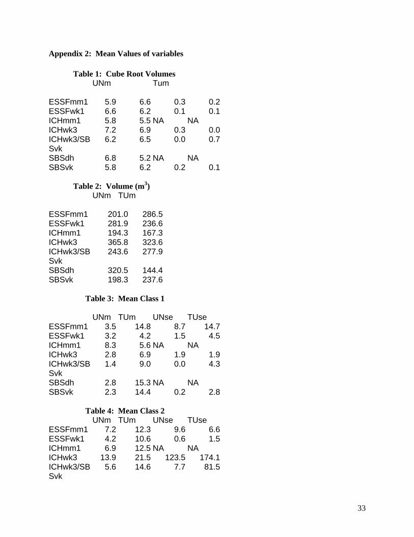
Volume analysis for this study showed no significant differences between clearcut treatment unit (TU) and the unharvested unit (UN) for any subzone. However, the ESSFmm1 did approach significance for the hypothesis; Differences do exist between the harvested and unharvested units. The mean volume of the coarse woody debris was compared across the treated and untreated plots. This variable was highly skewed, and a transformation was applied to the data prior to the analysis. Logarithmic, square root, and cube root transformations were examined. A cube root transformation was used, because it had the effect of normalizing the data, and seems to be the best choice on theoretical grounds (as volume is measured in units cubed). None of the results are statistically significant, although it is being approached in the subzone ESSFmm1 (p=0.088). In this case the TU is on average 0.735m larger than the UN. Figure 1 shows volume distribution for the mean cube root with standard error. Figure 2 shows the actual Mean volume distribution. Table 3 shows probability values for significance. Figure 1: Mean cube root Volume Distribution by treatment unit for each subzone
Mean cube root volume
02468
ESS...
ESSFwk1
ICHmm1
ICHwk3
ICHwk..
.SBSdh
SBSvk
subzone
cube
root
m3
UNmTUm
9

Figure 2: Mean volume distribution by treatment unit for each subzone
Mean volume
0100200300400
ESSFmm1
ESSFwk1
ICHmm1
ICHwk3
ICHwk..
.
SBSdh
SBSvk
subzone
volu
me
m3
UNmTUm
Table 3.Results of testing the hypothesis of no difference between TU and UN for volume ESSFmm1 P=0.08846 ESSFwk1 P=0.3087 SBSvk P=0.5464
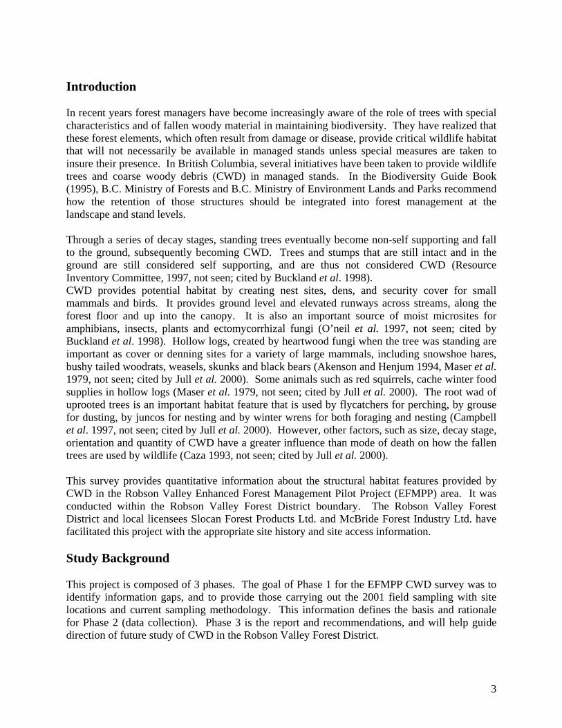
Analysis B: Mean Decay Class Mean Decay Class analysis for this study showed no significant difference between the TU and UN, with the exception of Class 1 in the ESSFmm1 and SBSvk, and Class 2 in the ESSFwk1 where there were more of these classes in TU compared to UN. The data for this analysis consists of counts of the number of classes that were found on a transect. These counts were modified to be counts per hundred-meter unit, rather than simply counts per transect. Following this, means of transects were taken to eliminate the pseudo replication within the plots Table 4 presents the p values for the t-tests. Asterisks mark those that are below 0.05. Figures 3-7 show the mean distribution of decay classes 1-5 by treatment unit for each subzone. For a description off Decay Classes, see Appendix 3. Figure 3: Mean Class 1 per 100m by treatment unit for each subzone
10
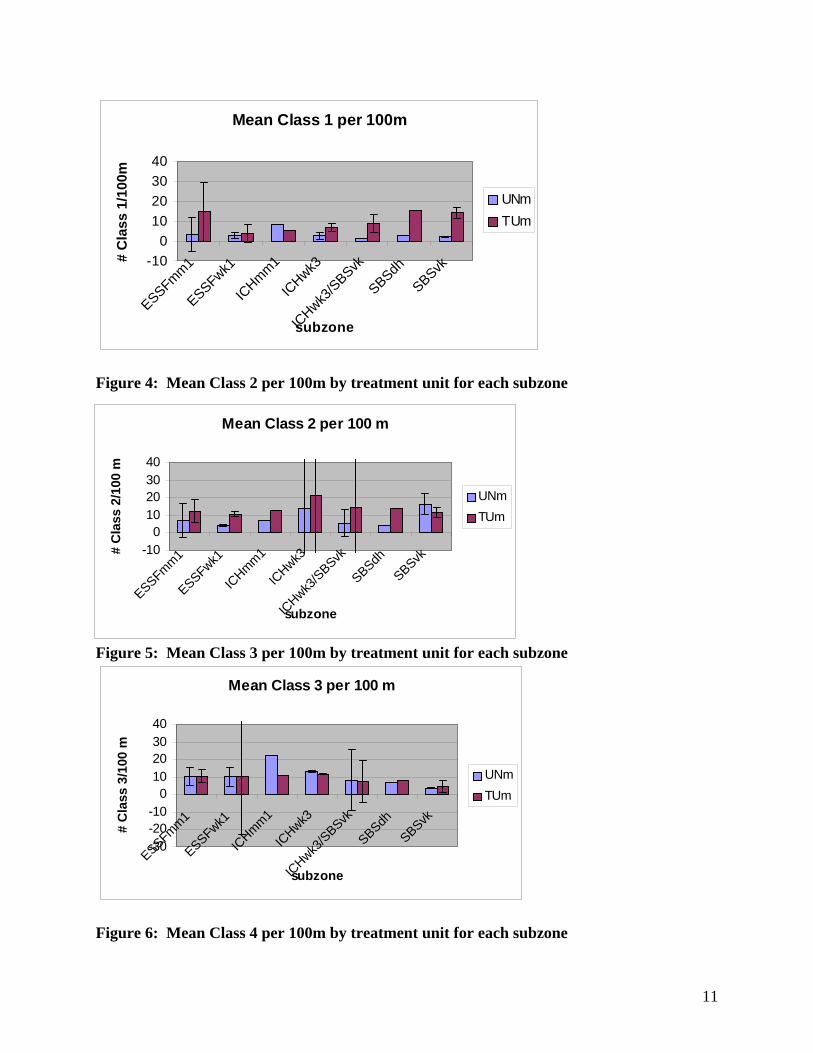
Figure 4: Mean Class 2 per 100m by treatment unit for each subzone
Figure 5: Mean Class 3 per 100m by treatment unit for each subzone
Mean Class 1 per 100m
-100
10203040
ESSFmm1
ESSFwk1
ICHmm1
ICHwk3
ICHwk3
/SBSvk
SBSdh
SBSvk
subzone
# C
lass
1/1
00m
UNmTUm
Mean Class 2 per 100 m
-100
10203040
ESSFmm1
ESSFwk1
ICHmm1
ICHwk3
ICHwk3
/SBSvk
SBSdhSBSvk
subzone
# C
lass
2/1
00 m
UNmTUm
Mean Class 3 per 100 m
-30-20-10
010203040
ESSFmm1
ESSFwk1
ICHmm1
ICHwk3
ICHwk3
/SBSvk
SBSdhSBSvk
subzone
# C
lass
3/1
00 m
UNmTUm
Figure 6: Mean Class 4 per 100m by treatment unit for each subzone
11
Mean Class 4 per 100 m
-20-10
010203040
ESSFmm1
ESSFwk1
ICHmm1
ICHwk3
ICHwk3
/SBSvk
SBSdhSBSvk
subzone
# C
lass
4/1
00m
UNmTUm
Figure 7: Mean Class 5 per 100m by treatment unit for each subzone
Mean Class 5 per 100 m
-10
-5
0
5
10
15
ESSFmm1
ESSFwk1
ICHmm1
ICHwk3
ICHwk3
/SBSvk
SBSdhSBSvk
subzone
# C
lass
/100
m
UNmTUm
Table 4: Results of testing the hypothesis of no difference between TU and UN for decay class. Class 1 Class 2 Class 3 Class 4 Class 5 ESSFmm1 p= 0.00397* p= 0.3175 p= 1 p= 1 p= 0.2474 ESSFwk1 p= 0.4226 p= 0.0339* p= 0.9374 p= 0.2664 p= 0.1835 SBSvk p= 0.02286* p= 0.3624 p= 0.7278 p= 0.7418 p= 0.8399
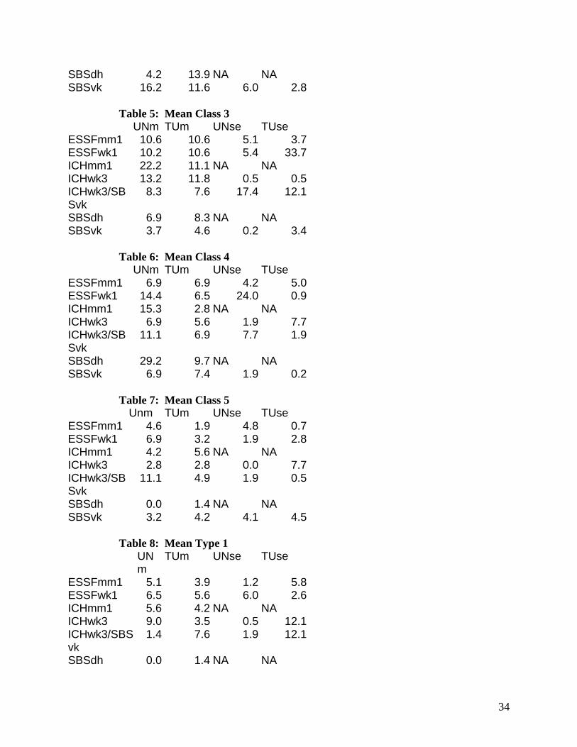
Analysis C: Mean Wildlife Types Analysis of Wildlife Types revealed Type 5 in the ESSFwk1 as the only subzone with a statistically significant difference between the TU and UN, with more Type 5 in UN. This analysis is similar to the last, except that it examines the mean number of types within the plots. Again, the counts were transformed to counts per 100 meters, and then averaged over transects. Figures 8-13 show the distribution of mean types per 100 m by treatment unit for each
12

subzone. Table 5 shows probability values for significance. For a description of Wildlife Types, see Appendix 4. Figure 8: Mean Type 1 per 100 m by treatment unit for each subzone
Mean Type1 per 100 m
-10
-5
0
5
10
15
ESSFmm1
ESSFwk1
ICHmm1
ICHwk3
ICHwk3
/SBSvk
SBSdhSBSvk
subzone
3 Ty
pe 1
/100
m
UNmTUm
Figure 9: Mean Type 2 per 100 m by treatment unit for each subzone
Mean Type 2 per 100 m
-40-30-20-10
0102030405060
ESSFmm1
ESSFwk1
ICHmm1
ICHwk3
ICHwk3
/SBSvk
SBSdhSBSvk
subzone
# Ty
pe 2
per
100
m
UNmTUm
13

Figure 10: Mean Type 3 per 100 m by treatment unit for each subzone
Mean Type 3 per 100 m
012345
ESSFmm1
ESSFwk1
ICHmm1
ICHwk3
ICHwk..
.SBSdh
SBSvk
subzone
# Ty
pe 3
/100
m
UNmTUm
Figure 11: Mean Type 4 per 100 m by treatment unit for each subzone
Mean Type4 per 100 m
-15-55
152535
ESSFmm1
ESSFwk1
ICHmm1
ICHwk3
ICHwk3
/SBSvk
SBSdh
SBSvk
subzone
# Ty
pe 4
/100
m
UNmTUm
Figure 12: Mean Type 5 per 100 m by treatment unit for each subzone
Mean Type5 per 100 m
-30
-20
-10
0
10
20
30
ESSFmm1
subzone
# Ty
pe 5
/100
m
UNmTUm
14
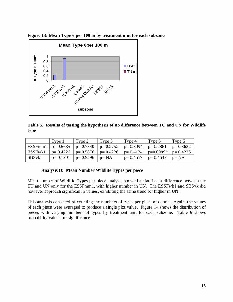
Figure 13: Mean Type 6 per 100 m by treatment unit for each subzone
Mean Type 6per 100 m
00.20.40.60.8
1
ESSFmm1
ESSFwk1
ICHmm1
ICHwk3
ICHwk3
/SBSvk
SBSdh
SBSvk
subzone
# Ty
pe 6
/100
m
UNmTUm
Table 5. Results of testing the hypothesis of no difference between TU and UN for Wildlife type Type 1 Type 2 Type 3 Type 4 Type 5 Type 6 ESSFmm1 p= 0.6685 p= 0.7840 p= 0.2752 p= 0.3094 p= 0.2861 p= 0.3632 ESSFwk1 p= 0.4226 p= 0.5876 p= 0.4226 p= 0.4134 p=0.0099* p= 0.4226 SBSvk p= 0.1201 p= 0.9296 p= NA p= 0.4557 p= 0.4647 p= NA
Analysis D: Mean Number Wildlife Types per piece
Mean number of Wildlife Types per piece analysis showed a significant difference between the TU and UN only for the ESSFmm1, with higher number in UN. The ESSFwk1 and SBSvk did however approach significant p values, exhibiting the same trend for higher in UN. This analysis consisted of counting the numbers of types per piece of debris. Again, the values of each piece were averaged to produce a single plot value. Figure 14 shows the distribution of pieces with varying numbers of types by treatment unit for each subzone. Table 6 shows probability values for significance.
15
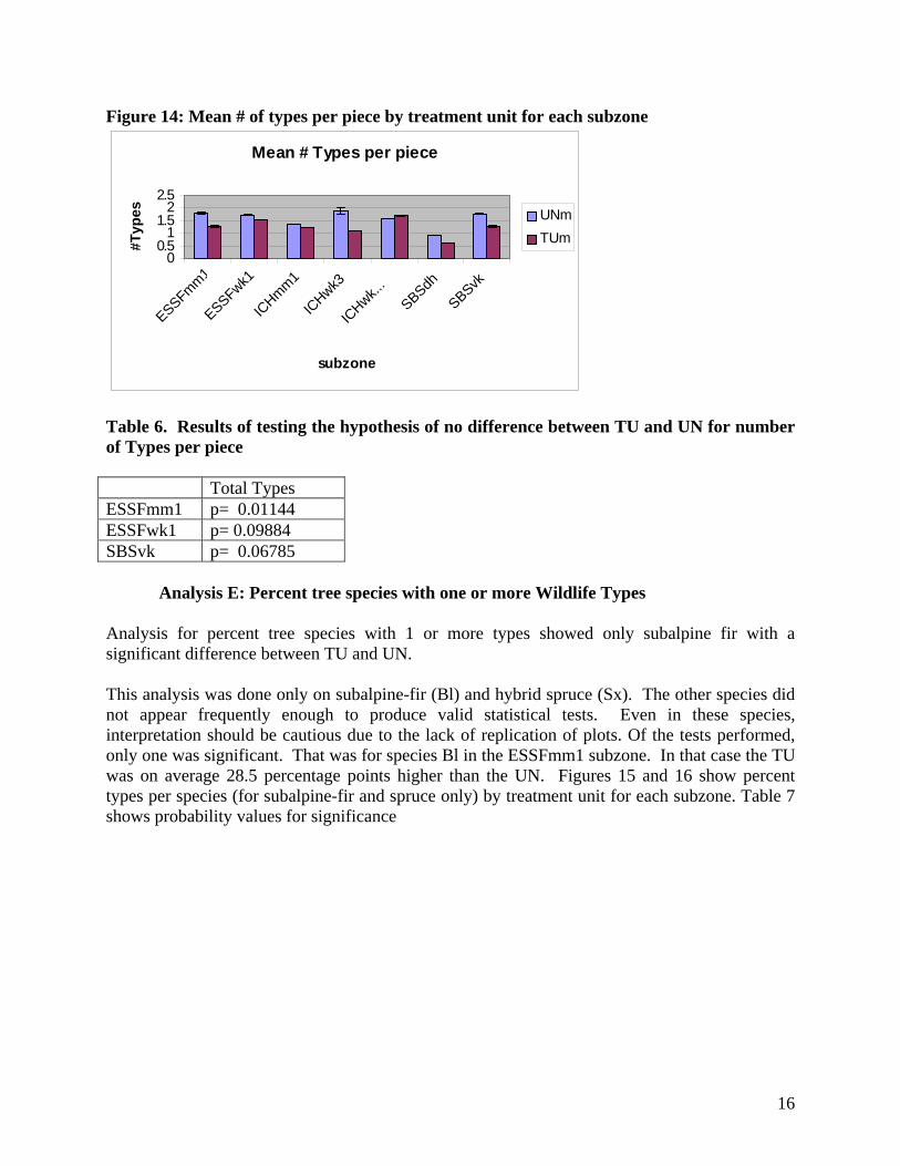
Figure 14: Mean # of types per piece by treatment unit for each subzone
Mean # Types per piece
00.5
11.5
22.5
ESSFmm1
ESSFwk1
ICHmm1
ICHwk3
ICHwk..
.SBSdh
SBSvk
subzone
#Typ
es UNmTUm
Table 6. Results of testing the hypothesis of no difference between TU and UN for number of Types per piece Total Types ESSFmm1 p= 0.01144 ESSFwk1 p= 0.09884 SBSvk p= 0.06785
Analysis E: Percent tree species with one or more Wildlife Types Analysis for percent tree species with 1 or more types showed only subalpine fir with a significant difference between TU and UN. This analysis was done only on subalpine-fir (Bl) and hybrid spruce (Sx). The other species did not appear frequently enough to produce valid statistical tests. Even in these species, interpretation should be cautious due to the lack of replication of plots. Of the tests performed, only one was significant. That was for species Bl in the ESSFmm1 subzone. In that case the TU was on average 28.5 percentage points higher than the UN. Figures 15 and 16 show percent types per species (for subalpine-fir and spruce only) by treatment unit for each subzone. Table 7 shows probability values for significance
16
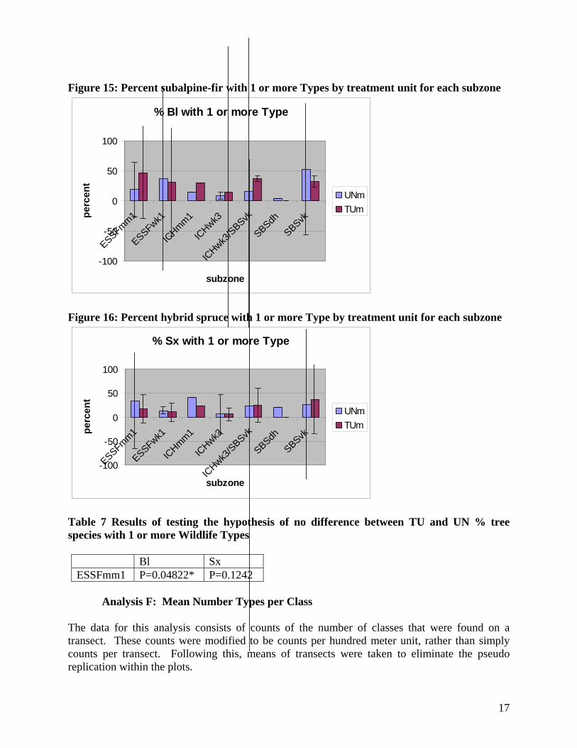
Figure 15: Percent subalpine-fir with 1 or more Types by treatment unit for each subzone
Figure 16: Percent hybrid spruce with 1 or more Type by treatment unit for each subzone
Table 7 Results of testing the hypothesis of no difference between TU and UN % tree species with 1 or more Wildlife Types
Bl Sx ESSFmm1 P=0.04822* P=0.1242
Analysis F: Mean Number Types per Class
The data for this analysis consists of counts of the number of classes that were found on a transect. These counts were modified to be counts per hundred meter unit, rather than simply counts per transect. Following this, means of transects were taken to eliminate the pseudo replication within the plots.
% Bl with 1 or more Type
-100
-50
0
50
100
ESSFmm1
ESSFwk1
ICHmm1
ICHwk3
ICHwk3
/SBSvk
SBSdh
SBSvk
subzone
perc
ent
UNmTUm
% Sx with 1 or more Type
-100
-50
0
50
100
ESSFmm1
ESSFwk1
ICHmm1
ICHwk3
ICHwk3
/SBSvk
SBSdh
SBSvk
subzone
perc
ent
UNmTUm
17
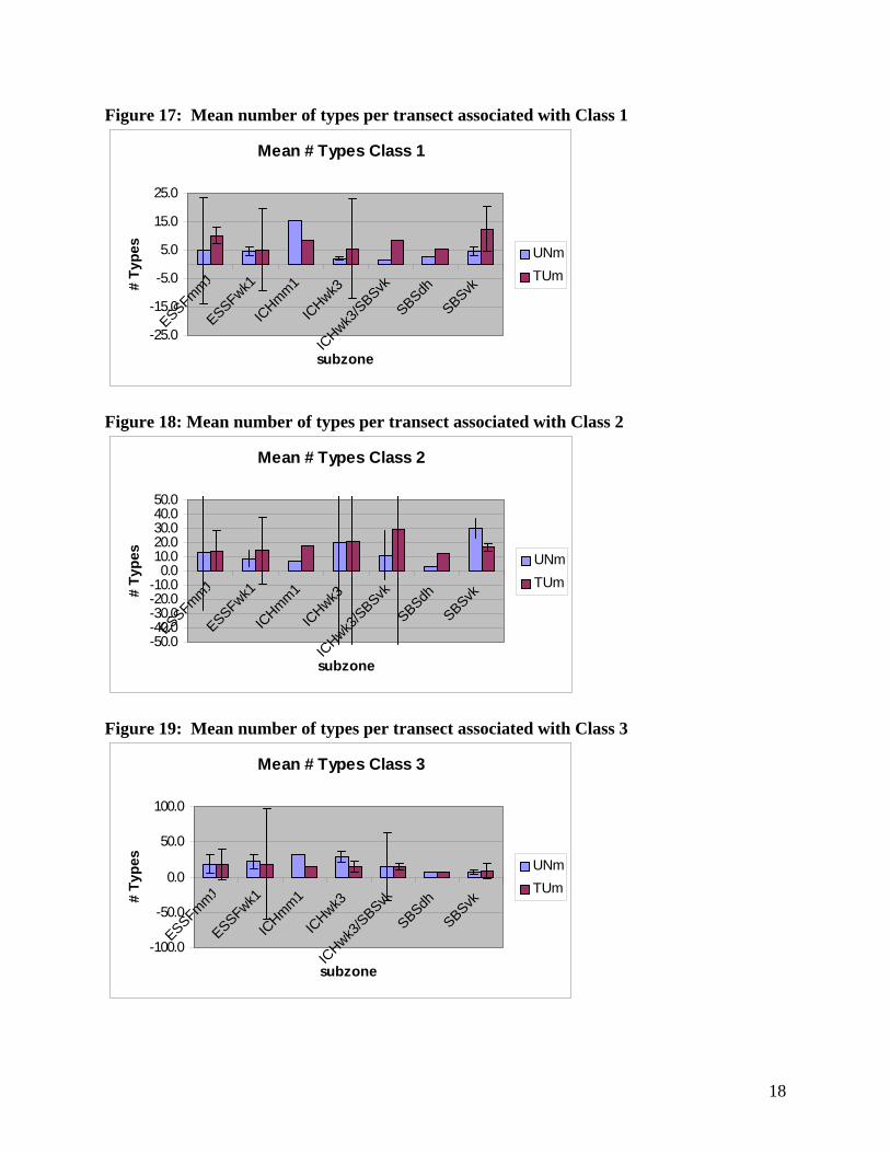
Figure 17: Mean number of types per transect associated with Class 1
Figure 18: Mean number of types per transect associated with Class 2
Figure 19: Mean number of types per transect associated with Class 3
Mean # Types Class 1
-25.0
-15.0
-5.0
5.0
15.0
25.0
ESSFmm1
ESSFwk1
ICHmm1
ICHwk3
ICHwk3
/SBSvk
SBSdh
SBSvk
subzone
# Ty
pes
UNmTUm
Mean # Types Class 2
-50.0-40.0-30.0-20.0-10.0
0.010.020.030.040.050.0
ESSFmm1
ESSFwk1
ICHmm1
ICHwk3
ICHwk3
/SBSvk
SBSdh
SBSvk
subzone
# Ty
pes
UNmTUm
Mean # Types Class 3
-100.0
-50.0
0.0
50.0
100.0
ESSFmm1
ESSFwk1
ICHmm1
ICHwk3
ICHwk3
/SBSvk
SBSdh
SBSvk
subzone
# Ty
pes
UNmTUm
18
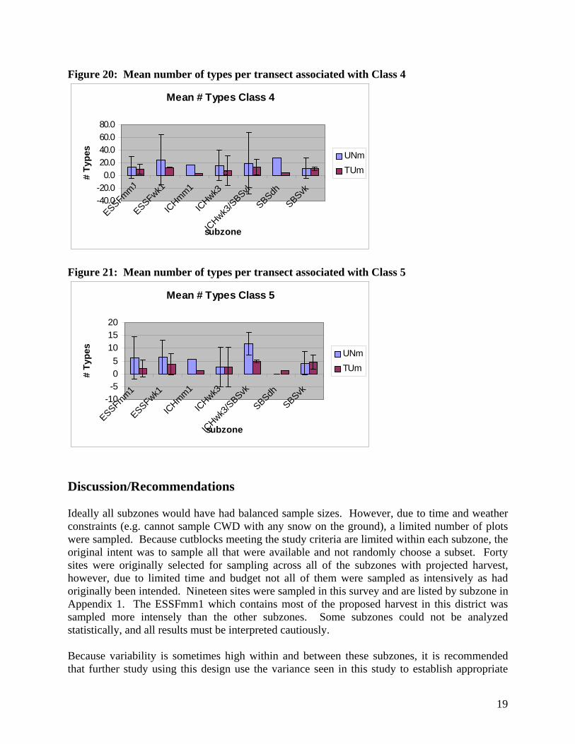
Figure 20: Mean number of types per transect associated with Class 4
Mean # Types Class 4
-40.0-20.0
0.020.040.060.080.0
ESSFmm1
ESSFwk1
ICHmm1
ICHwk3
ICHwk3
/SBSvk
SBSdh
SBSvk
subzone
# Ty
pes
UNmTUmc
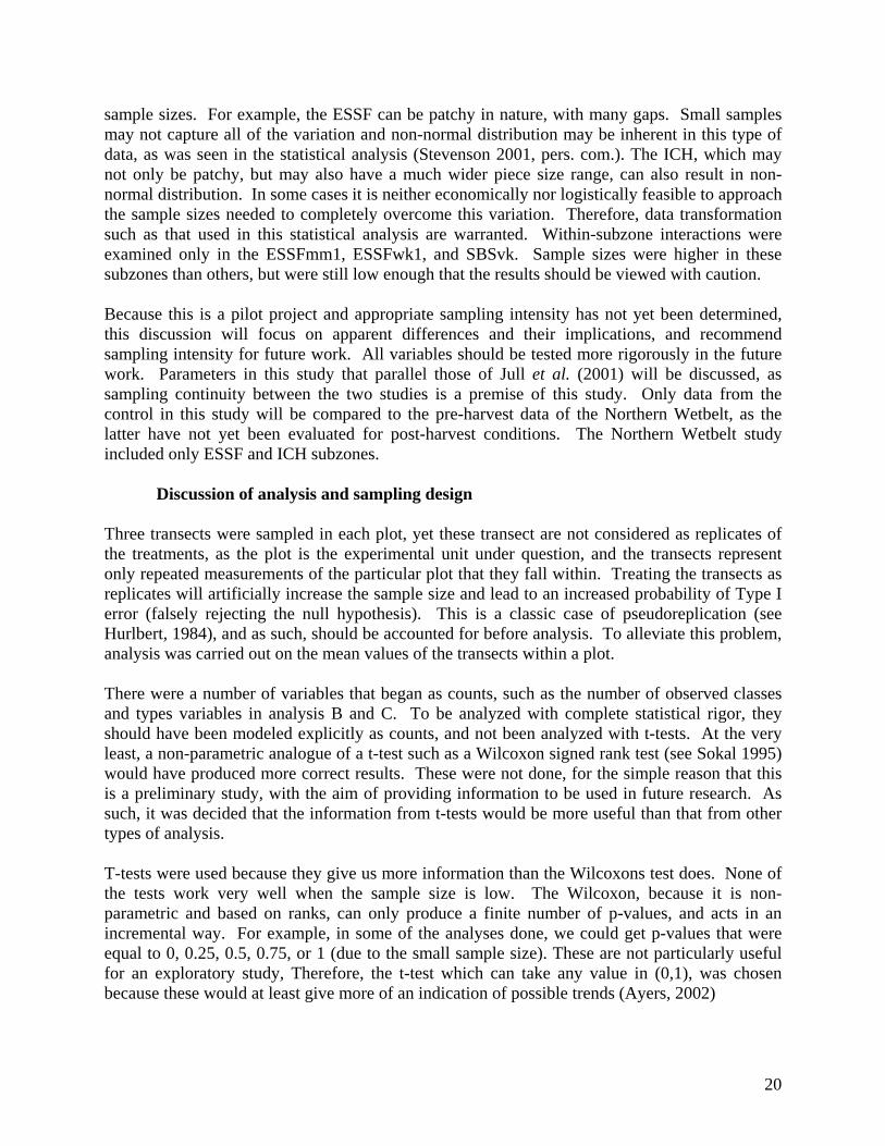
Figure 21: Mean number of types per transect associated with Class 5
Mean # Types Class 5
-10-505
101520
ESSFmm1
ESSFwk1
ICHmm1
ICHwk3
ICHwk3
/SBSvk
SBSdhSBSvk
subzone
# Ty
pes
UNmTUm
Discussion/Recommendations Ideally all subzones would have had balanced sample sizes. However, due to time and weather constraints (e.g. cannot sample CWD with any snow on the ground), a limited number of plots were sampled. Because cutblocks meeting the study criteria are limited within each subzone, the original intent was to sample all that were available and not randomly choose a subset. Forty sites were originally selected for sampling across all of the subzones with projected harvest, however, due to limited time and budget not all of them were sampled as intensively as had originally been intended. Nineteen sites were sampled in this survey and are listed by subzone in Appendix 1. The ESSFmm1 which contains most of the proposed harvest in this district was sampled more intensely than the other subzones. Some subzones could not be analyzed statistically, and all results must be interpreted cautiously. Because variability is sometimes high within and between these subzones, it is recommended that further study using this design use the variance seen in this study to establish appropriate
19
sample sizes. For example, the ESSF can be patchy in nature, with many gaps. Small samples may not capture all of the variation and non-normal distribution may be inherent in this type of data, as was seen in the statistical analysis (Stevenson 2001, pers. com.). The ICH, which may not only be patchy, but may also have a much wider piece size range, can also result in non-normal distribution. In some cases it is neither economically nor logistically feasible to approach the sample sizes needed to completely overcome this variation. Therefore, data transformation such as that used in this statistical analysis are warranted. Within-subzone interactions were examined only in the ESSFmm1, ESSFwk1, and SBSvk. Sample sizes were higher in these subzones than others, but were still low enough that the results should be viewed with caution. Because this is a pilot project and appropriate sampling intensity has not yet been determined, this discussion will focus on apparent differences and their implications, and recommend sampling intensity for future work. All variables should be tested more rigorously in the future work. Parameters in this study that parallel those of Jull et al. (2001) will be discussed, as sampling continuity between the two studies is a premise of this study. Only data from the control in this study will be compared to the pre-harvest data of the Northern Wetbelt, as the latter have not yet been evaluated for post-harvest conditions. The Northern Wetbelt study included only ESSF and ICH subzones.
Discussion of analysis and sampling design Three transects were sampled in each plot, yet these transect are not considered as replicates of the treatments, as the plot is the experimental unit under question, and the transects represent only repeated measurements of the particular plot that they fall within. Treating the transects as replicates will artificially increase the sample size and lead to an increased probability of Type I error (falsely rejecting the null hypothesis). This is a classic case of pseudoreplication (see Hurlbert, 1984), and as such, should be accounted for before analysis. To alleviate this problem, analysis was carried out on the mean values of the transects within a plot. There were a number of variables that began as counts, such as the number of observed classes and types variables in analysis B and C. To be analyzed with complete statistical rigor, they should have been modeled explicitly as counts, and not been analyzed with t-tests. At the very least, a non-parametric analogue of a t-test such as a Wilcoxon signed rank test (see Sokal 1995) would have produced more correct results. These were not done, for the simple reason that this is a preliminary study, with the aim of providing information to be used in future research. As such, it was decided that the information from t-tests would be more useful than that from other types of analysis. T-tests were used because they give us more information than the Wilcoxons test does. None of the tests work very well when the sample size is low. The Wilcoxon, because it is non-parametric and based on ranks, can only produce a finite number of p-values, and acts in an incremental way. For example, in some of the analyses done, we could get p-values that were equal to 0, 0.25, 0.5, 0.75, or 1 (due to the small sample size). These are not particularly useful for an exploratory study, Therefore, the t-test which can take any value in (0,1), was chosen because these would at least give more of an indication of possible trends (Ayers, 2002)
20
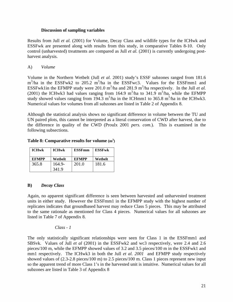
Discussion of sampling variables Results from Jull et al. (2001) for Volume, Decay Class and wildlife types for the ICHwk and ESSFwk are presented along with results from this study, in comparative Tables 8-10. Only control (unharvested) treatments are compared as Jull et al. (2001) is currently undergoing post-harvest analysis. A) Volume Volume in the Northern Wetbelt (Jull et al. 2001) study’s ESSF subzones ranged from 181.6 m3/ha in the ESSFwk2 to 205.2 m3/ha in the ESSFwc3. Values for the ESSFmm1 and ESSFwk1in the EFMPP study were 201.0 m3/ha and 281.9 m3/ha respectively. In the Jull et al. (2001) the ICHwk3 had values ranging from 164.9 m3/ha to 341.9 m3/ha, while the EFMPP study showed values ranging from 194.3 m3/ha in the ICHmm1 to 365.8 m3/ha in the ICHwk3. Numerical values for volumes from all subzones are listed in Table 2 of Appendix 8. Although the statistical analysis shows no significant difference in volume between the TU and UN paired plots, this cannot be interpreted as a literal conservation of CWD after harvest, due to the difference in quality of the CWD (Proulx 2001 pers. com.). This is examined in the following subsections. Table 8: Comparative results for volume (m3)
ICHwk ICHwk ESSFmm ESSFwk
EFMPP Wetbelt EFMPP Wetbelt 365.8 164.9-
341.9 201.0 181.6
B) Decay Class Again, no apparent significant difference is seen between harvested and unharvested treatment units in either study. However the ESSFmm1 in the EFMPP study with the highest number of replicates indicates that groundbased harvest may reduce Class 5 pieces. This may be attributed to the same rationale as mentioned for Class 4 pieces. Numerical values for all subzones are listed in Table 7 of Appendix 8.
Class - 1
The only statistically significant relationships were seen for Class 1 in the ESSFmm1 and SBSvk. Values of Jull et al (2001) in the ESSFwk2 and wc3 respectively, were 2.4 and 2.6 pieces/100 m, while the EFMPP showed values of 3.2 and 3.5 pieces/100 m in the ESSFwk1 and mm1 respectively. The ICHwk3 in both the Jull et al. 2001 and EFMPP study respectively showed values of (2.3-2.8 pieces/100 m) to 2.5 pieces/100 m. Class 1 pieces represent new input so the apparent trend of more Class 1’s in the harvested unit is intuitive. Numerical values for all subzones are listed in Table 3 of Appendix 8
21

Class - 2 Numbers seen in this study were comparable with those reported by Jull et al. (2001). The ESSFwk1 was the only subzone that showed a statistically significant difference, but there is an apparent trend toward more Class 2 pieces in the harvested area. The apparent increase in class 2’s in the TU is most likely a result of standing dead trees being pushed over, adding to the number of Class 2’s naturally on the forest floor. Numerical values for all subzones are listed in Table 4 of Appendix 8.
Class – 3 The EFMPP study showed similar results to that of the Jull et al. 2001 in the ESSF. Figures from the ICH subzones were some what comparable. There does not appear to be an apparent trend towards difference between Class 3 pieces in the harvested and unharvested units. This may be due to the fact that pieces that have reached this decay level in unharvested forest have done so as a function of already being on the forest floor, therefore harvesting activities do not significantly increase input. Numerical values for all subzones are listed in Table 5 of Appendix 8.
Class – 4 Class 4 in the ICHwk for both studies were comparable. The ESSFwk for the EFMPP was considerably higher than that of the Wetbelt study. The other subzone relationships for Class 4 are suspect due to low sample size. If further study reveals that there is indeed no significant difference between harvested and unharvested areas, it may be due to the lower position of these well established pieces on the forest floor, because they are often embedded in the ground. However it has been observed that groundbased harvesting can destroy a significant amount of Class 4 pieces due to their soft nature (author’s personal observation). For this reason it has been suggested based on other studies that if CWD were managed operationally in patches on cutblocks, that greater proportions of CWD with natural characteristics may be preserved (Lloyd 2001, pers. com.). Numerical values for all subzones are listed in Table 6 of Appendix 8.
Class - 5 Again, no apparent significant difference is seen between harvested and unharvested treatment units in either study. However the ESSFmm1 in the EFMPP study with the highest number of replicates indicates that groundbased harvest may reduce Class 5 pieces. This may be attributed to the same rationale as mentioned for Class 4 pieces. Numerical values for all subzones are listed in Table 7 of Appendix 8. Table 9: Comparative results for decay class (frequency/100 m)
Class ICHwk ICHwk ESSFwk ESSFwk
EFMPP Wetbelt EFMPP Wetbelt Class 1 2.80 2.30-
2.80 3.20 2.40
22
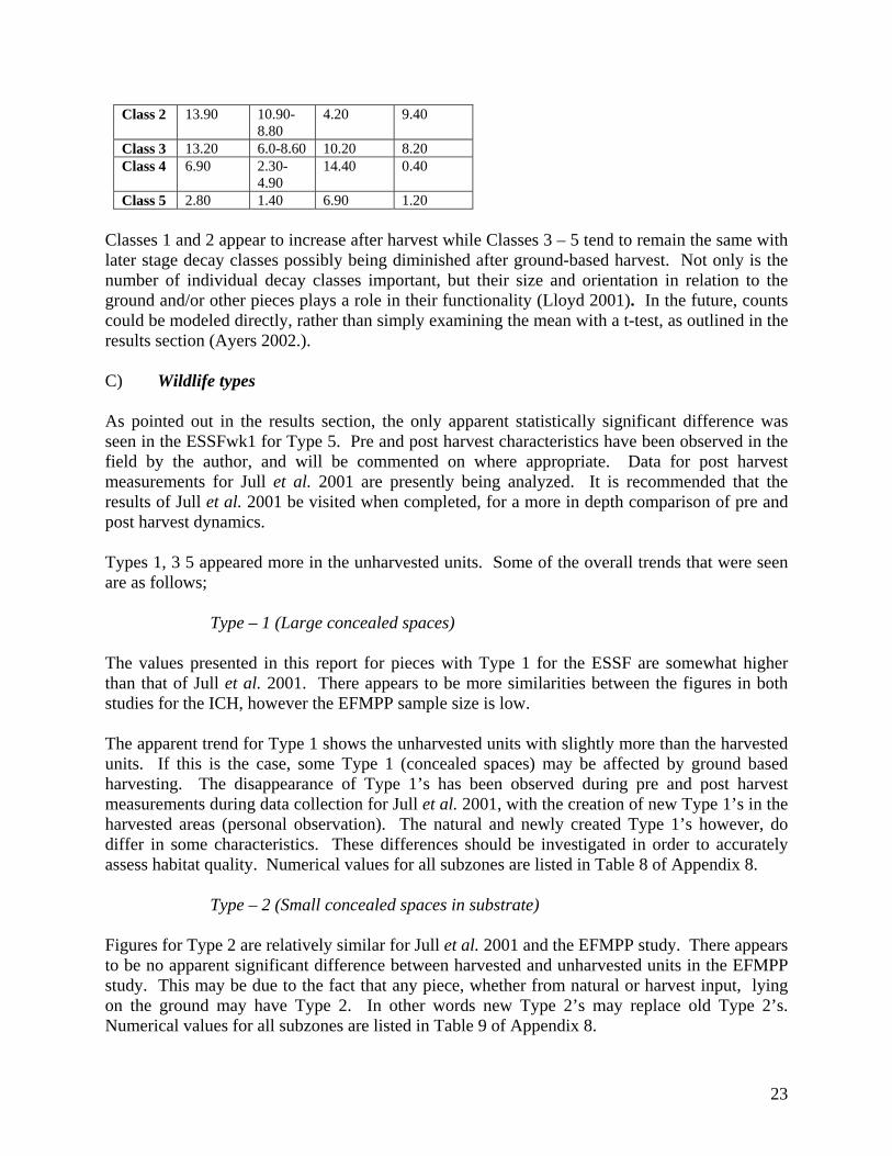
Class 2 13.90 10.90-8.80
4.20 9.40
Class 3 13.20 6.0-8.60 10.20 8.20 Class 4 6.90 2.30-
4.90 14.40 0.40
Class 5 2.80 1.40 6.90 1.20 Classes 1 and 2 appear to increase after harvest while Classes 3 – 5 tend to remain the same with later stage decay classes possibly being diminished after ground-based harvest. Not only is the number of individual decay classes important, but their size and orientation in relation to the ground and/or other pieces plays a role in their functionality (Lloyd 2001). In the future, counts could be modeled directly, rather than simply examining the mean with a t-test, as outlined in the results section (Ayers 2002.). C) Wildlife types As pointed out in the results section, the only apparent statistically significant difference was seen in the ESSFwk1 for Type 5. Pre and post harvest characteristics have been observed in the field by the author, and will be commented on where appropriate. Data for post harvest measurements for Jull et al. 2001 are presently being analyzed. It is recommended that the results of Jull et al. 2001 be visited when completed, for a more in depth comparison of pre and post harvest dynamics. Types 1, 3 5 appeared more in the unharvested units. Some of the overall trends that were seen are as follows; Type – 1 (Large concealed spaces) The values presented in this report for pieces with Type 1 for the ESSF are somewhat higher than that of Jull et al. 2001. There appears to be more similarities between the figures in both studies for the ICH, however the EFMPP sample size is low. The apparent trend for Type 1 shows the unharvested units with slightly more than the harvested units. If this is the case, some Type 1 (concealed spaces) may be affected by ground based harvesting. The disappearance of Type 1’s has been observed during pre and post harvest measurements during data collection for Jull et al. 2001, with the creation of new Type 1’s in the harvested areas (personal observation). The natural and newly created Type 1’s however, do differ in some characteristics. These differences should be investigated in order to accurately assess habitat quality. Numerical values for all subzones are listed in Table 8 of Appendix 8.
Type – 2 (Small concealed spaces in substrate) Figures for Type 2 are relatively similar for Jull et al. 2001 and the EFMPP study. There appears to be no apparent significant difference between harvested and unharvested units in the EFMPP study. This may be due to the fact that any piece, whether from natural or harvest input, lying on the ground may have Type 2. In other words new Type 2’s may replace old Type 2’s. Numerical values for all subzones are listed in Table 9 of Appendix 8.
23
Type – 3 (Small concealed spaces above ground level) Type 3 in the ESSF and ICH for Jull et al. 2001 was highly variable. There is an apparent trend for higher numbers of Type 3 in the unharvested unit for the ESSF and ICH, and extremely low numbers in the SBS in the EFMPP study. The former may be due to the presence of upturned root-wads (often associated with Type 3) found intact in the unharvested units, that may be destroyed in the harvested units. Numerical values for all subzones are listed in Table 10 of Appendix 8.
Type 4 (Long concealed spaces in substrate) Values for the ICH and ESSF for both studies appear to be similar. There appears to be no apparent significant difference between the harvested and unharvested units in the EFMPP study. As seen with Type 2, there may simply be a replacement of natural Type 4’s with Type 4’s associated with new input from harvesting. Numerical values for all subzones are listed in Table 11 of Appendix 8.
Type – 5 (Large or elevated structures/runways) ESSF and ICH values were similar for both studies. The EFMPP study showed no apparent significant difference between the harvested and unharvested units except for the ESSFwk1 where 12.0 Type 5’s per 100 m and 7.4 per 100 m were observed in the unharvested unit. If more rigorous testing revealed that the control indeed had more than the clearcut, it may be due to the piece length minimum data collection protocol of 4-5 m depending on evident runway value, that was used in both studies. In Jull et al. 2001, the ESSFwc3 showed almost twice as many Type 5’s in the control as in the treatment units, although neither treatment unit was a clearcut. Numerical values for all subzones are listed in Table 12 of Appendix 8
Type – 6 (Invertebrates in wood or under bark)
Although numbers appeared somewhat similar between both studies, they were done at different times of the year. Jull et al. 2001 was done in early to mid summer, while this study was done in late fall. The lower temperature for the EFMPP study would no doubt have an effect on the number of invertebrates observed. For example, in the clear cut where surface temperature is warmer, carpenter ants are usually seen at higher numbers. Aspect may have an influence on the amount of invertebrates seen at this time of year, again suggesting that there is a need to have more replicates in order to capture this variation. Numerical values for all subzones are listed in Table 13 of Appendix 8 Table 10: Comparative results for wildlife Types (frequency/100 m)
Types ICHwk ICHwk ESSFwk ESSFwk
EFMPP Wetbelt EFMPP Wetbelt Type 1 9.0 2.50-6.0 6.50 2.0
24
Type 2 31.3 19.20-25.00
31.9 20.7
Type 3 4.20 0.50-2.10
0.00 0.40
Type 4 20.10 14.10-17.60
15.30 18.20
Type 5 5.60 6.90-10.90
12.00 5.40
Type 6 0.00 0.20 0.23 0.10 D) Mean number of Types per piece The number of wildlife Types found per piece is a variable that allows a value to be attached to each piece. The ESSFmm1 showed a significant difference in the number of Types found per piece, with mean values of 1.8 in the unharvested units and 1.3 in the harvested units. The ESSFwk1, and SBSvk had very similar results and approached significant p values. Certain structures such as large concealed spaces (Type 1), raised cavities (Type 3), and runways (Type 5), appear to show up less frequently in the harvested units with this data set. These structures are easily destroyed through harvesting activities such as movement along skid trails and landings (personal observation). The disappearance of some of these structures may explain the lower number of types per piece found in the harvested units. E) Percent Types per tree species This analysis included only subalpine-fir (Bl) and hybrid spruce (Sx) in the ESSFmm1. There was a significant difference between harvested and unharvested units for Bl. Perhaps because Bl is more likely to be non-merchantable than Sx, and therefore more likely to be left in the cutblock. Bl decays faster than Sx, so nearly half the Types in the harvested unit may not persist long in relation to rotation length. In the unharvested unit Bl had 19% of the Types, while in the harvested unit it had 47.5% of the Types. This observation by itself does not tell us much, however, knowing which tree species has most of the Types, may allow for future predictions of the longevity of structures based on species decay rates (Parminter 2001). It is recommended that future work be based on sample sizes that are large enough to accurately examine this distribution. F) Mean Number of Types per Class In the harvested units, early Decay Classes appear by observation to have more types associated with them than later Decay Classes. Between Class differences should be tested in future work to determine how the natural dynamic compares to the harvested dynamic over the decay class continuum.. Later Decay Classes such as Class 4 and 5 may be more prone to loosing types through destruction or having them covered up by slash (this needs to be statistically analyzed). Although the study overall was statistically limited due to low sample size and the lack of replication in some subzones, the ESSFmm1 was the strongest. This subzone is targeted for the highest timber removal in the Robson Valley Forest District. The addition of replicates to each subzone in this study is recommended before making concrete conclusions about the state of
25
26
CWD in harvested and unharvested areas. Balanced sample sizes between subzones are also recommended so that between subzone effects may be examined.
General summary of results • No significant difference was detected for volume between the clearcut and unharvested
units. • The presence of Decay Classes 1 and 2 appears to be higher in the harvested units. • Harvesting may reduce the presence of Decay Class 4 and 5 pieces, and wildlife habitat
Types 1, 3, and 5. • More CWD Wildlife Types are associated with pieces in the unharvested areas. • Observation suggests that as decay class increases there are fewer types associated with each
piece in the harvested units than in the unharvested.
Recommendations The influence that the CWD structure left in clearcuts after harvest has on wildlife habitat, will no doubt change over time. If we are to manage for specific wildlife species we not only need to know their habitat requirements, but also what is and will be available for them under a variety disturbances. Some wildlife may not immediately utilize CWD left in clearcuts, while others such as winter wrens, dark eyed junkos and Clark’s nutcrackers may take advantage of the newly created structures (personal observation). No matter how much CWD is left in cutblocks, voles will not inhabit these areas until total vegitative ground cover has been re-established. In the absence of proper ground structural complexity, adequate internal connectivity, and prey base (i.e. voles), mustelids such as martin (Martes americana) will not venture in openings, even if piles of debris are spread across cutblocks (Proulx 2001-1). Based on this, CWD wildlife use should be monitored over time to capture the frequency of use through stand initiation/regeneration and further succession. This study serves as a window to view areas of CWD structure and dynamics in relation to the subzones of the Robson Valley Forest District that need to be further understood. Surveys must be conducted on a larger scale in order to overcome ecological variation that is highly inherent to this natural disturbance type (NDT 1), and be able to more accurately predict the implications of CWD management. The following recommended sampling intensities should be used in subsequent CWD studies within these subzones. Future work should also include the following: • The following rationale guided the calculation of suggested sampling intensity:
-sample size calculations are based on Volume data for the ESSF -an estimate for variance of 0.818 was used. This is the variance of the difference between TU and UN in the ESSF groups based on the cube root variable
27
-For a difference between the means 0.50 was used. This is slightly larger than some of the differences seen in the data.
The following formula was used to calculate sample size n=tP
2P*s/ dP
2P
where t is the appropriate critical value of the t distribution. The estimate of the variance is given by sP
2P, and d represents the difference between the means of the two groups.
for 90% confidence, n= (2.13P
2P)*.818/(0.5)P
2P = 15 plots
and for 95% n= 1.8 P
2P*.818/0.5 P
2P = 11 plots
These numbers represent the number of plots to sample, and not the number of transects within a plot. For inventory purposes a sample size based on a 95% confidence interval may be logistically impractical. Therefore, sample size based on a 90% confidence interval is also presented.
• CWD sampling in cutblocks with harvest methods and silviculture systems (e.g. group
selection, single tree selection etc…) not covered in the 2001 survey. • Waste and residue surveys should be conducted to determine how varying levels of
utilization effect CWD characteristics on cutblocks. • CWD should be looked at across a variety of site prep methods, as these methods have a
direct impact on the levels and condition of CWD on a cut-block. • Wildlife use should be measured not only to detect when use in the cutblock begins, but also
which animal species use the structures the most. • Investigate the difference in structural characteristics between the same Wildlife Types found
under natural conditions and those created by logging, to determine if the sampling protocol should account for any difference in quality.
• Tracking temporal changes in longevity or functionality of Wildlife Types in relation to
decay rate will supply information that can be used to predict changes in the habitat quality of a forest floor over time.
• Specific CWD Types associated with particular decay classes should be analyzed to
determine if Types are natural or associated with new input, as there may be a difference in quality between the two.

28
• Between subzone comparisons should be conducted to determine which particular harvesting
practices are most appropriate for each ecosystem. • The knowledge of what structures are there and how they are effected by harvest should be
complemented with the knowledge of who uses what and when. For information related to wildlife habitat use of different forest structures see Gillingham (2002). Use of the structures should be examined across a variety of successional and seral stages after harvest.
• The effects of a variety of harvesting machinery on CWD should be examined as seen in
Lloyd (2002).

Literature Cited
Atkenson, J.J. and M.G. Henjum. 1994. Black bear den sites in the Starkey Study area. Natural Resource News 4(2): 1-2. Blue Mountains Natural Resource Institute.
Ayers, Dieter. 2002. Statistical Consultant. University of Northern British Columbia. B.C. Ministry of Forests. 1996. A Draft Field Guide Insert for Site Identification and
Interpretation for the Rocky Mountain Trench. Buckland, N. M. Martin, L. Beaudry, J. Stork, and edited by D. Lousier, 1998. Inventories of
Wildlife Trees and Coarse Woody Debris Resources and Associated Birds and Small Mammals in the Major Timber Types of the Vanderhoof Forest District. Madrone Consultants Ltd., #220-1990 S. Oglivie Street, Prince George, BC, V2N 1X1.
Campbell, R.W., N.K. Dawe, I. McTaggart-Cowen, J.M. Cooper, G.W. Kaiser. The Birds of
British Columbia. Vol. III. Passerines: Flycatchers through vireos. UBC Press, Vancouver, BC.
Caza, C.L. 1993. Woody debris in the forests of British Columbia: a review of the literature
and current research. B.C. Min. For. Land Manage. Rep. 78. Victoria. Gillingham,M.P., and K.L. Parker. 2001. Summary report for the first year of the Project on
Lifeform Classification. Contribution agreement report to Lignum, Ltd. 10 Dec. 21 pp. + 337 pp. appendices.
Harrison, M. and DeLong C. 2000. A Comparison of Ecological Characteristics for Age Class 8
and 9 Stands in the ICHwk3 and ESSFwk2: Development of an Index to Assess Old Growth Features. Prepared for the Robson Valley Enhanced Forest Management Pilot Project.
Hogget, V. 2000. Western Hemlock Looper and Forest Disturbance in the ICHwk3 of the
Robson Valley. Faculty of Forestry, University of British Columbia. Hoyles, S. 2001, personal communication. MoF Region NIVMA representative, Silviculture
Vegetation Officer, Prince George Forest Region. Hurlbert, Stuart H. 1984, “Psuedoreplication and the design of ecological field experiments”
Ecological Monographs, 54(2), 1984, pp187-211. Jull, M. and S.K. Stevenson, 1999. A descriptive Summary of pre-harvest data collection for the
Northern Rockies Wet-belt ICH/ESSF Silviculture Systems Project Phase III. University of Northern British Columbia.
29

Jull, M. S.K. Stevenson, A. Eastham, and P.Sanborn, 2000. Effects of Partial-cut Silviculture Systems in Northern ICH and ESSF Stands on Stand dynamics and Structural Biodiversity. Working plan for the Northern Rockies Wet-belt ICH/ESSF Silviculture Systems Project Phase III. University of Northern British Columbia.
Jull, M. S.K. Stevenson, Bruce Rogers, Paul Sandborn, and Andrea Eastham, 2001. Northern
Wetbelt Silviculture Systems Project. Summary of Initial pre-harvest Conditions and Harvest Treatments (Establishment Report-First approximation). University of Northern British Columbia.
Keisker, D.G. 2001. Types of Wildlife Trees and Coarse Woody Debris Required by Wildlife
of North Central British Columbia. MoF. Working Paper No. 50. Victoria Lloyd, R. 2001. Northern Silviculture Committee workshop 2001. Optimizing wildlife trees and
coarse woody debris retention at the stand and landscape level. Taken from comments noted at post presentation question period. University of Northern BC.
Marshall, P.L. 1999. Using line intersect sampling to determine the volume of odd-shaped
pieces of coarse woody debris: an explanation of the Vegetation Resource Inventory formula. Department of Forest Resources Management, University of British Columbia. Unpublished report.
Marshall, P.L., G. Davis, and V.M Lemay 2000. Using Line Intersect Sampling for CWD.
Forest Research Technical Report. B.C. Min. For., Vancouver Forest Region, 2100 Labieux Rd Nanaimo, BC, V9T 6E9
Maser, C., R.G. Anderson, K. Cromack, Jr., J.T. Williams and R.E. Martin. 1979. Dead and
down woody material. Pp. 78-95 in Thomas, J.W. (tech. Ed.) Wildlife habitats in managed forests: the Blue Mountains of Oregon and Washington, DC.
Oneil,. E., Beaudry L., Whittaker C., Kessler W., and Lousier J. D. 1997. Ecology and
Management of Douglas-fir at at the Northern Limits of its Range. A Problem Analysis and Interim Management Strategy. University of Northern British Columbia. Prince George, BC.
Parminter, John 2001. Coarse Woody Debris Decomposition-principles, rates and models,
Presented at the Northern Silviculture Committee workshop 2001, Optimizing wildlife trees and coarse woody debris retention at the stand and landscape level. University of Northern BC.
Proux, Gilbert 2001. Northern Silviculture Committee workshop 2001. Optimizing wildlife
trees and coarse woody debris retention at the stand and landscape level. Taken from comments noted at post presentation question period. University of Northern BC.
30

Proux, Gilbert-1 2001. Coarse Woody Debris and small mammal populations in the sub-boreal spruce biogeoclimatic zone of Ft. St. James Forest District, British Columbia Presented at the Northern Silviculture Committee workshop 2001. Optimizing wildlife trees and coarse woody debris retention at the stand and landscape level.. University of Northern BC.
Resource Inventory Committee. 1997. Standard Inventory Methodologies for Components of
British Columbia’s Biodiversity: Ground Sampling Procedures. Ministry of Environment, Lands and Parks; Wildlife Branch. Victoria, British Columbia.
Rogers, Bruce 2001. Field Data Collection Protocol Manual for Robson Valley EFMPP CWD
Survey 2001. Adapted from Jull, M., Stevenson, S., and Rogers B. Field Data Collection Protocol Manual for the Northern Wetbelt Silviculture Systems Project 2001.
Sokal, Robert R., and F. James Rohlf, “Biometry, 3rd edition”,1995,
W.H.Freeman and Company, New York Stevenson, S.K. 2001. Personal Communication. Silvafauna Research. Prince George BC Stevenson, S.K. 1999. Biodiversity Assessments at Silviculture Systems Sites, Summer 1998.
Silvifauna Research, 101 Burden Street, Prince George, BC, V2M 2G8 Stevenson, S.K. 2001. personal communication. Silvifauna Research, 101 Burden Street,
Prince George, BC, V2M 2G8 Sokal, R.R. and F.J Rohlf 1995. Biometry. The Principle of Statistics in Biological Research,
3rd Addition. State University of New York and Stony Brook. Van Wagner, C.E. 1982. Practical aspects of the line intersect method. Can. For. Serv. Info.
Rep. PI-X-12. Petawawa National Forestry Institute, Chalk River, Ontario.
31
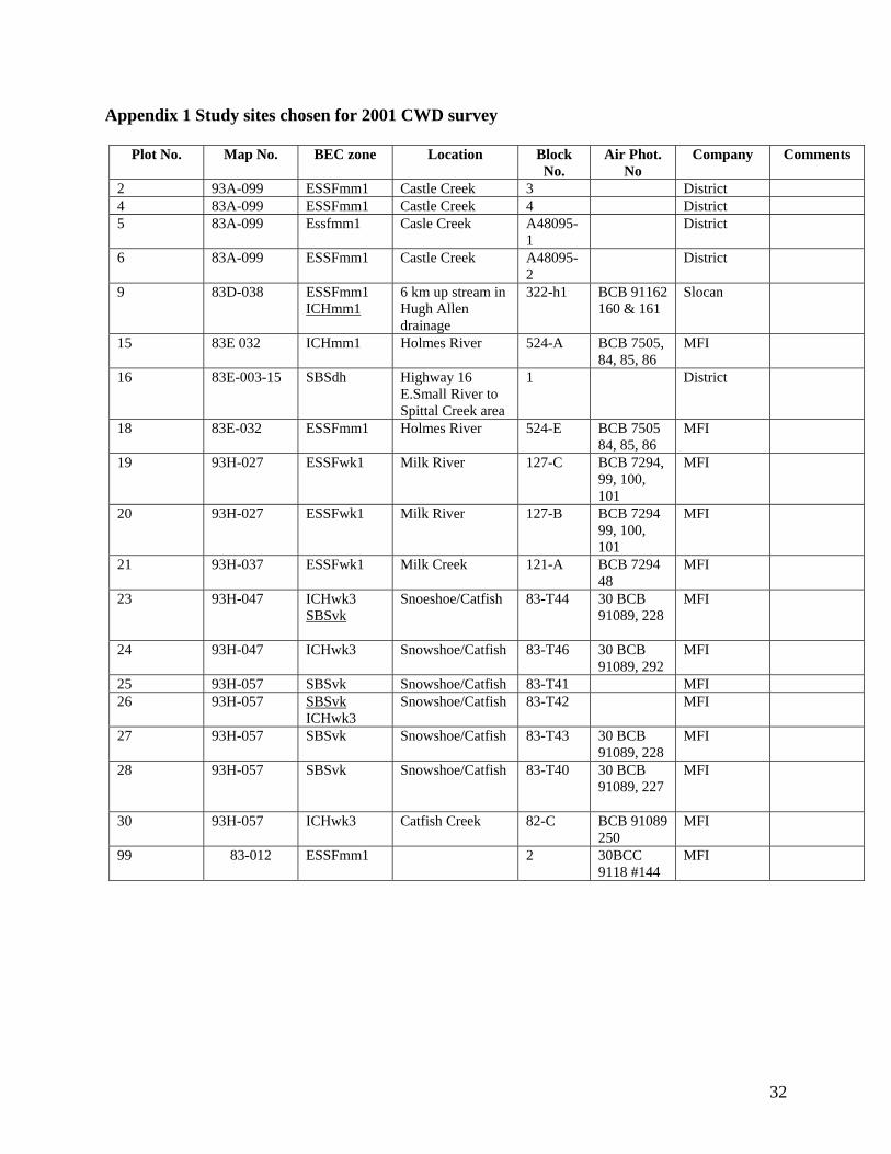
Appendix 1 Study sites chosen for 2001 CWD survey
Plot No. Map No. BEC zone Location Block No.
Air Phot. No
Company Comments
2 93A-099 ESSFmm1 Castle Creek 3 District 4 83A-099 ESSFmm1 Castle Creek 4 District 5 83A-099 Essfmm1 Casle Creek A48095-
1 District
6 83A-099 ESSFmm1 Castle Creek A48095-2
District
9 83D-038 ESSFmm1 ICHmm1
6 km up stream in Hugh Allen drainage
322-h1 BCB 91162 160 & 161
Slocan
15 83E 032 ICHmm1 Holmes River 524-A BCB 7505, 84, 85, 86
MFI
16 83E-003-15 SBSdh Highway 16 E.Small River to Spittal Creek area
1 District
18 83E-032 ESSFmm1 Holmes River 524-E BCB 7505 84, 85, 86
MFI
19 93H-027 ESSFwk1 Milk River 127-C BCB 7294, 99, 100, 101
MFI
20 93H-027 ESSFwk1 Milk River 127-B BCB 7294 99, 100, 101
MFI
21 93H-037 ESSFwk1 Milk Creek 121-A BCB 7294 48
MFI
23 93H-047 ICHwk3 SBSvk
Snoeshoe/Catfish 83-T44 30 BCB 91089, 228
MFI
24 93H-047 ICHwk3 Snowshoe/Catfish 83-T46 30 BCB 91089, 292
MFI
25 93H-057 SBSvk Snowshoe/Catfish 83-T41 MFI 26 93H-057 SBSvk
ICHwk3 Snowshoe/Catfish 83-T42 MFI
27 93H-057 SBSvk Snowshoe/Catfish 83-T43 30 BCB 91089, 228
MFI
28 93H-057 SBSvk Snowshoe/Catfish 83-T40 30 BCB 91089, 227
MFI
30 93H-057 ICHwk3 Catfish Creek 82-C BCB 91089 250
MFI
99 83-012 ESSFmm1 2 30BCC 9118 #144
MFI
32
Appendix 2: Mean Values of variables
Table 1: Cube Root Volumes UNm Tum ESSFmm1 5.9 6.6 0.3 0.2ESSFwk1 6.6 6.2 0.1 0.1ICHmm1 5.8 5.5 NA NA ICHwk3 7.2 6.9 0.3 0.0ICHwk3/SBSvk
6.2 6.5 0.0 0.7
SBSdh 6.8 5.2 NA NA SBSvk 5.8 6.2 0.2 0.1
Table 2: Volume (m3) UNm TUm
ESSFmm1 201.0 286.5 ESSFwk1 281.9 236.6 ICHmm1 194.3 167.3 ICHwk3 365.8 323.6 ICHwk3/SBSvk
243.6 277.9
SBSdh 320.5 144.4 SBSvk 198.3 237.6
Table 3: Mean Class 1
UNm TUm UNse TUse ESSFmm1 3.5 14.8 8.7 14.7ESSFwk1 3.2 4.2 1.5 4.5ICHmm1 8.3 5.6 NA NA ICHwk3 2.8 6.9 1.9 1.9ICHwk3/SBSvk
1.4 9.0 0.0 4.3
SBSdh 2.8 15.3 NA NA SBSvk 2.3 14.4 0.2 2.8
Table 4: Mean Class 2 UNm TUm UNse TUse
ESSFmm1 7.2 12.3 9.6 6.6ESSFwk1 4.2 10.6 0.6 1.5ICHmm1 6.9 12.5 NA NA ICHwk3 13.9 21.5 123.5 174.1ICHwk3/SBSvk
5.6 14.6 7.7 81.5
33
SBSdh 4.2 13.9 NA NA SBSvk 16.2 11.6 6.0 2.8
Table 5: Mean Class 3 UNm TUm UNse TUse
ESSFmm1 10.6 10.6 5.1 3.7ESSFwk1 10.2 10.6 5.4 33.7ICHmm1 22.2 11.1 NA NA ICHwk3 13.2 11.8 0.5 0.5ICHwk3/SBSvk
8.3 7.6 17.4 12.1
SBSdh 6.9 8.3 NA NA SBSvk 3.7 4.6 0.2 3.4
Table 6: Mean Class 4 UNm TUm UNse TUse
ESSFmm1 6.9 6.9 4.2 5.0ESSFwk1 14.4 6.5 24.0 0.9ICHmm1 15.3 2.8 NA NA ICHwk3 6.9 5.6 1.9 7.7ICHwk3/SBSvk
11.1 6.9 7.7 1.9
SBSdh 29.2 9.7 NA NA SBSvk 6.9 7.4 1.9 0.2
Table 7: Mean Class 5 Unm TUm UNse TUse
ESSFmm1 4.6 1.9 4.8 0.7ESSFwk1 6.9 3.2 1.9 2.8ICHmm1 4.2 5.6 NA NA ICHwk3 2.8 2.8 0.0 7.7ICHwk3/SBSvk
11.1 4.9 1.9 0.5
SBSdh 0.0 1.4 NA NA SBSvk 3.2 4.2 4.1 4.5
Table 8: Mean Type 1 UNm
TUm UNse TUse
ESSFmm1 5.1 3.9 1.2 5.8ESSFwk1 6.5 5.6 6.0 2.6ICHmm1 5.6 4.2 NA NA ICHwk3 9.0 3.5 0.5 12.1ICHwk3/SBSvk
1.4 7.6 1.9 12.1
SBSdh 0.0 1.4 NA NA
34

SBSvk 9.3 3.7 16.9 6.0
Table 9: Mean Type 2 UNm TUm UNse TUse
ESSFmm1 27.3 28.2 26.6 12.0ESSFwk1 31.9 29.6 8.4 16.9ICHmm1 47.2 26.4 NA NA ICHwk3 31.3 34.0 23.6 23.6ICHwk3/SBSvk
34.7 36.1 17.4 69.4
SBSdh 25.0 15.3 NA NA SBSvk 27.8 33.8 12.2 22.1
Table 10: Mean Type 3 UNm TUm UNse TUse
ESSFmm1 1.4 0.0 1.3 0.0ESSFwk1 0.0 0.9 0.0 0.9ICHmm1 1.4 0.0 NA NA ICHwk3 4.2 0.0 1.9 0.0ICHwk3/SBSvk
0.7 0.0 0.5 0.0
SBSdh 0.0 0.0 NA NA SBSvk 0.0 0.0 0.0 0.0
Table 11: Mean Type 4 ESSFmm1 14.6 12.0 7.4 7.5ESSFwk1 15.3 19.0 1.9 15.6ICHmm1 16.7 12.5 NA NA ICHwk3 20.1 10.4 0.5 12.1ICHwk3/SBSvk
12.5 14.6 7.7 12.1
SBSdh 9.7 1.4 NA NA SBSvk 14.4 12.5 16.9 18.0
Table 12: Mean Type 5 UNm TUm UNse TUse
ESSFmm1 6.9 10.0 3.3 8.0ESSFwk1 12.0 7.4 1.5 1.5ICHmm1 5.6 2.8 NA NA ICHwk3 5.6 4.2 1.9 7.7ICHwk3/SBSvk
9.7 14.6 30.9 39.1
SBSdh 5.6 12.5 NA NA SBSvk 6.0 2.8 13.1 0.0
35
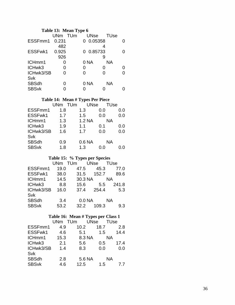
Table 13: Mean Type 6 UNm TUm UNse TUse
ESSFmm1 0.231482
0 0.053584
0
ESSFwk1 0.925926
0 0.857339
0
ICHmm1 0 0 NA NA ICHwk3 0 0 0 0ICHwk3/SBSvk
0 0 0 0
SBSdh 0 0 NA NA SBSvk 0 0 0 0
Table 14: Mean # Types Per Piece UNm TUm UNse TUse
ESSFmm1 1.8 1.3 0.0 0.0ESSFwk1 1.7 1.5 0.0 0.0ICHmm1 1.3 1.2 NA NA ICHwk3 1.9 1.1 0.1 0.0ICHwk3/SBSvk
1.6 1.7 0.0 0.0
SBSdh 0.9 0.6 NA NA SBSvk 1.8 1.3 0.0 0.0
Table 15: % Types per Species UNm TUm UNse TUse
ESSFmm1 19.0 47.5 45.3 77.0ESSFwk1 38.0 31.5 152.7 89.6ICHmm1 14.5 30.3 NA NA ICHwk3 8.8 15.6 5.5 241.8ICHwk3/SBSvk
16.0 37.4 254.4 5.3
SBSdh 3.4 0.0 NA NA SBSvk 53.2 32.2 109.3 9.3
Table 16: Mean # Types per Class 1 UNm TUm UNse TUse
ESSFmm1 4.9 10.2 18.7 2.8ESSFwk1 4.6 5.1 1.5 14.4ICHmm1 15.3 8.3 NA NA ICHwk3 2.1 5.6 0.5 17.4ICHwk3/SBSvk
1.4 8.3 0.0 0.0
SBSdh 2.8 5.6 NA NA SBSvk 4.6 12.5 1.5 7.7
36
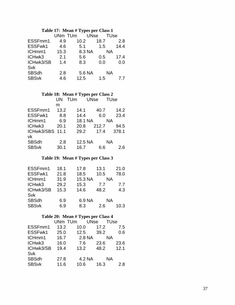
Table 17: Mean # Types per Class 1 UNm TUm UNse TUse
ESSFmm1 4.9 10.2 18.7 2.8ESSFwk1 4.6 5.1 1.5 14.4ICHmm1 15.3 8.3 NA NA ICHwk3 2.1 5.6 0.5 17.4ICHwk3/SBSvk
1.4 8.3 0.0 0.0
SBSdh 2.8 5.6 NA NA SBSvk 4.6 12.5 1.5 7.7
Table 18: Mean # Types per Class 2 UNm
TUm UNse TUse
ESSFmm1 13.2 14.1 40.7 14.2ESSFwk1 8.8 14.4 6.0 23.4ICHmm1 6.9 18.1 NA NA ICHwk3 20.1 20.8 212.7 94.5ICHwk3/SBSvk
11.1 29.2 17.4 378.1
SBSdh 2.8 12.5 NA NA SBSvk 30.1 16.7 6.6 2.6
Table 19: Mean # Types per Class 3 ESSFmm1 18.1 17.8 13.1 21.0ESSFwk1 21.8 18.5 10.5 78.0ICHmm1 31.9 15.3 NA NA ICHwk3 29.2 15.3 7.7 7.7ICHwk3/SBSvk
15.3 14.6 48.2 4.3
SBSdh 6.9 6.9 NA NA SBSvk 6.9 8.3 2.6 10.3
Table 20: Mean # Types per Class 4 UNm TUm UNse TUse
ESSFmm1 13.2 10.0 17.2 7.5ESSFwk1 25.0 12.5 39.2 0.6ICHmm1 16.7 2.8 NA NA ICHwk3 16.0 7.6 23.6 23.6ICHwk3/SBSvk
19.4 13.2 48.2 12.1
SBSdh 27.8 4.2 NA NA SBSvk 11.6 10.6 16.3 2.8
37
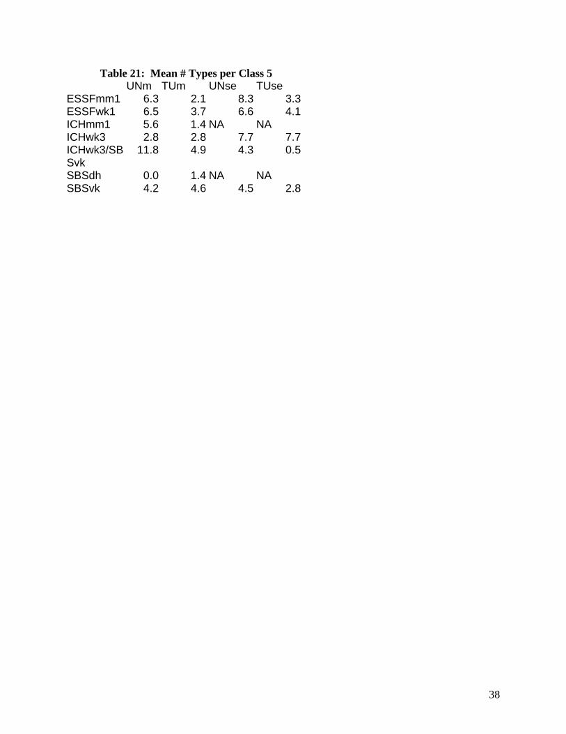
Table 21: Mean # Types per Class 5 UNm TUm UNse TUse
ESSFmm1 6.3 2.1 8.3 3.3ESSFwk1 6.5 3.7 6.6 4.1ICHmm1 5.6 1.4 NA NA ICHwk3 2.8 2.8 7.7 7.7ICHwk3/SBSvk
11.8 4.9 4.3 0.5
SBSdh 0.0 1.4 NA NA SBSvk 4.2 4.6 4.5 2.8
38
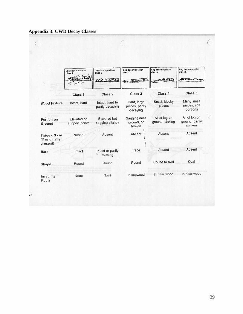
Appendix 3: CWD Decay Classes
39

Appendix 4; CWD Wildlife Types
40
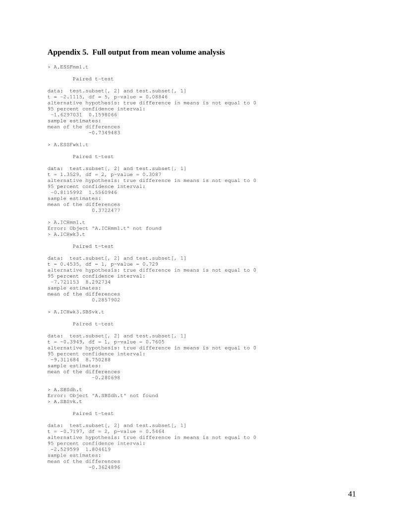
Appendix 5. Full output from mean volume analysis > A.ESSFmm1.t Paired t-test data: test.subset[, 2] and test.subset[, 1] t = -2.1115, df = 5, p-value = 0.08846 alternative hypothesis: true difference in means is not equal to 0 95 percent confidence interval: -1.6297031 0.1598066 sample estimates: mean of the differences -0.7349483 > A.ESSFwk1.t Paired t-test data: test.subset[, 2] and test.subset[, 1] t = 1.3529, df = 2, p-value = 0.3087 alternative hypothesis: true difference in means is not equal to 0 95 percent confidence interval: -0.8115992 1.5560946 sample estimates: mean of the differences 0.3722477 > A.ICHmm1.t Error: Object "A.ICHmm1.t" not found > A.ICHwk3.t Paired t-test data: test.subset[, 2] and test.subset[, 1] t = 0.4535, df = 1, p-value = 0.729 alternative hypothesis: true difference in means is not equal to 0 95 percent confidence interval: -7.721153 8.292734 sample estimates: mean of the differences 0.2857902 > A.ICHwk3.SBSvk.t Paired t-test data: test.subset[, 2] and test.subset[, 1] t = -0.3949, df = 1, p-value = 0.7605 alternative hypothesis: true difference in means is not equal to 0 95 percent confidence interval: -9.311684 8.750288 sample estimates: mean of the differences -0.280698 > A.SBSdh.t Error: Object "A.SBSdh.t" not found > A.SBSvk.t Paired t-test data: test.subset[, 2] and test.subset[, 1] t = -0.7197, df = 2, p-value = 0.5464 alternative hypothesis: true difference in means is not equal to 0 95 percent confidence interval: -2.529599 1.804619 sample estimates: mean of the differences -0.3624896
41
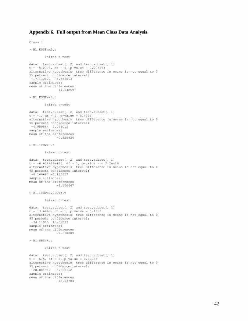
Appendix 6. Full output from Mean Class Data Analysis Class 1 > B1.ESSFmm1.t Paired t-test data: test.subset[, 2] and test.subset[, 1] t = -5.0379, df = 5, p-value = 0.003974 alternative hypothesis: true difference in means is not equal to 0 95 percent confidence interval: -17.130122 -5.555063 sample estimates: mean of the differences -11.34259 > B1.ESSFwk1.t Paired t-test data: test.subset[, 2] and test.subset[, 1] t = -1, df = 2, p-value = 0.4226 alternative hypothesis: true difference in means is not equal to 0 95 percent confidence interval: -4.909864 3.058012 sample estimates: mean of the differences -0.925926 > B1.ICHwk3.t Paired t-test data: test.subset[, 2] and test.subset[, 1] t = -6.634429e+15, df = 1, p-value = < 2.2e-16 alternative hypothesis: true difference in means is not equal to 0 95 percent confidence interval: -4.166667 -4.166667 sample estimates: mean of the differences -4.166667 > B1.ICHwk3.SBSvk.t Paired t-test data: test.subset[, 2] and test.subset[, 1] t = -3.6667, df = 1, p-value = 0.1695 alternative hypothesis: true difference in means is not equal to 0 95 percent confidence interval: -34.11015 18.83237 sample estimates: mean of the differences -7.638889 > B1.SBSvk.t Paired t-test data: test.subset[, 2] and test.subset[, 1] t = -6.5, df = 2, p-value = 0.02286 alternative hypothesis: true difference in means is not equal to 0 95 percent confidence interval: -20.004912 -4.069162 sample estimates: mean of the differences -12.03704
42
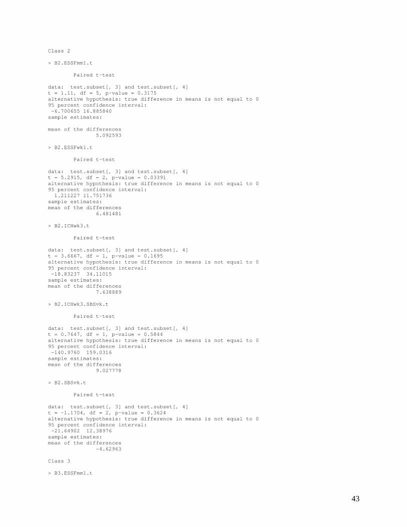
Class 2 > B2.ESSFmm1.t Paired t-test data: test.subset[, 3] and test.subset[, 4] t = 1.11, df = 5, p-value = 0.3175 alternative hypothesis: true difference in means is not equal to 0 95 percent confidence interval: -6.700655 16.885840 sample estimates: mean of the differences 5.092593 > B2.ESSFwk1.t Paired t-test data: test.subset[, 3] and test.subset[, 4] t = 5.2915, df = 2, p-value = 0.03391 alternative hypothesis: true difference in means is not equal to 0 95 percent confidence interval: 1.211227 11.751736 sample estimates: mean of the differences 6.481481 > B2.ICHwk3.t Paired t-test data: test.subset[, 3] and test.subset[, 4] t = 3.6667, df = 1, p-value = 0.1695 alternative hypothesis: true difference in means is not equal to 0 95 percent confidence interval: -18.83237 34.11015 sample estimates: mean of the differences 7.638889 > B2.ICHwk3.SBSvk.t Paired t-test data: test.subset[, 3] and test.subset[, 4] t = 0.7647, df = 1, p-value = 0.5844 alternative hypothesis: true difference in means is not equal to 0 95 percent confidence interval: -140.9760 159.0316 sample estimates: mean of the differences 9.027778 > B2.SBSvk.t Paired t-test data: test.subset[, 3] and test.subset[, 4] t = -1.1704, df = 2, p-value = 0.3624 alternative hypothesis: true difference in means is not equal to 0 95 percent confidence interval: -21.64902 12.38976 sample estimates: mean of the differences -4.62963 Class 3 > B3.ESSFmm1.t
43
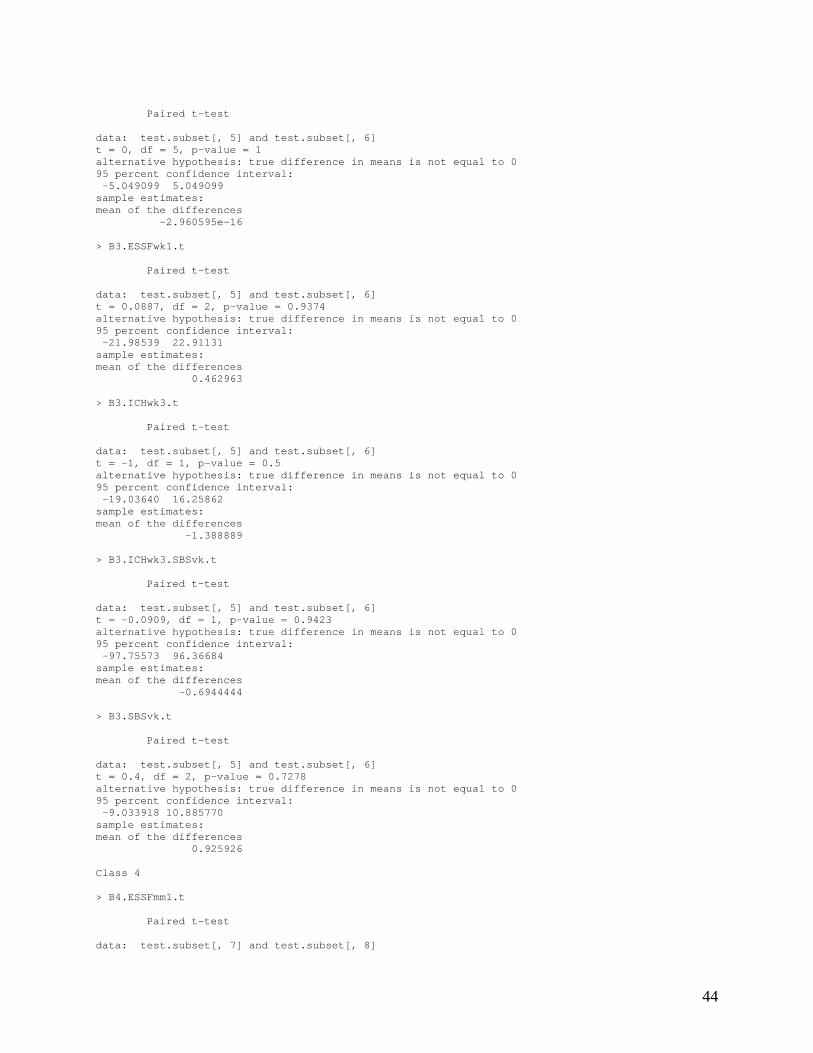
Paired t-test data: test.subset[, 5] and test.subset[, 6] t = 0, df = 5, p-value = 1 alternative hypothesis: true difference in means is not equal to 0 95 percent confidence interval: -5.049099 5.049099 sample estimates: mean of the differences -2.960595e-16 > B3.ESSFwk1.t Paired t-test data: test.subset[, 5] and test.subset[, 6] t = 0.0887, df = 2, p-value = 0.9374 alternative hypothesis: true difference in means is not equal to 0 95 percent confidence interval: -21.98539 22.91131 sample estimates: mean of the differences 0.462963 > B3.ICHwk3.t Paired t-test data: test.subset[, 5] and test.subset[, 6] t = -1, df = 1, p-value = 0.5 alternative hypothesis: true difference in means is not equal to 0 95 percent confidence interval: -19.03640 16.25862 sample estimates: mean of the differences -1.388889 > B3.ICHwk3.SBSvk.t Paired t-test data: test.subset[, 5] and test.subset[, 6] t = -0.0909, df = 1, p-value = 0.9423 alternative hypothesis: true difference in means is not equal to 0 95 percent confidence interval: -97.75573 96.36684 sample estimates: mean of the differences -0.6944444 > B3.SBSvk.t Paired t-test data: test.subset[, 5] and test.subset[, 6] t = 0.4, df = 2, p-value = 0.7278 alternative hypothesis: true difference in means is not equal to 0 95 percent confidence interval: -9.033918 10.885770 sample estimates: mean of the differences 0.925926 Class 4 > B4.ESSFmm1.t Paired t-test data: test.subset[, 7] and test.subset[, 8]
44
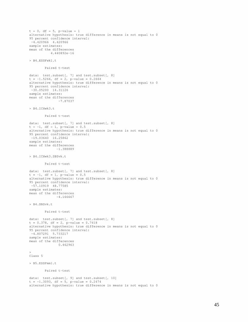
t = 0, df = 5, p-value = 1 alternative hypothesis: true difference in means is not equal to 0 95 percent confidence interval: -4.420966 4.420966 sample estimates: mean of the differences 4.440892e-16 > B4.ESSFwk1.t Paired t-test data: test.subset[, 7] and test.subset[, 8] t = -1.5266, df = 2, p-value = 0.2664 alternative hypothesis: true difference in means is not equal to 0 95 percent confidence interval: -30.05200 14.31126 sample estimates: mean of the differences -7.87037 > B4.ICHwk3.t Paired t-test data: test.subset[, 7] and test.subset[, 8] t = -1, df = 1, p-value = 0.5 alternative hypothesis: true difference in means is not equal to 0 95 percent confidence interval: -19.03640 16.25862 sample estimates: mean of the differences -1.388889 > B4.ICHwk3.SBSvk.t Paired t-test data: test.subset[, 7] and test.subset[, 8] t = -1, df = 1, p-value = 0.5 alternative hypothesis: true difference in means is not equal to 0 95 percent confidence interval: -57.10919 48.77585 sample estimates: mean of the differences -4.166667 > B4.SBSvk.t Paired t-test data: test.subset[, 7] and test.subset[, 8] t = 0.378, df = 2, p-value = 0.7418 alternative hypothesis: true difference in means is not equal to 0 95 percent confidence interval: -4.807291 5.733217 sample estimates: mean of the differences 0.462963 > Class 5 > B5.ESSFmm1.t Paired t-test data: test.subset[, 9] and test.subset[, 10] t = -1.3093, df = 5, p-value = 0.2474 alternative hypothesis: true difference in means is not equal to 0
45

95 percent confidence interval: -8.231428 2.675873 sample estimates: mean of the differences -2.777778 > B5.ESSFwk1.t Paired t-test data: test.subset[, 9] and test.subset[, 10] t = -2, df = 2, p-value = 0.1835 alternative hypothesis: true difference in means is not equal to 0 95 percent confidence interval: -11.671579 4.264172 sample estimates: mean of the differences -3.703704 > B5.ICHwk3.t Paired t-test data: test.subset[, 9] and test.subset[, 10] t = 0, df = 1, p-value = 1 alternative hypothesis: true difference in means is not equal to 0 95 percent confidence interval: -35.29501 35.29501 sample estimates: mean of the differences 0 > B5.ICHwk3.SBSvk.t Paired t-test data: test.subset[, 9] and test.subset[, 10] t = -3, df = 1, p-value = 0.2048 alternative hypothesis: true difference in means is not equal to 0 95 percent confidence interval: -32.72126 20.22126 sample estimates: mean of the differences -6.25 > B5.SBSvk.t Paired t-test data: test.subset[, 9] and test.subset[, 10] t = 0.2294, df = 2, p-value = 0.8399 alternative hypothesis: true difference in means is not equal to 0 95 percent confidence interval: -16.43966 18.29151 sample estimates: mean of the differences 0.925926
46
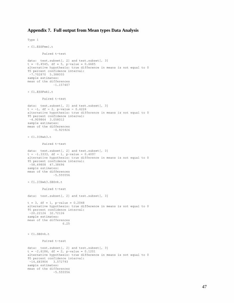
Appendix 7. Full output from Mean types Data Analysis Type 1 > C1.ESSFmm1.t Paired t-test data: test.subset[, 2] and test.subset[, 3] t = -0.4545, df = 5, p-value = 0.6685 alternative hypothesis: true difference in means is not equal to 0 95 percent confidence interval: -7.702870 5.388055 sample estimates: mean of the differences -1.157407 > C1.ESSFwk1.t Paired t-test data: test.subset[, 2] and test.subset[, 3] t = -1, df = 2, p-value = 0.4226 alternative hypothesis: true difference in means is not equal to 0 95 percent confidence interval: -4.909864 3.058012 sample estimates: mean of the differences -0.925926 > C1.ICHwk3.t Paired t-test data: test.subset[, 2] and test.subset[, 3] t = -1.3333, df = 1, p-value = 0.4097 alternative hypothesis: true difference in means is not equal to 0 95 percent confidence interval: -58.49808 47.38696 sample estimates: mean of the differences -5.555556 > C1.ICHwk3.SBSvk.t Paired t-test data: test.subset[, 2] and test.subset[, 3] t = 3, df = 1, p-value = 0.2048 alternative hypothesis: true difference in means is not equal to 0 95 percent confidence interval: -20.22126 32.72126 sample estimates: mean of the differences 6.25 > C1.SBSvk.t Paired t-test data: test.subset[, 2] and test.subset[, 3] t = -2.6186, df = 2, p-value = 0.1201 alternative hypothesis: true difference in means is not equal to 0 95 percent confidence interval: -14.683904 3.572793 sample estimates: mean of the differences -5.555556
47
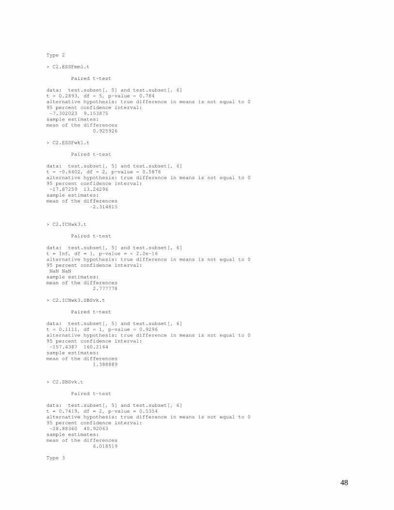
Type 2 > C2.ESSFmm1.t Paired t-test data: test.subset[, 5] and test.subset[, 6] t = 0.2893, df = 5, p-value = 0.784 alternative hypothesis: true difference in means is not equal to 0 95 percent confidence interval: -7.302023 9.153875 sample estimates: mean of the differences 0.925926 > C2.ESSFwk1.t Paired t-test data: test.subset[, 5] and test.subset[, 6] t = -0.6402, df = 2, p-value = 0.5876 alternative hypothesis: true difference in means is not equal to 0 95 percent confidence interval: -17.87259 13.24296 sample estimates: mean of the differences -2.314815 > C2.ICHwk3.t Paired t-test data: test.subset[, 5] and test.subset[, 6] t = Inf, df = 1, p-value = < 2.2e-16 alternative hypothesis: true difference in means is not equal to 0 95 percent confidence interval: NaN NaN sample estimates: mean of the differences 2.777778 > C2.ICHwk3.SBSvk.t Paired t-test data: test.subset[, 5] and test.subset[, 6] t = 0.1111, df = 1, p-value = 0.9296 alternative hypothesis: true difference in means is not equal to 0 95 percent confidence interval: -157.4387 160.2164 sample estimates: mean of the differences 1.388889 > C2.SBSvk.t Paired t-test data: test.subset[, 5] and test.subset[, 6] t = 0.7419, df = 2, p-value = 0.5354 alternative hypothesis: true difference in means is not equal to 0 95 percent confidence interval: -28.88360 40.92063 sample estimates: mean of the differences 6.018519 Type 3
48
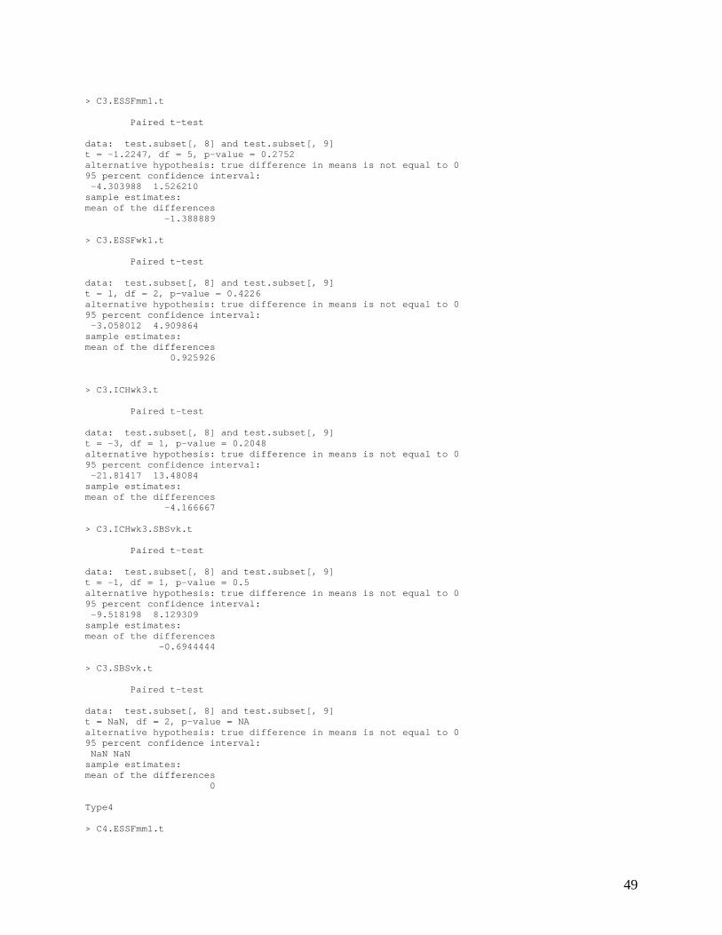
> C3.ESSFmm1.t Paired t-test data: test.subset[, 8] and test.subset[, 9] t = -1.2247, df = 5, p-value = 0.2752 alternative hypothesis: true difference in means is not equal to 0 95 percent confidence interval: -4.303988 1.526210 sample estimates: mean of the differences -1.388889 > C3.ESSFwk1.t Paired t-test data: test.subset[, 8] and test.subset[, 9] t = 1, df = 2, p-value = 0.4226 alternative hypothesis: true difference in means is not equal to 0 95 percent confidence interval: -3.058012 4.909864 sample estimates: mean of the differences 0.925926 > C3.ICHwk3.t Paired t-test data: test.subset[, 8] and test.subset[, 9] t = -3, df = 1, p-value = 0.2048 alternative hypothesis: true difference in means is not equal to 0 95 percent confidence interval: -21.81417 13.48084 sample estimates: mean of the differences -4.166667 > C3.ICHwk3.SBSvk.t Paired t-test data: test.subset[, 8] and test.subset[, 9] t = -1, df = 1, p-value = 0.5 alternative hypothesis: true difference in means is not equal to 0 95 percent confidence interval: -9.518198 8.129309 sample estimates: mean of the differences -0.6944444 > C3.SBSvk.t Paired t-test data: test.subset[, 8] and test.subset[, 9] t = NaN, df = 2, p-value = NA alternative hypothesis: true difference in means is not equal to 0 95 percent confidence interval: NaN NaN sample estimates: mean of the differences 0 Type4 > C4.ESSFmm1.t
49
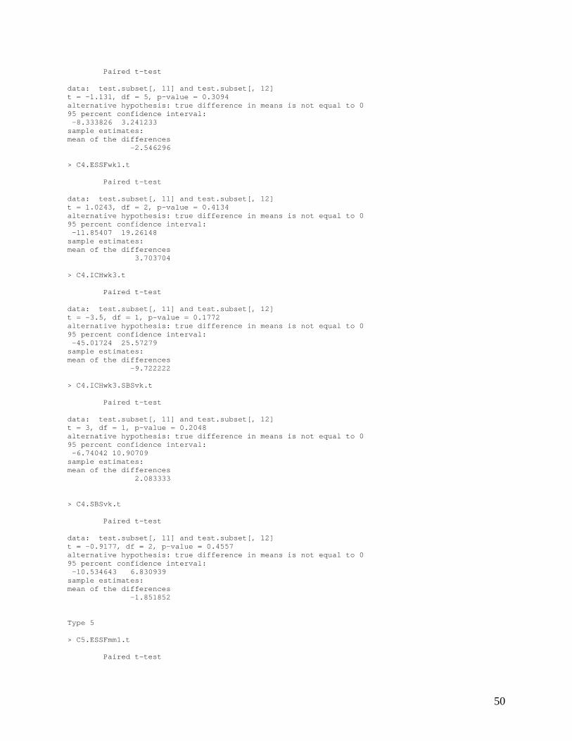
Paired t-test data: test.subset[, 11] and test.subset[, 12] t = -1.131, df = 5, p-value = 0.3094 alternative hypothesis: true difference in means is not equal to 0 95 percent confidence interval: -8.333826 3.241233 sample estimates: mean of the differences -2.546296 > C4.ESSFwk1.t Paired t-test data: test.subset[, 11] and test.subset[, 12] t = 1.0243, df = 2, p-value = 0.4134 alternative hypothesis: true difference in means is not equal to 0 95 percent confidence interval: -11.85407 19.26148 sample estimates: mean of the differences 3.703704 > C4.ICHwk3.t Paired t-test data: test.subset[, 11] and test.subset[, 12] t = -3.5, df = 1, p-value = 0.1772 alternative hypothesis: true difference in means is not equal to 0 95 percent confidence interval: -45.01724 25.57279 sample estimates: mean of the differences -9.722222 > C4.ICHwk3.SBSvk.t Paired t-test data: test.subset[, 11] and test.subset[, 12] t = 3, df = 1, p-value = 0.2048 alternative hypothesis: true difference in means is not equal to 0 95 percent confidence interval: -6.74042 10.90709 sample estimates: mean of the differences 2.083333 > C4.SBSvk.t Paired t-test data: test.subset[, 11] and test.subset[, 12] t = -0.9177, df = 2, p-value = 0.4557 alternative hypothesis: true difference in means is not equal to 0 95 percent confidence interval: -10.534643 6.830939 sample estimates: mean of the differences -1.851852 Type 5 > C5.ESSFmm1.t Paired t-test
50
data: test.subset[, 14] and test.subset[, 15] t = 1.1937, df = 5, p-value = 0.2861 alternative hypothesis: true difference in means is not equal to 0 95 percent confidence interval: -3.470965 9.489483 sample estimates: mean of the differences 3.009259 > C5.ESSFwk1.t Paired t-test data: test.subset[, 14] and test.subset[, 15] t = -10, df = 2, p-value = 0.009852 alternative hypothesis: true difference in means is not equal to 0 95 percent confidence interval: -6.621598 -2.637661 sample estimates: mean of the differences -4.62963 > C5.ICHwk3.t Paired t-test data: test.subset[, 14] and test.subset[, 15] t = -0.3333, df = 1, p-value = 0.7952 alternative hypothesis: true difference in means is not equal to 0 95 percent confidence interval: -54.33141 51.55363 sample estimates: mean of the differences -1.388889 > C5.ICHwk3.SBSvk.t Paired t-test data: test.subset[, 14] and test.subset[, 15] t = 0.4118, df = 1, p-value = 0.7513 alternative hypothesis: true difference in means is not equal to 0 95 percent confidence interval: -145.1427 154.8649 sample estimates: mean of the differences 4.861111 > C5.SBSvk.t Paired t-test data: test.subset[, 14] and test.subset[, 15] t = -0.8963, df = 2, p-value = 0.4647 alternative hypothesis: true difference in means is not equal to 0 95 percent confidence interval: -18.79851 12.31703 sample estimates: mean of the differences -3.240741 Type 6 > C6.ESSFmm1.t Paired t-test data: test.subset[, 17] and test.subset[, 18]
51
t = -1, df = 5, p-value = 0.3632 alternative hypothesis: true difference in means is not equal to 0 95 percent confidence interval: -0.8265235 0.3635606 sample estimates: mean of the differences -0.2314815 > C6.ESSFwk1.t Paired t-test data: test.subset[, 17] and test.subset[, 18] t = -1, df = 2, p-value = 0.4226 alternative hypothesis: true difference in means is not equal to 0 95 percent confidence interval: -4.909864 3.058012 sample estimates: mean of the differences -0.925926 > C6.ICHwk3.t Paired t-test data: test.subset[, 17] and test.subset[, 18] t = NaN, df = 1, p-value = NA alternative hypothesis: true difference in means is not equal to 0 95 percent confidence interval: NaN NaN sample estimates: mean of the differences 0 > C6.ICHwk3.SBSvk.t Paired t-test data: test.subset[, 17] and test.subset[, 18] t = NaN, df = 1, p-value = NA alternative hypothesis: true difference in means is not equal to 0 95 percent confidence interval: NaN NaN sample estimates: mean of the differences 0 > C6.SBSvk.t Paired t-test data: test.subset[, 17] and test.subset[, 18] t = NaN, df = 2, p-value = NA alternative hypothesis: true difference in means is not equal to 0 95 percent confidence interval: NaN NaN sample estimates: mean of the differences 0 >
52
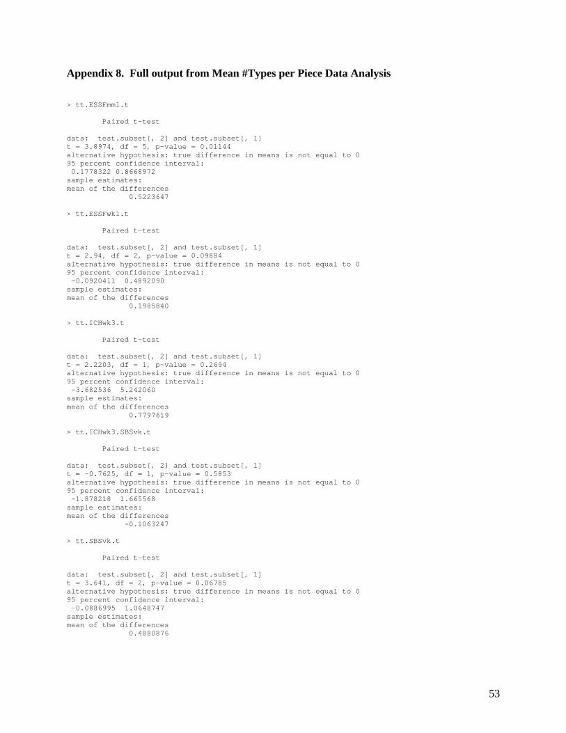
Appendix 8. Full output from Mean #Types per Piece Data Analysis > tt.ESSFmm1.t Paired t-test data: test.subset[, 2] and test.subset[, 1] t = 3.8974, df = 5, p-value = 0.01144 alternative hypothesis: true difference in means is not equal to 0 95 percent confidence interval: 0.1778322 0.8668972 sample estimates: mean of the differences 0.5223647 > tt.ESSFwk1.t Paired t-test data: test.subset[, 2] and test.subset[, 1] t = 2.94, df = 2, p-value = 0.09884 alternative hypothesis: true difference in means is not equal to 0 95 percent confidence interval: -0.0920411 0.4892090 sample estimates: mean of the differences 0.1985840 > tt.ICHwk3.t Paired t-test data: test.subset[, 2] and test.subset[, 1] t = 2.2203, df = 1, p-value = 0.2694 alternative hypothesis: true difference in means is not equal to 0 95 percent confidence interval: -3.682536 5.242060 sample estimates: mean of the differences 0.7797619 > tt.ICHwk3.SBSvk.t Paired t-test data: test.subset[, 2] and test.subset[, 1] t = -0.7625, df = 1, p-value = 0.5853 alternative hypothesis: true difference in means is not equal to 0 95 percent confidence interval: -1.878218 1.665568 sample estimates: mean of the differences -0.1063247 > tt.SBSvk.t Paired t-test data: test.subset[, 2] and test.subset[, 1] t = 3.641, df = 2, p-value = 0.06785 alternative hypothesis: true difference in means is not equal to 0 95 percent confidence interval: -0.0886995 1.0648747 sample estimates: mean of the differences 0.4880876
53

Appendix 9. Output from % Types by Species Data Analysis Species =Bi > E1.ESSFmm1.t Paired t-test data: test.subset[, i] and test.subset[, i + 16] t = 2.6004, df = 5, p-value = 0.04822 alternative hypothesis: true difference in means is not equal to 0 95 percent confidence interval: 0.3271596 56.6728404 sample estimates: mean of the differences 28.5 > E1.ESSFwk1.t Paired t-test data: test.subset[, i] and test.subset[, i + 16] t = -0.6611, df = 2, p-value = 0.5765 alternative hypothesis: true difference in means is not equal to 0 95 percent confidence interval: -48.80407 35.80407 sample estimates: mean of the differences -6.5 > E1.ICHwk3.t Paired t-test data: test.subset[, i] and test.subset[, i + 16] t = 0.5152, df = 1, p-value = 0.6972 alternative hypothesis: true difference in means is not equal to 0 95 percent confidence interval: -160.9219 174.5219 sample estimates: mean of the differences 6.8 > E1.ICHwk3.SBSvk.t Paired t-test data: test.subset[, i] and test.subset[, i + 16] t = 1.1753, df = 1, p-value = 0.4488 alternative hypothesis: true difference in means is not equal to 0 95 percent confidence interval: -210.4382 253.3382 sample estimates: mean of the differences 21.45 > E1.SBSvk.t Paired t-test data: test.subset[, i] and test.subset[, i + 16] t = -2.4516, df = 2, p-value = 0.1338 alternative hypothesis: true difference in means is not equal to 0 95 percent confidence interval: -58.03973 15.90639 sample estimates: mean of the differences -21.06667 Species =Cw
54
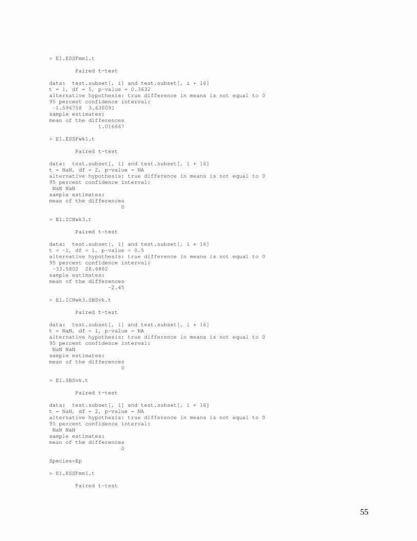
> E1.ESSFmm1.t Paired t-test data: test.subset[, i] and test.subset[, i + 16] t = 1, df = 5, p-value = 0.3632 alternative hypothesis: true difference in means is not equal to 0 95 percent confidence interval: -1.596758 3.630091 sample estimates: mean of the differences 1.016667 > E1.ESSFwk1.t Paired t-test data: test.subset[, i] and test.subset[, i + 16] t = NaN, df = 2, p-value = NA alternative hypothesis: true difference in means is not equal to 0 95 percent confidence interval: NaN NaN sample estimates: mean of the differences 0 > E1.ICHwk3.t Paired t-test data: test.subset[, i] and test.subset[, i + 16] t = -1, df = 1, p-value = 0.5 alternative hypothesis: true difference in means is not equal to 0 95 percent confidence interval: -33.5802 28.6802 sample estimates: mean of the differences -2.45 > E1.ICHwk3.SBSvk.t Paired t-test data: test.subset[, i] and test.subset[, i + 16] t = NaN, df = 1, p-value = NA alternative hypothesis: true difference in means is not equal to 0 95 percent confidence interval: NaN NaN sample estimates: mean of the differences 0 > E1.SBSvk.t Paired t-test data: test.subset[, i] and test.subset[, i + 16] t = NaN, df = 2, p-value = NA alternative hypothesis: true difference in means is not equal to 0 95 percent confidence interval: NaN NaN sample estimates: mean of the differences 0 Species=Ep > E1.ESSFmm1.t Paired t-test
55
data: test.subset[, i] and test.subset[, i + 16] t = -1, df = 5, p-value = 0.3632 alternative hypothesis: true difference in means is not equal to 0 95 percent confidence interval: -1.7852908 0.7852908 sample estimates: mean of the differences -0.5 > E1.ESSFwk1.t Paired t-test data: test.subset[, i] and test.subset[, i + 16] t = NaN, df = 2, p-value = NA alternative hypothesis: true difference in means is not equal to 0 95 percent confidence interval: NaN NaN sample estimates: mean of the differences 0 > E1.ICHwk3.t Paired t-test data: test.subset[, i] and test.subset[, i + 16] t = NaN, df = 1, p-value = NA alternative hypothesis: true difference in means is not equal to 0 95 percent confidence interval: NaN NaN sample estimates: mean of the differences 0 > E1.ICHwk3.SBSvk.t Paired t-test data: test.subset[, i] and test.subset[, i + 16] t = NaN, df = 1, p-value = NA alternative hypothesis: true difference in means is not equal to 0 95 percent confidence interval: NaN NaN sample estimates: mean of the differences 0 > E1.SBSvk.t Paired t-test data: test.subset[, i] and test.subset[, i + 16] t = NaN, df = 2, p-value = NA alternative hypothesis: true difference in means is not equal to 0 95 percent confidence interval: NaN NaN sample estimates: mean of the differences 0 Species= Fd > E1.ESSFmm1.t Paired t-test data: test.subset[, i] and test.subset[, i + 16] t = NaN, df = 5, p-value = NA
56
alternative hypothesis: true difference in means is not equal to 0 95 percent confidence interval: NaN NaN sample estimates: mean of the differences 0 > E1.ESSFwk1.t Paired t-test data: test.subset[, i] and test.subset[, i + 16] t = NaN, df = 2, p-value = NA alternative hypothesis: true difference in means is not equal to 0 95 percent confidence interval: NaN NaN sample estimates: mean of the differences 0 > E1.ICHwk3.t Paired t-test data: test.subset[, i] and test.subset[, i + 16] t = NaN, df = 1, p-value = NA alternative hypothesis: true difference in means is not equal to 0 95 percent confidence interval: NaN NaN sample estimates: mean of the differences 0 > E1.ICHwk3.SBSvk.t Paired t-test data: test.subset[, i] and test.subset[, i + 16] t = 1, df = 1, p-value = 0.5 alternative hypothesis: true difference in means is not equal to 0 95 percent confidence interval: -8.779654 10.279654 sample estimates: mean of the differences 0.75 > E1.SBSvk.t Paired t-test data: test.subset[, i] and test.subset[, i + 16] t = NaN, df = 2, p-value = NA alternative hypothesis: true difference in means is not equal to 0 95 percent confidence interval: NaN NaN sample estimates: mean of the differences 0 Species= Hw > E1.ESSFmm1.t Paired t-test data: test.subset[, i] and test.subset[, i + 16] t = NaN, df = 5, p-value = NA alternative hypothesis: true difference in means is not equal to 0 95 percent confidence interval: NaN NaN sample estimates:
57
mean of the differences 0 > E1.ESSFwk1.t Paired t-test data: test.subset[, i] and test.subset[, i + 16] t = NaN, df = 2, p-value = NA alternative hypothesis: true difference in means is not equal to 0 95 percent confidence interval: NaN NaN sample estimates: mean of the differences 0 > E1.ICHwk3.t Paired t-test data: test.subset[, i] and test.subset[, i + 16] t = 0.0158, df = 1, p-value = 0.99 alternative hypothesis: true difference in means is not equal to 0 95 percent confidence interval: -201.1433 201.6433 sample estimates: mean of the differences 0.25 > E1.ICHwk3.SBSvk.t Paired t-test data: test.subset[, i] and test.subset[, i + 16] t = -1, df = 1, p-value = 0.5 alternative hypothesis: true difference in means is not equal to 0 95 percent confidence interval: -123.3558 105.3558 sample estimates: mean of the differences -9 > E1.SBSvk.t Paired t-test data: test.subset[, i] and test.subset[, i + 16] t = 2.3275, df = 2, p-value = 0.1454 alternative hypothesis: true difference in means is not equal to 0 95 percent confidence interval: -14.34192 48.14192 sample estimates: mean of the differences 16.9 Species= S1 > E1.ESSFmm1.t Paired t-test data: test.subset[, i] and test.subset[, i + 16] t = -1.8462, df = 5, p-value = 0.1242 alternative hypothesis: true difference in means is not equal to 0 95 percent confidence interval: -39.713518 6.513518 sample estimates: mean of the differences -16.6
58
> E1.ESSFwk1.t Paired t-test data: test.subset[, i] and test.subset[, i + 16] t = -0.5684, df = 2, p-value = 0.6271 alternative hypothesis: true difference in means is not equal to 0 95 percent confidence interval: -29.42356 22.55689 sample estimates: mean of the differences -3.433333 > E1.ICHwk3.t Paired t-test data: test.subset[, i] and test.subset[, i + 16] t = -0.1698, df = 1, p-value = 0.893 alternative hypothesis: true difference in means is not equal to 0 95 percent confidence interval: -34.12144 33.22144 sample estimates: mean of the differences -0.45 > E1.ICHwk3.SBSvk.t Paired t-test data: test.subset[, i] and test.subset[, i + 16] t = 0.009, df = 1, p-value = 0.9943 alternative hypothesis: true difference in means is not equal to 0 95 percent confidence interval: -211.4083 211.7083 sample estimates: mean of the differences 0.15 > E1.SBSvk.t Paired t-test data: test.subset[, i] and test.subset[, i + 16] t = 1.6928, df = 2, p-value = 0.2326 alternative hypothesis: true difference in means is not equal to 0 95 percent confidence interval: -16.03361 36.83361 sample estimates: mean of the differences 10.4 Species =U > E1.ESSFmm1.t Paired t-test data: test.subset[, i] and test.subset[, i + 16] t = -1.1633, df = 5, p-value = 0.2972 alternative hypothesis: true difference in means is not equal to 0 95 percent confidence interval: -37.82215 14.25548 sample estimates: mean of the differences -11.78333 > E1.ESSFwk1.t Paired t-test
59
data: test.subset[, i] and test.subset[, i + 16] t = 0.6396, df = 2, p-value = 0.5879 alternative hypothesis: true difference in means is not equal to 0 95 percent confidence interval: -37.98812 51.25479 sample estimates: mean of the differences 6.633333 > E1.ICHwk3.t Paired t-test data: test.subset[, i] and test.subset[, i + 16] t = -1.7917, df = 1, p-value = 0.3241 alternative hypothesis: true difference in means is not equal to 0 95 percent confidence interval: -34.79489 26.19489 sample estimates: mean of the differences -4.3 > E1.ICHwk3.SBSvk.t Paired t-test data: test.subset[, i] and test.subset[, i + 16] t = -1.9778, df = 1, p-value = 0.298 alternative hypothesis: true difference in means is not equal to 0 95 percent confidence interval: -99.11688 72.41688 sample estimates: mean of the differences -13.35 > E1.SBSvk.t Paired t-test data: test.subset[, i] and test.subset[, i + 16] t = -1.2146, df = 2, p-value = 0.3485 alternative hypothesis: true difference in means is not equal to 0 95 percent confidence interval: -28.46648 15.93315 sample estimates: mean of the differences -6.266667 Species = Totals> > E1.ESSFmm1.t Paired t-test data: test.subset[, i] and test.subset[, i + 16] t = -0.1405, df = 5, p-value = 0.8938 alternative hypothesis: true difference in means is not equal to 0 95 percent confidence interval: -19.29753 17.29753 sample estimates: mean of the differences -1 > E1.ESSFwk1.t Paired t-test data: test.subset[, i] and test.subset[, i + 16] t = -0.9686, df = 2, p-value = 0.4349
60
alternative hypothesis: true difference in means is not equal to 0 95 percent confidence interval: -48.97841 30.97841 sample estimates: mean of the differences -9 > E1.ICHwk3.t Paired t-test data: test.subset[, i] and test.subset[, i + 16] t = -3.5714, df = 1, p-value = 0.1738 alternative hypothesis: true difference in means is not equal to 0 95 percent confidence interval: -56.97172 31.97172 sample estimates: mean of the differences -12.5 > E1.ICHwk3.SBSvk.t Paired t-test data: test.subset[, i] and test.subset[, i + 16] t = 0.5, df = 1, p-value = 0.7048 alternative hypothesis: true difference in means is not equal to 0 95 percent confidence interval: -244.1241 264.1241 sample estimates: mean of the differences 10 > E1.SBSvk.t Paired t-test data: test.subset[, i] and test.subset[, i + 16] t = -0.4981, df = 2, p-value = 0.6678 alternative hypothesis: true difference in means is not equal to 0 95 percent confidence interval: -32.12505 25.45838 sample estimates: mean of the differences -3.333333
Appendix 10 – Output From Mean # Types per class Data Analysis > F1.ESSFmm1.t Paired t-test data: test.subset[, 2] and test.subset[, 1] t = -1.9425, df = 5, p-value = 0.1097 alternative hypothesis: true difference in means is not equal to 0 95 percent confidence interval: -12.369734 1.721586 sample estimates: mean of the differences -5.324074 > F1.ESSFwk1.t Paired t-test
61
data: test.subset[, 2] and test.subset[, 1] t = -0.117, df = 2, p-value = 0.9175 alternative hypothesis: true difference in means is not equal to 0 95 percent confidence interval: -17.48235 16.55643 sample estimates: mean of the differences -0.462963 > F1.ICHmm1.t Error: Object "F1.ICHmm1.t" not found > F1.ICHwk3.t Paired t-test data: test.subset[, 2] and test.subset[, 1] t = -1, df = 1, p-value = 0.5 alternative hypothesis: true difference in means is not equal to 0 95 percent confidence interval: -47.59099 40.64654 sample estimates: mean of the differences -3.472222 > F1.ICHwk3.SBSvk.t Paired t-test data: test.subset[, 2] and test.subset[, 1] t = -Inf, df = 1, p-value = < 2.2e-16 alternative hypothesis: true difference in means is not equal to 0 95 percent confidence interval: NaN NaN sample estimates: mean of the differences -6.944444 > F1.SBSdh.t Error: Object "F1.SBSdh.t" not found > F1.SBSvk.t Paired t-test data: test.subset[, 2] and test.subset[, 1] t = -2.7948, df = 2, p-value = 0.1077 alternative hypothesis: true difference in means is not equal to 0 95 percent confidence interval: -19.987044 4.246303 sample estimates: mean of the differences -7.87037 > > #Testing class 2 means > test.subset <- TabF3[rownames(TabF3)=="ESSFmm1",] > F2.ESSFmm1.t<-t.test(test.subset[,3],test.subset[,4], paired=T)
62
> test.subset <- TabF3[rownames(TabF3)=="ESSFwk1",] > F2.ESSFwk1.t <-t.test(test.subset[,3],test.subset[,4], paired=T) > test.subset <- TabF3[rownames(TabF3)=="ICHmm1",] > F2.ICHmm1.t <-t.test(test.subset[,3],test.subset[,4], paired=T) Error in test.subset[, 3] : incorrect number of dimensions > test.subset <- TabF3[rownames(TabF3)=="ICHwk3",] > F2.ICHwk3.t <-t.test(test.subset[,3],test.subset[,4], paired=T) > test.subset <- TabF3[rownames(TabF3)=="ICHwk3/SBSvk",] > F2.ICHwk3.SBSvk.t <-t.test(test.subset[,3],test.subset[,4], paired=T) > test.subset <- TabF3[rownames(TabF3)=="SBSdh",] > F2.SBSdh.t <-t.test(test.subset[,3],test.subset[,4], paired=T) Error in test.subset[, 3] : incorrect number of dimensions > test.subset <- TabF3[rownames(TabF3)=="SBSvk",] > F2.SBSvk.t <- t.test(test.subset[,3],test.subset[,4], paired=T) > > > F2.ESSFmm1.t Paired t-test data: test.subset[, 3] and test.subset[, 4] t = 0.1118, df = 5, p-value = 0.9154 alternative hypothesis: true difference in means is not equal to 0 95 percent confidence interval: -20.36960 22.22145 sample estimates: mean of the differences 0.925926 > F2.ESSFwk1.t Paired t-test data: test.subset[, 3] and test.subset[, 4] t = 1.139, df = 2, p-value = 0.3727 alternative hypothesis: true difference in means is not equal to 0 95 percent confidence interval: -15.43114 26.54225 sample estimates: mean of the differences 5.555556 > F2.ICHmm1.t Error: Object "F2.ICHmm1.t" not found > F2.ICHwk3.t Paired t-test data: test.subset[, 3] and test.subset[, 4] t = 0.1429, df = 1, p-value = 0.9097 alternative hypothesis: true difference in means is not equal to 0 95 percent confidence interval: -61.07183 62.46072 sample estimates: mean of the differences 0.6944444
63

> F2.ICHwk3.SBSvk.t Paired t-test data: test.subset[, 3] and test.subset[, 4] t = 0.7647, df = 1, p-value = 0.5844 alternative hypothesis: true difference in means is not equal to 0 95 percent confidence interval: -281.9521 318.0632 sample estimates: mean of the differences 18.05556 > F2.SBSdh.t Error: Object "F2.SBSdh.t" not found > F2.SBSvk.t Paired t-test data: test.subset[, 3] and test.subset[, 4] t = -4.1429, df = 2, p-value = 0.05362 alternative hypothesis: true difference in means is not equal to 0 95 percent confidence interval: -27.3697079 0.5178561 sample estimates: mean of the differences -13.42593 > > > #Testing class 3 means > test.subset <- TabF3[rownames(TabF3)=="ESSFmm1",] > F3.ESSFmm1.t<-t.test(test.subset[,5],test.subset[,6], paired=T) > test.subset <- TabF3[rownames(TabF3)=="ESSFwk1",] > F3.ESSFwk1.t <-t.test(test.subset[,5],test.subset[,6], paired=T) > test.subset <- TabF3[rownames(TabF3)=="ICHmm1",] > F3.ICHmm1.t <-t.test(test.subset[,5],test.subset[,6], paired=T) Error in test.subset[, 5] : incorrect number of dimensions > test.subset <- TabF3[rownames(TabF3)=="ICHwk3",] > F3.ICHwk3.t <-t.test(test.subset[,5],test.subset[,6], paired=T) > test.subset <- TabF3[rownames(TabF3)=="ICHwk3/SBSvk",] > F3.ICHwk3.SBSvk.t <-t.test(test.subset[,5],test.subset[,6], paired=T) > test.subset <- TabF3[rownames(TabF3)=="SBSdh",] > F3.SBSdh.t <-t.test(test.subset[,5],test.subset[,6], paired=T) Error in test.subset[, 5] : incorrect number of dimensions > test.subset <- TabF3[rownames(TabF3)=="SBSvk",] > F3.SBSvk.t <- t.test(test.subset[,5],test.subset[,6], paired=T) > > > F3.ESSFmm1.t Paired t-test data: test.subset[, 5] and test.subset[, 6] t = -0.0661, df = 5, p-value = 0.9499 alternative hypothesis: true difference in means is not equal to 0 95 percent confidence interval:
64

-9.236102 8.773139 sample estimates: mean of the differences -0.2314815 > F3.ESSFwk1.t Paired t-test data: test.subset[, 5] and test.subset[, 6] t = -0.3212, df = 2, p-value = 0.7785 alternative hypothesis: true difference in means is not equal to 0 95 percent confidence interval: -46.65470 40.17321 sample estimates: mean of the differences -3.240741 > F3.ICHmm1.t Error: Object "F3.ICHmm1.t" not found > F3.ICHwk3.t Paired t-test data: test.subset[, 5] and test.subset[, 6] t = -2.5, df = 1, p-value = 0.2422 alternative hypothesis: true difference in means is not equal to 0 95 percent confidence interval: -84.47892 56.70114 sample estimates: mean of the differences -13.88889 > F3.ICHwk3.SBSvk.t Paired t-test data: test.subset[, 5] and test.subset[, 6] t = -0.0769, df = 1, p-value = 0.9511 alternative hypothesis: true difference in means is not equal to 0 95 percent confidence interval: -115.4032 114.0143 sample estimates: mean of the differences -0.6944444 > F3.SBSdh.t Error: Object "F3.SBSdh.t" not found > F3.SBSvk.t Paired t-test data: test.subset[, 5] and test.subset[, 6] t = 0.2887, df = 2, p-value = 0.8 alternative hypothesis: true difference in means is not equal to 0 95 percent confidence interval:
65
-19.31226 22.09004 sample estimates: mean of the differences 1.388889 > > > #Testing class 4 means > test.subset <- TabF3[rownames(TabF3)=="ESSFmm1",] > F4.ESSFmm1.t<-t.test(test.subset[,7],test.subset[,8], paired=T) > test.subset <- TabF3[rownames(TabF3)=="ESSFwk1",] > F4.ESSFwk1.t <-t.test(test.subset[,7],test.subset[,8], paired=T) > test.subset <- TabF3[rownames(TabF3)=="ICHmm1",] > F4.ICHmm1.t <-t.test(test.subset[,7],test.subset[,8], paired=T) Error in test.subset[, 7] : incorrect number of dimensions > test.subset <- TabF3[rownames(TabF3)=="ICHwk3",] > F4.ICHwk3.t <-t.test(test.subset[,7],test.subset[,8], paired=T) > test.subset <- TabF3[rownames(TabF3)=="ICHwk3/SBSvk",] > F4.ICHwk3.SBSvk.t <-t.test(test.subset[,7],test.subset[,8], paired=T) > test.subset <- TabF3[rownames(TabF3)=="SBSdh",] > F4.SBSdh.t <-t.test(test.subset[,7],test.subset[,8], paired=T) Error in test.subset[, 7] : incorrect number of dimensions > test.subset <- TabF3[rownames(TabF3)=="SBSvk",] > F4.SBSvk.t <- t.test(test.subset[,7],test.subset[,8], paired=T) > > > F4.ESSFmm1.t Paired t-test data: test.subset[, 7] and test.subset[, 8] t = -0.859, df = 5, p-value = 0.4296 alternative hypothesis: true difference in means is not equal to 0 95 percent confidence interval: -12.938283 6.456802 sample estimates: mean of the differences -3.240741 > F4.ESSFwk1.t Paired t-test data: test.subset[, 7] and test.subset[, 8] t = -1.8, df = 2, p-value = 0.2137 alternative hypothesis: true difference in means is not equal to 0 95 percent confidence interval: -42.37953 17.37953 sample estimates: mean of the differences -12.5 > F4.ICHmm1.t Error: Object "F4.ICHmm1.t" not found > F4.ICHwk3.t Paired t-test
66
data: test.subset[, 7] and test.subset[, 8] t = -4.69125e+15, df = 1, p-value = < 2.2e-16 alternative hypothesis: true difference in means is not equal to 0 95 percent confidence interval: -8.333333 -8.333333 sample estimates: mean of the differences -8.333333 > F4.ICHwk3.SBSvk.t Paired t-test data: test.subset[, 7] and test.subset[, 8] t = -0.6, df = 1, p-value = 0.656 alternative hypothesis: true difference in means is not equal to 0 95 percent confidence interval: -138.6063 126.1063 sample estimates: mean of the differences -6.25 > F4.SBSdh.t Error: Object "F4.SBSdh.t" not found > F4.SBSvk.t Paired t-test data: test.subset[, 7] and test.subset[, 8] t = -0.3592, df = 2, p-value = 0.7538 alternative hypothesis: true difference in means is not equal to 0 95 percent confidence interval: -12.01674 10.16489 sample estimates: mean of the differences -0.925926 > > > #Testing class 5 means > test.subset <- TabF3[rownames(TabF3)=="ESSFmm1",] > F5.ESSFmm1.t<-t.test(test.subset[,9],test.subset[,10], paired=T) > test.subset <- TabF3[rownames(TabF3)=="ESSFwk1",] > F5.ESSFwk1.t <-t.test(test.subset[,9],test.subset[,10], paired=T) > test.subset <- TabF3[rownames(TabF3)=="ICHmm1",] > F5.ICHmm1.t <-t.test(test.subset[,9],test.subset[,10], paired=T) Error in test.subset[, 9] : incorrect number of dimensions > test.subset <- TabF3[rownames(TabF3)=="ICHwk3",] > F5.ICHwk3.t <-t.test(test.subset[,9],test.subset[,10], paired=T) > test.subset <- TabF3[rownames(TabF3)=="ICHwk3/SBSvk",] > F5.ICHwk3.SBSvk.t <-t.test(test.subset[,9],test.subset[,10], paired=T) > test.subset <- TabF3[rownames(TabF3)=="SBSdh",] > F5.SBSdh.t <-t.test(test.subset[,9],test.subset[,10], paired=T) Error in test.subset[, 9] : incorrect number of dimensions > test.subset <- TabF3[rownames(TabF3)=="SBSvk",] > F5.SBSvk.t <- t.test(test.subset[,9],test.subset[,10], paired=T)
67

> > > F5.ESSFmm1.t Paired t-test data: test.subset[, 9] and test.subset[, 10] t = -1.3072, df = 5, p-value = 0.248 alternative hypothesis: true difference in means is not equal to 0 95 percent confidence interval: -12.360117 4.026784 sample estimates: mean of the differences -4.166667 > F5.ESSFwk1.t Paired t-test data: test.subset[, 9] and test.subset[, 10] t = -0.866, df = 2, p-value = 0.4778 alternative hypothesis: true difference in means is not equal to 0 95 percent confidence interval: -16.57854 11.02299 sample estimates: mean of the differences -2.777778 > F5.ICHmm1.t Error: Object "F5.ICHmm1.t" not found > F5.ICHwk3.t Paired t-test data: test.subset[, 9] and test.subset[, 10] t = NaN, df = 1, p-value = NA alternative hypothesis: true difference in means is not equal to 0 95 percent confidence interval: NaN NaN sample estimates: mean of the differences 0 > F5.ICHwk3.SBSvk.t Paired t-test data: test.subset[, 9] and test.subset[, 10] t = -2.5, df = 1, p-value = 0.2422 alternative hypothesis: true difference in means is not equal to 0 95 percent confidence interval: -42.23946 28.35057 sample estimates: mean of the differences -6.944444 > F5.SBSdh.t
68
Error: Object "F5.SBSdh.t" not found > F5.SBSvk.t Paired t-test data: test.subset[, 9] and test.subset[, 10] t = 0.128, df = 2, p-value = 0.9098 alternative hypothesis: true difference in means is not equal to 0 95 percent confidence interval: -15.09481 16.02074 sample estimates: mean of the differences 0.462963
69

70


![Playing with Protons - ΕΚΦΕ ΧανίωνPLAYING WITH PROTONS UK CPD COURSE Hosted by Supported by 2nd Pilot CPD [Greece 2017] 2nd Pilot CPD [Greece 2017] Footprint 3,500 students](https://static.fdocument.org/doc/165x107/609f4cf37f416d44cb28e222/playing-with-protons-playing-with-protons-uk-cpd-course.jpg)