Denis ARZELIER arzelier...
40
COURSE ON LMI OPTIMIZATION WITH APPLICATIONS IN CONTROL Denis ARZELIER www.laas.fr/∼arzelier [email protected] -5 0 5 -5 0 5 1 2 3 4 5 6 7 8 9 x 1 x 2 λ max 15 Octobre 2008
Transcript of Denis ARZELIER arzelier...
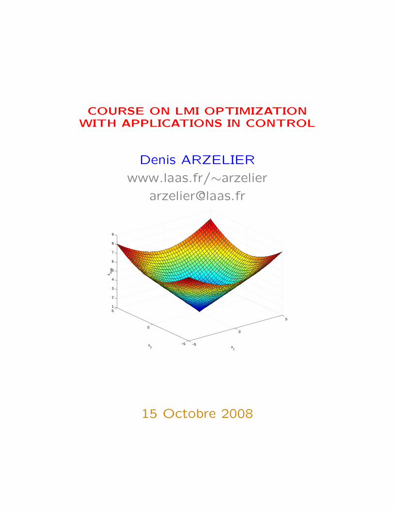
COURSE ON LMI OPTIMIZATIONWITH APPLICATIONS IN CONTROL
Denis ARZELIER
www.laas.fr/∼arzelier
−5
0
5
−5
0
51
2
3
4
5
6
7
8
9
x1
x2
λ max
15 Octobre 2008
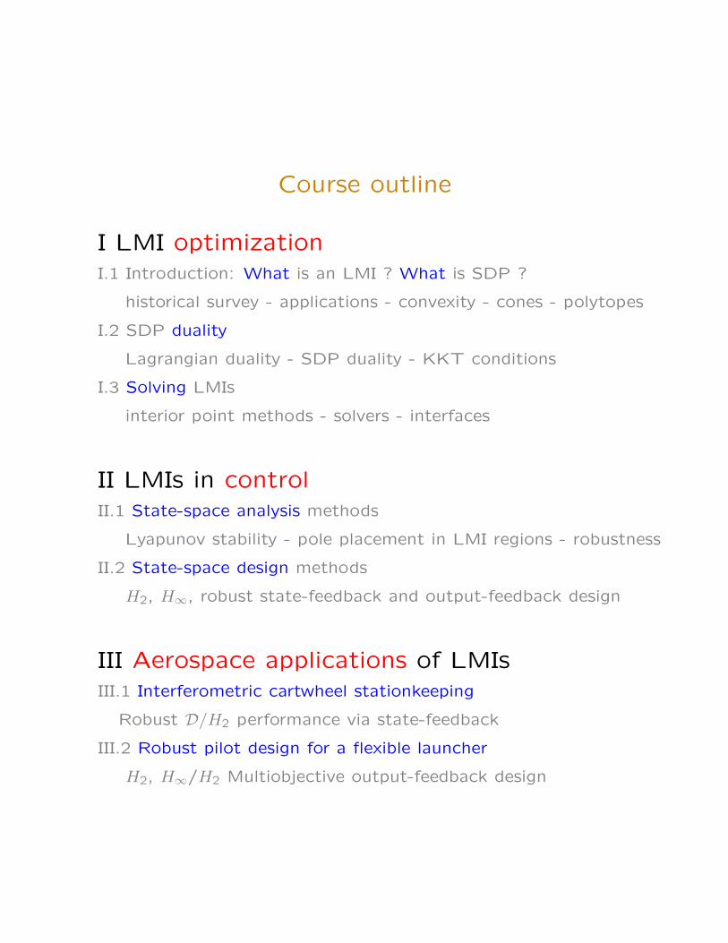
Course outline
I LMI optimizationI.1 Introduction: What is an LMI ? What is SDP ?
historical survey - applications - convexity - cones - polytopes
I.2 SDP duality
Lagrangian duality - SDP duality - KKT conditions
I.3 Solving LMIs
interior point methods - solvers - interfaces
II LMIs in controlII.1 State-space analysis methods
Lyapunov stability - pole placement in LMI regions - robustness
II.2 State-space design methods
H2, H∞, robust state-feedback and output-feedback design
III Aerospace applications of LMIsIII.1 Interferometric cartwheel stationkeeping
Robust D/H2 performance via state-feedback
III.2 Robust pilot design for a flexible launcher
H2, H∞/H2 Multiobjective output-feedback design
Course material
Very good references on convex optimization:• S. Boyd, L. Vandenberghe. Convex Optimization, Lecture Notes
Stanford & UCLA, CA, 2002
• H. Wolkowicz, R. Saigal, L. Vandenberghe. Handbook of semidef-
inite programming, Kluwer, 2000
• A. Ben-Tal, A. Nemirovskii. Lectures on Modern Convex Opti-
mization, SIAM, 2001
Modern state-space LMI methods in control:• C. Scherer, S. Weiland. Course on LMIs in Control, Lecture
Notes Delft & Eindhoven Univ Tech, NL, 2002
• S. Boyd, L. El Ghaoui, E. Feron, V. Balakrishnan. Linear Matrix
Inequalities in System and Control Theory, SIAM, 1994
• M. C. de Oliveira. Linear Systems Control and LMIs, Lecture
Notes Univ Campinas, BR, 2002.
Results on LMI and algebraic optimization incontrol:• P. A. Parrilo, S. Lall. Mini-Course on SDP Relaxations and Al-
gebraic Optimization in Control. European Control Conference,
Cambridge, UK, 2003
• P. A. Parrilo, S. Lall. Semidefinite Programming Relaxations and
Algebraic Optimization in Control, Workshop presented at the 42nd
IEEE Conference on Decision and Control, Maui HI, USA, 2003
COURSE ON LMI OPTIMIZATIONWITH APPLICATIONS IN CONTROL
PART I.1
WHAT IS AN LMI ?
WHAT IS SDP ?
Denis ARZELIER
www.laas.fr/∼arzelier
Professeur Jan C Willems
15 Octobre 2008
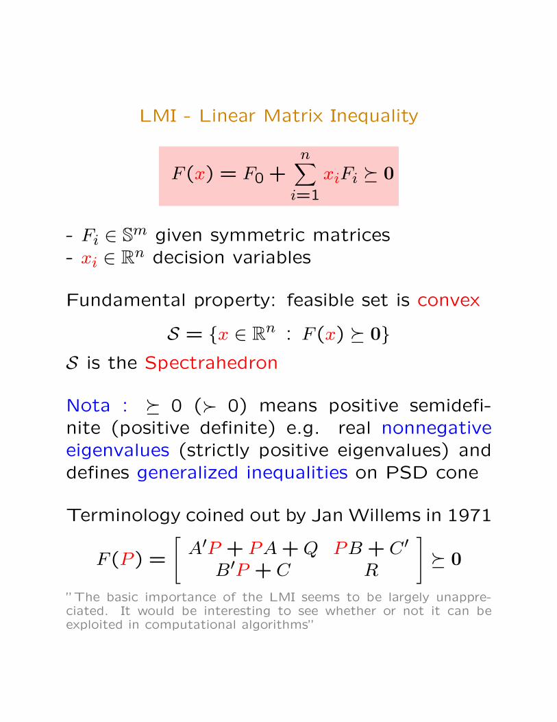
LMI - Linear Matrix Inequality
F (x) = F0 +n∑
i=1
xiFi � 0
- Fi ∈ Sm given symmetric matrices- xi ∈ Rn decision variables
Fundamental property: feasible set is convex
S = {x ∈ Rn : F (x) � 0}S is the Spectrahedron
Nota : � 0 (� 0) means positive semidefi-nite (positive definite) e.g. real nonnegativeeigenvalues (strictly positive eigenvalues) anddefines generalized inequalities on PSD cone
Terminology coined out by Jan Willems in 1971
F (P ) =
[A′P + PA + Q PB + C′
B′P + C R
]� 0
”The basic importance of the LMI seems to be largely unappre-ciated. It would be interesting to see whether or not it can beexploited in computational algorithms”
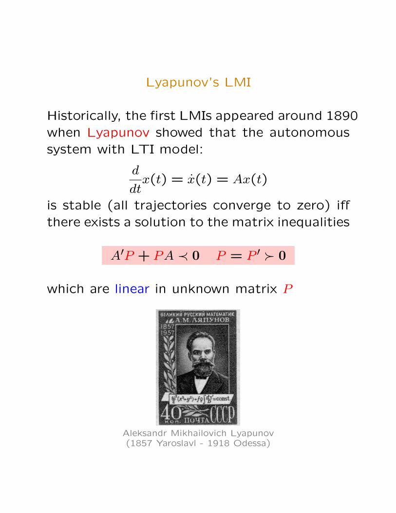
Lyapunov’s LMI
Historically, the first LMIs appeared around 1890when Lyapunov showed that the autonomoussystem with LTI model:
d
dtx(t) = x(t) = Ax(t)
is stable (all trajectories converge to zero) iffthere exists a solution to the matrix inequalities
A′P + PA ≺ 0 P = P ′ � 0
which are linear in unknown matrix P
Aleksandr Mikhailovich Lyapunov(1857 Yaroslavl - 1918 Odessa)
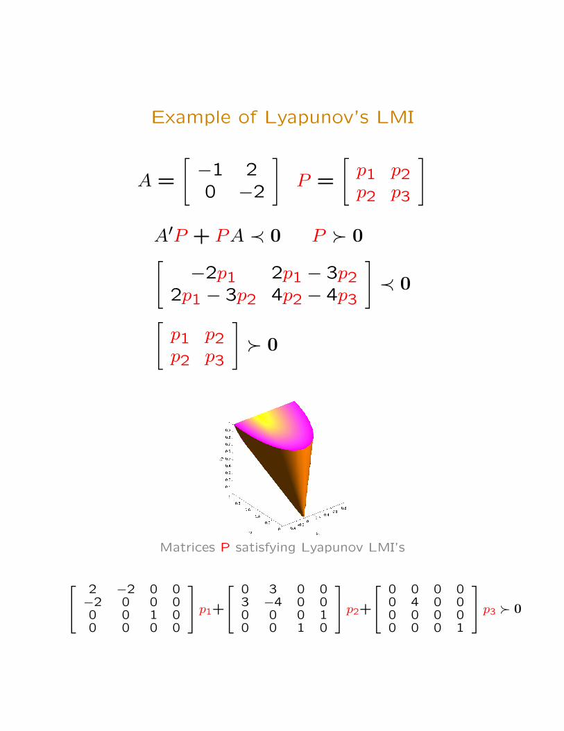
Example of Lyapunov’s LMI
A =
[−1 20 −2
]P =
[p1 p2p2 p3
]
A′P + PA ≺ 0 P � 0[−2p1 2p1 − 3p2
2p1 − 3p2 4p2 − 4p3
]≺ 0
[p1 p2p2 p3
]� 0
Matrices P satisfying Lyapunov LMI’s
[ 2 −2 0 0−2 0 0 00 0 1 00 0 0 0
]p1+
[ 0 3 0 03 −4 0 00 0 0 10 0 1 0
]p2+
[ 0 0 0 00 4 0 00 0 0 00 0 0 1
]p3 � 0
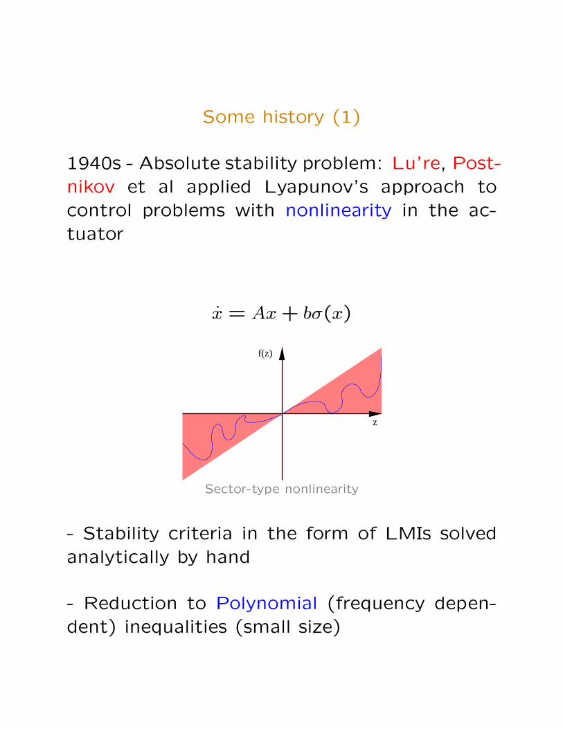
Some history (1)
1940s - Absolute stability problem: Lu’re, Post-nikov et al applied Lyapunov’s approach tocontrol problems with nonlinearity in the ac-tuator
x = Ax + bσ(x)
f(z)
z
Sector-type nonlinearity
- Stability criteria in the form of LMIs solvedanalytically by hand
- Reduction to Polynomial (frequency depen-dent) inequalities (small size)
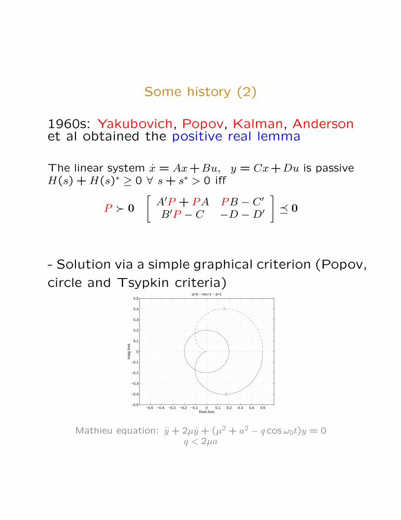
Some history (2)
1960s: Yakubovich, Popov, Kalman, Andersonet al obtained the positive real lemma
The linear system x = Ax+Bu, y = Cx+Du is passiveH(s) + H(s)∗ ≥ 0 ∀ s + s∗ > 0 iff
P � 0
[A′P + PA PB − C ′
B′P − C −D −D′
]� 0
- Solution via a simple graphical criterion (Popov,
circle and Tsypkin criteria)
−0.5 −0.4 −0.3 −0.2 −0.1 0 0.1 0.2 0.3 0.4 0.5−0.5
−0.4
−0.3
−0.2
−0.1
0
0.1
0.2
0.3
0.4
0.5
Real Axis
Imag
Axi
s
q=5 − mu=1 − a=1
Mathieu equation: y + 2µy + (µ2 + a2 − q cosω0t)y = 0q < 2µa
Some history (3)
1971: Willems focused on solving algebraic
Riccati equations (AREs)
A′P + PA− (PB + C′)R−1(B′P + C) + Q = 0
Numerical algebra
H =
[A−BR−1C BR−1B′
−C′R−1C −A′ + C′R−1B′
]V =
V1
V2
Pare = V2V −1
1
By 1971, methods for solving LMIs:
- Direct for small systems
- Graphical methods
- Solving Lyapunov or Riccati equations
Some history (4)
1963: Bellman-Fan: infeasibility criteria formultiple Lyapunov inequalities (duality theory)On Systems of Linear Inequalities in hermitian Matrix Variables
1975: Cullum-Donath-Wolfe: properties of cri-terion and algorithm for minimization of max-imum eigenvaluesThe minimization of certain nondifferentiable sums of eigenvalues
of symmetric matrices
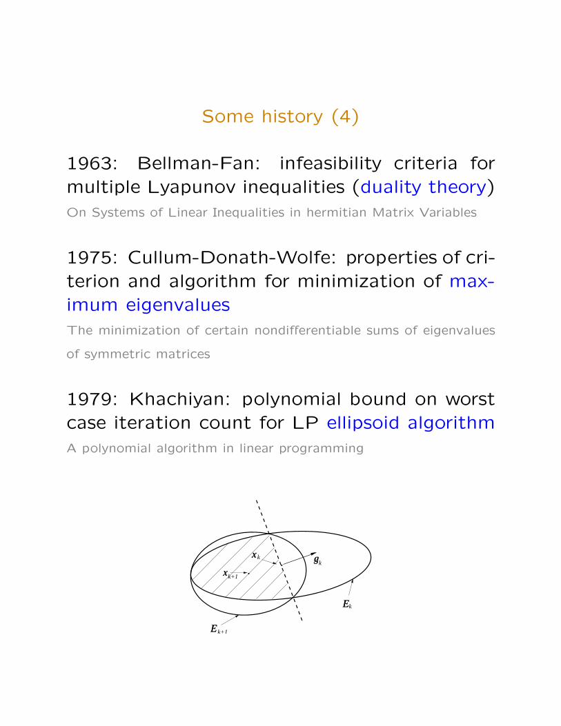
1979: Khachiyan: polynomial bound on worstcase iteration count for LP ellipsoid algorithmA polynomial algorithm in linear programming
E
E
gx
..
x
k
k+1
k+1
kk
Some history (5)
1981: Craven-Mond: Duality theoryLinear Programming with Matrix variables
1984: Karmarkar introduces interior-point (IP)methods for LP: improved complexity boundand efficiency
1985: Fletcher: Optimality conditions for non-differentiable optimizationSemidefinite matrix constraints in optimization
1988: Overton: Nondifferentiable optimiza-tionOn minimizing the maximum eigenvalue of a symmetric matrix
1988: Nesterov, Nemirovski, Alizadeh extendIP methods for convex programmingInterior-Point Polynomial Algorithms in Convex Programming
1990s: most papers on SDP are written (con-trol theory, combinatorial optimization, approx-imation theory...)
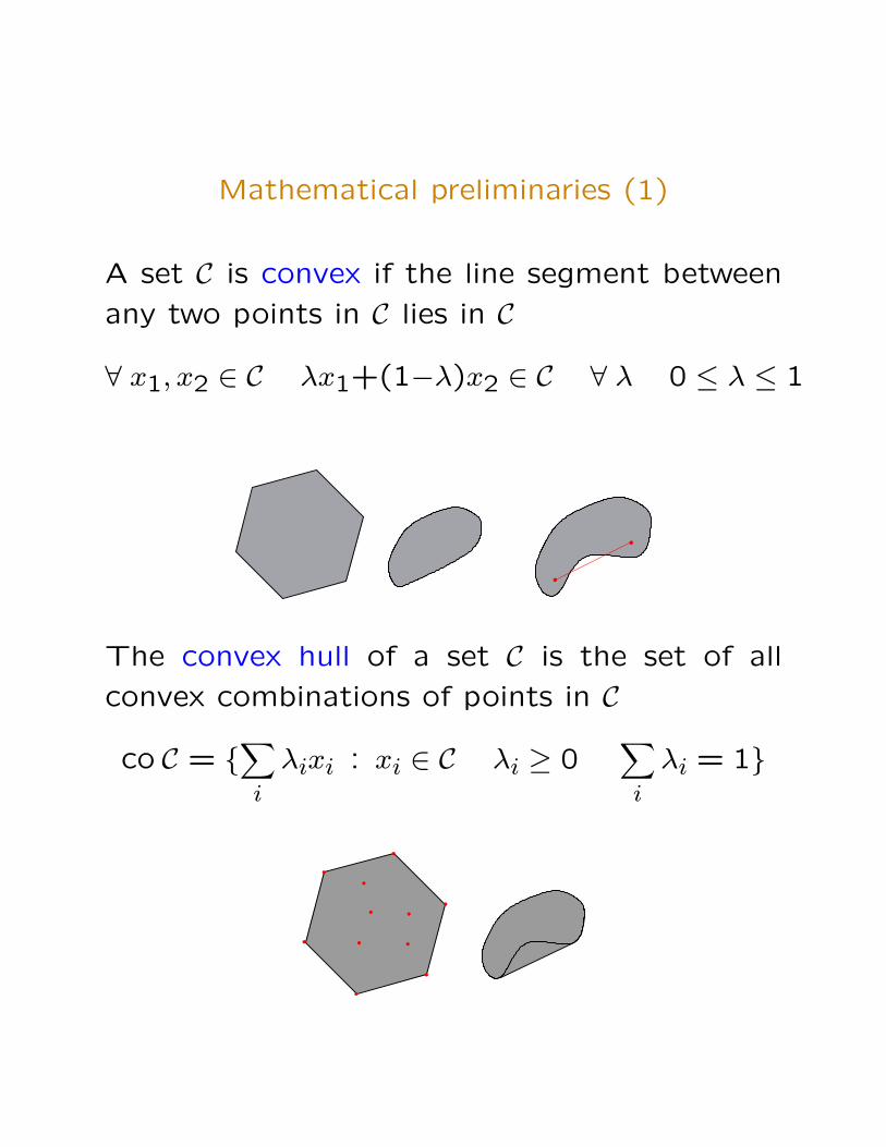
Mathematical preliminaries (1)
A set C is convex if the line segment between
any two points in C lies in C
∀ x1, x2 ∈ C λx1+(1−λ)x2 ∈ C ∀ λ 0 ≤ λ ≤ 1
..
The convex hull of a set C is the set of all
convex combinations of points in C
co C = {∑i
λixi : xi ∈ C λi ≥ 0∑i
λi = 1}
.
.
.
..
.
.
.
.
..
Mathematical preliminaries (2)
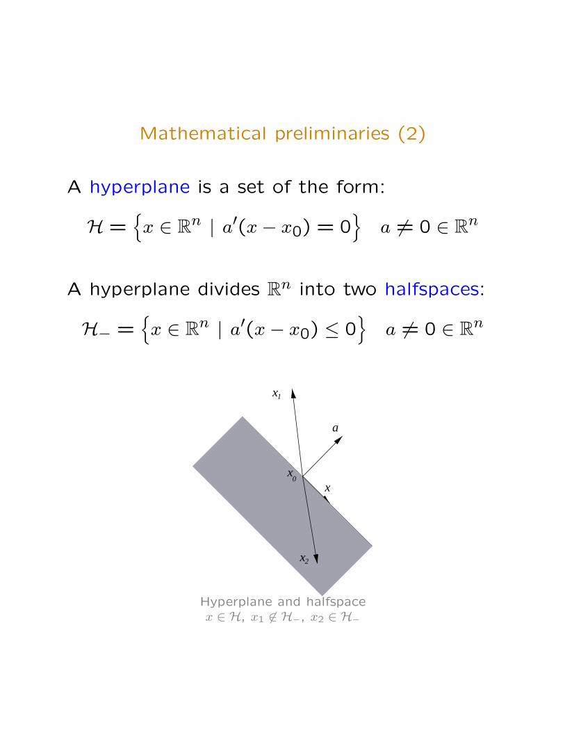
A hyperplane is a set of the form:
H ={x ∈ Rn | a′(x− x0) = 0
}a 6= 0 ∈ Rn
A hyperplane divides Rn into two halfspaces:
H− ={x ∈ Rn | a′(x− x0) ≤ 0
}a 6= 0 ∈ Rn
x
a
x1
0
x2
x
Hyperplane and halfspacex ∈ H, x1 6∈ H−, x2 ∈ H−
Mathematical preliminaries (3)
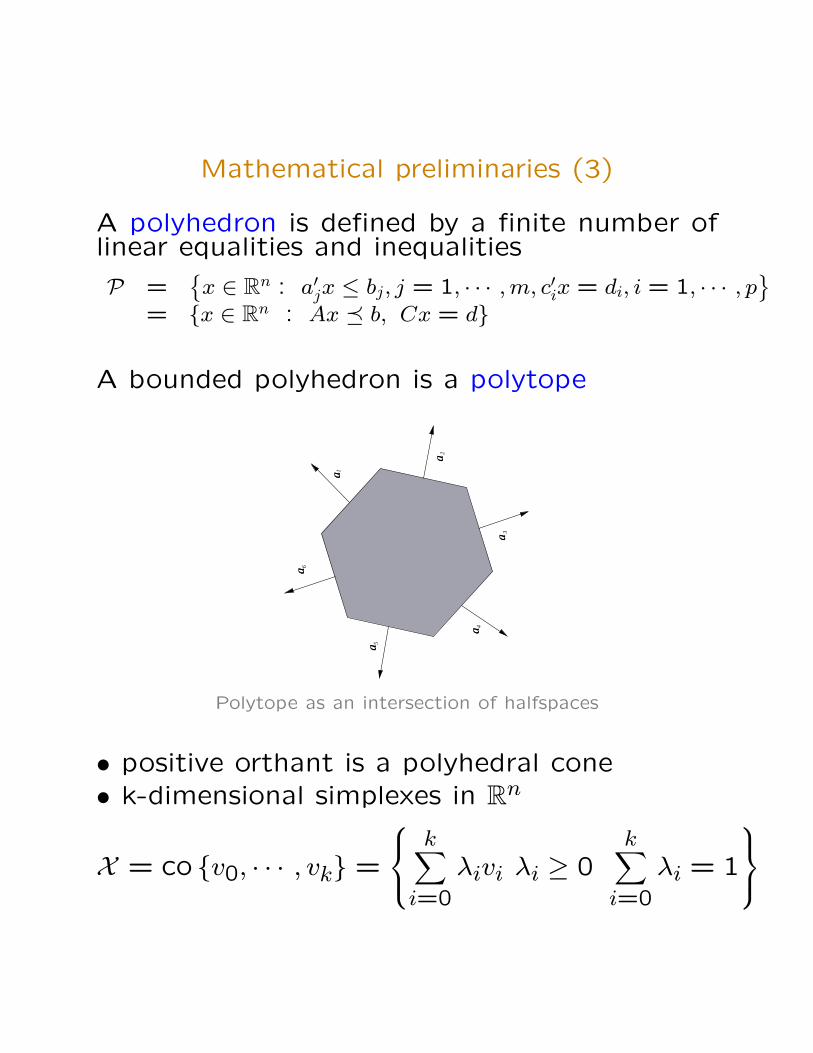
A polyhedron is defined by a finite number oflinear equalities and inequalities
P ={x ∈ Rn : a′jx ≤ bj, j = 1, · · · , m, c′ix = di, i = 1, · · · , p
}= {x ∈ Rn : Ax � b, Cx = d}
A bounded polyhedron is a polytope
a
a
a
a
a
a
1
2
5
6
3
4
Polytope as an intersection of halfspaces
• positive orthant is a polyhedral cone• k-dimensional simplexes in Rn
X = co {v0, · · · , vk} =
k∑
i=0
λivi λi ≥ 0k∑
i=0
λi = 1
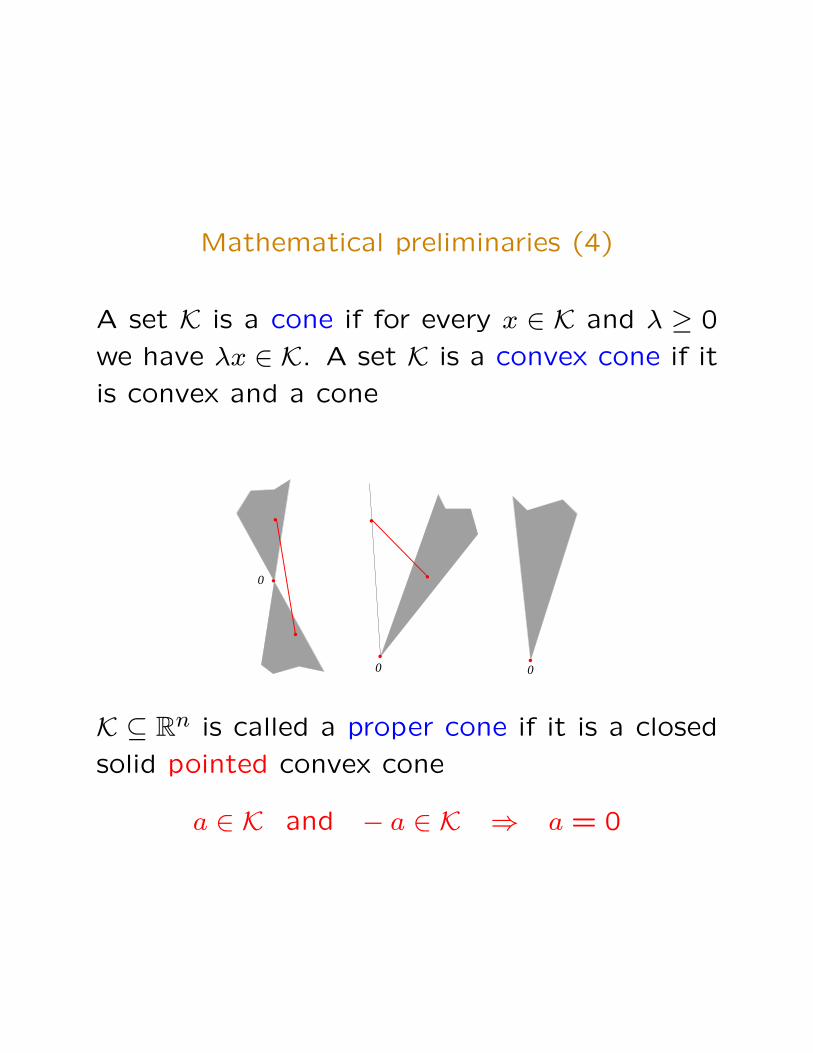
Mathematical preliminaries (4)
A set K is a cone if for every x ∈ K and λ ≥ 0
we have λx ∈ K. A set K is a convex cone if it
is convex and a cone
.
.0
.
.
.0
0 .
.
K ⊆ Rn is called a proper cone if it is a closed
solid pointed convex cone
a ∈ K and − a ∈ K ⇒ a = 0
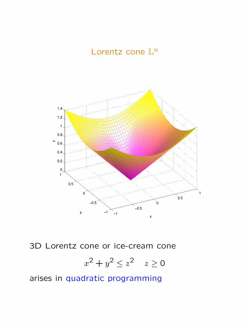
Lorentz cone Ln
3D Lorentz cone or ice-cream cone
x2 + y2 ≤ z2 z ≥ 0
arises in quadratic programming
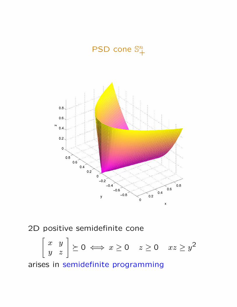
PSD cone Sn+
2D positive semidefinite cone[x yy z
]� 0 ⇐⇒ x ≥ 0 z ≥ 0 xz ≥ y2
arises in semidefinite programming
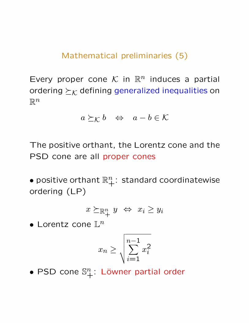
Mathematical preliminaries (5)
Every proper cone K in Rn induces a partial
ordering �K defining generalized inequalities on
Rn
a �K b ⇔ a− b ∈ K
The positive orthant, the Lorentz cone and the
PSD cone are all proper cones
• positive orthant Rn+: standard coordinatewise
ordering (LP)
x �Rn+
y ⇔ xi ≥ yi
• Lorentz cone Ln
xn ≥
√√√√√n−1∑i=1
x2i
• PSD cone Sn+: Lowner partial order
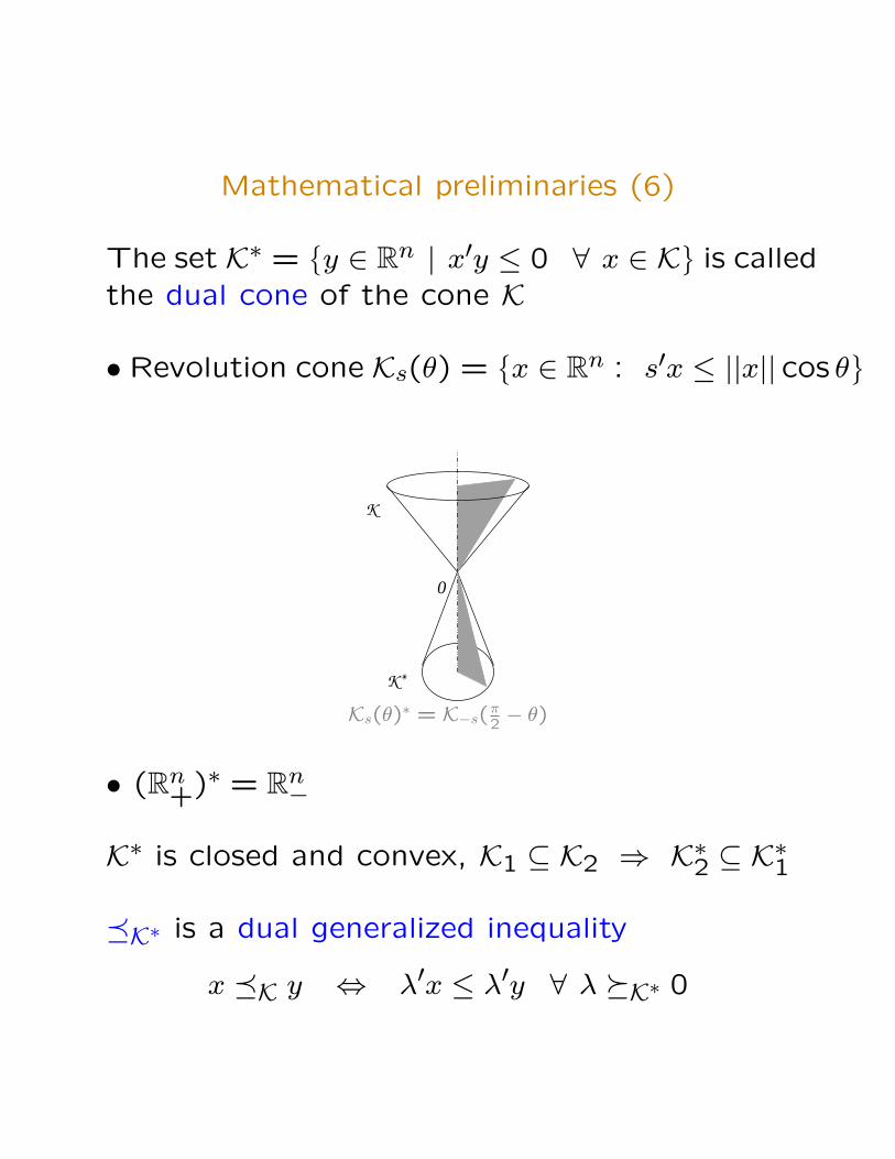
Mathematical preliminaries (6)
The set K∗ ={y ∈ Rn | x′y ≤ 0 ∀ x ∈ K
}is called
the dual cone of the cone K
• Revolution cone Ks(θ) ={x ∈ Rn : s′x ≤ ||x|| cos θ
}
0
Ks(θ)∗ = K−s(π2− θ)
• (Rn+)∗ = Rn
−
K∗ is closed and convex, K1 ⊆ K2 ⇒ K∗2 ⊆ K∗1
�K∗ is a dual generalized inequality
x �K y ⇔ λ′x ≤ λ′y ∀ λ �K∗ 0
Mathematical preliminaries (7)
f : Rn → R is convex if domf is a convex set
and ∀ x, y ∈ domf and 0 ≤ λ ≤ 1
f(λx + (1− λ)y) ≤ λf(x) + (1− λ)f(y)
If f is differentiable: domf is a convex set and
∀ x, y ∈ domf
f(y) ≥ f(x) +∇f(x)′(y − x)
If f is twice differentiable: domf is a convex
set and ∀ x, y ∈ domf
∇2f(x) � 0
Quadratic functions:
f(x) = (1/2)x′Px+q′x+r is convex if and only
if P � 0
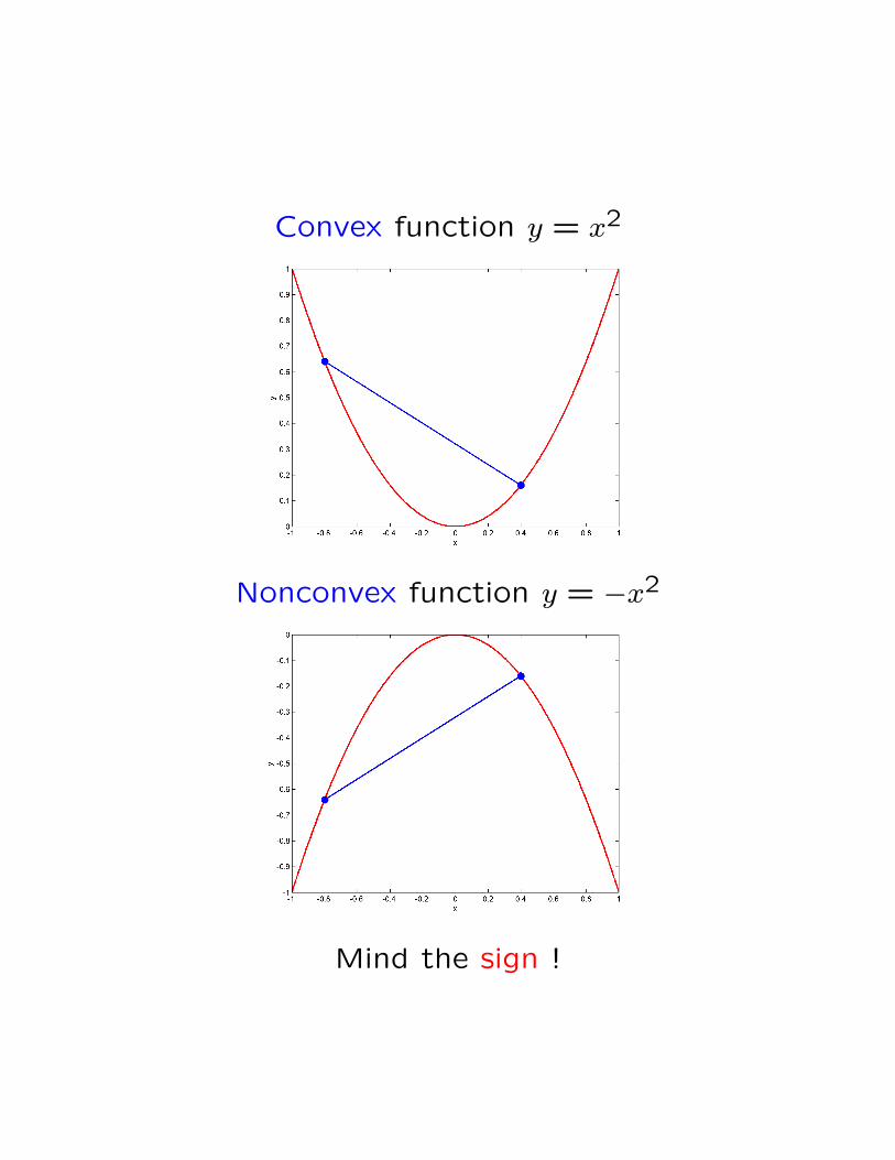
Convex function y = x2
Nonconvex function y = −x2
Mind the sign !
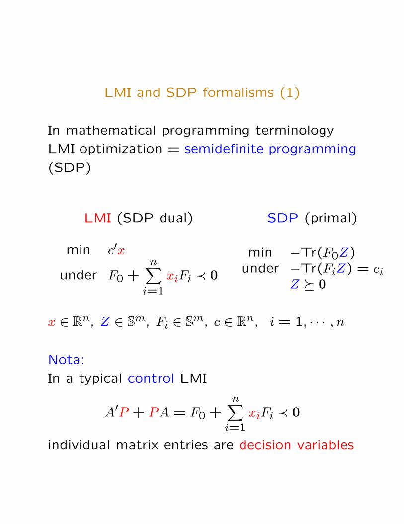
LMI and SDP formalisms (1)
In mathematical programming terminology
LMI optimization = semidefinite programming
(SDP)
LMI (SDP dual) SDP (primal)
min c′x
under F0 +n∑
i=1
xiFi ≺ 0
min −Tr(F0Z)under −Tr(FiZ) = ci
Z � 0
x ∈ Rn, Z ∈ Sm, Fi ∈ Sm, c ∈ Rn, i = 1, · · · , n
Nota:
In a typical control LMI
A′P + PA = F0 +n∑
i=1
xiFi ≺ 0
individual matrix entries are decision variables
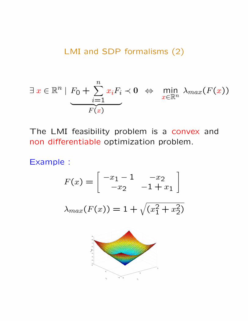
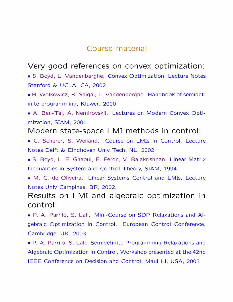
LMI and SDP formalisms (2)
∃ x ∈ Rn | F0 +n∑
i=1
xiFi︸ ︷︷ ︸F (x)
≺ 0 ⇔ minx∈Rn
λmax(F (x))
The LMI feasibility problem is a convex andnon differentiable optimization problem.
Example :
F (x) =
[−x1 − 1 −x2−x2 −1 + x1
]
λmax(F (x)) = 1 +√
(x21 + x2
2)
−5
0
5
−5
0
51
2
3
4
5
6
7
8
9
x1
x2
λ max
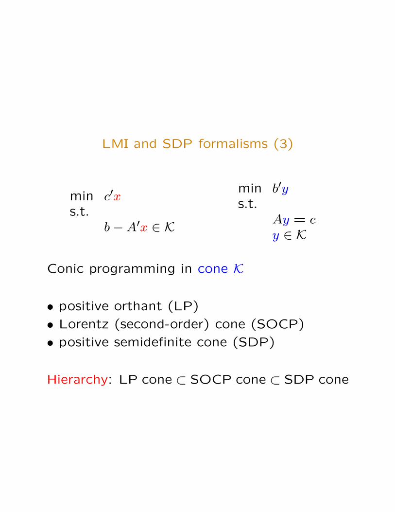
LMI and SDP formalisms (3)
min c′xs.t.
b−A′x ∈ K
min b′ys.t.
Ay = cy ∈ K
Conic programming in cone K
• positive orthant (LP)
• Lorentz (second-order) cone (SOCP)
• positive semidefinite cone (SDP)
Hierarchy: LP cone ⊂ SOCP cone ⊂ SDP cone
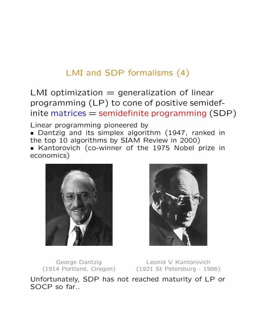
LMI and SDP formalisms (4)
LMI optimization = generalization of linearprogramming (LP) to cone of positive semidef-inite matrices = semidefinite programming (SDP)
Linear programming pioneered by• Dantzig and its simplex algorithm (1947, ranked inthe top 10 algorithms by SIAM Review in 2000)• Kantorovich (co-winner of the 1975 Nobel prize ineconomics)
George Dantzig(1914 Portland, Oregon)
Leonid V Kantorovich(1921 St Petersburg - 1986)
Unfortunately, SDP has not reached maturity of LP orSOCP so far..
Applications of SDP
• control systems (part II of the course)
• robust optimization
• signal processing
• synthesis of antennae arrays
• design of chips
• structural design (trusses)
• geometry (ellipsoids)
• graph theory and combinatorics (MAXCUT,
Shannon capacity)
and many others...
See Helmberg’s page on SDP
www-user.tu-chemnitz.de/∼helmberg/semidef.html
Robust optimization (1)
In many real-life applications of optimizationproblems, exact values of input data (constraints)are seldom known• Uncertainty about the future• Approximations of complexity by uncertainty• Errors in the data• variables may be implemented with errors
min f0(x, u)under fi(x, u) ≤ 0 i = 1, · · · , m
where x ∈ Rn is the vector of decision variablesand u ∈ Rp is the parameters vector.• Stochastic programming• Sensitivity analysis• Interval arithmetic• Worst-case analysis
minx
supu∈U
f0(x, u)
under supu∈U
fi(x, u) ≤ 0 i = 1, · · · , m
Robust optimization (2)
Case study by Ben Tal and Nemirovski:[Math. Programm. 2000]90 LP problems from NETLIB + uncertaintyquite small (just 0.1%) perturbations of ”ob-viously uncertain” data coefficients can makethe ”nominal” optimal solution x∗ heavily in-feasibleRemedy: robust optimization, with robustlyfeasible solutions guaranteed to remain feasi-ble at the expense of possible conservatismRobust conic problem: [Ben Tal Nemirovski96]
minx∈Rn
c′x
s.t. Ax− b ∈ K, ∀ (A, b) ∈ U
This last problem, the so-called robust coun-terpart is still convex, but depending on thestructure of U, can be much harder that origi-nal conic problem
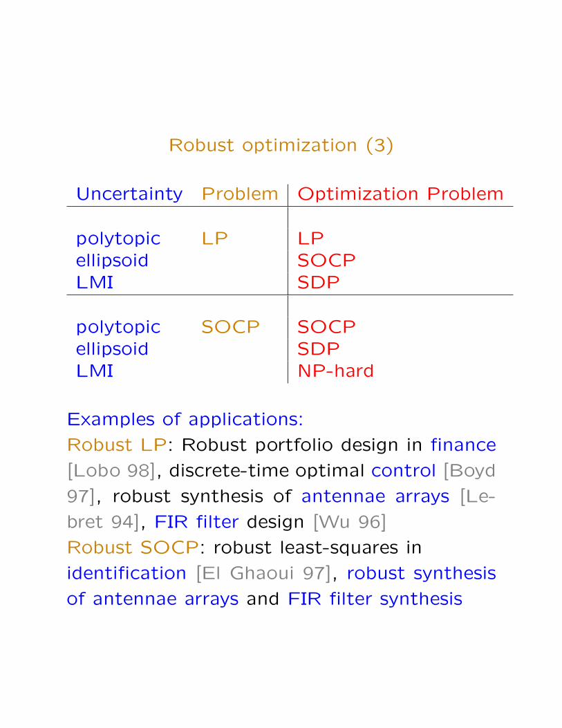
Robust optimization (3)
Uncertainty Problem Optimization Problem
polytopic LP LPellipsoid SOCPLMI SDP
polytopic SOCP SOCPellipsoid SDPLMI NP-hard
Examples of applications:
Robust LP: Robust portfolio design in finance
[Lobo 98], discrete-time optimal control [Boyd
97], robust synthesis of antennae arrays [Le-
bret 94], FIR filter design [Wu 96]
Robust SOCP: robust least-squares in
identification [El Ghaoui 97], robust synthesis
of antennae arrays and FIR filter synthesis
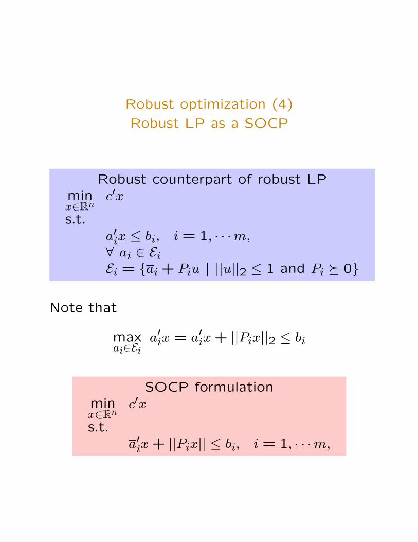
Robust optimization (4)
Robust LP as a SOCP
Robust counterpart of robust LPminx∈Rn
c′x
s.t.a′ix ≤ bi, i = 1, · · ·m,∀ ai ∈ EiEi = {ai + Piu | ||u||2 ≤ 1 and Pi � 0}
Note that
maxai∈Ei
a′ix = a′ix + ||Pix||2 ≤ bi
SOCP formulationminx∈Rn
c′x
s.t.a′ix + ||Pix|| ≤ bi, i = 1, · · ·m,
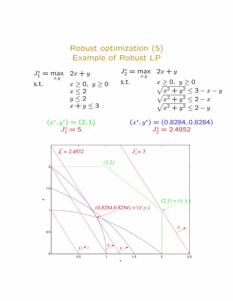
Robust optimization (5)Example of Robust LP
J∗1 = maxx,y
2x + y
s.t. x ≥ 0, y ≥ 0x ≤ 2y ≤ 2x + y ≤ 3
J∗2 = maxx,y
2x + y
s.t. x ≥ 0, y ≥ 0√x2 + y2 ≤ 3− x− y√x2 + y2 ≤ 2− x√x2 + y2 ≤ 2− y
(x∗, y∗) = (2,1) (x∗, y∗) = (0.8284,0.8284)J∗1 = 5 J∗2 = 2.4852
0.5 1 1.5 2 2.50
0.5
1
1.5
2
x
y
*
c
*
*
c
(2,1) = (x ,y )
(1,2)
1
J = 512J = 2.4852 **
c
c
(0.8284,0.8284) = (x ,y )*
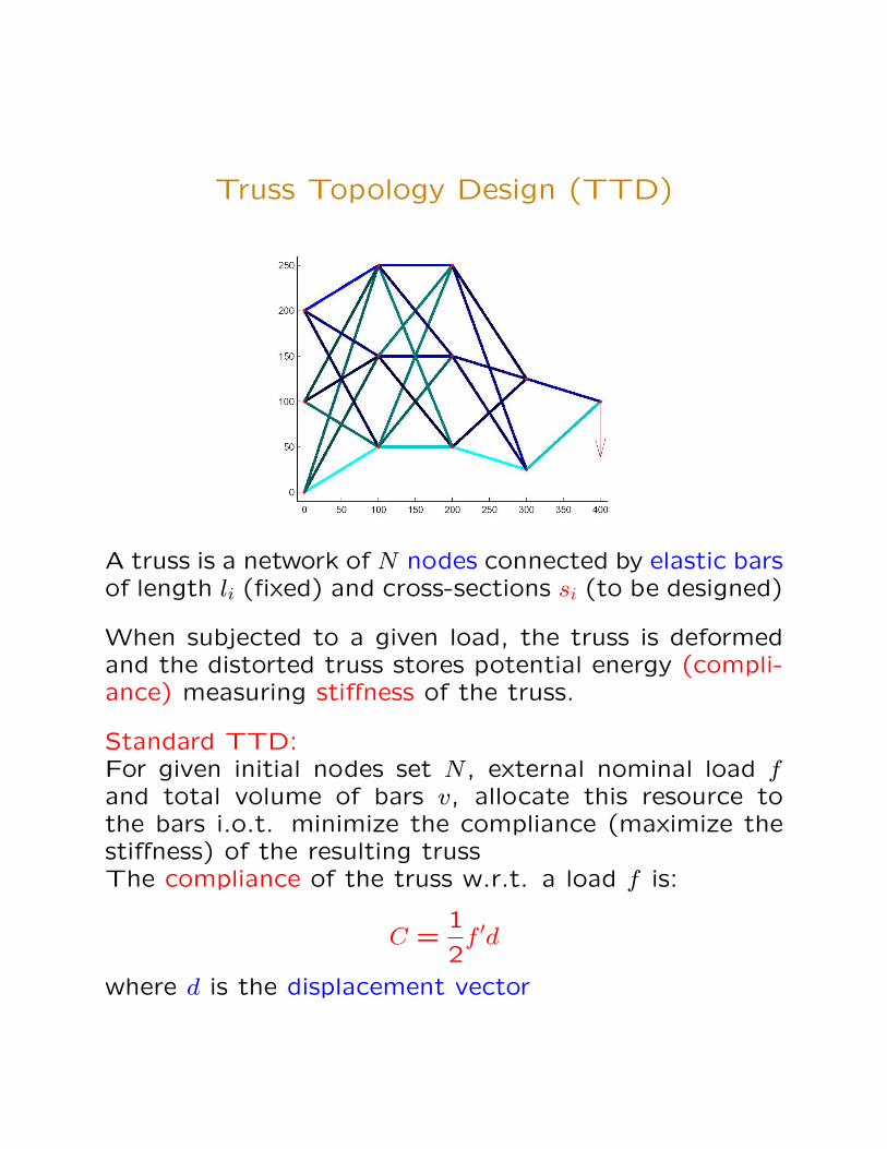
Truss Topology Design (TTD)
A truss is a network of N nodes connected by elastic barsof length li (fixed) and cross-sections si (to be designed)
When subjected to a given load, the truss is deformedand the distorted truss stores potential energy (compli-ance) measuring stiffness of the truss.
Standard TTD:For given initial nodes set N , external nominal load fand total volume of bars v, allocate this resource tothe bars i.o.t. minimize the compliance (maximize thestiffness) of the resulting trussThe compliance of the truss w.r.t. a load f is:
C =1
2f ′d
where d is the displacement vector
Truss Topology Design (2)
Construction reacts to external force f on each
node with displacement vector d satisfying equi-
librium displacement equations:
A(t)d = f
where A(t) is the stiffness matrix, t = l′s is the
volume of the truss.
Linearity assumption: stiffness matrix A(s)
affine in s and positive definite.
A(s) =N∑
i=1
lisibib′i
Constraints on decision variables:
- Bounds on cross-sections:
a ≤ s ≤ b
- Bound on total volume (weight)
l′s =N∑
i=1
lisi ≤ v
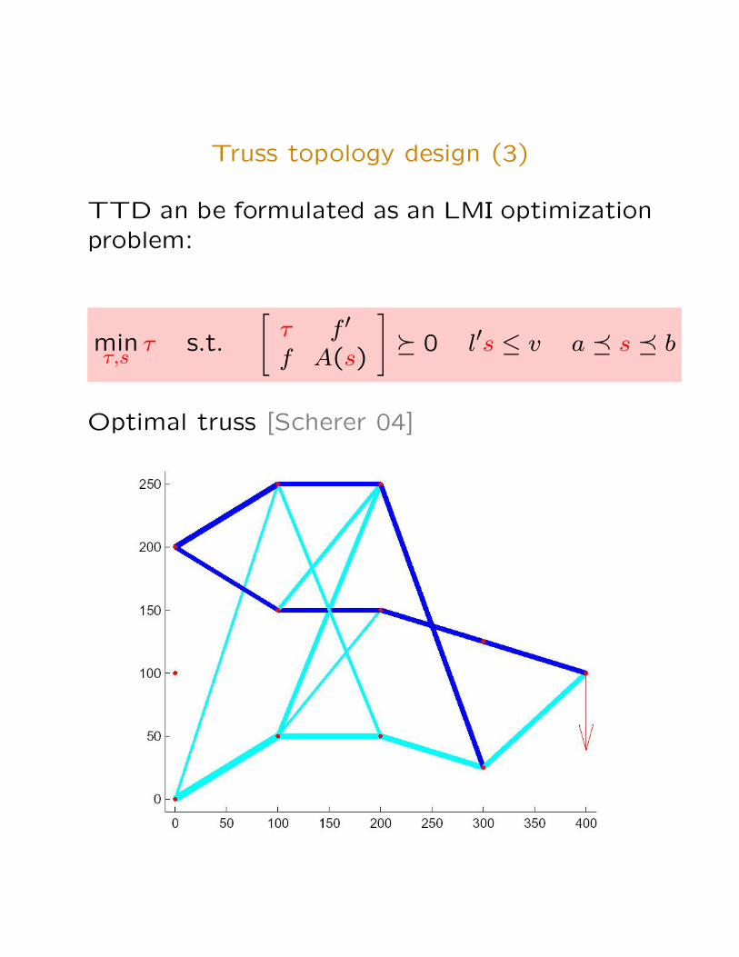
Truss topology design (3)
TTD an be formulated as an LMI optimizationproblem:
minτ,s
τ s.t.
[τ f ′
f A(s)
]� 0 l′s ≤ v a � s � b
Optimal truss [Scherer 04]
Combinatorial optimization (1)
Combinatorics: Graph theory, polyhedral com-
binatorics, combinatorial optimization, enumer-
ative combinatorics...
Definition: Optimization problems in which the
solution space is discrete (finite collection of
objects) or a decision-making problem in which
each decision has a finite (possibly many) num-
ber of feasibilities
Depending upon the formalism
- 0-1 Linear Programming problems: 0-1 Knap-
sack problem,...
- Propositional logic: Maximum satisfiability
problems...
- Constraints satisfaction problems: Airline crew
assignment
- Graph problems: Max-Cut, Shannon capacity
of a graph,...
Combinatorial optimization (2)
- Many CO problems are NP-complete
- Combinatorial explosion (the number of ob-
jects may be huge and grows exponentially in
the size of the representation)
- Scanning all feasibilities (objects) one by one
and choosing the best one is not an option
Two strategies:
- Exact algorithms (not guaranteed to run in
polynomial time)
- Polynomial-time algorithms (guaranteed to
give an optimal solution)
Fundamental concept in CO: Relaxations (com-
binatorial, linear, Lagrangian relaxations)
Optimize over larger easy convex space instead
of optimizing over hard genuine feasible set
- Relaxed solution should be easy to get
- Relaxed solution should be ”close” to the
original
Combinatorial optimization (3)
SDP relaxation of QP in binary variables
(BQP ) maxx∈{−1,1}
x′Qx
Noticing that x′Qx = trace(Qxx′)we get the equivalent form
(BQP ) maxX
trace(QX)
diag(Xii) = e =[1 · · · 1
]′s.t. X � 0
rank(X) = 1
Dropping the non convex rank constraint leads
to the SDP relaxation:
(SDP ) maxX
trace(QX)
s.t. diag(Xii) = e =[1 · · · 1
]′X � 0
Interpretation: lift from Rn to Sn
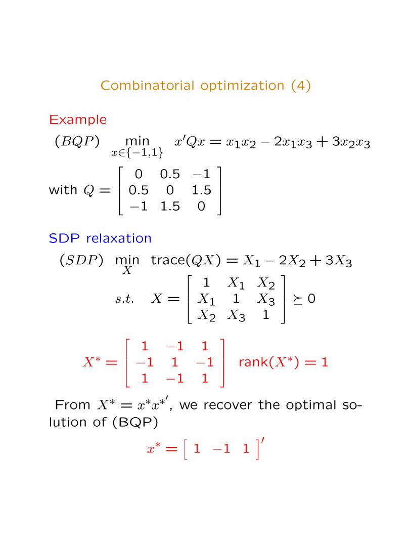
Combinatorial optimization (4)
Example
(BQP ) minx∈{−1,1}
x′Qx = x1x2 − 2x1x3 + 3x2x3
with Q =
0 0.5 −10.5 0 1.5−1 1.5 0
SDP relaxation
(SDP ) minX
trace(QX) = X1 − 2X2 + 3X3
s.t. X =
1 X1 X2X1 1 X3X2 X3 1
� 0
X∗ =
1 −1 1−1 1 −11 −1 1
rank(X∗) = 1
From X∗ = x∗x∗′, we recover the optimal so-
lution of (BQP)
x∗ =[1 −1 1
]′
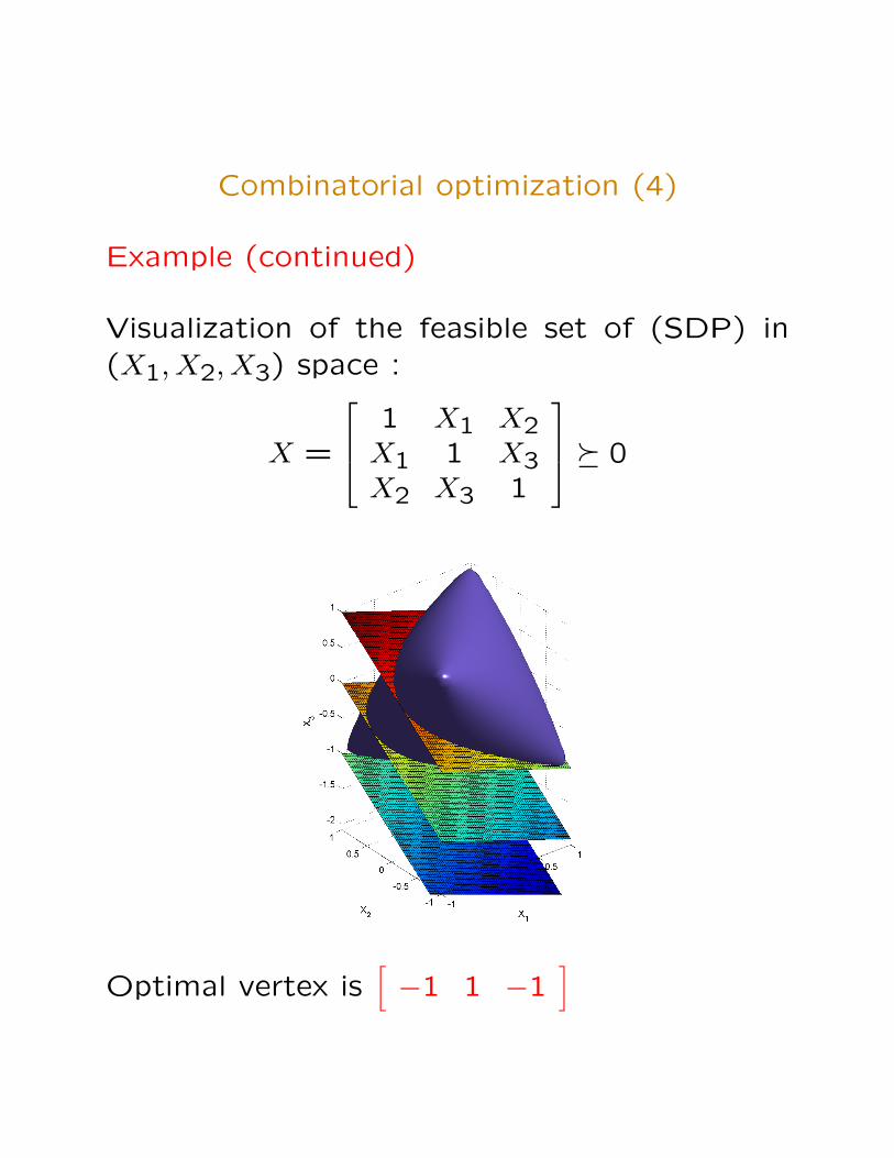
Combinatorial optimization (4)
Example (continued)
Visualization of the feasible set of (SDP) in(X1, X2, X3) space :
X =
1 X1 X2X1 1 X3X2 X3 1
� 0
Optimal vertex is[−1 1 −1
]