Benchmarking with DEA
86
Benchmarking with DEA Introduction to Data Envelopment Analysis September 12 M. Mu˜ noz-M´ arquez [email protected] TeLoYDisRen Research Group http://fqm270.uca.es Statistics and Operation Research Department Cadiz University, Spain
Transcript of Benchmarking with DEA
Benchmarking with DEAIntroduction to Data Envelopment Analysis
September 12
TeLoYDisRen Research Grouphttp://fqm270.uca.es
Statistics and Operation Research DepartmentCadiz University, Spain

Indice
1 Benchmarking with DEA
2 Introduction to DEADEA elementsObjectives and methodology of the DEANotation and formulationExample
3 Selection of variablesThe selection problemSignificance measuresGlobal modelα-ratios or loads
4 Case study
5 Conclusions and future work
6 References
Indice
1 Benchmarking with DEA
2 Introduction to DEADEA elementsObjectives and methodology of the DEANotation and formulationExample
3 Selection of variablesThe selection problemSignificance measuresGlobal modelα-ratios or loads
4 Case study
5 Conclusions and future work
6 References
Indice
1 Benchmarking with DEA
2 Introduction to DEADEA elementsObjectives and methodology of the DEANotation and formulationExample
3 Selection of variablesThe selection problemSignificance measuresGlobal modelα-ratios or loads
4 Case study
5 Conclusions and future work
6 References
Indice
1 Benchmarking with DEA
2 Introduction to DEADEA elementsObjectives and methodology of the DEANotation and formulationExample
3 Selection of variablesThe selection problemSignificance measuresGlobal modelα-ratios or loads
4 Case study
5 Conclusions and future work
6 References
Indice
1 Benchmarking with DEA
2 Introduction to DEADEA elementsObjectives and methodology of the DEANotation and formulationExample
3 Selection of variablesThe selection problemSignificance measuresGlobal modelα-ratios or loads
4 Case study
5 Conclusions and future work
6 References
Indice
1 Benchmarking with DEA
2 Introduction to DEADEA elementsObjectives and methodology of the DEANotation and formulationExample
3 Selection of variablesThe selection problemSignificance measuresGlobal modelα-ratios or loads
4 Case study
5 Conclusions and future work
6 References
Benchmarking with DEAIntroduction to DEASelection of variables
Case studyConclusions and future work
References
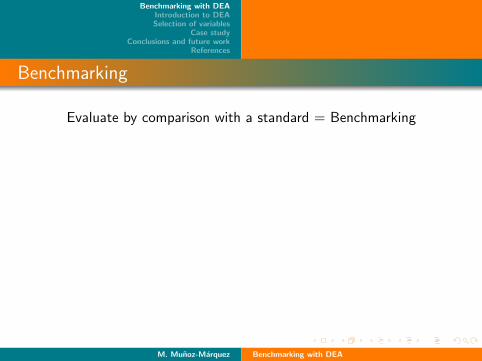
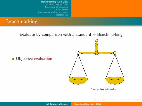
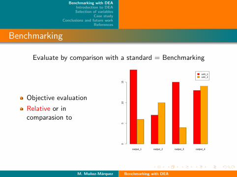
Benchmarking
Evaluate by comparison with a standard = Benchmarking
Objective evaluation
Relative or incomparasion to
Homogeneous results
output_1 output_2 output_3 output_4
unit_1unit_2
05
1015
∗Image from wikimedia
M. Munoz-Marquez Benchmarking with DEA
Benchmarking with DEAIntroduction to DEASelection of variables
Case studyConclusions and future work
References
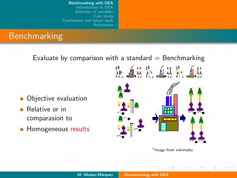
Benchmarking
Evaluate by comparison with a standard = Benchmarking
Objective evaluation
Relative or incomparasion to
Homogeneous results
output_1 output_2 output_3 output_4
unit_1unit_2
05
1015
∗Image from wikimedia
M. Munoz-Marquez Benchmarking with DEA

Benchmarking with DEAIntroduction to DEASelection of variables
Case studyConclusions and future work
References
Motivation
Improvement of the units
Budget distribution
Rewards establishment
Evaluation of the evolution
M. Munoz-Marquez Benchmarking with DEA

Benchmarking with DEAIntroduction to DEASelection of variables
Case studyConclusions and future work
References
Motivation
Improvement of the units
Budget distribution
Rewards establishment
Evaluation of the evolution
M. Munoz-Marquez Benchmarking with DEA

Benchmarking with DEAIntroduction to DEASelection of variables
Case studyConclusions and future work
References
Motivation
Improvement of the units
Budget distribution
Rewards establishment
Evaluation of the evolution
M. Munoz-Marquez Benchmarking with DEA

Benchmarking with DEAIntroduction to DEASelection of variables
Case studyConclusions and future work
References
Motivation
Improvement of the units
Budget distribution
Rewards establishment
Evaluation of the evolution
M. Munoz-Marquez Benchmarking with DEA
Benchmarking with DEAIntroduction to DEASelection of variables
Case studyConclusions and future work
References
Results
Knowledge
Coordination
Attribution
Measures
M. Munoz-Marquez Benchmarking with DEA
Benchmarking with DEAIntroduction to DEASelection of variables
Case studyConclusions and future work
References
Results
Knowledge
Coordination
Attribution
Measures
M. Munoz-Marquez Benchmarking with DEA
Benchmarking with DEAIntroduction to DEASelection of variables
Case studyConclusions and future work
References
Results
Knowledge
Coordination
Attribution
Measures
M. Munoz-Marquez Benchmarking with DEA
Benchmarking with DEAIntroduction to DEASelection of variables
Case studyConclusions and future work
References
Results
Knowledge
Coordination
Attribution
Measures
M. Munoz-Marquez Benchmarking with DEA

Benchmarking with DEAIntroduction to DEASelection of variables
Case studyConclusions and future work
References
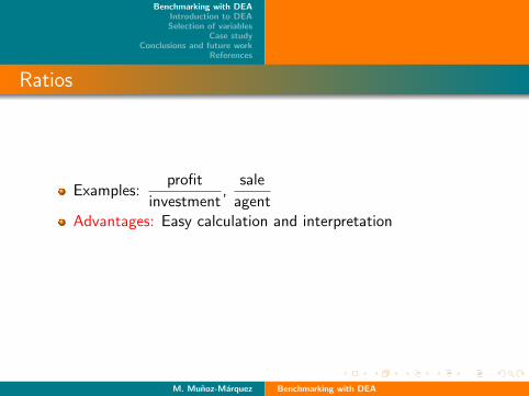
Ratios
Examples:profit
investment,
sale
agent
Advantages: Easy calculation and interpretation
Disadvantages: One-dimensionality, disparity of results,supposes there is no economy of scale
M. Munoz-Marquez Benchmarking with DEA
Benchmarking with DEAIntroduction to DEASelection of variables
Case studyConclusions and future work
References
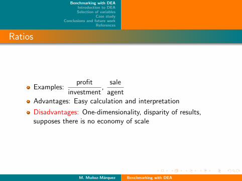
Ratios
Examples:profit
investment,
sale
agentAdvantages: Easy calculation and interpretation
Disadvantages: One-dimensionality, disparity of results,supposes there is no economy of scale
M. Munoz-Marquez Benchmarking with DEA
Benchmarking with DEAIntroduction to DEASelection of variables
Case studyConclusions and future work
References
Frontier models
One prefers: Higher outputs with lower inputs
One does not know: The best way to do that
The way: Estimating the frontier
M. Munoz-Marquez Benchmarking with DEA
Benchmarking with DEAIntroduction to DEASelection of variables
Case studyConclusions and future work
References
Frontier models
One prefers: Higher outputs with lower inputs
One does not know: The best way to do that
The way: Estimating the frontier
M. Munoz-Marquez Benchmarking with DEA
Benchmarking with DEAIntroduction to DEASelection of variables
Case studyConclusions and future work
References
Frontier models
One prefers: Higher outputs with lower inputs
One does not know: The best way to do that
The way: Estimating the frontier
M. Munoz-Marquez Benchmarking with DEA
Benchmarking with DEAIntroduction to DEASelection of variables
Case studyConclusions and future work
References
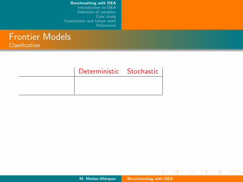
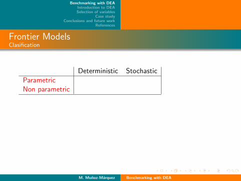
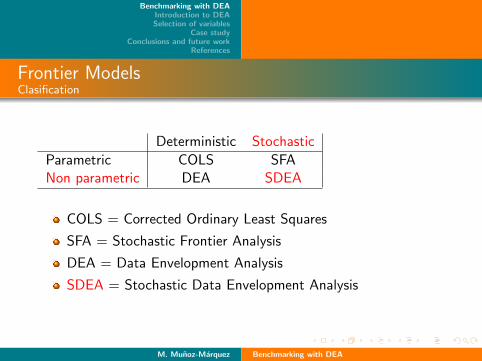
Frontier ModelsClasification
Deterministic Stochastic
Parametric COLS SFANon parametric DEA SDEA
COLS = Corrected Ordinary Least Squares
SFA = Stochastic Frontier Analysis
DEA = Data Envelopment Analysis
SDEA = Stochastic Data Envelopment Analysis
M. Munoz-Marquez Benchmarking with DEA
Benchmarking with DEAIntroduction to DEASelection of variables
Case studyConclusions and future work
References
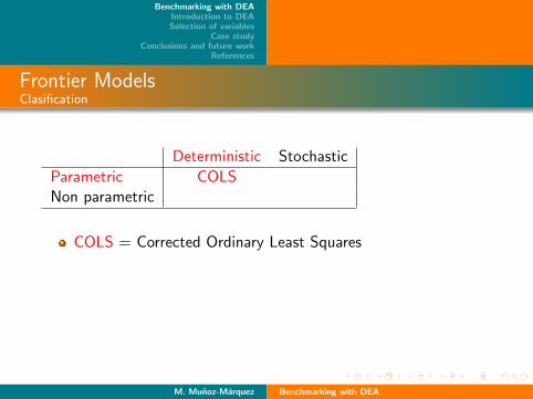
Frontier ModelsClasification
Deterministic Stochastic
Parametric
COLS SFA
Non parametric
DEA SDEA
COLS = Corrected Ordinary Least Squares
SFA = Stochastic Frontier Analysis
DEA = Data Envelopment Analysis
SDEA = Stochastic Data Envelopment Analysis
M. Munoz-Marquez Benchmarking with DEA
Benchmarking with DEAIntroduction to DEASelection of variables
Case studyConclusions and future work
References
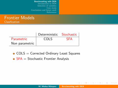
Frontier ModelsClasification
Deterministic Stochastic
Parametric COLS
SFA
Non parametric
DEA SDEA
COLS = Corrected Ordinary Least Squares
SFA = Stochastic Frontier Analysis
DEA = Data Envelopment Analysis
SDEA = Stochastic Data Envelopment Analysis
M. Munoz-Marquez Benchmarking with DEA
Benchmarking with DEAIntroduction to DEASelection of variables
Case studyConclusions and future work
References
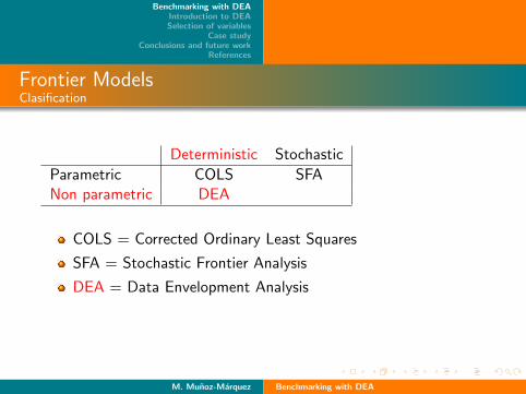
Frontier ModelsClasification
Deterministic Stochastic
Parametric COLS SFANon parametric
DEA SDEA
COLS = Corrected Ordinary Least Squares
SFA = Stochastic Frontier Analysis
DEA = Data Envelopment Analysis
SDEA = Stochastic Data Envelopment Analysis
M. Munoz-Marquez Benchmarking with DEA
Benchmarking with DEAIntroduction to DEASelection of variables
Case studyConclusions and future work
References
Frontier ModelsClasification
Deterministic Stochastic
Parametric COLS SFANon parametric DEA
SDEA
COLS = Corrected Ordinary Least Squares
SFA = Stochastic Frontier Analysis
DEA = Data Envelopment Analysis
SDEA = Stochastic Data Envelopment Analysis
M. Munoz-Marquez Benchmarking with DEA
Benchmarking with DEAIntroduction to DEASelection of variables
Case studyConclusions and future work
References
Frontier ModelsClasification
Deterministic Stochastic
Parametric COLS SFANon parametric DEA SDEA
COLS = Corrected Ordinary Least Squares
SFA = Stochastic Frontier Analysis
DEA = Data Envelopment Analysis
SDEA = Stochastic Data Envelopment Analysis
M. Munoz-Marquez Benchmarking with DEA
Benchmarking with DEAIntroduction to DEASelection of variables
Case studyConclusions and future work
References
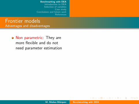
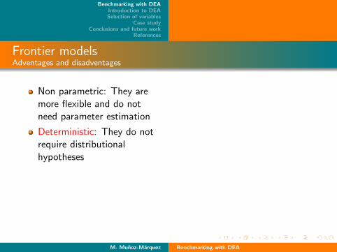
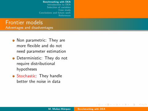
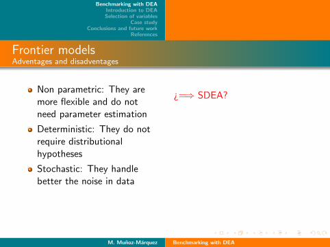
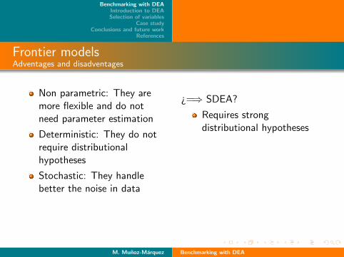
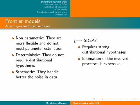
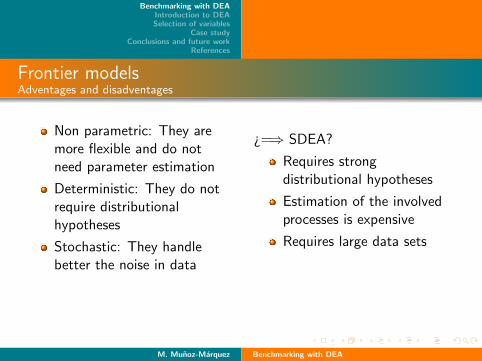
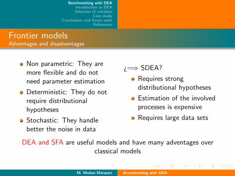
Frontier modelsAdventages and disadventages
Non parametric: They aremore flexible and do notneed parameter estimation
Deterministic: They do notrequire distributionalhypotheses
Stochastic: They handlebetter the noise in data
¿=⇒ SDEA?
Requires strongdistributional hypotheses
Estimation of the involvedprocesses is expensive
Requires large data sets
DEA and SFA are useful models and have many adventages overclassical models
M. Munoz-Marquez Benchmarking with DEA
Benchmarking with DEAIntroduction to DEASelection of variables
Case studyConclusions and future work
References
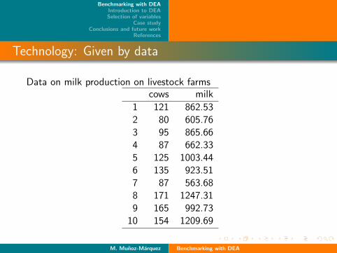
Technology: Given by data
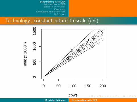
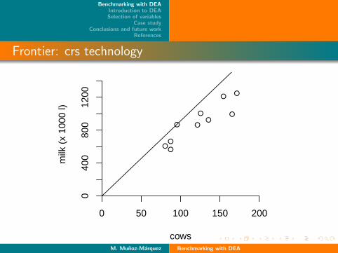
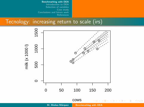
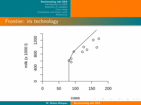
Data on milk production on livestock farmscows milk
1 121 862.532 80 605.763 95 865.664 87 662.335 125 1003.446 135 923.517 87 563.688 171 1247.319 165 992.73
10 154 1209.69
M. Munoz-Marquez Benchmarking with DEA
Benchmarking with DEAIntroduction to DEASelection of variables
Case studyConclusions and future work
References
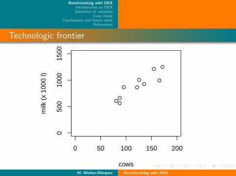
Technologic frontier
●
●
●
●
●●
●
●
●
●
0 50 100 150 200
050
010
0015
00
cows
milk
(x
1000
l)
M. Munoz-Marquez Benchmarking with DEA
Benchmarking with DEAIntroduction to DEASelection of variables
Case studyConclusions and future work
References
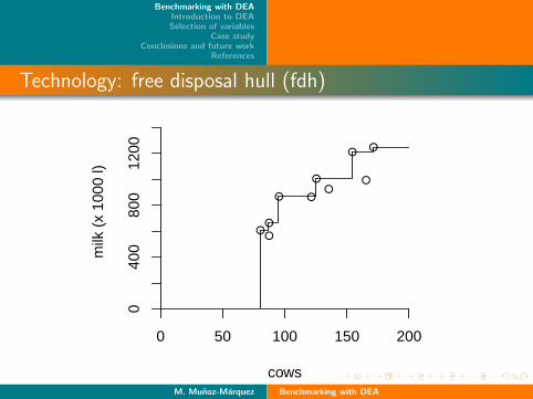
Technology: free disposal hull (fdh)
●
●
●
●
●●
●
●
●
●
0 50 100 150 200
040
080
012
00
cows
milk
(x
1000
l)
M. Munoz-Marquez Benchmarking with DEA
Benchmarking with DEAIntroduction to DEASelection of variables
Case studyConclusions and future work
References
Technology: constant return to scale (crs)
●
●
●
●
●●
●
●
●
●
0 50 100 150 200
050
010
0015
00
cows
milk
(x
1000
l)
M. Munoz-Marquez Benchmarking with DEA
Benchmarking with DEAIntroduction to DEASelection of variables
Case studyConclusions and future work
References
Frontier: crs technology
●
●
●
●
●●
●
●
●
●
0 50 100 150 200
040
080
012
00
cows
milk
(x
1000
l)
M. Munoz-Marquez Benchmarking with DEA
Benchmarking with DEAIntroduction to DEASelection of variables
Case studyConclusions and future work
References
Tecnology: increasing return to scale (irs)
●
●
●
●
●●
●
●
●
●
0 50 100 150 200
050
010
0015
00
cows
milk
(x
1000
l)
M. Munoz-Marquez Benchmarking with DEA
Benchmarking with DEAIntroduction to DEASelection of variables
Case studyConclusions and future work
References
Frontier: irs technology
●
●
●
●
●●
●
●
●
●
0 50 100 150 200
040
080
012
00
cows
milk
(x
1000
l)
M. Munoz-Marquez Benchmarking with DEA
Benchmarking with DEAIntroduction to DEASelection of variables
Case studyConclusions and future work
References
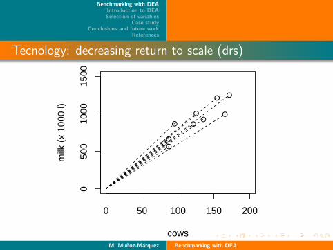
Tecnology: decreasing return to scale (drs)
●
●
●
●
●●
●
●
●
●
0 50 100 150 200
050
010
0015
00
cows
milk
(x
1000
l)
M. Munoz-Marquez Benchmarking with DEA

Benchmarking with DEAIntroduction to DEASelection of variables
Case studyConclusions and future work
References
Frontier: drs tecnology
●
●
●
●
●●
●
●
●
●
0 50 100 150 200
040
080
012
00
cows
milk
(x
1000
l)
M. Munoz-Marquez Benchmarking with DEA
Benchmarking with DEAIntroduction to DEASelection of variables
Case studyConclusions and future work
References
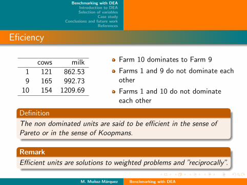
Eficiency
cows milk
1 121 862.539 165 992.73
10 154 1209.69
Farm 10 dominates to Farm 9
Farms 1 and 9 do not dominate eachother
Farms 1 and 10 do not dominateeach other
Definition
The non dominated units are said to be efficient in the sense ofPareto or in the sense of Koopmans.
Remark
Efficient units are solutions to weighted problems and ”reciprocally”.
M. Munoz-Marquez Benchmarking with DEA
Benchmarking with DEAIntroduction to DEASelection of variables
Case studyConclusions and future work
References
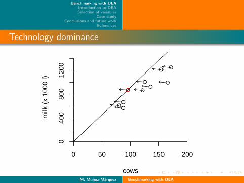
Technology dominance
●
●
●
●
●●
●
●
●
●
0 50 100 150 200
040
080
012
00
cows
milk
(x
1000
l)
●
M. Munoz-Marquez Benchmarking with DEA
Benchmarking with DEAIntroduction to DEASelection of variables
Case studyConclusions and future work
References
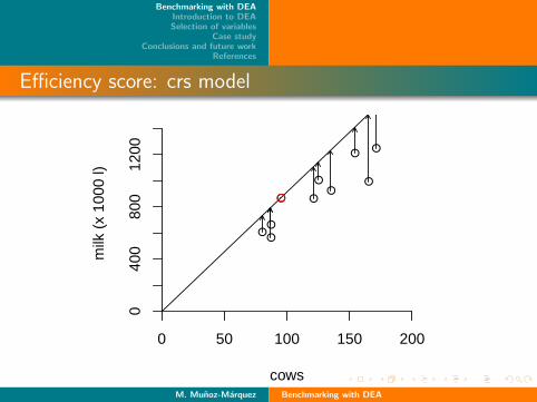
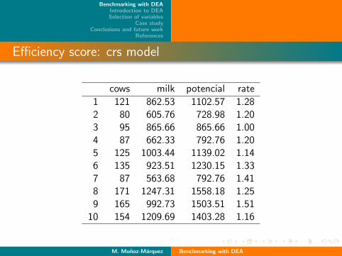
Efficiency score: crs model
●
●
●
●
●●
●
●
●
●
0 50 100 150 200
040
080
012
00
cows
milk
(x
1000
l)
●
M. Munoz-Marquez Benchmarking with DEA
Benchmarking with DEAIntroduction to DEASelection of variables
Case studyConclusions and future work
References
Efficiency score: crs model
cows milk potencial rate
1 121 862.53 1102.57 1.282 80 605.76 728.98 1.203 95 865.66 865.66 1.004 87 662.33 792.76 1.205 125 1003.44 1139.02 1.146 135 923.51 1230.15 1.337 87 563.68 792.76 1.418 171 1247.31 1558.18 1.259 165 992.73 1503.51 1.51
10 154 1209.69 1403.28 1.16
M. Munoz-Marquez Benchmarking with DEA
Benchmarking with DEAIntroduction to DEASelection of variables
Case studyConclusions and future work
References
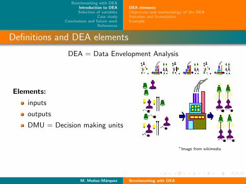
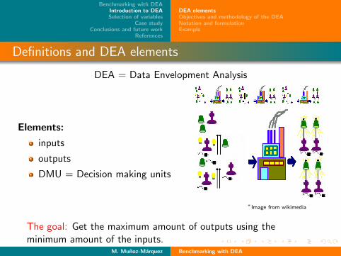
DEA elementsObjectives and methodology of the DEANotation and formulationExample
Definitions and DEA elements
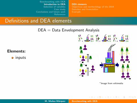
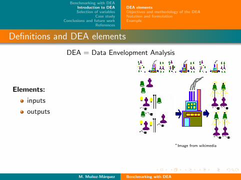
DEA = Data Envelopment Analysis
Elements:
inputs
outputs
DMU = Decision making units
∗Image from wikimedia
The goal: Get the maximum amount of outputs using theminimum amount of the inputs.
M. Munoz-Marquez Benchmarking with DEA
Benchmarking with DEAIntroduction to DEASelection of variables
Case studyConclusions and future work
References
DEA elementsObjectives and methodology of the DEANotation and formulationExample
Definitions and DEA elements
DEA = Data Envelopment Analysis
Elements:
inputs
outputs
DMU = Decision making units
∗Image from wikimedia
The goal: Get the maximum amount of outputs using theminimum amount of the inputs.
M. Munoz-Marquez Benchmarking with DEA
Benchmarking with DEAIntroduction to DEASelection of variables
Case studyConclusions and future work
References
DEA elementsObjectives and methodology of the DEANotation and formulationExample
Objetives of DEA
1 Identify the efficient DMUs
2 Get a rank of DMUs according to their efficiencies
3 Obtain the way that each DMU can be improve
M. Munoz-Marquez Benchmarking with DEA
Benchmarking with DEAIntroduction to DEASelection of variables
Case studyConclusions and future work
References
DEA elementsObjectives and methodology of the DEANotation and formulationExample
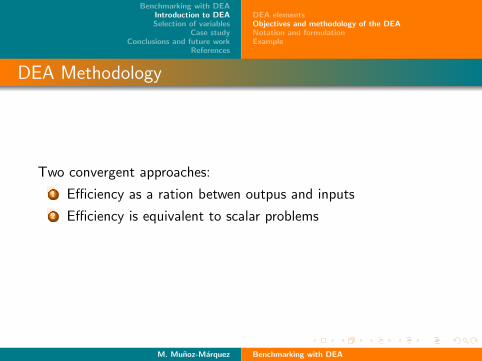
DEA Methodology
Two convergent approaches:
1 Efficiency as a ration betwen outpus and inputs
2 Efficiency is equivalent to scalar problems
Score: Provides a score for each DMU.
M. Munoz-Marquez Benchmarking with DEA
Benchmarking with DEAIntroduction to DEASelection of variables
Case studyConclusions and future work
References
DEA elementsObjectives and methodology of the DEANotation and formulationExample
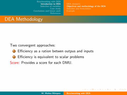
DEA Methodology
Two convergent approaches:
1 Efficiency as a ration betwen outpus and inputs
2 Efficiency is equivalent to scalar problems
Score: Provides a score for each DMU.
M. Munoz-Marquez Benchmarking with DEA
Benchmarking with DEAIntroduction to DEASelection of variables
Case studyConclusions and future work
References
DEA elementsObjectives and methodology of the DEANotation and formulationExample
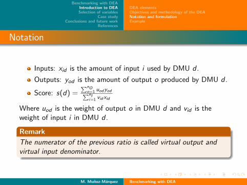
Notation
Inputs: xid is the amount of input i used by DMU d .
Outputs: yod is the amount of output o produced by DMU d .
Score: s(d) =∑nO
o=1 uodyod∑nIi=1 vidxid
Where uod is the weight of output o in DMU d and vid is theweight of input i in DMU d .
Remark
The numerator of the previous ratio is called virtual output andvirtual input denominator.
M. Munoz-Marquez Benchmarking with DEA
Benchmarking with DEAIntroduction to DEASelection of variables
Case studyConclusions and future work
References
DEA elementsObjectives and methodology of the DEANotation and formulationExample
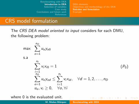
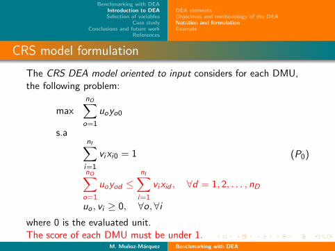
CRS model formulation
The CRS DEA model oriented to input considers for each DMU,the following problem:
max
nO∑o=1
uoyo0
s.anI∑i=1
vixi0 = 1
nO∑o=1
uoyod ≤nI∑i=1
vixid , ∀d = 1, 2, . . . , nD
uo , vi ≥ 0, ∀o,∀i
(P0)
where 0 is the evaluated unit.M. Munoz-Marquez Benchmarking with DEA

Benchmarking with DEAIntroduction to DEASelection of variables
Case studyConclusions and future work
References
DEA elementsObjectives and methodology of the DEANotation and formulationExample
CRS model formulation
The CRS DEA model oriented to input considers for each DMU,the following problem:
max
nO∑o=1
uoyo0
s.anI∑i=1
vixi0 = 1
nO∑o=1
uoyod ≤nI∑i=1
vixid , ∀d = 1, 2, . . . , nD
uo , vi ≥ 0, ∀o,∀i
(P0)
where 0 is the evaluated unit.Fix the amount of input to 1.
M. Munoz-Marquez Benchmarking with DEA
Benchmarking with DEAIntroduction to DEASelection of variables
Case studyConclusions and future work
References
DEA elementsObjectives and methodology of the DEANotation and formulationExample
CRS model formulation
The CRS DEA model oriented to input considers for each DMU,the following problem:
max
nO∑o=1
uoyo0
s.anI∑i=1
vixi0 = 1
nO∑o=1
uoyod ≤nI∑i=1
vixid , ∀d = 1, 2, . . . , nD
uo , vi ≥ 0, ∀o,∀i
(P0)
where 0 is the evaluated unit.The score of each DMU must be under 1.
M. Munoz-Marquez Benchmarking with DEA
Benchmarking with DEAIntroduction to DEASelection of variables
Case studyConclusions and future work
References
DEA elementsObjectives and methodology of the DEANotation and formulationExample
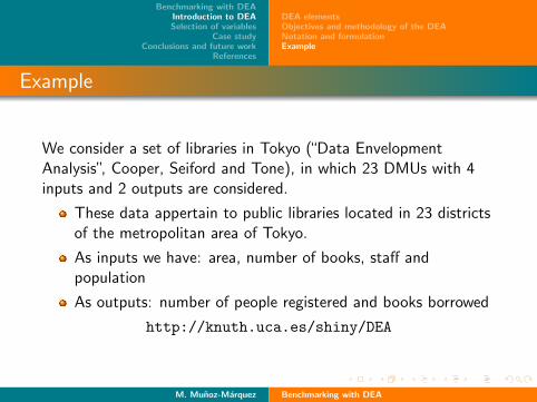
Example
We consider a set of libraries in Tokyo (“Data EnvelopmentAnalysis”, Cooper, Seiford and Tone), in which 23 DMUs with 4inputs and 2 outputs are considered.
These data appertain to public libraries located in 23 districtsof the metropolitan area of Tokyo.
As inputs we have: area, number of books, staff andpopulation
As outputs: number of people registered and books borrowed
http://knuth.uca.es/shiny/DEA
M. Munoz-Marquez Benchmarking with DEA
Benchmarking with DEAIntroduction to DEASelection of variables
Case studyConclusions and future work
References
The selection problemSignificance measuresGlobal modelα-ratios or loads
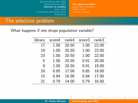
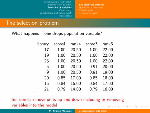
The selection problem
What happens if one drops population variable?
library score4 rank4 score3 rank3
17 1.00 20.50 1.00 22.0019 1.00 20.50 1.00 22.0023 1.00 20.50 1.00 22.00
5 1.00 20.50 0.91 20.009 1.00 20.50 0.91 19.00
20 0.85 17.00 0.85 18.0015 0.84 16.00 0.84 17.0021 0.79 14.00 0.79 16.00
So, one can move units up and down including or removingvariables into the model
M. Munoz-Marquez Benchmarking with DEA
Benchmarking with DEAIntroduction to DEASelection of variables
Case studyConclusions and future work
References
The selection problemSignificance measuresGlobal modelα-ratios or loads
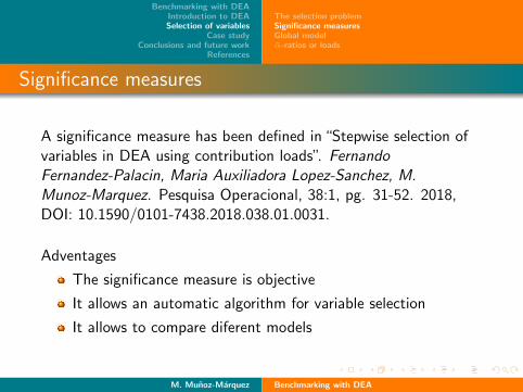
Significance measures
A significance measure has been defined in “Stepwise selection ofvariables in DEA using contribution loads”. FernandoFernandez-Palacin, Maria Auxiliadora Lopez-Sanchez, M.Munoz-Marquez. Pesquisa Operacional, 38:1, pg. 31-52. 2018,DOI: 10.1590/0101-7438.2018.038.01.0031.
Adventages
The significance measure is objective
It allows an automatic algorithm for variable selection
It allows to compare diferent models
M. Munoz-Marquez Benchmarking with DEA
Benchmarking with DEAIntroduction to DEASelection of variables
Case studyConclusions and future work
References
The selection problemSignificance measuresGlobal modelα-ratios or loads
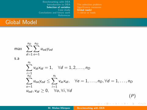
Global Model
max
nD∑d=1
nO∑o=1
uodyod
s.anI∑i=1
vidxid = 1, ∀d = 1, 2, . . . , nD
nO∑o=1
uoeyod ≤nI∑i=1
viexid , ∀e = 1, . . . , nD ,∀d = 1, . . . , nD
uod , vid ≥ 0, ∀o, ∀i ,∀d(P)
M. Munoz-Marquez Benchmarking with DEA
Benchmarking with DEAIntroduction to DEASelection of variables
Case studyConclusions and future work
References
The selection problemSignificance measuresGlobal modelα-ratios or loads
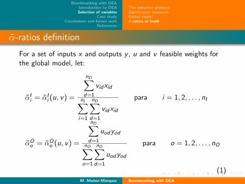
α-ratios definition
For a set of inputs x and outputs y , u and v feasible weights forthe global model, let:
αIi = αI
i (u, v) =
nD∑d=1
vidxid
nI∑i=1
nD∑d=1
vidxid
para i = 1, 2, . . . , nI
αOo = αO
o (u, v) =
nD∑d=1
uodyod
nO∑o=1
nD∑d=1
uodyod
para o = 1, 2, . . . , nO
(1)
M. Munoz-Marquez Benchmarking with DEA
Benchmarking with DEAIntroduction to DEASelection of variables
Case studyConclusions and future work
References
The selection problemSignificance measuresGlobal modelα-ratios or loads
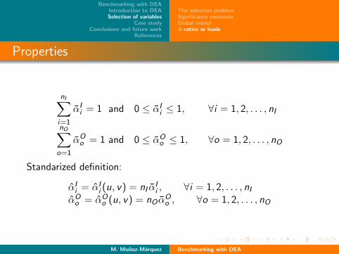
Properties
nI∑i=1
αIi = 1 and 0 ≤ αI
i ≤ 1, ∀i = 1, 2, . . . , nI
nO∑o=1
αOo = 1 and 0 ≤ αO
o ≤ 1, ∀o = 1, 2, . . . , nO
Standarized definition:
αIi = αI
i (u, v) = nI αIi , ∀i = 1, 2, . . . , nI
αOo = αO
o (u, v) = nO αOo , ∀o = 1, 2, . . . , nO
M. Munoz-Marquez Benchmarking with DEA
Benchmarking with DEAIntroduction to DEASelection of variables
Case studyConclusions and future work
References
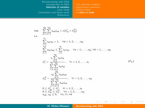
The selection problemSignificance measuresGlobal modelα-ratios or loads
max
nD∑d=1
nO∑o=1
uod yod + ε(αIm + α
Om)
s.anI∑i=1
vid xid = 1, ∀d = 1, 2, . . . , nD
nO∑o=1
uoeyod ≤nI∑i=1
viexid , ∀e = 1, . . . , nD , ∀d = 1, . . . , nD
αIi =
nI
nD∑d=1
vid xid
nI∑i=1
nD∑d=1
vid xid
, ∀i = 1, 2, . . . , nI
αOo =
nO
nD∑d=1
uod yod
nO∑o=1
nD∑d=1
uod yod
, ∀i = 1, 2, . . . , nO
0 ≤ αIm ≤ α
Ii , ∀i = 1, 2, . . . , nI
0 ≤ αOm ≤ α
Oo , ∀o = 1, 2, . . . , nO
uod , vid ≥ 0, ∀o, ∀i, ∀d
(Pα)
M. Munoz-Marquez Benchmarking with DEA
Benchmarking with DEAIntroduction to DEASelection of variables
Case studyConclusions and future work
References
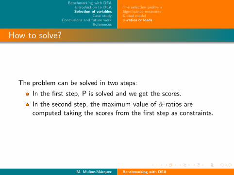
The selection problemSignificance measuresGlobal modelα-ratios or loads
How to solve?
The problem can be solved in two steps:
In the first step, P is solved and we get the scores.
In the second step, the maximum value of α-ratios arecomputed taking the scores from the first step as constraints.
M. Munoz-Marquez Benchmarking with DEA
Benchmarking with DEAIntroduction to DEASelection of variables
Case studyConclusions and future work
References
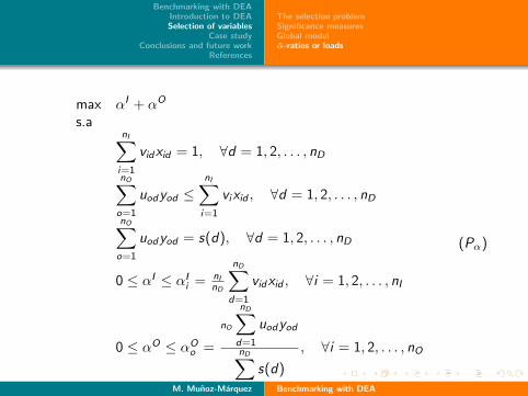
The selection problemSignificance measuresGlobal modelα-ratios or loads
max αI + αO
s.anI∑i=1
vidxid = 1, ∀d = 1, 2, . . . , nD
nO∑o=1
uodyod ≤nI∑i=1
vixid , ∀d = 1, 2, . . . , nD
nO∑o=1
uodyod = s(d), ∀d = 1, 2, . . . , nD
0 ≤ αI ≤ αIi = nI
nD
nD∑d=1
vidxid , ∀i = 1, 2, . . . , nI
0 ≤ αO ≤ αOo =
nO
nD∑d=1
uodyod
nD∑d=1
s(d)
, ∀i = 1, 2, . . . , nO
(Pα)
M. Munoz-Marquez Benchmarking with DEA
Benchmarking with DEAIntroduction to DEASelection of variables
Case studyConclusions and future work
References
The selection problemSignificance measuresGlobal modelα-ratios or loads
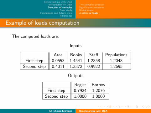
Example of loads computation
The computed loads are:
Inputs
Area Books Staff Populations
First step 0.0553 1.4541 1.2858 1.2048
Second step 0.4011 1.3372 0.9922 1.2695
Outputs
Regist Borrow
First step 0.7924 1.2076
Second step 1.0000 1.0000
M. Munoz-Marquez Benchmarking with DEA
Benchmarking with DEAIntroduction to DEASelection of variables
Case studyConclusions and future work
References
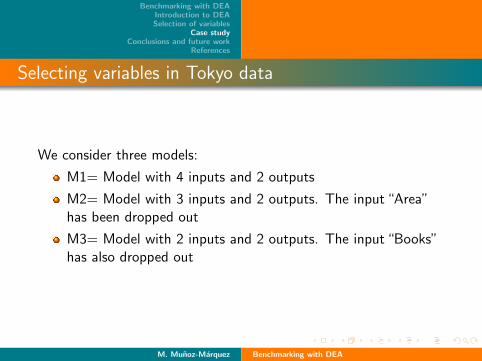
Selecting variables in Tokyo data
We consider three models:
M1= Model with 4 inputs and 2 outputs
M2= Model with 3 inputs and 2 outputs. The input “Area”has been dropped out
M3= Model with 2 inputs and 2 outputs. The input “Books”has also dropped out
M. Munoz-Marquez Benchmarking with DEA

Benchmarking with DEAIntroduction to DEASelection of variables
Case studyConclusions and future work
References
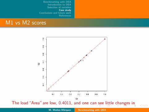
M1 vs M2 scores
The load “Area” are low, 0.4011, and one can see little changes inscores.
M. Munoz-Marquez Benchmarking with DEA
Benchmarking with DEAIntroduction to DEASelection of variables
Case studyConclusions and future work
References
M1 vs M2 scores
The load “Area” are low, 0.4011, and one can see little changes inscores. M. Munoz-Marquez Benchmarking with DEA
Benchmarking with DEAIntroduction to DEASelection of variables
Case studyConclusions and future work
References
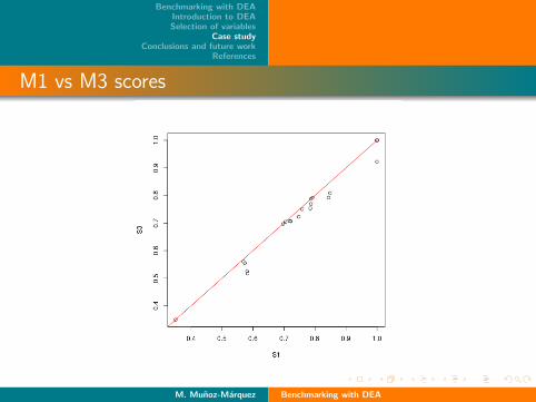
M1 vs M3 scores
The load of “Books” are high, 1.3372, and one can see higherchanges in scores.
M. Munoz-Marquez Benchmarking with DEA

Benchmarking with DEAIntroduction to DEASelection of variables
Case studyConclusions and future work
References
M1 vs M3 scores
The load of “Books” are high, 1.3372, and one can see higherchanges in scores. M. Munoz-Marquez Benchmarking with DEA
Benchmarking with DEAIntroduction to DEASelection of variables
Case studyConclusions and future work
References
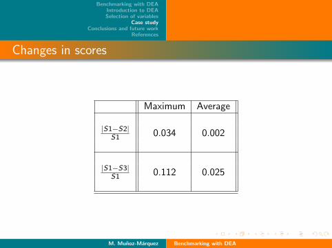
Changes in scores
Maximum Average
|S1−S2|S1 0.034 0.002
|S1−S3|S1 0.112 0.025
M. Munoz-Marquez Benchmarking with DEA
Benchmarking with DEAIntroduction to DEASelection of variables
Case studyConclusions and future work
References
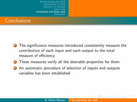
Conclusions
1 The significance measures introduced consistently measure thecontribution of each input and each output to the totalmeasure of efficiency.
2 These measures verify all the desirable properties for them.
3 An automatic procedure of selection of inputs and outputsvariables has been established.
M. Munoz-Marquez Benchmarking with DEA

Benchmarking with DEAIntroduction to DEASelection of variables
Case studyConclusions and future work
References
Future work
1 Continue the development of the software
2 Make a full computational study (in progress)
3 Extend the results to other DEA models
M. Munoz-Marquez Benchmarking with DEA
Benchmarking with DEAIntroduction to DEASelection of variables
Case studyConclusions and future work
References
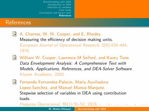
References
A. Charnes, W. W. Cooper, and E. Rhodes.Measuring the efficiency of decision making units.European Journal of Operational Research, 2(6):429–444,1978.
William W. Cooper, Lawrence M Seiford, and Kaoru Tone.Data Envelopment Analysis: A Comprehensive Text withModels, Applications, References, and DEA-Solver Software.Kluwer Academic, 2000.
Fernando Fernandez-Palacin, Marıa AuxiliadoraLopez-Sanchez, and Manuel Munoz-Marquez.Stepwise selection of variables in DEA using contributionloads.Pesquisa Operacional, 38(1):31–52, 2018.
M. Munoz-Marquez Benchmarking with DEA
Benchmarking with DEAIntroduction to Data Envelopment Analysis
September 12
Thank you for your attentionM. Munoz-Marquez
Statistics and Operation Research DepartmentCadiz University, Spain