1

Review of Impulse-Radiating AntennasCarl E. Baum1, Everett G. Farr2, and David V. Giri3

1 Air Force Research Laboratory DEHP3550 Aberdeen Avenue S. E.Kirtland AFB, NM 87117-5776, USATel: 1 (505) 846-5092, Fax: 1 (505) 853-3081

2 Farr Research, Inc.614 Paseo Del Mar N. E.Albuquerque, NM 87123, USATel: 1 (505) 293-3886, Fax: 1 (505) 323-1886e-mail: efarr@farr-research.com

3 Pro-Tech1630 North Main Street, #377Walnut Creek, CA 94596-4609, USATel: 1 (925) 933-0560, Fax: 1 (925) 933-0565e-mail: dgiri@silcon.com

Abstract

This paper reviews the progress to date concerning a special class of antennas knowncollectively as impulse-radiating antennas (IRAs). These are especially suited for radiating veryfast pulses in a narrow beam. A fast-rising step-like signal into the antenna gives an approximatedelta-function response in the far field. The frequency spectrum of the radiated pulse can bevery broad (decades of band ratio). The requisite synthesis of the step-rising plane wave on theantenna aperture can be realized in various ways, including a TEM fed reflector (reflector IRA),TEM (horn) fed lens (lens IRA), and special kinds of arrays (array IRA). Such antennas haveapplication as high-power pulse radiators, transient radars, and antennas capable of operating onmany frequencies simultaneously (due to the large band ratio).

1. Introduction

Of the various types of antennas for radiating and/or receiving transient pulses, we hereare concerned with a special class which are known as impulse-radiating antennas (IRAs).Basically, this type of antenna has the property that, in transmission, a fast-rising (step-like) fieldas a plane wave on the antenna aperture produces an impulse-like far field [2: Baum, 1989].This can be achieved in various ways, the details of which are treated later. For large antennaapertures fed by a single source (pulser) an efficient design uses a conical transmission lineterminated at and feeding a paraboloidal reflector. An alternate design has a conicaltransmission line (TEM horn) feeding a lens with a special resistive termination to the rear of theantenna; for large antennas the lens can be quite massive, but for small antennas this type ofdesign is quite practical. A third approach is a transient array involving many sources feeding anaperture in a manner which purposely has continuity of current from each array element to

2

appropriate adjacent ones so as to achieve efficient radiation, even for wavelengths largecompared to element spacing (but smaller than array linear dimensions) [1: Baum, 1997].

From a historical point of view much of this technology developed out of the nuclearelectromagnetic-pulse (EMP) research, specifically that associated with the large antenna andpulser systems known as EMP simulators used for testing electronic systems [1: Baum, 1978; 1:Smith and Aslin, 1978; 1: Baum, 1992]. The conical transmission waves are a comon feature.Instead of feeding into a cylindrical transmission line or distributed terminator, the conicaltransmission line now feeds a reflector or lens to produce a plane wave at the antenna aperture.However, such lenses have also been considered for use with EMP simulators [7: Baum, 1967].Now, for the IRAs, one is concerned with faster rising pulses, but the antennas are smaller thantypical EMP simulators. So things scale and the basic scientific concepts are, at least in part, thesame.

While the motivation for developing IRA systems has often been to radiate large-amplitude, large-band-ratio (decade or more), undispersed pulses at electronic systems (anddevelop hardening against such environments), it is recognized that such antenna systems havevarious other uses as well. In the remote-sensing arena such antennas are appropriate fortransient radars, including for buried targets (mines and unexploded ordnance (UXO)). Someconsideration has also been given to the possible use for ionospheric research [2: Giri, 1996].Since IRAs have such a large band ratio (ratio of upper to lower useful or roll-off frequencies),they are also being investigated for continuous-wave (CW) application, in which multiplechannels/functions (communications, radar, etc.) use the same antenna [3: Farr et al, 1997].

There is now a large literature on the subject of IRAs; the present paper is intended tosummarize our knowledge of this subject. There are a number of papers which review portionsof this technology and these are grouped together in Section 1 of the Bibliography. With such anextensive literature it is convenient to end this paper with a bibliography which is dividedaccording to subject areas. For reference to papers in this bibliography, the authors are precededby a number, indicating the bibliographic section.

2. Aperture Fields for Impulse -Radiating Antennas

In the normal configuration of an IRA, a focused aperture field is turned on suddenlyover the entire aperture, all at the same time. This idealized step-function time dependence iswell approximated by actual sources that are currently available, although the risetime of a realsource is always non-zero. So if one knows the field radiated by an ideal (step-function) source,one can convolve that result with the derivative of the actual source to obtain the actual field.Thus, we consider here the field radiated by an ideal step-function source. General papersrelating to the radiation from a planar aperture appear in Section 2 of the Bibliography. Thespecial case of a circular aperture is included as Section 9 of the Bibliography.

Consider the aperture shown in Figure 2.1. The field in the aperture is represented by

( )yxE t ′′→

, , with a step-function time dependence that turns on uniformly over the entire aperture.This leads to a radiated field in the far field of [2: Baum, 1989]

3

E r sr

E x y s e dSz t RR

Sa

→ → → → → −= × ′ ′ ×LNM

OQP

′zz( , ) ( , , )12

1 1π

γ γ (2.1)

where γ = s/c, s is the Laplace transform variable, c is the speed of light in free space, and 1→

R isthe vector from the origin of the aperture out to the observation point. This expression simplifiesunder the assumption that we are looking on boresight (in the z- direction). So the radiated fieldon boresight in the far field simplifies to

E r src

ddt

E x y t r c dS t r crc

E x y dx dytS

a tSa a

→ → → →= ′ ′ − ′ = − ′ ′ ′ ′zz zz( , ) ( , , / ) ( / ) ( , )1

2 2πδ

π(2.2)

where the δa(t) function is an approximate Dirac delta function whose area is unity, but whosemagnitude increases proportional to r, and whose width is inversely proportional to r [2:Baum,1989]. So the combination of δa(t)/r has a constant height, even in the limit as r becomes small.A clarification of the shape of the approximate delta function for various aperture fields isprovided in [2: Baum, 1997a]. Other treatments of the exact shape of the delta function arefound in [3: Mikheev, 1997] and [3: Skulkin and Turchin, 1997].

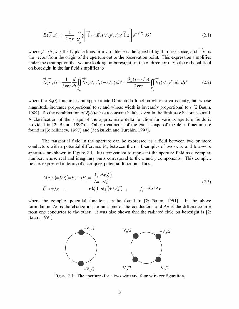
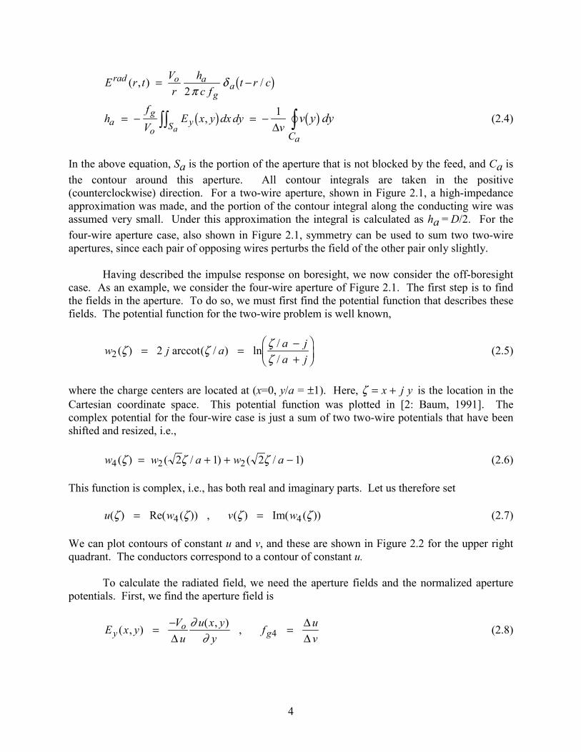
The tangential field in the aperture can be expressed as a field between two or moreconductors with a potential difference Vo between them. Examples of two-wire and four-wireapertures are shown in Figure 2.1. It is convenient to represent the aperture field as a complexnumber, whose real and imaginary parts correspond to the x and y components. This complexfield is expressed in terms of a complex potential function. Thus,

( ) ( ) ( )

( ) ( ) ( ) vufvjuwyjxd

dwu

VEjEEyxE

g

oyx

∆∆=+=+=∆

−=−==

/,,

,

ζζζζζζζ

(2.3)

where the complex potential function can be found in [2: Baum, 1991]. In the aboveformulation, ∆v is the change in v around one of the conductors, and ∆u is the difference in ufrom one conductor to the other. It was also shown that the radiated field on boresight is [2:Baum, 1991]

–Vo/2

+Vo/2

–Vo/2

+Vo/2

–Vo/2

+Vo/2

Figure 2.1. The apertures for a two-wire and four-wire configuration.

4

E r t Vr

hc f

t r crad o a

ga( , ) /= −

2πδ b g

hfV

E x y dx dyva

g

oyS

aa

v y dyC

= − = −zz z,b g b g1∆

(2.4)

In the above equation, Sa is the portion of the aperture that is not blocked by the feed, and Ca isthe contour around this aperture. All contour integrals are taken in the positive(counterclockwise) direction. For a two-wire aperture, shown in Figure 2.1, a high-impedanceapproximation was made, and the portion of the contour integral along the conducting wire wasassumed very small. Under this approximation the integral is calculated as ha = D/2. For thefour-wire aperture case, also shown in Figure 2.1, symmetry can be used to sum two two-wireapertures, since each pair of opposing wires perturbs the field of the other pair only slightly.

Having described the impulse response on boresight, we now consider the off-boresightcase. As an example, we consider the four-wire aperture of Figure 2.1. The first step is to findthe fields in the aperture. To do so, we must first find the potential function that describes thesefields. The potential function for the two-wire problem is well known,

w j a a ja j2 2( ) ( / ) ln /

/ζ ζ ζ

ζ= = −

+FHG

IKJarccot (2.5)

where the charge centers are located at (x=0, y/a = ±1). Here, ζ = +x j y is the location in theCartesian coordinate space. This potential function was plotted in [2: Baum, 1991]. Thecomplex potential for the four-wire case is just a sum of two two-wire potentials that have beenshifted and resized, i.e.,

w w a w a4 2 22 1 2 1( ) ( / ) ( / )ζ ζ ζ= + + − (2.6)

This function is complex, i.e., has both real and imaginary parts. Let us therefore set

u w v w( ) Re( ( )) , ( ) Im( ( ))ζ ζ ζ ζ= =4 4 (2.7)

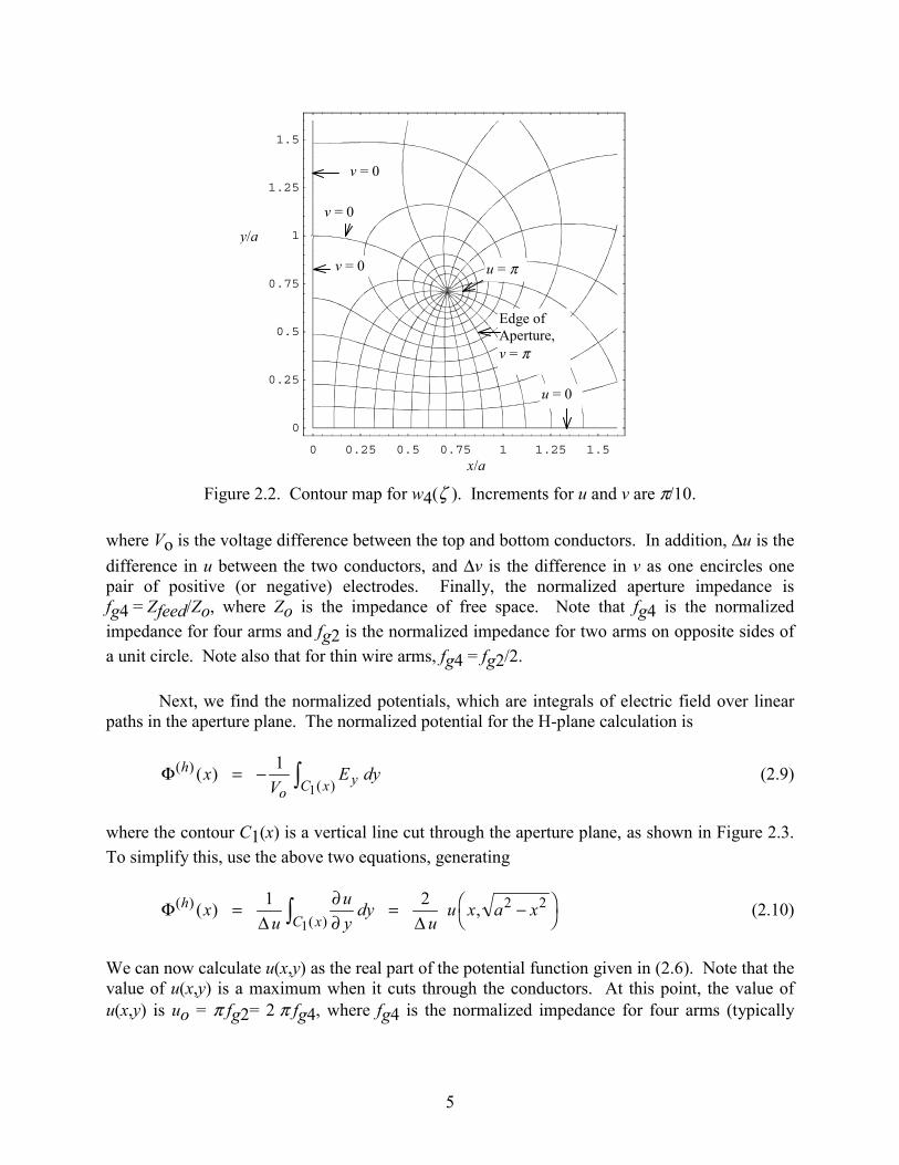
We can plot contours of constant u and v, and these are shown in Figure 2.2 for the upper rightquadrant. The conductors correspond to a contour of constant u.

To calculate the radiated field, we need the aperture fields and the normalized aperturepotentials. First, we find the aperture field is

E x y Vu

u x yy

f uvy

og( , ) ( , ) ,= − =

∆∆∆

∂∂ 4 (2.8)

5

0 0.25 0.5 0.75 1 1.25 1.5

0

0.25

0.5

0.75

1

1.25

1.5

Figure 2.2. Contour map for w4(ζ ). Increments for u and v are π/10.

where Vo is the voltage difference between the top and bottom conductors. In addition, ∆u is thedifference in u between the two conductors, and ∆v is the difference in v as one encircles onepair of positive (or negative) electrodes. Finally, the normalized aperture impedance isfg4 = Zfeed/Zo, where Zo is the impedance of free space. Note that fg4 is the normalizedimpedance for four arms and fg2 is the normalized impedance for two arms on opposite sides ofa unit circle. Note also that for thin wire arms, fg4 = fg2/2.

Next, we find the normalized potentials, which are integrals of electric field over linearpaths in the aperture plane. The normalized potential for the H-plane calculation is

Φ( )( )

( )h

oyC x

xV

E dy= − z11

(2.9)

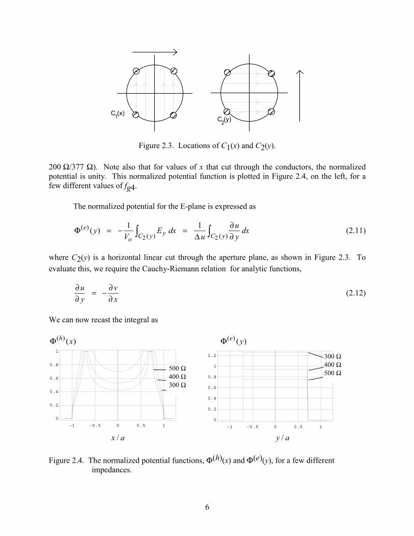
where the contour C1(x) is a vertical line cut through the aperture plane, as shown in Figure 2.3.To simplify this, use the above two equations, generating

Φ∆ ∆

( )( )

( ) ,hC x

xu

uy

dyu

u x a x= ∂∂

= −FH IKz1 21

2 2 (2.10)

We can now calculate u(x,y) as the real part of the potential function given in (2.6). Note that thevalue of u(x,y) is a maximum when it cuts through the conductors. At this point, the value ofu(x,y) is uo = π fg2= 2 π fg4, where fg4 is the normalized impedance for four arms (typically

x/a

y/a

u = π

v = 0

v = 0

u = 0

v = 0

Edge ofAperture,v = π

6

C (x)1

C (y)2

Figure 2.3. Locations of C1(x) and C2(y).

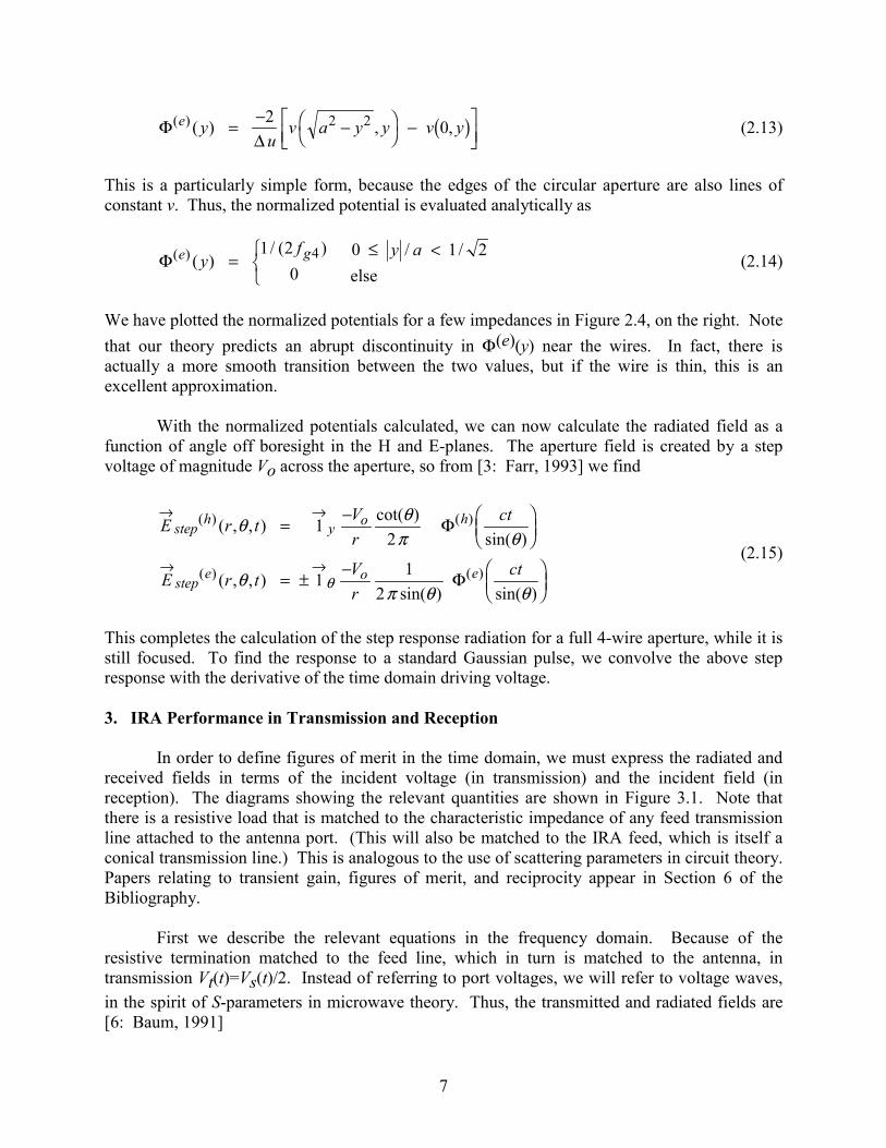
200 Ω/377 Ω). Note also that for values of x that cut through the conductors, the normalizedpotential is unity. This normalized potential function is plotted in Figure 2.4, on the left, for afew different values of fg4.

The normalized potential for the E-plane is expressed as

Φ∆

( )( ) ( )

( )e

oyC y C y

yV

E dxu

uy

dx= − = ∂∂z z1 1

2 2(2.11)

where C2(y) is a horizontal linear cut through the aperture plane, as shown in Figure 2.3. Toevaluate this, we require the Cauchy-Riemann relation for analytic functions,

∂∂

= − ∂∂

uy

vx

(2.12)

We can now recast the integral as

Φ( ) ( )h x Φ( ) ( )e y

-1 -0.5 0 0.5 1

0

0.2

0.4

0.6

0.8

1

-1 -0.5 0 0.5 1

0

0.2

0.4

0.6

0.8

1

1.2

x a/ y a/

Figure 2.4. The normalized potential functions, Φ(h)(x) and Φ(e)(y), for a few differentimpedances.

500 Ω400 Ω300 Ω

300 Ω400 Ω500 Ω

7

Φ∆

( ) ( ) , ,e yu

v a y y v y= − −FH IK −LNM

OQP

2 02 2 b g (2.13)

This is a particularly simple form, because the edges of the circular aperture are also lines ofconstant v. Thus, the normalized potential is evaluated analytically as

Φ( ) ( )/ ( ) / /e gy

f y a=RST

≤ <1 20

0 1 24else

(2.14)

We have plotted the normalized potentials for a few impedances in Figure 2.4, on the right. Notethat our theory predicts an abrupt discontinuity in Φ(e)(y) near the wires. In fact, there isactually a more smooth transition between the two values, but if the wire is thin, this is anexcellent approximation.

With the normalized potentials calculated, we can now calculate the radiated field as afunction of angle off boresight in the H and E-planes. The aperture field is created by a stepvoltage of magnitude Vo across the aperture, so from [3: Farr, 1993] we find

E r t Vr

ct

E r t Vr

ct

steph

y o h

stepe o e

→ →

→ →

= − FHGIKJ

= ± − FHGIKJ

( ) ( )

( ) ( )

( , , ) cot( )sin( )

( , , )sin( ) sin( )

θ θπ θ

θπ θ θθ

12

1 12

Φ

Φ(2.15)

This completes the calculation of the step response radiation for a full 4-wire aperture, while it isstill focused. To find the response to a standard Gaussian pulse, we convolve the above stepresponse with the derivative of the time domain driving voltage.

3. IRA Performance in Transmission and Reception

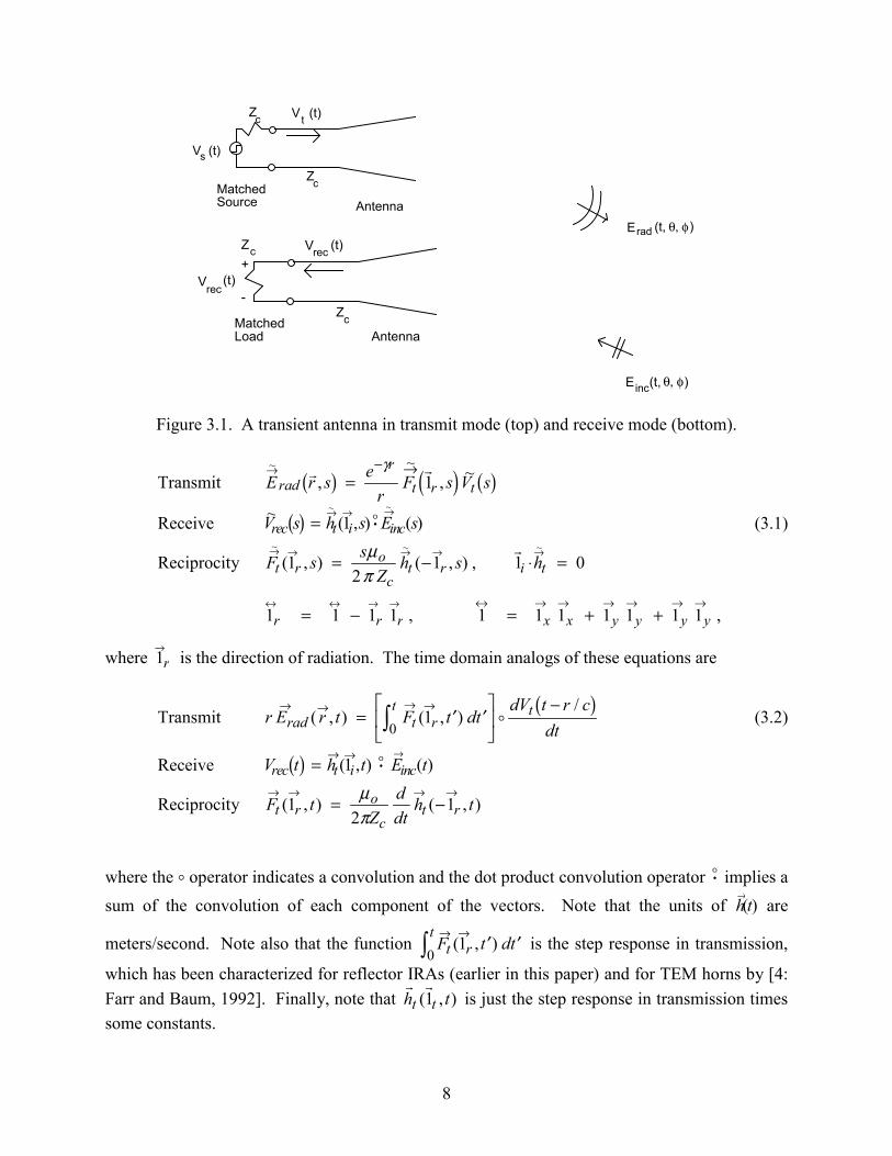
In order to define figures of merit in the time domain, we must express the radiated andreceived fields in terms of the incident voltage (in transmission) and the incident field (inreception). The diagrams showing the relevant quantities are shown in Figure 3.1. Note thatthere is a resistive load that is matched to the characteristic impedance of any feed transmissionline attached to the antenna port. (This will also be matched to the IRA feed, which is itself aconical transmission line.) This is analogous to the use of scattering parameters in circuit theory.Papers relating to transient gain, figures of merit, and reciprocity appear in Section 6 of theBibliography.

First we describe the relevant equations in the frequency domain. Because of theresistive termination matched to the feed line, which in turn is matched to the antenna, intransmission Vt(t)=Vs(t)/2. Instead of referring to port voltages, we will refer to voltage waves,in the spirit of S-parameters in microwave theory. Thus, the transmitted and radiated fields are[6: Baum, 1991]

8

Erad (t, θ, φ

Matched Source Antenna

Vs (t)

Zc

Zc

Vt (t)

)

Matched Load Antenna

+

-Vrec

(t)

Einc(t, θ, φ

Zc

Zc Vrec (t)

)

Figure 3.1. A transient antenna in transmit mode (top) and receive mode (bottom).

Transmit E r s er

F s V sradr

t r t~

, , ~~→=

− →

b g d i b gγ

1

Receive ~ ( , ) ( )~ ~

V s h s E srec t i incb g = → → →⋅1 (3.1)

Reciprocity F s sZ

h s ht ro

ct r i t

~ ~ ~

( , ) ( , ) ,→ → → → →

= − ⋅ =12

1 1 0µπ

1 1 1 1r r r↔ ↔ → →

= − , 1 1 1 1 1 1 1↔ → → → → → →

= + +x x y y y y ,

where 1r→

is the direction of radiation. The time domain analogs of these equations are

Transmit r E r t F t dtdV t r c

dtrad t rt t→ → → →

= ′ ′LNM

OQP

−z( , ) ( , )/

10

b g (3.2)

Receive V t h t E trec t i incb g = → → ⋅ →( , ) ( )1

Reciprocity F tZ

ddt

h tt ro

ct r

→ → → →= −( , ) ( , )1

21µ

π

where the ° operator indicates a convolution and the dot product convolution operator ⋅ implies asum of the convolution of each component of the vectors. Note that the units of h t

→( ) are

meters/second. Note also that the function F t dtt rt → →

′ ′z ( , )10

is the step response in transmission,

which has been characterized for reflector IRAs (earlier in this paper) and for TEM horns by [4:Farr and Baum, 1992]. Finally, note that ),1( th tt

is just the step response in transmission timessome constants.

9

There is a general class of figures of merit for time domain radiators, which we refer to asFM. To find the FM, we drive the antenna with a standard waveshape, such as the integral of aGaussian (in transmission) or a Gaussian (in reception). Because of the above reciprocityrelationship in the time domain we can establish a correlation between the transmit and receivecases. The FM is defined in terms of norms as

Transmission Reception

FMf

V t

E tFM

c f r E t

dV t dtg

rec

inc er

g rad e

incθ φ

θ φθ φ

π θ φ,

, ,, , lim

, ,b g b g

b gb g

b gb g=

⋅=

⋅

→ →

→ →

→∞

1

1

2 1(3.3)

where 1e→

is one of two orthogonal polarizations. The above two definitions are guaranteed to beequal if the driving voltage waveshape in transmission is the integral of the incident electric fieldin reception. One can think of the norm of a function as one of several commonly usedcharacteristics of a time domain function, such as the peak of the function (∞-norm), the integralof magnitude of the function (1-norm), or the square root of “ energy” in the function (2-norm).By way of review, a norm must satisfy three fundamental properties,

f tf t

f t f t f t g t f t g tb g b g b g b g b g b g b g b g=>

≡RST= + ≤ +

00

0 iff otherwise

, ,α α (3.4)

A commonly used norm is the p-norm, which is defined as

( ) ( )tftfdttftft

pp

p sup,)()(/1

≡

≡ ∞

∞

∞− , (3.5)

The choice of the norm will usually be tied to the experimental system. Thus, if a transient radarreceiver responds to the peak magnitude of the received signal, then one should use the ∞-normin the figure of merit definition.

Another useful way of looking at the parameters of an IRA is to consider the relationship

of the impulse response, h t→

θ φ,b g to the standard definitions of gain and effective area. Webegin with the standard expressions in the frequency domain. Thus, the received power is

~ ~ ~( )P A Srec effinc= (3.6)

where ~( )S inc is the incident power density in W/m2 and Aeff is the effective aperture. Gain isrelated to effective aperture by

10

~ ~A Geff = λπ

2

4(3.7)

Combining the above two equations, we have

~~

~( )PG

Srinc=

λπ

2

4(3.8)

Take the square root, and recast into voltages

~ ~ ( )VZ

G EZ

r

c

inc

o=

λπ2

(3.9)

where Zo is the impedance of free space, and Zc, the feed or input impedance, is assumed apositive constant. . Thus, the final result in the frequency domain is

~~

~( )VG f

Erg inc=

λ

π2(3.10)

where fg = Zc/Zo.

Let us now compare the above equation to one that we have been using in the timedomain, where we restrict the consideration to boresight for which symmetry allows us toscalarize the problem as

~ ( ) ( ) ~ ( )( )V t h t E tr tinc= (3.11)

We routinely have already measured ht(t), so we just have to rescale to get gain. Converting thisto the frequency domain, we have

~ ( ) ~ ( ) ~ ( )( )V j h E jr tincω ω ω= (3.12)

Now compare (3.10) and (3.12), to get

~( )| ~ ( ) | | ~ ( ) |

Gh j

ff

ch j

ft

g

t

gω π

λω π ω

= =4 42

2 2

2

2(3.13)

We can use this to scale our ht(t) waveforms to get a frequency-domain gain. Note the similaritybetween (3.7) and (3.13). The implication is that the effective aperture as a function offrequency is |ht(jω)|2/fg , which is a rather simple and pleasing result.

11

There is a drawback with this definition, in that it does not take into account dispersion,or time delay. If different frequencies have different time delays (as happens on moreconventional antennas), the received pulse will not be clean. But the above definition of gaindoes not take this into account. Thus, using this definition of gain, two antennas with the samegain can have very different peak radiated E-fields.

4. Reflector IRA

In Section 2 we described the impulsive portion of the radiation from a focused apertureantenna on boresight. Here, we extend that theory to find a more complete waveform of areflector IRA on boresight. Papers relating to reflector IRAs appear in Section 3 of theBibliography.

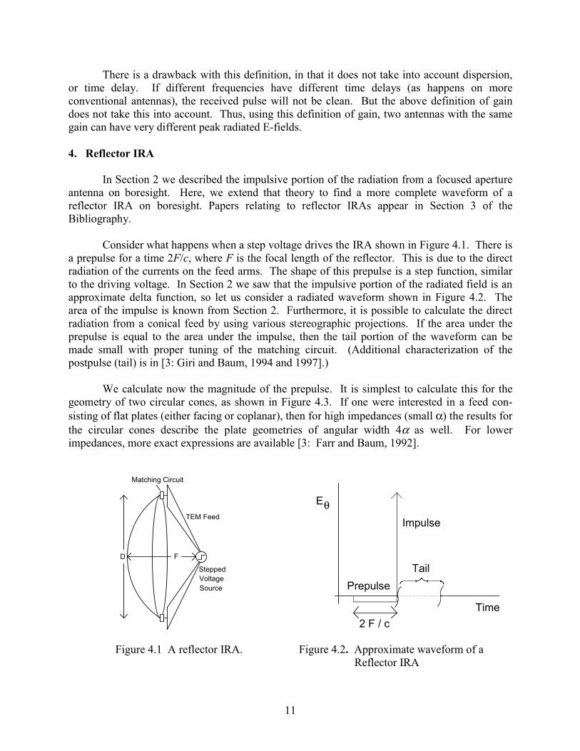
Consider what happens when a step voltage drives the IRA shown in Figure 4.1. There isa prepulse for a time 2F/c, where F is the focal length of the reflector. This is due to the directradiation of the currents on the feed arms. The shape of this prepulse is a step function, similarto the driving voltage. In Section 2 we saw that the impulsive portion of the radiated field is anapproximate delta function, so let us consider a radiated waveform shown in Figure 4.2. Thearea of the impulse is known from Section 2. Furthermore, it is possible to calculate the directradiation from a conical feed by using various stereographic projections. If the area under theprepulse is equal to the area under the impulse, then the tail portion of the waveform can bemade small with proper tuning of the matching circuit. (Additional characterization of thepostpulse (tail) is in [3: Giri and Baum, 1994 and 1997].)

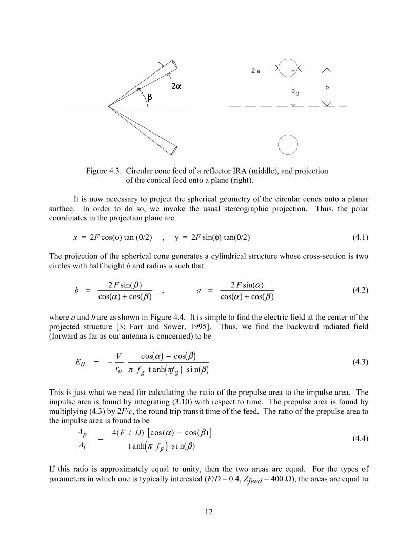
We calculate now the magnitude of the prepulse. It is simplest to calculate this for thegeometry of two circular cones, as shown in Figure 4.3. If one were interested in a feed con-sisting of flat plates (either facing or coplanar), then for high impedances (small α) the results forthe circular cones describe the plate geometries of angular width 4α as well. For lowerimpedances, more exact expressions are available [3: Farr and Baum, 1992].

Matching Circuit

TEM Feed

SteppedVoltageSource

D F

E

Time

Prepulse

Impulse

2 F / c

Tail

θ

Figure 4.1 A reflector IRA. Figure 4.2. Approximate waveform of aReflector IRA

12

ββββ2α 2α 2α 2α

ob b

2 a

Figure 4.3. Circular cone feed of a reflector IRA (middle), and projectionof the conical feed onto a plane (right).

It is now necessary to project the spherical geometry of the circular cones onto a planarsurface. In order to do so, we invoke the usual stereographic projection. Thus, the polarcoordinates in the projection plane are

x = 2F cos(φ) tan (θ/2) , y = 2F sin(φ) tan(θ/2) (4.1)

The projection of the spherical cone generates a cylindrical structure whose cross-section is twocircles with half height b and radius a such that

)cos()cos()sin(2,

)cos()cos()sin(2

βαα

βαβ

+=

+= FaFb (4.2)

where a and b are as shown in Figure 4.4. It is simple to find the electric field at the center of theprojected structure [3: Farr and Sower, 1995]. Thus, we find the backward radiated field(forward as far as our antenna is concerned) to be

E Vr f fo g g

θα β

π π β= −

−cos cos

t anh s i nb g b ge j c h

(4.3)

This is just what we need for calculating the ratio of the prepulse area to the impulse area. Theimpulse area is found by integrating (3.10) with respect to time. The prepulse area is found bymultiplying (4.3) by 2F/c, the round trip transit time of the feed. The ratio of the prepulse area tothe impulse area is found to be

AA

F Df

p

i g=

−4( / ) cos( ) cos( )

t anh s i n( )

α βπ βd i

(4.4)

If this ratio is approximately equal to unity, then the two areas are equal. For the types ofparameters in which one is typically interested (F/D = 0.4, Zfeed = 400 Ω), the areas are equal to

13

better than 1%. Thus, a reasonable expression for the on-boresight radiated field in response to astep-function excitation is

E r tVr

Dcf

cF

u t u t F c t F co

ga( , ) ( ) ( / ) ( / )= − + − + −L

NMOQP4 2

2 2π

δ (4.5)

With a time-varying source, with voltage V(t), the expression is simply

E r t Drcf

cF

V t V t F c dV t F cdtg

( , ) ( ) ( / ) ( / )= − + − + −LNM

OQP4 2

2 2π

(4.6)

Of course, this expression makes use of a number of assumptions, including the use of an idealmatching circuit at the boundary between the feed and reflector. A second assumption is that theaperture blockage is small (valid for thin feed projections). Nevertheless, it is very helpful thatsuch a simple result is available for such a complex structure.

Note that the impulsive portion of the above response was calculated with the assumptionthat the feed is long. This is an unnecessary constraint, as shown by [3: Farr and Baum, 1992].It is shown there that a reflection off a paraboloidal reflector produces a flat phase front with thesame aperture field distribution as an infinitely long cylindrical transmission line (TEM mode),and is exactly expressed by the usual stereographic transformation (with minus sign, reflectortransformation).

Note also that the feed arms in a reflector IRA are normally terminated in thecharacteristic impedance of the feed arms, at a point near the reflector. This serves severalpurposes. First, it drains the high-voltage charge that accumulates on the feed arms. Second, itprovides low-frequency electric and magnetic dipoles that are approximately balanced. Thisleads to a low-frequency pattern of 1+cos(θ), pointing in the correct (boresight) direction.Finally, because the feed is terminated to the reflector in the feed impedance, one can achieve avery good match to the input impedance. Thus, one can get a very flat TDR with this design.

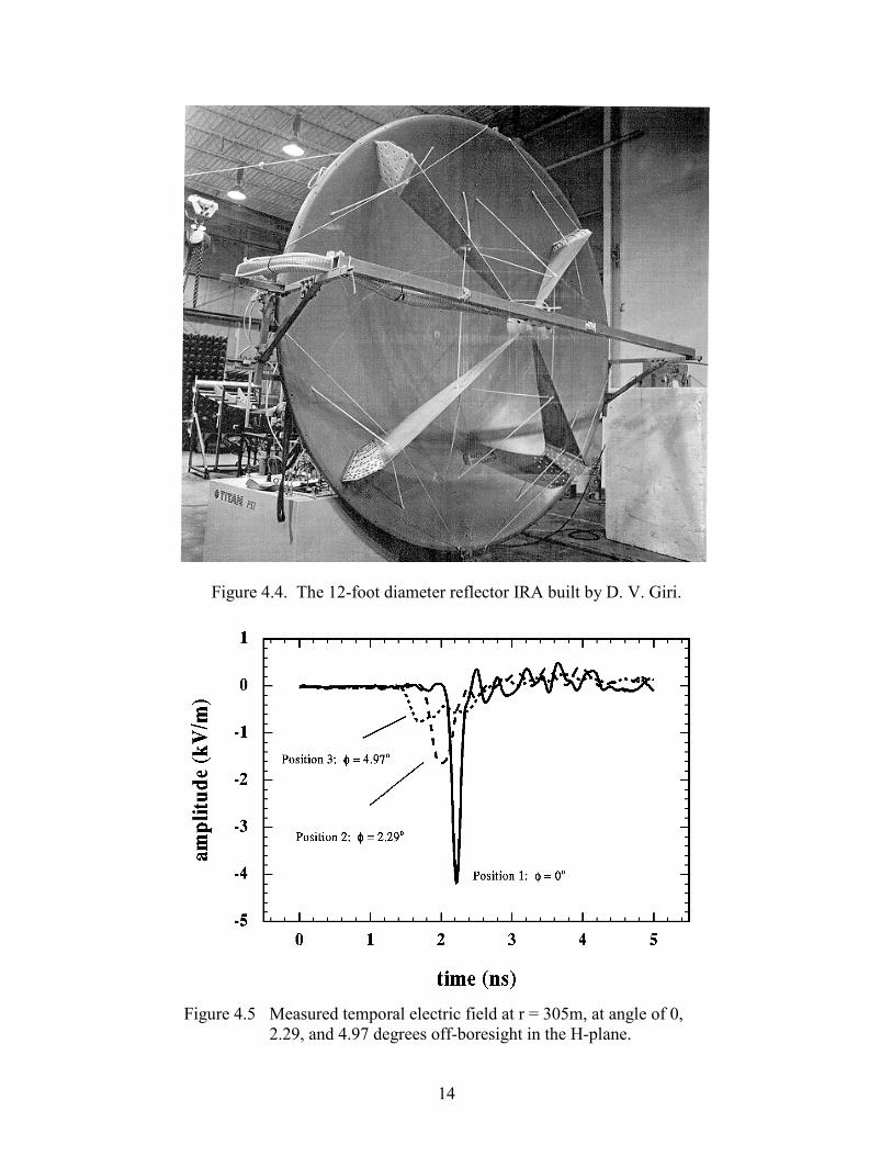
Having described the response of a generic reflector IRA, we now consider a specificexample, which was built by D. V. Giri [3: Giri et al, 1997]. A photograph of the system isshown in Figure 4.4. The system consists of a parabolic reflector illuminated by a pair of conical400 ohm TEM feeds, which are electrically connected near the feed apex. Each of these twin 400ohm feeds incorporate a very low inductance ~100 pF series ceramic capacitors in eachconductor, near the feed apex. The capacitors are then switched by a low inductance, highpressure (~100 atm), hydrogen gas spark gap. The resulting double exponential pulse has a 10-90% risetime of about 100 ps and an e-fold decay of about 20 ns. The system is capable of burstmode operation at up to 200 Hz.

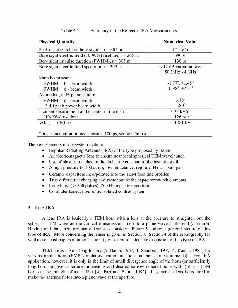
Representative waveforms measured on and near boresight at a distance of 304m isshown in Figure 4.5, [3: Courtney et al, 1995] and other performance parameters are shown inTable 4.1.

14

Figure 4.4. The 12-foot diameter reflector IRA built by D. V. Giri.

Figure 4.5 Measured temporal electric field at r = 305m, at angle of 0,2.29, and 4.97 degrees off-boresight in the H-plane.

15

Table 4.1 Summary of the Reflector IRA Measurements

Physical Quantity Numerical Value

Peak electric field on bore sight at r = 305 m 4.2 kV/mBore sight electric field (10-90%) risetime, r = 305 m 99 psBore sight impulse duration (FWHM), r = 305 m 130 psBore sight electric field spectrum, r = 305 m < 12 dB variation over

50 MHz - 4 GHzMain beam scan: FWHM θ - beam width FWHM φ - beam width

-1.77o, +1.45o

-0.98o, +2.31o

Azimuthal, or H-plane pattern: FWHM φ - beam width -3 dB peak power beam width

3.18o

1.80o

Incident electric field at the center of the dish (10-90%) risetime

~ 34 kV/m 126 ps*

V(far) = r E(far) ~ 1281 kV

*(instrumentation limited sensor ~ 100 ps, scope ~ 56 ps)

The key Elements of the system include• Impulse Radiating Antenna (IRA) of the type proposed by Baum• An electromagnetic lens to ensure near ideal spherical TEM wavelaunch• Use of plastics matched to the dielectric constant of the insulating oil• A high pressure (~ 100 atm.), low inductance, rep-rate, H2 as spark gap• Ceramic capacitors incorporated into the TEM feed line profiles• True differential charging and switchout of the capacitor/switch elements• Long burst ( > 500 pulses), 200 Hz rep-rate operation• Computer based, fiber optic isolated control system

5. Lens IRA

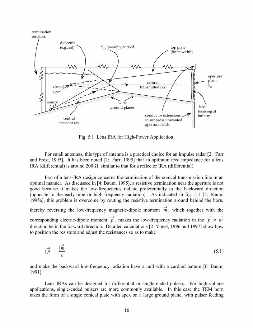
A lens IRA is basically a TEM horn with a lens at the aperture to straighten out thespherical TEM wave on the conical transmission line into a plane wave at the end (aperture).Having said that, there are many details to consider. Figure 5.1 gives a general picture of thistype of IRA. More concerning the lenses is given in Section 7. Section 4 of the bibliography (aswell as selected papers in other sections) gives a more extensive discussion of this type of IRA.

TEM horns have a long history [5: Baum, 1967; 4: Shaubert, 1977; 4: Kanda, 1983] forvarious applications (EMP simulators, communications antennas, measurements). For IRAapplication, however, it is only in the limit of small divergence angle of the horn (or sufficientlylong horn for given aperture dimensions and desired narrow radiated pulse width) that a TEMhorn can be thought of as an IRA [4: Farr and Baum, 1992]. In general a lens is required tomake the antenna fields into a plane wave at the aperture.

16

terminationresistors

dielectric(e.g., oil) SB (possibly curved) top plate

(finite width)

centraltransmitted ray

apertureplaneSa

lensfocusing atinfinityconductor extensions

to suppress unwantedaperture fields

wideground planes

centralincident ray

virtualapex

-+

source

X

Fig. 5.1 Lens IRA for High-Power Application.

For small antennas, this type of antenna is a practical choice for an impulse radar [2: Farrand Frost, 1995]. It has been noted [2: Farr, 1995] that an optimum feed impedance for a lensIRA (differential) is around 200 Ω, similar to that for a reflector IRA (differential).

Part of a lens-IRA design concerns the termination of the conical transmission line in anoptimal manner. As discussed in [4: Baum, 1995], a resistive termination near the aperture is notgood because it makes the low-frequencies radiate preferentially in the backward direction(opposite to the early-time or high-frequency radiation). As indicated in fig. 5.1 [2: Baum,1995a], this problem is overcome by routing the resistive termination around behind the horn,

thereby reversing the low-frequency magnetic-dipole moment m→

, which together with the

corresponding electric-dipole moment p→

, makes the low-frequency radiation in the p m→ →

×direction be in the forward direction. Detailed calculations [2: Vogel, 1996 and 1997] show howto position the resistors and adjust the resistances so as to make

| | | |p mc

→→

= (5.1)

and make the backward low-frequency radiation have a null with a cardiod pattern [6, Baum,1991].

Lens IRAs can be designed for differential or single-ended pulsers. For high-voltageapplications, single-ended pulsers are more commonly available. In this case the TEM horntakes the form of a single conical plate with apex on a large ground plane, with pulser feeding

17

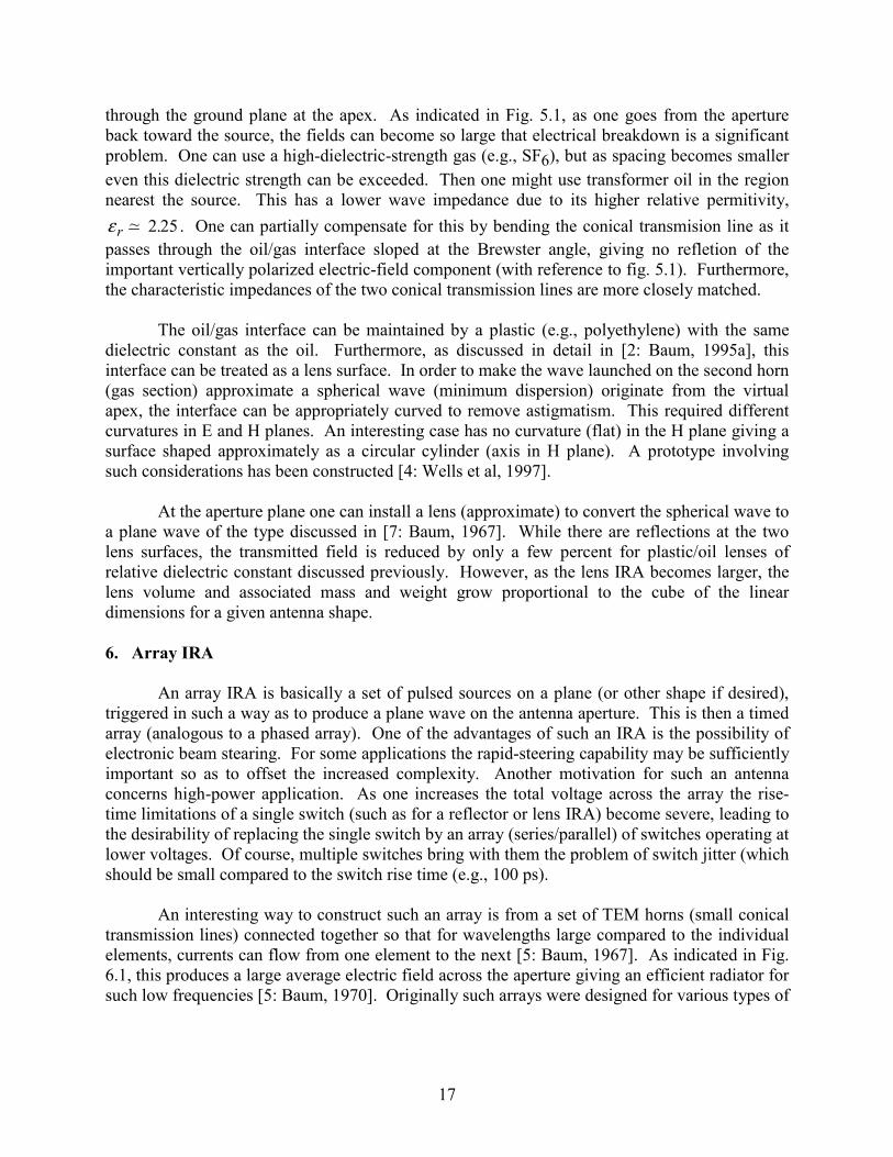
through the ground plane at the apex. As indicated in Fig. 5.1, as one goes from the apertureback toward the source, the fields can become so large that electrical breakdown is a significantproblem. One can use a high-dielectric-strength gas (e.g., SF6), but as spacing becomes smallereven this dielectric strength can be exceeded. Then one might use transformer oil in the regionnearest the source. This has a lower wave impedance due to its higher relative permitivity,ε r ~ .2 25. One can partially compensate for this by bending the conical transmision line as itpasses through the oil/gas interface sloped at the Brewster angle, giving no refletion of theimportant vertically polarized electric-field component (with reference to fig. 5.1). Furthermore,the characteristic impedances of the two conical transmission lines are more closely matched.

The oil/gas interface can be maintained by a plastic (e.g., polyethylene) with the samedielectric constant as the oil. Furthermore, as discussed in detail in [2: Baum, 1995a], thisinterface can be treated as a lens surface. In order to make the wave launched on the second horn(gas section) approximate a spherical wave (minimum dispersion) originate from the virtualapex, the interface can be appropriately curved to remove astigmatism. This required differentcurvatures in E and H planes. An interesting case has no curvature (flat) in the H plane giving asurface shaped approximately as a circular cylinder (axis in H plane). A prototype involvingsuch considerations has been constructed [4: Wells et al, 1997].

At the aperture plane one can install a lens (approximate) to convert the spherical wave toa plane wave of the type discussed in [7: Baum, 1967]. While there are reflections at the twolens surfaces, the transmitted field is reduced by only a few percent for plastic/oil lenses ofrelative dielectric constant discussed previously. However, as the lens IRA becomes larger, thelens volume and associated mass and weight grow proportional to the cube of the lineardimensions for a given antenna shape.

6. Array IRA

An array IRA is basically a set of pulsed sources on a plane (or other shape if desired),triggered in such a way as to produce a plane wave on the antenna aperture. This is then a timedarray (analogous to a phased array). One of the advantages of such an IRA is the possibility ofelectronic beam stearing. For some applications the rapid-steering capability may be sufficientlyimportant so as to offset the increased complexity. Another motivation for such an antennaconcerns high-power application. As one increases the total voltage across the array the rise-time limitations of a single switch (such as for a reflector or lens IRA) become severe, leading tothe desirability of replacing the single switch by an array (series/parallel) of switches operating atlower voltages. Of course, multiple switches bring with them the problem of switch jitter (whichshould be small compared to the switch rise time (e.g., 100 ps).

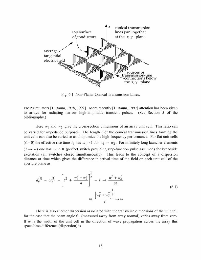
An interesting way to construct such an array is from a set of TEM horns (small conicaltransmission lines) connected together so that for wavelengths large compared to the individualelements, currents can flow from one element to the next [5: Baum, 1967]. As indicated in Fig.6.1, this produces a large average electric field across the aperture giving an efficient radiator forsuch low frequencies [5: Baum, 1970]. Originally such arrays were designed for various types of

18

top surfaceof conductors

averagetangentialelectric field

z conical transmissionlines join togetherat the x, y plane

sources ortransmission-line

connections belowthe x, y plane

Fig. 6.1 Non-Planar Conical Transmission Lines.

EMP simulators [1: Baum, 1978, 1992]. More recently [1: Baum, 1997] attention has been givento arrays for radiating narrow high-amplitude transient pulses. (See Section 5 of thebibliography.)

Here w1 and w2 give the cross-section dimensions of an array unit cell. This ratio canbe varied for impedance purposes. The length of the conical transmission lines forming theunit cells can also be varied so as to optimize the high-frequency performance. For flat unit cells( = 0) the effective rise time t1 has ct1 1~ for w w1 2~ . For infinitely long launcher elements

( → ∞ ) one has ct1 0~ (perfect switch providing step-function pulse assumed) for broadsideexcitation (all switches closed simultaneously). This leads to the concept of a dispersiondistance or time which gives the difference in arrival time of the field on each unit cell of theaperture plane as

d ct w w w w

w w

e e1 1 2 1

222

12 1

222

12

22

12

4 8b g b g= = + +L

NMM

OQPP − → +

+→ ∞

as

(6.1)

There is also another dispersion associated with the transverse dimensions of the unit cellfor the case that the beam angle θ1 (measured away from array normal) varies away from zero.If w is the width of the unit cell in the direction of wave propagation across the array thisspace/time difference (dispersion) is

19

d ct we e2 2

1b g b g b g= = sin θ (6.2)

If one wishes to scan the array over

0 1 1≤ ≤θ θ maxb g (6.3)

then this specifies

d we2

1,max max maxsinb g b g b g= FH IKθ (6.4)

where w can achieve a maximum value of

w w wmaxb g = +12

22

12 (6.5)

for particular choices of the aximuthal scan angle φ1. There is not much point in making

d de e1 2b g b g<< . One may choose these two to be comparable for an appropriate design

compromise.

With some choice of θ1maxb g and some desired small dispersion, the array-element (unit-

cell) dimensions are constrained. The length is limited so that a ray path from each source iskept within the horn. The cross-section dimensions are limited by w maxb g . For smallerdispersion or faster effective risetime one needs more array elements to fill a given array area.This represents a significant design tradeoff.

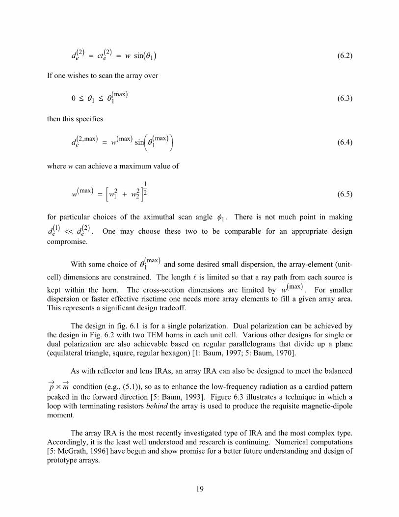
The design in fig. 6.1 is for a single polarization. Dual polarization can be achieved bythe design in Fig. 6.2 with two TEM horns in each unit cell. Various other designs for single ordual polarization are also achievable based on regular parallelograms that divide up a plane(equilateral triangle, square, regular hexagon) [1: Baum, 1997; 5: Baum, 1970].

As with reflector and lens IRAs, an array IRA can also be designed to meet the balanced

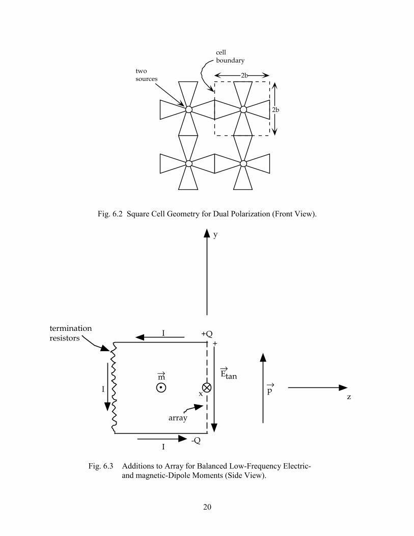
p m→ →× condition (e.g., (5.1)), so as to enhance the low-frequency radiation as a cardiod patternpeaked in the forward direction [5: Baum, 1993]. Figure 6.3 illustrates a technique in which aloop with terminating resistors behind the array is used to produce the requisite magnetic-dipolemoment.

The array IRA is the most recently investigated type of IRA and the most complex type.Accordingly, it is the least well understood and research is continuing. Numerical computations[5: McGrath, 1996] have begun and show promise for a better future understanding and design ofprototype arrays.

20

twosources

cellboundary

2b

2b

Fig. 6.2 Square Cell Geometry for Dual Polarization (Front View).

I +Q+

x

m→

array

-Q

terminationresistors

I

I

Etan

y

pz

→

→

Fig. 6.3 Additions to Array for Balanced Low-Frequency Electric-and magnetic-Dipole Moments (Side View).

21

7. Transient Lenses

Lenses can be included as parts of various types of IRA systems. Besides straighteningout the wave exiting a conical TEM waveguide (horn) as in a lens IRA (Section 5), lenses areused to redirect TEM waves (such as on coaxial waveguides) from one direction to another(bending lens) and/or between plane and spherical TEM waves. Note that the transient lensesused for this purpose are quite different, in general, from narrowband lenses (optical ormicrowave). In particular they need to have low dispersion for passing pulses with lowdistortion, and they often are constructed with transmission-line conductors passing throughthem and matching to TEM waveguides on both sides. In some cases the lenses and interfacesurfaces also need to withstand extremely high electric fields. These lenses come in two generalkinds to which we can refer as approximate and exact.

7.1 Approximate lenses

These are often constructed with some uniform dielectric such as polyethylene ortransformer oil. Transit times through the lens are preserved for the various ray paths betweenthe appropriate planar and/or spherical surfaces on both sides of the lens. However, somereflections at the lens surfaces are accepted in the interest of simplicity. Essentially thedifferential impedances along a duct [8: Baum and Stone, 1991] are not constant. However, fornot-too-large variations in the relative dielectric constant ε r (about 2.25 for polyethylene andtransformer oil) the performance is acceptable in some applications.

Section 7 of the Bibliography lists the various papers on this subject. In particular thedesign in [7: Baum et al, 1993] has been successfully incorporated in the launch onto the conicaltransmission line in a large reflector IRA [3: Giri et al, 1997; 3: Giri and Baum, 1977]. Otherdesigns are under study.

7.2 Exact lenses

Ideally, one would like to have the wave transitioned between TEM waveguides with nodistortion. How to do this, and the extent to which this can be done is the synthesis problem forsuch lenses. This can be viewed in two ways as discussed in [8: Baum and Stone, 1991].

One fundamental approach involves a differential geometric scaling from some simplerproblem (the formal problem) with a known TEM solution (say an inhomogeneous TEM planewave) in some as yet unspecified u1 , u2 , u3 orthogonal currilinear coordinate system (theformal system) initially regarded as Cartesian. Then regarding the un coordinates more

generally one asks what coordinate systems give acceptable permeability µ↔ →

( )r and permittivity

ε↔ →

( )r tensors to support the TEM wave (the real fields) in the now curved coordinates. Inaddition, this “lens region” generally needs to be matched to other regions with other TEMwaves (planar/spherical) on appropriate boundary surfaces.

22

A second approach uses the duct concept mentioned previously. Transit times betweenappropriate surfaces are made the same for all rays. A duct surrounding each ray is also made tohave the same impedance all along the ray (differential impedance matching). The first approachimplies the conditions mentioned above, but the second approach has allowed some solutionswith special kinds of anisotropic media involving metal sheets.

The earlier papers on this subject are summarized in [8: Baum and Stone, 1991]. Sincethen more progress has been made as indicated by the papers in Section 8 of the Bibliography.In particular in recent years research has concentrated on purely dielectric exacct lenses. This isrelated to the difficulty of constructing magnetic materials with frequency independent (andlossless) permeability over frequency ranges of interest (say 10s of MHz to 10s of GHz,depending on specific application). Various dielectrics are dispersionless (for practical purposesand over not-too-large lengths) over such frequencies. Of particular note is the discovery of aclass of solutions for a dielectric bending lens [8: Baum, 1996d]. This has the potential for beingquite practical and early experiments are reported [8: Bigelow and Farr, 1998].

8. Some Related Matters

Impulse-radiating antennas have been developed with practical applications in mindinvolving impulse-like fields in the far field. At the same time various investigators have beenexploring special kinds of pulsed electromagnetic waves for special properties (narrow beams,near field conditions, etc.). A selected set of references has been included for the reader inSection 10 of the Bibliography. One of the limitations of some of these waves is theirmathematical idealization involving the use of frequencies tending to infinity with significantamplitudes, a condition limited by real equipment. Nevertheless, these results can shed someinsight into what is (or is not) achievable in a pulse-radiating antenna.

9. Concluding Remarks

Recent years have shown much progress in the design of impulse-radiating antenna forvarious applications. There is ongoing research on multifunction IRAs [3: Farr et al, 1997] inwhich a single antenna handles multiple signals for communications, radar, and/or electronicwarfare. This involves multiple frequencies, possibly broadband pulses, polarization diversity,transmit and receive. Furthermore, the beamwidth may be variable by defocusing the antenna bymoving the feed point relative to the reflector, or by altering the reflector shape (in this case theantenna not being strictly an IRA). The array IRA also needs much more development forpractical implementation.

Besides strictly antenna issues, there are pulse-power issues for high-power IRAsoperating in pulse mode. Fast-rising high-voltage switching of pulses into the antenna can be ofthe order of 6 x 1015 V/s [2: Lehr et al, 1997]. To extend this performance one may investigatemultichannel switching or multiple switches (which now required small switch jitter) as in anarray (Section 6). In addition there are design problems in avoiding electrical breakdown on theantenna involving high-dielectric-strength materials. The exact lenses (Section 7.2) also need tobe realized in a good approximation using graded dielectrics which can also withstand highfields.

23

There are also mechanical issues requiring attention. Particularly near the feed point(apex of the conical transmission line) the conical conductors and connections can be quitedelicate considering their connection to large antenna structures which transmit large forces.These forces need to be relieved so as not to be transmitted to the apex. For some applicationsweight can be a problem and one needs to avoid massive dielectric lens-like structures in suchcases.

10. Bibliography

The various Notes cided in the bibliography are available from the authors or the editorC. E. Baum.

1. Reviews

F. J. Agee et al [1998], “Ultra-Wideband Transmitter Research,” IEEE Trans. Plasma Science,pp. 860–873.

C. E. Baum [1978], “EMP Simulators for Various Types of Nuclear EMP Environments: AnInterim Categorization,” IEEE Trans. Antennas and Propagation, and IEEE Trans. EMC, pp.35–53.

C. E. Baum [1992], “From the Electromagnetic Pulse to High-Power Electromagnetics,” Proc.IEEE, pp. 789–817.

C. E. Baum [1997], “Transient Arrays,” in C. E. Baum et al (eds.), Ultra-Wideband, Short-PulseElectromagnetics 3, New York, Plenum, pp. 129–138.

C. E. Baum and E. G. Farr [1993], “Impulse Radiating Antennas,” in H. Bertoni et al (eds.),Ultra-Wideband, Short-Pulse Electromagnetics, New York, Plenum, pp. 139–147.

E. G. Farr, C. E. Baum, and C. J. Buchenaur [1995], “Impulse Radiating Antennas, Part II,” inL. Carin and L. B. Felsen (eds.), Ultra-Wideband, Short-Pulse Electromagnetics 2, New York,Plenum, pp. 159–170.

E. G. Farr and C. E. Baum [1997], “Impulse Radiating Antennas, Part III,” in C. E. Baum et al(eds.) Ultra-Wideband, Short-Pulse Electromagnetics 3, New York, Plenum, pp. 43–56.

W. D. Prather et al [1997], “Ultrawide Band Source and Antennas: Present Technology, FutureChallenges,” in C. E. Baum et al (eds.), Ultra-Wideband, Short Pulse Electromagnetics 3, NewYork, Plenum, pp. 381–389.

I. D. Smith and H. Aslin [1978], “Pulsed Power for EMP Simulators,” IEEE Trans. Antennasand Propagation, and IEEE Trans. EMC, pp. 53–59.

24

2. Impulse Radiating Antennas (IRAs): General

C. E. Baum [1987], “Focused Aperture Antennas,” Sensor and Simulation Note 306, and Proc.1993 Antenna Applications Symposium, RL-TR-94-20, pp. 40–61.

C. E. Baum [1989], “Radiation of Impulse-Like Transient Fields,” Sensor and Simulation Note321.

C. E. Baum [1991], “Aperture Efficiencies for IRAs,” Sensor and Simulation Note 328.

C. E. Baum [1997], “A Symmetry Result for an Antenna on a Truncated Ground Plane,” Sensorand Simulation Note 415.

C. E. Baum [1997a], “Intermediate Field of an Impulse-Radiating Antenna,” Sensor andSimulation note 418.

C. J. Buchenauer, J. S. Tyo, and J. S. H. Schoenberg [1997], “Aperture Efficiencies of ImpulseRadiating Antennas,” Sensor and Simulation Note 421.

E. G. Farr and C. E. Baum [1993], “Radiation from Self-Reciprocal Apertures,” Sensor andSimulation Note 357, and [1995], in C. E. Baum and H. N. Kritikos (eds.), ElectromagneticSymmetry, Philadelphia, Taylor & Francis, pp. 281–308.

E. G. Farr and C. E. Baum [1995], “Impulse Radiating Antennas with Two Refracting ReflectingSurfaces,” Sensor and Simulation Note 379.

E. G. Farr and C. J. Buchenauer [1994], “Experimental Validation of IRA Models,” Sensor andSimulation Note 364.

E. G. Farr and C. A. Frost [1995], “Compact Ultra-Short Pulse Fuzing Antenna Design andMeasurements,” Sensor and Simulation Note 380.

E. G. Farr and C. A. Frost [1996], “Development of a Reflector IRA and a Solid Dielectric LensIRA, Part I: Design, predictions, and Construction,” Sensor and Simulation Note 396.

E. G. Farr and C. A. Frost [1996a], “Development of a Reflector IRA and a Solid Dielectric LensIRA, Part II: Antenna Measurements and Signal processing,” Sensor and Simulation Note 401.

D. V. Giri, [1996], “Propagation of Impulse-Like Waveforms through the Ionosphere Modelledby a Cold Plasma,” Theoretical Note 366.

E. Heyman and T. Melamed [1994], “Certain Considerations in Aperture Synthesis ofUltrawideband/Short-Pulse Radiation,” IEEE Trans. Antennas and Propagation, pp. 518−525.

J. M. Lehr, C. E. Baum, and W. D. Prather [1997], “Fundamental Physical Considerations forUltrafast Spark Gap Switching,” Switching Note 28.

25

S. P. Skulkin and V. I. Turchin [1994], “Radiation of Nonsinusoidal Waves by ApertureAntennas,” in D. J. Serafin, J. Ch. Bolomey, and D. Dupouy (eds.), Proc. EUROEM ’94,Bordeaux, France, pp. 1498–1504.

S. P. Skulkin [1997], “Transient Fields of Rectangular Aperture Antennas,” in C. E. Baum et al(eds.), Ultra-Wideband, Short-Pulse Electromagnetics 3, New York, Plenum press, pp. 57–63.

J. S. Tyo [1998, “Estimating the Optimum Aperture for Maximizing Prompt ApertureEfficiency in an IRA,” Sensor and Simulation Note 422.

3. Reflector IRA

C. E. Baum [1991], “Configurations of TEM Feed for an IRA,” Sensor and Simulation Note 327.

C. E. Baum [1997], “Some Topics Concerning Feed Arms of Reflector IRAs,” Sensor andSimulation Note 414.

C. E. Baum [1995], “Variations on the Impulse-Radiating-Antenna Theme,” Sensor andSimulation Note 378.

W. S. Bigelow and E. G. Farr [1997], “Design of a Feed-Point Lens with Offset Inner Conductorfor a Half Reflector IRA with F/D Greater than 0.25,” Sensor and Simulation Note 410.

W. S. Bigelow and E. G. Farr [1996], “Design Optimization of Feed-Point Lenses for HalfReflector IRAs,” Sensor and Simulation Not 400.

L. H. Bowen and E. G. Farr [1998], “E-Field measurements for a 1 Meter Diameter Half IRA,”Sensor and Simulation Note 419.

H.-T. Chou, P. H. Pathak, and P. R. Rousseau [1997], “Analytical Solution for Early-TimeTransient Radiation from Pulse-Excited Parabolic Reflector Antennas,” IEEE Trans. Antennasand Propagation, pp. 829–836.

C. Courtney et al [1995], “Measurement and Characterization of the Impulse RadiatingAntenna,” Prototype IRA Memo 5.

E. G. Farr [1991], “Analysis of the Impulse Radiating Antenna,” Sensor and Simulation Note329.

E. G. Farr [1993], “Optimizing the Feed Impedance of Impulse Radiating Antennas, Part I:Reflector IRAs,” Sensor and Simulation Note 354.

E. G. Farr and C. E. Baum [1992], “Prepulse Associated with the TEM Feed of an ImpulseRadiating Antenna,” Sensor and Simulation note 337.

E. G. Farr and C. E. Baum [1993], “The Radiation Pattern of Reflector Impulse RadiatingAntennas: Early-Time Response,” Sensor and Simulation Note 358.

26

E. G. Farr, C. E. Baum, and W. D. Prather [1997], “Multifunction Impulse Radiating Antennas:Theory and Experiment,” Sensor and Simulation Note 413.

E. G. Farr and G. D. Sower [1995], “Design Principles of Half Impulse Radiating Antennas,”Sensor and Simulation note 390.

D. V. Giri [1995], “Radiated Spectra of Impulse Radiating Antennas (IRAs),” Sensor andSimulation Note 386.

D. V. Giri and C. E. Baum [1994], “Reflector IRA Design and Boresight Temporal Waveforms,”Sensor and Simulation Note 365.

D. V. Giri and C. E. Baum [1997], “Temporal and Spectral Radiation on Boresight of a ReflectorType of Impulse Radiating Antenna (IRA),” in C. E. Baum et al (eds.), Ultra-Wideband, Short-Pulse Electromagnetics 3, New York, Plenum, pp. 65–72.

D. V. Giri and S. Y Chu [1992], “On the Low-Frequency Electric Dipole Moment of ImpulseRadiating Antennas (IRA),” Sensor and Simulation Note 346.

D. V. Giri et al [1995], “A Reflector Antenna for Radiating Impulse-Like Waveforms,” Sensorand Simulation Note 382.

D. V. Giri et al [1997], “Design, Fabrication, and Testing of a Paraboloidal Reflector Antennaand Pulser System for Impulse-Like Waveforms,” IEEE Trans. Plasma Science, pp. 318–326.

O. V. Mikheev et al [1997], “New Method for Calculating Pulse Radiation from an Antenna witha Reflector,” IEEE Trans. EMC, p. 48–54.

K. Min and M. Willis, Jr. [1997], “Dense Media Penetrating Radar,” in C. E. Baum et al (eds.),Ultra-Wideband, Short-Pulse Electromagnetics 3, New York, Plenum press, pp. 423–430.

Y. Rahmat-Samii [1992], “Analysis of Blockage Effects on TEM-Fed Paraboloidal ReflectorAntennas,” Sensor and Simulation Note 347.

Y. Rahmat-Samii and D. W. Duan [1995], “Axial Field of a TEM-Fed UWB Reflector Antenna:PO/PTD Construction,” in L. Carin and L. B. Felsen, Ultra-Wideband, Short-PulseElectromagnetics 2, New York, Plenum, pp. 171–186.

Y. Rahmat-Samii and D. V. Giri [1992], “Analysis of Blockage Effects on TEM-FedParaboloidal Antennas (Part II: TEM Horn Illumination),” Sensor and Simulation Note 349.

S. P. Skulkin and V. I. Turchin [1997], “Transient Fields of Parabolic Reflector Antennas,” in C.E. Baum et al (eds.), Ultra-Wideband, Short-Pulse Electromagnetics 3, New York, PlenumPress, pp. 81–87.

G. E. Sower et al [1998], “Design for Half Impulse Radiating Antennas: Lens material Selectionand Scale-Model Testing,” Measurement Note 54.

27

4. Lens IRA (Including TEM Horn)

J. F. Aurand [1997], “A TEM-Horn Antenna with Dielectric lens for Fast Impulse Response,” inC. E. Baum et al (eds.), Ultra-Wideband, Short-Pulse Electromagnetics 3, new York, Plenum,pp. 113–120.

C. E. Baum [1995], “Low-Frequency-Compensated TEM Horn,” Sensor and Simulation Note377.

C. E. Baum [1995a], “Brewster-Angle Interface Between Flat-Plate Conical TransmissionLines,” Sensor and Simulation Note 389.

E. G. Farr and C. E. Baum [1992], “A Simple Model of Small-Angle TEM Horns”, Sensor andSimulation Note 340.

E. G. Farr [1994], “Off-Boresight Field of a Lens IRA,” Sensor and Simulation Note 370.

E. G. Farr [1995], “Optimization of the Feed Impedance of Impulse Radiating Antennas, Part II:TEM Horns and Lens IRAs,” Sensor and Simulation Note 384.

E. G. Farr, G. D. Sower, L. M. Atchley, and D. E. Ellibee [1998], “Design and Fabrication of anUltra-Wideband High-Power Zipper Balun and Antenna,” Measurement Note 53.

M. Kanda [1983], “Time Domain Sensors for Radiated Impulsive Measurements,” IEEE Trans.Antennas and Propagation, pp. 438–444.

M. A. Morgan and R. Clark Robertson [1997], “Optimized TEM Horn Impulse ReceivingAntenna,” in C. E. Baum et al (eds.), Ultra-Wideband, Short-Pulse Electromagnetics 3, NewYork, Plenum Press, pp. 121–128.

R. C. Robertson and M. A. Morgan [1995], “Ultra-Wideband Impulse Receiving AntennaDesign and Evaluation,” in L. Carin and L. B. Felsen (eds.), Ultra-Wideband, Short-PulseElectromagnetics 3, new York, Plenum press, pp. 179–186.

D. H. Shaubert [1977], “Measurement of the Impulse Response of Communication Antennas,”Harry Diamond Laboratories Technical Report, HDL-TR-1832.

D. H. Shaubert, A. R. Sindoris, and F. G. Farrar [1976], “A Measurement Technique forDetermining the Time-Domain Voltage Response of UHF Antennas to EMP Excitation,” HarryDiamond Laboratories Technical Report, HDL-TR-1778.

J. S. Tyo, C. J. Buchenauer, and J. S. H. Schoenberg [1998], “Use of Isorefractive Media toImprove Prompt Aperture Efficiency in a lens IRA,” IEEE Trans. Antennas and Propagation, pp.1114–1115.

M. H. Vogel [1996], “Design of the Low-Frequency Compensation of an Extreme-BandwidthTEM Horn and Lens IRA,” Sensor and Simulation Note 391.

28

M. H. Vogel [1997], “Design of the Low-Frequency Compensation of an Extreme-BandwidthTEM Horn and Lens IRA,” in C. E. Baum et al (eds.), Ultra-Wideband, Short-PulseElectromagnetics 3, New York, Plenum Press, pp. 97–105.

J. Wells, C. E. Baum, N. Keator, and W. D. Prather [1997], “A Radiating Structure Incorporatingan Extended Ground Plane and a Brewster Angle Window,” in C. E. Baum et al (eds.), Ultra-Wideband, Short-Pulse Electromagnetics 3, New York, Plenum press, pp. 107–112.

5. Array IRA

P. R. Barnes [1970], “Pulse Radiation by an Infinitely Long, perfectly Conducting, CylindricalAntenna in Free Space, Excited by a Finite Cylindrical Distributed Source Specified by theTangential Electric Field Associated with a Biconical Antenna,” Sensor and Simulation Note110.

C. E. Baum [1967], “The Conical Transmission Line as a Wave Launcher and Terminator for aCylindrical Transmission line,” Sensor and Simulation Note 31.

C. E. Baum [1969], “The Distributed Source for Launching Spherical Waves,” Sensor andSimulation Note 84.

C. E. Baum [1970], “Some Characteristics of Planar Distributed Sources for Radiating TransientPulses,” Sensor and Simulation Note 100.

C. E. Baum [1972], “General Principles for the Design of ATLAS I and II, Part IV: AdditionalConsiderations for the Design of Pulser Arrays,” Sensor and Simulation Note 146.

C. E. Baum [1972a], “General Principles for the Design of ATLAS I and II, part V: SomeApproximate Figures of Merit for Comparing the Waveforms launched by Imperfect PulserArrays onto TEM Transmission Lines,” Sensor and Simulation Note 148.

C. E. Baum [1973], “Early Time Performance at Large Distances of Periodic Planar Arrays ofPlanar Bicones with Sources Triggered in a Plane-Wave Sequence,” Sensor and Simulation Note184.

C. E. Baum [1988], “Coupled Transmission-Line Model of Periodic Array of Wave Launchers,”Sensor and Simulation Note 313.

C. E. Baum [1989], “Canonical Examples for High-Frequency Propagation on Unit Cell ofWave-Launcher Array,” Sensor and Simulation Note 317.

C. E. Baum [1993], “Timed Arrays for Radiating Impulse-Like Transient Fields,” Sensor andSimulation Note 361, and [1995], Proc. SPIE, Vol. 2485, pp. 168−174.

C. E. Baum [1994], “Self-Complementary Array Antennas,” Sensor and Simulation Note 374.

C. E. Baum and D. V. Giri [1985], “The Distributed Switch for Launching Spherical Waves,”Sensor and Simulation Note 289, and Proc. 1997 EMC Symposium, Zurich, pp. 205–212.

29

G. W. Carlisle [1968], “Matching the Impedance of Multiple Transitions to a Parallel-PlateTransmission Line,” Sensor and Simulation Note 54.

Y.-G. Chen et al [1986], “Design Procedures for Arrays which Approximate a DistributedSource at the Air-Earth Interface,” Sensor and Simulation Note 292.

Y.-G. Chen et al [1990], “Low Voltage Experiments Concerning a Section of a Pulser ArrayNear the Air-Earth Interface,” Sensor and Simulation Note 322.

T. M. Flanagan et al [1987], “A Wide-Bandwidth Electric-Field Sensor for Lossy Media,”Sensor and Simulation Note 297.

D. V. Giri [1989], “Impedance Matrix Characterization of an Incremental Length of a PeriodicArray of Wave Launchers,” Sensor and Simulation Note 316.

D. V. Giri [1989a], “A Family of Canonical Examples for High Frequency Propagation on UnitCell of Wave-Launcher Array,” Sensor and Simulation Note 318.

D. V. Giri and C. E. Baum [1987], “Early Time Performance at Large Distances of PeriodicArrays of Flat-Plate Conical Wave Launchers,” Sensor and Simulation Note 299.

N. Inagaki, Y. Isogai, and Y. Mushiake [1979], “Self-Complementary Antenna with PeriodicFeeding Points,” Trans. IECE, Vol. 62-B, No. 4, pp. 388–395, in Japanese. Translation NAIC-ID(RS) T-0506-95, 1995, National Air Intelligence Center.

T. K. Liu [1973], “Admittances and Fields of a Planar Array with Sources Excited in a PlaneWave Sequence,” Sensor and Simulation Note 186.

D. T. McGrath [1996], “Numerical Analysis of Planar Bicone Arrays,” Sensor and SimulationNote 403.

D. T. McGrath [1998], “Numerical Analyses of TEM Horn Arrays,” Sensor and Simulation Note420.

Z. L. Pine and F. M. Tesche [1972], “Pulse Radiation by an Infinite Cylindrical Antenna with aSource Gap with a Uniform Field,” Sensor and Simulation note 159.

6. Antenna Parameterization for Time-Domain Applications (Emphasizing Far Fields)

O. E. Allen, D. A. Hill, and A. R. Ondrejka [1993], “Time-Domain Antenna Characterizations,”IEEE Trans. EMC, pp. 339−346.

C. E. Baum [1968], “Some Limiting Low-Frequency Characterstics of a Pulse-RadiatingAntenna,” Sensor and Simulation Note 65.

C. E. Baum [1971], “Some Characteristics of Electric and Magnetic Dipole Antennas forRadiating Transient Pulses,” Sensor and Simulation Note 125.

C. E. Baum [1991], “General Properties of Antennas,” Sensor and Simulation Note 330.

30

C. E. Baum [1995], “Optimization of Transient Radiation,” Sensor and Simulation Note 376.

C. E. Baum, E. G. Farr, and C. A. Frost [1997], “Transient Gain of Antennas Related to theTraditional Continuous-Wave (CW) Definition of Gain,” Sensor and Simulation Note 412.

E. G. Farr and C. E. Baum [1992], “Extending the Definitions of Antenna Gain and RadiationPattern Into the Time Domain,” Sensor and Simulation Note 350.

D. Lamensdorf and L. Sasman [1994], “Baseband-Pulse-Antenna Techniques,” IEEE Antennasand Propagation Magazine, February, pp. 20−30.

R. E. McIntosh and J. E. Sarna [1982], “Bounds on the Optimum Performance of PlanarAntennas for Pulse Radiation,"”IEEE Trans. Antennas and Propagation, pp. 381−389.

D. M. Pozar, D. H. Shaubert, and R. E. McIntosh [1984] “The Optimum Transient Radiationfrom an Arbitrary Antenna,” IEEE Trans. Antennas and Propagation, pp. 633−640.

A. Shlivinski, E. Heyman, and R. Kastner [1997], “Antenna Characterization in the TimeDomain,” IEEE Trans. Antennas and Propagation, pp. 1140−1149.

F. M. Tesche [1996], “Some Considerations for the Design of Pulse-Radiating Antennas,”Sensor and Simulation Note 398.

A. D. Yaghjian and T. B. Hansen [1997],”Theorems on Time-Domain Far Fields,” in C. E.Baum et al (eds.) Ultra-Wideband, Short-Pulse Electromagnetics 3, New York, Plenum Press,pp. 165−176.

7. Transient Lenses: Approximate

C. E. Baum [1967], “A Lens Technique for Transitioning Waves Between Conical andCylindrical Transmission Lines,” Sensor and Simulation Note 32.

C. E. Baum [1995], “Steerable Lens Surface for Use with the IRA Class of Antennas,” Sensorand Simulation Note 387.

C. E. Baum, J. J. Sadler, and A. P. Stone [1995], “A Prolate Spheroidal Uniform Dielectric LensFeeding a Circular Coax,” Electromagnetics, pp. 223−241.

C. E. Baum, J. J. Sadler, and A. P Stone [1992], “Uniform Isotropic Dielectric Equal-TimeLenses for Matching Combinations of Plane and Spherical Waves,” Sensor and Simulation Note352.

C. E. Baum, J. J. Sadler, and A. P. Stone [1992], “Uniform Wedge Dielectric Lenses for Bendsin Circular Coaxial Transmission Lines,” Sensor and Simulation Note 356.

C. E. Baum, J. J. Sadler, and A. P. Stone [1993], “A Uniform Dielectric lens for launching aSpherical Wave into a Paraboloidal Reflector,” Sensor and Simulation Note 360.

31

C. E. Baum, J. J. Sadler, and A. P. Stone [1994], “Impedances of Coplanar Conical Plates in aUniform Dielectric lens and matching Conical Plates for Feeding a Paraboloidal Reflector,”Sensor and Simulation Note 372.

C. E. Baum, J. J. Sadler, and A. P. Stone [1997], “Coplanar Conical Plates in a UniformDielectric Lens with Matching Conical Plates for Feeding a Paraboloidal Reflector,” in C. E.Baum et al (eds.) Ultra-Wideband Short-Pulse Electromagnetics 3, New York, Plenum Press, pp.73−80.

E. G. Farr and C. E. Baum [1995], “Feed-Point Senses for Half Reflector IRAs,” Sensor andSimulation Note 385.

8. Transient Lenses: Exact

W. S. Bigelow and E. G. Farr [1998], “Minimizing Dispersion in a TEM Waveguide Bend by aLayered Approximation of a Graded Dielectric Material,” Sensor and Simulation Note 416.

C. E. Baum [1991], “Wedge Dielectric Lenses for TEM Waves Between Parallel Plates,” Sensorand Simulation Note 332.

C. E. Baum [1992], “Arrays of Parallel Conducting Sheets for Two-Dimensional E-PlaneBending lenses,” Sensor and Simulation Note 341.

C. E. Baum [1995], “Two-Dimensional Inhomogeneous Dielectric Lenses for E-Plane Bends ofTEM Waves Guided Between Perfectly Conducting Sheets,” Sensor and Simulation Note 388.

C. E. Baum [1996], “Dielectric Body-of-Revolution Lenses with Azimuthal Propagation,”Sensor and Simulation Note 393.

C. E. Baum [1996a], “Dielectric Jackets as Lenses and Application to Generalized Coaxes andBends in Coaxial Cables,” Sensor and Simulation Note 394.

C. E. Baum [1996b], “Azimuthal TEM Waveguides in Dielectric Media,” Sensor and SimulationNote 397.

C. E. Baum [1996c], “Discrete and Continuous E-Plane Bends in Parallel-Plate Waveguide,”Sensor and Simulation Note 399.

C. E. Baum [1996d], “Use of Generalized Inhomogeneous TEM Plane Waves in DifferentialGeometric Lens Synthesis,” Sensor and Simulation Note 405, and Proc. 1998 InternationalSymposium on Electromagnetic Theory, Thessaloniki, Greece, pp. 636−638.

C. E. Baum and A. P. Stone [1991], Transient Lens Synthesis: Differential Geometry inElectromagnetic Theory, Philadelphia, Taylor & Francis.

C. E. Baum and A. P. Stone [1993], “Transient Lenses for Transmission Systems and Antennas,”in H. Bertoni et al (eds.), Ultra-Wideband, Short-Pulse Electromagnetics, New York, PlenumPress, pp. 211−219.

32

C. E. Baum and A. P. Stone [in publication], “Synthesis of Purely Dielectric Transient Lenses,”in Ultra-Wideband, Short-Pulse Electromagnetics 4, New York, Plenum Press.

9. Fields from Circular-Disk Sources Focused at Infinity

C. E. Baum [1992], “Circular Aperture Antennas in Time Domain,” Sensor and Simulation Note351.

D. J. Blejer [1989], “On-Axis Transient Fields from a Uniform Circular Distribution of Electricor Magnetic Current,” PIERS Proc., pp. 362−363.

D. J. Blejer, R. C. Wittmann, and A. D. Yaghjian [1993], “On-Axis Fields From a CircularUniform Surface Current,” in H. Bertoni et al (eds.), Ultra-Wideband, Short-PulseElectromagnetics, New York, Plenum, pp. 285−292.

R. R. Rudduck and C.-L. Chen [1976], “New Plane Wave Spectrum Formulations for the Near-Fields of Circular and Strip Antennas,” IEEE Trans. Antennas and Propagation, pp. 438−449.

A. D. Yaghjian [1982], “Eficient Computation of Antenna Coupling and Fields Within the Near-Field Region,” IEEE Trans. Antennas and Propagation, pp. 113−128.

10. Related Matter: Special Kinds of Waves (Selected)

J. L. Brittingham [1983], “Focus Waves Modes in Homogeneous Maxwell’s Equations:Transverse Electric Mode,” J. Appl. Phys., pp. 1179−1189.

B. B. Godfrey [1989], “Diffraction-Free Microwave Propagation,” Sensor and Simulation Note320.

E. Heyman [1993], “Wavepacket Solutions of the Time-Dependent Wave Equation inHomogeneous and Inhomogeneous Media,” in H. Bertoni et al (eds.), Ultra-Wideband, Short-Pulse Electromagnetics, New York, Plenum Press, pp. 241−250.

E. Heyman and L. B. Felsen [1986], “Propagating Pulsed Beam Solutions by Complex SourceParameter Substitution,” IEEE Trans. Antennas and Propagation, pp. 1062−1065.

H. E. Moser and R. T. Prosser [1986], “Initial Conditions, Sources, and Currents for PrescribedTime-Dependent Acoustic and Electromagnetic Fields in three Dimensions, part I: The InverseInitial Value Problem. Acoustic and Electromagnetic “Bullets,’ Expanding Waves, andImploding Waves,” IEEE Trans. Antennas and Propagation, pp. 188-196.

T. T. Wu [1985], “Electromagnetic Missiles,” J. Appl. Phys., pp. 2370−2375.

J. Zhan [1990], “General and Sufficient Electromagnetic Missile Condition,” IEEE Trans. EMC,pp. 304−307.

R. W. Ziolkowski [1992], “Properties of Electromagnetic Beams Generated by Ultra-WideBandwidth Pulse-Driven Arrays,” IEEE Trans. Antennas and Propagation, pp. 888−905.

33

R. W. Ziolkowski [1993], “UltraWide Bandwidth, Multi-Derivative Electromagnetic Systems,”in H. Bertoni et al (eds.), Ultra-Wideband, Short-Pulse Electromagnetics, New York, PlenumPress, pp. 251−258.