Regularized M-estimators of the Covariance Matrix
174
Regularized M-estimators of the Covariance Matrix Esa Ollila Aalto University, Department of Signal Processing and Acoustics, Finland esa.ollila@aalto.fi http://signal.hut.fi/ ~ esollila/ Summer School, R¨ udesheim, Sep 22, 2016
Transcript of Regularized M-estimators of the Covariance Matrix
Regularized M-estimators of the CovarianceMatrix
Esa Ollila
Aalto University, Department of Signal Processing and Acoustics, [email protected] http://signal.hut.fi/~esollila/
Summer School, Rudesheim, Sep 22, 2016
Contents
Part A Regularized M -estimators of covariance:
M -estimation and geodesic (g-)convexity
Regularization via g-convex penalties
Penalty (tuning) parameter selection
Part B Applications
Regularized discriminant analysis
Radar detection
Optimal portfolio selection
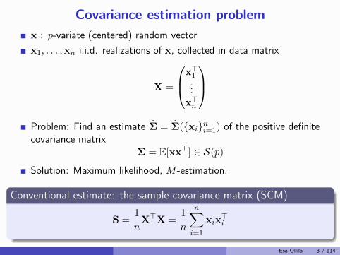
Covariance estimation problem
x : p-variate (centered) random vector
x1, . . . ,xn i.i.d. realizations of x, collected in data matrix
X =
x>1...
x>n
Problem: Find an estimate Σ = Σ({xi}ni=1) of the positive definitecovariance matrix
Σ = E[xx>] ∈ S(p)
Solution: Maximum likelihood, M -estimation.
Conventional estimate: the sample covariance matrix (SCM)
S =1
nX>X =
1
n
n∑
i=1
xix>i
Esa Ollila 3 / 114
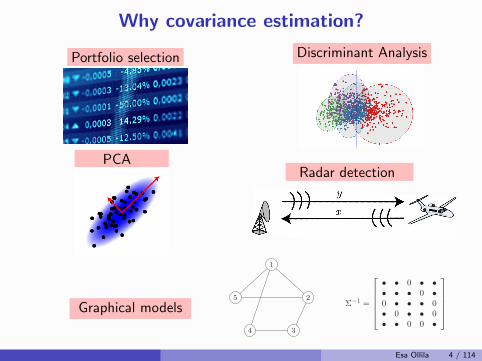
Why covariance estimation?
Portfolio selection Discriminant AnalysisThe Most Important Applications
graphical models clustering/discriminant analysis
PCAradar detection
Ilya Soloveychik (HUJI) Robust Covariance Estimation 15 / 47
PCA
The Most Important Applications
graphical models clustering/discriminant analysis
PCA radar detection
Ilya Soloveychik (HUJI) Robust Covariance Estimation 15 / 47
Radar detection
Graphical models
Gaussian graphical model
n-dimensional Gaussian vector
x = (x1, . . . , xn) ∼ N (0,Σ)
xi, xj are conditionally independent (given the rest of x) if
(Σ−1)ij = 0
modeled as undirected graph with n nodes; arc i, j is absent if (Σ−1)ij = 0
1
2
34
5Σ−1 =
• • 0 • •• • • 0 •0 • • • 0• 0 • • 0• • 0 0 •
1Esa Ollila 4 / 114
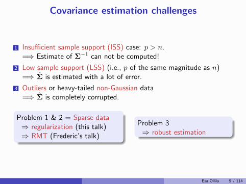
Covariance estimation challenges
1 Insufficient sample support (ISS) case: p > n.=⇒ Estimate of Σ−1 can not be computed!
2 Low sample support (LSS) (i.e., p of the same magnitude as n)=⇒ Σ is estimated with a lot of error.
3 Outliers or heavy-tailed non-Gaussian data=⇒ Σ is completely corrupted.
Problem 1 & 2 = Sparse data⇒ regularization (this talk)⇒ RMT (Frederic’s talk)
Problem 3⇒ robust estimation
Esa Ollila 5 / 114
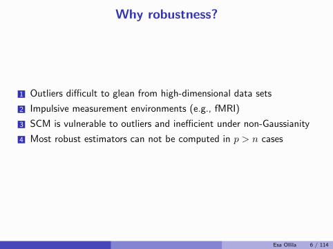
Why robustness?
1 Outliers difficult to glean from high-dimensional data sets
2 Impulsive measurement environments (e.g., fMRI)
3 SCM is vulnerable to outliers and inefficient under non-Gaussianity
4 Most robust estimators can not be computed in p > n cases
Esa Ollila 6 / 114
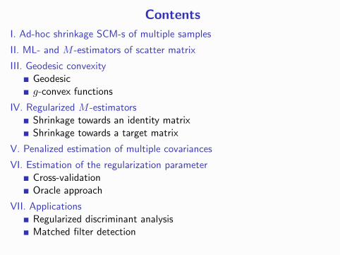
Contents
I. Ad-hoc shrinkage SCM-s of multiple samples
II. ML- and M -estimators of scatter matrix
III. Geodesic convexityGeodesicg-convex functions
IV. Regularized M -estimatorsShrinkage towards an identity matrixShrinkage towards a target matrix
V. Penalized estimation of multiple covariances
VI. Estimation of the regularization parameterCross-validationOracle approach
VII. ApplicationsRegularized discriminant analysisMatched filter detection

Acknowledgement
To my co-authors:
David E. TylerRutgers University
Ami WieselHebrew U. Jerusalem
Ilya SoloveychikHebrew U. Jerusalem
and many inspiring people working in this field:
Frederic Pascal, Teng Zhang, Lutz Dumbgen, Romain Couillet,Matthew R. McKay, Yuri Abramovich, Olivier Besson, MariaGreco, Fulvio Gini, Daniel Palomar, . . . . . .

I. Ad-hoc shrinkage SCM-s of multiple samples
II. ML- and M -estimators of scatter matrix
III. Geodesic convexity
IV. Regularized M -estimators
V. Penalized estimation of multiple covariances
VI. Estimation of the regularization parameter
VII. Applications
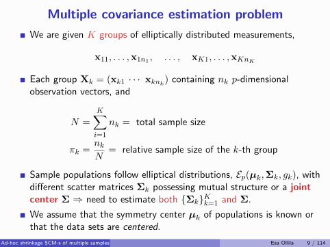
Multiple covariance estimation problem
We are given K groups of elliptically distributed measurements,
x11, . . . ,x1n1 , . . . , xK1, . . . ,xKnK
Each group Xk = (xk1 · · · xknk) containing nk p-dimensional
observation vectors, and
N =
K∑
i=1
nk = total sample size
πk =nkN
= relative sample size of the k-th group
Sample populations follow elliptical distributions, Ep(µk,Σk, gk), withdifferent scatter matrices Σk possessing mutual structure or a jointcenter Σ ⇒ need to estimate both {Σk}Kk=1 and Σ.
We assume that the symmetry center µk of populations is known orthat the data sets are centered.
Ad-hoc shrinkage SCM-s of multiple samples Esa Ollila 9 / 114
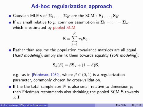
Ad-hoc regularization approach
Gaussian MLE-s of Σ1, . . . ,ΣK are the SCM-s S1, . . . ,SK
If nk small relative to p, common assumption is Σ1 = . . . = ΣK
which is estimated by pooled SCM
S =
K∑
k=1
πkSk.
Rather than assume the population covariance matrices are all equal(hard modeling), simply shrink them towards equality (soft modeling):
Sk(β) = βSk + (1− β)S,
e.g., as in [Friedman, 1989], where β ∈ (0, 1) is a regularizationparameter, commonly chosen by cross-validation.
If the the total sample size N is also small relative to dimension p,then Friedman recommends also shrinking the pooled SCM S towards∝ I.
Ad-hoc shrinkage SCM-s of multiple samples Esa Ollila 10 / 114
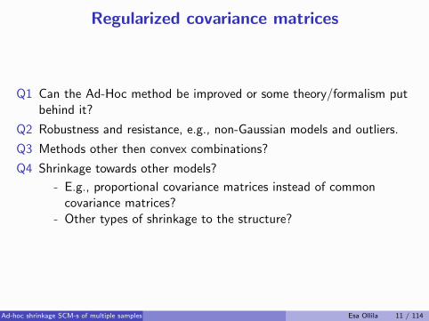
Regularized covariance matrices
Q1 Can the Ad-Hoc method be improved or some theory/formalism putbehind it?
Q2 Robustness and resistance, e.g., non-Gaussian models and outliers.
Q3 Methods other then convex combinations?
Q4 Shrinkage towards other models?
- E.g., proportional covariance matrices instead of commoncovariance matrices?
- Other types of shrinkage to the structure?
Ad-hoc shrinkage SCM-s of multiple samples Esa Ollila 11 / 114
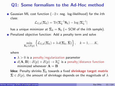
Q1: Some formalism to the Ad-Hoc method
Gaussian ML cost function (−2× neg. log-likelihood) for the kthclass:
LG,k(Σk) = Tr(Σ−1k Sk)− log |Σ−1k |
has a unique minimizer at Σk = Sk (= SCM of the kth sample).
Penalized objective function: Add a penalty term and solve
minΣk∈S(p)
{LG,k(Σk) + λ d(Σk, Σ)
}, k = 1, . . .K,
where
λ > 0 is a penalty/regularization parameterd(A,B) : S(p)× S(p)→ R+
0 is a penalty/distance functionminimized whenever A = B
Idea: Penalty shrinks Σk towards a fixed shrinkage target matrixΣ ∈ S(p), the amount of shrinkage depends on the magnitude of λ
Ad-hoc shrinkage SCM-s of multiple samples Esa Ollila 12 / 114
Q1: Some formalism to the Ad-Hoc method
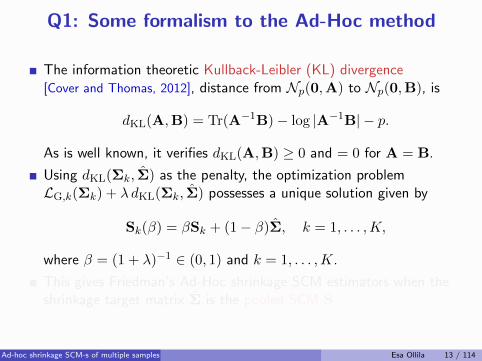
The information theoretic Kullback-Leibler (KL) divergence[Cover and Thomas, 2012], distance from Np(0,A) to Np(0,B), is
dKL(A,B) = Tr(A−1B)− log |A−1B| − p.
As is well known, it verifies dKL(A,B) ≥ 0 and = 0 for A = B.
Using dKL(Σk, Σ) as the penalty, the optimization problemLG,k(Σk) + λ dKL(Σk, Σ) possesses a unique solution given by
Sk(β) = βSk + (1− β)Σ, k = 1, . . . ,K,
where β = (1 + λ)−1 ∈ (0, 1) and k = 1, . . . ,K.
This gives Friedman’s Ad-Hoc shrinkage SCM estimators when theshrinkage target matrix Σ is the pooled SCM S
Ad-hoc shrinkage SCM-s of multiple samples Esa Ollila 13 / 114
Q1: Some formalism to the Ad-Hoc method
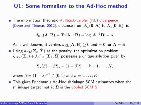
The information theoretic Kullback-Leibler (KL) divergence[Cover and Thomas, 2012], distance from Np(0,A) to Np(0,B), is
dKL(A,B) = Tr(A−1B)− log |A−1B| − p.
As is well known, it verifies dKL(A,B) ≥ 0 and = 0 for A = B.
Using dKL(Σk, Σ) as the penalty, the optimization problemLG,k(Σk) + λ dKL(Σk, Σ) possesses a unique solution given by
Sk(β) = βSk + (1− β)S , k = 1, . . . ,K,
where β = (1 + λ)−1 ∈ (0, 1) and k = 1, . . . ,K.
This gives Friedman’s Ad-Hoc shrinkage SCM estimators when theshrinkage target matrix Σ is the pooled SCM S
Ad-hoc shrinkage SCM-s of multiple samples Esa Ollila 13 / 114
Discussion
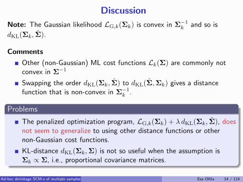
Note: The Gaussian likelihood LG,k(Σk) is convex in Σ−1k and so is
dKL(Σk, Σ).
Comments
Other (non-Gaussian) ML cost functions Lk(Σ) are commonly notconvex in Σ−1
Swapping the order dKL(Σk, Σ) to dKL(Σ,Σk) gives a distancefunction that is non-convex in Σ−1k .
Problems
The penalized optimization program, LG,k(Σk) + λ dKL(Σk, Σ), doesnot seem to generalize to using other distance functions or othernon-Gaussian cost functions.
KL-distance dKL(Σk,Σ) is not so useful when the assumption isΣk ∝ Σ, i.e., proportional covariance matrices.
Ad-hoc shrinkage SCM-s of multiple samples Esa Ollila 14 / 114
How about a robust Ad-hoc method?
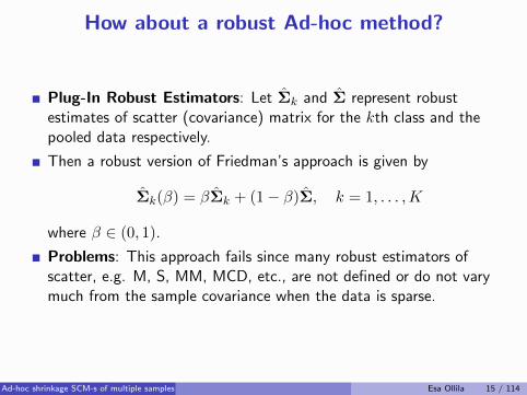
Plug-In Robust Estimators: Let Σk and Σ represent robustestimates of scatter (covariance) matrix for the kth class and thepooled data respectively.
Then a robust version of Friedman’s approach is given by
Σk(β) = βΣk + (1− β)Σ, k = 1, . . . ,K
where β ∈ (0, 1).
Problems: This approach fails since many robust estimators ofscatter, e.g. M, S, MM, MCD, etc., are not defined or do not varymuch from the sample covariance when the data is sparse.
Ad-hoc shrinkage SCM-s of multiple samples Esa Ollila 15 / 114
Our approach in this series of lectures
Regularization via jointly g-convex distance functions
Robust M-estimation (robust loss fnc downweights outliers)
Ad-hoc shrinkage SCM-s of multiple samples Esa Ollila 16 / 114

I. Ad-hoc shrinkage SCM-s of multiple samples
II. ML- and M -estimators of scatter matrix
III. Geodesic convexity
IV. Regularized M -estimators
V. Penalized estimation of multiple covariances
VI. Estimation of the regularization parameter
VII. Applications
References
R. A. Maronna (1976).Robust M-estimators of multivariate location and scatter.Ann. Stat., 5(1):51–67.
D. E. Tyler (1987).A distribution-free M-estimator of multivariate scatter.Ann. Stat., 15(1):234–251.
E. Ollila D. E. Tyler V. Koivunen, and H. V. Poor (2012).Complex elliptically symmetric distributions: survey, new results andapplications.IEEE Trans. Signal Processing, 60(11):5597 – 5625.
ML- and M -estimators of scatter matrix Esa Ollila 17 / 114
The cone of positive definite matrices S(p)A square matrix A is positive definite, denoted A � 0, if it issymmetric and satisfies
x>Ax > 0 ∀x 6= 0
Positive semidefinite (A � 0): x>Ax ≥ 0 ∀x.
A � 0 (� 0) if and only if its eigenvalues are positive (non-negative)
Eigenvalue decomposition (EVD) of A � 0;
A = EΛE> =
p∑
i=1
λieie>i
Λ = diag(λ1, . . . , λp) of positive eigenvalues
E =(e1 · · · ep
)orthonormal eigenvectors (E>E = I) as columns
S(p) := the set of all p× p positive definite matrices.
ML- and M -estimators of scatter matrix Esa Ollila 18 / 114
Elliptically symmetric (ES) distribution
x ∼ Ep(0,Σ, g) : p.d.f. is
f(x) ∝ |Σ|−1/2g(x>Σ−1x
)
Σ ∈ S(p), unknown positive definite p× p scatter matrix parameter.
g : R+0 → R+, fixed density generator.
When the covariance matrix exists: E[xx>] = Σ.
Example: Normal distribution Np(0,Σ) has p.d.f.
f(x) = π−p/2|Σ|−1/2 exp(− 1
2x>Σ−1x
).
Elliptical distribution with g(t) = exp(−t/2).
ML- and M -estimators of scatter matrix Esa Ollila 19 / 114
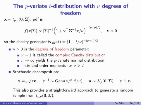
The p-variate t-distribution with ν degrees offreedom
x ∼ tp,ν(0,Σ): pdf is
f(x|Σ) ∝ |Σ|−1(
1 + x>Σ−1x/ν)−(p+ν)/2
, ν > 0
so the density generator is gν(t) = (1 + t/ν)−(p+ν)/2
ν > 0 is the degrees of freedom parameter:
ν = 1 is called the complex Cauchy distributionν →∞ yields the p-variate normal distributionfinite 2nd-order moments for ν > 2
Stochastic decomposition:
x =d
√τn, τ−1 ∼ Gam(ν/2, 2/ν), n ∼ Np(0,Σ), τ ⊥⊥ n.
This also provides a straightforward approach to generate a randomsample from tp,ν(0,Σ).
ML- and M -estimators of scatter matrix Esa Ollila 20 / 114

The maximum likelihood estimator (MLE)
{xi} iid∼ Ep(0,Σ, g), where n > p.
The MLE Σ ∈ S(p) minimizes the (−2/n) × log-likelihood fnc
L(Σ) =1
n
n∑
i=1
−2 ln f(xi|Σ) =1
n
n∑
i=1
ρ(x>i Σ−1xi)− ln |Σ−1|
where ρ(t) = −2 ln g(t) is the loss function.
Critical points are solutions to estimating equations
Σ =1
n
n∑
i=1
u(x>i Σ−1
xi)xix>i
where u(t) = ρ′(t) is the weight function.
MLE = ”an adaptively weighted sample covariance matrix”
ML- and M -estimators of scatter matrix Esa Ollila 21 / 114
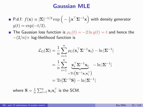
Gaussian MLE
P.d.f: f(x) ∝ |Σ|−1/2 exp(− 1
2x>Σ−1x)
with density generator
g(t) = exp(−t/2).
The Gaussian loss function is ρG(t) = −2 ln g(t) = t and hence the−(2/n)× log-likelihood function is
LG(Σ) =1
n
n∑
i=1
ρG(x>i Σ−1xi)− ln |Σ−1|
=1
n
n∑
i=1
x>i Σ−1xi︸ ︷︷ ︸=Tr(Σ−1xix>i
)− ln |Σ−1|
= Tr(Σ−1S
)− ln |Σ−1|
where S = 1n
∑ni=1 xix
>i is the SCM.
ML- and M -estimators of scatter matrix Esa Ollila 22 / 114
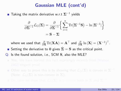
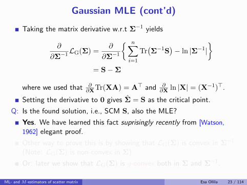
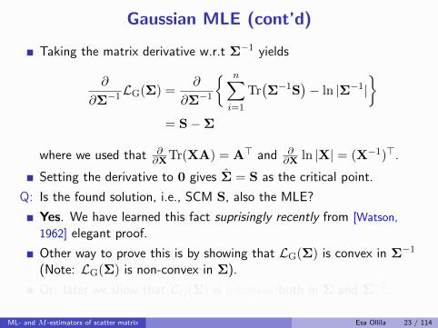
Gaussian MLE (cont’d)
Taking the matrix derivative w.r.t Σ−1 yields
∂
∂Σ−1LG(Σ) =
∂
∂Σ−1
{ n∑
i=1
Tr(Σ−1S
)− ln |Σ−1|
}
= S−Σ
where we used that ∂∂XTr(XA) = A> and ∂
∂X ln |X| = (X−1)>.
Setting the derivative to 0 gives Σ = S as the critical point.
Q: Is the found solution, i.e., SCM S, also the MLE?
Yes. We have learned this fact suprisingly recently from [Watson,
1962] elegant proof.
Other way to prove this is by showing that LG(Σ) is convex in Σ−1
(Note: LG(Σ) is non-convex in Σ).
Or: later we show that LG(Σ) is g-convex both in Σ and Σ−1.
ML- and M -estimators of scatter matrix Esa Ollila 23 / 114
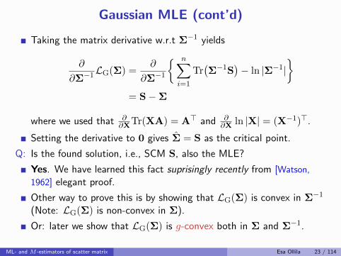
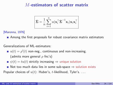
M-estimators of scatter matrix
Σ =1
n
n∑
i=1
u(x>i Σ−1
xi)xix>i
[Maronna, 1976]
Among the first proposals for robust covariance matrix estimators
Generalizations of ML-estimators:
u(t) = ρ′(t) non-neg., continuous and non-increasing.
(admits more general ρ fnc’s)
ψ(t) = tu(t) strictly increasing ⇒ unique solution
Not too much data lies in some sub-space ⇒ solution exists
Popular choices of u(t): Huber’s, t-likelihood, Tyler’s. . . .
ML- and M -estimators of scatter matrix Esa Ollila 24 / 114
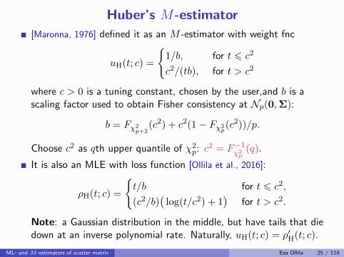
Huber’s M-estimator
[Maronna, 1976] defined it as an M -estimator with weight fnc
uH(t; c) =
{1/b, for t 6 c2
c2/(tb), for t > c2
where c > 0 is a tuning constant, chosen by the user,and b is ascaling factor used to obtain Fisher consistency at Np(0,Σ):
b = Fχ2p+2
(c2) + c2(1− Fχ2p(c2))/p.
Choose c2 as qth upper quantile of χ2p: c2 = F−1
χ2p
(q).
It is also an MLE with loss function [Ollila et al., 2016]:
ρH(t; c) =
{t/b for t 6 c2,
(c2/b)(
log(t/c2) + 1)
for t > c2.
Note: a Gaussian distribution in the middle, but have tails that diedown at an inverse polynomial rate. Naturally, uH(t; c) = ρ′H(t; c).
ML- and M -estimators of scatter matrix Esa Ollila 25 / 114
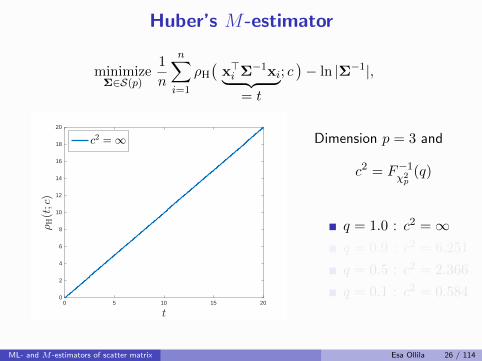
Huber’s M-estimator
minimizeΣ∈S(p)
1
n
n∑
i=1
ρH(
x>i Σ−1xi︸ ︷︷ ︸= t
; c)− ln |Σ−1|,
0 5 10 15 20
t
0
2
4
6
8
10
12
14
16
18
20
;H(t
;c)
c2 = 1 Dimension p = 3 and
c2 = F−1χ2p
(q)
q = 1.0 : c2 =∞q = 0.9 : c2 = 6.251
q = 0.5 : c2 = 2.366
q = 0.1 : c2 = 0.584
ML- and M -estimators of scatter matrix Esa Ollila 26 / 114
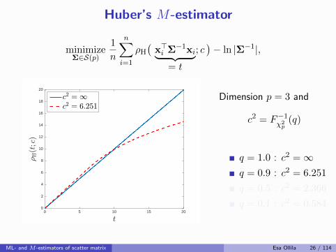
Huber’s M-estimator
minimizeΣ∈S(p)
1
n
n∑
i=1
ρH(
x>i Σ−1xi︸ ︷︷ ︸= t
; c)− ln |Σ−1|,
0 5 10 15 20
t
0
2
4
6
8
10
12
14
16
18
20
;H(t
;c)
c2 = 1c2 = 6:251
Dimension p = 3 and
c2 = F−1χ2p
(q)
q = 1.0 : c2 =∞q = 0.9 : c2 = 6.251
q = 0.5 : c2 = 2.366
q = 0.1 : c2 = 0.584
ML- and M -estimators of scatter matrix Esa Ollila 26 / 114
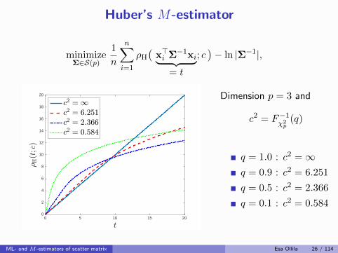
Huber’s M-estimator
minimizeΣ∈S(p)
1
n
n∑
i=1
ρH(
x>i Σ−1xi︸ ︷︷ ︸= t
; c)− ln |Σ−1|,
0 5 10 15 20
t
0
2
4
6
8
10
12
14
16
18
20
;H(t
;c)
c2 = 1c2 = 6:251c2 = 2:366c2 = 0:584
Dimension p = 3 and
c2 = F−1χ2p
(q)
q = 1.0 : c2 =∞q = 0.9 : c2 = 6.251
q = 0.5 : c2 = 2.366
q = 0.1 : c2 = 0.584
ML- and M -estimators of scatter matrix Esa Ollila 26 / 114
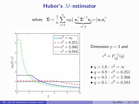
Huber’s M-estimator
solves Σ =1
n
n∑
i=1
uH(
x>i Σ−1
xi︸ ︷︷ ︸= t
; c)xix>i
t0 2 4 6 8 10
uH(t
;c)
0
1
2
3
4
5
6
c2 = 1c2 = 6:251c2 = 2:366c2 = 0:584
Dimension p = 3 and
c2 = F−1χ2p
(q)
• q = 1.0 : c2 =∞• q = 0.9 : c2 = 6.251• q = 0.5 : c2 = 2.366• q = 0.1 : c2 = 0.584
ML- and M -estimators of scatter matrix Esa Ollila 27 / 114
The MLE of tp,ν-distribution
Density generator of tp,ν(0,Σ) is gν(t) = (1 + t/ν)−12(ν+p).
M -estimator Σ based on the respective loss and weight function
ρν(t) = −2 ln gν(t) = (ν + p) ln(1 + t/ν)
uν(t) = ρ′ν(t) =ν + p
ν + t
is referred to as tνM -estimator.
Naturally an MLE when {xi}ni=1iid∼ tp,ν(0,Σ).
To obtain a Fisher consistent tνM -estimator Σ at Np(0,Σ), use ascaled loss function:
ρ∗ν(t) =1
bρν(t), b = {(ν + p)/p}E[χ2
p/(ν + χ2p)].
and respective scaled weight function u∗ν(t) = uν(t)/b,
ML- and M -estimators of scatter matrix Esa Ollila 28 / 114
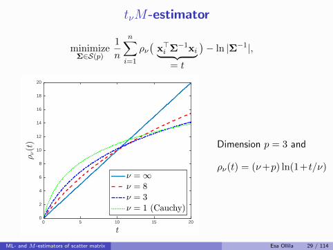
tνM-estimator
minimizeΣ∈S(p)
1
n
n∑
i=1
ρν(
x>i Σ−1xi︸ ︷︷ ︸= t
)− ln |Σ−1|,
t0 5 10 15 20
;8(t
)
0
2
4
6
8
10
12
14
16
18
20
8 = 18 = 88 = 38 = 1 (Cauchy)
Dimension p = 3 and
ρν(t) = (ν+p) ln(1+t/ν)
ML- and M -estimators of scatter matrix Esa Ollila 29 / 114
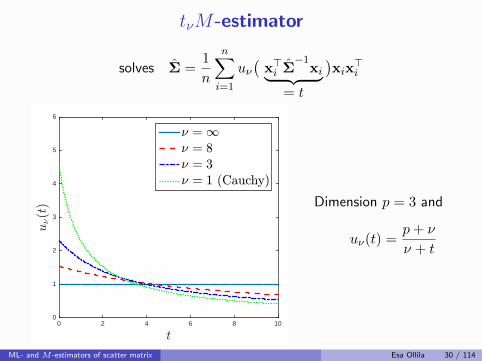
tνM-estimator
solves Σ =1
n
n∑
i=1
uν(
x>i Σ−1
xi︸ ︷︷ ︸= t
)xix>i
t0 2 4 6 8 10
u8(t
)
0
1
2
3
4
5
6
8 = 18 = 88 = 38 = 1 (Cauchy)
Dimension p = 3 and
uν(t) =p+ ν
ν + t
ML- and M -estimators of scatter matrix Esa Ollila 30 / 114
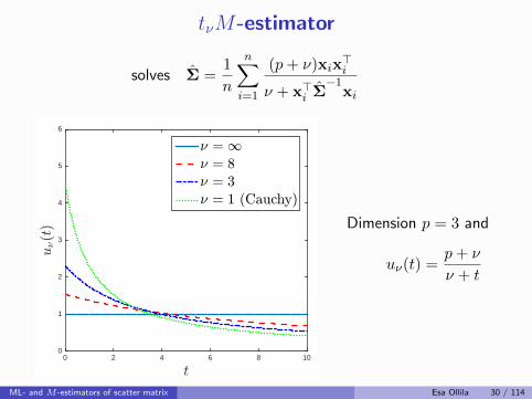
tνM-estimator
solves Σ =1
n
n∑
i=1
(p+ ν)xix>i
ν + x>i Σ−1
xi
t0 2 4 6 8 10
u8(t
)
0
1
2
3
4
5
6
8 = 18 = 88 = 38 = 1 (Cauchy)
Dimension p = 3 and
uν(t) =p+ ν
ν + t
ML- and M -estimators of scatter matrix Esa Ollila 30 / 114
Tyler’s M-estimator
Distribution-free M -estimator (under elliptical distributions) proposedin [Tyler, 1987].
Defined as a solution to
Σ =p
n
n∑
i=1
xix>i
x>i Σ−1
xi
⇒ so an M -estimator with Tyler’s weight fnc u(t) = ρ′(t) = p/t
Now it is also known that Σ ∈ S(p) minimizes the cost fnc
LT(Σ) =1
n
n∑
i=1
p ln(x>i Σ−1xi)︸ ︷︷ ︸ρ(t) = p ln t
− ln |Σ−1|
Note: not an MLE for any elliptical density, so ρ(t) 6= −2 ln g(t) !
Not convex in Σ ! . . . or in Σ−1
Maronna’s/Huber’s conditions does not apply.
ML- and M -estimators of scatter matrix Esa Ollila 31 / 114
Tyler’s M-estimator, cont’d
Σ =p
n
n∑
i=1
xix>i
x>i Σ−1
xi
Comments:
1 Limiting case of Huber’s M -estimator when c→ 0 and oftνM -estimator when ν → 0.
2 Minimum is a unique up to a positive scalar: if Σ is a minimum thenso is bΣ for any b > 0
⇒ Σ is a shape matrix estimator. We may choose a solution whichverifies |Σ| = 1.
3 A Fisher consistent estimator at Np(0,Σ) can be obtained by scaling
any minimum Σ by
b = Median{x>i Σ−1
xi; i = 1, . . . , n}/Median(χ2p).
This scaling is utilized in discriminant analysis later on.
ML- and M -estimators of scatter matrix Esa Ollila 32 / 114
Tyler’s M-estimator, cont’d
cΣ =p
n
n∑
i=1
xix>i
x>i (cΣ)−1xi
Comments:
1 Limiting case of Huber’s M -estimator when c→ 0 and oftνM -estimator when ν → 0.
2 Minimum is a unique up to a positive scalar: if Σ is a minimum thenso is bΣ for any b > 0
⇒ Σ is a shape matrix estimator. We may choose a solution whichverifies |Σ| = 1.
3 A Fisher consistent estimator at Np(0,Σ) can be obtained by scaling
any minimum Σ by
b = Median{x>i Σ−1
xi; i = 1, . . . , n}/Median(χ2p).
This scaling is utilized in discriminant analysis later on.
ML- and M -estimators of scatter matrix Esa Ollila 32 / 114
Tyler’s M-estimator, cont’d
Σ =p
n
n∑
i=1
xix>i
x>i Σ−1
xi
Comments:
1 Limiting case of Huber’s M -estimator when c→ 0 and oftνM -estimator when ν → 0.
2 Minimum is a unique up to a positive scalar: if Σ is a minimum thenso is bΣ for any b > 0
⇒ Σ is a shape matrix estimator. We may choose a solution whichverifies |Σ| = 1.
3 A Fisher consistent estimator at Np(0,Σ) can be obtained by scaling
any minimum Σ by
b = Median{x>i Σ−1
xi; i = 1, . . . , n}/Median(χ2p).
This scaling is utilized in discriminant analysis later on.
ML- and M -estimators of scatter matrix Esa Ollila 32 / 114
Tyler’s M-estimator as MLE
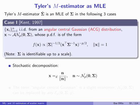
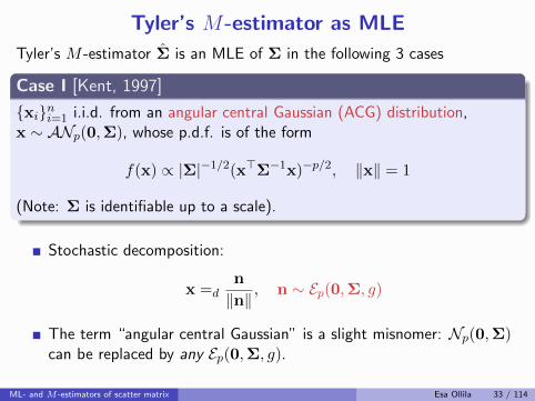
Tyler’s M -estimator Σ is an MLE of Σ in the following 3 cases
Case I [Kent, 1997]
{xi}ni=1 i.i.d. from an angular central Gaussian (ACG) distribution,x ∼ ANp(0,Σ), whose p.d.f. is of the form
f(x) ∝ |Σ|−1/2(x>Σ−1x)−p/2, ‖x‖ = 1
(Note: Σ is identifiable up to a scale).
Stochastic decomposition:
x =dn
‖n‖ , n ∼ Np(0,Σ)
The term “angular central Gaussian” is a slight misnomer: Np(0,Σ)can be replaced by any Ep(0,Σ, g).
ML- and M -estimators of scatter matrix Esa Ollila 33 / 114
Tyler’s M-estimator as MLE
Tyler’s M -estimator Σ is an MLE of Σ in the following 3 cases
Case I [Kent, 1997]
{xi}ni=1 i.i.d. from an angular central Gaussian (ACG) distribution,x ∼ ANp(0,Σ), whose p.d.f. is of the form
f(x) ∝ |Σ|−1/2(x>Σ−1x)−p/2, ‖x‖ = 1
(Note: Σ is identifiable up to a scale).
Stochastic decomposition:
x =dn
‖n‖ , n ∼ Ep(0,Σ, g)
The term “angular central Gaussian” is a slight misnomer: Np(0,Σ)can be replaced by any Ep(0,Σ, g).
ML- and M -estimators of scatter matrix Esa Ollila 33 / 114
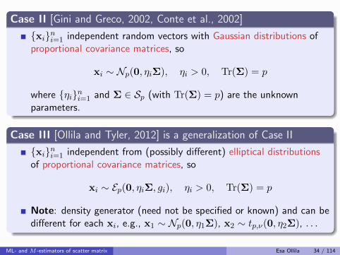
Case II [Gini and Greco, 2002, Conte et al., 2002]
{xi}ni=1 independent random vectors with Gaussian distributions ofproportional covariance matrices, so
xi ∼ Np(0, ηiΣ), ηi > 0, Tr(Σ) = p
where {ηi}ni=1 and Σ ∈ Sp (with Tr(Σ) = p) are the unknownparameters.
Case III [Ollila and Tyler, 2012] is a generalization of Case II
{xi}ni=1 independent from (possibly different) elliptical distributionsof proportional covariance matrices, so
xi ∼ Ep(0, ηiΣ, gi), ηi > 0, Tr(Σ) = p
Note: density generator (need not be specified or known) and can bedifferent for each xi, e.g., x1 ∼ Np(0, η1Σ), x2 ∼ tp,ν(0, η2Σ), . . .
ML- and M -estimators of scatter matrix Esa Ollila 34 / 114
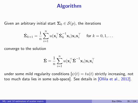
Algorithm
Given an arbitrary initial start Σ0 ∈ S(p), the iterations
Σk+1 =1
n
n∑
i=1
u(x>i Σ−1k xi)xix
>i for k = 0, 1, . . .
converge to the solution
Σ =1
n
n∑
i=1
u(x>i Σ−1
xi)xix>i
under some mild regularity conditions [ψ(t) = tu(t) strictly increasing, nottoo much data lies in some sub-space]. See details in [Ollila et al., 2012].
ML- and M -estimators of scatter matrix Esa Ollila 35 / 114
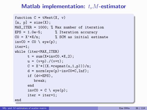
Matlab implementation: tνM-estimator
function C = tMest(X, v)
[n, p] = size(X);
MAX_ITER = 1000; % Max number of iteration
EPS = 1.0e-5; % Iteration accuracy
C0 = X’*X/n; % SCM as initial estimate
invC0 = C0 \ eye(p);
iter=1;
while (iter<MAX_ITER)
t = sum(X*invC0.*X,2);
u = (v+p)./(v+t);
C = X’*((X.*repmat(u,1,p)))/n;
d = norm(eye(p)-invC0*C,Inf);
if (d<=EPS),
break;
end
invC0 = C \ eye(p);
iter = iter+1;
end
ML- and M -estimators of scatter matrix Esa Ollila 36 / 114
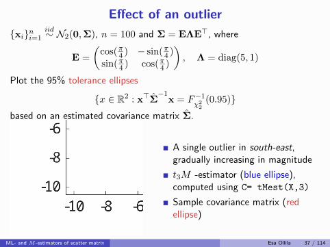
Effect of an outlier
{xi}ni=1iid∼ N2(0,Σ), n = 100 and Σ = EΛE>, where
E =
(cos(π4 ) − sin(π4 )sin(π4 ) cos(π4 )
), Λ = diag(5, 1)
Plot the 95% tolerance ellipses
{x ∈ R2 : x>Σ−1
x = F−1χ22
(0.95)}based on an estimated covariance matrix Σ.
A single outlier in south-east,gradually increasing in magnitude
t3M -estimator (blue ellipse),computed using C= tMest(X,3)
Sample covariance matrix (redellipse)
ML- and M -estimators of scatter matrix Esa Ollila 37 / 114
I. Ad-hoc shrinkage SCM-s of multiple samples
II. ML- and M -estimators of scatter matrix
III. Geodesic convexityGeodesicg-convex functions
IV. Regularized M -estimators
V. Penalized estimation of multiple covariances
VI. Estimation of the regularization parameter
VII. Applications
References
Wiesel, A. (2012a).Geodesic convexity and covariance estimation.IEEE Trans. Signal Process., 60(12):6182–6189.
Zhang, T., Wiesel, A., and Greco, M. S. (2013).Multivariate generalized Gaussian distribution: Convexity andgraphical models.IEEE Trans. Signal Process., 61(16):4141–4148.
Bhatia, R. (2009).Positive definite matrices.Princeton University Press.
Geodesic convexity Esa Ollila 38 / 114
From Euclidean convexity to Riemannian convexity
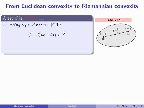
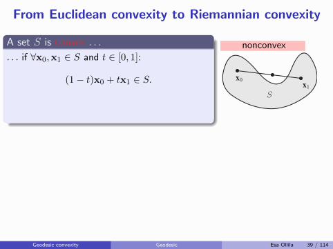
A set S is convex . . .
. . . if ∀x0,x1 ∈ S and t ∈ [0, 1]:
(1− t)x0 + tx1 ∈ S.
. . . if together with x0 and x1, it contains theshortest path (goedesic) connecting them
convex
x1
S
t = 0
x0
12t =
t = 1
What is Convexity?
We say that a set is convex if
∀ x, y ∈ S and ∀ t ∈ [0,1] ∶ tx + (1 − t)y ∈ S,or, if together with x and y, it contains the shortest path connecting them.
In Euclidean metric with the norm
∥x∥ = √∑j
x2j ,
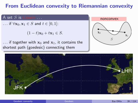
the shortest curves are line segments, butif we change metric, the notion ofconvexity changes, since the “shortestpath” (called geodesic) alters.
Ilya Soloveychik (HUJI) Robust Covariance Estimation 22 / 47
Geodesic convexity Geodesic Esa Ollila 39 / 114
From Euclidean convexity to Riemannian convexity
A set S is convex . . .
. . . if ∀x0,x1 ∈ S and t ∈ [0, 1]:
(1− t)x0 + tx1 ∈ S.
. . . if together with x0 and x1, it contains theshortest path (goedesic) connecting them
nonconvex
x0x1
S
What is Convexity?
We say that a set is convex if
∀ x, y ∈ S and ∀ t ∈ [0,1] ∶ tx + (1 − t)y ∈ S,or, if together with x and y, it contains the shortest path connecting them.
In Euclidean metric with the norm
∥x∥ = √∑j
x2j ,
the shortest curves are line segments, butif we change metric, the notion ofconvexity changes, since the “shortestpath” (called geodesic) alters.
Ilya Soloveychik (HUJI) Robust Covariance Estimation 22 / 47
Geodesic convexity Geodesic Esa Ollila 39 / 114
Euclidean convexity
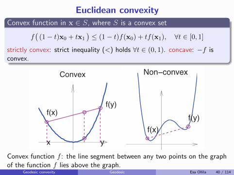
Convex function in x ∈ S, where S is a convex set
f(
(1− t)x0 + tx1
)≤ (1− t)f(x0) + tf(x1), ∀t ∈ [0, 1]
strictly convex: strict inequality (<) holds ∀t ∈ (0, 1). concave: −f isconvex.
x
f(x)
y
f(y)
Convex
f(y)
f(x)
f(y)
Non−convex
Convex function f : the line segment between any two points on the graphof the function f lies above the graph.
Geodesic convexity Geodesic Esa Ollila 40 / 114
Basic examples
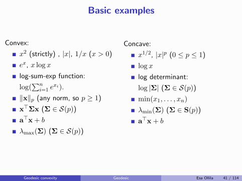
Convex:
x2 (strictly) , |x|, 1/x (x > 0)
ex, x log x
log-sum-exp function:
log(∑n
i=1 exi).
‖x‖p (any norm, so p ≥ 1)
x>Σx (Σ ∈ S(p))
a>x + b
λmax(Σ) (Σ ∈ S(p))
Concave:
x1/2, |x|p (0 ≤ p ≤ 1)
log x
log determinant:
log |Σ| (Σ ∈ S(p))
min(x1, . . . , xn)
λmin(Σ) (Σ ∈ S(p))
a>x + b
Geodesic convexity Geodesic Esa Ollila 41 / 114
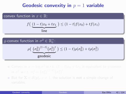
Geodesic convexity in p = 1 variable
convex function in x ∈ R:
f(x) = ρ(ex), x = log(σ2)
f(
(1− t)x0 + tx1︸ ︷︷ ︸line
)≤ (1− t)f(x0) + tf(x1)
g-convex function in σ2 ∈ R+0 :
ρ(σ2) = f(log σ2), σ2 = ex
ρ( (σ20)(1−t)(
σ21)t
︸ ︷︷ ︸geodesic
)≤ (1− t)ρ(σ20) + tρ(σ21)
Convex in x = log σ2 w.r.t. (1− t)x0 + tx1 is equivalent to g-convex
in σ2 w.r.t. σ2t =(σ20)(1−t)(
σ21)t
.
But for Σ ∈ S(p), p 6= 1, the solution is not a simple change ofvariables.
Geodesic convexity Geodesic Esa Ollila 42 / 114
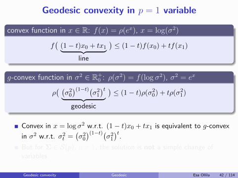
Geodesic convexity in p = 1 variable
convex function in x ∈ R: f(x) = ρ(ex), x = log(σ2)
f(
(1− t)x0 + tx1︸ ︷︷ ︸line
)≤ (1− t)f(x0) + tf(x1)
g-convex function in σ2 ∈ R+0 : ρ(σ2) = f(log σ2), σ2 = ex
ρ( (σ20)(1−t)(
σ21)t
︸ ︷︷ ︸geodesic
)≤ (1− t)ρ(σ20) + tρ(σ21)
Convex in x = log σ2 w.r.t. (1− t)x0 + tx1 is equivalent to g-convex
in σ2 w.r.t. σ2t =(σ20)(1−t)(
σ21)t
.
But for Σ ∈ S(p), p 6= 1, the solution is not a simple change ofvariables.
Geodesic convexity Geodesic Esa Ollila 42 / 114
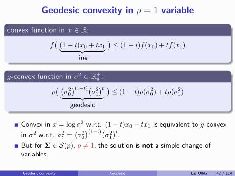
Geodesic convexity in p = 1 variable
convex function in x ∈ R:
f(x) = ρ(ex), x = log(σ2)
f(
(1− t)x0 + tx1︸ ︷︷ ︸line
)≤ (1− t)f(x0) + tf(x1)
g-convex function in σ2 ∈ R+0 :
ρ(σ2) = f(log σ2), σ2 = ex
ρ( (σ20)(1−t)(
σ21)t
︸ ︷︷ ︸geodesic
)≤ (1− t)ρ(σ20) + tρ(σ21)
Convex in x = log σ2 w.r.t. (1− t)x0 + tx1 is equivalent to g-convex
in σ2 w.r.t. σ2t =(σ20)(1−t)(
σ21)t
.
But for Σ ∈ S(p), p 6= 1, the solution is not a simple change ofvariables.
Geodesic convexity Geodesic Esa Ollila 42 / 114
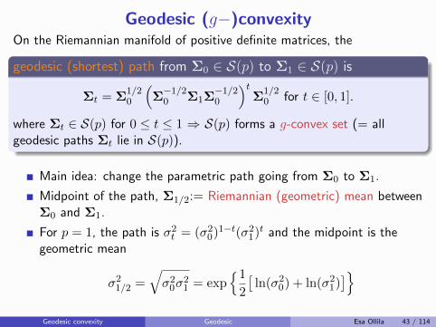
Geodesic (g−)convexityOn the Riemannian manifold of positive definite matrices, the
geodesic (shortest) path from Σ0 ∈ S(p) to Σ1 ∈ S(p) is
Σt = Σ1/20
(Σ−1/20 Σ1Σ
−1/20
)tΣ
1/20 for t ∈ [0, 1].
where Σt ∈ S(p) for 0 ≤ t ≤ 1 ⇒ S(p) forms a g-convex set (= allgeodesic paths Σt lie in S(p)).
Main idea: change the parametric path going from Σ0 to Σ1.
Midpoint of the path, Σ1/2:= Riemannian (geometric) mean betweenΣ0 and Σ1.
For p = 1, the path is σ2t = (σ20)1−t(σ21)t and the midpoint is thegeometric mean
σ21/2 =√σ20σ
21 = exp
{1
2
[ln(σ20) + ln(σ21)
]}
Geodesic convexity Geodesic Esa Ollila 43 / 114
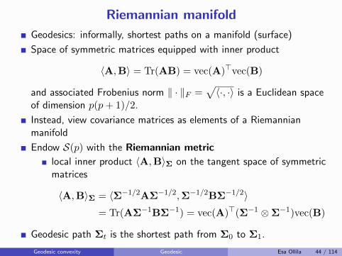
Riemannian manifold
Geodesics: informally, shortest paths on a manifold (surface)
Space of symmetric matrices equipped with inner product
〈A,B〉 = Tr(AB) = vec(A)>vec(B)
and associated Frobenius norm ‖ · ‖F =√〈·, ·〉 is a Euclidean space
of dimension p(p+ 1)/2.
Instead, view covariance matrices as elements of a Riemannianmanifold
Endow S(p) with the Riemannian metric
local inner product 〈A,B〉Σ on the tangent space of symmetricmatrices
〈A,B〉Σ = 〈Σ−1/2AΣ−1/2,Σ−1/2BΣ−1/2〉= Tr(AΣ−1BΣ−1) = vec(A)>(Σ−1 ⊗Σ−1)vec(B)
Geodesic path Σt is the shortest path from Σ0 to Σ1.
Geodesic convexity Geodesic Esa Ollila 44 / 114
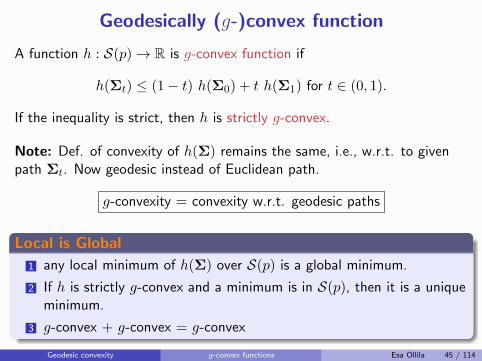
Geodesically (g-)convex function
A function h : S(p)→ R is g-convex function if
h(Σt) ≤ (1− t) h(Σ0) + t h(Σ1) for t ∈ (0, 1).
If the inequality is strict, then h is strictly g-convex.
Note: Def. of convexity of h(Σ) remains the same, i.e., w.r.t. to givenpath Σt. Now geodesic instead of Euclidean path.
g-convexity = convexity w.r.t. geodesic paths
Local is Global
1 any local minimum of h(Σ) over S(p) is a global minimum.
2 If h is strictly g-convex and a minimum is in S(p), then it is a uniqueminimum.
3 g-convex + g-convex = g-convex
Geodesic convexity g-convex functions Esa Ollila 45 / 114
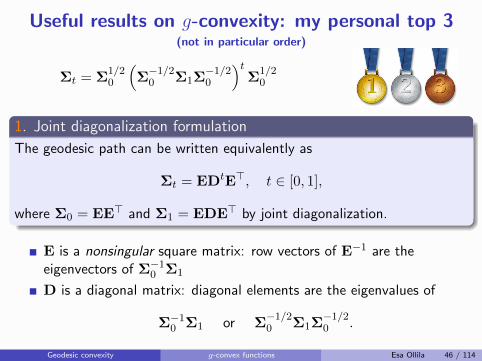
Useful results on g-convexity: my personal top 3(not in particular order)
Σt = Σ1/20
(Σ−1/20 Σ1Σ
−1/20
)tΣ
1/20
1. Joint diagonalization formulation
The geodesic path can be written equivalently as
Σt = EDtE>, t ∈ [0, 1],
where Σ0 = EE> and Σ1 = EDE> by joint diagonalization.
E is a nonsingular square matrix: row vectors of E−1 are theeigenvectors of Σ−10 Σ1
D is a diagonal matrix: diagonal elements are the eigenvalues of
Σ−10 Σ1 or Σ−1/20 Σ1Σ
−1/20 .
Geodesic convexity g-convex functions Esa Ollila 46 / 114
Useful results on g-convexity: my personal top 3
Σt = Σ1/20
(Σ−1/20 Σ1Σ
−1/20
)tΣ
1/20
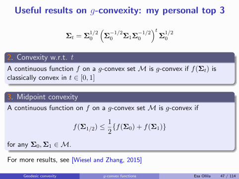
2. Convexity w.r.t. t
A continuous function f on a g-convex set M is g-convex if f(Σt) isclassically convex in t ∈ [0, 1]
3. Midpoint convexity
A continuous function on f on a g-convex set M is g-convex if
f(Σ1/2) ≤1
2{f(Σ0) + f(Σ1)}
for any Σ0,Σ1 ∈M.
For more results, see [Wiesel and Zhang, 2015]
Geodesic convexity g-convex functions Esa Ollila 47 / 114
Some geodesically (g-)convex functions
1 if h(Σ) is g-convex in Σ, then it is g-convex in Σ−1.
scalar case: if h(x) is convex in x = log(σ2) ∈ R, then it is convex in−x = log(σ−2) = − log(σ2).
2 ± log |Σ| is g-convex. (i.e., log-determinant is g-linear function)
scalar case: the scalar g-linear function is the logarithm.
3 a>Σ±1a is strictly g-convex (a 6= 0).
4 log |∑ni=1 HiΣ
±1Hi| is g-convex.
scalar case: log-sum-exp function is convex.
5 if f(Σ) is g-convex, then f(Σ1 ⊗Σ2) is jointly g-convex.
Geodesic convexity g-convex functions Esa Ollila 48 / 114
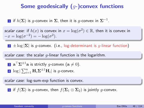
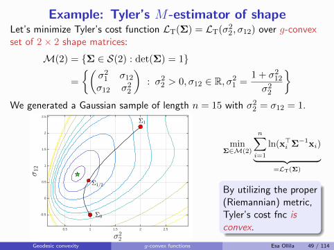
Example: Tyler’s M-estimator of shapeLet’s minimize Tyler’s cost function LT(Σ) = LT(σ22, σ12) over g-convexset of 2× 2 shape matrices:
M(2) = {Σ ∈ S(2) : det(Σ) = 1}
=
{(σ21 σ12σ12 σ22
): σ22 > 0, σ12 ∈ R, σ21 =
1 + σ212σ22
}
We generated a Gaussian sample of length n = 15 with σ22 = σ12 = 1.
<22
0.5 1 1.5 2 2.5
<12
-0.5
0
0.5
1
1.5
2
2.5
minΣ∈M(2)
n∑
i=1
ln(x>i Σ−1xi)
︸ ︷︷ ︸=LT(Σ)
Contours of LT(Σ)and the solution Σ.
Geodesic convexity g-convex functions Esa Ollila 49 / 114
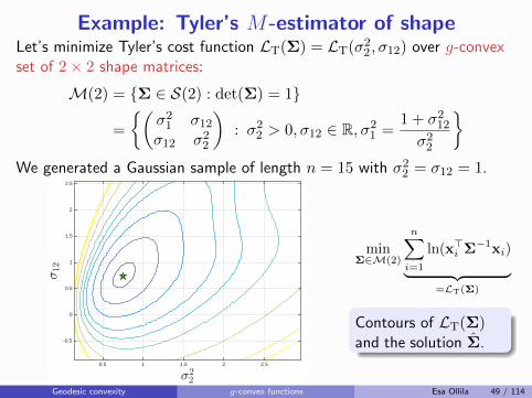
Example: Tyler’s M-estimator of shapeLet’s minimize Tyler’s cost function LT(Σ) = LT(σ22, σ12) over g-convexset of 2× 2 shape matrices:
M(2) = {Σ ∈ S(2) : det(Σ) = 1}
=
{(σ21 σ12σ12 σ22
): σ22 > 0, σ12 ∈ R, σ21 =
1 + σ212σ22
}
We generated a Gaussian sample of length n = 15 with σ22 = σ12 = 1.
'0
'1
<22
0.5 1 1.5 2 2.5
<12
-0.5
0
0.5
1
1.5
2
2.5
minΣ∈M(2)
n∑
i=1
ln(x>i Σ−1xi)
︸ ︷︷ ︸=LT(Σ)
Consider two pointsΣ0 and Σ1 of M.
Geodesic convexity g-convex functions Esa Ollila 49 / 114
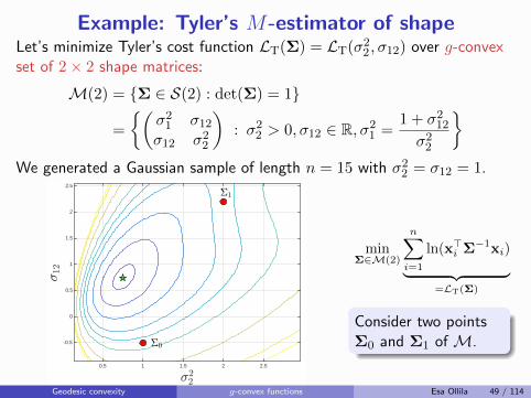
Example: Tyler’s M-estimator of shapeLet’s minimize Tyler’s cost function LT(Σ) = LT(σ22, σ12) over g-convexset of 2× 2 shape matrices:
M(2) = {Σ ∈ S(2) : det(Σ) = 1}
=
{(σ21 σ12σ12 σ22
): σ22 > 0, σ12 ∈ R, σ21 =
1 + σ212σ22
}
We generated a Gaussian sample of length n = 15 with σ22 = σ12 = 1.
'0
'1
'1=2
<22
0.5 1 1.5 2 2.5
<12
-0.5
0
0.5
1
1.5
2
2.5
minΣ∈M(2)
n∑
i=1
ln(x>i Σ−1xi)
︸ ︷︷ ︸=LT(Σ)
Their geodesic pathΣt and midpoint Σ1/2
Geodesic convexity g-convex functions Esa Ollila 49 / 114
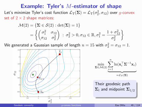
Example: Tyler’s M-estimator of shapeLet’s minimize Tyler’s cost function LT(Σ) = LT(σ22, σ12) over g-convexset of 2× 2 shape matrices:
M(2) = {Σ ∈ S(2) : det(Σ) = 1}
=
{(σ21 σ12σ12 σ22
): σ22 > 0, σ12 ∈ R, σ21 =
1 + σ212σ22
}
We generated a Gaussian sample of length n = 15 with σ22 = σ12 = 1.
'0
'1
'1=2
<22
0.5 1 1.5 2 2.5
<12
-0.5
0
0.5
1
1.5
2
2.5
minΣ∈M(2)
n∑
i=1
ln(x>i Σ−1xi)
︸ ︷︷ ︸=LT(Σ)
By utilizing the proper(Riemannian) metric,Tyler’s cost fnc isconvex.
Geodesic convexity g-convex functions Esa Ollila 49 / 114
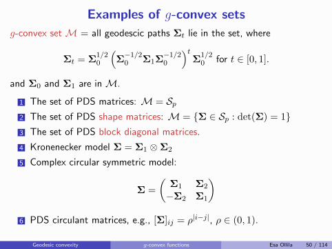
Examples of g-convex sets
g-convex set M = all geodescic paths Σt lie in the set, where
Σt = Σ1/20
(Σ−1/20 Σ1Σ
−1/20
)tΣ
1/20 for t ∈ [0, 1].
and Σ0 and Σ1 are in M.
1 The set of PDS matrices: M = Sp2 The set of PDS shape matrices: M = {Σ ∈ Sp : det(Σ) = 1}3 The set of PDS block diagonal matrices.
4 Kronenecker model Σ = Σ1 ⊗Σ2
5 Complex circular symmetric model:
Σ =
(Σ1 Σ2
−Σ2 Σ1
)
6 PDS circulant matrices, e.g., [Σ]ij = ρ|i−j|, ρ ∈ (0, 1).
Geodesic convexity g-convex functions Esa Ollila 50 / 114
I. Ad-hoc shrinkage SCM-s of multiple samples
II. ML- and M -estimators of scatter matrix
III. Geodesic convexity
IV. Regularized M -estimatorsShrinkage towards an identity matrixShrinkage towards a target matrix
V. Penalized estimation of multiple covariances
VI. Estimation of the regularization parameter
VII. Applications
References
Ollila, E. and Tyler, D. E. (2014).Regularized M -estimators of scatter matrix.IEEE Trans. Signal Process., 62(22):6059–6070.
Ollila, E., Soloveychik, I., Tyler, D. E. and Wiesel, A. (2016).Simultaneous penalized M-estimation of covariance matrices usinggeodesically convex optimizationJournal of Multivariate Analysis (under review), Cite as:arXiv:1608.08126 [stat.ME]http://arxiv.org/abs/1608.08126
Regularized M -estimators Esa Ollila 51 / 114
Honey, I shrunk the M-estimator of covariancematrix
⇒ The popular shrinkage SCM estimator (a.k.a Ledoit-Wolf estimator)is a member in the large class of regularized M -estimators of[Ollila and Tyler, 2014] that are presented in this section.
⇒ Our message: for non-Gaussian data or in the presence of outliers,you will do MUCH BETTER by shrinking a robust M -estimator ofcovariance!
Regularized M -estimators Esa Ollila 52 / 114
Regularized M-estimators of scatter matrix
Penalized cost function:
Lα(Σ) =1
n
n∑
i=1
ρ(x>i Σ−1xi)− ln |Σ−1|+ αP(Σ)
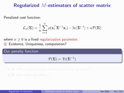
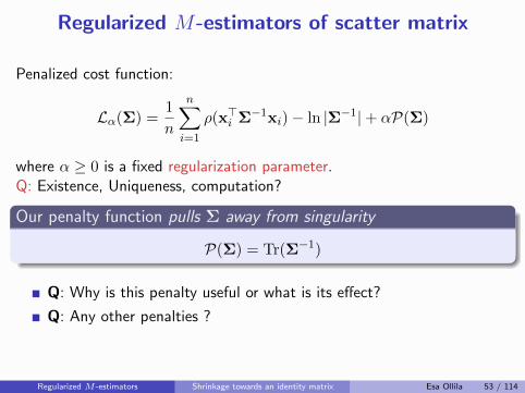
where α ≥ 0 is a fixed regularization parameter.Q: Existence, Uniqueness, computation?
Our penalty function
pulls Σ away from singularity
P(Σ) = Tr(Σ−1)
Q: Why is this penalty useful or what is its effect?
Q: Any other penalties ?
Regularized M -estimators Shrinkage towards an identity matrix Esa Ollila 53 / 114

Regularized M-estimators of scatter matrix
Penalized cost function:
Lα(Σ) =1
n
n∑
i=1
ρ(x>i Σ−1xi)− ln |Σ−1|+ αP(Σ)
where α ≥ 0 is a fixed regularization parameter.Q: Existence, Uniqueness, computation?
Our penalty function
pulls Σ away from singularity
P(Σ) = Tr(Σ−1)
Q: Why is this penalty useful or what is its effect?
Q: Any other penalties ?
Regularized M -estimators Shrinkage towards an identity matrix Esa Ollila 53 / 114
Regularized M-estimators of scatter matrix
Penalized cost function:
Lα(Σ) =1
n
n∑
i=1
ρ(x>i Σ−1xi)− ln |Σ−1|+ αP(Σ)
where α ≥ 0 is a fixed regularization parameter.Q: Existence, Uniqueness, computation?
Our penalty function pulls Σ away from singularity
P(Σ) = Tr(Σ−1)
Q: Why is this penalty useful or what is its effect?
Q: Any other penalties ?
Regularized M -estimators Shrinkage towards an identity matrix Esa Ollila 53 / 114
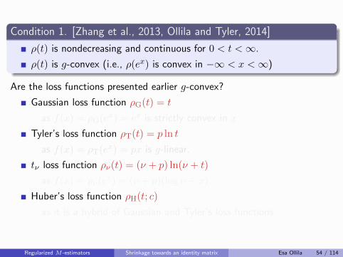
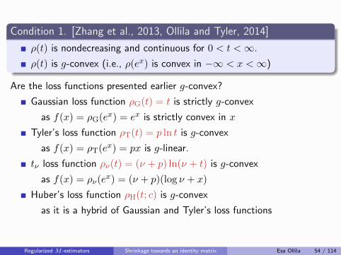
Condition 1. [Zhang et al., 2013, Ollila and Tyler, 2014]
ρ(t) is nondecreasing and continuous for 0 < t <∞.
ρ(t) is g-convex (i.e., ρ(ex) is convex in −∞ < x <∞)
Are the loss functions presented earlier g-convex?
Gaussian loss function ρG(t) = t
is strictly g-convex
as f(x) = ρG(ex) = ex is strictly convex in x
Tyler’s loss function ρT(t) = p ln t
is g-convex
as f(x) = ρT(ex) = px is g-linear.
tν loss function ρν(t) = (ν + p) ln(ν + t)
is g-convex
as f(x) = ρν(ex) = (ν + p)(log ν + x)
Huber’s loss function ρH(t; c)
is g-convex
as it is a hybrid of Gaussian and Tyler’s loss functions
Regularized M -estimators Shrinkage towards an identity matrix Esa Ollila 54 / 114
Condition 1. [Zhang et al., 2013, Ollila and Tyler, 2014]
ρ(t) is nondecreasing and continuous for 0 < t <∞.
ρ(t) is g-convex (i.e., ρ(ex) is convex in −∞ < x <∞)
Are the loss functions presented earlier g-convex?
Gaussian loss function ρG(t) = t is strictly g-convex
as f(x) = ρG(ex) = ex is strictly convex in x
Tyler’s loss function ρT(t) = p ln t
is g-convex
as f(x) = ρT(ex) = px is g-linear.
tν loss function ρν(t) = (ν + p) ln(ν + t)
is g-convex
as f(x) = ρν(ex) = (ν + p)(log ν + x)
Huber’s loss function ρH(t; c)
is g-convex
as it is a hybrid of Gaussian and Tyler’s loss functions
Regularized M -estimators Shrinkage towards an identity matrix Esa Ollila 54 / 114
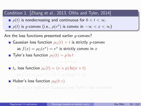
Condition 1. [Zhang et al., 2013, Ollila and Tyler, 2014]
ρ(t) is nondecreasing and continuous for 0 < t <∞.
ρ(t) is g-convex (i.e., ρ(ex) is convex in −∞ < x <∞)
Are the loss functions presented earlier g-convex?
Gaussian loss function ρG(t) = t is strictly g-convex
as f(x) = ρG(ex) = ex is strictly convex in x
Tyler’s loss function ρT(t) = p ln t is g-convex
as f(x) = ρT(ex) = px is g-linear.
tν loss function ρν(t) = (ν + p) ln(ν + t)
is g-convex
as f(x) = ρν(ex) = (ν + p)(log ν + x)
Huber’s loss function ρH(t; c)
is g-convex
as it is a hybrid of Gaussian and Tyler’s loss functions
Regularized M -estimators Shrinkage towards an identity matrix Esa Ollila 54 / 114
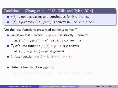
Condition 1. [Zhang et al., 2013, Ollila and Tyler, 2014]
ρ(t) is nondecreasing and continuous for 0 < t <∞.
ρ(t) is g-convex (i.e., ρ(ex) is convex in −∞ < x <∞)
Are the loss functions presented earlier g-convex?
Gaussian loss function ρG(t) = t is strictly g-convex
as f(x) = ρG(ex) = ex is strictly convex in x
Tyler’s loss function ρT(t) = p ln t is g-convex
as f(x) = ρT(ex) = px is g-linear.
tν loss function ρν(t) = (ν + p) ln(ν + t) is g-convex
as f(x) = ρν(ex) = (ν + p)(log ν + x)
Huber’s loss function ρH(t; c) is g-convex
as it is a hybrid of Gaussian and Tyler’s loss functions
Regularized M -estimators Shrinkage towards an identity matrix Esa Ollila 54 / 114
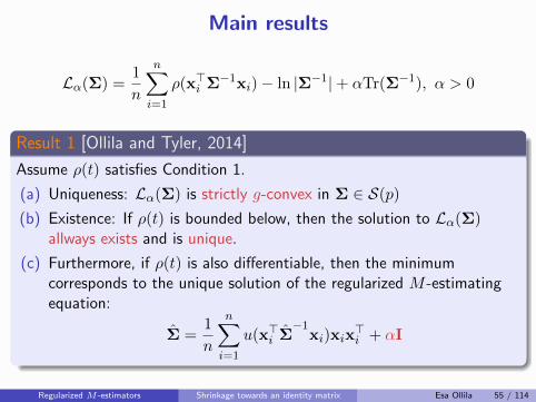
Main results
Lα(Σ) =1
n
n∑
i=1
ρ(x>i Σ−1xi)− ln |Σ−1|+ αTr(Σ−1), α > 0
Result 1 [Ollila and Tyler, 2014]
Assume ρ(t) satisfies Condition 1.
(a) Uniqueness: Lα(Σ) is strictly g-convex in Σ ∈ S(p)
(b) Existence: If ρ(t) is bounded below, then the solution to Lα(Σ)allways exists and is unique.
(c) Furthermore, if ρ(t) is also differentiable, then the minimumcorresponds to the unique solution of the regularized M -estimatingequation:
Σ =1
n
n∑
i=1
u(x>i Σ−1
xi)xix>i + αI
Regularized M -estimators Shrinkage towards an identity matrix Esa Ollila 55 / 114
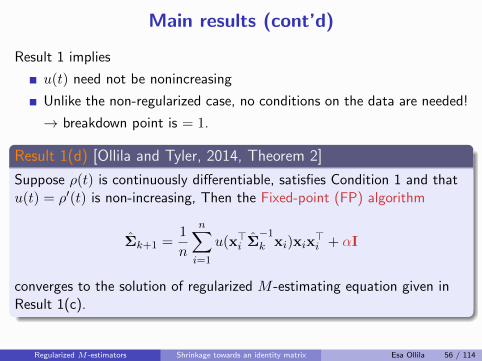
Main results (cont’d)
Result 1 implies
u(t) need not be nonincreasing
Unlike the non-regularized case, no conditions on the data are needed!
→ breakdown point is = 1.
Result 1(d) [Ollila and Tyler, 2014, Theorem 2]
Suppose ρ(t) is continuously differentiable, satisfies Condition 1 and thatu(t) = ρ′(t) is non-increasing, Then the Fixed-point (FP) algorithm
Σk+1 =1
n
n∑
i=1
u(x>i Σ−1k xi)xix
>i + αI
converges to the solution of regularized M -estimating equation given inResult 1(c).
Regularized M -estimators Shrinkage towards an identity matrix Esa Ollila 56 / 114
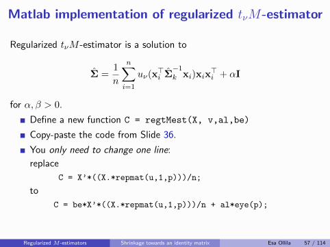
Matlab implementation of regularized tνM-estimator
Regularized tνM -estimator is a solution to
Σ =1
n
n∑
i=1
uν(x>i Σ−1k xi)xix
>i + αI
for α, β > 0.
Define a new function C = regtMest(X, v,al,be)
Copy-paste the code from Slide 36.
You only need to change one line:
replace
C = X’*((X.*repmat(u,1,p)))/n;
to
C = be*X’*((X.*repmat(u,1,p)))/n + al*eye(p);
Regularized M -estimators Shrinkage towards an identity matrix Esa Ollila 57 / 114
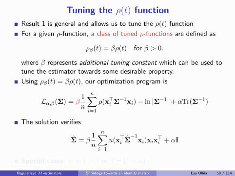
Tuning the ρ(t) function
Result 1 is general and allows us to tune the ρ(t) function
For a given ρ-function, a class of tuned ρ-functions are defined as
ρβ(t) = βρ(t) for β > 0.
where β represents additional tuning constant which can be used totune the estimator towards some desirable property.
Using ρβ(t) = βρ(t), our optimization program is
Lα,β(Σ) = β1
n
n∑
i=1
ρ(x>i Σ−1xi)− ln |Σ−1|+ αTr(Σ−1)
The solution verifies
Σ = β1
n
n∑
i=1
u(x>i Σ−1
xi)xix>i + αI
Special cases: α = 1− β or β = (1− α).
Regularized M -estimators Shrinkage towards an identity matrix Esa Ollila 58 / 114
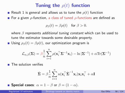
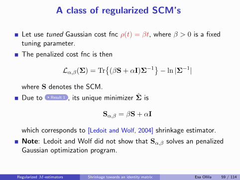
A class of regularized SCM’s
Let use tuned Gaussian cost fnc ρ(t) = βt, where β > 0 is a fixedtuning parameter.
The penalized cost fnc is then
Lα,β(Σ) = Tr{
(βS + αI)Σ−1}− ln |Σ−1|
where S denotes the SCM.
Due to Result 1 , its unique minimizer Σ is
Sα,β = βS + αI
which corresponds to [Ledoit and Wolf, 2004] shrinkage estimator.
Note: Ledoit and Wolf did not show that Sα,β solves an penalizedGaussian optimization program.
Regularized M -estimators Shrinkage towards an identity matrix Esa Ollila 59 / 114
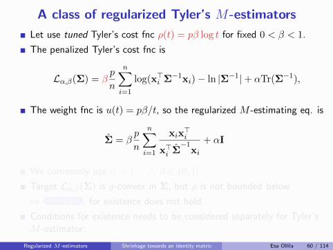
A class of regularized Tyler’s M-estimators
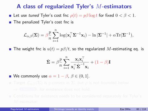
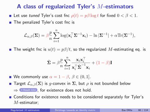
Let use tuned Tyler’s cost fnc ρ(t) = pβ log t for fixed 0 < β < 1.
The penalized Tyler’s cost fnc is
Lα,β(Σ) = βp
n
n∑
i=1
log(x>i Σ−1xi)− ln |Σ−1|+ αTr(Σ−1),
The weight fnc is u(t) = pβ/t, so the regularized M -estimating eq. is
Σ = βp
n
n∑
i=1
xix>i
x>i Σ−1
xi+ αI
We commonly use α = 1− β, β ∈ (0, 1].
Target Lα,β(Σ) is g-convex in Σ, but ρ is not bounded below
⇒ Result 1(b) , for existence does not hold.
Conditions for existence needs to be considered separately for Tyler’sM -estimator;
Regularized M -estimators Shrinkage towards an identity matrix Esa Ollila 60 / 114
A class of regularized Tyler’s M-estimators
Let use tuned Tyler’s cost fnc ρ(t) = pβ log t for fixed 0 < β < 1.
The penalized Tyler’s cost fnc is
Lα,β(Σ) = βp
n
n∑
i=1
log(x>i Σ−1xi)− ln |Σ−1|+ αTr(Σ−1),
The weight fnc is u(t) = pβ/t, so the regularized M -estimating eq. is
Σ = βp
n
n∑
i=1
xix>i
x>i Σ−1
xi+ (1− β)I
We commonly use α = 1− β, β ∈ (0, 1].
Target Lα,β(Σ) is g-convex in Σ, but ρ is not bounded below
⇒ Result 1(b) , for existence does not hold.
Conditions for existence needs to be considered separately for Tyler’sM -estimator;
Regularized M -estimators Shrinkage towards an identity matrix Esa Ollila 60 / 114
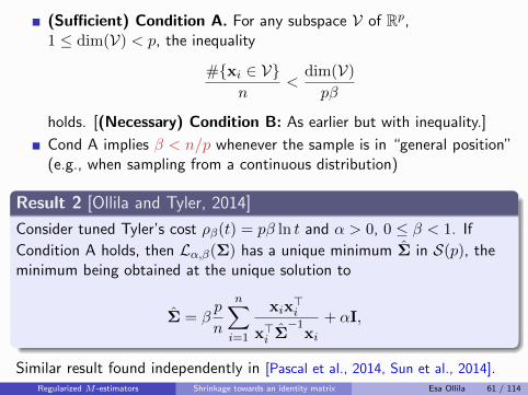
(Sufficient) Condition A. For any subspace V of Rp,1 ≤ dim(V) < p, the inequality
#{xi ∈ V}n
<dim(V)
pβ
holds. [(Necessary) Condition B: As earlier but with inequality.]
Cond A implies β < n/p whenever the sample is in “general position”(e.g., when sampling from a continuous distribution)
Result 2 [Ollila and Tyler, 2014]
Consider tuned Tyler’s cost ρβ(t) = pβ ln t and α > 0, 0 ≤ β < 1. If
Condition A holds, then Lα,β(Σ) has a unique minimum Σ in S(p), theminimum being obtained at the unique solution to
Σ = βp
n
n∑
i=1
xix>i
x>i Σ−1
xi+ αI,
Similar result found independently in [Pascal et al., 2014, Sun et al., 2014].Regularized M -estimators Shrinkage towards an identity matrix Esa Ollila 61 / 114
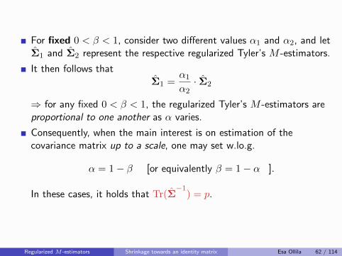
For fixed 0 < β < 1, consider two different values α1 and α2, and letΣ1 and Σ2 represent the respective regularized Tyler’s M -estimators.
It then follows thatΣ1 =
α1
α2· Σ2
⇒ for any fixed 0 < β < 1, the regularized Tyler’s M -estimators areproportional to one another as α varies.
Consequently, when the main interest is on estimation of thecovariance matrix up to a scale, one may set w.lo.g.
α = 1− β [or equivalently β = 1− α ].
In these cases, it holds that Tr(Σ−1
) = p.
Regularized M -estimators Shrinkage towards an identity matrix Esa Ollila 62 / 114
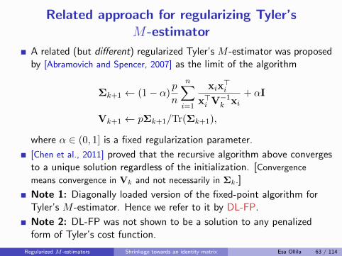
Related approach for regularizing Tyler’sM-estimator
A related (but different) regularized Tyler’s M -estimator was proposedby [Abramovich and Spencer, 2007] as the limit of the algorithm
Σk+1 ← (1− α)p
n
n∑
i=1
xix>i
x>i V−1k xi+ αI
Vk+1 ← pΣk+1/Tr(Σk+1),
where α ∈ (0, 1] is a fixed regularization parameter.
[Chen et al., 2011] proved that the recursive algorithm above convergesto a unique solution regardless of the initialization. [Convergence
means convergence in Vk and not necessarily in Σk.]
Note 1: Diagonally loaded version of the fixed-point algorithm forTyler’s M -estimator. Hence we refer to it by DL-FP.
Note 2: DL-FP was not shown to be a solution to any penalizedform of Tyler’s cost function.
Regularized M -estimators Shrinkage towards an identity matrix Esa Ollila 63 / 114
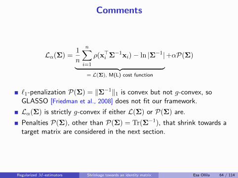
Comments
Lα(Σ) =1
n
n∑
i=1
ρ(x>i Σ−1xi)− ln |Σ−1|︸ ︷︷ ︸
= L(Σ), M(L) cost function
+αP(Σ)
`1-penalization P(Σ) = ‖Σ−1‖1 is convex but not g-convex, soGLASSO [Friedman et al., 2008] does not fit our framework.
Lα(Σ) is strictly g-convex if either L(Σ) or P(Σ) are.
Penalties P(Σ), other than P(Σ) = Tr(Σ−1), that shrink towards atarget matrix are considered in the next section.
Regularized M -estimators Shrinkage towards an identity matrix Esa Ollila 64 / 114
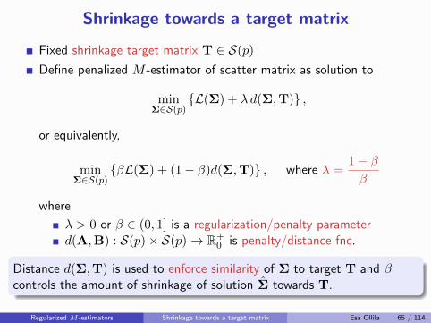
Shrinkage towards a target matrix
Fixed shrinkage target matrix T ∈ S(p)
Define penalized M -estimator of scatter matrix as solution to
minΣ∈S(p)
{L(Σ) + λ d(Σ,T)} ,
or equivalently,
minΣ∈S(p)
{βL(Σ) + (1− β)d(Σ,T)} , where λ =1− ββ
where
λ > 0 or β ∈ (0, 1] is a regularization/penalty parameterd(A,B) : S(p)× S(p)→ R+
0 is penalty/distance fnc.
Distance d(Σ,T) is used to enforce similarity of Σ to target T and βcontrols the amount of shrinkage of solution Σ towards T.
Regularized M -estimators Shrinkage towards a target matrix Esa Ollila 65 / 114
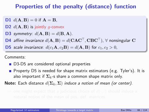
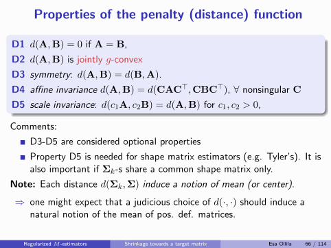
Properties of the penalty (distance) function
D1 d(A,B) = 0 if A = B,
D2 d(A,B) is jointly g-convex
D3 symmetry: d(A,B) = d(B,A).
D4 affine invariance d(A,B) = d(CAC>,CBC>), ∀ nonsingular C
D5 scale invariance: d(c1A, c2B) = d(A,B) for c1, c2 > 0,
Comments:
D3-D5 are considered optional properties
Property D5 is needed for shape matrix estimators (e.g. Tyler’s). It isalso important if Σk-s share a common shape matrix only.
Note: Each distance d(Σk,Σ) induce a notion of mean (or center).
⇒ one might expect that a judicious choice of d(·, ·) should induce anatural notion of the mean of pos. def. matrices.
Regularized M -estimators Shrinkage towards a target matrix Esa Ollila 66 / 114
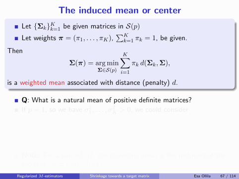
The induced mean or center
Let {Σk}Kk=1 be given matrices in S(p)
Let weights π = (π1, . . . , πK),∑K
k=1 πk = 1, be given.
Then
Σ(π) = arg minΣ∈S(p)
K∑
i=1
πk d(Σk,Σ),
is a weighted mean associated with distance (penalty) d.
Q: What is a natural mean of positive definite matrices?
If p = 1, so we have σ21, . . . , σ2K > 0, we could consider
• arithmetic mean σ2 = 1K
∑Kk=1 σ
2k.
• geometric mean σ2 =(σ21 · · ·σ2K
)1/K
• harmonic mean σ2 =(
1K
∑Kk=1(σ
2k)−1)−1
Note: For a pair σ20, σ21, the geometric mean is the midpoint of the
geodesic σ2t = (σ20)1−t(σ21)t.
Regularized M -estimators Shrinkage towards a target matrix Esa Ollila 67 / 114
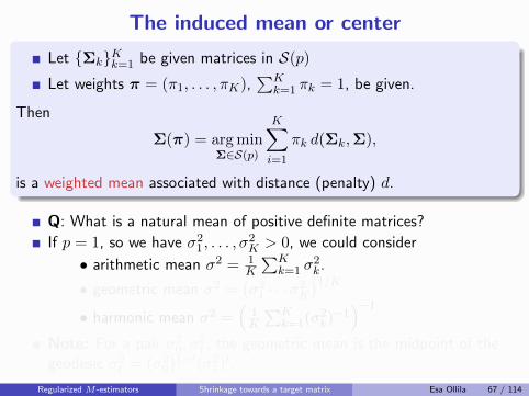
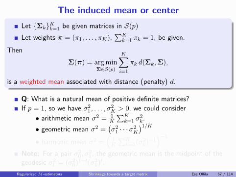
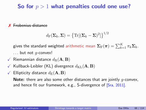
So for p > 1 what penalties could one use?
Frobenius distance
dF(Σk,Σ) ={
Tr[(Σk −Σ)2]}1/2
gives the standard weighted arithmetic mean ΣF(π) =∑K
k=1 πkΣk.
. . . but not g-convex!
X Riemannian distance dR(A,B)
X Kullback-Leibler (KL) divergence dKL(A,B)
X Ellipticity distance dE(A,B)
Note: there are also some other distances that are jointly g-convex,and hence fit our framework, e.g., S-divergence of [Sra, 2011].
Regularized M -estimators Shrinkage towards a target matrix Esa Ollila 68 / 114
So for p > 1 what penalties could one use?
7 Frobenius distance
dF(Σk,Σ) ={
Tr[(Σk −Σ)2]}1/2
gives the standard weighted arithmetic mean ΣF(π) =∑K
k=1 πkΣk.
. . . but not g-convex!
X Riemannian distance dR(A,B)
X Kullback-Leibler (KL) divergence dKL(A,B)
X Ellipticity distance dE(A,B)
Note: there are also some other distances that are jointly g-convex,and hence fit our framework, e.g., S-divergence of [Sra, 2011].
Regularized M -estimators Shrinkage towards a target matrix Esa Ollila 68 / 114
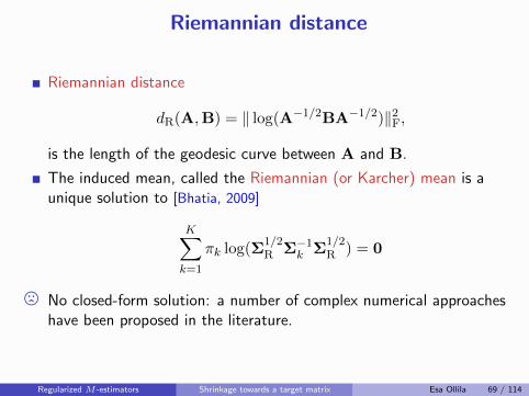
Riemannian distance
Riemannian distance
dR(A,B) = ‖ log(A−1/2BA−1/2)‖2F,
is the length of the geodesic curve between A and B.
The induced mean, called the Riemannian (or Karcher) mean is aunique solution to [Bhatia, 2009]
K∑
k=1
πk log(Σ1/2R Σ−1k Σ
1/2R ) = 0
/ No closed-form solution: a number of complex numerical approacheshave been proposed in the literature.
Regularized M -estimators Shrinkage towards a target matrix Esa Ollila 69 / 114
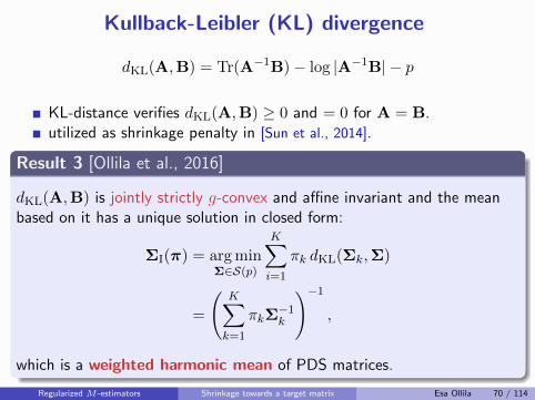
Kullback-Leibler (KL) divergence
dKL(A,B) = Tr(A−1B)− log |A−1B| − p
KL-distance verifies dKL(A,B) ≥ 0 and = 0 for A = B.utilized as shrinkage penalty in [Sun et al., 2014].
Result 3 [Ollila et al., 2016]
dKL(A,B) is jointly strictly g-convex and affine invariant and the meanbased on it has a unique solution in closed form:
ΣI(π) = arg minΣ∈S(p)
K∑
i=1
πk dKL(Σk,Σ)
=
(K∑
k=1
πkΣ−1k
)−1,
which is a weighted harmonic mean of PDS matrices.
Regularized M -estimators Shrinkage towards a target matrix Esa Ollila 70 / 114
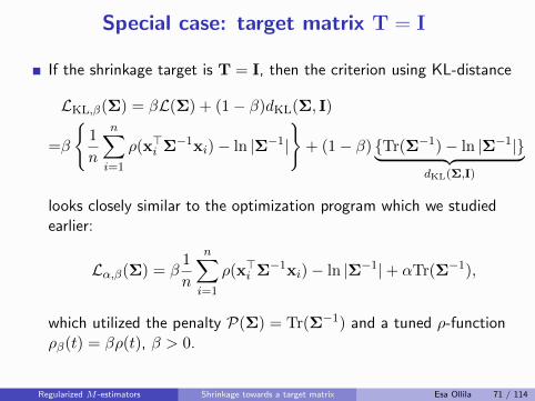
Special case: target matrix T = I
If the shrinkage target is T = I, then the criterion using KL-distance
LKL,β(Σ) = βL(Σ) + (1− β)dKL(Σ, I)
=β
{1
n
n∑
i=1
ρ(x>i Σ−1xi)− ln |Σ−1|}
+ (1− β) {Tr(Σ−1)− ln |Σ−1|}︸ ︷︷ ︸dKL(Σ,I)
looks closely similar to the optimization program which we studiedearlier:
Lα,β(Σ) = β1
n
n∑
i=1
ρ(x>i Σ−1xi)− ln |Σ−1|+ αTr(Σ−1),
which utilized the penalty P(Σ) = Tr(Σ−1) and a tuned ρ-functionρβ(t) = βρ(t), β > 0.
Regularized M -estimators Shrinkage towards a target matrix Esa Ollila 71 / 114
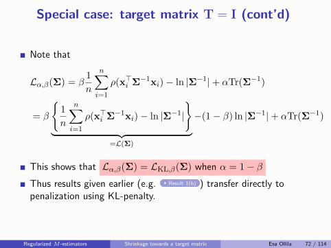
Special case: target matrix T = I (cont’d)
Note that
Lα,β(Σ) = β1
n
n∑
i=1
ρ(x>i Σ−1xi)− ln |Σ−1|+ αTr(Σ−1)
= β
{1
n
n∑
i=1
ρ(x>i Σ−1xi)− ln |Σ−1|}
︸ ︷︷ ︸=L(Σ)
−(1− β) ln |Σ−1|+ αTr(Σ−1)
This shows that Lα,β(Σ) = LKL,β(Σ) when α = 1− βThus results given earlier (e.g. Result 1(b) ) transfer directly topenalization using KL-penalty.
Regularized M -estimators Shrinkage towards a target matrix Esa Ollila 72 / 114
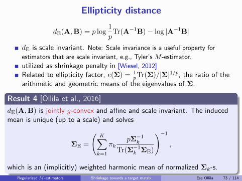
Ellipticity distance
dE(A,B) = p log1
pTr(A−1B)− log |A−1B|
dE is scale invariant. Note: Scale invariance is a useful property for
estimators that are scale invariant, e.g., Tyler’s M -estimator.
utilized as shrinkage penalty in [Wiesel, 2012]
Related to ellipticity factor, e(Σ) = 1pTr(Σ)/|Σ|1/p, the ratio of the
arithmetic and geometric means of the eigenvalues of Σ.
Result 4 [Ollila et al., 2016]
dE(A,B) is jointly g-convex and affine and scale invariant. The inducedmean is unique (up to a scale) and solves
ΣE =
(K∑
k=1
πkpΣ−1k
Tr(Σ−1k ΣE)
)−1,
which is an (implicitly) weighted harmonic mean of normalized Σk-s.
Regularized M -estimators Shrinkage towards a target matrix Esa Ollila 73 / 114
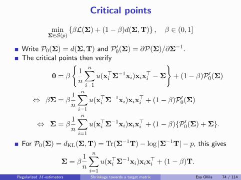
Critical points
minΣ∈S(p)
{βL(Σ) + (1− β)d(Σ,T)} , β ∈ (0, 1]
Write P0(Σ) = d(Σ,T) and P ′0(Σ) = ∂P(Σ)/∂Σ−1.The critical points then verify
0 = β
{1
n
n∑
i=1
u(x>i Σ−1xi)xix>i −Σ
}+ (1− β)P ′0(Σ)
⇔ βΣ = β1
n
n∑
i=1
u(x>i Σ−1xi)xix>i + (1− β)P ′0(Σ)
⇔ Σ = β1
n
n∑
i=1
u(x>i Σ−1xi)xix>i + (1− β){P ′0(Σ) + Σ}.
For P0(Σ) = dKL(Σ,T) = Tr(Σ−1T)− log |Σ−1T| − p, this gives
Σ = β1
n
n∑
i=1
u(x>i Σ−1xi)xix>i + (1− β)T.
Regularized M -estimators Shrinkage towards a target matrix Esa Ollila 74 / 114
I. Ad-hoc shrinkage SCM-s of multiple samples
II. ML- and M -estimators of scatter matrix
III. Geodesic convexity
IV. Regularized M -estimators
V. Penalized estimation of multiple covariances
VI. Estimation of the regularization parameter
VII. Applications
Reference
Ollila, E., Soloveychik, I., Tyler, D. E. and Wiesel, A. (2016).Simultaneous penalized M-estimation of covariance matrices usinggeodesically convex optimizationJournal of Multivariate Analysis (under review), Cite as:arXiv:1608.08126 [stat.ME]http://arxiv.org/abs/1608.08126
Penalized estimation of multiple covariances Esa Ollila 75 / 114
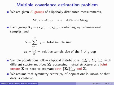
Multiple covariance estimation problem
We are given K groups of elliptically distributed measurements,
x11, . . . ,x1n1 , . . . , xK1, . . . ,xKnK
Each group Xk = {xk1, . . . ,xknk} containing nk p-dimensional
samples, and
N =
K∑
i=1
nk = total sample size
πk =nkN
= relative sample size of the k-th group
Sample populations follow elliptical distributions, Ep(µk,Σk, gk), withdifferent scatter matrices Σk possessing mutual structure or a jointcenter Σ ⇒ need to estimate both {Σk}Kk=1 and Σ.
We assume that symmetry center µk of populations is known or thatdata is centered.
Penalized estimation of multiple covariances Esa Ollila 76 / 114
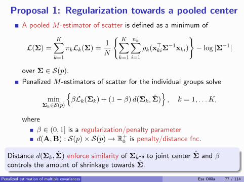
Proposal 1: Regularization towards a pooled center
A pooled M -estimator of scatter is defined as a minimum of
L(Σ) =
K∑
k=1
πkLk(Σ) =1
N
{K∑
k=1
nk∑
i=1
ρk(x>kiΣ
−1xki)
}− log |Σ−1|
over Σ ∈ S(p).
Penalized M -estimators of scatter for the individual groups solve
minΣk∈S(p)
{βLk(Σk) + (1− β) d(Σk, Σ)
}, k = 1, . . .K,
where
β ∈ (0, 1] is a regularization/penalty parameterd(A,B) : S(p)× S(p)→ R+
0 is penalty/distance fnc.
Distance d(Σk, Σ) enforce similarity of Σk-s to joint center Σ and βcontrols the amount of shrinkage towards Σ.
Penalized estimation of multiple covariances Esa Ollila 77 / 114
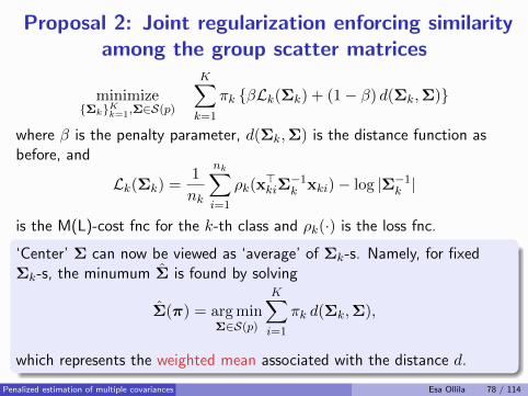
Proposal 2: Joint regularization enforcing similarityamong the group scatter matrices
minimize{Σk}Kk=1,Σ∈S(p)
K∑
k=1
πk {βLk(Σk) + (1− β) d(Σk,Σ)}
where β is the penalty parameter, d(Σk,Σ) is the distance function asbefore, and
Lk(Σk) =1
nk
nk∑
i=1
ρk(x>kiΣ
−1k xki)− log |Σ−1k |
is the M(L)-cost fnc for the k-th class and ρk(·) is the loss fnc.
‘Center’ Σ can now be viewed as ‘average’ of Σk-s. Namely, for fixedΣk-s, the minumum Σ is found by solving
Σ(π) = arg minΣ∈S(p)
K∑
i=1
πk d(Σk,Σ),
which represents the weighted mean associated with the distance d.
Penalized estimation of multiple covariances Esa Ollila 78 / 114
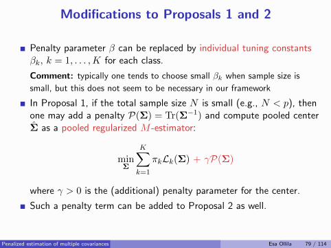
Modifications to Proposals 1 and 2
Penalty parameter β can be replaced by individual tuning constantsβk, k = 1, . . . ,K for each class.
Comment: typically one tends to choose small βk when sample size is
small, but this does not seem to be necessary in our framework
In Proposal 1, if the total sample size N is small (e.g., N < p), thenone may add a penalty P(Σ) = Tr(Σ−1) and compute pooled centerΣ as a pooled regularized M -estimator:
minΣ
K∑
k=1
πkLk(Σ) + γP(Σ)
where γ > 0 is the (additional) penalty parameter for the center.
Such a penalty term can be added to Proposal 2 as well.
Penalized estimation of multiple covariances Esa Ollila 79 / 114
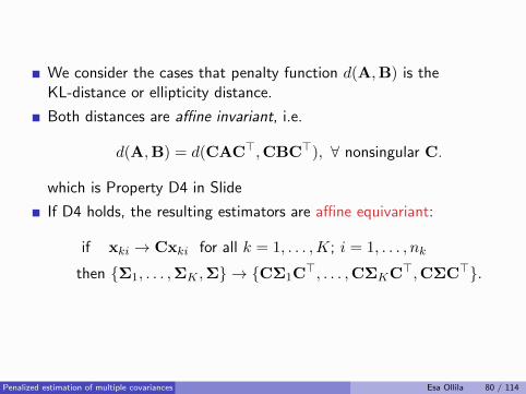
We consider the cases that penalty function d(A,B) is theKL-distance or ellipticity distance.
Both distances are affine invariant, i.e.
d(A,B) = d(CAC>,CBC>), ∀ nonsingular C.
which is Property D4 in Slide
If D4 holds, the resulting estimators are affine equivariant:
if xki → Cxki for all k = 1, . . . ,K; i = 1, . . . , nk
then {Σ1, . . . ,ΣK ,Σ} → {CΣ1C>, . . . ,CΣKC>,CΣC>}.
Penalized estimation of multiple covariances Esa Ollila 80 / 114
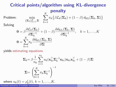
Critical points/algorithm using KL-divergencepenalty
Problem: min{Σk}Kk=1,Σ
K∑
k=1
πk{βLk(Σk) + (1− β) dKL(Σk,Σ)
}
Solving
0 = β∂Lk(Σk)
∂Σ−1k+ (1− β)
∂dKL(Σk,Σ)
∂Σ−1k, k = 1, . . . ,K
0 =
K∑
k=1
πk∂dKL(Σk,Σ)
∂Σ
yields estimating equations
Σk= β1
nk
nk∑
i=1
uk(x>kiΣ
−1k xki)xkix
>ki + (1− β)Σ
Σ=
(K∑
k=1
πkΣ−1k
)−1
where uk(t) = ρ′k(t), k = 1, . . . ,K.Penalized estimation of multiple covariances Esa Ollila 81 / 114
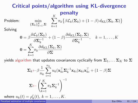
Critical points/algorithm using KL-divergencepenalty
Problem: min{Σk}Kk=1,Σ
K∑
k=1
πk{βLk(Σk) + (1− β) dKL(Σk,Σ)
}
Solving
0 = β∂Lk(Σk)
∂Σ−1k+ (1− β)
∂dKL(Σk,Σ)
∂Σ−1k, k = 1, . . . ,K
0 =
K∑
k=1
πk∂dKL(Σk,Σ)
∂Σ
yields algorithm that updates covariances cyclically from Σ1, . . .ΣK to Σ
Σk←β1
nk
nk∑
i=1
uk(x>kiΣ
−1k xki)xkix
>ki + (1− β)Σ
Σ←(
K∑
k=1
πkΣ−1k
)−1
where uk(t) = ρ′k(t), k = 1, . . . ,K.Penalized estimation of multiple covariances Esa Ollila 81 / 114
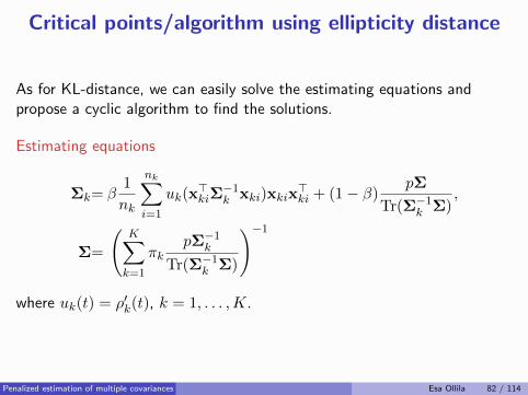
Critical points/algorithm using ellipticity distance
As for KL-distance, we can easily solve the estimating equations andpropose a cyclic algorithm to find the solutions.
Estimating equations
Σk= β1
nk
nk∑
i=1
uk(x>kiΣ
−1k xki)xkix
>ki + (1− β)
pΣ
Tr(Σ−1k Σ),
Σ=
(K∑
k=1
πkpΣ−1k
Tr(Σ−1k Σ)
)−1
where uk(t) = ρ′k(t), k = 1, . . . ,K.
Penalized estimation of multiple covariances Esa Ollila 82 / 114
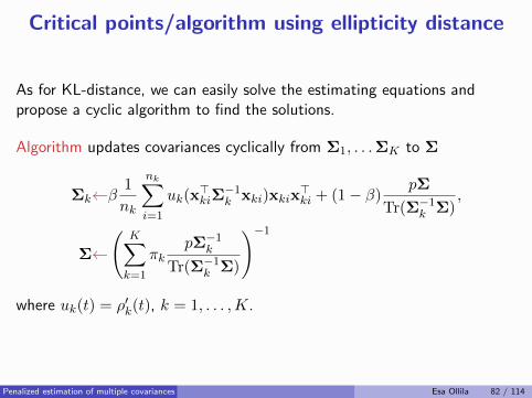
Critical points/algorithm using ellipticity distance
As for KL-distance, we can easily solve the estimating equations andpropose a cyclic algorithm to find the solutions.
Algorithm updates covariances cyclically from Σ1, . . .ΣK to Σ
Σk←β1
nk
nk∑
i=1
uk(x>kiΣ
−1k xki)xkix
>ki + (1− β)
pΣ
Tr(Σ−1k Σ),
Σ←(
K∑
k=1
πkpΣ−1k
Tr(Σ−1k Σ)
)−1
where uk(t) = ρ′k(t), k = 1, . . . ,K.
Penalized estimation of multiple covariances Esa Ollila 82 / 114
I. Ad-hoc shrinkage SCM-s of multiple samples
II. ML- and M -estimators of scatter matrix
III. Geodesic convexity
IV. Regularized M -estimators
V. Penalized estimation of multiple covariances
VI. Estimation of the regularization parameterCross-validationOracle approach
VII. Applications
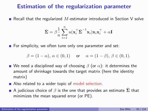
Estimation of the regularization parameter
Recall that the regularized M -estimator introduced in Section V solve
Σ = β1
n
n∑
i=1
u(x>i Σ−1
xi)xix>i + αI
For simplicity, we often tune only one parameter and set:
β = (1− α), α ∈ (0, 1) or α = (1− β), β ∈ (0, 1).
We need a disciplined way of choosing β (or α): it determines theamount of shrinkage towards the target matrix (here the identitymatrix)
Also related to a wider topic of model selection.
A judicious choice of β is the one that provides an estimate Σ thatminimizes the mean squared error (or PE).
Estimation of the regularization parameter Esa Ollila 83 / 114
Approaches:
1 Cross-validation
2 Oracle/Clairvoyant approach
3 Expected likelihood approach[Abramovich and Besson, 2013, Besson and Abramovich, 2013]
4 Random matrix theory (Frederic’s talk).
Only the first two topics are addressed in this tutorial.
Estimation of the regularization parameter Esa Ollila 84 / 114
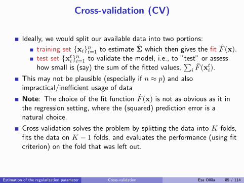
Cross-validation (CV)
Ideally, we would split our available data into two portions:
training set {xi}ni=1 to estimate Σ which then gives the fit F (x).test set {xti}ni=1 to validate the model, i.e., to ”test” or assesshow small is (say) the sum of the fitted values,
∑i F (xti).
This may not be plausible (especially if n ≈ p) and alsoimpractical/inefficient usage of data
Note: The choice of the fit function F (x) is not as obvious as it inthe regression setting, where the (squared) prediction error is anatural choice.
Cross validation solves the problem by splitting the data into K folds,fits the data on K − 1 folds, and evaluates the performance (using fitcriterion) on the fold that was left out.
Estimation of the regularization parameter Cross-validation Esa Ollila 85 / 114
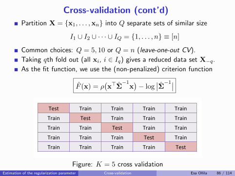
Cross-validation (cont’d)
Partition X = {x1, . . . ,xn} into Q separate sets of similar size
I1 ∪ I2 ∪ · · · ∪ IQ = {1, . . . , n} ≡ [n]
Common choices: Q = 5, 10 or Q = n (leave-one-out CV).
Taking qth fold out (all xi, i ∈ Iq) gives a reduced data set X−q.
As the fit function, we use the (non-penalized) criterion function
F (x) = ρ(x>Σ
−1x)− log
∣∣Σ−1∣∣
Test Train Train Train Train
Train Test Train Train Train
Train Train Test Train Train
Train Train Train Test Train
Train Train Train Train Test
Figure: K = 5 cross validationEstimation of the regularization parameter Cross-validation Esa Ollila 86 / 114
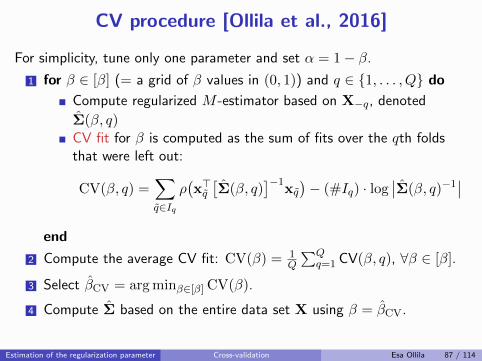
CV procedure [Ollila et al., 2016]
For simplicity, tune only one parameter and set α = 1− β.
1 for β ∈ [β] (= a grid of β values in (0, 1)) and q ∈ {1, . . . , Q} do
Compute regularized M -estimator based on X−q, denoted
Σ(β, q)CV fit for β is computed as the sum of fits over the qth foldsthat were left out:
CV(β, q) =∑
q∈Iq
ρ(x>q[Σ(β, q)
]−1xq)− (#Iq) · log
∣∣Σ(β, q)−1∣∣
end
2 Compute the average CV fit: CV(β) = 1Q
∑Qq=1 CV(β, q), ∀β ∈ [β].
3 Select βCV = arg minβ∈[β] CV(β).
4 Compute Σ based on the entire data set X using β = βCV.
Estimation of the regularization parameter Cross-validation Esa Ollila 87 / 114
Oracle/Clairvoyant approach
The regularized M -estimator of scatter is a solution of
Σ = β1
n
n∑
i=1
u(x>i Σ−1
xi)xix>i + αI
for given penalty parameters α, β > 0.
Since Σ does not have a closed form expression, deriving an analyticexpression for an expected loss (such as the MSE) is virtuallyimpossible.
Solution: use an approximation for Σ.
Given the true scatter (covariance) matrix Σ0, then
Σα,β = (1− α)1
n
n∑
i=1
u(x>i Σ−10 xi)xix>i + αI
called the clairvoyant estimator, is a closed-form approximation of Σ.
Estimation of the regularization parameter Oracle approach Esa Ollila 88 / 114
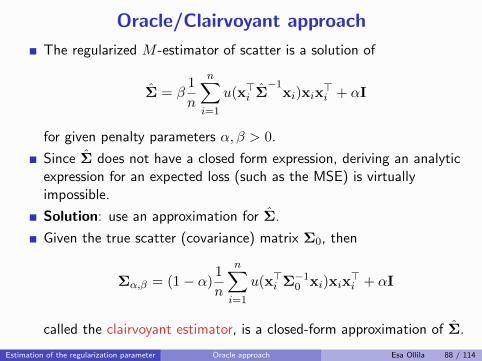
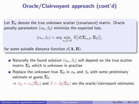
Oracle/Clairvoyant approach (cont’d)
Let Σ0 denote the true unknown scatter (covariance) matrix. Oraclepenalty parameters (α0, β0) minimize the expected loss,
(αo, βo) = arg minα,β>0
E[d(Σα,β,Σ0)
],
for some suitable distance function d(A,B).
Naturally the found solution (αo, βo) will depend on the true scattermatrix Σ0 which is unknown in practise.
Replace the unknown true Σ0 in α0 and β0 with some preliminaryestimate or guess Σ0
⇒ αo = αo(Σ0) and β = β0(Σ0) are the oracle/clairvoyant estimates.
Estimation of the regularization parameter Oracle approach Esa Ollila 89 / 114
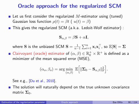
Oracle approach for the regularized SCM
Let us first consider the regularized M -estimator using (tuned)Gaussian loss function ρ(t) = βt ( u(t) = β)
This gives the regularized SCM (a.k.a. Ledoit-Wolf estimator) :
Sα,β = βS + αI,
where S is the unbiased SCM S = 1n−1
∑ni=1 xix
>i , so E[S] = Σ
Clairvoyant (oracle) estimator of (α, β) ∈ R+0 × R+ is defined as a
minimizer of the mean squared error (MSE),
(αo, βo) = arg min(α,β)
E[‖Σ0 − Sα,β‖2F
].
See e.g., [Du et al., 2010].
The solution will naturally depend on the true unknown covariancematrix Σ0.
Estimation of the regularization parameter Oracle approach Esa Ollila 90 / 114
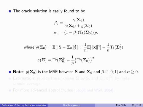
The oracle solution is easily found to be
βo =γ(Σ0)
γ(Σ0) + %(Σ0)
αo = (1− β0)Tr(Σ0)/p.
where %(Σ0) = E[‖S−Σ0‖2F] =1
nE[‖x‖4]− 1
nTr(Σ2
0)
γ(Σ) = Tr(Σ20)−
1
p
{Tr(Σ0)
}2
Note: %(Σ0) is the MSE between S and Σ0 and β ∈ [0, 1] and α ≥ 0.
Estimation: replace the unknown Σ by S, and E[‖x‖4] by finitesample average.
For more advanced approach, see [Ledoit and Wolf, 2004].
Estimation of the regularization parameter Oracle approach Esa Ollila 91 / 114
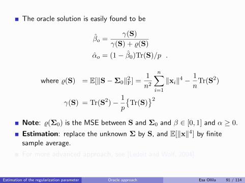
The oracle solution is easily found to be
βo =γ(S)
γ(S) + %(S)
αo = (1− β0)Tr(S)/p .
where %(S) = E[‖S−Σ0‖2F] =1
n2
n∑
i=1
‖xi‖4 −1
nTr(S2)
γ(S) = Tr(S2)− 1
p
{Tr(S)
}2
Note: %(Σ0) is the MSE between S and Σ0 and β ∈ [0, 1] and α ≥ 0.
Estimation: replace the unknown Σ by S, and E[‖x‖4] by finitesample average.
For more advanced approach, see [Ledoit and Wolf, 2004].
Estimation of the regularization parameter Oracle approach Esa Ollila 91 / 114
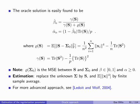
The oracle solution is easily found to be
βo =γ(S)
γ(S) + %(S)
αo = (1− β0)Tr(S)/p .
where %(S) = E[‖S−Σ0‖2F] =1
n2
n∑
i=1
‖xi‖4 −1
nTr(S2)
γ(S) = Tr(S2)− 1
p
{Tr(S)
}2
Note: %(Σ0) is the MSE between S and Σ0 and β ∈ [0, 1] and α ≥ 0.
Estimation: replace the unknown Σ by S, and E[‖x‖4] by finitesample average.
For more advanced approach, see [Ledoit and Wolf, 2004].
Estimation of the regularization parameter Oracle approach Esa Ollila 91 / 114
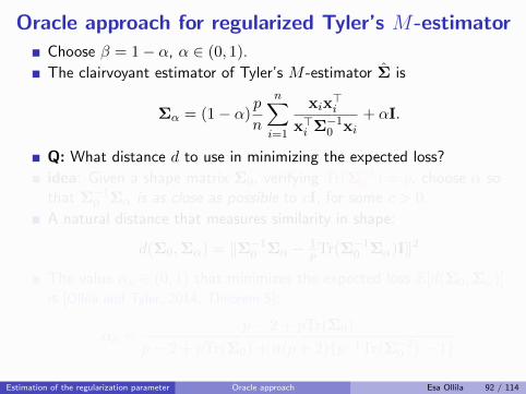
Oracle approach for regularized Tyler’s M-estimator
Choose β = 1− α, α ∈ (0, 1).
The clairvoyant estimator of Tyler’s M -estimator Σ is
Σα = (1− α)p
n
n∑
i=1
xix>i
x>i Σ−10 xi+ αI.
Q: What distance d to use in minimizing the expected loss?
idea: Given a shape matrix Σ0, verifying Tr(Σ−10 ) = p, choose α sothat Σ−10 Σα is as close as possible to cI, for some c > 0.
A natural distance that measures similarity in shape:
d(Σ0,Σα) = ‖Σ−10 Σα − 1pTr(Σ−10 Σα)I‖2
The value αo ∈ (0, 1) that minimizes the expected loss E[d(Σ0,Σα)]is [Ollila and Tyler, 2014, Theorem 5]:
αo =p− 2 + pTr(Σ0)
p− 2 + pTr(Σ0) + n(p+ 2){p−1Tr(Σ−20 )− 1}
Estimation of the regularization parameter Oracle approach Esa Ollila 92 / 114
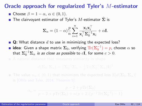
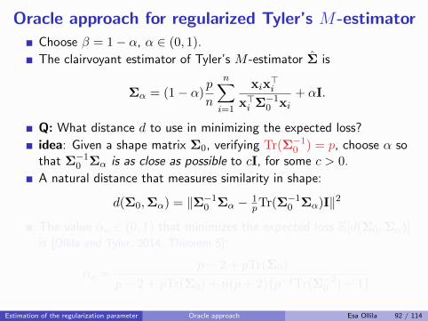
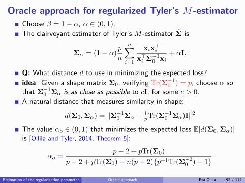

Oracle approach for regularized Tyler’s M-estimator
Similar expression is derived for complex-valued case also in[Ollila and Tyler, 2014].
Estimate αo = αo(Σ0) is obtained by using an estimate Σ0 which is
• Conventional (non-regularized) Tyler’s M -estimator normalized
so that Tr(Σ−10 ) = p when n ≥ p
• Regularized Tyler’s M -estimator using β < n/p and α = 1− βwhen n < p.
Estimation of the regularization parameter Oracle approach Esa Ollila 93 / 114
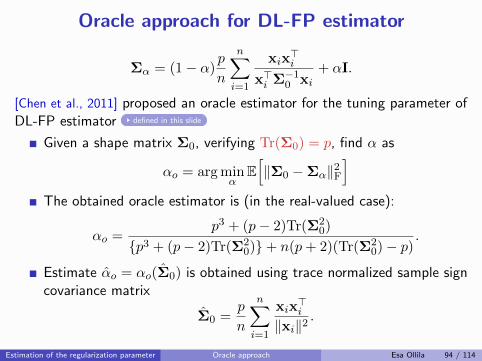
Oracle approach for DL-FP estimator
Σα = (1− α)p
n
n∑
i=1
xix>i
x>i Σ−10 xi+ αI.
[Chen et al., 2011] proposed an oracle estimator for the tuning parameter ofDL-FP estimator defined in this slide
Given a shape matrix Σ0, verifying Tr(Σ0) = p, find α as
αo = arg minα
E[‖Σ0 −Σα‖2F
]
The obtained oracle estimator is (in the real-valued case):
αo =p3 + (p− 2)Tr(Σ2
0)
{p3 + (p− 2)Tr(Σ20)}+ n(p+ 2)(Tr(Σ2
0)− p).
Estimate αo = αo(Σ0) is obtained using trace normalized sample signcovariance matrix
Σ0 =p
n
n∑
i=1
xix>i
‖xi‖2.
Estimation of the regularization parameter Oracle approach Esa Ollila 94 / 114
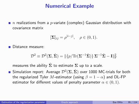
Numerical Example
n realizations from a p-variate (complex) Gaussian distribution withcovariance matrix
[Σ]ij = ρ|i−j|, ρ ∈ (0, 1).
Distance measure:
D2 ≡ D2(Σ, Σ) = ‖{p/Tr(Σ−1Σ)}Σ−1Σ− I‖2F
measures the ability Σ to estimate Σ up to a scale.
Simulation report: Average D2(Σ, Σ) over 1000 MC-trials for boththe regularized Tyler M -estimator (using β = 1− α) and DL-FPestimator for different values of penalty parameter α ∈ (0, 1).
Estimation of the regularization parameter Oracle approach Esa Ollila 95 / 114
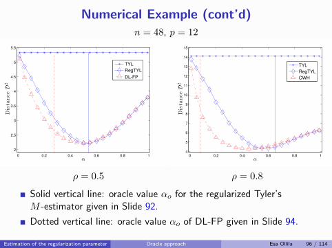
Numerical Example (cont’d)n = 48, p = 12
0 0.2 0.4 0.6 0.8 1
2
2.5
3
3.5
4
4.5
5
5.5
α
DistanceD
2
TYL
RegTYL
DL-FP
0 0.2 0.4 0.6 0.8 14
5
6
7
8
9
10
11
12
13
14
15
α
DistanceD
2
TYL
RegTYL
CWH
ρ = 0.5 ρ = 0.8
Solid vertical line: oracle value αo for the regularized Tyler’sM -estimator given in Slide 92.
Dotted vertical line: oracle value αo of DL-FP given in Slide 94.
Estimation of the regularization parameter Oracle approach Esa Ollila 96 / 114
I. Ad-hoc shrinkage SCM-s of multiple samples
II. ML- and M -estimators of scatter matrix
III. Geodesic convexity
IV. Regularized M -estimators
V. Penalized estimation of multiple covariances
VI. Estimation of the regularization parameter
VII. ApplicationsRegularized discriminant analysisMatched filter detection
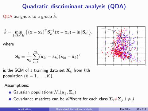
Quadratic discriminant analysis (QDA)
QDA assigns x to a group k:
k = min1≤k≤K
{(x− xk)
>S−1k (x− xk) + ln |Sk|}.
where
Sk =1
nk
nk∑
i=1
(xki − xk)(xki − xk)>
is the SCM of a training data set Xk from kthpopulation (k = 1, . . . ,K).
Assumptions:
Gaussian populations Np(µk,Σk)
Covariance matrices can be different for each class Σi 6=Σj i 6= j
Applications Regularized discriminant analysis Esa Ollila 97 / 114
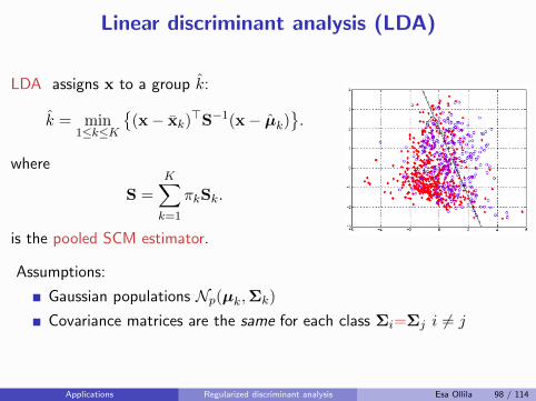
Linear discriminant analysis (LDA)
LDA assigns x to a group k:
k = min1≤k≤K
{(x− xk)
>S−1(x− µk)}.
where
S =
K∑
k=1
πkSk.
is the pooled SCM estimator.
Assumptions:
Gaussian populations Np(µk,Σk)
Covariance matrices are the same for each class Σi=Σj i 6= j
Applications Regularized discriminant analysis Esa Ollila 98 / 114
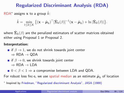
Regularized Discriminant Analysis (RDA)
RDA∗ assigns x to a group k:
k = min1≤k≤K
{(x− µk)
>[Σk(β)]−1(x− µk) + ln |Σk(β)|}.
where Σk(β) are the penalized estimators of scatter matrices obtainedeither using Proposal 1 or Proposal 2.
Interpretation:
if β → 1, we do not shrink towards joint center⇒ RDA → QDA
if β → 0, we shrink towards joint center⇒ RDA → LDA
0 < β < 1 ⇒ a compromise between LDA and QDA.
For robust loss fnc-s, we use spatial median as an estimate µk of location
∗ Inspired by Friedman, ”Regularized discriminant Analysis”, JASA (1989)
Applications Regularized discriminant analysis Esa Ollila 99 / 114
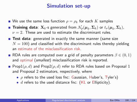
Simulation set-up
We use the same loss function ρ = ρk for each K samples
Training data: Xk-s generated from Np(µk,Σk) or tν(µk,Σk),ν = 2. These are used to estimate the discriminant rules.
Test data: generated in exactly the same manner (same sizeN = 100) and classified with the discriminant rules thereby yieldingan estimate of the misclassification risk.
RDA rules are computed over a grid of penalty parameters β ∈ (0, 1)and optimal (smallest) misclassification risk is reported.
Prop1(ρ, d) and Prop2(ρ, d) refer to RDA rules based on Proposal 1and Proposal 2 estimators, respectively, where
• ρ refers to the used loss fnc: Gaussian, Huber’s, Tyler’s)• d refers to the used distance fnc: (KL or Ellipticity).
Applications Regularized discriminant analysis Esa Ollila 100 / 114
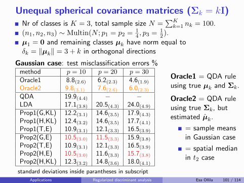
Unequal spherical covariance matrices (Σk = kI)Nr of classes is K = 3, total sample size N =
∑Kk=1 nk = 100.
(n1, n2, n3) ∼ Multin(N ; p1 = p2 = 14 , p3 = 1
2).
µ1 = 0 and remaining classes µk have norm equal toδk = ‖µk‖ = 3 + k in orthogonal directions
Gaussian case: test misclassification errors %method p = 10 p = 20 p = 30Oracle1 8.8(2.6) 6.2(2.3) 4.6(1.9)
Oracle2 9.8(3.1) 7.6(2.6) 6.0(2.3)
QDA 19.9(4.4) − −LDA 17.1(3.8) 20.5(4.3) 24.0(4.9)
Prop1(G,KL) 12.2(3.1) 14.6(3.5) 17.9(4.3)
Prop1(H,KL) 12.4(3.2) 14.6(3.5) 17.7(4.1)
Prop1(T,E) 10.9(3.1) 12.1(3.3) 16.5(3.9)
Prop2(G,E) 10.5(3.0) 11.5(3.3) 15.9(3.8)
Prop2(T,E) 10.9(3.1) 12.1(3.3) 16.5(3.9)
Prop2(H,E) 10.5(3.0) 11.6(3.3) 15.7(3.8)
Prop2(H,KL) 12.3(3.2) 14.8(3.6) 18.0(4.1)
standard deviations inside parantheses in subscript
Oracle1 = QDA ruleusing true µk and Σk.
Oracle2 = QDA ruleusing true Σk, butestimated µk.
= sample meansin Gaussian case
= spatial medianin t2 case
Applications Regularized discriminant analysis Esa Ollila 101 / 114
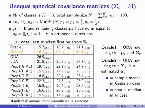
Unequal spherical covariance matrices (Σk = kI)
Nr of classes is K = 3, total sample size N =∑K
k=1 nk = 100.
(n1, n2, n3) ∼ Multin(N ; p1 = p2 = 14 , p3 = 1
2).
µ1 = 0 and remaining classes µk have norm equal toδk = ‖µk‖ = 4 + k in orthogonal directions
t2 case: test misclassification errors %Oracle1 15.7(3.8) 18.2(3.9) 21.1(4.0)
Oracle2 16.2(3.5) 19.1(4.2) 21.9(4.1)
QDA 26.9(5.2) − −LDA 21.8(4.9) 25.3(5.3) 27.7(5.3)
Prop1(G,KL) 19.7(4.8) 22.7(5.2) 24.7(5.1)
Prop1(H,KL) 15.5(3.7) 17.9(4.0) 20.3(4.1)
Prop1(T,E) 16.8(4.0) 20.4(4.3) 23.4(4.7)
Prop2(G,E) 22.3(5.9) 24.3(5.1) 25.9(4.8)
Prop2(T,E) 16.8(4.0) 20.4(4.4) 23.5(4.8)
Prop2(H,E) 16.6(3.9) 20.2(4.4) 23.6(4.6)
Prop2(H,KL) 15.5(3.7) 17.9(4.0) 20.5(4.1)
standard deviations inside parantheses in subscript
Oracle1 = QDA ruleusing true µk and Σk.
Oracle2 = QDA ruleusing true Σk, butestimated µk:
= sample meansin Gaussian case
= spatial medianin t2 case
Applications Regularized discriminant analysis Esa Ollila 102 / 114
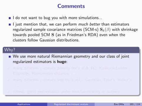
Comments
I do not want to bug you with more simulations...
I just mention that, we can perform much better than estimatorsregularized sample covariance matrices (SCM-s) Sk(β) with shrinkagetowards pooled SCM S (as in Friedman’s RDA) even when theclusters follow Gaussian distributions.
Why?
We use more natural Riemannian geometry and our class of jointregularized estimators is huge:
X many different g-convex penalty fnc’s d(A,B): Kullback-Leibler ,Ellipticity, Riemannian distance, . . .
X many different g-convex loss fnc’s ρ(t): Gaussian, Tyler’s, Huber’s,. . ..
X robust: good performance under non-Gaussianity or outliers
Applications Regularized discriminant analysis Esa Ollila 103 / 114
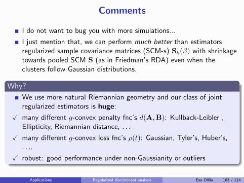
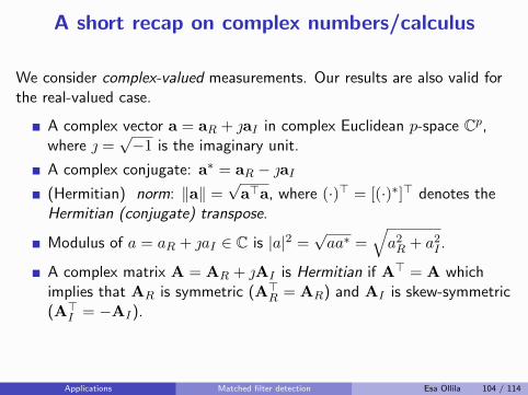
A short recap on complex numbers/calculus
We consider complex-valued measurements. Our results are also valid forthe real-valued case.
A complex vector a = aR + aI in complex Euclidean p-space Cp,where =
√−1 is the imaginary unit.
A complex conjugate: a∗ = aR − aI(Hermitian) norm: ‖a‖ =
√a>a, where (·)> = [(·)∗]> denotes the
Hermitian (conjugate) transpose.
Modulus of a = aR + aI ∈ C is |a|2 =√aa∗ =
√a2R + a2I .
A complex matrix A = AR + AI is Hermitian if A> = A whichimplies that AR is symmetric (A>R = AR) and AI is skew-symmetric(A>I = −AI).
Applications Matched filter detection Esa Ollila 104 / 114
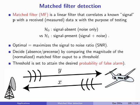
Matched filter detection
Matched filter (MF) is a linear filter that correlates a known ”signal”p with a received (measured) data x with the purpose of testing
H0 : signal-absent (noise only)
vs H1 : signal-present (signal + noise) .
Optimal = maximizes the signal to noise ratio (SNR).
Decide (absence/precense) by comparing the magnitude of the(normalized) matched filter ouput to a threshold.
Threshold is set to attain the desired probability of false alarm).
Applications Matched filter detection Esa Ollila 105 / 114
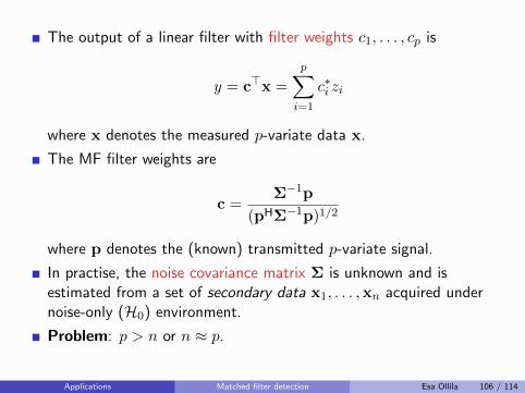
The output of a linear filter with filter weights c1, . . . , cp is
y = c>x =
p∑
i=1
c∗i zi
where x denotes the measured p-variate data x.
The MF filter weights are
c =Σ−1p
(pHΣ−1p)1/2
where p denotes the (known) transmitted p-variate signal.
In practise, the noise covariance matrix Σ is unknown and isestimated from a set of secondary data x1, . . . ,xn acquired undernoise-only (H0) environment.
Problem: p > n or n ≈ p.
Applications Matched filter detection Esa Ollila 106 / 114
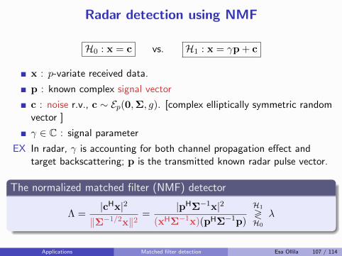
Radar detection using NMF
H0 : x = c vs. H1 : x = γp + c
x : p-variate received data.
p : known complex signal vector
c : noise r.v., c ∼ Ep(0,Σ, g). [complex elliptically symmetric randomvector ]
γ ∈ C : signal parameter
EX In radar, γ is accounting for both channel propagation effect andtarget backscattering; p is the transmitted known radar pulse vector.
The normalized matched filter (NMF) detector
Λ =|cHx|2‖Σ−1/2x‖2
=|pHΣ−1x|2
(xHΣ−1x)(pHΣ−1p)
H1
≷H0
λ
Applications Matched filter detection Esa Ollila 107 / 114
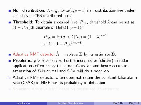
Null distribution: Λ ∼H0 Beta(1, p− 1) i.e., distribution-free underthe class of CES distributed noise.
Threshold: To obtain a desired level PFA, threshold λ can be set as(1− PFA)th quantile of Beta(1, p− 1):
PFA = Pr(Λ > λ|H0) = (1− λ)p−1
⇒ λ = 1− PFA1/(p−1).
Adaptive NMF detector Λ = replace Σ by its estimate Σ.
Problems: p > n or n ≈ p. Furthermore, noise (clutter) in radarapplications often heavy-tailed non-Gaussian and hence accurateestimation of Σ is crucial and SCM will do a poor job.
⇒ Adaptive NMF detector often does not retain the constant false alarmrate (CFAR) of NMF nor its probability of detection
Solution: Adaptive NMF based on regularized M -estimator
Applications Matched filter detection Esa Ollila 108 / 114
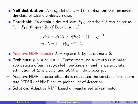
Simulation set-up
Q: How well does the adaptive NMF detector Λ based on estimated Σmaintain the preset PFA?
Simulation set-up: H0 holds, and x = c ∼ CKp,ν(0,Σ)
received data x (input for the NMF detector)
secondary data x1, . . . ,xn (input to estimate Σ).
p = 8 and the shape parameter of the K-distribution is ν = 4.5.
For 10000 trials, we calculated the empirical PFA for fixed λ where thetrue covariance matrix Σ was generated randomly for each trial.
Applications Matched filter detection Esa Ollila 109 / 114
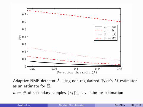
0.32 0.36 0.4 0.44 0.480
0.1
0.2
0.3
0.4
0.5
0.6
0.7
PFA
Detect ion threshold (λ )
n = ∞
n = 8n = 16n = 32
Adaptive NMF detector Λ using non-regularized Tyler’s M -estimatoras an estimate for Σ.
n := # of secondary samples {xi}ni=1 availabe for estimation
Applications Matched filter detection Esa Ollila 110 / 114
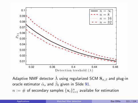
0.32 0.36 0.4 0.44 0.48
0.01
0.02
0.03
0.04
0.05
0.06
0.07
0.08
0.09
0.1
PFA
Detect ion treshold (λ )
n = ∞
n = 8n = 16n = 32
Adaptive NMF detector Λ using regularized SCM Sα,β and plug-in
oracle estimator αo and β0 given in Slide 91.
n := # of secondary samples {xi}ni=1 availabe for estimation
Applications Matched filter detection Esa Ollila 111 / 114
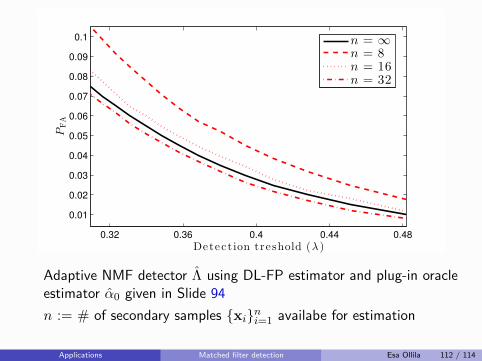
0.32 0.36 0.4 0.44 0.48
0.01
0.02
0.03
0.04
0.05
0.06
0.07
0.08
0.09
0.1
PFA
Detect ion treshold (λ )
n = ∞
n = 8n = 16n = 32
Adaptive NMF detector Λ using DL-FP estimator and plug-in oracleestimator α0 given in Slide 94
n := # of secondary samples {xi}ni=1 availabe for estimation
Applications Matched filter detection Esa Ollila 112 / 114
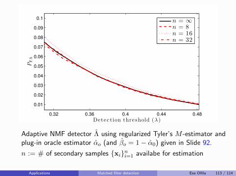
0.32 0.36 0.4 0.44 0.48
0.01
0.02
0.03
0.04
0.05
0.06
0.07
0.08
0.09
0.1
PFA
Detect ion threshold (λ )
n = ∞
n = 8n = 16n = 32
Adaptive NMF detector Λ using regularized Tyler’s M -estimator andplug-in oracle estimator αo (and βo = 1− α0) given in Slide 92.
n := # of secondary samples {xi}ni=1 availabe for estimation
Applications Matched filter detection Esa Ollila 113 / 114

Thank you !!!
References: see the next slides
Applications Matched filter detection Esa Ollila 114 / 114
Abramovich, Y. and Besson, O. (2013).
Regularized covariance matrix estimation in complex elliptically symmetricdistributions using the expected likelihood approach-part 1: The over-sampled case.
IEEE Trans. Signal Process., 61(23):5807–5818.
Abramovich, Y. I. and Spencer, N. K. (2007).
Diagonally loaded normalised sample matrix inversion (LNSMI) for outlier-resistantadaptive filtering.
In Proc. Int’l Conf. on Acoustics, Speech and Signal Processing (ICASSP’07),pages 1105–1108.
Besson, O. and Abramovich, Y. (2013).
Regularized covariance matrix estimation in complex elliptically symmetricdistributions using the expected likelihood approach-part 2: The under-sampledcase.
IEEE Trans. Signal Process., 61(23):5819–5829.
Bhatia, R. (2009).
Positive definite matrices.
Princeton University Press.
Chen, Y., Wiesel, A., and Hero, A. O. (2011).
Robust shrinkage estimation of high-dimensional covariance matrices.
IEEE Trans. Signal Process., 59(9):4097 – 4107.
Conte, E., De Maio, A., and Ricci, G. (2002).
Recursive estimation of the covariance matrix of a compound-Gaussian process andits application to adaptive CFAR detection.
IEEE Trans. Signal Process., 50(8):1908 – 1915.
Cover, T. M. and Thomas, J. A. (2012).
Elements of information theory.
John Wiley & Sons.
Du, L., Li, J., and Stoica, P. (2010).
Fully automatic computation of diagonal loading levels for robust adaptivebeamforming.
IEEE Trans. Aerosp. Electron. Syst., 46(1):449–458.
Friedman, J., Hastie, T., and Tibshirani, R. (2008).
Sparse inverse covariance estimation with the graphical lasso.
Biostatistics, 9(3):432–441.
Friedman, J. H. (1989).
Regularized discriminant analysis.
J. Amer. Stat. Assoc., 84(405):165–175.
Gini, F. and Greco, M. (2002).
Covariance matrix estimation for CFAR detection in correlated heavy-tailed clutter.
Signal Processing, 82(12):1847–1859.
Kent, J. T. (1997).
Data analysis for shapes and images.
J. Statist. Plann. Inference, 57(2):181–193.
Ledoit, O. and Wolf, M. (2004).
A well-conditioned estimator for large-dimensional covariance matrices.
J. Mult. Anal., 88:365–411.
Maronna, R. A. (1976).
Robust M-estimators of multivariate location and scatter.
Ann. Stat., 5(1):51–67.
Ollila, E., Soloveychik, I., Tyler, D. E., and Wiesel, A. (2016).
Simultaneous penalized M-estimation of covariance matrices using geodesicallyconvex optimization.
Journal of Multivariate Analysis, submitted.
Ollila, E. and Tyler, D. E. (2012).
Distribution-free detection under complex elliptically symmetric clutter distribution.
In Proc. IEEE Sensor Array and Multichannel Signal Processing Workshop(SAM’12), Hoboken, NJ, USA.
Ollila, E. and Tyler, D. E. (2014).
Regularized M -estimators of scatter matrix.
IEEE Trans. Signal Process., 62(22):6059–6070.
Pascal, F., Chitour, Y., and Quek, Y. (2014).
Generalized robust shrinkage estimator and its application to stap detectionproblem.
IEEE Trans. Signal Process., 62(21):5640–5651.
Sra, S. (2011).
Positive definite matrices and the S-divergence.
arXiv preprint arXiv:1110.1773.
Sun, Y., Babu, P., and Palomar, D. P. (2014).
Regularized tyler’s scatter estimator: Existence, uniqueness, and algorithms.
IEEE Trans. Signal Process., 62(19):5143–5156.
Wiesel, A. (2012).
Unified framework to regularized covariance estimation in scaled gaussian models.
IEEE Trans. Signal Process., 60(1):29–38.
Wiesel, A. and Zhang, T. (2015).
Structured robust covariance estimation.
Foundations and Trends in Signal Processing, 8(3):127–216.
Zhang, T., Wiesel, A., and Greco, M. S. (2013).
Multivariate generalized Gaussian distribution: Convexity and graphical models.
IEEE Trans. Signal Process., 61(16):4141–4148.
Applications Matched filter detection Esa Ollila 114 / 114
![Modern Computational Statistics [1em] Lecture 2: Optimization · 2020-05-27 · Regularized Regression Models 3/38 I In practice, we would like to solve the least square problems](https://static.fdocument.org/doc/165x107/5f17a4228f70f05e381f922b/modern-computational-statistics-1em-lecture-2-optimization-2020-05-27-regularized.jpg)


![Gaussian Graphical Models and Graphical Lassoyc5/ele538b_sparsity/lectures/... · 2018-11-07 · [1]”Sparse inverse covariance estimation with the graphical lasso,” J. Friedman,](https://static.fdocument.org/doc/165x107/5ecf277214450a5e2f099e28/gaussian-graphical-models-and-graphical-yc5ele538bsparsitylectures-2018-11-07.jpg)