The Split Bregman Method for L1-Regularized Problemspopov/L12008/talks/L1presentation.pdf · The...
28
The Split Bregman Method for L1-Regularized Problems Tom Goldstein May 22, 2008
-
Upload
dangnguyet -
Category
Documents
-
view
241 -
download
0
Transcript of The Split Bregman Method for L1-Regularized Problemspopov/L12008/talks/L1presentation.pdf · The...
The Split Bregman Method for L1-RegularizedProblems
Tom Goldstein
May 22, 2008
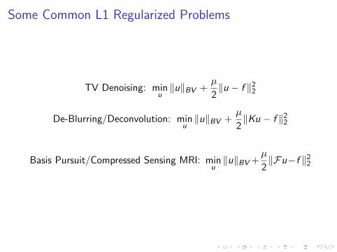
Some Common L1 Regularized Problems
TV Denoising: minu‖u‖BV +
µ
2‖u − f ‖22
De-Blurring/Deconvolution: minu‖u‖BV +
µ
2‖Ku − f ‖22
Basis Pursuit/Compressed Sensing MRI: minu‖u‖BV +
µ
2‖Fu−f ‖22
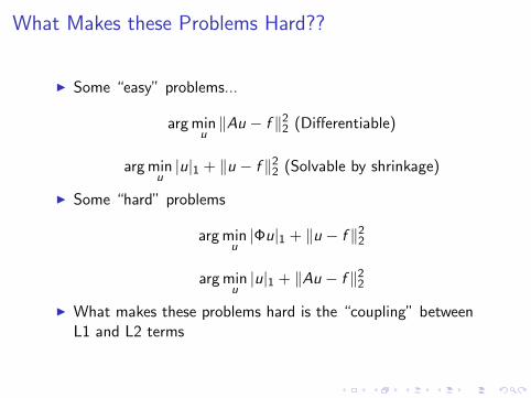
What Makes these Problems Hard??
I Some “easy” problems...
arg minu‖Au − f ‖22 (Differentiable)
arg minu|u|1 + ‖u − f ‖22 (Solvable by shrinkage)
I Some “hard” problems
arg minu|Φu|1 + ‖u − f ‖22
arg minu|u|1 + ‖Au − f ‖22
I What makes these problems hard is the “coupling” betweenL1 and L2 terms
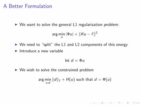
A Better Formulation
I We want to solve the general L1 regularization problem:
arg minu|Φu|+ ‖Ku − f ‖2
I We need to “split” the L1 and L2 components of this energy
I Introduce a new variable
let d = Φu
I We wish to solve the constrained problem
arg minu,d‖d‖1 + H(u) such that d = Φ(u)
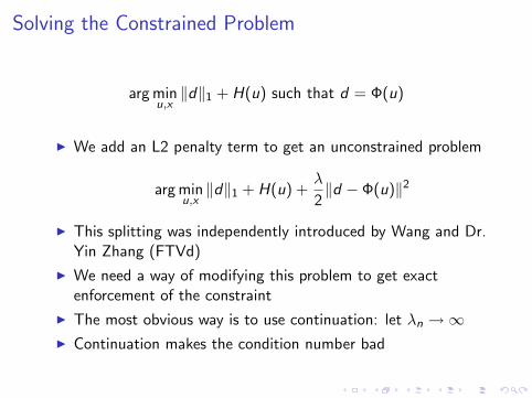
Solving the Constrained Problem
arg minu,x‖d‖1 + H(u) such that d = Φ(u)
I We add an L2 penalty term to get an unconstrained problem
arg minu,x‖d‖1 + H(u) +
λ
2‖d − Φ(u)‖2
I This splitting was independently introduced by Wang and Dr.Yin Zhang (FTVd)
I We need a way of modifying this problem to get exactenforcement of the constraint
I The most obvious way is to use continuation: let λn →∞I Continuation makes the condition number bad
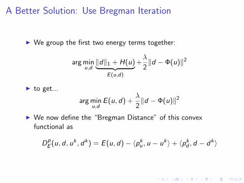
A Better Solution: Use Bregman Iteration
I We group the first two energy terms together:
arg minu,d‖d‖1 + H(u)︸ ︷︷ ︸
E(u,d)
+λ
2‖d − Φ(u)‖2
I to get...
arg minu,d
E (u, d) +λ
2‖d − Φ(u)‖2
I We now define the “Bregman Distance” of this convexfunctional as
DpE (u, d , uk , dk) = E (u, d)− 〈pk
u , u − uk〉+ 〈pkd , d − dk〉
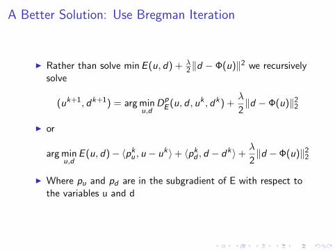
A Better Solution: Use Bregman Iteration
I Rather than solve min E (u, d) + λ2‖d − Φ(u)‖2 we recursively
solve
(uk+1, dk+1) = arg minu,d
DpE (u, d , uk , dk) +
λ
2‖d − Φ(u)‖22
I or
arg minu,d
E (u, d)− 〈pku , u − uk〉+ 〈pk
d , d − dk〉+ λ
2‖d −Φ(u)‖22
I Where pu and pd are in the subgradient of E with respect tothe variables u and d
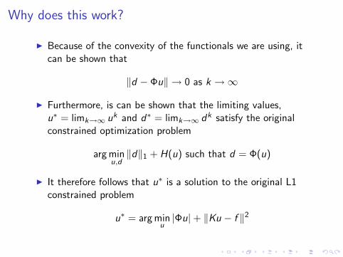
Why does this work?
I Because of the convexity of the functionals we are using, itcan be shown that
‖d − Φu‖ → 0 as k →∞
I Furthermore, is can be shown that the limiting values,u∗ = limk→∞ uk and d∗ = limk→∞ dk satisfy the originalconstrained optimization problem
arg minu,d‖d‖1 + H(u) such that d = Φ(u)
I It therefore follows that u∗ is a solution to the original L1constrained problem
u∗ = arg minu|Φu|+ ‖Ku − f ‖2
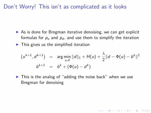
Don’t Worry! This isn’t as complicated as it looks
I As is done for Bregman iterative denoising, we can get explicitformulas for pu and pd , and use them to simplify the iteration
I This gives us the simplified iteration
(uk+1, dk+1) = arg minu,d‖d‖1 + H(u) +
λ
2‖d − Φ(u)− bk‖2
bk+1 = bk + (Φ(u)− dk)
I This is the analog of “adding the noise back” when we useBregman for denoising
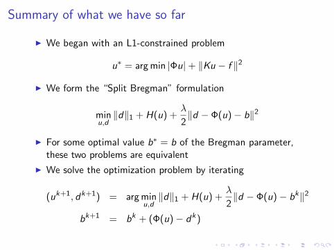
Summary of what we have so far
I We began with an L1-constrained problem
u∗ = arg min |Φu|+ ‖Ku − f ‖2
I We form the “Split Bregman” formulation
minu,d‖d‖1 + H(u) +
λ
2‖d − Φ(u)− b‖2
I For some optimal value b∗ = b of the Bregman parameter,these two problems are equivalent
I We solve the optimization problem by iterating
(uk+1, dk+1) = arg minu,d‖d‖1 + H(u) +
λ
2‖d − Φ(u)− bk‖2
bk+1 = bk + (Φ(u)− dk)
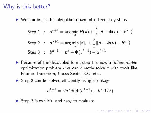
Why is this better?
I We can break this algorithm down into three easy steps
Step 1 : uk+1 = arg minu
H(u) +λ
2‖d − Φ(u)− bk‖22
Step 2 : dk+1 = arg mind|d |1 +
λ
2‖d − Φ(u)− bk‖22
Step 3 : bk+1 = bk + Φ(uk+1)− dk+1
I Because of the decoupled form, step 1 is now a differentiableoptimization problem - we can directly solve it with tools likeFourier Transform, Gauss-Seidel, CG, etc...
I Step 2 can be solved efficiently using shrinkage
dk+1 = shrink(Φ(uk+1) + bk , 1/λ)
I Step 3 is explicit, and easy to evaluate
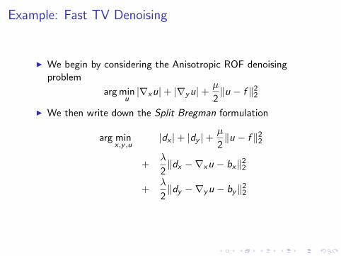
Example: Fast TV Denoising
I We begin by considering the Anisotropic ROF denoisingproblem
arg minu|∇xu|+ |∇yu|+ µ
2‖u − f ‖22
I We then write down the Split Bregman formulation
arg minx ,y ,u
|dx |+ |dy |+µ
2‖u − f ‖22
+λ
2‖dx −∇xu − bx‖22
+λ
2‖dy −∇yu − by‖22
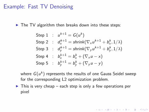
Example: Fast TV Denoising
I The TV algorithm then breaks down into these steps:
Step 1 : uk+1 = G (uk)
Step 2 : dk+1x = shrink(∇xu
k+1 + bkx , 1/λ)
Step 3 : dk+1y = shrink(∇yuk+1 + bk
y , 1/λ)
Step 4 : bk+1x = bk
x + (∇xu − x)
Step 5 : bk+1y = bk
y + (∇yu − y)
where G (uk) represents the results of one Gauss Seidel sweepfor the corresponding L2 optimization problem.
I This is very cheap – each step is only a few operations perpixel
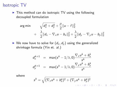
Isotropic TV
I This method can do isotropic TV using the followingdecoupled formulation
arg min√
d2x + d2
y +µ
2‖u − f ‖22
+λ
2‖dx −∇xu − bx‖22 +
λ
2‖dy −∇yu − by‖22
I We now have to solve for (dx , dy ) using the generalizedshrinkage formula (Yin et. al.)
dk+1x = max(sk − 1/λ, 0)
∇xuk + bk
x
sk
dk+1y = max(sk − 1/λ, 0)
∇yuk + bky
sk
wheresk =
√(∇xuk + bk
x )2 + (∇yuk + bky )2
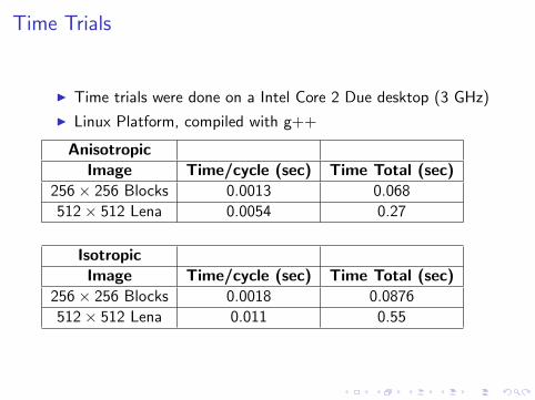
Time Trials
I Time trials were done on a Intel Core 2 Due desktop (3 GHz)
I Linux Platform, compiled with g++
AnisotropicImage Time/cycle (sec) Time Total (sec)
256× 256 Blocks 0.0013 0.068
512× 512 Lena 0.0054 0.27
IsotropicImage Time/cycle (sec) Time Total (sec)
256× 256 Blocks 0.0018 0.0876
512× 512 Lena 0.011 0.55
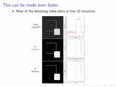
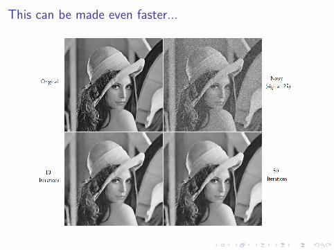
This can be made even faster...I Most of the denoising takes place in first 10 iterations
This can be made even faster...
I Most of the denoising takes place in first 10 iterations
I “Staircases” form quickly, but then take some time to flattenout
I If we are willing to accept a “visual” convergence criteria, wecan denoise in about 10 iterations (0.054 sec) for Lena, and20 iterations (0.024 sec) for the blocky image.
This can be made even faster...
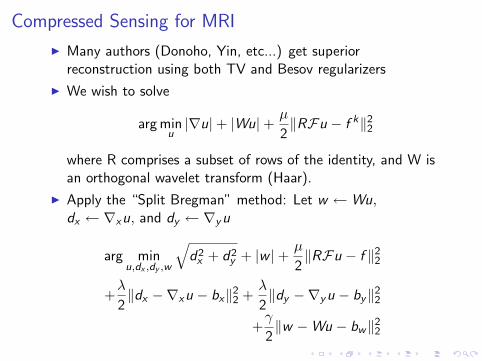
Compressed Sensing for MRI
I Many authors (Donoho, Yin, etc...) get superiorreconstruction using both TV and Besov regularizers
I We wish to solve
arg minu|∇u|+ |Wu|+ µ
2‖RFu − f k‖22
where R comprises a subset of rows of the identity, and W isan orthogonal wavelet transform (Haar).
I Apply the “Split Bregman” method: Let w ←Wu,dx ← ∇xu, and dy ← ∇yu
arg minu,dx ,dy ,w
√d2x + d2
y + |w |+ µ
2‖RFu − f ‖22
+λ
2‖dx −∇xu − bx‖22 +
λ
2‖dy −∇yu − by‖22
+γ
2‖w −Wu − bw‖22
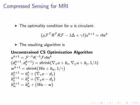
Compressed Sensing for MRI
I The optimality condition for u is circulant:
(µFTRTRF − λ∆ + γI )uk+1 = rhsk
I The resulting algorithm is
Unconstrained CS Optimization Algorithmuk+1 = F−1K−1Frhsk
(dk+1x , dk+1
y ) = shrink(∇xu + bx ,∇yu + by , 1/λ)
wk+1 = shrink(Wu + bw , 1/γ)bk+1x = bk
x + (∇xu − dx)bk+1y = bk
y + (∇yu − dy )
bk+1w = bk
w + (Wu − w)
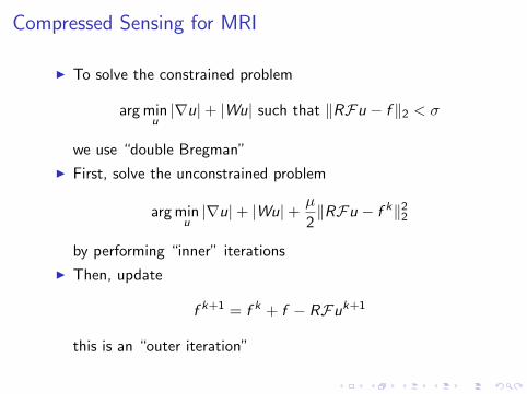
Compressed Sensing for MRI
I To solve the constrained problem
arg minu|∇u|+ |Wu| such that ‖RFu − f ‖2 < σ
we use “double Bregman”
I First, solve the unconstrained problem
arg minu|∇u|+ |Wu|+ µ
2‖RFu − f k‖22
by performing “inner” iterations
I Then, update
f k+1 = f k + f − RFuk+1
this is an “outer iteration”
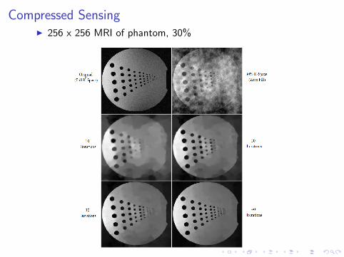
Compressed SensingI 256 x 256 MRI of phantom, 30%
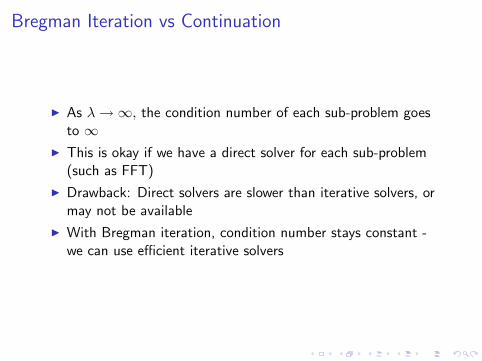
Bregman Iteration vs Continuation
I As λ→∞, the condition number of each sub-problem goesto ∞
I This is okay if we have a direct solver for each sub-problem(such as FFT)
I Drawback: Direct solvers are slower than iterative solvers, ormay not be available
I With Bregman iteration, condition number stays constant -we can use efficient iterative solvers
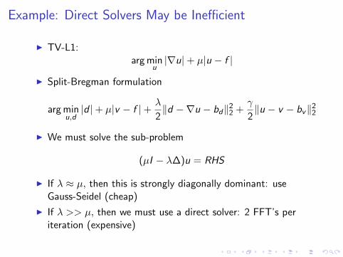
Example: Direct Solvers May be Inefficient
I TV-L1:arg min
u|∇u|+ µ|u − f |
I Split-Bregman formulation
arg minu,d|d |+ µ|v − f |+ λ
2‖d −∇u − bd‖22 +
γ
2‖u − v − bv‖22
I We must solve the sub-problem
(µI − λ∆)u = RHS
I If λ ≈ µ, then this is strongly diagonally dominant: useGauss-Seidel (cheap)
I If λ >> µ, then we must use a direct solver: 2 FFT’s periteration (expensive)
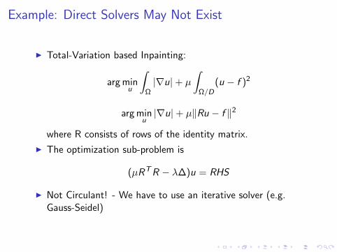
Example: Direct Solvers May Not Exist
I Total-Variation based Inpainting:
arg minu
∫Ω|∇u|+ µ
∫Ω/D
(u − f )2
arg minu|∇u|+ µ‖Ru − f ‖2
where R consists of rows of the identity matrix.
I The optimization sub-problem is
(µRTR − λ∆)u = RHS
I Not Circulant! - We have to use an iterative solver (e.g.Gauss-Seidel)
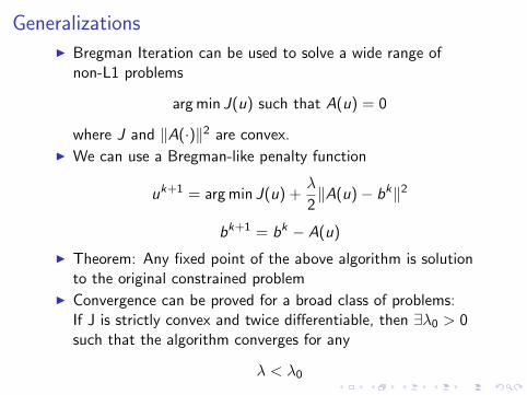
Generalizations
I Bregman Iteration can be used to solve a wide range ofnon-L1 problems
arg min J(u) such that A(u) = 0
where J and ‖A(·)‖2 are convex.I We can use a Bregman-like penalty function
uk+1 = arg min J(u) +λ
2‖A(u)− bk‖2
bk+1 = bk − A(u)
I Theorem: Any fixed point of the above algorithm is solutionto the original constrained problem
I Convergence can be proved for a broad class of problems:If J is strictly convex and twice differentiable, then ∃λ0 > 0such that the algorithm converges for any
λ < λ0
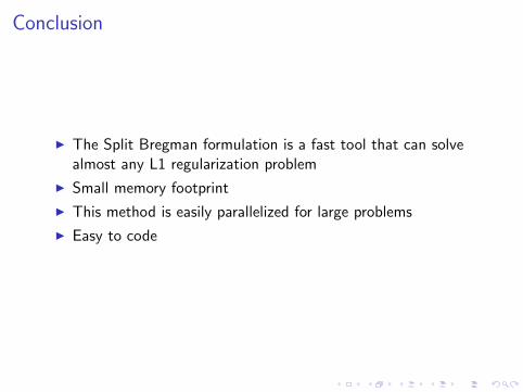
Conclusion
I The Split Bregman formulation is a fast tool that can solvealmost any L1 regularization problem
I Small memory footprint
I This method is easily parallelized for large problems
I Easy to code
Conclusion
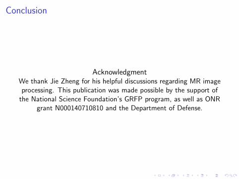
AcknowledgmentWe thank Jie Zheng for his helpful discussions regarding MR imageprocessing. This publication was made possible by the support ofthe National Science Foundation’s GRFP program, as well as ONR
grant N000140710810 and the Department of Defense.