Regression analysisTwo variables 

(Montgomery and Runger: ch 11Brani Vidakovic: ch 14) 

Reminder

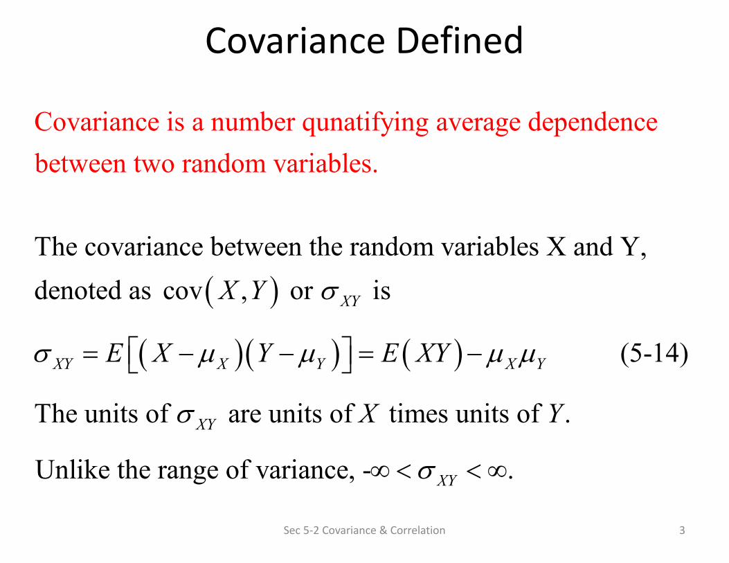
Covariance Defined

Sec 5‐2 Covariance & Correlation 3

The covariance between the random v

Covariance is a number qunatifying

ariables X and Y, denoted as co

average dependence betwee

v , or is

(

n two random variables.

XY

XY X Y X Y

X Y

E X Y E XY

5-14)

The units of are units of times units of .

Unlike the range of variance, - .

XY

XY

X Y

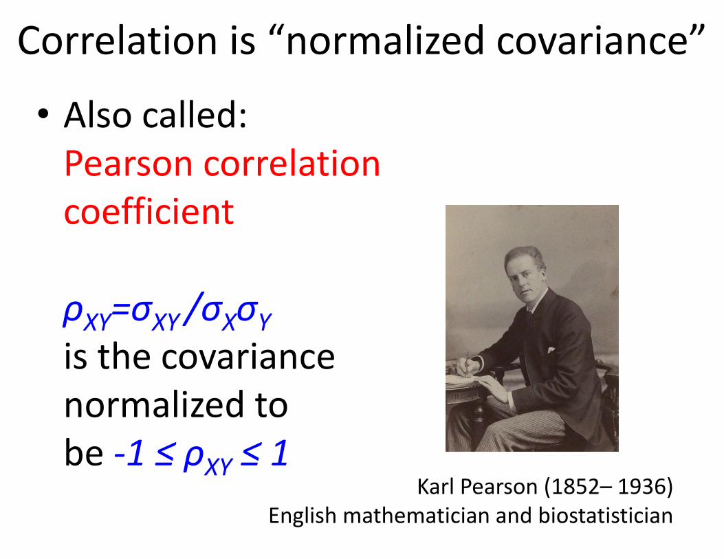
Correlation is “normalized covariance”

• Also called: Pearson correlation coefficient 

ρXY=σXY /σXσYis the covariance normalized to be ‐1 ≤ ρXY ≤ 1

Karl Pearson (1852– 1936) English mathematician and biostatistician

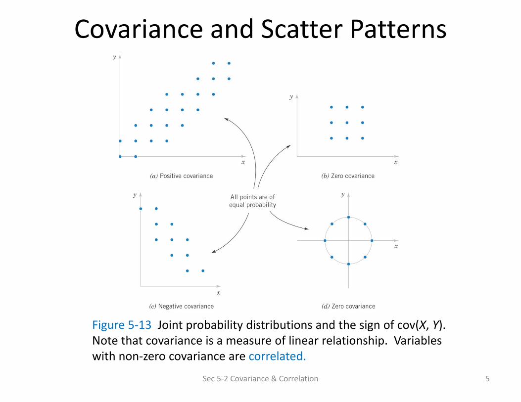
Covariance and Scatter Patterns

Sec 5‐2 Covariance & Correlation 5

Figure 5‐13  Joint probability distributions and the sign of cov(X, Y).  Note that covariance is a measure of linear relationship.  Variables with non‐zero covariance are correlated.

Regression analysis• Many problems in engineering and science involve sample in which two or more variables were measured. They may not be independent from each other and one (or several) of them can be used to predict another

• Everyday example: in most samples height and weight of people are related to each other

• Biological example: in a cell sorting experiment the copy number of a protein may be measured alongside its volume

• Regression analysis uses a sample to build a model to predict protein copy number given a cell volume 6

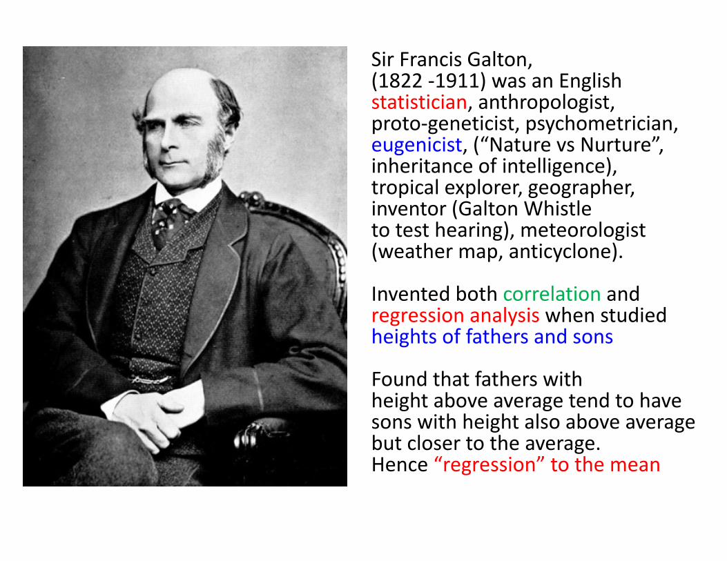
Sir Francis Galton,(1822 ‐1911) was an English statistician, anthropologist, proto‐geneticist, psychometrician, eugenicist, (“Nature vs Nurture”, inheritance of intelligence), tropical explorer, geographer, inventor (Galton Whistle to test hearing), meteorologist (weather map, anticyclone).

Invented both correlation and regression analysis when studied heights of fathers and sons

Found that fathers with height above average tend to havesons with height also above averagebut closer to the average. Hence “regression” to the mean

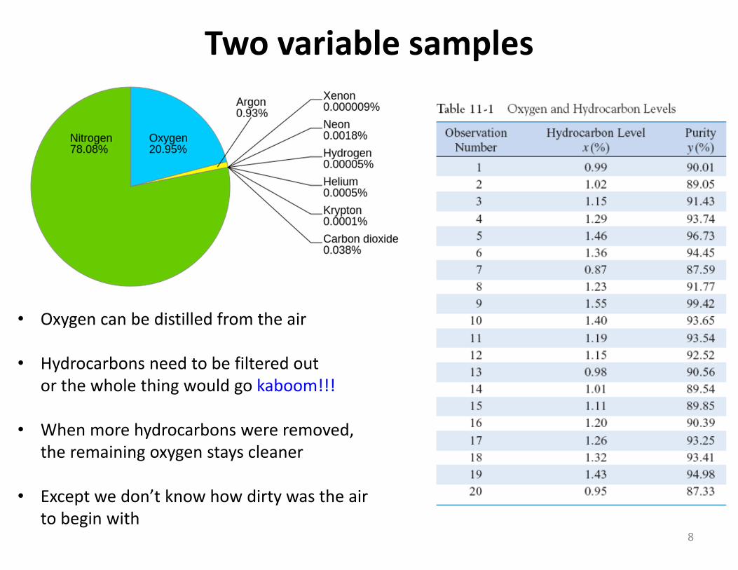
Two variable samples

8

• Oxygen can be distilled from the air

• Hydrocarbons need to be filtered out or the whole thing would go kaboom!!!

• When more hydrocarbons were removed, the remaining oxygen stays cleaner

• Except we don’t know how dirty was the air to begin with

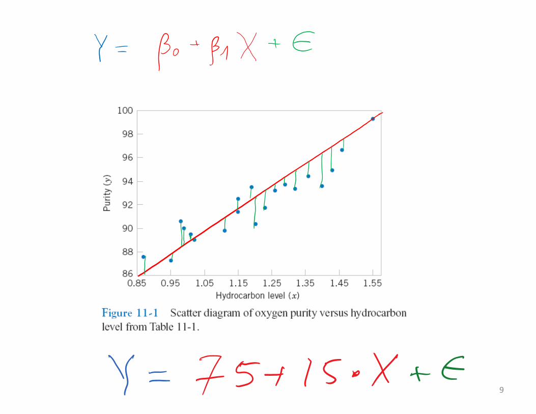
9

Linear regression

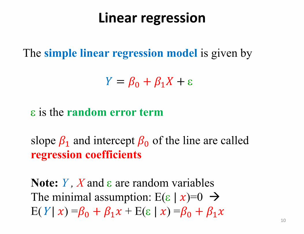
The simple linear regression model is given by

is the random error term

slope and intercept of the line are called regression coefficients

Note: Y , X and are random variablesThe minimal assumption: E( )=0 E( ) = + E( ) =

10

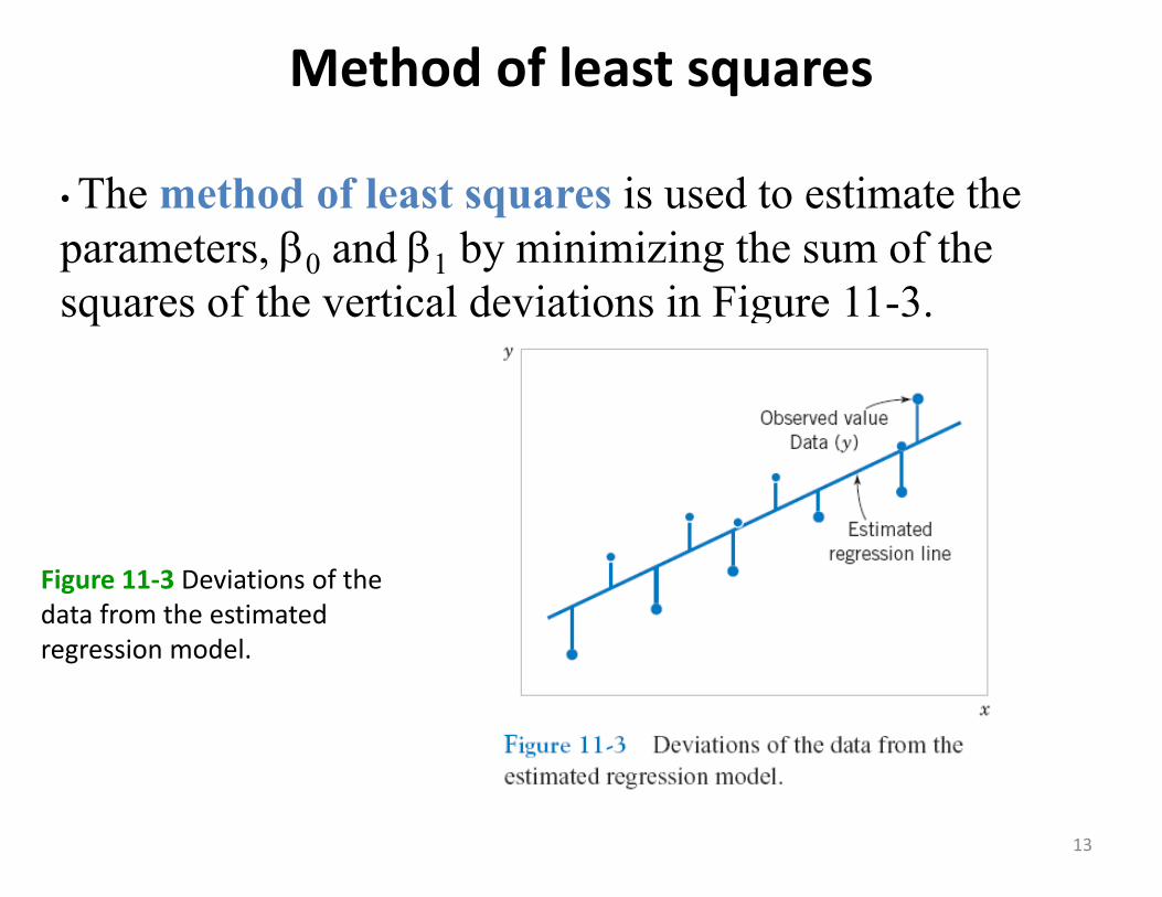
Method of least squares

• The method of least squares is used to estimate the parameters, 0 and 1 by minimizing the sum of the squares of the vertical deviations in Figure 11-3.

Figure 11‐3 Deviations of the data from the estimated regression model.

13

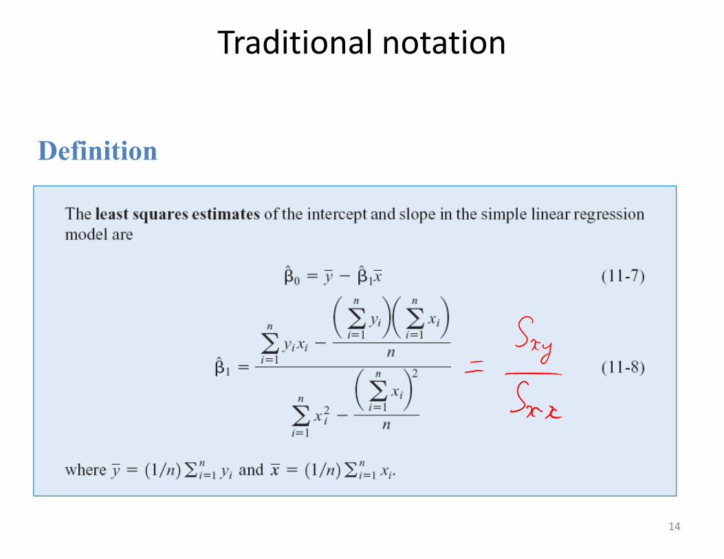
Traditional notation

Definition

14

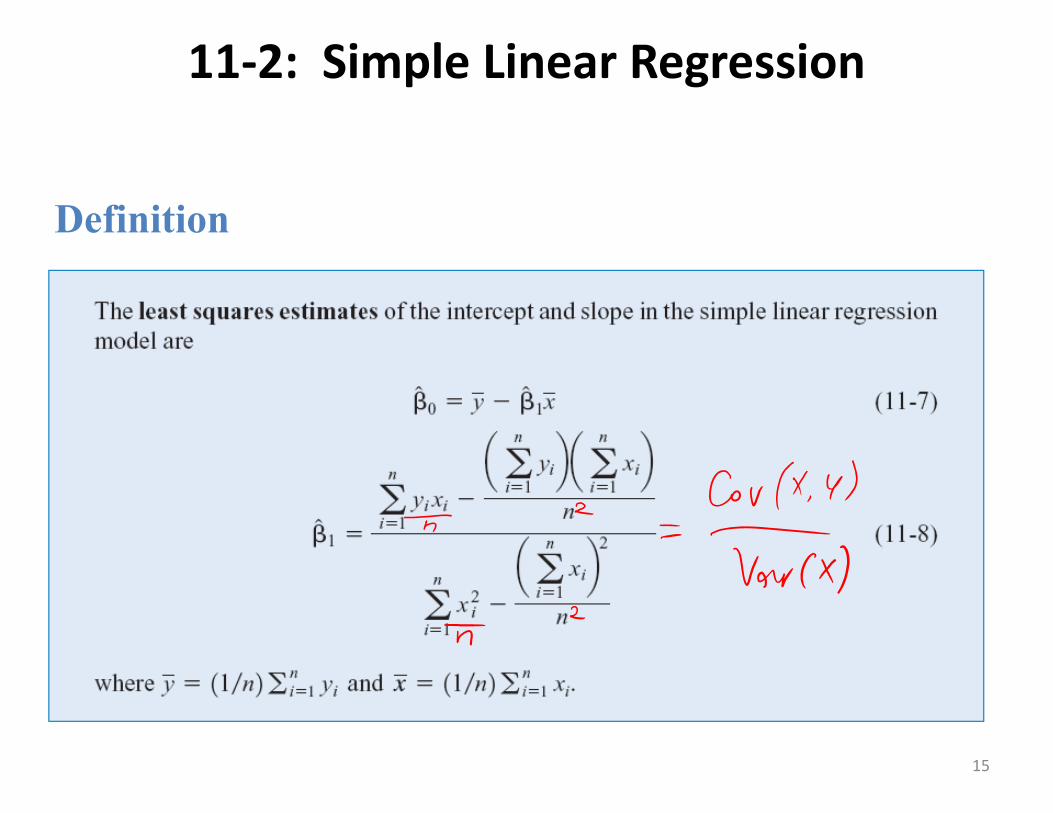
11‐2:  Simple Linear Regression 

Definition

15

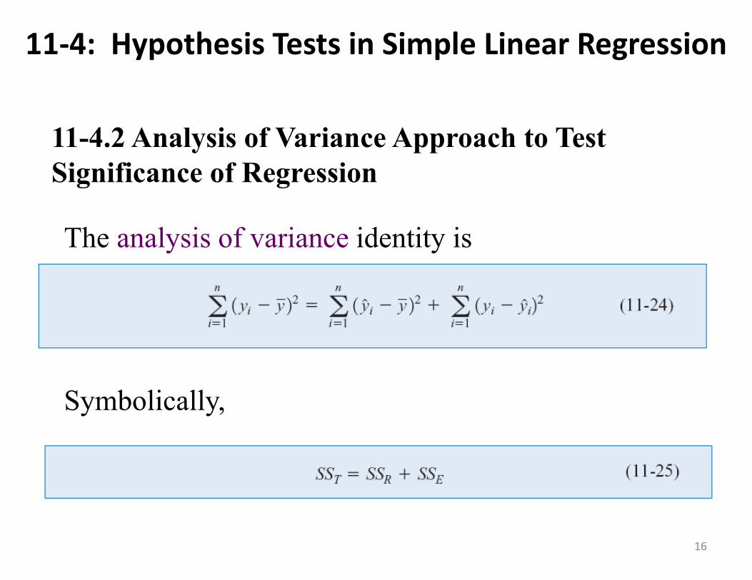
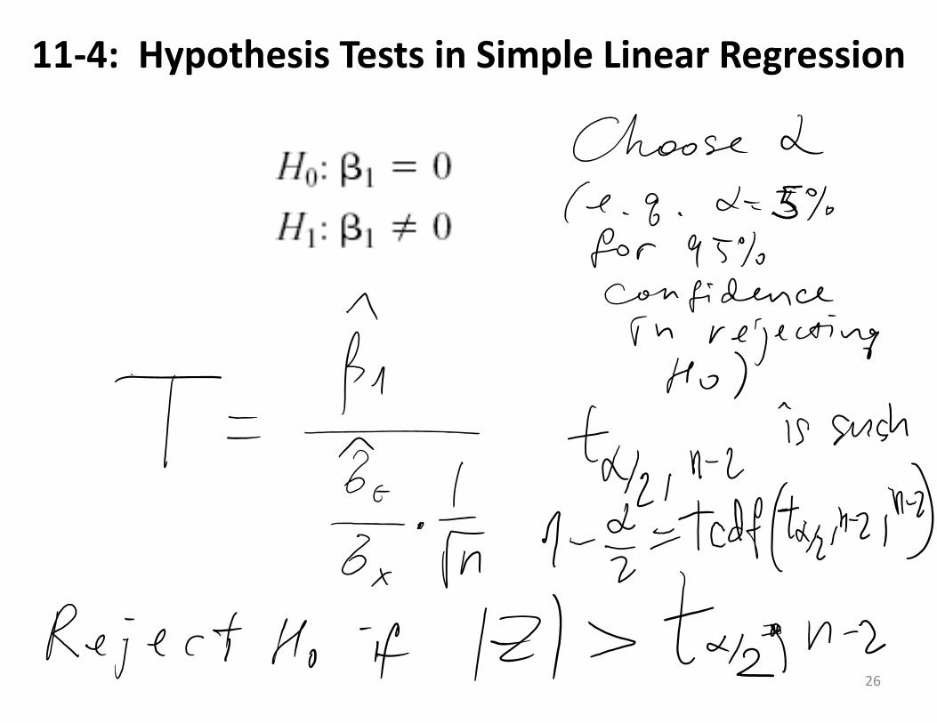
11‐4:  Hypothesis Tests in Simple Linear Regression 

11-4.2 Analysis of Variance Approach to Test Significance of Regression

The analysis of variance identity is

Symbolically,

16

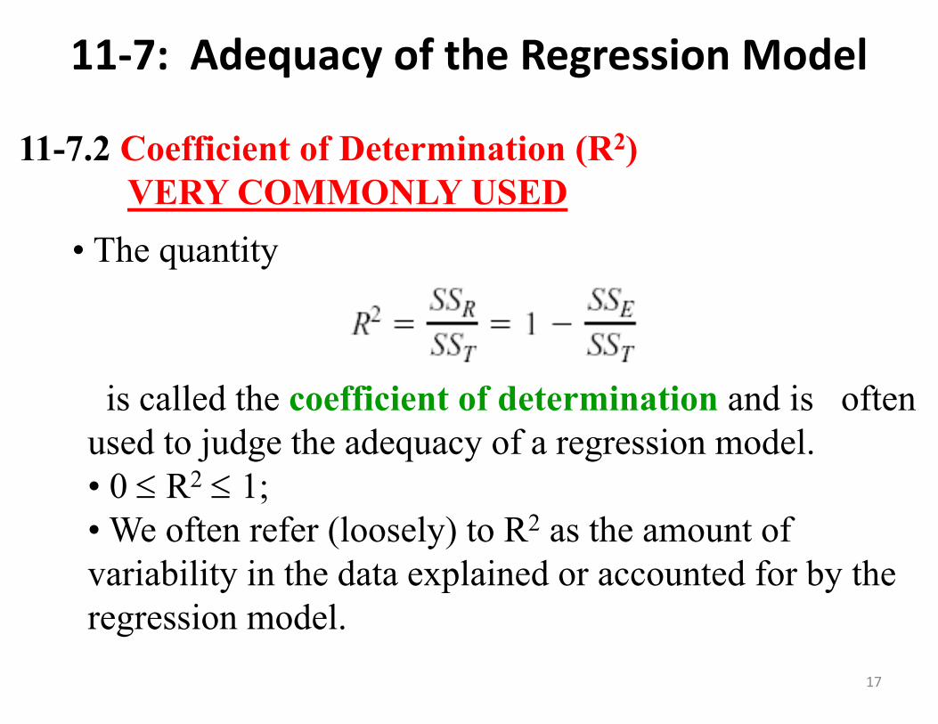
11‐7:  Adequacy of the Regression Model 

11-7.2 Coefficient of Determination (R2) VERY COMMONLY USED

• The quantity

is called the coefficient of determination and is often used to judge the adequacy of a regression model.• 0 R2 1;• We often refer (loosely) to R2 as the amount of variability in the data explained or accounted for by the regression model.

17

11‐7:  Adequacy of the Regression Model 

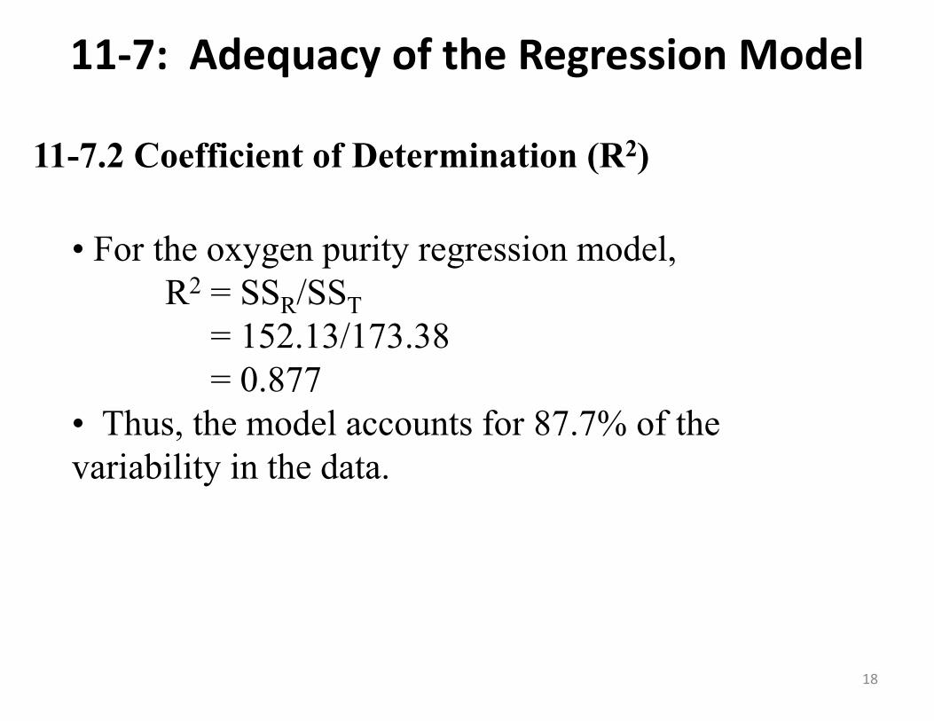
11-7.2 Coefficient of Determination (R2)

• For the oxygen purity regression model, R2 = SSR/SST

= 152.13/173.38 = 0.877

• Thus, the model accounts for 87.7% of the variability in the data.

18

11‐2:  Simple Linear Regression 

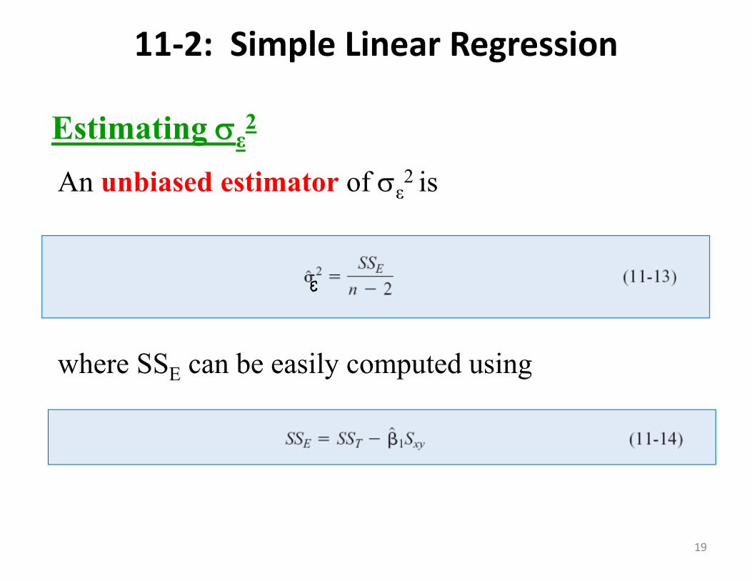
Estimating ε2

An unbiased estimator of ε2 is

where SSE can be easily computed using

19

11‐3:  Properties of the Least Squares Estimators 

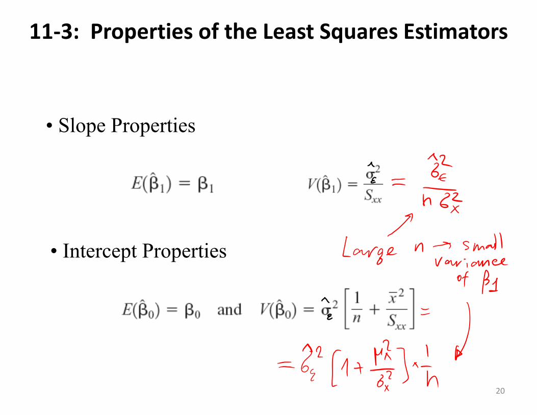
• Slope Properties

• Intercept Properties

20

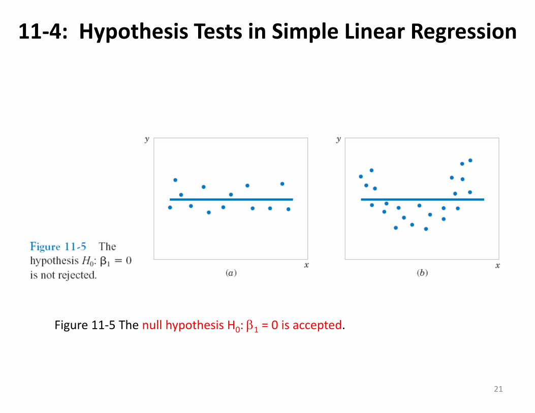
11‐4:  Hypothesis Tests in Simple Linear Regression 

Figure 11‐5 The null hypothesis H0: 1 = 0 is accepted.

21

11‐4:  Hypothesis Tests in Simple Linear Regression 

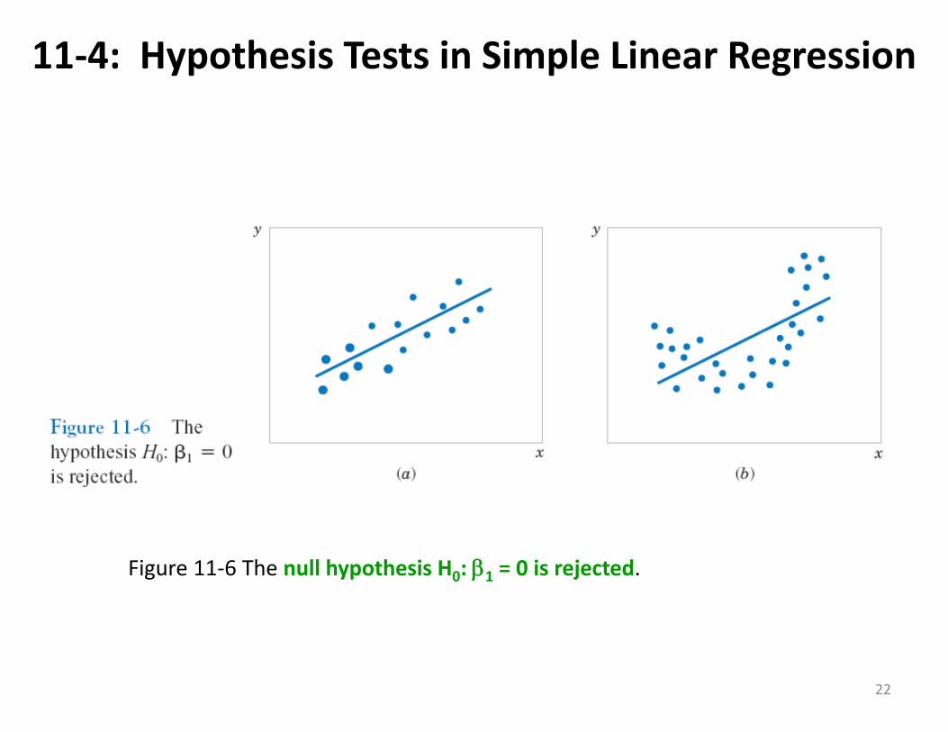
Figure 11‐6 The null hypothesis H0: 1 = 0 is rejected.

22

11‐4:  Hypothesis Tests in Simple Linear Regression 

11-4.1 Use of Z-tests for large n An important special case of the hypotheses of Equation 11-18 is

These hypotheses relate to the significance of regression.Failure to reject H0 is equivalent to concluding that there is no linear relationship between X and Y.

23

11‐4:  Hypothesis Tests in Simple Linear Regression 

24

11‐4:  Hypothesis Tests in Simple Linear Regression 

11-4.1 Use of t-tests for smaller n.

The number of degrees of freedom in n-2

One can always fit a straight line through two points so one needs n>=3

11‐4:  Hypothesis Tests in Simple Linear Regression 

26

Credit: XKCD comics 

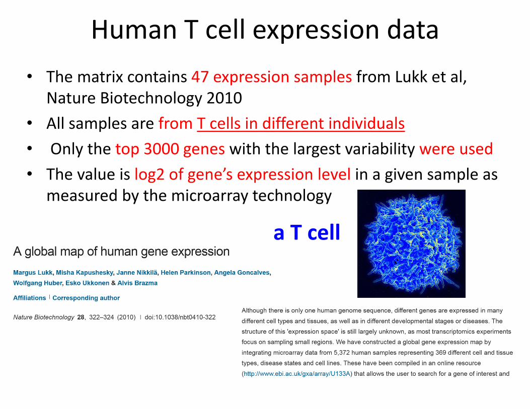
Human T cell expression data• The matrix contains 47 expression samples from Lukk et al, 

Nature Biotechnology 2010• All samples are from T cells in different individuals• Only the top 3000 genes with the largest variability were used• The value is log2 of gene’s expression level in a given sample as 

measured by the microarray technology

• T cellsa T cell 

“Let’s Make a Deal” show with Monty Hall aired on NBC/ABC 1963‐1986

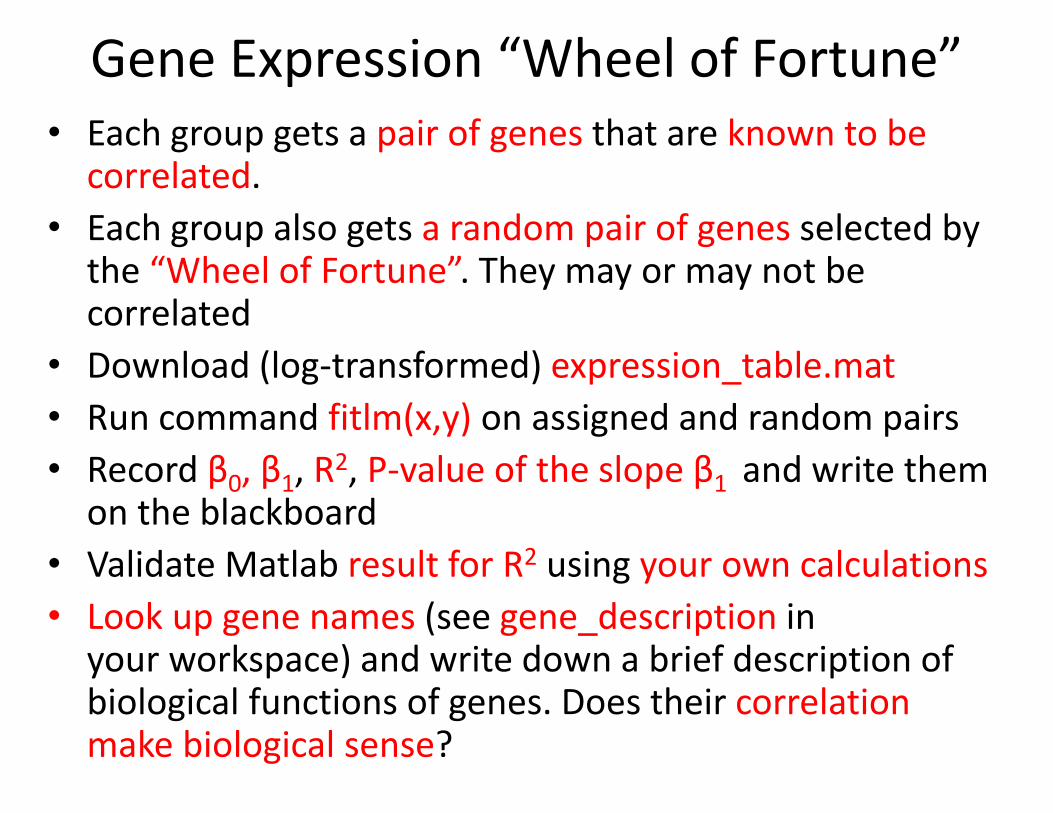
Gene Expression “Wheel of Fortune” • Each group gets a pair of genes that are known to be correlated. 

• Each group also gets a random pair of genes selected by the “Wheel of Fortune”. They may or may not be correlated

• Download (log‐transformed) expression_table.mat• Run command fitlm(x,y) on assigned and random pairs • Record β0, β1, R2, P‐value of the slope β1 and write them on the blackboard

• Validate Matlab result for R2 using your own calculations• Look up gene names (see gene_description in your workspace) and write down a brief description of biological functions of genes. Does their correlation make biological sense?

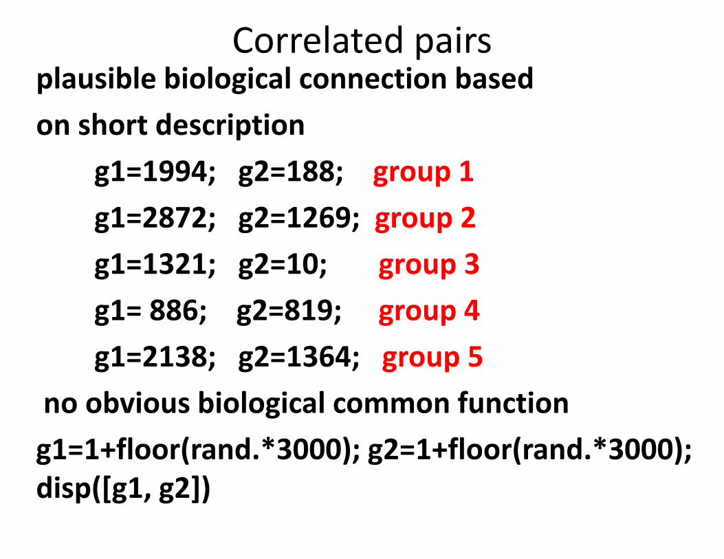
Correlated pairsplausible biological connection based on short description

g1=1994;   g2=188;    group 1g1=2872;   g2=1269;  group 2g1=1321;   g2=10;  group 3g1= 886;    g2=819;     group 4g1=2138;   g2=1364;   group 5

no obvious biological common functiong1=1+floor(rand.*3000); g2=1+floor(rand.*3000); disp([g1, g2])

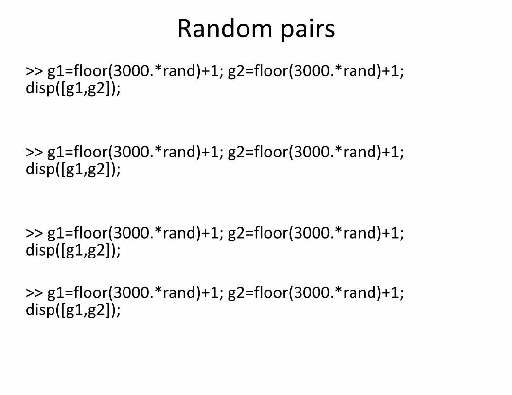
Random pairs>> g1=floor(3000.*rand)+1; g2=floor(3000.*rand)+1; disp([g1,g2]);

>> g1=floor(3000.*rand)+1; g2=floor(3000.*rand)+1; disp([g1,g2]);

>> g1=floor(3000.*rand)+1; g2=floor(3000.*rand)+1; disp([g1,g2]);

>> g1=floor(3000.*rand)+1; g2=floor(3000.*rand)+1; disp([g1,g2]);

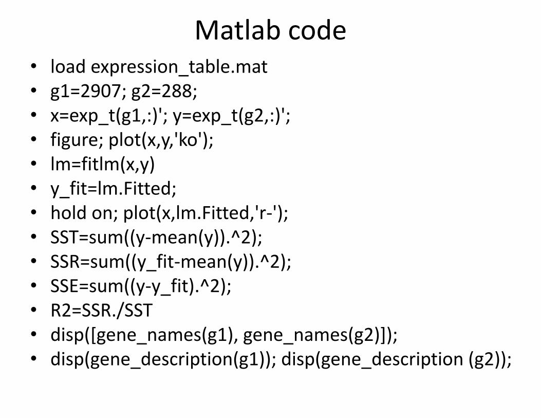
Matlab code• load expression_table.mat• g1=2907; g2=288;• x=exp_t(g1,:)'; y=exp_t(g2,:)';• figure; plot(x,y,'ko');• lm=fitlm(x,y)• y_fit=lm.Fitted;• hold on; plot(x,lm.Fitted,'r‐');• SST=sum((y‐mean(y)).^2);• SSR=sum((y_fit‐mean(y)).^2);• SSE=sum((y‐y_fit).^2);• R2=SSR./SST• disp([gene_names(g1), gene_names(g2)]);• disp(gene_description(g1)); disp(gene_description (g2));