Pulses in transmission lines

Physics 401, Fall 2017Eugene V. Colla

• Definition

• Distributed parameters network

• Pulses in transmission line

• Wave equation and wave propagation

• Reflections. Resistive load

• Thévenin's theorem

• Reflection. Non resistive load

• Appendix. Error propagation

9/18/2017 2Spring 2016

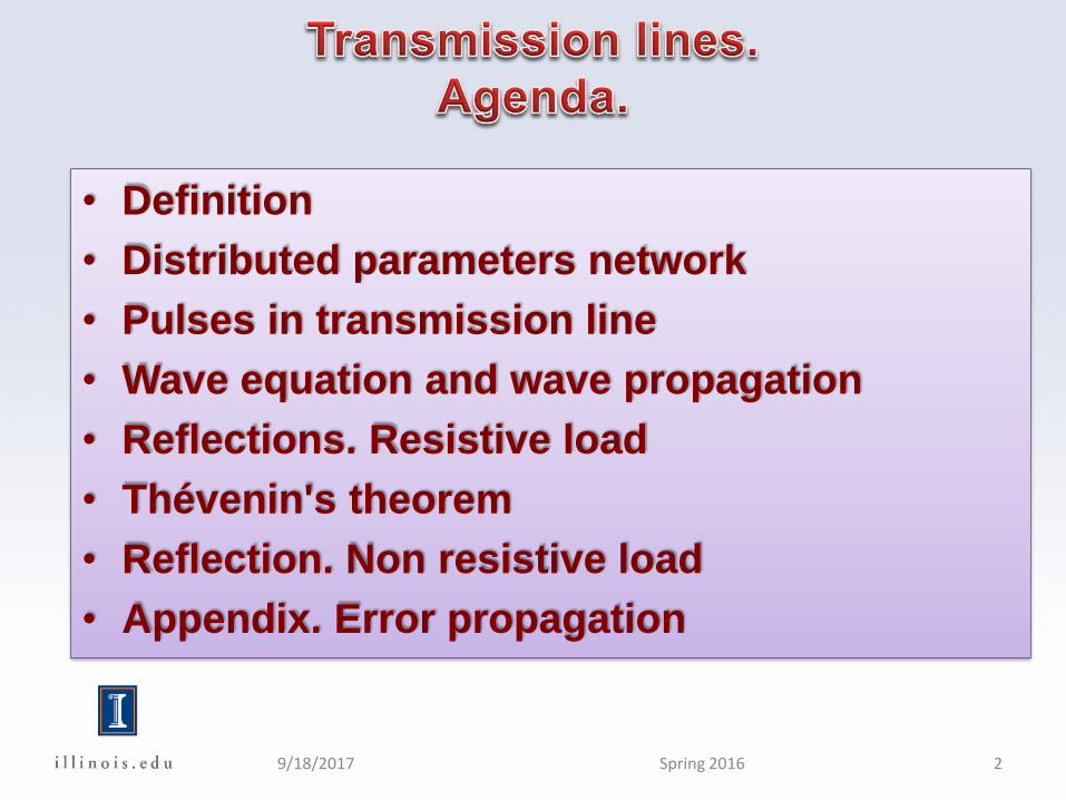
• Transmission line is a specialized cable

designed to carry alternating current of radio

frequency, that is, currents with a frequency

high enough that its wave nature must be

taken into account.

Courtesy Wikipedia

9/18/2017 3Spring 2016

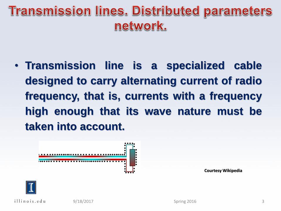
LiLi-1 Li+1

CiCi-1 Ci+1

Idealcase

Ci

Gi+1

LiRi Real situation

Simplified equalent

circuit

9/18/2017 4Spring 2016

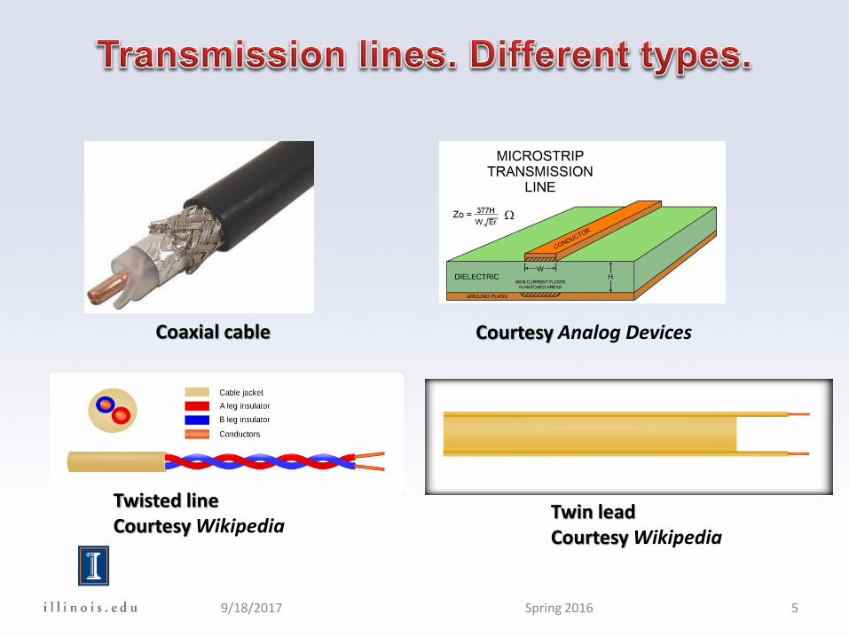
9/18/2017 5Spring 2016

Coaxial cable Courtesy Analog Devices

Twisted lineCourtesy Wikipedia

Twin leadCourtesy Wikipedia

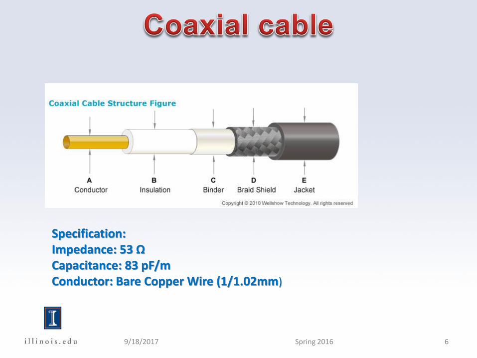
Specification:Impedance: 53 ΩCapacitance: 83 pF/mConductor: Bare Copper Wire (1/1.02mm)

9/18/2017 6Spring 2016

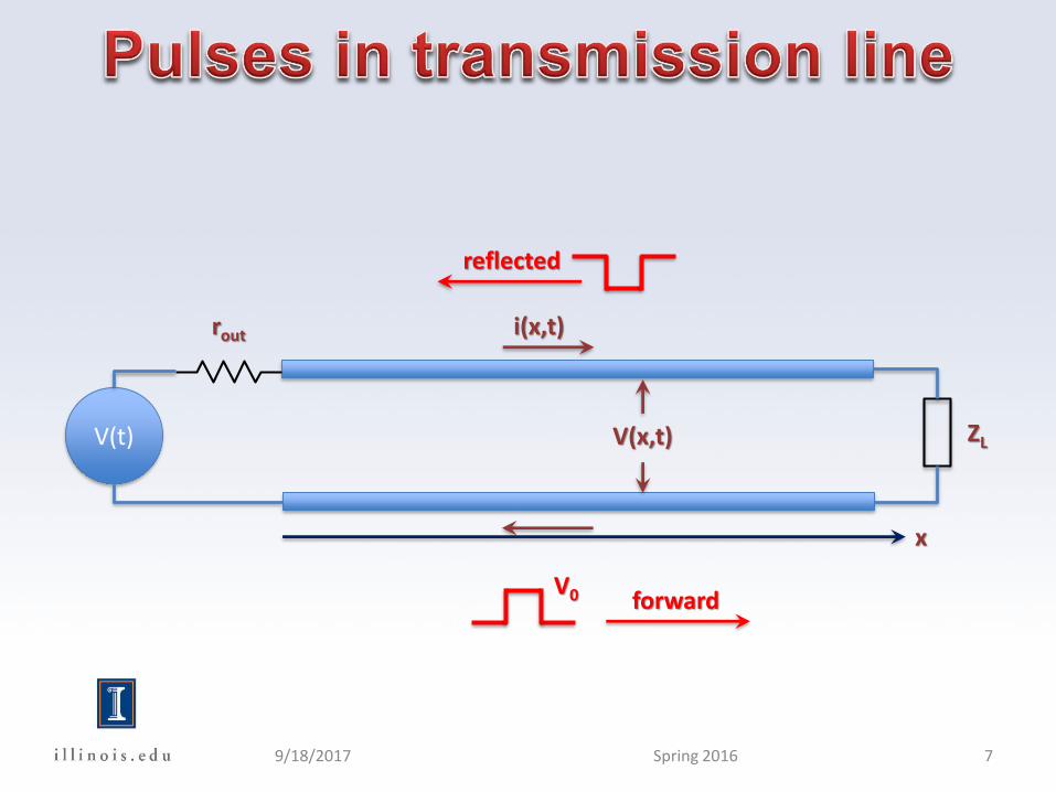
V(t) V(x,t)

x

ZL

rout i(x,t)

V0 forward

reflected

9/18/2017 7Spring 2016

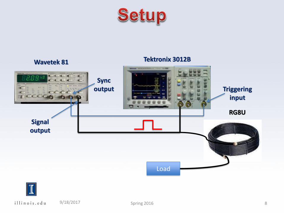
Load

RG8U

Wavetek 81 Tektronix 3012B

Triggering input

Sync output

Signal output

9/18/2017 8Spring 2016

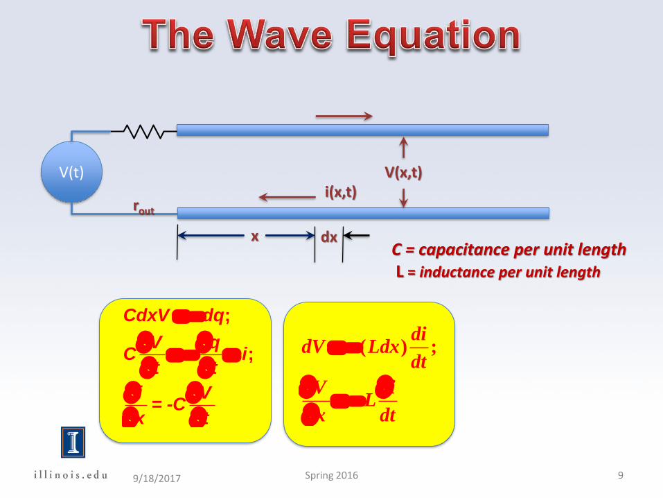
V(t) V(x,t)

x

rout

i(x,t)

dxC = capacitance per unit lengthL = inductance per unit length

;

;

CdxV dq

V qC i

t t

i V= -C

x t

( ) ;

didV Ldx

dt

V iL

x dt

9/18/2017 9Spring 2016

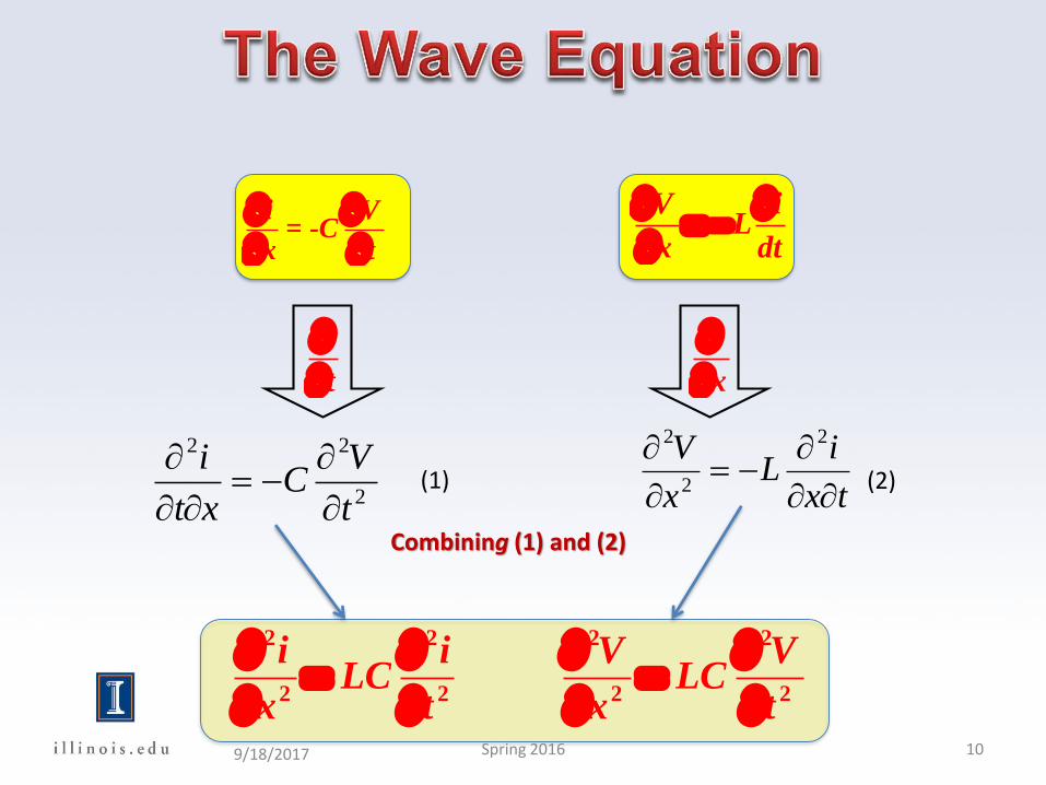
i V= -C

x t

V iL

x dt

t

x

tx

iL

x

V

2

2

2

2

22

t

VC

xt

i

(1) (2)

Combining (1) and (2)

2 2

2 2

V VLC

x t

2 2

2 2

i iLC

x t9/18/2017 10Spring 2016

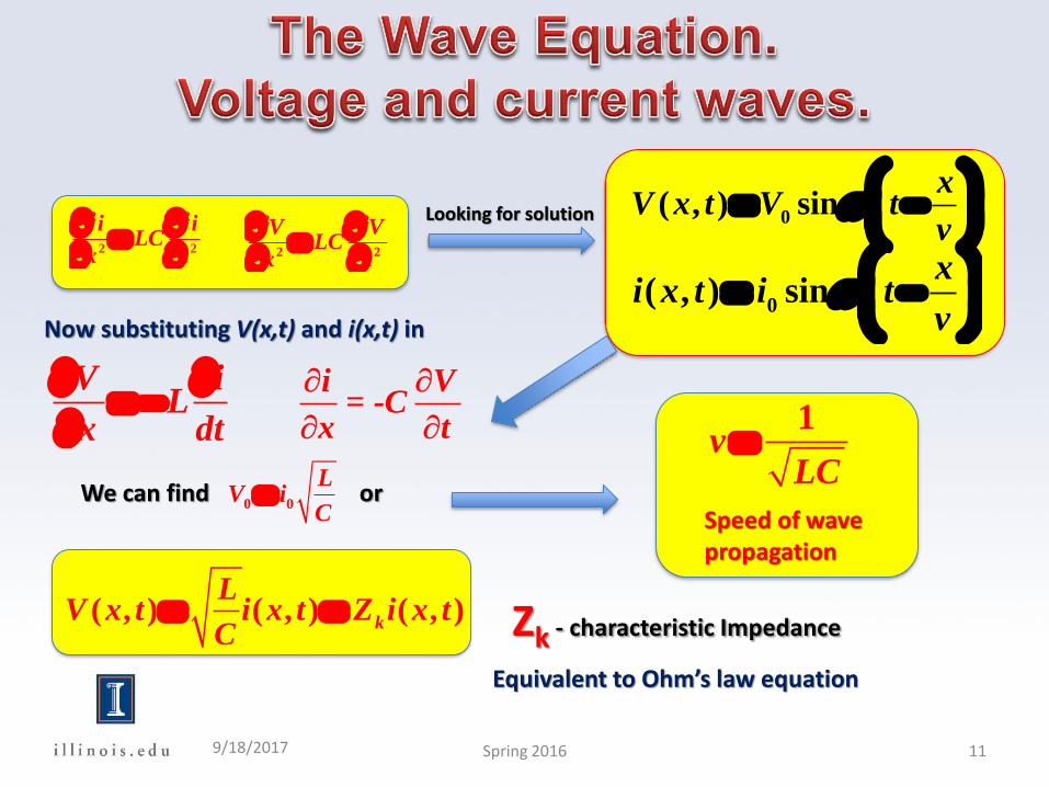
2 2

2 2

V VLC

x t

2 2

2 2

i iLC

x t

0( , ) sin

xV x t V t

v

0( , ) sin

xi x t i t

v

Looking for solution

1

vLC

Speed of wavepropagation

V iL

x dt

Now substituting V(x,t) and i(x,t) in

We can find or 0 0

LV i

C

( , ) ( , ) ( , ) k

LV x t i x t Z i x t

C Zk - characteristic Impedance

Equivalent to Ohm’s law equation

i V= -C

x t

9/18/2017 11Spring 2016

k

LZ =

C

C = capacitance per unit lengthL = inductance per unit length

Cross-section of the coaxial cable

Dd

0 r2πε ε

C=D

lnd

(F/m)

-12

0ε =8.854×10 (F/m)

er – dielectric permittivitymr-magnetic permeability ≈1

0 ln2

m m

r D

Ld

-7

0=4 ×10 (H/m)m

(H/m)

Finally for coaxial cable: 138

log ( )e

k

r

DZ Ohms

d

9/18/2017 12Spring 2016

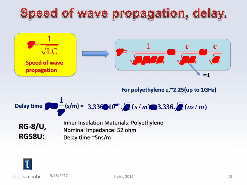
1

=LC

Speed of wavepropagation

1

=0 0

m m e e m e e

r r r r r

c c

Delay time (s/m) ≈

For polyethylene er~2.25(up to 1GHz)

1

9

3.336 10 ( / ) 3.336 ( / )e er r

s m ns m

RG-8/U, RG58U:

Inner Insulation Materials: Polyethylene Nominal Impedance: 52 ohm Delay time ~5ns/m

1

9/18/2017 13Spring 2016

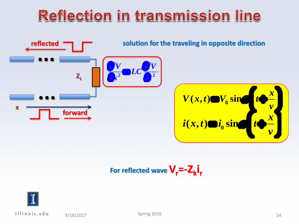
x

ZL

forward

reflected

...

...

2 2

2 2

V VLC

x t

solution for the traveling in opposite direction

For reflected wave Vr=-Zkir

0( , ) sin

xV x t V t

v

0( , ) sin

xi x t i t

v

9/18/2017 14Spring 2016

x

ZL

forward

reflected

...

...

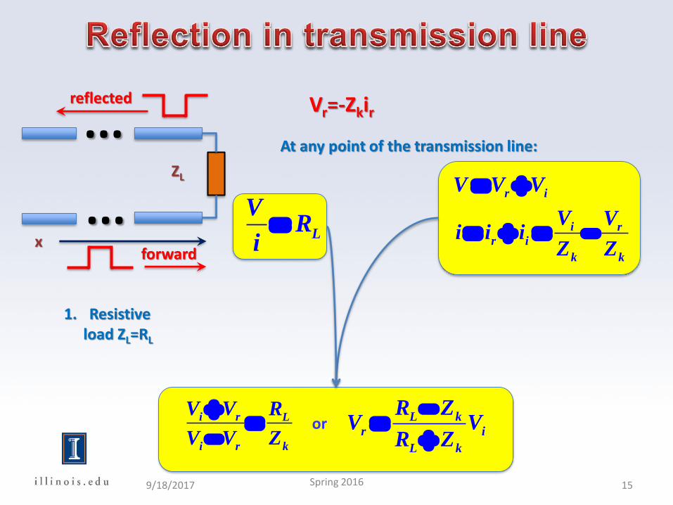
Vr=-Zkir

At any point of the transmission line:

r i

i r

r i

k k

V V V

V Vi i i

Z Z

1. Resistive load ZL=RL

L

VR

i

i r L

i r k

V V R

V V Z

or L k

r i

L k

R ZV V

R Z

9/18/2017 15Spring 2016

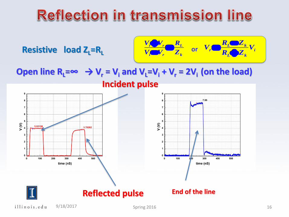
Resistive load ZL=RL

i r L

i r k

V V R

V V Z

orL k

r i

L k

R ZV V

R Z

Open line RL=∞ → Vr = Vi and VL=Vi + Vr = 2Vi (on the load)

Incident pulse

Reflected pulse End of the line

9/18/2017 16Spring 2016

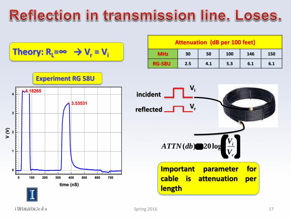
Theory: RL=∞ → Vr = Vi

Attenuation (dB per 100 feet)

MHz 30 50 100 146 150

RG-58U 2.5 4.1 5.3 6.1 6.1

Experiment RG 58U

Vi

Vr

incident

reflected

( ) 20log i

r

VATTN db

V

Important parameter forcable is attenuation perlength

9/18/2017 17Spring 2016

( ) 20log i

r

VATTN db

V

9/18/2017 18Spring 2016

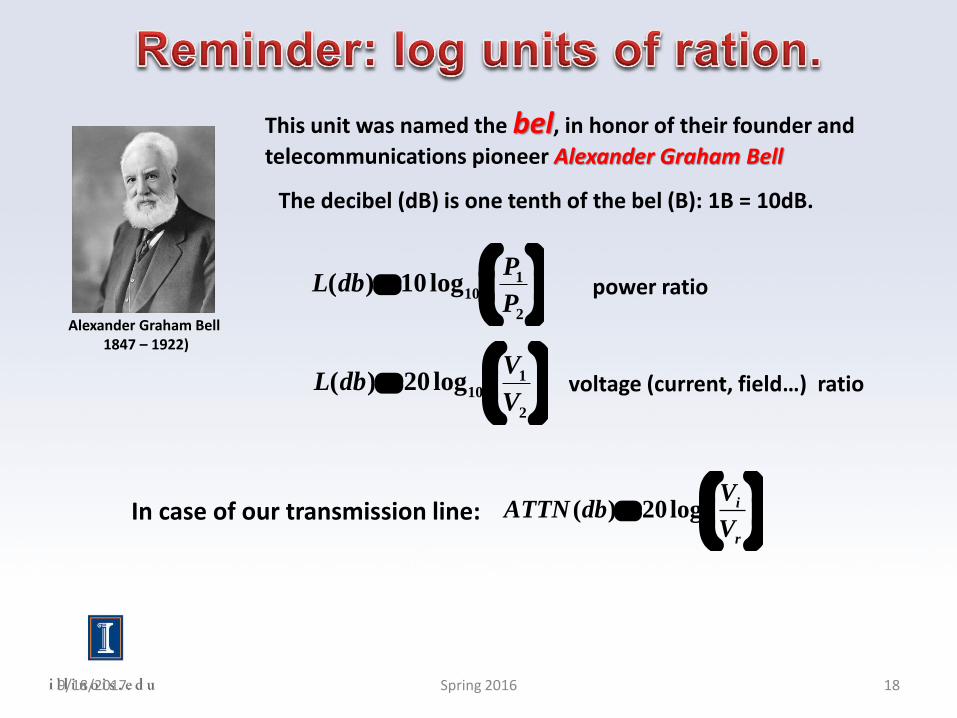
Alexander Graham Bell 1847 – 1922)

This unit was named the bel, in honor of their founder and

telecommunications pioneer Alexander Graham Bell

The decibel (dB) is one tenth of the bel (B): 1B = 10dB.

110

2

( ) 10 logP

L dbP

power ratio

110

2

( ) 20 logV

L dbV

voltage (current, field…) ratio

In case of our transmission line:

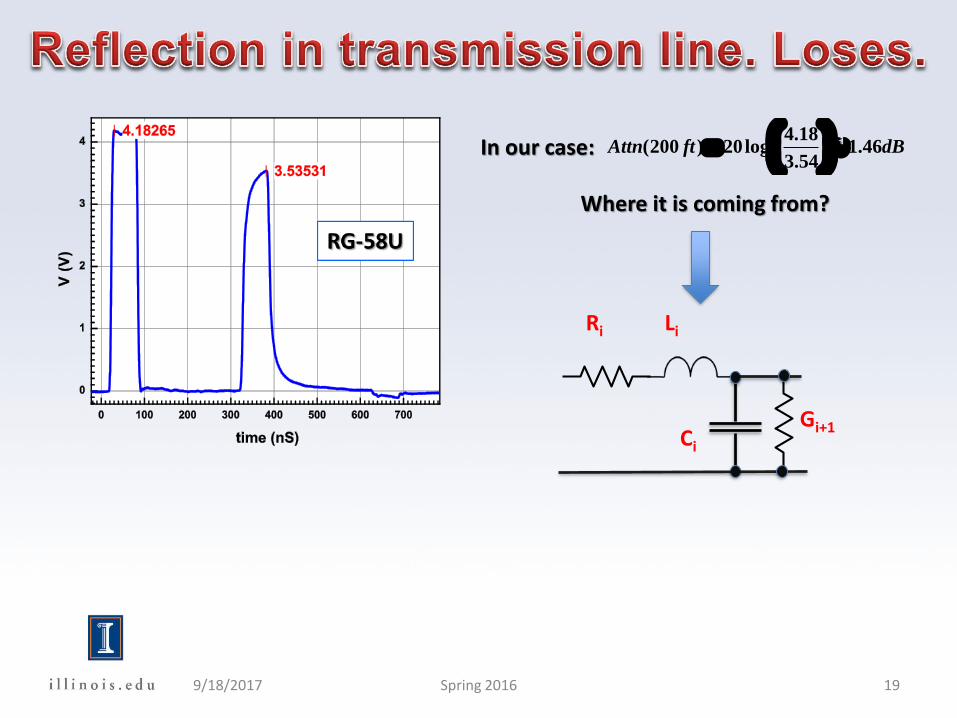
In our case:4.18

(200 ) 20log 1.463.54

Attn ft dB

Where it is coming from?

Ci

Gi+1

LiRi

9/18/2017 19Spring 2016

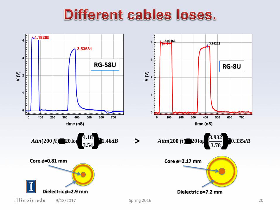
4.18(200 ) 20log 1.46

3.54Attn ft dB

3.932(200 ) 20log 0.335

3.78Attn ft dB

RG-58U RG-8U

Core ø=0.81 mm

Dielectric ø=2.9 mm

Core ø=2.17 mm

Dielectric ø=7.2 mm

>

9/18/2017 20Spring 2016

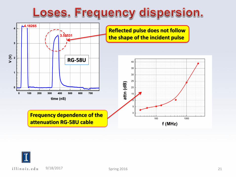
RG-58U

Reflected pulse does not follow the shape of the incident pulse

Frequency dependence of the attenuation RG-58U cable

9/18/2017 21Spring 2016

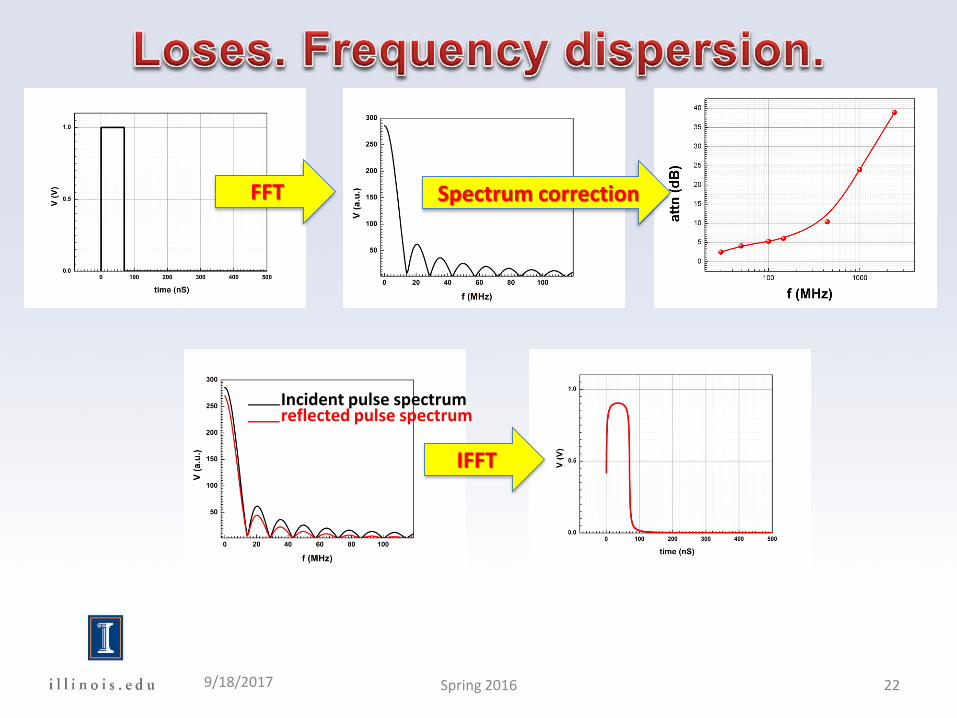
FFT Spectrum correction

Incident pulse spectrumreflected pulse spectrum

IFFT

9/18/2017 22Spring 2016

Resistive load ZL=RLi r L

i r k

V V R

V V Z

orL k

r i

L k

R ZV V

R Z

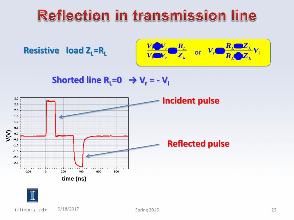
Shorted line RL=0 → Vr = - Vi

-200 0 200 400 600 800

-2.5

-2.0

-1.5

-1.0

-0.5

0.0

0.5

1.0

1.5

2.0

2.5

3.0

V(V

)

time (ns)

Incident pulse

Reflected pulse

9/18/2017 23Spring 2016

Resistive load ZL=RL i r L

i r k

V V R

V V Z

orL k

r i

L k

R ZV V

R Z

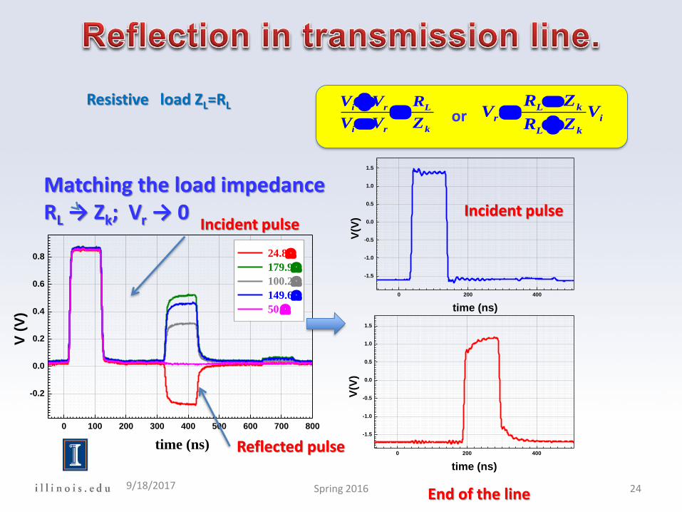
Matching the load impedance RL → Zk; Vr → 0

0 100 200 300 400 500 600 700 800

-0.2

0.0

0.2

0.4

0.6

0.8 24.8

179.9

100.2

149.6

50

time (ns)

V (

V)

0 200 400

-1.5

-1.0

-0.5

0.0

0.5

1.0

1.5

V(V

)

time (ns)

0 200 400

-1.5

-1.0

-0.5

0.0

0.5

1.0

1.5

V(V

)

time (ns)

Incident pulse

End of the line

Incident pulse

Reflected pulse

9/18/2017 24Spring 2016

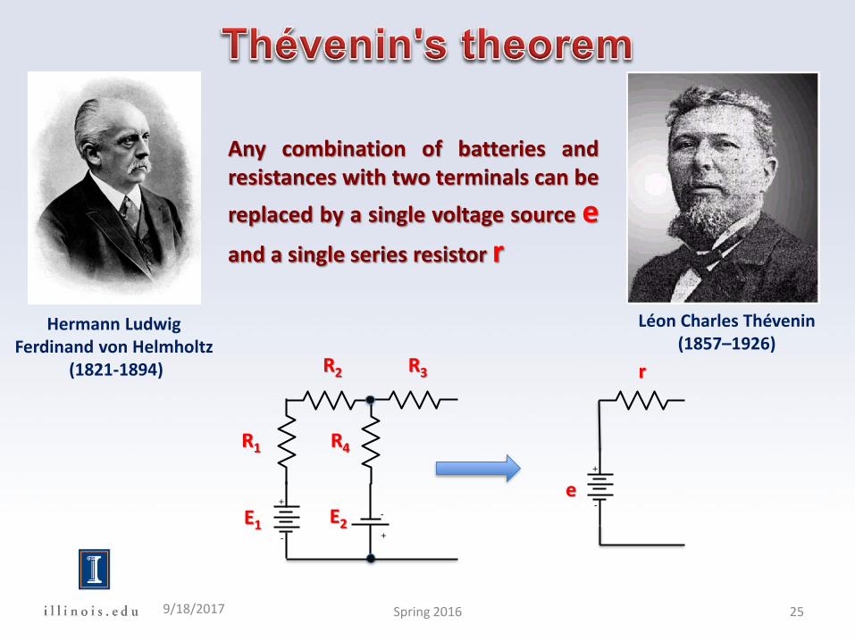
Léon Charles Thévenin(1857–1926)

Hermann Ludwig Ferdinand von Helmholtz

(1821-1894)

Any combination of batteries andresistances with two terminals can be

replaced by a single voltage source eand a single series resistor r

+

-

+

-

R1 R4

R2 R3

E1 E2

+

-

e

r

9/18/2017 25Spring 2016

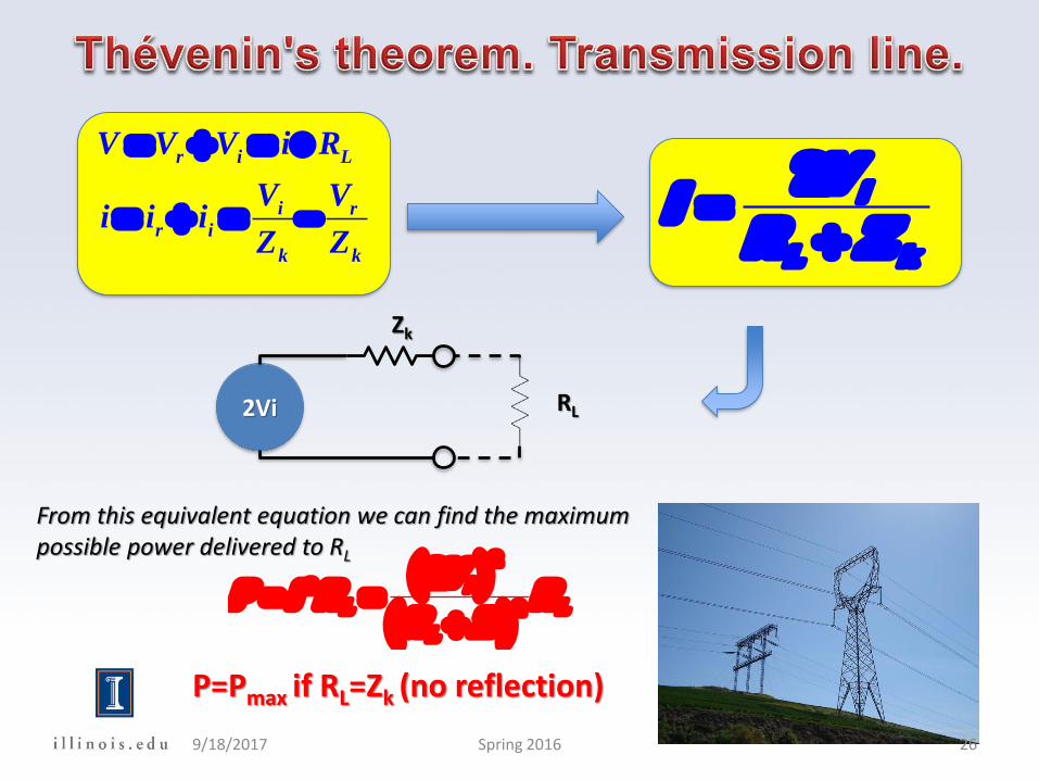
r i L

i r

r i

k k

V V V i R

V Vi i i

Z Z

i

L k

Vi

R Z

2

From this equivalent equation we can find the maximum possible power delivered to RL

i

L L

L

V

P i R R

R Z

2

2

2

2

P=Pmax if RL=Zk (no reflection)

2Vi

Zk

RL

9/18/2017 26Spring 2016

2Vi

Zk

RL

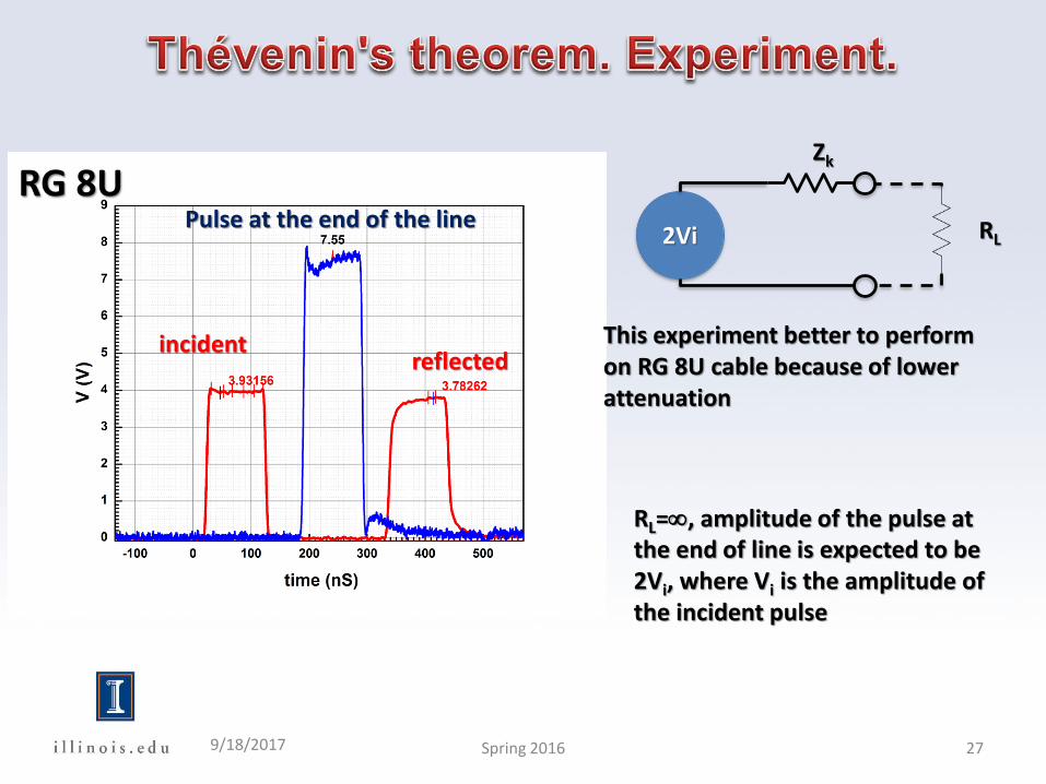
This experiment better to perform on RG 8U cable because of lower attenuation

RL=, amplitude of the pulse at the end of line is expected to be 2Vi, where Vi is the amplitude of the incident pulse

RG 8U

incidentreflected

Pulse at the end of the line

9/18/2017 27Spring 2016

i

L k

Vi

Z Z

2

V0

Zk

C

.

k

k

Z C

C nF

Z

3 2

9/18/2017 28Spring 2016

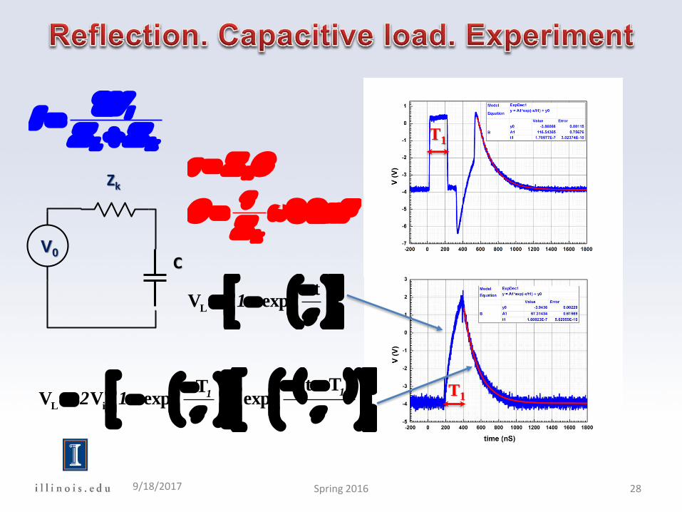
L

tV exp

1

L i

t TTV V exp exp

112 1

T1

T1

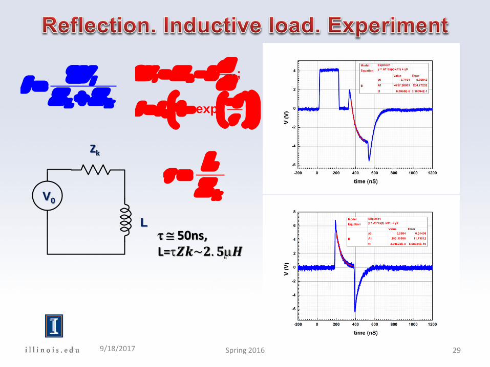
i

L k

Vi

Z Z

2

V0

L

Zk

;

exp ;

i k

diV iZ L

dt

ti i

0

2

1

k

L

Z

50ns, L=𝒁𝒌~𝟐. 𝟓m𝑯

9/18/2017 29Spring 2016

i

L k

Vi

Z Z

2

V0

L

Zk

;

exp ;

i k

diV iZ L

dt

ti i

0

2

1

k

L

Z

0

10

20

-10

0

10

20

-10 0 10 20 30 40 50 60-10

0

10

20

time

Vi

VL

Vr= VL - Vi

9/18/2017 30Spring 2016

9/18/2017 31Spring 2016

1. The reports should be uploaded to the proper folder and only to

the proper folder

L1_lab3_student1

Lab section Lab number Your name

2. Origin template for this week Lab:

\\engr-file-03\phyinst\APL Courses\PHYCS401\Common\Origin templates\Transmission line\Time trace.otp

9/18/2017 32Spring 2016

For example folder Frequency domain analys_L1 should used by students from L1 section only

I would recommend the file name style as:

You do not need to submit two copies in pdf and in MsWord formats

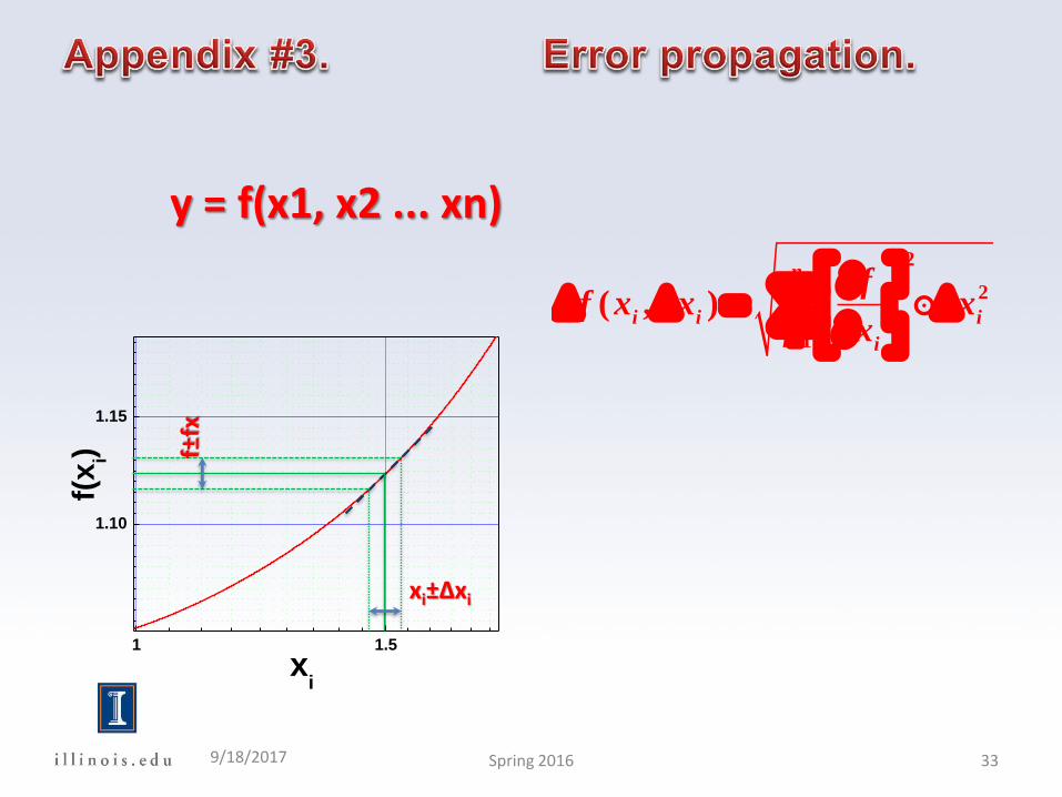
y = f(x1, x2 ... xn)2

2

1

( , )n

i i i

i i

ff x x x

x

1 1.5

1.10

1.15

xi

f(x

i)

xi±∆xi

f±fx

9/18/2017 33Spring 2016

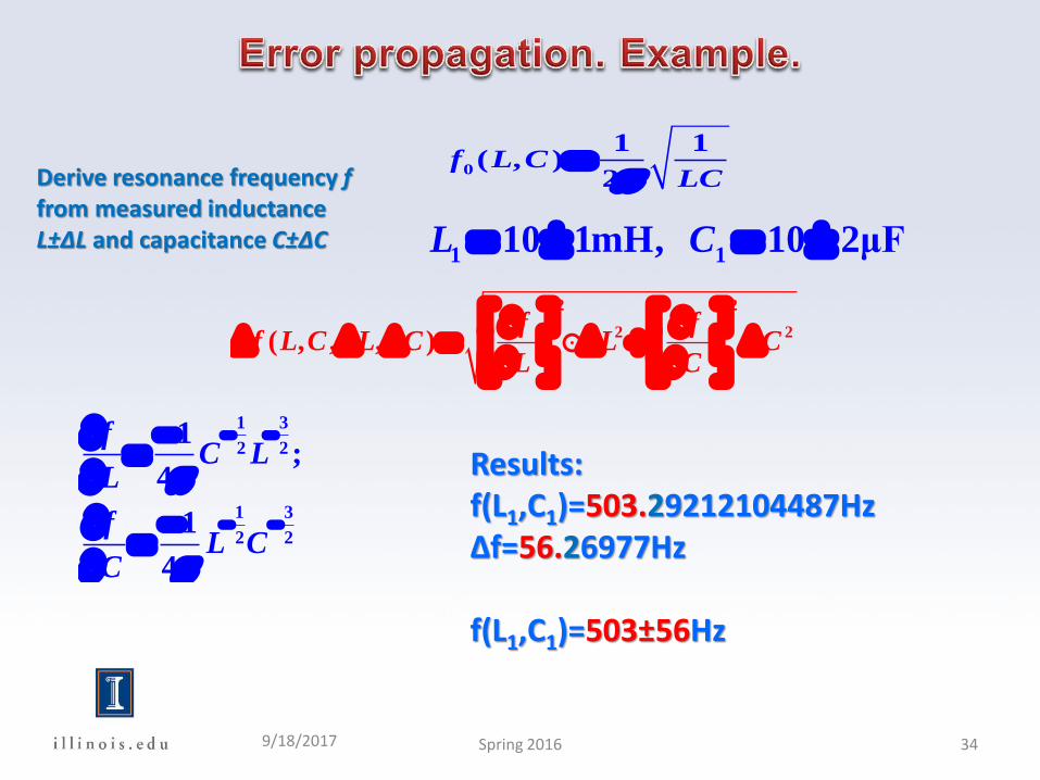
Derive resonance frequency ffrom measured inductanceL±∆L and capacitance C±∆C

0

1

1( , )

2

f L CLC

1 110 1mH, 10 2μFL C

2 2

2 2( , , , )

f ff L C L C L C

L C

1 3

2 2

1 3

2 2

1;

4

1

4

fC L

L

fL C

C

Results: f(L1,C1)=503.29212104487Hz∆f=56.26977Hz

f(L1,C1)=503±56Hz

9/18/2017 34Spring 2016

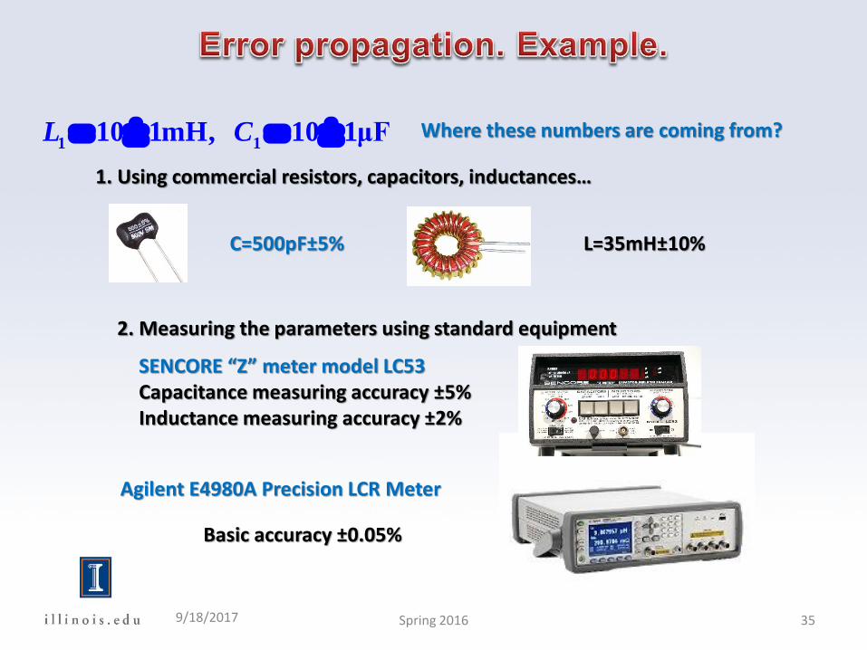
1 110 1mH, 10 1μFL C Where these numbers are coming from?

1. Using commercial resistors, capacitors, inductances…

C=500pF±5% L=35mH±10%

2. Measuring the parameters using standard equipment

SENCORE “Z” meter model LC53Capacitance measuring accuracy ±5%Inductance measuring accuracy ±2%

Basic accuracy ±0.05%

Agilent E4980A Precision LCR Meter

9/18/2017 35Spring 2016

9/18/2017 36Spring 2016

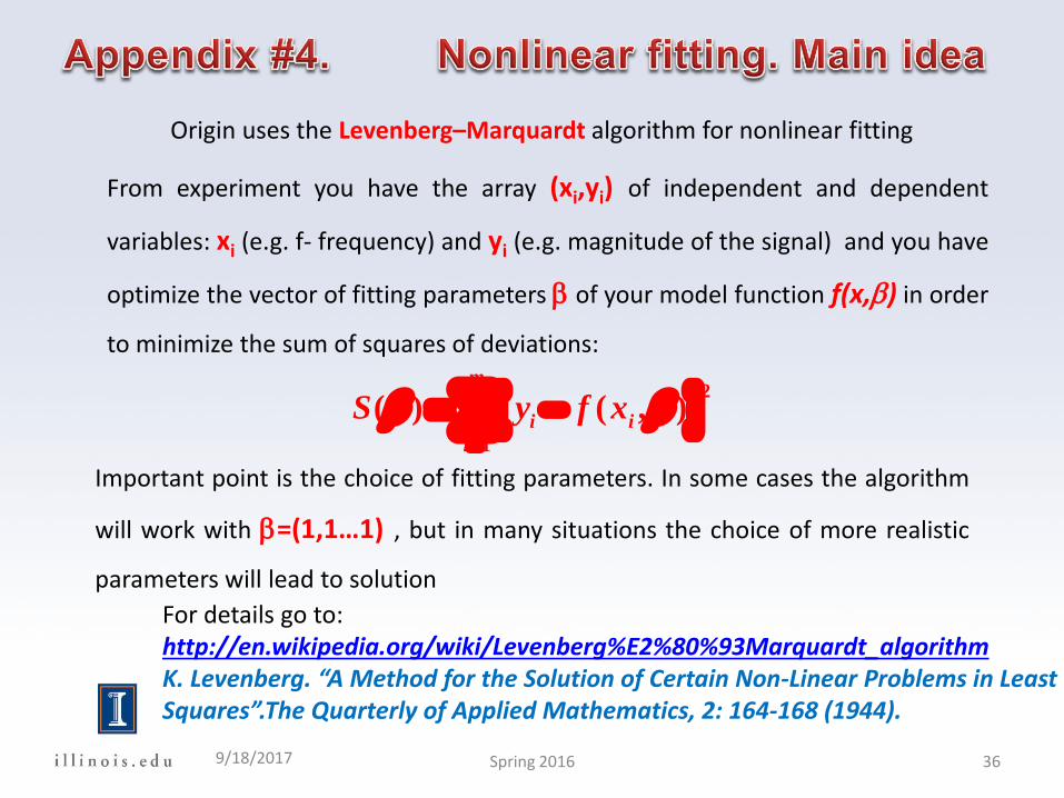
Origin uses the Levenberg–Marquardt algorithm for nonlinear fitting

From experiment you have the array (xi,yi) of independent and dependent

variables: xi (e.g. f- frequency) and yi (e.g. magnitude of the signal) and you have

optimize the vector of fitting parameters b of your model function f(x,b) in order

to minimize the sum of squares of deviations:

2

1

( ) ( , )m

i i

i

S y f xb b

Important point is the choice of fitting parameters. In some cases the algorithm

will work with b=(1,1…1) , but in many situations the choice of more realistic

parameters will lead to solution

For details go to: http://en.wikipedia.org/wiki/Levenberg%E2%80%93Marquardt_algorithmK. Levenberg. “A Method for the Solution of Certain Non-Linear Problems in Least Squares”.The Quarterly of Applied Mathematics, 2: 164-168 (1944).

9/18/2017 37Spring 2016

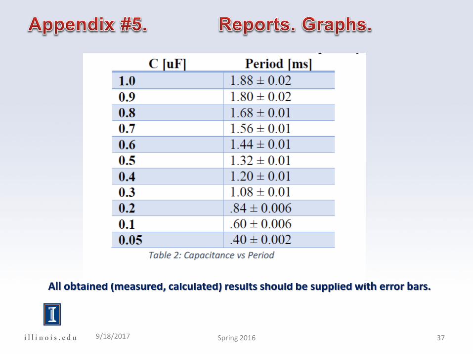
All obtained (measured, calculated) results should be supplied with error bars.

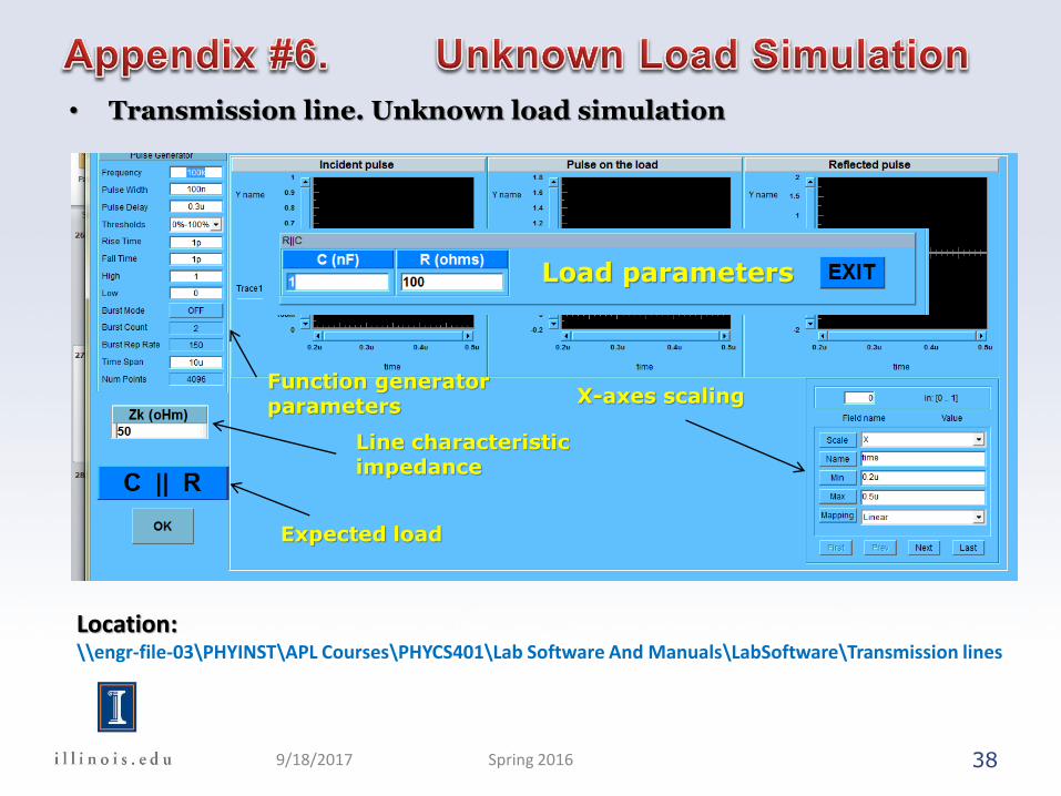
• Transmission line. Unknown load simulation

38

X-axes scalingFunction generator parameters

Line characteristic impedance

Expected load

Load parameters

Location:\\engr-file-03\PHYINST\APL Courses\PHYCS401\Lab Software And Manuals\LabSoftware\Transmission lines

9/18/2017 Spring 2016

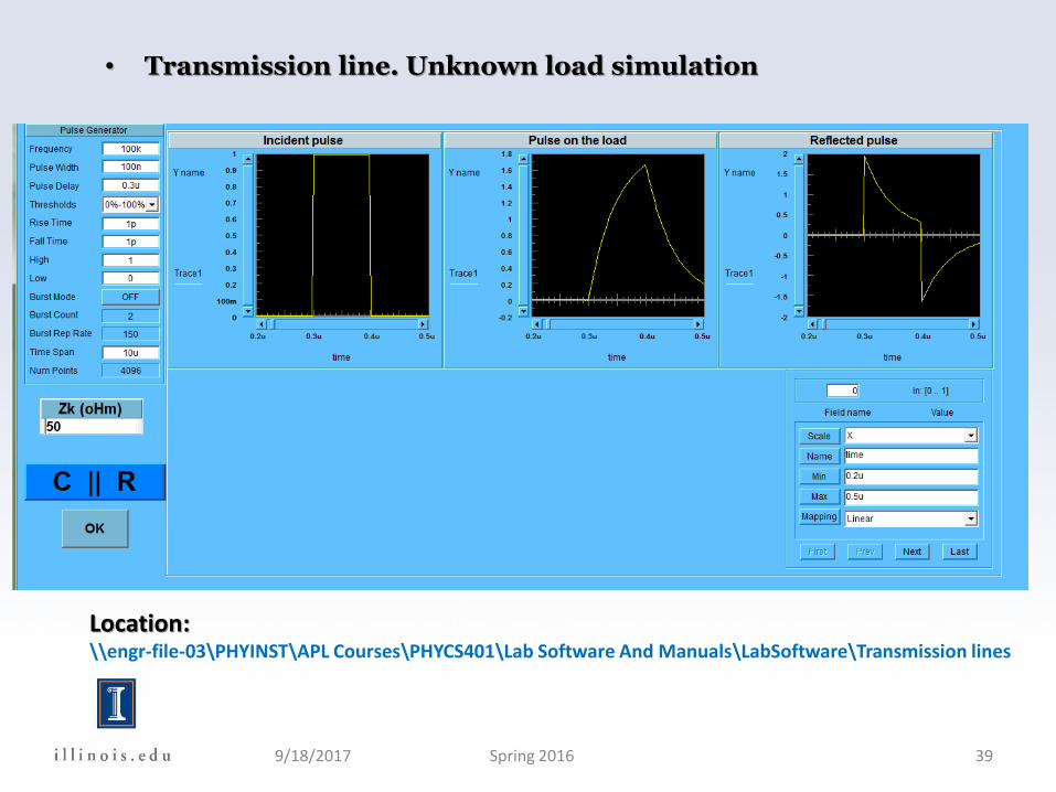
• Transmission line. Unknown load simulation

Location:\\engr-file-03\PHYINST\APL Courses\PHYCS401\Lab Software And Manuals\LabSoftware\Transmission lines

9/18/2017 Spring 2016 39