PHYSICAL REVIEW E 84, 016604 (2011)

Dissipative rogue waves: Extreme pulses generated by passively mode-locked lasers

J. M. Soto-Crespo,1 Ph. Grelu,2 and Nail Akhmediev3

1Instituto de Optica, CSIC, Serrano 121, E-28006 Madrid, Spain2Laboratoire Interdisciplinaire Carnot de Bourgogne, UMR 5209 CNRS, Universite de Bourgogne, 9 avenue A. Savary,

BP 47870, Dijon Cedex F-21078, France3Optical Sciences Group, Research School of Physics and Engineering, Institute of Advanced Studies,

Australian National University, Canberra, Australian Capital Territory 0200, Australia(Received 26 April 2011; published 18 July 2011)

We study numerically rogue waves in dissipative systems, taking as an example a unidirectional fiber laserin a nonstationary regime of operation. The choice of specific set of parameters allows the laser to generate achaotic sequence of pulses with a random distribution of peak amplitudes. The probability density function forthe intensity maxima has an elevated tail at higher intensities. We have found that the probability of producingextreme pulses in this setup is higher than in any other system considered so far.

DOI: 10.1103/PhysRevE.84.016604 PACS number(s): 05.45.Yv, 42.65.−k, 47.20.Ky

I. INTRODUCTION

The concept of rogue waves describes a unifying idea thatapplies to a number of extreme phenomena in hydrodynamics,optics, plasma physics, and other fields [1]. It has been studiedextensively in the case of ocean waves [2–5], as this is essentialfor reducing the travel risk for mariners. In recent years, thesestudies have extended to the areas of optics [6], capillarywaves [7], and even finance [8], thus enriching significantlythe original concept.

Until now, rogue waves were mostly studied in conservativesystems, with the nonlinear Schrodinger equation (NLSE)being the most popular model [2]. However, experience tellsus that rogue waves cannot appear without a sufficient energysupply. This seems to be a paradox. Indeed, how a conservativesystem that conserves energy can generate rogue waves, whichrequire a significant amount of external energy to be pumpedinto them?

The solution for this paradox is more or less simple. Inthe case of the NLSE, exact solutions to model rogue wavescontained a finite background. Thus, the energy supply forthe rogue waves is provided by the infinitely distributedcontinuous wave which carries an infinite amount of energy.For example, Peregrine solitons [9], which are consideredprototypes of rogue waves in the ocean [10] and in optics [11],are always located on a finite background. This background isnecessary as it serves as an unlimited energy supply for therogue waves whenever they appear. Generally speaking, thebackground is unstable and splits into a multiplicity of pulses.However, the unlimited amount of energy is still there becauseof the conservative nature of the model.

In the open ocean, the background is created by the windsover the water surface. Indeed, in most cases, rogue wavescannot appear in the quiet ocean. Stormy conditions are oneof the essential prerequisites for their generation. Transfer ofthe background energy into a single strong wave is the mainmechanism for generating rogue waves.

Incorporating the energy supply into the nonlinear waveequation instead of using a conservative system seems tobe a natural way to further improve the model. Thus,generalizing the model and using a dissipative system with

an external energy supply from the very beginning may beuseful in considering rogue waves. The first attempts of suchgeneralization have already been done. Montina et al. [12]studied non-Gaussian statistics and extreme waves in aunidirectional optical oscillator pumped with an external lightbeam. Self-splitting of the beam into small-scale, stronglyfocused “optical needles” created conditions in which someof these filaments contained significantly more energy thanthe average, thus generating a specific form of rogue waves.

In the present work, we use a model different from thatin [12]. Namely, we consider high-intensity waves in thetemporal domain rather than in space. Our system is definedby a set of equations that describes an optical cavity withgain and loss. In this model, we studied the optical fieldcreated when gain is high enough to generate a chaoticsequence of a multiplicity of pulses inside the cavity. Thissequence of pulses with chaotically distributed amplitudes isin continuous interaction and may form pulses with amplitudessignificantly higher than the average. The pulses with thelargest amplitude can be considered rogue waves generated thisway. We confirmed numerically that their statistics are indeeddifferent from Gaussian. The probability distribution functionhas a long tail corresponding to high-amplitude waves, whichis a direct indication of the presence of rogue waves in thesystem.

II. THE MODEL

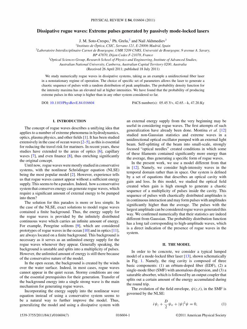
In order to be concrete, we consider a typical lumpedmodel of a mode-locked fiber laser [13], shown schematicallyin Fig. 1. Namely, the ring cavity is composed of threebasic components: (1) an erbium-doped fiber (EDF), (2) asingle-mode fiber (SMF) with anomalous dispersion, and (3) asaturable absorber, which is followed by an output coupler thatsplits out a certain amount of the energy accumulated duringthe round trip.

The evolution of the field envelope, ψ(z,t), in the SMF isgoverned by the NLSE:

iψz + D

2ψtt + |ψ |2ψ = 0, (1)

016604-11539-3755/2011/84(1)/016604(7) ©2011 American Physical Society

J. M. SOTO-CRESPO, PH. GRELU, AND NAIL AKHMEDIEV PHYSICAL REVIEW E 84, 016604 (2011)

EDF

SM F

0.5dB

SA

OCIout

FIG. 1. (Color online) Model of the fiber laser used in oursimulations. Notations are as follows: SMF, single mode fiber; SA,saturable absorber; OC, output coupler; and EDF, erbium-doped fiber.

where D is the dispersion parameter, z is the propagationdistance, and t is the time in a frame of reference moving withthe group velocity, all in normalized dimensionless units.

Pulse propagation in the EDF is modeled by

iψz + D2

2ψtt + �2|ψ |2ψ = igo

1 + Q/Qsat(ψ + β2ψtt ), (2)

where the total energy Q is

Q =∫ ∞

−∞|ψ |2dt,

Qsat is the parameter representing the saturation energy, go isthe small signal gain, and β2 represents the spectral width ofthe gain. �2 is the ratio between the nonlinear coefficients inthe EDF and SMF. More precisely, it corresponds to the ratiobetween the effective mode areas of the EDF and SMF, whenboth fibers are made of the same glass material, for example,silica.

The instantaneous saturable absorber (SA) is modeled bythe following transfer function:

T = To + �TI (t)

Isat + I (t), (3)

where I (t) = |ψ(t)|2, To is the transmission level at lowintensities of the optical field, �T is the transmission contrast,and Isat is the saturation intensity. The output coupler ischaracterized by the transmission coefficient Tr . The latteris the coefficient representing power transfer between the twosections of the cavity. A typical 0.5-dB coupling loss is addedat the EDF-SMF junction.

The values of the parameters introduced with this modeldefine the mode of operation of the laser system. We canchoose the parameters in such a way that the laser operates inone of the following modes: (1) it is a continuous wave (CW)regime, (2) it generates a single stable, stationary pulse everyround trip, (3) it generates a periodically oscillating pulse withthe period equal to N round trips, (4) it generates several pulsesper round trip, or (5) it generates a chaotic field.

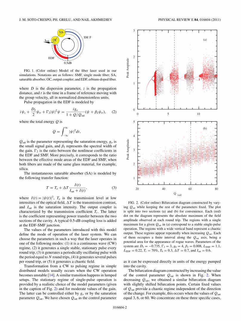
Transformation from a CW to pulsing regime in simpledistributed models usually occurs when the CW operationbecomes unstable [14]. A similar transition happens in lumpedsetups. The stationary regime of single-pulse operation isprovided by a realistic choice of the model parameters (givenin the caption of Fig. 2) and for moderate values of the gain.The latter can be controlled either by go or by the saturationparameter Qsat. We have chosen Qsat as the control parameter

0 5 100

1

2

3

(a)

(b)Pe

ak A

mpi

tude

20 40 60 80

1

2

3

4

5

Q sat

Peak

Am

plitu

de

FIG. 2. (Color online) Bifurcation diagram constructed by vary-ing Qsat while keeping the rest of the parameters fixed. The plotis split into two sections (a) and (b) for convenience. Each (red)dot on the diagram represents the absolute maximum of the fieldamplitude observed at each round trip. The regions with a singlemaximum for a given Qsat in (a) correspond to a stable single-pulseoperation. The regions with a wide vertical band represent a chaoticoutput. These regions appear repeatedly when increasing Qsat. Eachof them occupies a finite interval along the Qsat axis, being apotential area for the appearance of rogue waves. Parameters of thesystem are D2 = −0.735, �2 = 3, g0 = 4, β2 = 0.008, LSMF = 1.1,LEDF = 0.22, Tr = 70%, T0 = 0.3, �T = 0.7, and Isat = 0.6.

as it can be expressed directly in units of the energy pumpedinto the cavity.

The bifurcation diagram constructed by increasing the valueof the control parameter Qsat is shown in Fig. 2. Whendecreasing Qsat, we obtained a similar bifurcation diagramwith slightly shifted bifurcation points. Certain fixed valuesof Qsat provide a chaotic regime independent of the directionof the change. For example, this occurs when the values of Qsat

equal 3, 6, or 60. We concentrate on these three specific cases,

016604-2

DISSIPATIVE ROGUE WAVES: EXTREME PULSES . . . PHYSICAL REVIEW E 84, 016604 (2011)

−20 0 20 0

50

100

N

0

2

4

t

|ψ(t

,N)|

2

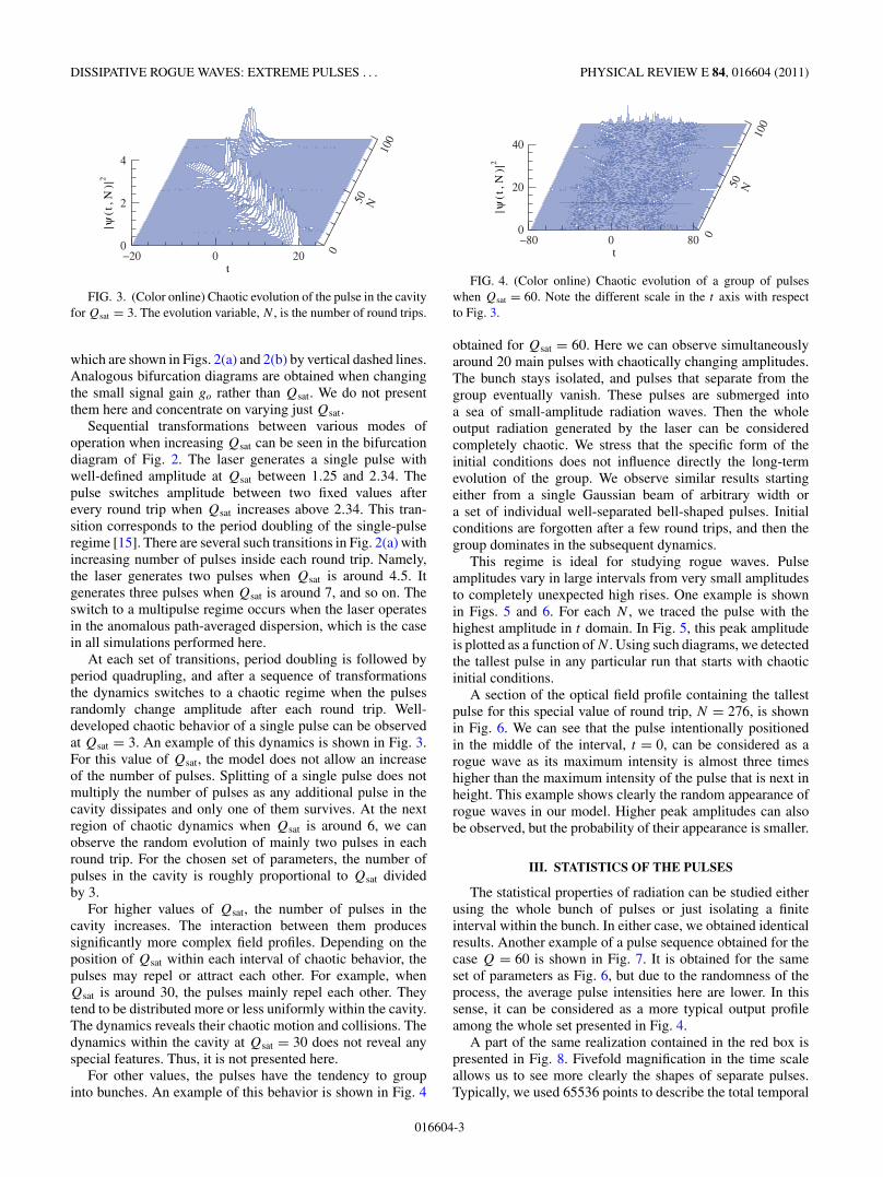
FIG. 3. (Color online) Chaotic evolution of the pulse in the cavityfor Qsat = 3. The evolution variable, N , is the number of round trips.

which are shown in Figs. 2(a) and 2(b) by vertical dashed lines.Analogous bifurcation diagrams are obtained when changingthe small signal gain go rather than Qsat. We do not presentthem here and concentrate on varying just Qsat.

Sequential transformations between various modes ofoperation when increasing Qsat can be seen in the bifurcationdiagram of Fig. 2. The laser generates a single pulse withwell-defined amplitude at Qsat between 1.25 and 2.34. Thepulse switches amplitude between two fixed values afterevery round trip when Qsat increases above 2.34. This tran-sition corresponds to the period doubling of the single-pulseregime [15]. There are several such transitions in Fig. 2(a) withincreasing number of pulses inside each round trip. Namely,the laser generates two pulses when Qsat is around 4.5. Itgenerates three pulses when Qsat is around 7, and so on. Theswitch to a multipulse regime occurs when the laser operatesin the anomalous path-averaged dispersion, which is the casein all simulations performed here.

At each set of transitions, period doubling is followed byperiod quadrupling, and after a sequence of transformationsthe dynamics switches to a chaotic regime when the pulsesrandomly change amplitude after each round trip. Well-developed chaotic behavior of a single pulse can be observedat Qsat = 3. An example of this dynamics is shown in Fig. 3.For this value of Qsat, the model does not allow an increaseof the number of pulses. Splitting of a single pulse does notmultiply the number of pulses as any additional pulse in thecavity dissipates and only one of them survives. At the nextregion of chaotic dynamics when Qsat is around 6, we canobserve the random evolution of mainly two pulses in eachround trip. For the chosen set of parameters, the number ofpulses in the cavity is roughly proportional to Qsat dividedby 3.

For higher values of Qsat, the number of pulses in thecavity increases. The interaction between them producessignificantly more complex field profiles. Depending on theposition of Qsat within each interval of chaotic behavior, thepulses may repel or attract each other. For example, whenQsat is around 30, the pulses mainly repel each other. Theytend to be distributed more or less uniformly within the cavity.The dynamics reveals their chaotic motion and collisions. Thedynamics within the cavity at Qsat = 30 does not reveal anyspecial features. Thus, it is not presented here.

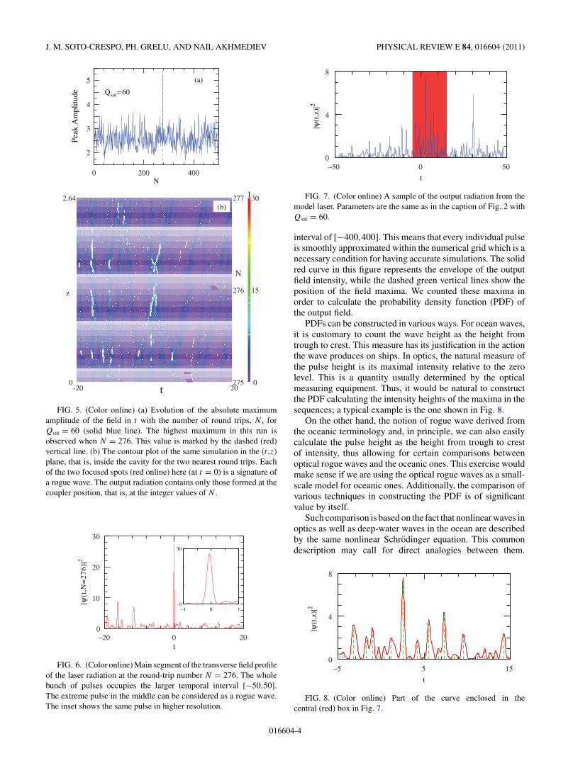
For other values, the pulses have the tendency to groupinto bunches. An example of this behavior is shown in Fig. 4

−80 0 80 0

50

100

N

0

20

40

t

|ψ(t

,N)|

2

FIG. 4. (Color online) Chaotic evolution of a group of pulseswhen Qsat = 60. Note the different scale in the t axis with respectto Fig. 3.

obtained for Qsat = 60. Here we can observe simultaneouslyaround 20 main pulses with chaotically changing amplitudes.The bunch stays isolated, and pulses that separate from thegroup eventually vanish. These pulses are submerged intoa sea of small-amplitude radiation waves. Then the wholeoutput radiation generated by the laser can be consideredcompletely chaotic. We stress that the specific form of theinitial conditions does not influence directly the long-termevolution of the group. We observe similar results startingeither from a single Gaussian beam of arbitrary width ora set of individual well-separated bell-shaped pulses. Initialconditions are forgotten after a few round trips, and then thegroup dominates in the subsequent dynamics.

This regime is ideal for studying rogue waves. Pulseamplitudes vary in large intervals from very small amplitudesto completely unexpected high rises. One example is shownin Figs. 5 and 6. For each N , we traced the pulse with thehighest amplitude in t domain. In Fig. 5, this peak amplitudeis plotted as a function of N . Using such diagrams, we detectedthe tallest pulse in any particular run that starts with chaoticinitial conditions.

A section of the optical field profile containing the tallestpulse for this special value of round trip, N = 276, is shownin Fig. 6. We can see that the pulse intentionally positionedin the middle of the interval, t = 0, can be considered as arogue wave as its maximum intensity is almost three timeshigher than the maximum intensity of the pulse that is next inheight. This example shows clearly the random appearance ofrogue waves in our model. Higher peak amplitudes can alsobe observed, but the probability of their appearance is smaller.

III. STATISTICS OF THE PULSES

The statistical properties of radiation can be studied eitherusing the whole bunch of pulses or just isolating a finiteinterval within the bunch. In either case, we obtained identicalresults. Another example of a pulse sequence obtained for thecase Q = 60 is shown in Fig. 7. It is obtained for the sameset of parameters as Fig. 6, but due to the randomness of theprocess, the average pulse intensities here are lower. In thissense, it can be considered as a more typical output profileamong the whole set presented in Fig. 4.

A part of the same realization contained in the red box ispresented in Fig. 8. Fivefold magnification in the time scaleallows us to see more clearly the shapes of separate pulses.Typically, we used 65536 points to describe the total temporal

016604-3

J. M. SOTO-CRESPO, PH. GRELU, AND NAIL AKHMEDIEV PHYSICAL REVIEW E 84, 016604 (2011)

t-20 200

2.64

275

277

276

0

30

15z

N

I

(b)

0 200 400

2

3

4

5Qsat=60

(a)

N

Peak

Am

plitu

de

FIG. 5. (Color online) (a) Evolution of the absolute maximumamplitude of the field in t with the number of round trips, N , forQsat = 60 (solid blue line). The highest maximum in this run isobserved when N = 276. This value is marked by the dashed (red)vertical line. (b) The contour plot of the same simulation in the (t,z)plane, that is, inside the cavity for the two nearest round trips. Eachof the two focused spots (red online) here (at t = 0) is a signature ofa rogue wave. The output radiation contains only those formed at thecoupler position, that is, at the integer values of N .

−20 0 200

10

20

30

t

|ψ(t

,N=

276)

|2

−1 0 10

30

FIG. 6. (Color online) Main segment of the transverse field profileof the laser radiation at the round-trip number N = 276. The wholebunch of pulses occupies the larger temporal interval [−50,50].The extreme pulse in the middle can be considered as a rogue wave.The inset shows the same pulse in higher resolution.

−50 0 500

4

8

t

|ψ(t

,z)|2

FIG. 7. (Color online) A sample of the output radiation from themodel laser. Parameters are the same as in the caption of Fig. 2 withQsat = 60.

interval of [−400,400]. This means that every individual pulseis smoothly approximated within the numerical grid which is anecessary condition for having accurate simulations. The solidred curve in this figure represents the envelope of the outputfield intensity, while the dashed green vertical lines show theposition of the field maxima. We counted these maxima inorder to calculate the probability density function (PDF) ofthe output field.

PDFs can be constructed in various ways. For ocean waves,it is customary to count the wave height as the height fromtrough to crest. This measure has its justification in the actionthe wave produces on ships. In optics, the natural measure ofthe pulse height is its maximal intensity relative to the zerolevel. This is a quantity usually determined by the opticalmeasuring equipment. Thus, it would be natural to constructthe PDF calculating the intensity heights of the maxima in thesequences; a typical example is the one shown in Fig. 8.

On the other hand, the notion of rogue wave derived fromthe oceanic terminology and, in principle, we can also easilycalculate the pulse height as the height from trough to crestof intensity, thus allowing for certain comparisons betweenoptical rogue waves and the oceanic ones. This exercise wouldmake sense if we are using the optical rogue waves as a small-scale model for oceanic ones. Additionally, the comparison ofvarious techniques in constructing the PDF is of significantvalue by itself.

Such comparison is based on the fact that nonlinear waves inoptics as well as deep-water waves in the ocean are describedby the same nonlinear Schrodinger equation. This commondescription may call for direct analogies between them.

−5 5 150

4

8

t

|ψ(t

,z)|2

FIG. 8. (Color online) Part of the curve enclosed in thecentral (red) box in Fig. 7.

016604-4

DISSIPATIVE ROGUE WAVES: EXTREME PULSES . . . PHYSICAL REVIEW E 84, 016604 (2011)

However, even if the equation is the same, the measurablequantities are different. Namely, in optics, we measure theintensity, that is, the square modulus of the amplitude ofthe envelope of the carrier wave, which is a complex field.In the case of deep-water waves, the carrier wave is a realfunction. A measurable quantity is the real part of the envelopemultiplied by the carrier wave. This difference leads to asignificant distinction between the two types of waves. Directcomparisons should be done with care.

Although for conventional laser applications, people havebeen mostly interested in low-noise CW radiation on the onehand and stable single-pulse mode locking on the other hand,there is presently a growing interest in studying chaotic laserradiation. A decade after the intensive studies of the statisticalproperties of transverse laser modes [16], research has focusedon the statistical properties of single transverse-mode laseremitters. Indeed, chaotic quasi-CW oscillators could be ap-plied in optical cryptography for secure communications [17],whereas noiselike, wide-band laser pulses can be useful forlow-coherence reflectometry [18]. However, the generation ofa truly chaotic field in the temporal domain is still largelymysterious. Although pulse generation in mode-locked lasersis presently well understood, the recent focus on excitabledynamics within the multiple-pulse quasi-mode-locked regimestimulates further interest in exploration of this type ofsystems [19].

Generally, the statistics of laser radiation is measured asthe second factorial moment [20]. Roughly speaking, the mainvalue of interest is the intensity distribution of the outputradiation. Depending on the model, this distribution can lookGaussian [20] or can be a more complicated function of theintensity [21]. When studying rogue waves, we are dealingwith the distribution of the maxima of radiation rather thanradiation at every point. We expect that the density of maximashould be different from the density of probability at everypoint of radiation.

IV. PROBABILITY DENSITY FUNCTION

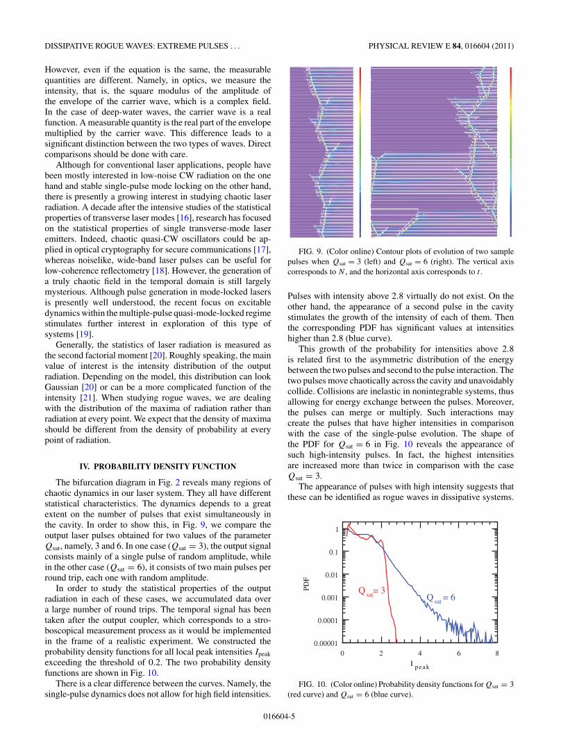
The bifurcation diagram in Fig. 2 reveals many regions ofchaotic dynamics in our laser system. They all have differentstatistical characteristics. The dynamics depends to a greatextent on the number of pulses that exist simultaneously inthe cavity. In order to show this, in Fig. 9, we compare theoutput laser pulses obtained for two values of the parameterQsat, namely, 3 and 6. In one case (Qsat = 3), the output signalconsists mainly of a single pulse of random amplitude, whilein the other case (Qsat = 6), it consists of two main pulses perround trip, each one with random amplitude.

In order to study the statistical properties of the outputradiation in each of these cases, we accumulated data overa large number of round trips. The temporal signal has beentaken after the output coupler, which corresponds to a stro-boscopical measurement process as it would be implementedin the frame of a realistic experiment. We constructed theprobability density functions for all local peak intensities Ipeak

exceeding the threshold of 0.2. The two probability densityfunctions are shown in Fig. 10.

There is a clear difference between the curves. Namely, thesingle-pulse dynamics does not allow for high field intensities.

FIG. 9. (Color online) Contour plots of evolution of two samplepulses when Qsat = 3 (left) and Qsat = 6 (right). The vertical axiscorresponds to N , and the horizontal axis corresponds to t .

Pulses with intensity above 2.8 virtually do not exist. On theother hand, the appearance of a second pulse in the cavitystimulates the growth of the intensity of each of them. Thenthe corresponding PDF has significant values at intensitieshigher than 2.8 (blue curve).

This growth of the probability for intensities above 2.8is related first to the asymmetric distribution of the energybetween the two pulses and second to the pulse interaction. Thetwo pulses move chaotically across the cavity and unavoidablycollide. Collisions are inelastic in nonintegrable systems, thusallowing for energy exchange between the pulses. Moreover,the pulses can merge or multiply. Such interactions maycreate the pulses that have higher intensities in comparisonwith the case of the single-pulse evolution. The shape ofthe PDF for Qsat = 6 in Fig. 10 reveals the appearance ofsuch high-intensity pulses. In fact, the highest intensitiesare increased more than twice in comparison with the caseQsat = 3.

The appearance of pulses with high intensity suggests thatthese can be identified as rogue waves in dissipative systems.

0 2 4 6 80.00001

0.0001

0.001

0.01

0.1

1

Qsat= 3Qsat = 6

I p e a k

PDF

FIG. 10. (Color online) Probability density functions for Qsat = 3(red curve) and Qsat = 6 (blue curve).

016604-5

J. M. SOTO-CRESPO, PH. GRELU, AND NAIL AKHMEDIEV PHYSICAL REVIEW E 84, 016604 (2011)

0 10 20 3010

10

10

10

10

10

10

10

10

10

-8

-7

-6

-5

-4

-3

-2

-1

0

1

Q s a t = 6 0

I p e a k , I c - t

PDF

FIG. 11. (Color online) Probability density function for themaxima of intensity (red curve) and for the pulse hight from crestto trough (blue line). The two curves are virtually identical. Forcomparison, the dashed (green) line is drawn for a pure exponentialdecay of the probability.

We can call them dissipative rogue waves. As the number ofpulses in the cavity increases, the chances for their interactionalso become significantly higher. This means that as the valueof Qsat becomes larger, the probability of finding a rogue wavewith large intensity becomes higher.

For the value Qsat = 60, the probability density functionis shown in Fig. 11. It is calculated in two different ways.The dotted (blue) curve in Fig. 11 shows the PDF which hasbeen constructed using as the definition of the wave heightthe intensity from crest to trough in Fig. 8. The solid (red)curve on the same figure shows the PDF constructed using themaxima of the signal intensity counted from the zero levelin Fig. 8. As we can see, qualitatively and quantitatively,the two curves are nearly identical. High-intensity parts ofthe two curves (above 20) have larger variations as thetotal amount of data here is much less than for the lowerintensities. Unlike for the case of water waves, the PDF canbe calculated based on the pulse intensity relative to the zerolevel. This is a measurable quantity and its use is more naturalin optics.

Our results demonstrate that the high-intensity parts of thePDF are indeed elevated. The two curves in Fig. 11 are notstraight lines as is expected for any of the classic distributions.For the sake of comparison, in Fig. 11, we also drawn a straightdashed (green) line fitted to approximate the low- to medium-intensity part of the curves. The data at the high-intensitypart of the curves are orders of magnitude above this line.Thus, high-intensity events occur more often than they shouldaccording to the Gaussian or Rayleigh distributions.

A tricky feature of our plots in Fig. 11 is that theprobability of small-amplitude pulses tends to infinity. Inoptical experiments [6], the low-amplitude pulses are usuallyeliminated completely from the measurements in order toavoid such difficulties. Then the presence of rogue wavesmanifests itself in L-shaped curves for the PDFs. However,to be accurate, we have to account for all data rather than justfor the high-amplitude waves.

0 2 40.001

0.01

0.1

I min

p(I

p>

2.2I

swh

)

0

4

8

12

16

Q s at = 6 0 I sw

h

FIG. 12. (Color online) Significant wave height shown by thedotted (blue) curve versus the low-intensity threshold, Imin, when themaxima below Imin are not accounted for. The probability of having apulse with a peak intensity above the level of 2.2 times the significantwave height, ISWH is shown by the dashed (red) line.

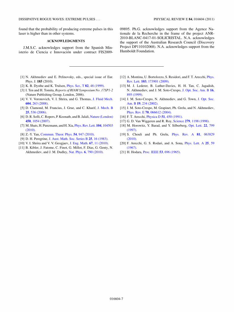
An important issue in defining rogue waves is the levelof the significant wave height (SWH). The latter requires theknowledge of the probability of appearance of waves of allamplitudes, starting from the zero level. This is problematicas the PDF in our case does not have a constant limit atlow intensities. Instead, it increases to high value that maydepend on many factors, including the size of the numericalgrid. Thus, counting the total number of events requiredfor the calculation of the SWH is complicated. In order toovercome this difficulty, we have to remove small-intensitypulses below a certain threshold from consideration. Thisthreshold, say Imin, is one of the essential parameters inthe definition of the SWH and consequently of the roguewave.

In order to show that, we calculated the SWH for variouslevels of the threshold intensity, Imin. The results are shown inFig. 12. Here, the blue dotted line represents the SWH versusImin. Despite the fact that the SWH decreases indefinitely whenwe decrease the Imin, the straight-line approximation from thehigh-intensity part of the curve provides us with the roughestimate of the SWH being around 4. This approximate valuecan be used for the definition of the minimum intensity of arogue wave, which is normally (using the common definitiontaken for ocean waves) 2.2 times the SWH, that is, 8.8 in ourcase.

The red dashed line in Fig. 12 shows the probability of theappearance of a pulse with an intensity above this level. As wecan see from the figure, this probability is relatively high. Evenif we choose an unreasonably high value of Imin, ignoring mostof the low-amplitude pulses, this probability is above 0.001.The lower limit of the probability is above 0.01. Thus, extremepulses in dissipative systems may appear quite often. Roughlyspeaking, every pulse out of a hundred can be counted as beingextreme. This probability is significantly higher than in any ofthe systems considered so far.

In conclusion, we considered a typical fiber laser cavity ina regime of generating multipulse sequences. At certain sets ofparameters, the laser can serve as an example of a dissipativesystem which transforms a continuous pump of energy intoa chaotic train of pulses with random amplitudes. We have

016604-6

DISSIPATIVE ROGUE WAVES: EXTREME PULSES . . . PHYSICAL REVIEW E 84, 016604 (2011)

found that the probability of producing extreme pulses in thislaser is higher than in other systems.

ACKNOWLEDGMENTS

J.M.S.C. acknowledges support from the Spanish Min-isterio de Ciencia e Innovacion under contract FIS2009-

09895. Ph.G. acknowledges support from the Agence Na-tionale de la Recherche in the frame of the project ANR-2010-BLANC-0417-01-SOLICRISTAL. N.A. acknowledgesthe support of the Australian Research Council (DiscoveryProject DP110102068). N.A. acknowledges support from theHumboldt Foundation.

[1] N. Akhmediev and E. Pelinovsky, eds., special issue of Eur.Phys. J. 185 (2010).

[2] K. B. Dysthe and K. Trulsen, Phys. Scr., T 82, 48 (1999).[3] I. Ten and H. Tomita, Reports of RIAM Symposium No. 17SP1-2

(Nature Publishing Group, London, 2006).[4] V. V. Voronovich, V. I. Shrira, and G. Thomas, J. Fluid Mech.

604, 263 (2008).[5] D. Clamond, M. Francius, J. Grue, and C. Kharif, J. Mech. B

25, 536 (2006).[6] D. R. Solli, C. Ropers, P. Koonath, and B. Jalali, Nature (London)

450, 1054 (2007).[7] M. Shats, H. Punzmann, and H. Xia, Phys. Rev. Lett. 104, 104503

(2010).[8] Z.-Y. Yan, Commun. Theor. Phys. 54, 947 (2010).[9] D. H. Peregrine, J. Aust. Math. Soc. Series B 25, 16 (1983).

[10] V. I. Shrira and V. V. Geogjaev, J. Eng. Math. 67, 11 (2010).[11] B. Kibler, J. Fatome, C. Finot, G. Millot, F. Dias, G. Genty, N.

Akhmediev, and J. M. Dudley, Nat. Phys. 6, 790 (2010).

[12] A. Montina, U. Bortolozzo, S. Residori, and F. T. Arecchi, Phys.Rev. Lett. 103, 173901 (2009).

[13] M. J. Lederer, B. Luther-Davies, H. H. Tan, C. Jagadish,N. Akhmediev, and J. M. Soto-Crespo, J. Opt. Soc. Am. B 16,895 (1999).

[14] J. M. Soto-Crespo, N. Akhmediev, and G. Town, J. Opt. Soc.Am. B 19, 234 (2002).

[15] J. M. Soto-Crespo, M. Grapinet, Ph. Grelu, and N. Akhmediev,Phys. Rev. E 70, 066612 (2004).

[16] F. T. Arecchi, Physica D 51, 450 (1991).[17] G. D. Van Wiggeren and R. Roy, Science 279, 1198 (1998).[18] M. Horowitz, Y. Barad, and Y. Silberberg, Opt. Lett. 22, 799

(1997).[19] S. Chouli and Ph. Grelu, Phys. Rev. A 81, 063829

(2010).[20] F. Arecchi, G. S. Rodari, and A. Sona, Phys. Lett. A 25, 59

(1967).[21] H. Hodara, Proc. IEEE 53, 696 (1965).

016604-7