Properties of Walrasian Demand

Econ 2100 Fall 2017

Lecture 5, September 12

Problem Set 2 is due in Kelly’s mailbox by 5pm today

Outline

1 Properties of Walrasian Demand2 Indirect Utility Function3 Envelope Theorem

Summary of Constrained Optimization

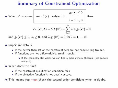
When x∗ is solvesgi (x) ≤ 0

max f (x) subject toi = 1, ..,m

then

∇L (x∗,λ) = ∇f (x∗)−m∑i=1

λi∇gi (x∗) = 0

and gi (x∗) ≤ 0, λi ≥ 0, and λigi (x∗) = 0 for i = 1, ...,m.

Important details:

If the better than set or the constraint sets are not convex: big trouble.If functions are not differentiable: small trouble.

If the geometry still works we can find a more general theorem (see convexanalysis).

When does this fail?

If the constraint qualification condition fails.If the objective function is not quasi concave.

This means you must check the second order conditions when in doubt.

Walrasian Demand

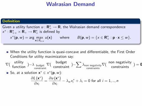
DefinitionGiven a utility function u : Rn+ → R, the Walrasian demand correspondencex∗ : Rn++ × R+ → Rn+ is defined by

x∗(p,w) = arg maxx∈Bp,w

u(x) where B(p,w) = {x ∈ Rn+ : p · x ≤ w}.

When the utility function is quasi-concave and differentiable, the First OrderConditions for utility maximization say:

∇(utilityfunction

)−λ budgetconstraint

∇(budgetconstraint

)−∑

λnon negativityconstraints

∇(non negativityconstraints

) = 0

So, at a solution x∗ ∈ x∗(p,w):∂L (x∗)∂xi

=∂u (x∗)∂xi

− λw x∗i + λi = 0 for all i = 1, .., n

Marginal Rate of Substitution

Suppose we have an optimal consumption bundle x∗ where some goods areconsumed in strictly positive amounts.

Then, the corresponding non-negativity constraints hold and the correspodingmultipliers equal 0.

At such a solution x∗, the first order condition is:∂u (x∗)∂xi

= λw pi for all i such that x∗i > 0

This expression implies∂u(x∗)∂xj

∂u(x∗)∂xk

=pjpk

for any j , k such that x∗j , x∗k > 0

This is the familiar condition about equalizing marginal rates of substituitonsto price ratios.

Marginal Utility Per Dollar SpentAt an optimal consumption bundle x∗ where some goods are consumed instrictly positive amounts, the first order condition is:

∂u (x∗)∂xi

= λw pi for all i such that x∗i > 0

Another way to rearrange it gives∂u(x∗)∂xj

pj=

∂u(x∗)∂xk

pkfor any j , k such that x∗j , x

∗k > 0

the marginal utility per dollar spent must be equal across goods.

If not, there are j and k for which∂u(x∗)∂xjpj

<∂u(x∗)∂xkpk

DM can buy εpjless of j , and ε

pkmore of k , so the budget constraint still holds,

andby Taylor’s theorem, the utility at the new choice is

u (x∗)+∂u (x∗)∂xj

(− ε

pj

)+∂u (x∗)∂xk

(ε

pk

)+o (ε) = u (x∗)+ε

∂u(x∗)∂xk

pk−

∂u(x∗)∂xj

pj

+o (ε)which implies that x∗ is not an optimum.

Think about the case in which some goods are consumed in zero amount.

Demand and Indirect Utility FunctionThe Walrasian demand correspondence x∗ : Rn++ × R+ → Rn+ is defined by

x∗(p,w) = arg maxx∈B(p,w )

u(x) where B(p,w) = {x ∈ Rn+ : p · x ≤ w}.

DefinitionGiven a continuous utility function u : Rn+ → R, the indirect utility functionv : Rn++ × R+ → R is defined by

v(p,w) = u(x∗) where x∗ ∈ x∗(p,w).

The indirect utility function measures changes in the ‘optimized’value of theobjective function as the parameters (prices and wages) change and theconsumer adjusts her optimal consumption accordingly.

ResultsThe Walrasian demand correspondence is upper hemi continuous

To prove this we need properties that characterize continuity forcorrespondences.

The indirect utility function is continuous.

To prove this we need properties that characterize continuity forcorrespondences.

Berge’s Theorem of the MaximumThe theorem of the maximum lets us establish the previous two results.

Theorem (Theorem of the Maximum)

If f : X → R is a continuous function and ϕ : Q → X is a continuouscorrespondence with nonempty and compact values, then

the mapping x∗ : Q → X defined by

x∗(q) = arg maxx∈ϕ(q)

f (x)

is an upper hemicontinuous correspondence and

the mapping v : Q → R defined byv(q) = max

x∈ϕ(q)f (x)

is a continuous function.

Berge’s Theorem is useful when exogenous parameters enter the optimizationproblem only through the constraints, and do not directly enter the objectivefunction.This happens in the consumer’s problem: prices and income do not enter theutility function, they only affect the budget set.

Properties of Walrasian Demand

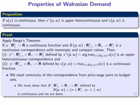
Proposition

If u(x) is continuous, then x∗(p,w) is upper hemicontinuous and v(p,w) iscontinuous.

Proof.Apply Berge’s Theorem:If u : Rn+ → R a continuous function and B (p,w) : Rn++ × R+ → Rn+ is acontinuous correspondence with nonempty and compact values. Then:(i): x∗ : Rn++ × R+ → Rn+ defined by x∗(p,w) = argmaxx∈B(p,w ) u(x) is an upperhemicontinuous correspondence and(ii): v : Rn++ × R+ → R defined by v(p,w) = maxx∈B(p,w ) u(x) is a continuousfunction.

We need continuity of the correspondence from price-wage pairs to budgetsets.

We must show that B : Rn++ × R+ → Rn+ defined byB(p,w ) = {x ∈ Rn+ : p · x ≤ w}

is continuous and we are done.

Continuity for Correspondences

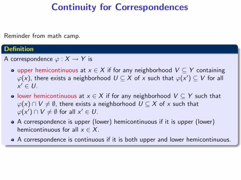
Reminder from math camp.

DefinitionA correspondence ϕ : X → Y is

upper hemicontinuous at x ∈ X if for any neighborhood V ⊆ Y containingϕ(x), there exists a neighborhood U ⊆ X of x such that ϕ(x ′) ⊆ V for allx ′ ∈ U.lower hemicontinuous at x ∈ X if for any neighborhood V ⊆ Y such thatϕ(x) ∩ V 6= ∅, there exists a neighborhood U ⊆ X of x such thatϕ(x ′) ∩ V 6= ∅ for all x ′ ∈ U.A correspondence is upper (lower) hemicontinuous if it is upper (lower)hemicontinuous for all x ∈ X .A correspondence is continuous if it is both upper and lower hemicontinuous.

Conditions for Continuity (from Math Camp)

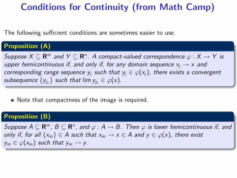
The following suffi cient conditions are sometimes easier to use.

Proposition (A)

Suppose X ⊆ Rm and Y ⊆ Rn . A compact-valued correspondence ϕ : X → Y isupper hemicontinuous if, and only if, for any domain sequence xj → x andcorresponding range sequence yj such that yj ∈ ϕ(xj ), there exists a convergentsubsequence {yjk } such that lim yjk ∈ ϕ(x).

Note that compactness of the image is required.

Proposition (B)

Suppose A ⊆ Rm , B ⊆ Rn , and ϕ : A→ B. Then ϕ is lower hemicontinuous if, andonly if, for all {xm} ∈ A such that xm → x ∈ A and y ∈ ϕ(x), there existym ∈ ϕ(xm) such that ym → y.

Continuity for Correspondences: Examples

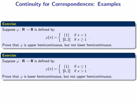
ExerciseSuppose ϕ : R→ R is defined by:

ϕ(x) =

{{1} if x < 1

[0, 2] if x ≥ 1 .

Prove that ϕ is upper hemicontinuous, but not lower hemicontinuous.

ExerciseSuppose ϕ : R→ R is defined by:

ϕ(x) =

{{1} if x ≤ 1

[0, 2] if x > 1.

Prove that ϕ is lower hemicontinuous, but not upper hemicontinuous.

Continuity of the Budget Set Correspondence

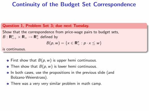
Question 1, Problem Set 3; due next Tuesday.Show that the correspondence from price-wage pairs to budget sets,B : Rn++ × R+ → Rn+ defined by

B(p,w) = {x ∈ Rn+ : p · x ≤ w}is continuous.

First show that B(p,w) is upper hemi continuous.

Then show that B(p,w) is lower hemi continuous.

In both cases, use the propositions in the previous slide (andBolzano-Weierstrass).

There was a very very similar problem in math camp.

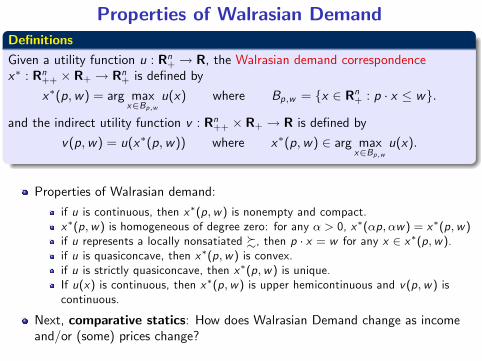
Properties of Walrasian DemandDefinitionsGiven a utility function u : Rn+ → R, the Walrasian demand correspondencex∗ : Rn++ × R+ → Rn+ is defined by

x∗(p,w) = arg maxx∈Bp,w

u(x) where Bp,w = {x ∈ Rn+ : p · x ≤ w}.

and the indirect utility function v : Rn++ × R+ → R is defined byv(p,w) = u(x∗(p,w)) where x∗(p,w) ∈ arg max

x∈Bp,wu(x).

Properties of Walrasian demand:

if u is continuous, then x∗(p,w ) is nonempty and compact.x∗(p,w ) is homogeneous of degree zero: for any α > 0, x∗(αp, αw ) = x∗(p,w )if u represents a locally nonsatiated %, then p · x = w for any x ∈ x∗(p,w ).if u is quasiconcave, then x∗(p,w ) is convex.if u is strictly quasiconcave, then x∗(p,w ) is unique.If u(x) is continuous, then x∗(p,w ) is upper hemicontinuous and v (p,w ) iscontinuous.

Next, comparative statics: How does Walrasian Demand change as incomeand/or (some) prices change?

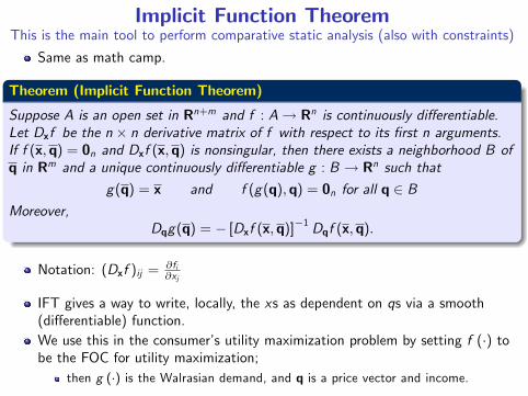
Implicit Function TheoremThis is the main tool to perform comparative static analysis (also with constraints)

Same as math camp.

Theorem (Implicit Function Theorem)

Suppose A is an open set in Rn+m and f : A→ Rn is continuously differentiable.Let Dxf be the n × n derivative matrix of f with respect to its first n arguments.If f (x,q) = 0n and Dxf (x,q) is nonsingular, then there exists a neighborhood B ofq in Rm and a unique continuously differentiable g : B → Rn such that

g(q) = x and f (g(q),q) = 0n for all q ∈ BMoreover,

Dqg(q) = − [Dxf (x,q)]−1 Dqf (x,q).

Notation: (Dxf )ij = ∂fi∂xj

IFT gives a way to write, locally, the xs as dependent on qs via a smooth(differentiable) function.We use this in the consumer’s utility maximization problem by setting f (·) tobe the FOC for utility maximization;

then g (·) is the Walrasian demand, and q is a price vector and income.

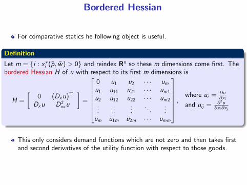
Bordered Hessian

For comparative statics he following object is useful.

Definition

Let m = {i : x∗i (p̄, w̄) > 0} and reindex Rn so these m dimensions come first. Thebordered Hessian H of u with respect to its first m dimensions is

H =

[0 (Dxu)>

Dxu D2xxu

]=

0 u1 u2 · · · umu1 u11 u21 · · · um1u2 u12 u22 · · · um2...

......

. . ....

um u1m u2m · · · umm

,where ui = ∂u

∂xi

and uij = ∂2u∂xi∂xj

This only considers demand functions which are not zero and then takes firstand second derivatives of the utility function with respect to those goods.

Differentiability of Walrasian Demand

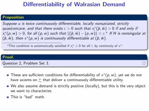
PropositionSuppose u is twice continuously differentiable, locally nonsatiated, strictlyquasiconcave, and that there exists ε > 0 such that x∗i (p̄, w̄) > 0 if and only ifx∗i (p,w) > 0, for all (p,w) such that ‖(p̄, w̄)− (p,w)‖ < ε.a If H is nonsingular at(p̄, w̄), then x∗(p,w) is continuously differentiable at (p̄, w̄).

aThis condition is automatically satisfied if x∗i > 0 for all i , by continuity of x∗.

Proof.Question 2, Problem Set 3.

These are suffi cient conditions for differentiability of x∗(p,w), yet we do nothave axioms on % that deliver a continuously differentiable utility.We also assume demand is strictly positive (locally), but this is the very objectwe want to characterize.

This is “bad”math.

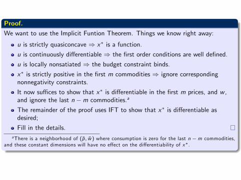
Proof.We want to use the Implicit Funtion Theorem. Things we know right away:

u is strictly quasiconcave ⇒ x∗ is a function.

u is continuously differentiable ⇒ the first order conditions are well defined.

u is locally nonsatiated ⇒ the budget constraint binds.

x∗ is strictly positive in the first m commodities ⇒ ignore correspondingnonnegativity constraints.

It now suffi ces to show that x∗ is differentiable in the first m prices, and w ,and ignore the last n −m commodities.a

The remainder of the proof uses IFT to show that x∗ is differentiable asdesired;

Fill in the details.aThere is a neighborhood of (p̄, w̄ ) where consumption is zero for the last n −m commodities,

and these constant dimensions will have no effect on the differentiability of x∗.

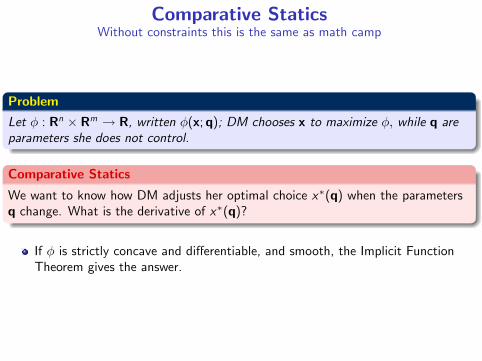
Comparative StaticsWithout constraints this is the same as math camp

Problem

Let φ : Rn × Rm → R, written φ(x;q); DM chooses x to maximize φ, while q areparameters she does not control.

Comparative Statics

We want to know how DM adjusts her optimal choice x∗(q) when the parametersq change. What is the derivative of x∗(q)?

If φ is strictly concave and differentiable, and smooth, the Implicit FunctionTheorem gives the answer.

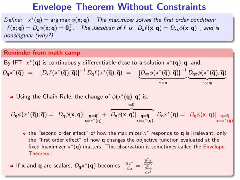
Envelope Theorem Without ConstraintsDefine: x∗(q) = argmaxφ(x;q). The maximizer solves the first order condition:f (x;q) = Dxφ(x;q) = 0>n . The Jacobian of f is Dxf (x;q) = Dxxφ(x;q) , and isnonsingular (why?).

Reminder from math camp

By IFT: x∗(q) is continuously differentiable close to a solution x∗(q),q, and:

Dqx∗(q) = − [Dxf (x∗(q);q)]−1 Dqf (x∗(q);q) = − [Dxxφ(x∗(q);q)]−1︸ ︷︷ ︸n×n

Dqxφ(x∗(q);q)︸ ︷︷ ︸n×m

Using the Chain Rule, the change of φ(x∗(q);q) is:

Dqφ(x∗(q);q) = Dqφ(x,q)| q=qx=x∗(q)

+

=0︷ ︸︸ ︷Dxφ(x,q)| q=q

x=x∗(q)

Dqx∗(q) = Dqφ(x,q)| q=qx=x∗(q)

the “second order effect” of how the maximizer x∗ responds to q is irrelevant; onlythe “first order effect” of how q changes the objective function evaluated at thefixed maximizer x∗(q) matters. This observation is sometimes called the EnvelopeTheorem.

If x and q are scalars, Dqx∗(q) becomes ∂x∗

∂q =∂2φ∂q∂x∂2φ∂x2

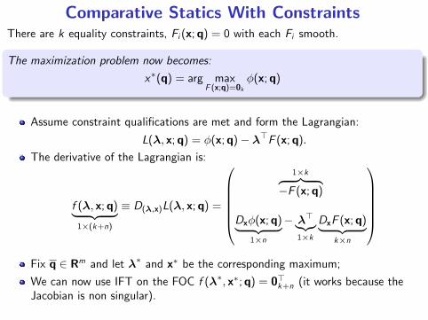
Comparative Statics With ConstraintsThere are k equality constraints, Fi (x;q) = 0 with each Fi smooth.

The maximization problem now becomes:

x∗(q) = arg maxF (x;q)=0k

φ(x;q)

Assume constraint qualifications are met and form the Lagrangian:

L(λ, x;q) = φ(x;q)− λ>F (x;q).

The derivative of the Lagrangian is:

f (λ, x;q)︸ ︷︷ ︸1×(k+n)

≡ D(λ,x)L(λ, x;q) =

1×k︷ ︸︸ ︷

−F (x;q)

Dxφ(x;q)︸ ︷︷ ︸1×n

− λ>︸︷︷︸1×k

DxF (x;q)︸ ︷︷ ︸k×n

Fix q ∈ Rm and let λ∗ and x∗ be the corresponding maximum;We can now use IFT on the FOC f (λ∗, x∗;q) = 0>k+n (it works because theJacobian is non singular).

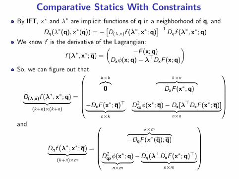
Comparative Statics With ConstraintsBy IFT, x∗ and λ∗ are implicit functions of q in a neighborhood of q, and

Dq(λ∗(q), x∗(q)) = −[D(λ,x)f (λ∗, x∗;q)

]−1Dq f (λ∗, x∗;q)

We know f is the derivative of the Lagrangian:

f (λ∗, x∗;q) =

(−F (x;q)

Dxφ(x;q)− λ>DxF (x;q)

)So, we can figure out that

D(λ,x)f (λ∗, x∗;q)︸ ︷︷ ︸(k+n)×(k+n)

=

k×k︷︸︸︷0

k×n︷ ︸︸ ︷−DxF (x∗;q)

−DxF (x∗;q)>︸ ︷︷ ︸n×k

D2xxφ(x∗;q)− Dx[λ>DxF (x∗;q)]︸ ︷︷ ︸n×n

and

Dq f (λ∗, x∗;q)︸ ︷︷ ︸(k+n)×m

=

k×m︷ ︸︸ ︷

−DqF (x∗(q);q)

D2qxφ(x∗;q)︸ ︷︷ ︸n×m

−Dq(λ>DxF (x∗;q)>)︸ ︷︷ ︸n×m

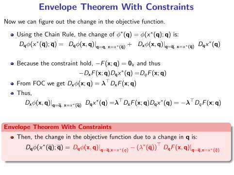
Envelope Theorem With ConstraintsNow we can figure out the change in the objective function.

Using the Chain Rule, the change of φ∗(q) = φ(x∗(q);q) is:

Dqφ(x∗(q);q) = Dqφ(x,q)|q=q, x=x∗(q) + Dxφ(x,q)|q=q, x=x∗(q) Dqx∗(q)

Because the constraint hold, −F (x;q) = 0k and thus−DxF (x;q)Dqx∗(q) =DqF (x;q)

From FOC we get Dxφ(x;q) = λ>DxF (x;q)

Thus,

Dxφ(x,q)|q=q, x=x∗(q) Dqx∗(q) =λ>DxF (x;q)Dqx∗(q) = −λ>DqF (x;q)

Envelope Theorem With ConstraintsThen, the change in the objective function due to a change in q is:

Dqφ(x∗(q);q) = Dqφ(x,q)|q=q,x=x∗(q) − (λ∗(q))> DqF (x,q)|q=q,x=x∗(q̄)