Properties of Random Direction Models

Philippe Nain, Don Towsley, Benyuan Liu, Zhen Liu

Main mobility models

Random Waypoint

Random Direction

Random Waypoint

Pick location x at random Go to x at constant speed v

Stationary distribution of node

location not uniform in area

Random Direction

Pick direction θ at random

Move in direction θ at constant speed v for time τ

Upon hitting boundary reflection or wrap around

Reflection in 2D

Wrap around in 2D

Question:

Under what condition(s) stationary distribution of node location uniform over area?

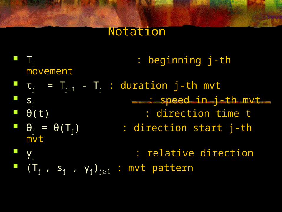
Notation

Tj : beginning j-th movement τj = Tj+1 - Tj : duration j-th mvt sj : speed in j-th mvt θ(t) : direction time t θj = θ(Tj) : direction start j-th mvt γj : relative direction (Tj , sj , γj)j1 : mvt pattern

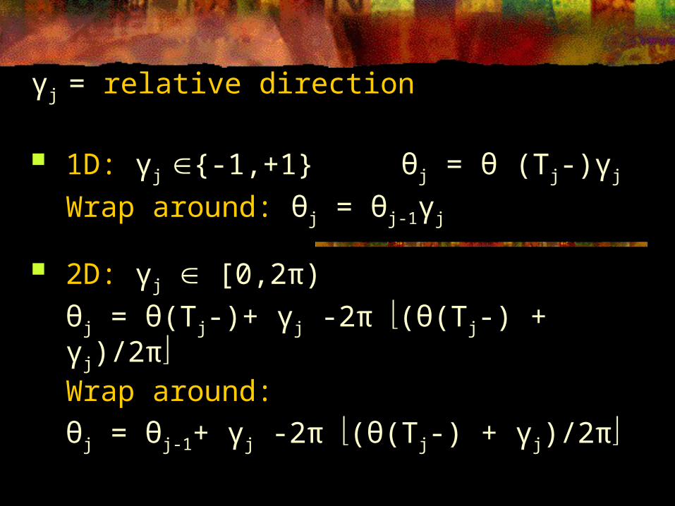
γj = relative direction

1D: γj {-1,+1} θj = θ (Tj-)γj

Wrap around: θj = θj-1γj

2D: γj [0,2π)

θj = θ(Tj-)+ γj -2π (θ(Tj-) + γj)/2πWrap around:

θj = θj-1+ γj -2π (θ(Tj-) + γj)/2π

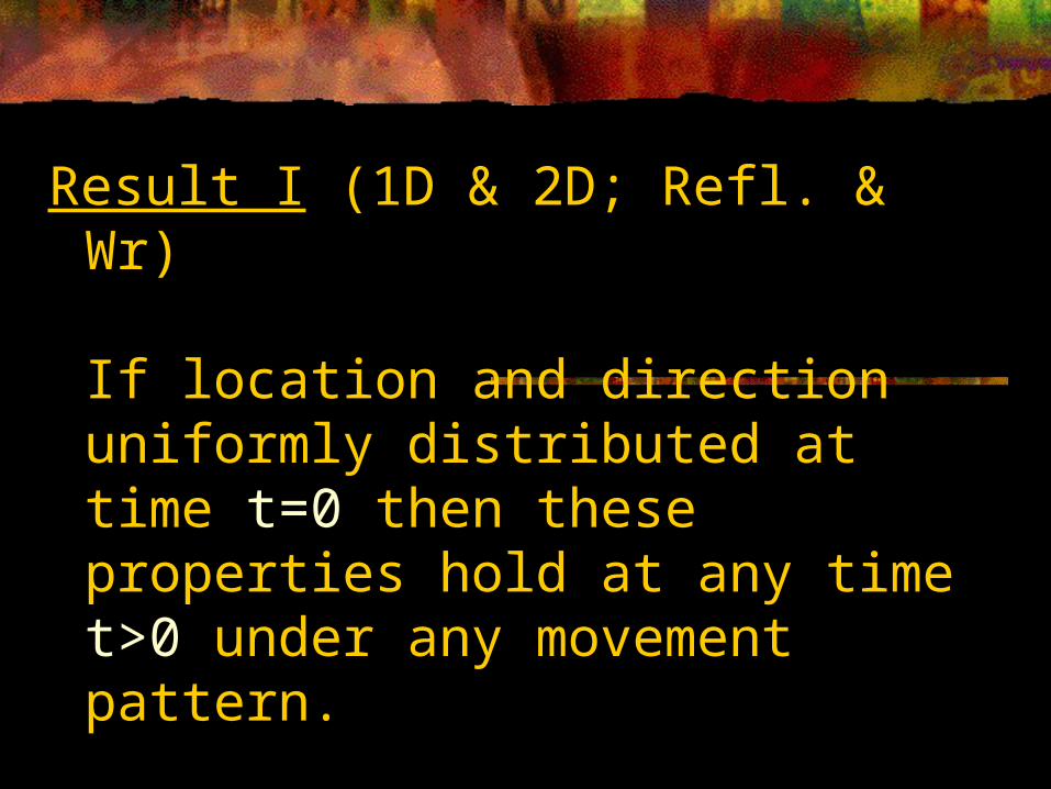
Result I (1D & 2D; Refl. & Wr)

If location and direction uniformly distributed at time t=0 then these properties hold at any time t>0 under any movement pattern.

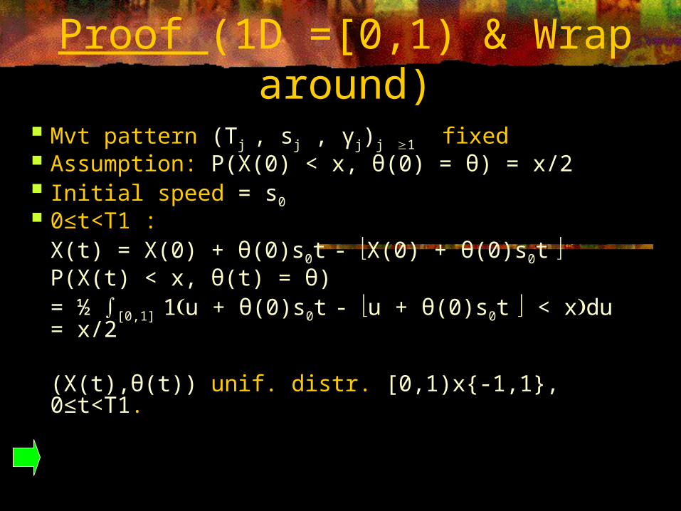
Proof (1D =[0,1) & Wrap around) Mvt pattern (Tj , sj , γj)j 1 fixed Assumption: P(X(0) < x, θ(0) = θ) = x/2 Initial speed = s0 0≤t<T1 :

X(t) = X(0) + θ(0)s0t - X(0) + θ(0)s0t P(X(t) < x, θ(t) = θ) = ½ ∫[0,1] 1u + θ(0)s0t - u + θ(0)s0t < xdu = x/2

(X(t),θ(t)) unif. distr. [0,1)x{-1,1}, 0≤t<T1.

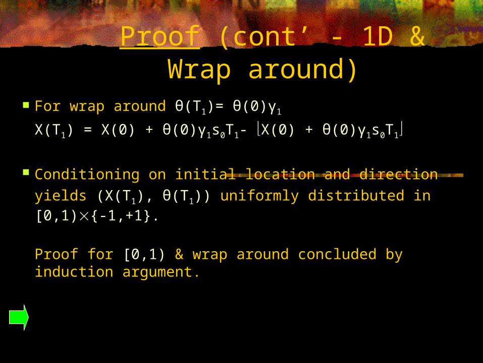
Proof (cont’ - 1D & Wrap around) For wrap around θ(T1)= θ(0)γ1

X(T1) = X(0) + θ(0)γ1s0T1- X(0) + θ(0)γ1s0T1

Conditioning on initial location and direction

yields (X(T1), θ(T1)) uniformly distributed in [0,1){-1,+1}.

Proof for [0,1) & wrap around concluded by induction argument.

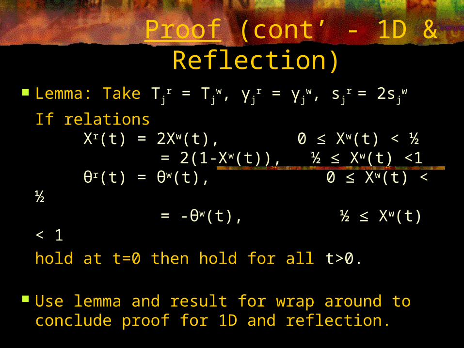
Proof (cont’ - 1D & Reflection) Lemma: Take Tj

r = Tjw, γj

r = γjw, sj

r = 2sjw

If relations Xr(t) = 2Xw(t), 0 ≤ Xw(t) < ½ = 2(1-Xw(t)), ½ ≤ Xw(t) <1 θr(t) = θw(t), 0 ≤ Xw(t) < ½ = -θw(t), ½ ≤ Xw(t) < 1

hold at t=0 then hold for all t>0.

Use lemma and result for wrap around to conclude proof for 1D and reflection.

Proof (cont’ - 2D Wrap around & reflection)

. Area: rectangle, disk, …

Wrap around: direct argument like in 1D

Reflection: use relation between wrap around & reflection – See Infocom’05 paper.

Corollary

N mobiles unif. distr. on [0,1] (or [0,1]2) with equally likely orientation at t=0

Mobiles move independently of each other

Mobiles uniformly distributed with equally likely orientation for all t>0.

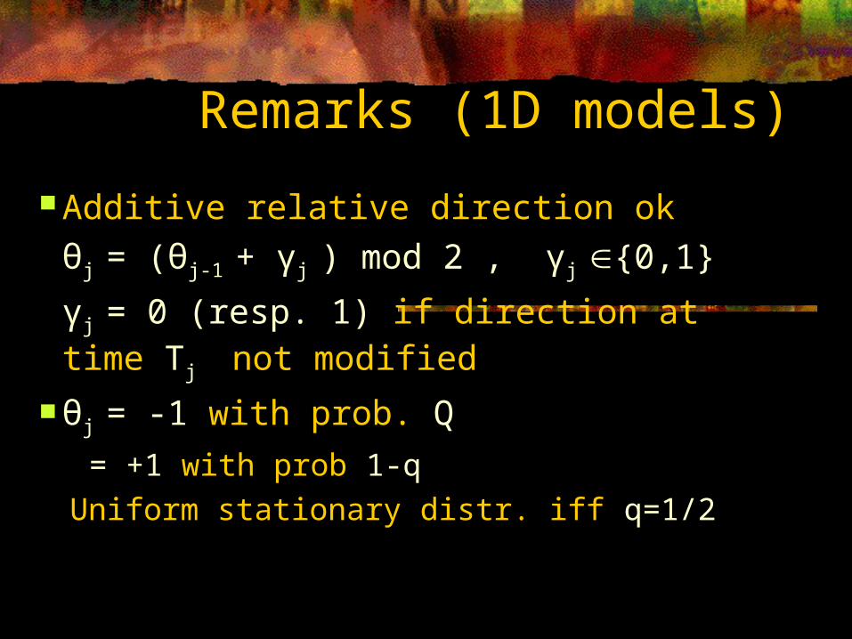
Remarks (1D models)

Additive relative direction ok

θj = (θj-1 + γj ) mod 2 , γj {0,1}

γj = 0 (resp. 1) if direction at time Tj not modified

θj = -1 with prob. Q

= +1 with prob 1-q

Uniform stationary distr. iff q=1/2

How can mobiles reach uniformstationary distributions for location and orientation starting from any initial state?

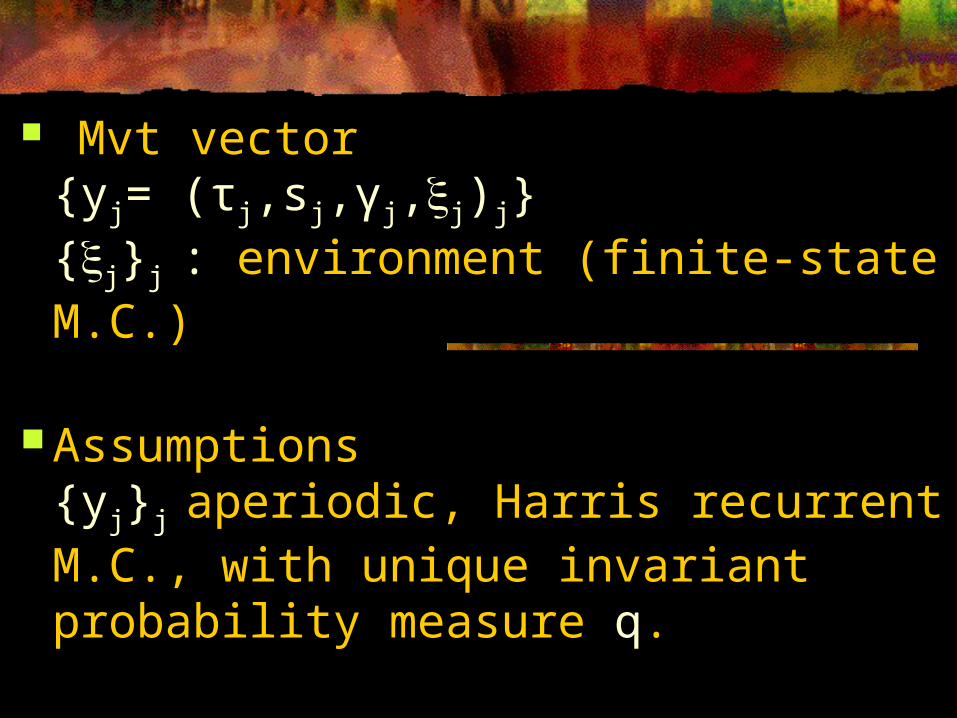
Mvt vector {yj= (τj,sj,γj,j)j}{j}j : environment (finite-state M.C.)

Assumptions{yj}j aperiodic, Harris recurrent M.C., with unique invariant probability measure q.

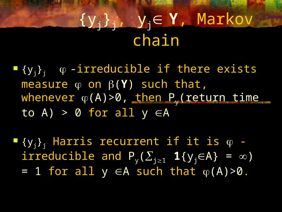
{yj}j, yj Y, Markov chain

{yj}j -irreducible if there exists measure on (Y) such that, whenever (A)>0, then Py(return time to A) > 0 for all y A

{yj}j Harris recurrent if it is -irreducible and Py(j1 1{yjA} = ) = 1 for all y A such that (A)>0.

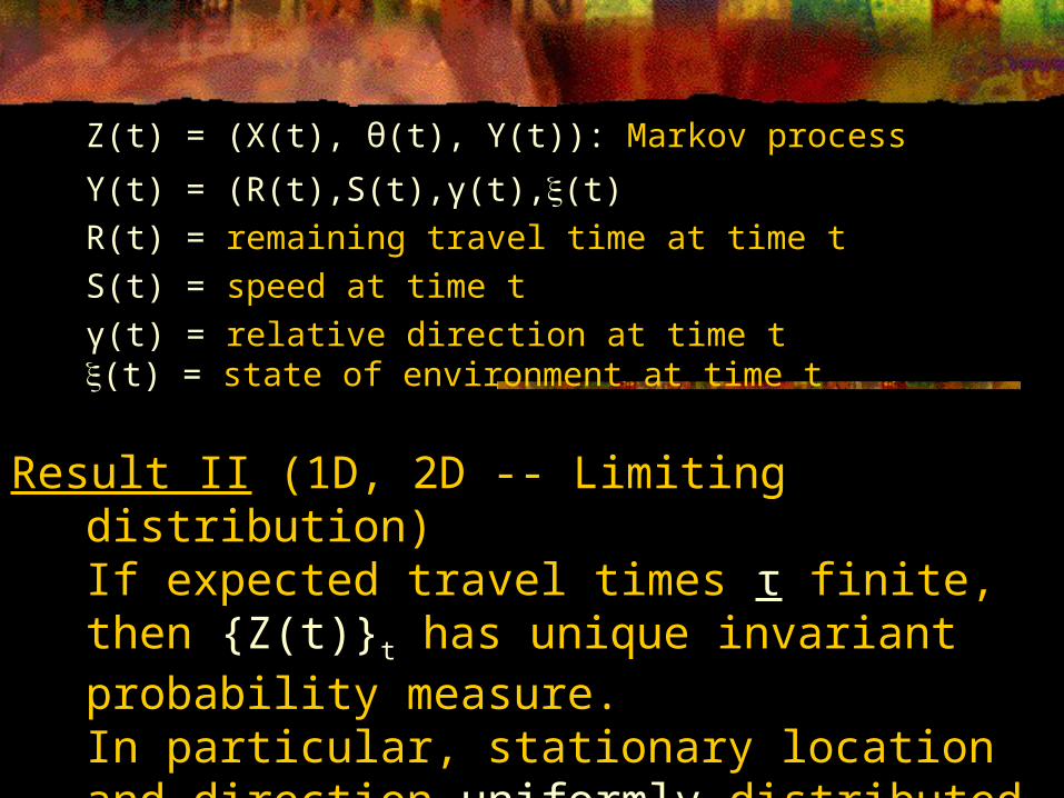
Z(t) = (X(t), θ(t), Y(t)): Markov process

Y(t) = (R(t),S(t),γ(t),(t)

R(t) = remaining travel time at time t

S(t) = speed at time t

γ(t) = relative direction at time t(t) = state of environment at time t

Result II (1D, 2D -- Limiting distribution)If expected travel times τ finite, then {Z(t)}t has unique invariant probability measure. In particular, stationary location and direction uniformly distributed.

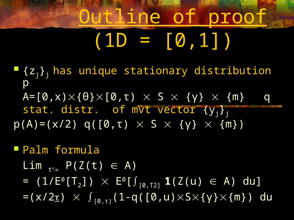
Outline of proof (1D = [0,1]) {zj}j has unique stationary distribution p

A=[0,x){θ}[0,τ) S {γ} {m} q stat. distr. of mvt vector {yj}j

p(A)=(x/2) q([0,τ) S {γ} {m})

Palm formula

Lim t P(Z(t) A)

= (1/E0[T2]) E0[∫[0,T2] 1(Z(u) A) du]

=(x/2) ∫[0,τ)(1-q([0,u)S{γ}{m}) du

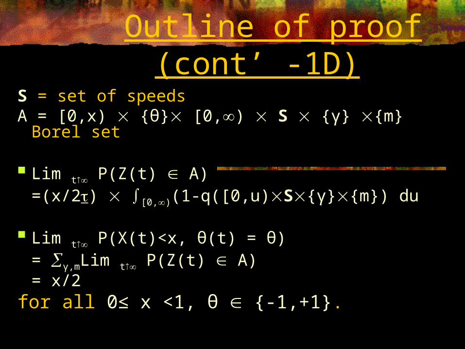
Outline of proof (cont’ -1D)S = set of speeds A = [0,x) {θ} [0,) S {γ} {m} Borel set

Lim t P(Z(t) A)=(x/2) ∫[0,)(1-q([0,u)S{γ}{m}) du

Lim t P(X(t)<x, θ(t) = θ) = γ,mLim t P(Z(t) A)= x/2

for all 0≤ x <1, θ {-1,+1}.

Outline of proof (cont’ -2D = [0,1]2) Same proof as for 1D except that set

of directions is now [0,2)

Lim t P(X1(t)<x1, X2(t)<x2, θ(t)< θ)

= x1x2 θ/2

for all 0≤ x1, x2 <1, θ [0,2).

Assumptions hold if (for instance): Speeds and relative directions mutually

independent renewal sequences, independent of travel times and environment {τj ,j}j

Travel times modulated by {j}j , jM:{τj (m)}j , mM, independent renewal sequences, independent of {sj , γj ,j}j, with density and finite expectation.

ns-2 module available from authors

Sorry, it’s finished