Production of the S¯0 hyperons in the PANDA experiment at...
111
Production of the ¯ Σ 0 hyperons in the PANDA experiment at FAIR Master Programme in Physics Degree thesis Uppsala University Department of Physics and Astronomy Author: Gabriela Pérez Andrade Supervisor: Karin Schönning
Transcript of Production of the S¯0 hyperons in the PANDA experiment at...
Production of the Σ0 hyperons in the PANDA experiment at FAIR
Master Programme in PhysicsDegree thesis
Uppsala UniversityDepartment of Physics and Astronomy
Author: Gabriela Pérez AndradeSupervisor: Karin Schönning
I
Abstract
The PANDA experiment is one of the main pillars of the Facility for Antiproton and IonResearch (FAIR), currently under construction in Darmstadt, Germany. PANDA will bea fixed target experiment designed for the study of non-perturbative phenomena of thestrong interaction. Strange hyperon production is governed by ms ∼ 100 MeV, whichcorresponds to the confinement domain. Thus, hyperons are suitable probes in thisenergy region. This work is a simulation study focused on the feasibility of studying theproduction of Σ0 and Λ hyperons in the pp→ Σ0Λ reaction with the PANDA detector.A 104 events sample simulated at pbeam = 1.771 GeV/c is used to perform a single-tag(inclusive) and a double-tag (exclusive) event selection. From the former, it is concludedthat the single-tag method does not provide with the clean signal required for spinobservables extraction. In contrast, exclusive event selection provides with a signalreasonably clean from combinatorial background and completely clean from generichadronic background events. A signal (Σ0Λ) reconstruction efficiency of ε = 5.3 ± 0.2 %is obtained for exclusive event selection. The corresponding signal to background ratiois S/BTotal ∼6 and the significance value is ∼21.In addition, an exclusive event selection is performed on a 104 events sample simulatedat pbeam = 6 GeV/c. Almost all the generic hadronic background events are removed bythe applied selection criteria. At this beam momentum, the obtained signal efficiency isε = 6.1 ± 0.3%, the signal to total background ratio is S/BTotal ∼ 4 and the significanceis ∼22. Both efficiencies are smaller compared to a previous simulation study on thischannel, but are large enough to enable a study of the exclusive production of thepp→ Σ0Λ reaction at PANDA. The difference between the results of this thesis workand the previous work is attributed to the more realistic implementation of the signalproduction mechanism, as well as the detector and reconstruction algorithms.
II
Acknowledgements
After being in Sweden for more than two years, there are many people I would like tothank. I was tempted to keep it short and simply express a very special thank you to all myfamily and friends. But I am Mexican, I can’t. So here I go.First of all, I would like to thank my supervisor Karin Schönning for giving me theopportunity of being part of her group and encouraging me to give my best. Thanks forall the invested time and the opportunities of attending the PANDA-meetings. I deeplyappreciate all the support. Thanks to Stefan Leupold for taking the time to read thiswork and comment on it. To Michael Papenbrock and Tord Johansson for the guidanceand comments during rehearsal talks or questions in general. I learned a lot from all ofyou and you represent a great inspiration for me.Thanks to my family. Every and each member of it. Special thanks to my father Enriqueand my mother Mirna who since the beginning of times have encouraged me to pursuemy dreams and taught me that it is (almost) all about effort. To my sister Daniela, mybrother Jonathan and cousin Itaviany, for always being there for me when I needed. ToDaniel Alberto, who has been with me in every step of this way, from applying to UUuntil the last day I worked in this thesis. Thank you for listening to me and being one ofthe biggest supports and motivations I have.Thanks to Marianne, Sam, Sammy and Ale for all these years of friendship, in which nomatter if I am 139 km, 628 km or 9,522 km away, they always find the way of makingme part of their life. To my UNAM-family: Laura, Dario, Mady, Arturo, AJ and RafaelAlberto, thanks for listening to me and giving me advice about all mental tangles thatcould cross my mind (personal or physics-related). Thanks to Lalo, Soco, Fernando,Tiff, Esteban and Citlali because those sporadic chats were always very special. To myLEMA-family: Corina Solís, Luis Acosta and Efraín Chávez for their trust and big moraland academic backing whenever I needed. To all of you, thanks for arriving and staying.Sweden has given me the opportunity of meeting extraordinary people at differentstages, and whose presence has been crucial at certain points of this path. I start withthanking Jonatan Fast, who made me feel welcome and inevitably I tagged as my friendsince day-one in Sweden. Thanks to Yajie for being the best company to carry out thefirst simple tasks that represented a great change for me (like riding a bike for the firsttime in several years).Marika and Konstantinos, thanks for the long talks, the movies and the shared time inthe basement. I cannot imagine my days here without you. To my friends who helpedme and in different ways always cared about my wellbeing, Paulius, Benjamin, Linda,Daniel, Matthias, Christine and Vasilis, thank you.
III
To my Latin-American family: Silvia, Sol, David, Thaís and Esteban: ¡Gracias infinitas!because when the cold and darkness were starting to be too much, you were alwaysthere.To all Mexican-in-Sweden family: GRACIAS. Specially to Adib, Erika, Anha and Isaac,thanks for being my Mexico away from home. I don’t have the words to tell you howlucky I feel of having met you. Thanks to William and Ewa for opening the doors ofyour house where I could instantly feel at home, you have no idea how special thatfeeling was.To Elisabetta, Walter, Jenny, Bo, Aila and Jacek, there are several things I am thankful for.First of all, for making me feel comfortable in the Nuclear Physics Division from the dayI became part of it. For listening and answering to ALL my doubts about computing,theory or experimental physics. Golden thanks to Walter, for all the guidance and thewilling to answer my cries for help. All of you always took the time to help me clear outmy mind and made me fell happy with all the coffee breaks and lunches. You are a greatteam and great friends.Finally, I would like to thank CONACYT and CONCyTEP for their scholarship program:Becas en el extranjero without which I could not have lived this experience and acomplishthis goal.
IV
Populärvetenskaplig sammanfattning
Att veta vad universum är gjort av har drivit fysiker inom såväl teori som experimentatt bygga och testa modeler som beskriver materiens mest grundl äggande byggstenar.Standarmodellen (SM) beskriver de mest fundamental partiklarna samt hur dessa väx-elverkar. De elementarpariklar som utgör all materia kallas fermioner och är uppdeladei sex leptoner och sex kvarkar. Alla partiklar som består av kvarkar kallas hadroner. Demest kända hadronerna är neutronen och protonen, eller nukleoner som de tillsammanskallas. Dessa är sammansatta av de lättaste kvarkarna, "upp-" och "nerkvarkar".De grundläggande krafterna är gravitationen, den elektromagnetiska kraften, den starkaoch den svaga växelverkan. Var och en av dessa krafter har olika räckvidd, har olikastyrka och relaterar till olika egenskaper hos materien. Den starka växelverkan är densom gör att kvarkerna binds samman i hadroner, men detta fenomen, som kallas "con-finement", är svårt att förklara med utifrån den etablerade teorin om stark växelverkan,Kvantkromdynamiken (QCD). Svårigheten att förstå den starka växelverkan reflekterasdirekt i några av de ouppklarade gåtorna om nukleonernas egenskaper. Ett exempelär nukleonernas massa: om man lägger samman massorna hos kvarkarna som utgört.ex. en proton, erhålls endast 2% av den totala massan medan resten (98%) genererasdynamiskt genom den starka växelverkan. Emellertid är fysiken bakom denna processfortfarande inte helt utredd. En av de metoder som används för att undersöka okändaegenskaper hos nukleoner är att ersätta en eller flera av de lätta kvarkarna i nukleonenmed lika många tyngre kvarkar, till exempel särkvarkar, och studera effekterna av detta.Trekvarksystem med tyngre kvarkar kallas hyperoner. Hyperoner står i fokus i dettaarbete och de bildas till exempel genom att man krockar lätta hadroner. För att sedanpåvisa hypeonerna experimentellt krävs toppmoderna detektorer. En facilitet där dettalåter sig göras är antiproton Annihilations in DArmstad (PANDA), ett av flera planeradeprojekt som ingår i Facility of Antiproton and Ion Research (FAIR) som för närvarandebyggs i Darmstadt, Tyskland. Med PANDA kommer hyperoner att bildas genom att enproton och en antiproton kolliderar. Etta v målen med detta är att mätningarna av fleraolika hyperonreaktioner ska hjälpa till att lägga en grund till en modell som förklararbland annat den starka kraftens betydelse för nukleonmassan.
Table of Contents V
Table of Contents
Abstract I
Acknowledgements III
Populärvetenskaplig Sammanfattning IV
List of Tables VIII
List of Figures X
1 Introduction 11.1 The Standard Model . . . . . . . . . . . . . . . . . . . . . . . . . . . . . . 1
1.1.1 Fermions . . . . . . . . . . . . . . . . . . . . . . . . . . . . . . . . . 21.1.2 Bosons . . . . . . . . . . . . . . . . . . . . . . . . . . . . . . . . . . 2
1.2 Quantum numbers . . . . . . . . . . . . . . . . . . . . . . . . . . . . . . . 31.2.1 Spin and angular momentum . . . . . . . . . . . . . . . . . . . . . 31.2.2 Parity . . . . . . . . . . . . . . . . . . . . . . . . . . . . . . . . . . . 41.2.3 Isospin . . . . . . . . . . . . . . . . . . . . . . . . . . . . . . . . . . 51.2.4 Baryon number . . . . . . . . . . . . . . . . . . . . . . . . . . . . . 51.2.5 Lepton number . . . . . . . . . . . . . . . . . . . . . . . . . . . . . 51.2.6 Hypercharge . . . . . . . . . . . . . . . . . . . . . . . . . . . . . . 61.2.7 Charge conjugation . . . . . . . . . . . . . . . . . . . . . . . . . . . 6
1.3 Quantum Chromodynamics . . . . . . . . . . . . . . . . . . . . . . . . . . 71.4 The quark model . . . . . . . . . . . . . . . . . . . . . . . . . . . . . . . . 9
1.4.1 Mesons . . . . . . . . . . . . . . . . . . . . . . . . . . . . . . . . . . 91.4.2 Baryons . . . . . . . . . . . . . . . . . . . . . . . . . . . . . . . . . 101.4.3 Hyperons . . . . . . . . . . . . . . . . . . . . . . . . . . . . . . . . 111.4.4 Exotic hadrons . . . . . . . . . . . . . . . . . . . . . . . . . . . . . 11
2 Formalism 132.1 Relativistic kinematics . . . . . . . . . . . . . . . . . . . . . . . . . . . . . 13
2.1.1 Two-body reaction . . . . . . . . . . . . . . . . . . . . . . . . . . . 142.1.2 Two-body decay . . . . . . . . . . . . . . . . . . . . . . . . . . . . 162.1.3 Cross-section . . . . . . . . . . . . . . . . . . . . . . . . . . . . . . 17
3 The pp→ Σ0Λ reaction 193.1 General Motivation . . . . . . . . . . . . . . . . . . . . . . . . . . . . . . . 19
Table of Contents VI
3.2 Previous measurements . . . . . . . . . . . . . . . . . . . . . . . . . . . . 213.2.1 Previous simulation studies by PANDA . . . . . . . . . . . . . . . 24
3.3 Motivation for this thesis . . . . . . . . . . . . . . . . . . . . . . . . . . . . 253.4 The pp system . . . . . . . . . . . . . . . . . . . . . . . . . . . . . . . . . . 253.5 Kinematic calculations . . . . . . . . . . . . . . . . . . . . . . . . . . . . . 26
4 The PANDA experiment at FAIR 284.1 FAIR . . . . . . . . . . . . . . . . . . . . . . . . . . . . . . . . . . . . . . . 284.2 The HESR . . . . . . . . . . . . . . . . . . . . . . . . . . . . . . . . . . . . 294.3 The PANDA detector . . . . . . . . . . . . . . . . . . . . . . . . . . . . . . 29
4.3.1 Tracking . . . . . . . . . . . . . . . . . . . . . . . . . . . . . . . . . 304.3.2 Particle Identification (PID) . . . . . . . . . . . . . . . . . . . . . . 30
4.4 Target . . . . . . . . . . . . . . . . . . . . . . . . . . . . . . . . . . . . . . . 314.4.1 Reconstruction rates . . . . . . . . . . . . . . . . . . . . . . . . . . 31
4.5 The Target Spectrometer . . . . . . . . . . . . . . . . . . . . . . . . . . . . 324.5.1 The solenoid magnet . . . . . . . . . . . . . . . . . . . . . . . . . . 334.5.2 MVD . . . . . . . . . . . . . . . . . . . . . . . . . . . . . . . . . . . 334.5.3 The STT . . . . . . . . . . . . . . . . . . . . . . . . . . . . . . . . . 354.5.4 DIRC . . . . . . . . . . . . . . . . . . . . . . . . . . . . . . . . . . . 364.5.5 Barrel TOF . . . . . . . . . . . . . . . . . . . . . . . . . . . . . . . . 374.5.6 EMC . . . . . . . . . . . . . . . . . . . . . . . . . . . . . . . . . . . 384.5.7 Muon detector at the TS . . . . . . . . . . . . . . . . . . . . . . . . 39
4.6 The Forward spectrometer . . . . . . . . . . . . . . . . . . . . . . . . . . . 404.6.1 Dipole magnet . . . . . . . . . . . . . . . . . . . . . . . . . . . . . 414.6.2 GEM . . . . . . . . . . . . . . . . . . . . . . . . . . . . . . . . . . . 414.6.3 Tracking stations at the FS (FTS) . . . . . . . . . . . . . . . . . . . 424.6.4 Forward RICH . . . . . . . . . . . . . . . . . . . . . . . . . . . . . 424.6.5 The Forward TOF . . . . . . . . . . . . . . . . . . . . . . . . . . . . 434.6.6 The Forward Electromagnetic Calorimeter . . . . . . . . . . . . . 434.6.7 Forward Muon detector . . . . . . . . . . . . . . . . . . . . . . . . 44
4.7 The PANDA physics program . . . . . . . . . . . . . . . . . . . . . . . . . 444.7.1 Nucleon structure . . . . . . . . . . . . . . . . . . . . . . . . . . . . 444.7.2 Strangeness physics . . . . . . . . . . . . . . . . . . . . . . . . . . 454.7.3 Charm and exotics . . . . . . . . . . . . . . . . . . . . . . . . . . . 464.7.4 Hadrons in nuclei . . . . . . . . . . . . . . . . . . . . . . . . . . . . 47
5 Software tools 485.1 Generation . . . . . . . . . . . . . . . . . . . . . . . . . . . . . . . . . . . . 485.2 Particle transport . . . . . . . . . . . . . . . . . . . . . . . . . . . . . . . . 495.3 Digitization . . . . . . . . . . . . . . . . . . . . . . . . . . . . . . . . . . . 495.4 Reconstruction . . . . . . . . . . . . . . . . . . . . . . . . . . . . . . . . . . 505.5 PID . . . . . . . . . . . . . . . . . . . . . . . . . . . . . . . . . . . . . . . . 50
Table of Contents VII
5.6 Analysis . . . . . . . . . . . . . . . . . . . . . . . . . . . . . . . . . . . . . 51
6 Analysis 526.1 Inclusive selection . . . . . . . . . . . . . . . . . . . . . . . . . . . . . . . . 536.2 Exclusive selection . . . . . . . . . . . . . . . . . . . . . . . . . . . . . . . 546.3 Event kinematics . . . . . . . . . . . . . . . . . . . . . . . . . . . . . . . . 55
6.3.1 Decay vertex position . . . . . . . . . . . . . . . . . . . . . . . . . 556.3.2 Final state particles kinematics . . . . . . . . . . . . . . . . . . . . 566.3.3 Charged tracks at 1.771 GeV/c . . . . . . . . . . . . . . . . . . . . 596.3.4 Charged tracks at 6 GeV/c . . . . . . . . . . . . . . . . . . . . . . 616.3.5 Neutral clusters at 1.771 GeV/c . . . . . . . . . . . . . . . . . . . . 636.3.6 Neutral clusters at 6 GeV/c . . . . . . . . . . . . . . . . . . . . . . 66
6.4 Λ/Λ pre-selection . . . . . . . . . . . . . . . . . . . . . . . . . . . . . . . . 676.5 Final event selection . . . . . . . . . . . . . . . . . . . . . . . . . . . . . . 70
7 Inclusive event selection 717.1 First method: Mass constraint on Σ0 . . . . . . . . . . . . . . . . . . . . . 727.2 Second method: Σ0 missing mass cut . . . . . . . . . . . . . . . . . . . . . 76
8 Exclusive event selection 788.1 Exclusive event selection at pbeam = 1.771 GeV/c . . . . . . . . . . . . . . 788.2 Background generation at pbeam = 1.771 GeV/c . . . . . . . . . . . . . . . 80
8.2.1 DPM sample . . . . . . . . . . . . . . . . . . . . . . . . . . . . . . 818.2.2 ΛΛ sample . . . . . . . . . . . . . . . . . . . . . . . . . . . . . . . 81
8.3 Exclusive event selection at pbeam = 6 GeV/c . . . . . . . . . . . . . . . . . 838.4 Background generation at pbeam = 6 GeV/c . . . . . . . . . . . . . . . . . 86
9 Results 889.1 Efficiency . . . . . . . . . . . . . . . . . . . . . . . . . . . . . . . . . . . . . 889.2 Reconstruction rates . . . . . . . . . . . . . . . . . . . . . . . . . . . . . . 90
10 Summary and Conclusions 92
Literature 94
List of Tables VIII
List of Tables
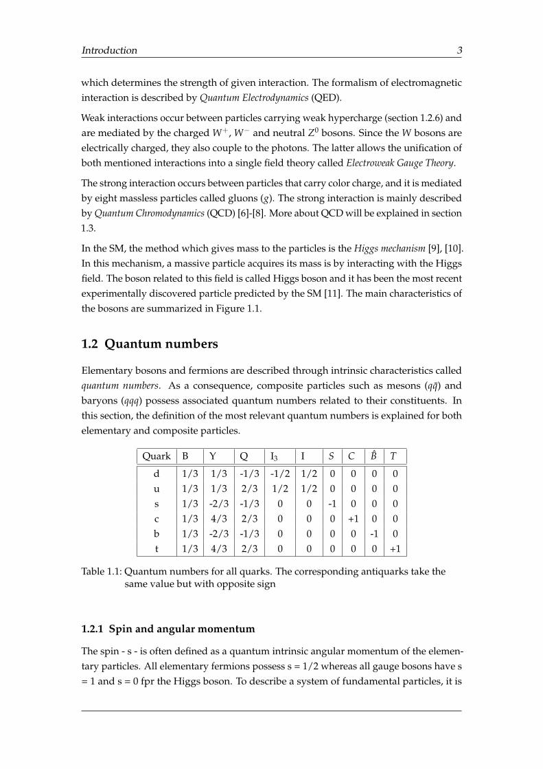
Table 1.1: Quantum numbers for all quarks. . . . . . . . . . . . . . . . . . . . . . . 3
Table 3.1: Main properties of the involved particles in the pp→ Σ0 channel. . . . 26
Table 4.1: Optimal average luminosities L at pbeam = 1.5 GeV/c. . . . . . . . . . . 32Table 4.2: Optimal average luminosities L at pbeam = 5.5 GeV/c. . . . . . . . . . . 32
Table 6.1: Total reconstructed final state particles from simulation performed withpbeam = 1.771 GeV/c. . . . . . . . . . . . . . . . . . . . . . . . . . . . . . 57
Table 6.2: Total reconstructed final state particles from simulation performed withpbeam = 6 GeV/c. . . . . . . . . . . . . . . . . . . . . . . . . . . . . . . . . 57
Table 6.3: Angular coverage of the principal tracking devices at the Target andForward spectrometer at PANDA. . . . . . . . . . . . . . . . . . . . . . 58
Table 6.4: Angular coverage of the principal PID devices in the Target and Forwardspectrometers at PANDA. . . . . . . . . . . . . . . . . . . . . . . . . . . 58
Table 6.5: Angular acceptance and energy ranges of the calorimeter. . . . . . . . . 59Table 6.6: Number of photon candidates before and after energy cut in the CM
frame. . . . . . . . . . . . . . . . . . . . . . . . . . . . . . . . . . . . . . . 65Table 6.7: Number of photon candidates before and after energy cut in the CM
frame. . . . . . . . . . . . . . . . . . . . . . . . . . . . . . . . . . . . . . . 67Table 6.8: Λ and Λ pre-selection process, pbeam = 1.771 GeV/c. . . . . . . . . . . . 70Table 6.9: Λ and Λ pre-selection process, pbeam = 6 GeV/c. . . . . . . . . . . . . . 70
Table 7.1: First method of Σ0 selection, pbeam = 1.771 GeV/c. . . . . . . . . . . . . 75Table 7.2: Second method of Σ0 selection, pbeam = 1.771 GeV/c. . . . . . . . . . . . 77
Table 8.1: Size sample, cross-section and weighting factors for the signal andbackground channels, pbeam = 1.771 GeV/c. . . . . . . . . . . . . . . . . 82
Table 8.2: Σ0Λ channel reconstruction process, pbeam = 1.771 GeV/c. . . . . . . . . 82Table 8.3: Size sample, cross-section and weighting factors for the signal and
background channels, pbeam = 6 GeV/c. . . . . . . . . . . . . . . . . . . 86Table 8.4: Σ0Λ channel reconstruction process, pbeam = 6 GeV/c. . . . . . . . . . 87
Table 9.1: Final efficiencies for pbeam = 1.771 GeV/c. . . . . . . . . . . . . . . . . . 88Table 9.2: Final efficiencies for pbeam = 6 GeV/c. . . . . . . . . . . . . . . . . . . . 89Table 9.3: Final efficiencies for pbeam = 6 GeV/c. . . . . . . . . . . . . . . . . . . . 89Table 9.4: Final efficiencies for pbeam = 6 GeV/c. . . . . . . . . . . . . . . . . . . . 89

List of Tables IX
Table 9.5: Reconstruction rates Nrec[s−1], at pbeam = 1.5 GeV/c. . . . . . . . . . . . 90Table 9.6: Reconstruction rates Nrec[s−1], at pbeam = 5.5 GeV/c. . . . . . . . . . . . 91
List of Figures X
List of Figures
Figure 1.1: Fundamental particles within the Standard Model . . . . . . . . . . . 1Figure 1.2: Summary of measurements of αs as a function of the respective energy
scale Q. . . . . . . . . . . . . . . . . . . . . . . . . . . . . . . . . . . . 8Figure 1.3: The lightest mesons. . . . . . . . . . . . . . . . . . . . . . . . . . . . . 10Figure 1.4: The lightest baryons. . . . . . . . . . . . . . . . . . . . . . . . . . . . . 11
Figure 2.1: Diagram showing three momenta of the particles involved in a 1 +
2→ 3 + 4 reaction. . . . . . . . . . . . . . . . . . . . . . . . . . . . . . 15Figure 2.2: Cross-section diagram. . . . . . . . . . . . . . . . . . . . . . . . . . . 17
Figure 3.1: Collection of all the cross-section measurements for the pp → YYreaction. . . . . . . . . . . . . . . . . . . . . . . . . . . . . . . . . . . . 20
Figure 3.2: Hyperon-antihyperon production diagrams in quark picture (a) andmeson exchange picture (b) . . . . . . . . . . . . . . . . . . . . . . . . 20
Figure 3.3: CM reference system showing the pp→ Σ0Λ reaction. . . . . . . . . 21Figure 3.4: Differential cross-sections as a function of the scattering angle cosθ∗
for two measurements performed at pbeam = 1.726 GeV/c and 1.771GeV/c. . . . . . . . . . . . . . . . . . . . . . . . . . . . . . . . . . . . . 22
Figure 3.5: Differential cross-section comparison of pp→ Σ0Λ at three commonexcess energies ε. . . . . . . . . . . . . . . . . . . . . . . . . . . . . . . 23
Figure 3.6: Σ0Λ and ΛΛ channels differential cross-sections dσ/dt at pbeam = 6GeV/c. . . . . . . . . . . . . . . . . . . . . . . . . . . . . . . . . . . . . 24
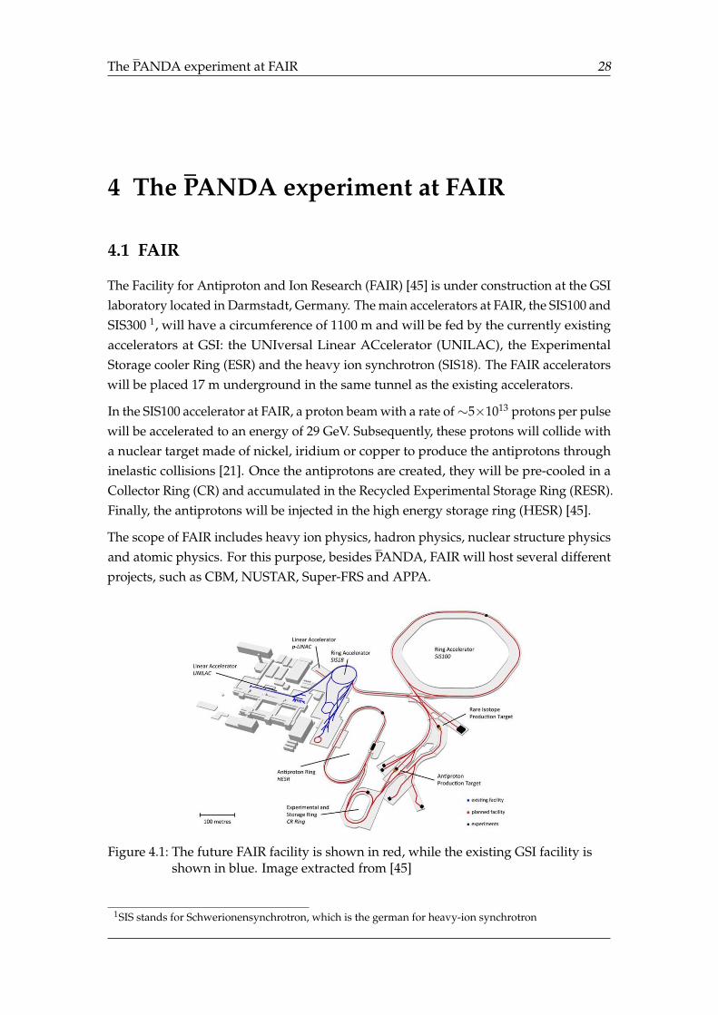
Figure 4.1: The future FAIR facility. . . . . . . . . . . . . . . . . . . . . . . . . . . 28Figure 4.2: The High Energy Storage Ring HESR layout. . . . . . . . . . . . . . . 29Figure 4.3: The PANDA detector layout. . . . . . . . . . . . . . . . . . . . . . . . 30Figure 4.4: The target spectrometer layout. The beam will run horizontally from
left to right and the target vertically from top to bottom. . . . . . . . 33Figure 4.5: The MVD layout. . . . . . . . . . . . . . . . . . . . . . . . . . . . . . . 35Figure 4.6: The Straw Tube Tracker (STT) layout. . . . . . . . . . . . . . . . . . . 36Figure 4.7: The DIRC detector layout. . . . . . . . . . . . . . . . . . . . . . . . . 37Figure 4.8: Barrel TOF detector layout. . . . . . . . . . . . . . . . . . . . . . . . . 38Figure 4.9: Barrel and forward endcap part of the EMC . . . . . . . . . . . . . . 39Figure 4.10: The muon system layout. . . . . . . . . . . . . . . . . . . . . . . . . . 40Figure 4.11: The Forward spectrometer (FS) layout . . . . . . . . . . . . . . . . . . 40Figure 4.12: The GEM planes layout. . . . . . . . . . . . . . . . . . . . . . . . . . . 41
List of Figures XI
Figure 4.13: The forward tracking stations. . . . . . . . . . . . . . . . . . . . . . . 42Figure 4.14: The FToF wall layout. . . . . . . . . . . . . . . . . . . . . . . . . . . . 43Figure 4.15: The forward calorimeter layout. . . . . . . . . . . . . . . . . . . . . . 44
Figure 5.1: Data flow in PandaRoot. . . . . . . . . . . . . . . . . . . . . . . . . . . 48
Figure 6.1: Inclusive study reaction scheme. . . . . . . . . . . . . . . . . . . . . . 54Figure 6.2: Exclusive study reaction scheme. . . . . . . . . . . . . . . . . . . . . . 55Figure 6.3: Generated (a) and reconstructed (b) Λ vertex position. . . . . . . . . 56Figure 6.4: Generated (a) and reconstructed (b) Λ vertex position. . . . . . . . . 56Figure 6.5: Diagram of the PANDA barrel part. . . . . . . . . . . . . . . . . . . . 58Figure 6.6: Angle vs energy ranges of generated(a) and reconstructed (b) an-
tiprotons. . . . . . . . . . . . . . . . . . . . . . . . . . . . . . . . . . . 59Figure 6.7: Angle vs energy ranges of generated(a) and reconstructed (b) protons. 60Figure 6.8: Angle vs energy ranges of generated(a) and reconstructed (b) π+. . 60Figure 6.9: Angle vs energy ranges of generated(a) and reconstructed (b) π−. . 61Figure 6.10: Angle vs energy ranges of generated(a) and reconstructed (b) an-
tiprotons. . . . . . . . . . . . . . . . . . . . . . . . . . . . . . . . . . . 61Figure 6.11: Angle vs energy ranges of generated(a) and reconstructed (b) protons. 62Figure 6.12: Angle vs energy ranges of generated(a) and reconstructed (b) π+. . 62Figure 6.13: Angle vs energy ranges of generated(a) and reconstructed (b) π−. . 63Figure 6.14: Angle range vs energy range for generated (a) and reconstructed
photons (b). . . . . . . . . . . . . . . . . . . . . . . . . . . . . . . . . . 64Figure 6.15: Range of energies of all the reconstructed photon candidates. . . . . 64Figure 6.16: Angle vs energy ranges of energy in the lab frame of all the photon
candidates after energy cut in the CM frame. . . . . . . . . . . . . . . 65Figure 6.17: Generated (a) and reconstructed (b) photons angle range vs energy
range. . . . . . . . . . . . . . . . . . . . . . . . . . . . . . . . . . . . . 66Figure 6.18: Range of energies of all the reconstructed photon candidates . . . . 66Figure 6.19: Reconstructed photons angle range vs energy ranges after cut on the
CM energy. . . . . . . . . . . . . . . . . . . . . . . . . . . . . . . . . . 67Figure 6.20: (a) Λ and (b) Λ probability distribution corresponding to the vertex
fit, pbeam = 1.771 GeV/c. . . . . . . . . . . . . . . . . . . . . . . . . . . 68Figure 6.21: (a) Λ and (b) Λ candidates invariant mass after vertex fit, pbeam = 1.771
GeV/c. . . . . . . . . . . . . . . . . . . . . . . . . . . . . . . . . . . . . 68Figure 6.22: (a) Λ and (b) Λ probability distribution corresponding to the vertex
fit, pbeam = 6 GeV/c. . . . . . . . . . . . . . . . . . . . . . . . . . . . . 69Figure 6.23: (a) Λ and (b) Λ candidates invariant mass after vertex fit, pbeam = 6
GeV/c. . . . . . . . . . . . . . . . . . . . . . . . . . . . . . . . . . . . . 69
Figure 7.1: (a) χ2 and (b) probability distribution corresponding to the vertex fiton the Λ candidates . . . . . . . . . . . . . . . . . . . . . . . . . . . . 72
List of Figures XII
Figure 7.2: Σ0 candidates Invariant mass after mass constraint, pbeam = 1.771 GeV/c. 72Figure 7.3: (a) χ2 and (b) distributions corresponding to the mass constraint on
Σ0 candidates, pbeam = 1.771 GeV/c. . . . . . . . . . . . . . . . . . . . 73Figure 7.4: Σ0 candidates invariant mass after mass constraint. . . . . . . . . . . 73Figure 7.5: Number of Σ0 candidates per event. . . . . . . . . . . . . . . . . . . . 74Figure 7.6: Σ0 candidates invariant mass after mass constraint, pbeam = 1.771 GeV/c 75Figure 7.7: Σ0 candidates invariant mass after final selection. . . . . . . . . . . . 75Figure 7.8: Σ0 candidates missing mass after mass constraint using mΣ0 = 1.192
GeV/c2. . . . . . . . . . . . . . . . . . . . . . . . . . . . . . . . . . . . 76Figure 7.9: Σ0 candidates missing mass after mass constraint using mΣ0 = 1.192
GeV/c2, pbeam = 1.771 GeV/c . . . . . . . . . . . . . . . . . . . . . . . 76
Figure 8.1: Σ0 candidates invariant mass at pbeam = 1.771 GeV/c . . . . . . . . . 79Figure 8.2: (a) χ2 and (b) probability distribution corresponding to vertex fit on
Λ candidates. . . . . . . . . . . . . . . . . . . . . . . . . . . . . . . . . 79Figure 8.3: Σ0 candidates invariant mass after final selection, pbeam = 1.771 GeV/c. 80Figure 8.4: Λ candidates invariant mass after final selection, pbeam = 1.771 GeV/c. 80Figure 8.5: Background and signal samples before last cut. . . . . . . . . . . . . 82Figure 8.6: (a) Σ0 candidates. (b)Photon energy boosted to the Σ0 rest frame,
pbeam = 6 GeV/c. . . . . . . . . . . . . . . . . . . . . . . . . . . . . . . 83Figure 8.7: Σ0 candidates invariant mass after boosted photon energy cut, pbeam
= 6 GeV/c. . . . . . . . . . . . . . . . . . . . . . . . . . . . . . . . . . . 84Figure 8.8: χ2 (a) and probability (b) distribution corresponding to Λ candidates
vertex fit. . . . . . . . . . . . . . . . . . . . . . . . . . . . . . . . . . . 85Figure 8.9: Σ0 candidates invariant mass after final selection,pbeam = 6 GeV/c. . 85Figure 8.10: Invariant mass Λ candidates after final selection, pbeam = 6 GeV/c. . 85Figure 8.11: Λ candidates decay vertex position. . . . . . . . . . . . . . . . . . . . 87Figure 8.12: Background and signal samples before last cut. . . . . . . . . . . . . 87
Introduction 1
1 Introduction
1.1 The Standard Model
The Standard Model of particles (SM) contains a description of the fundamental compo-nents of the Universe. It is a quantum field theory which elaborates a unified descriptionof the strong, weak, and electromagnetic forces in the language of quantum gauge-fieldtheories [1]. The latter means that in the SM, particles are related to field excitations i.e.waves. It is the quantization of these field excitations that gives rise to the existence ofthe elementary particles.
The SM has shown to be enormously successful in predicting and interpreting a widerange of phenomena: it includes all elementary particles that have been experimentallydiscovered. On the particle physics scale, gravitational effects are so small that they canbe neglected in this context.
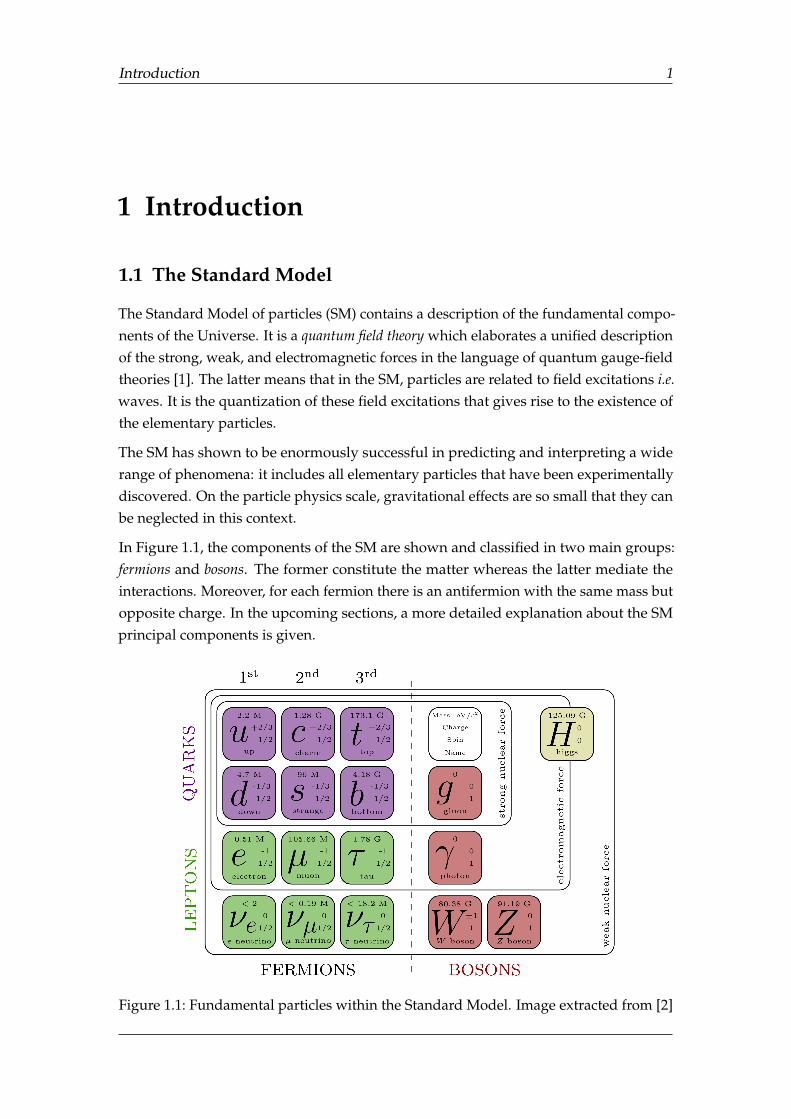
In Figure 1.1, the components of the SM are shown and classified in two main groups:fermions and bosons. The former constitute the matter whereas the latter mediate theinteractions. Moreover, for each fermion there is an antifermion with the same mass butopposite charge. In the upcoming sections, a more detailed explanation about the SMprincipal components is given.
Figure 1.1: Fundamental particles within the Standard Model. Image extracted from [2]
Introduction 2
1.1.1 Fermions
The fermions are half integer spin particles, which obey the Pauli exclusion principle.They are divided in two subgroups: leptons and quarks. The six known leptons interactelectromagnetically and weakly and can be arranged in three SU(2) doublets as shownat expression 1.1. Each doublet constitutes a charged lepton (top row) and its associatedneutrino (bottom row). (
e−
νe
),(
µ−
νµ
),(
τ−
ντ
)(1.1)
Quarks on the other hand, interact via electromagnetic, weak and strong force. In thesame way as leptons, the six different quark flavors are arranged in three SU(2) doubletsas expressed at 1.2. The main properties of quarks and leptons are summarized in Figure1.1. (
ud
),(
cs
),(
tb
)(1.2)
The combination of a quark and a lepton doublet give as a result a family or generationof fermions. There are three generations as shown in Figure 1.1, labeled 1st, 2nd and 3rd.Flavor transitions occur through weak interaction and are more probable within the samedoublet than between doublets. All the probabilities are given by the Cabibbo-KobayashiMaskawa (CKM) matrix [3], [4] which describes all the flavor-changing processes in theSM. The members of the 1st generation are lighter than the members of the remainingtwo. As a consequence, matter constituted by the second or third generation memberswill eventually decay into objects belonging to the 1st generation, and since there are nolighter fundamental particles to which these can decay, the first generation members arestable and constitute all the matter that surrounds us.
Due to strong interaction effects explained in section 1.3, quarks cannot be observedindividually in Nature, but only grouped into bound states called hadrons. Dependingon its internal composition, hadrons are classified as mesons or baryons. The formerconsists on quark-antiquark (qq) pairs, whereas the latter are three quarks (qqq) or threeantiquarks (qqq) combinations, in which case they are called antibaryons.
1.1.2 Bosons
The bosons are all integer spin particles. In particular, gauge bosons are responsible ofmediating the interactions among fermions. These are the photon γ, the gluons g, the W±
and the neutral Z0. The interactions described in the SM are characterized by differentranges and strengths: the electromagnetic force has infinite range, while the strong andweak interactions manifest at a scale of 10−15m and 10−18m [5] respectively. Moreover,all interactions are characterized by different types of charges e.g. electromagnetic chargeis associated with electromagnetic interaction, and its mediating bosons i.e. the masslessneutral photons, couple to electromagnetically charged particles. It is the coupling
Introduction 3
which determines the strength of given interaction. The formalism of electromagneticinteraction is described by Quantum Electrodynamics (QED).
Weak interactions occur between particles carrying weak hypercharge (section 1.2.6) andare mediated by the charged W+, W− and neutral Z0 bosons. Since the W bosons areelectrically charged, they also couple to the photons. The latter allows the unification ofboth mentioned interactions into a single field theory called Electroweak Gauge Theory.
The strong interaction occurs between particles that carry color charge, and it is mediatedby eight massless particles called gluons (g). The strong interaction is mainly describedby Quantum Chromodynamics (QCD) [6]-[8]. More about QCD will be explained in section1.3.
In the SM, the method which gives mass to the particles is the Higgs mechanism [9], [10].In this mechanism, a massive particle acquires its mass is by interacting with the Higgsfield. The boson related to this field is called Higgs boson and it has been the most recentexperimentally discovered particle predicted by the SM [11]. The main characteristics ofthe bosons are summarized in Figure 1.1.
1.2 Quantum numbers
Elementary bosons and fermions are described through intrinsic characteristics calledquantum numbers. As a consequence, composite particles such as mesons (qq) andbaryons (qqq) possess associated quantum numbers related to their constituents. Inthis section, the definition of the most relevant quantum numbers is explained for bothelementary and composite particles.
Quark B Y Q I3 I S C B T
d 1/3 1/3 -1/3 -1/2 1/2 0 0 0 0u 1/3 1/3 2/3 1/2 1/2 0 0 0 0s 1/3 -2/3 -1/3 0 0 -1 0 0 0c 1/3 4/3 2/3 0 0 0 +1 0 0b 1/3 -2/3 -1/3 0 0 0 0 -1 0t 1/3 4/3 2/3 0 0 0 0 0 +1
Table 1.1: Quantum numbers for all quarks. The corresponding antiquarks take thesame value but with opposite sign
1.2.1 Spin and angular momentum
The spin - s - is often defined as a quantum intrinsic angular momentum of the elemen-tary particles. All elementary fermions possess s = 1/2 whereas all gauge bosons have s= 1 and s = 0 fpr the Higgs boson. To describe a system of fundamental particles, it is
Introduction 4
convenient to define the total angular momentum J which is a quantity that relates thetotal spin of the system S with its total orbital angular momentum L as:
J = L + S (1.3)
Thus, the values that J can take go from J = |L− S| to J = |L + S|. Given its definition, Jdepends on the type of bound system to be described i.e. mesons or baryons.
If the quark and antiquark forming a meson have a spin value of sq and sq respectively,the total spin of the system has a value of S = sq + sq. If Sq and Sq are not aligned, thespin vectors add up to make a vector of length |S| = 0 with one spin projection (Sz = 0),and is referred to as the spin-0 singlet. If the spins are aligned then |S| = 1, with threespin projections (Sz = +1, Sz = 0, and Sz = -1) and is called the spin-1 triplet. For all cases,it follows that the J value depends on L, which in principle can take any integer value.
In the simple quark model, the total spin value of ground state baryons is given by S =Sq1 + Sq2 + Sq3 , with Sqi (i = 1,2,3) the spin of each individual quark. Thus the total spinvector has a length of either |S| = 1/2 or |S| = 3/2. To obtain the total baryon orbitalangular momentum, one first calculates the angular momentum between a pair of thequarks (L12) and then adds the orbital angular momentum (L3) of the third quark withrespect to L12, i.e. L = L12 + L3.
1.2.2 Parity
The parity (P) describes the response of a particle’s wave function to the sign inversionof its space coordinates: (x,y,z)→ (−x,−y,−z). If the wave function remains the same,the parity is even whereas if the sign changes, it is odd. A fermion and an antifermion hasalways opposite parity: by convention Pq = 1 for quarks, and as a consequence Pq = −1for antiquarks.
P is calculated differently for mesons and baryons. Keeping in mind that L is the orbitalangular momentum, mesons have parity PM given by
PM = PqPq(−1)L = (−1)L+1 (1.4)
whereas for baryons and antibaryons, the parity PB and PB is given respectively by
PB = Pq1 Pq2 Pq3(−1)L12(−1)L3 = (−1)L12+L3 = −PB (1.5)
For the case L = L12 = L3=0, the parity is by convention P = -1 for mesons and antibaryons,whereas P = 1 for baryons. Parity is a property conserved in strong and electromagneticinteractions but can be violated in weak interactions.
Introduction 5
1.2.3 Isospin
The similar neutron (udd) and proton (uud) mass, led to their classification as twostates of the same particle with different charges. As a consequence, the Isospin (I) wasintroduced as an SU(2) (approximate) symmetry obeyed by the strong interaction, wherethe two states are the u and d flavors. Hadrons can be organized in families called isospinmultiplets. Particles that constitute a multiplet have very similar mass values and thesame spin and parity, therefore the way to distinguish between them is through theircharge and the z-component of their isospin, denoted I3. The isospin is conserved instrong interactions but not in electromagnetic nor in weak interactions. It is defined as I= 1/2 for u and d quarks whereas it is I = 0 for the rest of the quarks. For a combinationof quarks, I3 is defined as the following
I3 =12(nu − nd) (1.6)
where nu and nd are the number of u and d quarks respectively. Detailed informationabout the mentioned multiplets will be explained in further sections.
The weak isospin is a quantum number parallel to the previously defined I, but associatedto the weak interaction. Weak isospin is usually denoted by T with third component T3.It is conserved in weak, electromagnetic and strong interactions.
1.2.4 Baryon number
The baryon number - B - is an additive quantum number conserved in all the SMinteractions. It is defined as
B =13(nq − nq) (1.7)
where nq and nq are the number of quarks and antiquarks respectively. All baryons haveB = 1, while B = -1 for antibaryons. For mesons on the other hand, B = 0.
1.2.5 Lepton number
The lepton number -L- relates the number of leptons and antileptons within a system. Lis additive, and its mathematical definition is given by:
L = nl − nl (1.8)
where nl is the number of leptons and nl is the number of antileptons. With the definitionshown in Equation 1.8, leptons have L = 1 whereas antileptons have L = -1. All non-leptonic particles have L = 0. Lepton number has to be conserved in the SM interactions.However, in models beyond the SM, L violation can occur e.g. in Majorana neutrinos[13].
Introduction 6
1.2.6 Hypercharge
The hypercharge - Y - is a quantum number related to the quark flavor. Y is defined as
Y = B + S + C + B + T (1.9)
where B is the baryon number, and S,C, B and T are associated with the quark flavordefined as in Table 1.2. The hypercharge is conserved in strong interactions but not inweak interactions. It can also be seen as the combination of isospin and flavor into asingle charge operator with the following definition:
I3 = Q− Y2
(1.10)
where Q denotes the electric charge. Y does not apply to leptons. In contrast, the weakhypercharge (YW) is a quantum number associated to the lepton number and that relatesthe electric charge and the third component of weak isospin (T3) in the following way:
T3 = Q +YW
2(1.11)
1.2.7 Charge conjugation
The charge conjugation denoted by the operator - C -, is a transformation that convertsa particle into its corresponding antiparticle. Electromagnetic charge, quark flavorand I3 change sign under this transformation. Mass, spin and magnetic moment thatremain unchanged. As a consequence, the electromagnetic and strong interactions areC-invariant whereas the weak interaction is not.
The quantum number associated with the charge conjugation transformation is deter-mined by its eigenvalues and is called the C-parity. Only neutral particles which aretheir own anti-particle can be C eigenstates i.e. the photon and mesons like the neutralπ0 or η. Denoting L the orbital angular momentum, the C-parity is defined as
C = (−1)L (1.12)
The C-parity is only relevant to neutral mesons with neutral-flavor quantum number [15].The combination of charge conjugation and parity is called CP-inversion. CP-symmetryis conserved in electromagnetic and strong interactions, but can be violated in weakinteractions. The latter was first observed in neutral K meson decays [12] and morerecently, the LHCb collaboration claimed to find evidence of CP violation in Λ0
b baryondecays [14].
Introduction 7
1.3 Quantum Chromodynamics
The theory of the strong interactions between quarks and gluons is called QuantumChromodynamics (QCD). It is a quantum field theory which studies the property as-sociated with strongly interacting objects: the color charge. There are three possiblecolor charges for quarks: red, blue and green, while the corresponding anticolors areassociated to antiquarks. Unlike the electromagnetically neutral photons, which don’tinteract with each other, gluons are not color neutral but carry color charge themselves.This means that interactions between gluons - self interactions - exist. As a consequence,QCD is a non-Abelian theory.
To get a better insight of the striking nature of the strong interaction, one can lookat its coupling αs. In both the electromagnetic and strong interactions, the potentialbetween two charged particles depends on the distance at which it is measured orequivalently, on the energy transferred (Q). In QED when two charged particles areseparated, the interaction strength between them decreases as the distance increases.This is a consequence of vacuum polarization which means that electron-positron pairsare created in the vacuum, producing an screening effect on the charge as the distancefrom it increases. The screening effect disappears as one gets closer to the charge. Thelatter is reflected in the QED running coupling αe which grows at small distances (largeQ) and decreases at large distances (small Q).
In contrast to QED, in QCD the vacuum creates both quark-antiquark pairs whichcreate an screening effect, and gluons which create an anti-screening effect. The latter isstronger as one moves away from the color charge. As a consequence, αs is stronger atlarge distances (small Q) and weaker at small distances (large Q).
The decreasing αs in the short range limit is called asymptotic freedom and it means thatquarks behave as free particles when the distance between them is very small. At thisrange, the coupling can be well studied by perturbative methods (pQCD) and in fact, ithas been widely explored and understood [15].
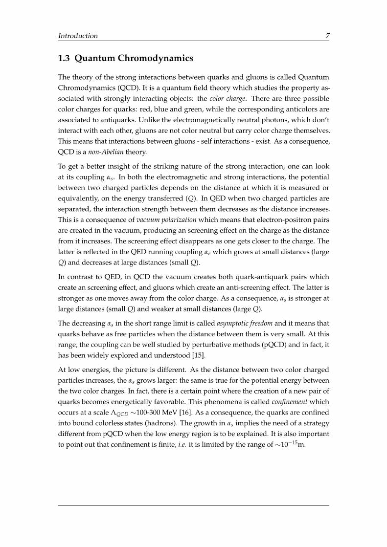
At low energies, the picture is different. As the distance between two color chargedparticles increases, the αs grows larger: the same is true for the potential energy betweenthe two color charges. In fact, there is a certain point where the creation of a new pair ofquarks becomes energetically favorable. This phenomena is called confinement whichoccurs at a scale ΛQCD ∼100-300 MeV [16]. As a consequence, the quarks are confinedinto bound colorless states (hadrons). The growth in αs implies the need of a strategydifferent from pQCD when the low energy region is to be explained. It is also importantto point out that confinement is finite, i.e. it is limited by the range of ∼10−15m.
Introduction 8
Figure 1.2: Summary of measurements of αs as a function of the respective energy scaleQ. Image extracted from [15]
The simplest way to achieve colorless states is through a quark-antiquark (color-anticolor)combination in a meson configuration, a combination of three quarks (blue-red-green) ina baryon configuration or three antiquarks (antired-antiblue-antigreen) in an antibaryonconfiguration. The most common hadrons are the nucleons, which are composed bythe lightest quarks u and d. Even though these are the constituents of the matter thatsurround us, they are not fully understood [17]-[19]. For instance, only about 2% of theirmass is generated by the afore-mentioned Higgs mechanism, while the rest is generateddynamically by the strong interaction. However, the exact mechanism is one of the openquestions in modern physics.
In Fig. 1.2, a summary of αs predictions together with experimental measurements isdisplayed. Even though a good agreement between theory and experiments is seen, ithas to be highlighted that the scale of the x-axis in Figure 1.2 only goes down to 1 GeV i.e.below this energy, pQCD breaks down and αs diverges. The fact that different strategieshave to be used to perform calculations at high energies and low energies calls for newinvestigations. In the energy scale at which αs diverges, several approaches such as latticeQCD and effective field theories have been adopted to explore the strong interactionobservables e.g. hadron masses, cross-sections, decay rates, etc. Even though thesemodels explain to some extent the experimental findings, neither of them can cover allobservables and one would like to have a coherent and calculable theory that describesthe interactions in the full energy domain. One of the challenges that QCD has to face toexplain the strong interaction at all ranges of energies are the different degrees of freedomthat have to be taken into account. Quarks and gluons are considered the degrees offreedom at high energies, whereas the hadrons perform this role at low energies. At theintermediate energy scales it remains unclear which are the proper degrees of freedomto take into account. The latter has motivated the study of a classification of baryonsnamed hyperons, which are explained at Section 1.4.3.
Introduction 9
1.4 The quark model
Since individual free quarks cannot be observed, hadrons become the direct object ofstudy and thus, cross-section (section 2.1.3) calculations and measurements of reactionsinvolving hadrons are one of the biggest source of information to study strong interactioneffects. The so called quark model provides a classification of hadrons in terms of some oftheir intrinsic properties.
In the quark model, hadrons are seen as composed by valence quarks, a sea made of virtualgluons and antiquark-quark pairs. The valence quarks determine the quantum numbersfor the possible bound states and their dynamical properties, e.g. the uud quarks withina proton. Therefore, the quark-gluon sea is usually not referred to when it comes todescribe a hadron composition. However it plays an important role in characterizing itselectric charge distribution and its magnetic moment [20].
In the quark model, hadrons are classified in hadrons multiplets under the assumption ofthe strong interaction SU(3) symmetry under flavor transformations [6], where the threeavailable states are the u, d and s flavors.
The spectroscopic notation JP, where J is the total angular momenta and P is the parity,is used to identify the principle features of the existing multiplets. The simple quarkmodel, which is explained in the following sections, includes all the experimentallyobserved hadrons. However, the model can be extended to include other combinationsof flavor contents and charges allowed by QCD. All states that are not included in thesimple quark model are called exotic hadrons.
1.4.1 Mesons
Mesons are bosons, meaning that their wave function has to be symmetric. This wavefunction is defined taking into account position, spin, flavor and color of the qq configu-ration:
ΨM = ψM(space)φM( f lavor)χM(spin)ξM(color) (1.13)
Taking into account the lightest quarks (u, d, s) and antiquarks (u,d, s), a meson-likeconfiguration can be represented as an SU(3) multiplet 3 and its complex conjugate 3respectively. This in written as the following:
3⊗ 3 = 1⊕ 8 (1.14)
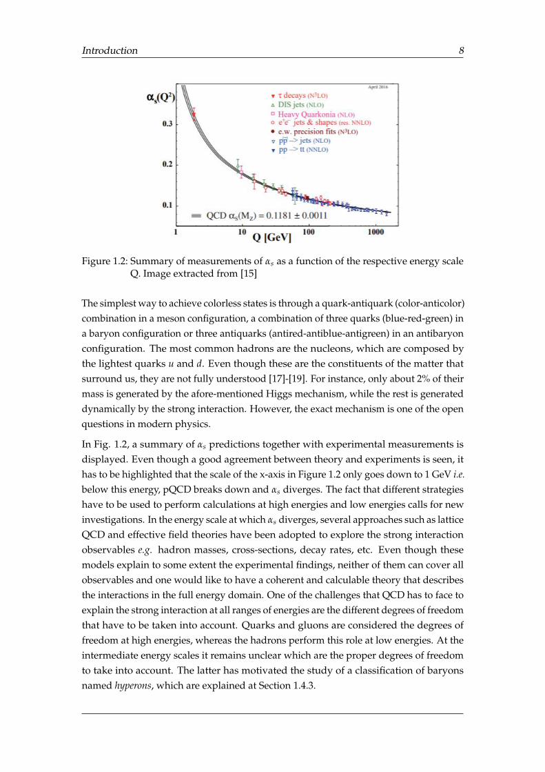
According to equation 1.14, nine states (nonet) are possible. If L = 0, the spin can be S =0 or S = 1 according to Equation 1.3, and implying odd parity from Equation 1.4. Thisresults in two possible arrangements called the pseudoscalar meson nonet (JP = 0−, Figure1.3 (a)) and the vector meson nonet (JP = 1−, Figure 1.3 (b)). These two nonets include allthe lightest mesons that have been experimentally observed for a given radial quantum
Introduction 10
number and with the same JP but different in charge, isospin and strangeness. In thisrepresentation, they are arranged according to their quantum numbers (Y, I3). Differentmembers of the same isospin multiplet lie on the same horizontal line.
Figure 1.3: The lightest mesons. Members of the same family with the same quantumnumbers are arranged in the same horizontal line
All nine mesons within a nonet would have the same mass if the flavor symmetry wereexact, and the model considers the symmetry breaking induced by the quark massdifferences.
1.4.2 Baryons
Since the baryons are fermions, the wave function needs to be antisymmetric. A generalwave function corresponding to a baryon is shown at equation 1.15.
ΨB = ψB(space)φB( f lavor)χB(spin)ξB(color) (1.15)
The color part is always antisymmetric under the exchange of two quarks, meaning thatonly those states in which ψ(space)φ( f lavor)χ(spin) form a symmetric wave functionare allowed. If the relative angular momentum is L = 0, the spatial part is symmetric. Thethree possible flavors the constituent quarks can take are represented as SU(3) triplets,and in group theory formalism, the possible flavor states are given by the following [21]:
3⊗ 3⊗ 3 = 10S ⊕ 8MS ⊕ 8MA ⊕ 1A (1.16)
On the other hand, the possible spin states for the quarks can be represented as threeSU(2) spin multiplets
2⊗ 2⊗ 2 = 4S ⊕ 2MS ⊕ 2MA (1.17)
The subindex S/A denote the symmetric/antisymmetric nature of the wave-functionunder the interchange of any two quarks, whereas MA/MS denote mixed symmetry/an-tisymmetry under the interchange of the first two quarks. The desired symmetric wave
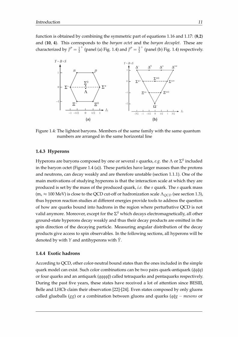
Introduction 11
function is obtained by combining the symmetric part of equations 1.16 and 1.17: (8,2)and (10, 4). This corresponds to the baryon octet and the baryon decuplet. These arecharacterized by JP = 1
2+
(panel (a) Fig. 1.4) and JP = 32+ (panel (b) Fig. 1.4) respectively.
Figure 1.4: The lightest baryons. Members of the same family with the same quantumnumbers are arranged in the same horizontal line
1.4.3 Hyperons
Hyperons are baryons composed by one or several s quarks, e.g. the Λ or Σ0 includedin the baryon octet (Figure 1.4 (a)). These particles have larger masses than the protonsand neutrons, can decay weakly and are therefore unstable (section 1.1.1). One of themain motivations of studying hyperons is that the interaction scale at which they areproduced is set by the mass of the produced quark, i.e. the s quark. The s quark mass(ms ≈ 100 MeV) is close to the QCD cut-off or hadronization scale ΛQCD (see section 1.3),thus hyperon reaction studies at different energies provide tools to address the questionof how are quarks bound into hadrons in the region where perturbative QCD is notvalid anymore. Moreover, except for the Σ0 which decays electromagnetically, all otherground-state hyperons decay weakly and thus their decay products are emitted in thespin direction of the decaying particle. Measuring angular distribution of the decayproducts give access to spin observables. In the following sections, all hyperons will bedenoted by with Y and antihyperons with Y.
1.4.4 Exotic hadrons
According to QCD, other color-neutral bound states than the ones included in the simplequark model can exist. Such color combinations can be two pairs quark-antiquark (qqqq)or four quarks and an antiquark (qqqqq) called tetraquarks and pentaquarks respectively.During the past five years, these states have received a lot of attention since BESIII,Belle and LHCb claim their observation [22]-[24]. Even states composed by only gluonscalled glueballs (gg) or a combination between gluons and quarks (qqg − mesons or

Introduction 12
qqqg− baryons) have been predicted, though not unambiguously identified. Despite therecent findings, these states are still referred to as exotic.
Formalism 13
2 Formalism
2.1 Relativistic kinematics
To describe a reaction in particle physics, calculations are performed using mathematicaltools called four-vectors. Its covariant components are denoted by a superscript, such thata covariant four-vector is written in the following way:
xµ = (x0, x1, x2, x3) = (ct, x,y,z) (2.1)
on the other hand, a contravariant four-vector is characterized by subscripts and it isdefined as:
xµ = (x0, x1, x2, x3) = (ct,−x,−y,−z) (2.2)
The metric tensor in the four-vector space denoted as gµν, is defined as a diagonal matrixwhose contravariant elements coincide with its covariant elements such that:
gµν = diag(1,−1,−1,−1) = gµν (2.3)
The scalar product between two four-vectors is a Lorentz invariant, and it is definedanalogously to a conventional three-vector scalar product, except that it always occursbetween a covariant and a contravariant four-vector. If x and y are two four-vectors, theirscalar product is given by
x · y = xµyµ = x0y0 + x1y1 + x2y2 + x3y3 (2.4)
the double appearance of the µ index in equation 2.4 denotes summation over all equalindices, and the minus signs are attributed to the non-Euclidean nature of the four-vectorspace.
The square of a four-vector given by x2 = x · x = xµxµ, is said to be time-like if x2 > 0, light-like if x2 = 0 and space-like if x2 < 0. For a particle with mass m, energy E and classicalthree-momentum ~p = (p1, p2, p3), its energy-momentum covariant four-momentum isdefined as:
pµ = (p0, p1, p2, p3) = (E,~p) (2.5)
The corresponding invariant 1 square is1Invariant due to its scalar nature.
Formalism 14
pµ pµ = E2 − |~p|2 = m2 (2.6)
where natural units (c = h = 1) in the equivalence between energy and mass E2 =
m2 + ~p2 has been used. From now on, natural units are adopted. The velocity of suchparticle is defined as ~p = γm~v and thus the relativistic factor γ is written as:
γ = (1− v2)−1/2 (2.7)
Combining equations 2.7 and 2.6, the following equations are obtained:
γ = E/m ~v = ~p/E (2.8)
which are commonly used in relativistic kinematics calculations. To write a four-momentum equation involving an initial and a final state, conservation of energy andmomentum have to be considered. In a system of n particles, the total energy andthree-momenta are given by
ETotal =n
∑i=0
Ei, ~pTotal =n
∑i=0
~pi (2.9)
this means that the total four-momentum of a system is given by
pTotalµ = (
n
∑i=0
Ei,n
∑i=0
~pi) (2.10)
Relativistic kinematics calculations can be performed in different reference frames andfour-vectors offer a convenient way to describe reactions and decays.
2.1.1 Two-body reaction
In particle physics, two-body reactions of the form 1 + 2→ 3 + 4 can be carried outin two scenarios: a beam impinging on a fixed target or two colliding beams. To start thedescription of the reaction in terms of relativistic kinematics, one has first to choosethe reference frame. The most commonly used are referred to as the laboratory frame(Lab) and the center-of-mass frame (CM). The Lab system is where the measurements areperformed i.e. the detector system. The CM is defined as the system where the totalthree-momentum is zero, i.e. ~pTotal = 0.
Formalism 15
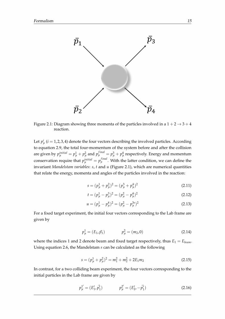
Figure 2.1: Diagram showing three momenta of the particles involved in a 1 + 2→ 3 + 4reaction.
Let piµ (i = 1,2,3,4) denote the four vectors describing the involved particles. According
to equation 2.9, the total four-momentum of the system before and after the collisionare given by pinitial
µ = p1µ + p2
µ and p f inalµ = p3
µ + p4µ respectively. Energy and momentum
conservation require that pinitialµ = p f inal
µ . With the latter condition, we can define theinvariant Mandelstam variables: s, t and u (Figure 2.1), which are numerical quantitiesthat relate the energy, momenta and angles of the particles involved in the reaction:
s = (p1µ + p2
µ)2 = (p3
µ + p4µ)
2 (2.11)
t = (p1µ − p3
µ)2 = (p2
µ − p4µ)
2 (2.12)
u = (p1µ − p4
µ)2 = (p2
µ − p3sµ )2 (2.13)
For a fixed target experiment, the initial four vectors corresponding to the Lab frame aregiven by
p1µ = (E1, ~p1) p2
µ = (m2,0) (2.14)
where the indices 1 and 2 denote beam and fixed target respectively, thus E1 = Ebeam.Using equation 2.6, the Mandelstam s can be calculated as the following
s = (p1µ + p2
µ)2 = m2
1 + m22 + 2E1m2 (2.15)
In contrast, for a two colliding beam experiment, the four vectors corresponding to theinitial particles in the Lab frame are given by
p1′µ = (E′1, ~p′1) p2′
µ = (E′2,−~p′1) (2.16)
Formalism 16
where particles 1 and 2 correspond to the two beams. In this case, the invariant quantitys is calculated the following
s = (p′µ1+ p′µ2
)2 = (E′1 + E′2)2 = (ECM)2 (2.17)
It is important to note that in this second case, since ~pTotal = 0, the Lab frame and theCM frame coincide. Moreover, according to equation 2.17, the total energy in the CMframe is given by ECM =
√s, which is often referred to as the available energy for the
reaction.
Sometimes in experiments where two body reactions are carried out, only one of thefinal particles is detected while the other one remains unknown. The correspondingreaction is written as
1 + 2→ 3 + X (2.18)
where X denotes the unmeasured particle. The identification of particle X is achievedby means of relativistic kinematics calculations. Four-momentum conservation dictatesthat the missing four-momentum i.e. belonging to the unmeasured particle, is given by
pXµ = p1
µ + p2µ − p3
µ (2.19)
Using Equation 2.6, it is possible to get the missing particle´s mass from Equation 2.19as:
pXµ pµX = m2
X = (p1µ + p2
µ − p3µ)(pµ1 + pµ2 − pµ3) (2.20)
From Equation 2.20, the mass of the unknown particle mX, can be written in terms ofthe known information and given that it is an invariant quantity, its calculation can bedeveloped in any of the reference frames.
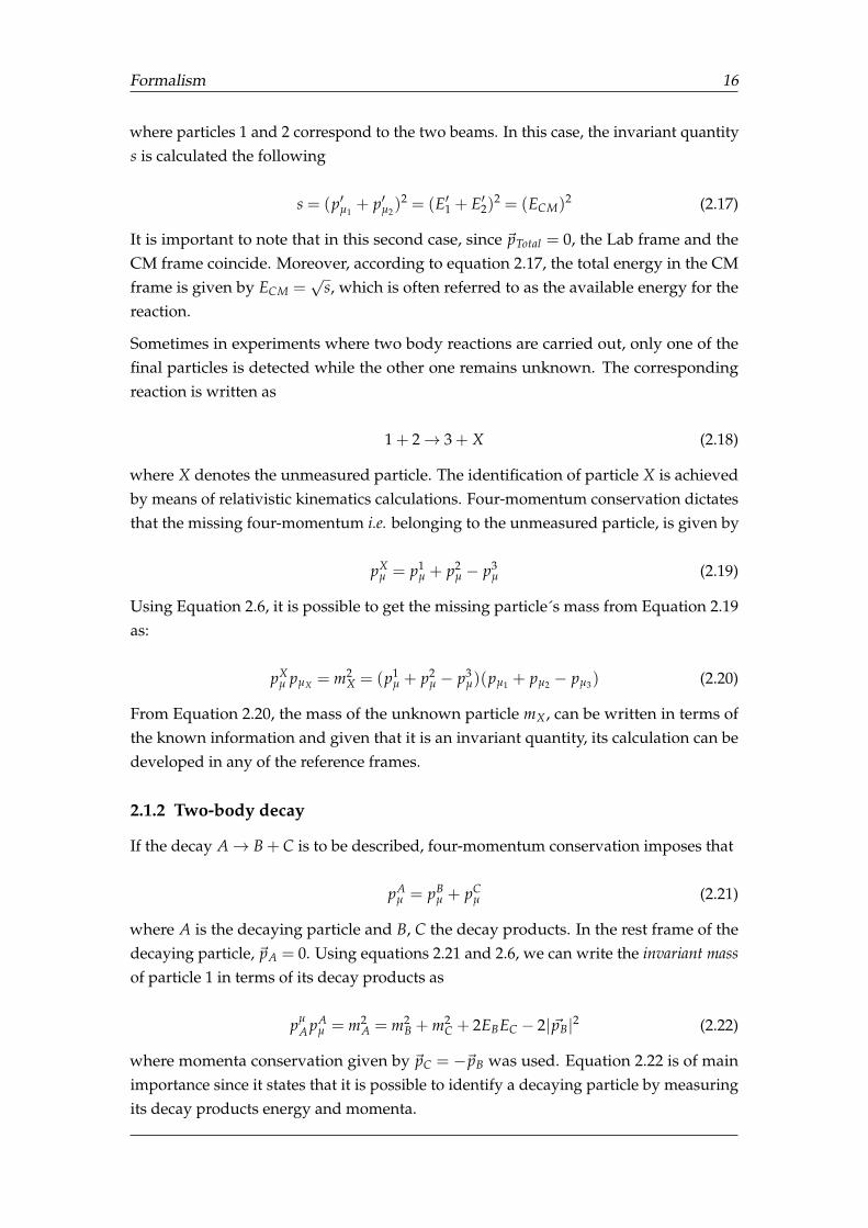
2.1.2 Two-body decay
If the decay A→ B + C is to be described, four-momentum conservation imposes that
pAµ = pB
µ + pCµ (2.21)
where A is the decaying particle and B, C the decay products. In the rest frame of thedecaying particle, ~pA = 0. Using equations 2.21 and 2.6, we can write the invariant massof particle 1 in terms of its decay products as
pµA pA
µ = m2A = m2
B + m2C + 2EBEC − 2|~pB|2 (2.22)
where momenta conservation given by ~pC = −~pB was used. Equation 2.22 is of mainimportance since it states that it is possible to identify a decaying particle by measuringits decay products energy and momenta.
Formalism 17
The distance the particle A travels before it decays can be calculated by means of itsmean-life τA using the relation LA = τAv, where v denotes its velocity. Using equations2.7 and 2.8, the distance can be re-written as
LA = τc
√1−
m2A
E2A
(2.23)
The distance LA depends on how much momentum the outgoing particle has. Hyperonscan travel from centimeters to meters depending on the experiment: at COMPASSat CERN, hyperons can travel several meters whereas at BESIII in Beijing, China, thedistances go from 0 to 3 cm. At PANDA it is envisaged that hyperons will travel from 1to 100 cm. The relatively long distances that hyperons can travel can be considered anadvantage since they are well distinguished from the interaction point. Nevertheless, italso represents a challenge since tracking devices are usually not designed to reconstructtracks which are not being generated at the interaction point.
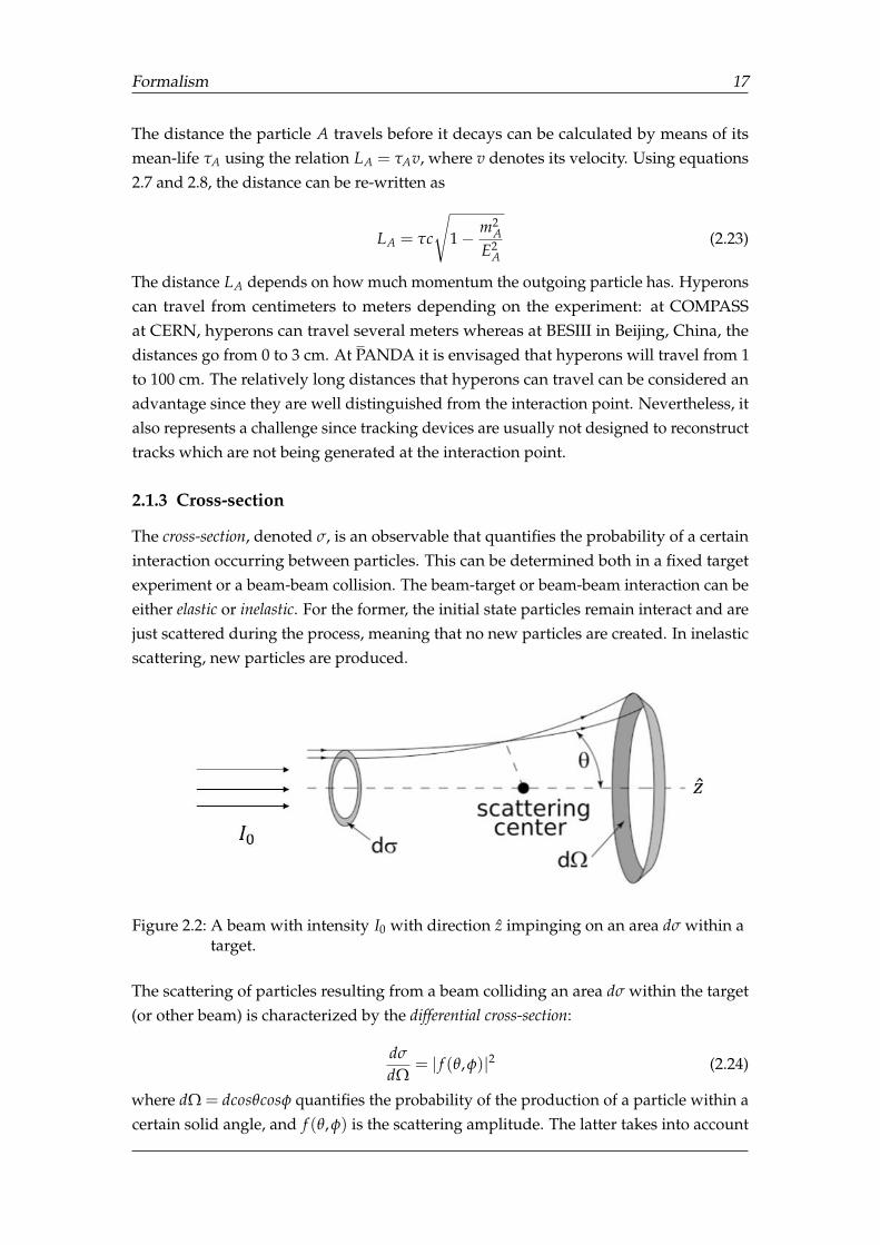
2.1.3 Cross-section
The cross-section, denoted σ, is an observable that quantifies the probability of a certaininteraction occurring between particles. This can be determined both in a fixed targetexperiment or a beam-beam collision. The beam-target or beam-beam interaction can beeither elastic or inelastic. For the former, the initial state particles remain interact and arejust scattered during the process, meaning that no new particles are created. In inelasticscattering, new particles are produced.
Figure 2.2: A beam with intensity I0 with direction z impinging on an area dσ within atarget.
The scattering of particles resulting from a beam colliding an area dσ within the target(or other beam) is characterized by the differential cross-section:
dσ
dΩ= | f (θ,φ)|2 (2.24)
where dΩ = dcosθcosφ quantifies the probability of the production of a particle within acertain solid angle, and f (θ,φ) is the scattering amplitude. The latter takes into account
Formalism 18
the structure of the particles involved, their energy and it is formally defined as theprobability amplitude of the outgoing spherical wave, relative to the incoming planewave in the scattering process [25]. The total cross-section is given by the integral of thedifferential cross-section over the full range of solid angle:
σ =∫ dσ
dΩdΩ =
∫| f (θ,φ)|2dΩ (2.25)
What is measured in an experiment is generally the number of particles going in a certaindirection. From that, the cross-section can be calculated provided that experimentalparameters such as background, luminosity (L) , detector efficiency (ε) and detector acceptance(A) are known. These quantities are related as
σ =N − B
L · ε · A (2.26)
there, σ is defined in units of area, whereas L can be seen as the rate of particles frombeam an target, per unit area that are brought so close together that they can interact.This number depends on the run time, target thickness and beam intensity. The efficiencymeasures a detector’s capability of finding objects which have passed through it, and itis defined as the fraction of recorded particles that fulfill certain selection criteria:
ε =Naccepted
Nrecorded(2.27)
The acceptance refers to the geometrical volume that the detector covers. In a situationwhere the particles incoming to the detector are isotropically distributed, A is defined as
A =Ω4π
(2.28)
where Ω is the full solid angle. It is customary to study and m easure the efficiency withthe acceptance and still denote it efficiency.
The pp→ Σ0Λ reaction 19
3 The pp→ Σ0Λ reaction
One of the physics topics that will be addressed at PANDA is strange hyperon produc-tion through pp→ YY reactions. The purpose of this chapter is to recall the generalmotivation to study this type of reactions, and to collect information that has beenlearned in previous measurements that will be useful for this work. Moreover, thespecific characteristics of the particles involved in the Σ0Λ channel are summarized, andsome kinematic calculations based on chapter 2.1 are performed.
3.1 General Motivation
As previously mentioned, hadronic reactions give information about the energy regioncorresponding to the mass of the produced quarks. This means that when a strange quarkis created (ms ∼ 100 MeV), the confinement domain will be probed. Profound studies onhyperon production are important to give insight on strong interaction features at thenon-perturbative QCD scale. Moreover, spin observables and differential cross-sectionsin reactions such as pp→ ΛΛ, Σ0Λ and ΛΣ0, helps pinpointing the role of the spin instrong interaction processes.
So far, experimental and theoretical emphasis have been given to the pp→ ΛΛ reaction.As it can be seen in Figure 3.1, a large amount of cross-section measurements havebeen performed for to this reaction, and detailed studies have been achieved by severalexperiments, in particular PS185 at LEAR (CERN). In their studies, they managed toperform a complete spin decomposition of the reaction [26]. However, the existingtheoretical models lack of a complete spin dynamics description, and there are fewmodel predictions and data about other hyperons different from Λ.
The pp→ Σ0Λ reaction 20
0,01
0,1
1
10
100
1000
1,4 1,5 1,6 1,7 1,8 1,9 2 2,1
Momentum [GeV/c]2 4 6 8 10 12 14
Momentum [GeV/c]
σ[µ
b]pp → ΛΛ
→ ΛΣ 0 + c.c.
→ Σ− Σ +
→ Σ 0 Σ 0
→ Σ + Σ −
→ Ξ0 Ξ0
→ Ξ+ Ξ−
Λc ΛcΞΞ ΩΩΛΣ0 ΣΣΛΛ
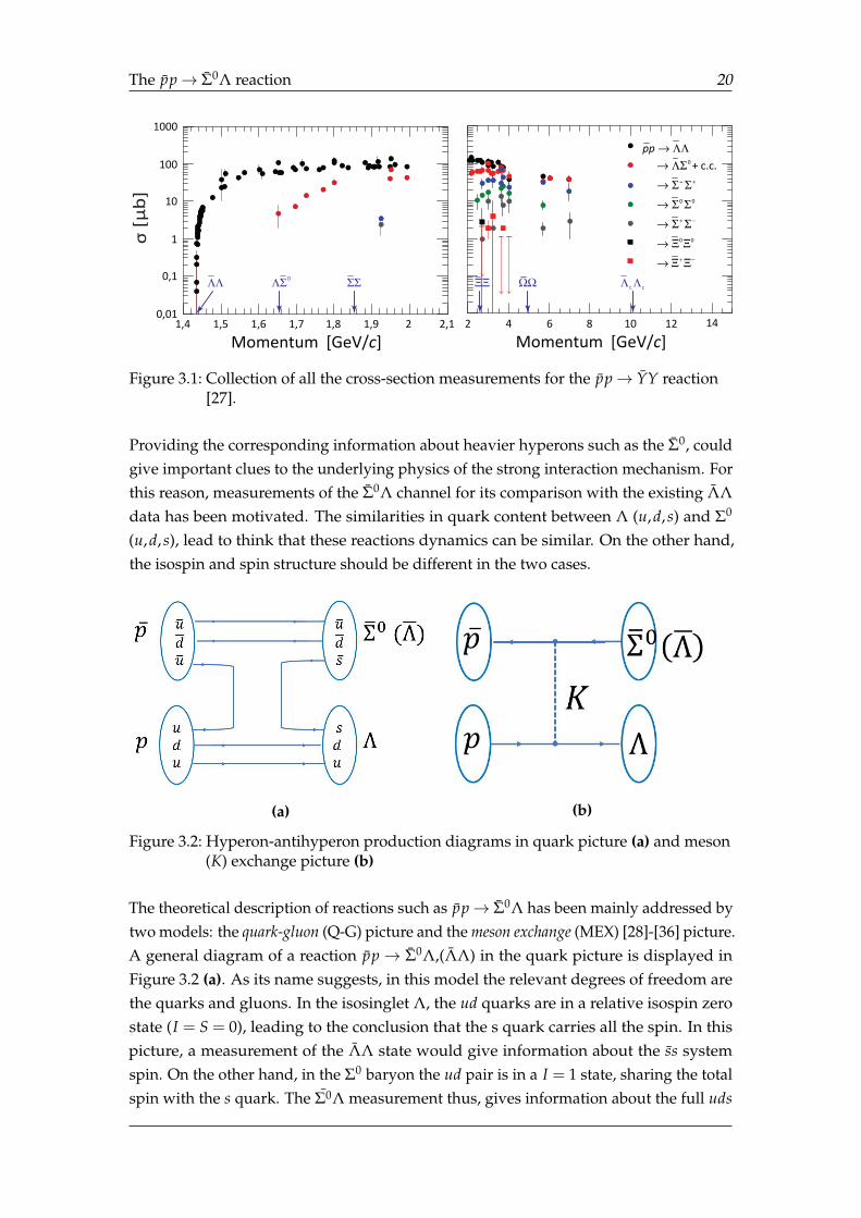
Figure 3.1: Collection of all the cross-section measurements for the pp→ YY reaction[27].
Providing the corresponding information about heavier hyperons such as the Σ0, couldgive important clues to the underlying physics of the strong interaction mechanism. Forthis reason, measurements of the Σ0Λ channel for its comparison with the existing ΛΛdata has been motivated. The similarities in quark content between Λ (u,d, s) and Σ0
(u,d, s), lead to think that these reactions dynamics can be similar. On the other hand,the isospin and spin structure should be different in the two cases.
(a) (b)
Figure 3.2: Hyperon-antihyperon production diagrams in quark picture (a) and meson(K) exchange picture (b)
The theoretical description of reactions such as pp→ Σ0Λ has been mainly addressed bytwo models: the quark-gluon (Q-G) picture and the meson exchange (MEX) [28]-[36] picture.A general diagram of a reaction pp→ Σ0Λ,(ΛΛ) in the quark picture is displayed inFigure 3.2 (a). As its name suggests, in this model the relevant degrees of freedom arethe quarks and gluons. In the isosinglet Λ, the ud quarks are in a relative isospin zerostate (I = S = 0), leading to the conclusion that the s quark carries all the spin. In thispicture, a measurement of the ΛΛ state would give information about the ss systemspin. On the other hand, in the Σ0 baryon the ud pair is in a I = 1 state, sharing the totalspin with the s quark. The Σ0Λ measurement thus, gives information about the full uds
The pp→ Σ0Λ reaction 21
system [39] and how the spin is distributed among the hyperon constituents. For thesereasons, the comparison between the channels in the Q-G picture provides informationabout the isospin dependence of the production mechanism.
In the MEX model (Figure 3.2 (b)), strangeness production is seen as a consequenceof the p and p exchanging a meson that contains one or more s quarks (K−meson forinstance). The latter means that the relevant degrees of freedom are mesons and baryons.In this case, the comparison between the ΛΛ and Σ0Λ channels gives information aboutthe couplings [28]-[36]. Predictions given by the MEX model establish that the strengthof the coupling in the Σ0 case is stronger than the Λ case. These and other strikingdifferences between the channels described in both models, encourages a comparisonbetween them.
It has been found that both models describe to some extent the experimental data sofar collected [26]. However, one would like to pinpoint which of these have a morecomplete description and in the long-run, provide guidance towards a new, morecoherent approach. To do this, more measurements are needed. It is of major importanceto understand the reactions and study its measurements feasibility. A simulation studyfor the pp→ ΛΛ has been performed for PANDA showing that spin observables can besuccessfully extracted (Ref [37]), the next step and focus of this thesis is to look at theΣ0Λ channel.
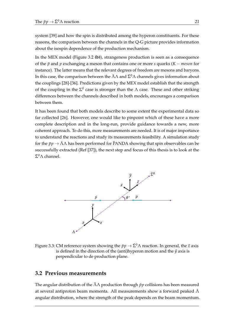
Figure 3.3: CM reference system showing the pp→ Σ0Λ reaction. In general, the z axisis defined in the direction of the (anti)hyperon motion and the y axis isperpendicular to de production plane.
3.2 Previous measurements
The angular distribution of the ΛΛ production through pp collisions has been measuredat several antiproton beam momenta. All measurements show a forward peaked Λangular distribution, where the strength of the peak depends on the beam momentum.
The pp→ Σ0Λ reaction 22
The corresponding differential cross-section measured at pbeam = 1.726 GeV/c and 1.771GeV/c are shown in Figure 3.4.
The first studies of the reaction pp→ Σ0Λ + c.c. reported by the PS185 collaborationat CERN, were performed at pbeam = 1.695 GeV/c. Even though the data sample wassmall, it was concluded that also here the antihyperon distribution was forwardly peakin the same way as in the ΛΛ case [38]. A later measurement at pbeam = 1.771 GeV/cwas performed by the same experiment. The sample consisted on approximately 1,500events for pp→ Σ0Λ and pp→ ΛΣ0 each. The total cross-sections reported, includingstatistical and systematic errors, were σ(Σ0Λ) = 10.85±0.27±0.48µb and σ(ΛΣ0) = 10.37± 0.24 ± 0.46 µb. The combined total cross-section was then obtained to be
σ( pp→ ΛΣ0 + c.c.) = 21.22± 0.36± 0.93µb (3.1)
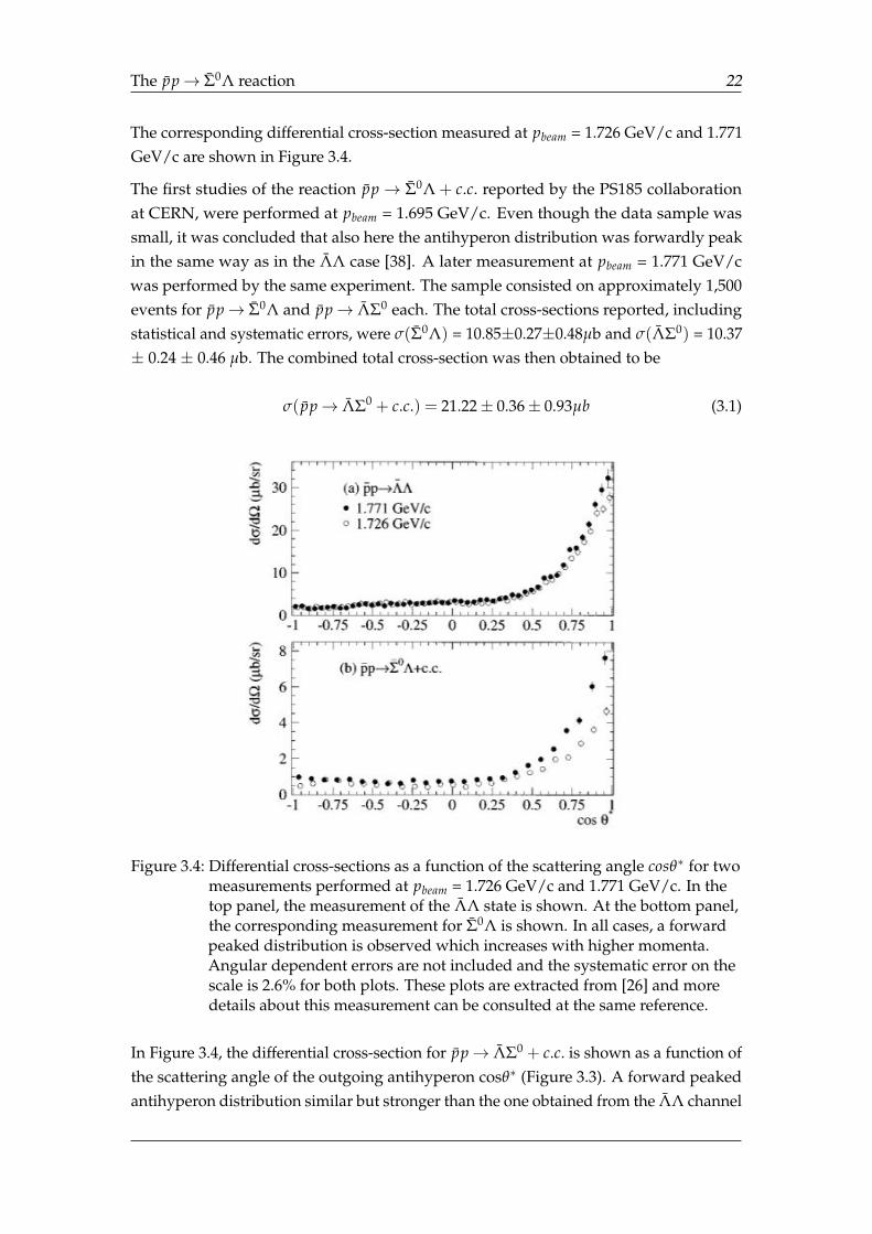
Figure 3.4: Differential cross-sections as a function of the scattering angle cosθ∗ for twomeasurements performed at pbeam = 1.726 GeV/c and 1.771 GeV/c. In thetop panel, the measurement of the ΛΛ state is shown. At the bottom panel,the corresponding measurement for Σ0Λ is shown. In all cases, a forwardpeaked distribution is observed which increases with higher momenta.Angular dependent errors are not included and the systematic error on thescale is 2.6% for both plots. These plots are extracted from [26] and moredetails about this measurement can be consulted at the same reference.
In Figure 3.4, the differential cross-section for pp→ ΛΣ0 + c.c. is shown as a function ofthe scattering angle of the outgoing antihyperon cosθ∗ (Figure 3.3). A forward peakedantihyperon distribution similar but stronger than the one obtained from the ΛΛ channel
The pp→ Σ0Λ reaction 23
measurements [39] is observed. A comparison between the differential cross-sections ofthe ΛΛ and ΛΣ0 + c.c. channels as a function of the reduced momentum t′ is shown inFigure 3.5. Setting t, p and q to be the four-momentum transfer squared, the incomingc.m. momentum and outgoing c.m. momentum respectively, the momentum transfer ofthe reaction depends on the scattering angle in the following way:
t′ = t− tmin = 2pq(cosθ∗ − 1) (3.2)
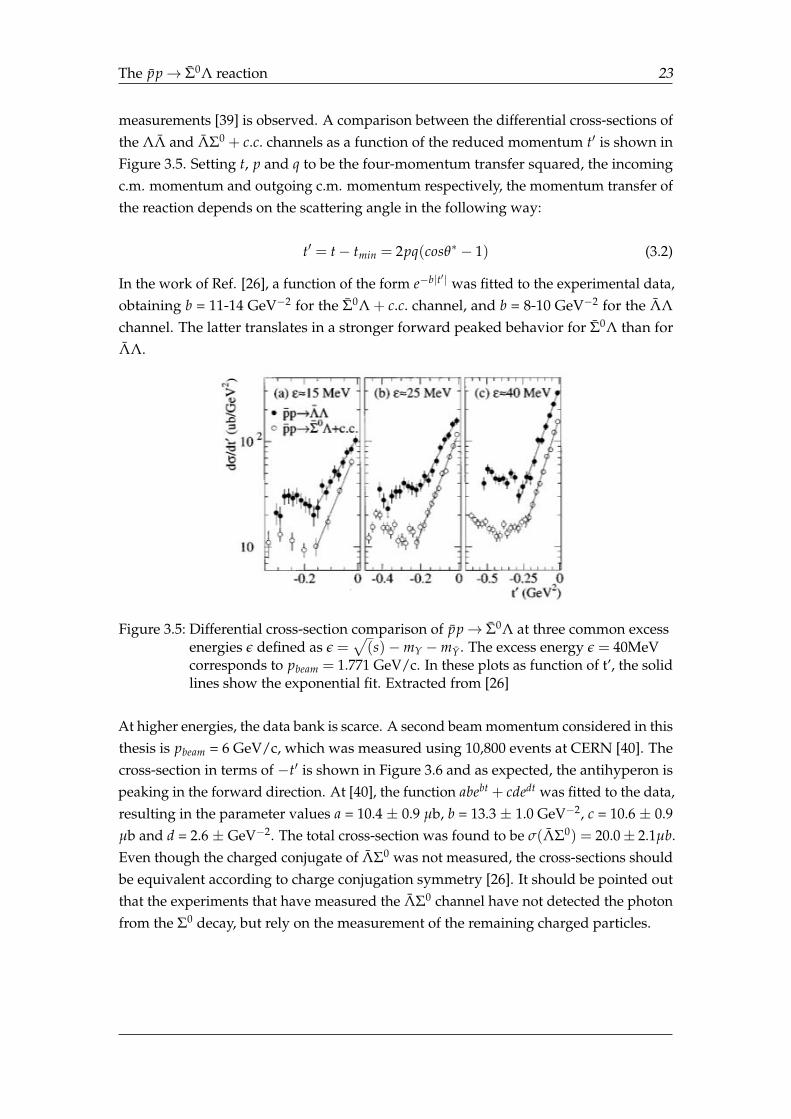
In the work of Ref. [26], a function of the form e−b|t′| was fitted to the experimental data,obtaining b = 11-14 GeV−2 for the Σ0Λ + c.c. channel, and b = 8-10 GeV−2 for the ΛΛchannel. The latter translates in a stronger forward peaked behavior for Σ0Λ than forΛΛ.
Figure 3.5: Differential cross-section comparison of pp→ Σ0Λ at three common excessenergies ε defined as ε =
√(s)−mY −mY. The excess energy ε = 40MeV
corresponds to pbeam = 1.771 GeV/c. In these plots as function of t’, the solidlines show the exponential fit. Extracted from [26]
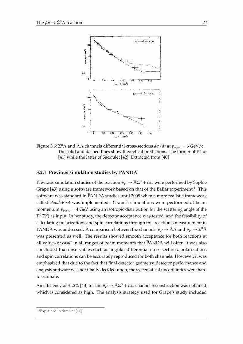
At higher energies, the data bank is scarce. A second beam momentum considered in thisthesis is pbeam = 6 GeV/c, which was measured using 10,800 events at CERN [40]. Thecross-section in terms of −t′ is shown in Figure 3.6 and as expected, the antihyperon ispeaking in the forward direction. At [40], the function abebt + cdedt was fitted to the data,resulting in the parameter values a = 10.4 ± 0.9 µb, b = 13.3 ± 1.0 GeV−2, c = 10.6 ± 0.9µb and d = 2.6 ± GeV−2. The total cross-section was found to be σ(ΛΣ0) = 20.0± 2.1µb.Even though the charged conjugate of ΛΣ0 was not measured, the cross-sections shouldbe equivalent according to charge conjugation symmetry [26]. It should be pointed outthat the experiments that have measured the ΛΣ0 channel have not detected the photonfrom the Σ0 decay, but rely on the measurement of the remaining charged particles.
The pp→ Σ0Λ reaction 24
Figure 3.6: Σ0Λ and ΛΛ channels differential cross-sections dσ/dt at pbeam = 6 GeV/c.The solid and dashed lines show theoretical predictions. The former of Plaut[41] while the latter of Sadoulet [42]. Extracted from [40]
3.2.1 Previous simulation studies by PANDA
Previous simulation studies of the reaction pp→ ΛΣ0 + c.c. were performed by SophieGrape [43] using a software framework based on that of the BaBar experiment 1. Thissoftware was standard in PANDA studies until 2008 when a more realistic frameworkcalled PandaRoot was implemented. Grape’s simulations were performed at beammomentum pbeam = 4 GeV using an isotropic distribution for the scattering angle of theΣ0(Σ0) as input. In her study, the detector acceptance was tested, and the feasibility ofcalculating polarizations and spin correlations through this reaction’s measurement inPANDA was addressed. A comparison between the channels pp→ ΛΛ and pp→ Σ0Λwas presented as well. The results showed smooth acceptance for both reactions atall values of cosθ∗ in all ranges of beam momenta that PANDA will offer. It was alsoconcluded that observables such as angular differential cross-sections, polarizationsand spin correlations can be accurately reproduced for both channels. However, it wasemphasized that due to the fact that final detector geometry, detector performance andanalysis software was not finally decided upon, the systematical uncertainties were hardto estimate.
An efficiency of 31.2% [43] for the pp→ ΛΣ0 + c.c. channel reconstruction was obtained,which is considered as high. The analysis strategy used for Grape’s study included
1Explained in detail at [44]
The pp→ Σ0Λ reaction 25
combining final state particles to reconstruct the full reaction and applying cuts basedon the kinematics of the initial pp system.
3.3 Motivation for this thesis
The present work aims to update the results presented by Sophie Grape with the morerealistic PandaRoot software. PandaRoot offers the most recent features of the detectordesign including inactive material such as supports. Furthermore, new analysis toolsare implemented which employs more realistic algorithms for pattern recognition andtracking (section 5).
The data sample has been weighted to angular distributions that have been observed inreal data: a forward peaked angular distribution parametrization based on the experi-mental data from PS185 described in Section 3.2 is used.
In this thesis we investigate the feasibility of measuring the pp→ Σ0Λ reaction withthe PANDA detector using two different approaches explained in detail in chapter 6.This is the first step to later on investigate if properties such as spin observables can beextracted for this channel. The beam momenta pbeam = 1.771 GeV/c and pbeam = 6 GeV/cused in this work, were chosen for easier comparison to previous measurements.
3.4 The pp system
There are different ways in which hyperon production can occur. In this work we areinterested in the features of the pp→ YY production mechanism, which is particularlyadvantageous since it is a highly symmetric process. Baryon number conservationalways requires the production of a Y1Y2 pair, giving the opportunity of comparingfundamental symmetries in antiparticle-particle observables. It is important to underlinethat Y1 and Y2 can be of different type as long as e.g. charge and flavor is conserved.
The isospin (I), total spin (J) and parity (P), the pp for the proton, have the followingvalues:
I(JP) =12
(12
)+
(3.3)
Taking into account the rules explained at section 1.2, the pp system has the followingquantum numbers:
• Isospin (I, I3) = (0,0) or (1,0)
• Spin (s) = 0 or 1
• Parity (P) = PpPp(−1)L = (−1)L+1
• Charge conjugation (C) = (−1)L+s
The pp→ Σ0Λ reaction 26
Moreover, the system has zero strangeness and charm. Even though these quantumnumbers constrains the possible final state particles from the pp annihilation, there is awide range of possible reactions, including the Σ0Λ channel.
3.5 Kinematic calculations
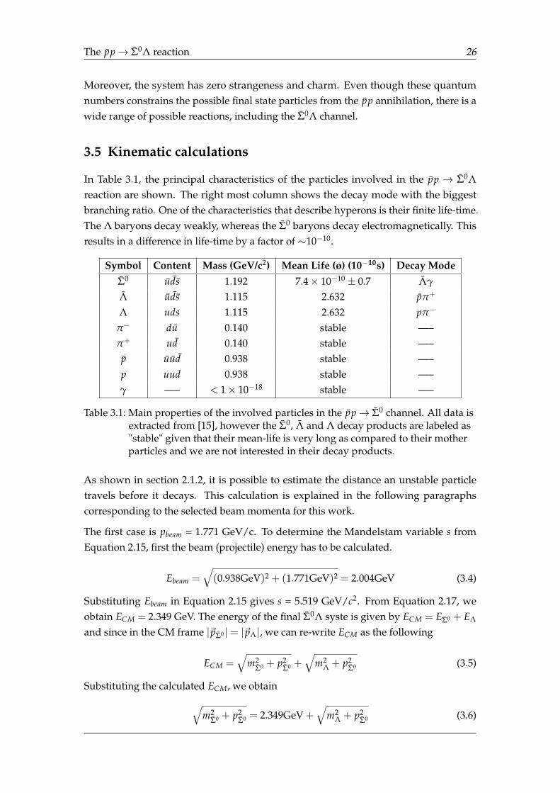
In Table 3.1, the principal characteristics of the particles involved in the pp → Σ0Λreaction are shown. The right most column shows the decay mode with the biggestbranching ratio. One of the characteristics that describe hyperons is their finite life-time.The Λ baryons decay weakly, whereas the Σ0 baryons decay electromagnetically. Thisresults in a difference in life-time by a factor of ∼10−10.
Symbol Content Mass (GeV/c2) Mean Life (ø) (10−10s) Decay ModeΣ0 uds 1.192 7.4× 10⁻¹⁰ ± 0.7 Λγ
Λ uds 1.115 2.632 pπ+
Λ uds 1.115 2.632 pπ−
π− du 0.140 stable —–π+ ud 0.140 stable —–p uud 0.938 stable —–p uud 0.938 stable —–γ —– < 1× 10⁻¹⁸ stable —–
Table 3.1: Main properties of the involved particles in the pp→ Σ0 channel. All data isextracted from [15], however the Σ0, Λ and Λ decay products are labeled as"stable" given that their mean-life is very long as compared to their motherparticles and we are not interested in their decay products.
As shown in section 2.1.2, it is possible to estimate the distance an unstable particletravels before it decays. This calculation is explained in the following paragraphscorresponding to the selected beam momenta for this work.
The first case is pbeam = 1.771 GeV/c. To determine the Mandelstam variable s fromEquation 2.15, first the beam (projectile) energy has to be calculated.
Ebeam =√(0.938GeV)2 + (1.771GeV)2 = 2.004GeV (3.4)
Substituting Ebeam in Equation 2.15 gives s = 5.519 GeV/c2. From Equation 2.17, weobtain ECM = 2.349 GeV. The energy of the final Σ0Λ syste is given by ECM = EΣ0 + EΛ
and since in the CM frame |~pΣ0 | = |~pΛ|, we can re-write ECM as the following
ECM =√
m2Σ0 + p2
Σ0 +√
m2Λ + p2
Σ0 (3.5)
Substituting the calculated ECM, we obtain√m2
Σ0 + p2Σ0 = 2.349GeV +
√m2
Λ + p2Σ0 (3.6)
The pp→ Σ0Λ reaction 27
Solving for pΣ0 , we get pΣ0 = 0.210 GeV/c. The Σ0 energy is then calculated throughEΣ0 =
√m2
Σ0 + p2Σ0 , giving a value of EΣ0 = 1.210 GeV. Finally, using the Σ0 mean life τΣ0
shown at Table 3.1, Equation 2.23 can be re-written as
LΣ0 = cτΣ0
√1−
m2Σ0
E2Σ0
= 3.815× 10⁻¹⁰ cm (3.7)
In the same way one can calculate the Λ hyperon decay length:
LΛ = cτΛ
√1−
m2Λ
E2Λ
= 4.45 cm (3.8)
From Equations 3.7 and 3.7, it is clear that the Σ0 baryons decay at a non-measurabledistance from the interaction point whereas the Λ baryons decay after a few centimeters.This is taken into account when designing detectors for accurate reconstruction of thechannels of interest.
For the case of higher momentum, pbeam = 6 GeV/c, s = 13.153 GeV2 and the correspond-ing ECM = 3.627 GeV. The decay lengths are calculated in the same way as the lowerbeam momentum giving a result of LΣ0 = 1.693 × 10⁻⁹ cm and LΛ = 6.12 cm, which arelonger than in the previous case as expected due to the higher momentum.
The PANDA experiment at FAIR 28
4 The PANDA experiment at FAIR
4.1 FAIR
The Facility for Antiproton and Ion Research (FAIR) [45] is under construction at the GSIlaboratory located in Darmstadt, Germany. The main accelerators at FAIR, the SIS100 andSIS300 1, will have a circumference of 1100 m and will be fed by the currently existingaccelerators at GSI: the UNIversal Linear ACcelerator (UNILAC), the ExperimentalStorage cooler Ring (ESR) and the heavy ion synchrotron (SIS18). The FAIR acceleratorswill be placed 17 m underground in the same tunnel as the existing accelerators.
In the SIS100 accelerator at FAIR, a proton beam with a rate of∼5×10¹³ protons per pulsewill be accelerated to an energy of 29 GeV. Subsequently, these protons will collide witha nuclear target made of nickel, iridium or copper to produce the antiprotons throughinelastic collisions [21]. Once the antiprotons are created, they will be pre-cooled in aCollector Ring (CR) and accumulated in the Recycled Experimental Storage Ring (RESR).Finally, the antiprotons will be injected in the high energy storage ring (HESR) [45].
The scope of FAIR includes heavy ion physics, hadron physics, nuclear structure physicsand atomic physics. For this purpose, besides PANDA, FAIR will host several differentprojects, such as CBM, NUSTAR, Super-FRS and APPA.
Figure 4.1: The future FAIR facility is shown in red, while the existing GSI facility isshown in blue. Image extracted from [45]
1SIS stands for Schwerionensynchrotron, which is the german for heavy-ion synchrotron
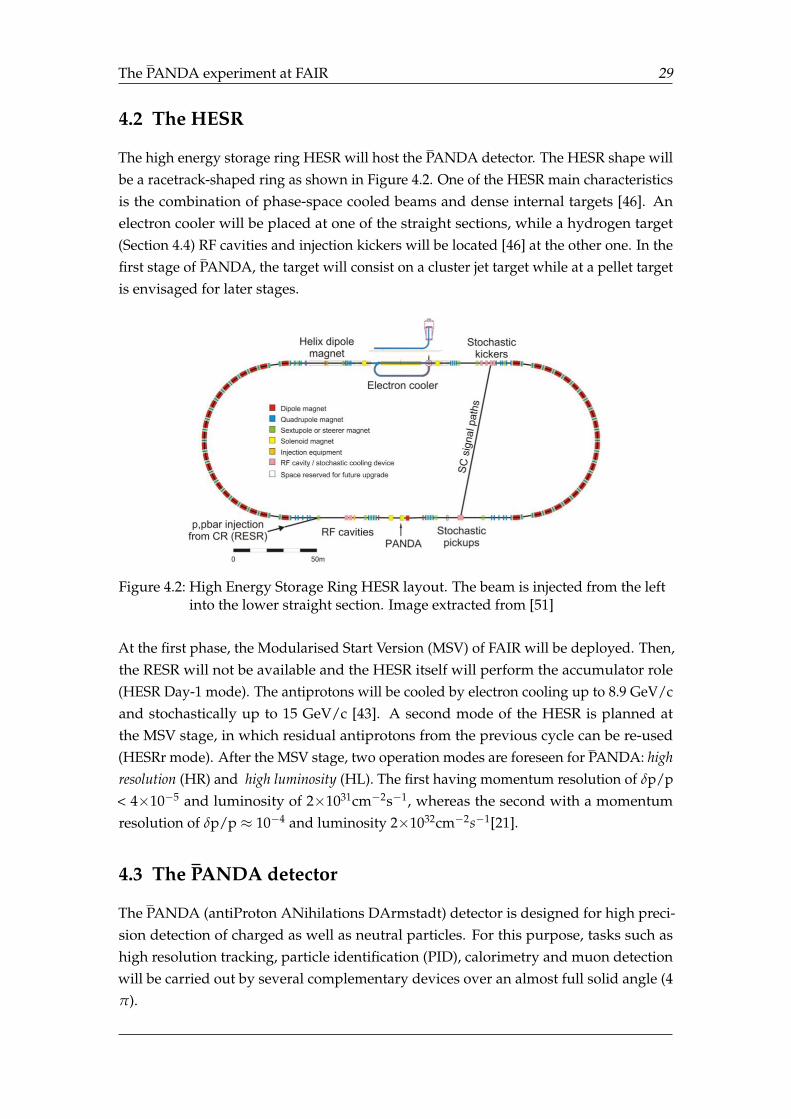
The PANDA experiment at FAIR 29
4.2 The HESR
The high energy storage ring HESR will host the PANDA detector. The HESR shape willbe a racetrack-shaped ring as shown in Figure 4.2. One of the HESR main characteristicsis the combination of phase-space cooled beams and dense internal targets [46]. Anelectron cooler will be placed at one of the straight sections, while a hydrogen target(Section 4.4) RF cavities and injection kickers will be located [46] at the other one. In thefirst stage of PANDA, the target will consist on a cluster jet target while at a pellet targetis envisaged for later stages.
Figure 4.2: High Energy Storage Ring HESR layout. The beam is injected from the leftinto the lower straight section. Image extracted from [51]
At the first phase, the Modularised Start Version (MSV) of FAIR will be deployed. Then,the RESR will not be available and the HESR itself will perform the accumulator role(HESR Day-1 mode). The antiprotons will be cooled by electron cooling up to 8.9 GeV/cand stochastically up to 15 GeV/c [43]. A second mode of the HESR is planned atthe MSV stage, in which residual antiprotons from the previous cycle can be re-used(HESRr mode). After the MSV stage, two operation modes are foreseen for PANDA: highresolution (HR) and high luminosity (HL). The first having momentum resolution of δp/p< 4×10⁻⁵ and luminosity of 2×1031cm−2s−1, whereas the second with a momentumresolution of δp/p ≈ 10−4 and luminosity 2×1032cm−2s−1[21].
4.3 The PANDA detector
The PANDA (antiProton ANihilations DArmstadt) detector is designed for high preci-sion detection of charged as well as neutral particles. For this purpose, tasks such ashigh resolution tracking, particle identification (PID), calorimetry and muon detectionwill be carried out by several complementary devices over an almost full solid angle (4π).
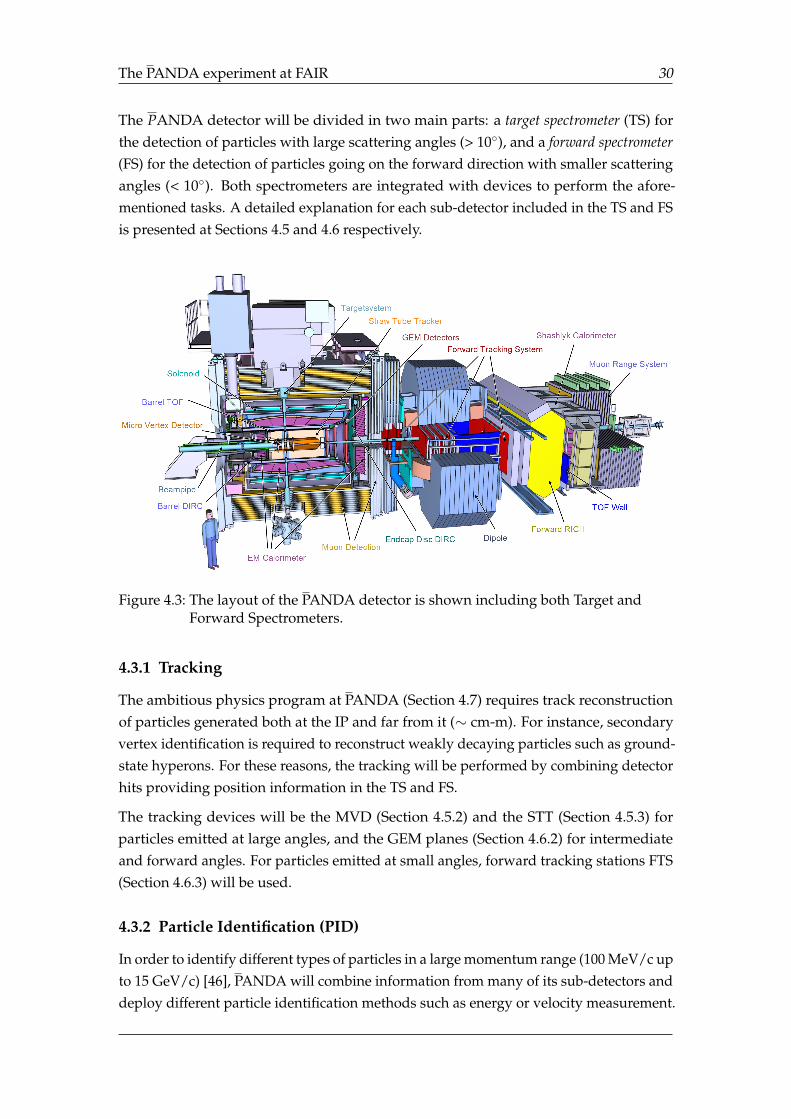
The PANDA experiment at FAIR 30
The PANDA detector will be divided in two main parts: a target spectrometer (TS) forthe detection of particles with large scattering angles (> 10), and a forward spectrometer(FS) for the detection of particles going on the forward direction with smaller scatteringangles (< 10). Both spectrometers are integrated with devices to perform the afore-mentioned tasks. A detailed explanation for each sub-detector included in the TS and FSis presented at Sections 4.5 and 4.6 respectively.
Figure 4.3: The layout of the PANDA detector is shown including both Target andForward Spectrometers.
4.3.1 Tracking
The ambitious physics program at PANDA (Section 4.7) requires track reconstructionof particles generated both at the IP and far from it (∼ cm-m). For instance, secondaryvertex identification is required to reconstruct weakly decaying particles such as ground-state hyperons. For these reasons, the tracking will be performed by combining detectorhits providing position information in the TS and FS.
The tracking devices will be the MVD (Section 4.5.2) and the STT (Section 4.5.3) forparticles emitted at large angles, and the GEM planes (Section 4.6.2) for intermediateand forward angles. For particles emitted at small angles, forward tracking stations FTS(Section 4.6.3) will be used.
4.3.2 Particle Identification (PID)
In order to identify different types of particles in a large momentum range (100 MeV/c upto 15 GeV/c) [46], PANDA will combine information from many of its sub-detectors anddeploy different particle identification methods such as energy or velocity measurement.
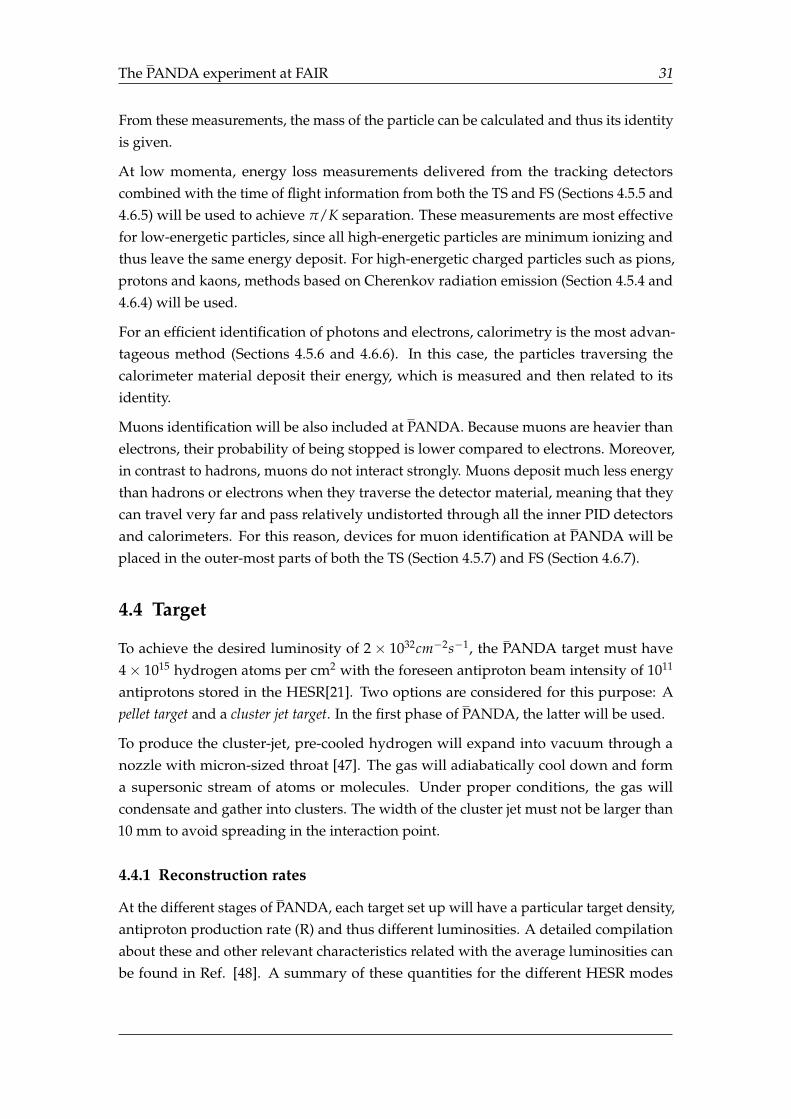
The PANDA experiment at FAIR 31
From these measurements, the mass of the particle can be calculated and thus its identityis given.
At low momenta, energy loss measurements delivered from the tracking detectorscombined with the time of flight information from both the TS and FS (Sections 4.5.5 and4.6.5) will be used to achieve π/K separation. These measurements are most effectivefor low-energetic particles, since all high-energetic particles are minimum ionizing andthus leave the same energy deposit. For high-energetic charged particles such as pions,protons and kaons, methods based on Cherenkov radiation emission (Section 4.5.4 and4.6.4) will be used.
For an efficient identification of photons and electrons, calorimetry is the most advan-tageous method (Sections 4.5.6 and 4.6.6). In this case, the particles traversing thecalorimeter material deposit their energy, which is measured and then related to itsidentity.
Muons identification will be also included at PANDA. Because muons are heavier thanelectrons, their probability of being stopped is lower compared to electrons. Moreover,in contrast to hadrons, muons do not interact strongly. Muons deposit much less energythan hadrons or electrons when they traverse the detector material, meaning that theycan travel very far and pass relatively undistorted through all the inner PID detectorsand calorimeters. For this reason, devices for muon identification at PANDA will beplaced in the outer-most parts of both the TS (Section 4.5.7) and FS (Section 4.6.7).
4.4 Target
To achieve the desired luminosity of 2× 1032cm−2s−1, the PANDA target must have4× 1015 hydrogen atoms per cm2 with the foreseen antiproton beam intensity of 1011
antiprotons stored in the HESR[21]. Two options are considered for this purpose: Apellet target and a cluster jet target. In the first phase of PANDA, the latter will be used.
To produce the cluster-jet, pre-cooled hydrogen will expand into vacuum through anozzle with micron-sized throat [47]. The gas will adiabatically cool down and forma supersonic stream of atoms or molecules. Under proper conditions, the gas willcondensate and gather into clusters. The width of the cluster jet must not be larger than10 mm to avoid spreading in the interaction point.
4.4.1 Reconstruction rates
At the different stages of PANDA, each target set up will have a particular target density,antiproton production rate (R) and thus different luminosities. A detailed compilationabout these and other relevant characteristics related with the average luminosities canbe found in Ref. [48]. A summary of these quantities for the different HESR modes
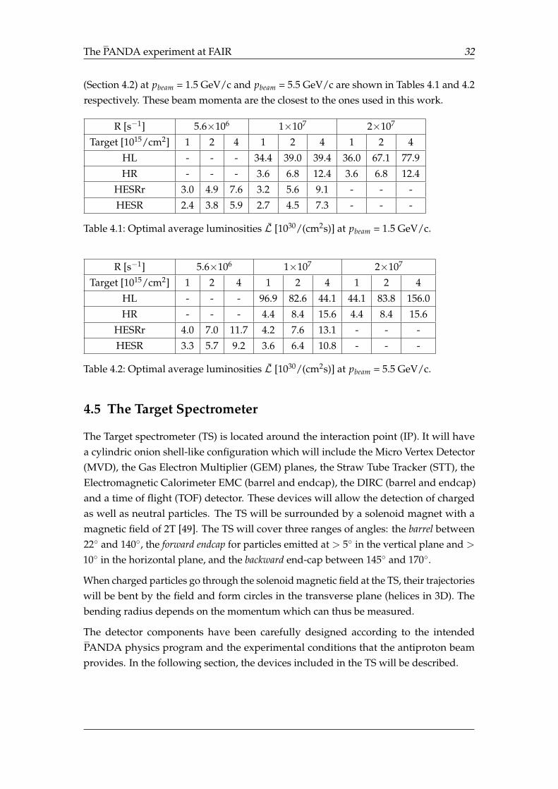
The PANDA experiment at FAIR 32
(Section 4.2) at pbeam = 1.5 GeV/c and pbeam = 5.5 GeV/c are shown in Tables 4.1 and 4.2respectively. These beam momenta are the closest to the ones used in this work.
R [s−1] 5.6×10⁶ 1×10⁷ 2×10⁷
Target [1015/cm2] 1 2 4 1 2 4 1 2 4
HL - - - 34.4 39.0 39.4 36.0 67.1 77.9
HR - - - 3.6 6.8 12.4 3.6 6.8 12.4
HESRr 3.0 4.9 7.6 3.2 5.6 9.1 - - -
HESR 2.4 3.8 5.9 2.7 4.5 7.3 - - -
Table 4.1: Optimal average luminosities L [1030/(cm2s)] at pbeam = 1.5 GeV/c.
R [s−1] 5.6×10⁶ 1×10⁷ 2×10⁷
Target [1015/cm2] 1 2 4 1 2 4 1 2 4
HL - - - 96.9 82.6 44.1 44.1 83.8 156.0
HR - - - 4.4 8.4 15.6 4.4 8.4 15.6
HESRr 4.0 7.0 11.7 4.2 7.6 13.1 - - -
HESR 3.3 5.7 9.2 3.6 6.4 10.8 - - -
Table 4.2: Optimal average luminosities L [1030/(cm2s)] at pbeam = 5.5 GeV/c.
4.5 The Target Spectrometer
The Target spectrometer (TS) is located around the interaction point (IP). It will havea cylindric onion shell-like configuration which will include the Micro Vertex Detector(MVD), the Gas Electron Multiplier (GEM) planes, the Straw Tube Tracker (STT), theElectromagnetic Calorimeter EMC (barrel and endcap), the DIRC (barrel and endcap)and a time of flight (TOF) detector. These devices will allow the detection of chargedas well as neutral particles. The TS will be surrounded by a solenoid magnet with amagnetic field of 2T [49]. The TS will cover three ranges of angles: the barrel between22 and 140, the forward endcap for particles emitted at > 5 in the vertical plane and >
10 in the horizontal plane, and the backward end-cap between 145 and 170.
When charged particles go through the solenoid magnetic field at the TS, their trajectorieswill be bent by the field and form circles in the transverse plane (helices in 3D). Thebending radius depends on the momentum which can thus be measured.
The detector components have been carefully designed according to the intendedPANDA physics program and the experimental conditions that the antiproton beamprovides. In the following section, the devices included in the TS will be described.
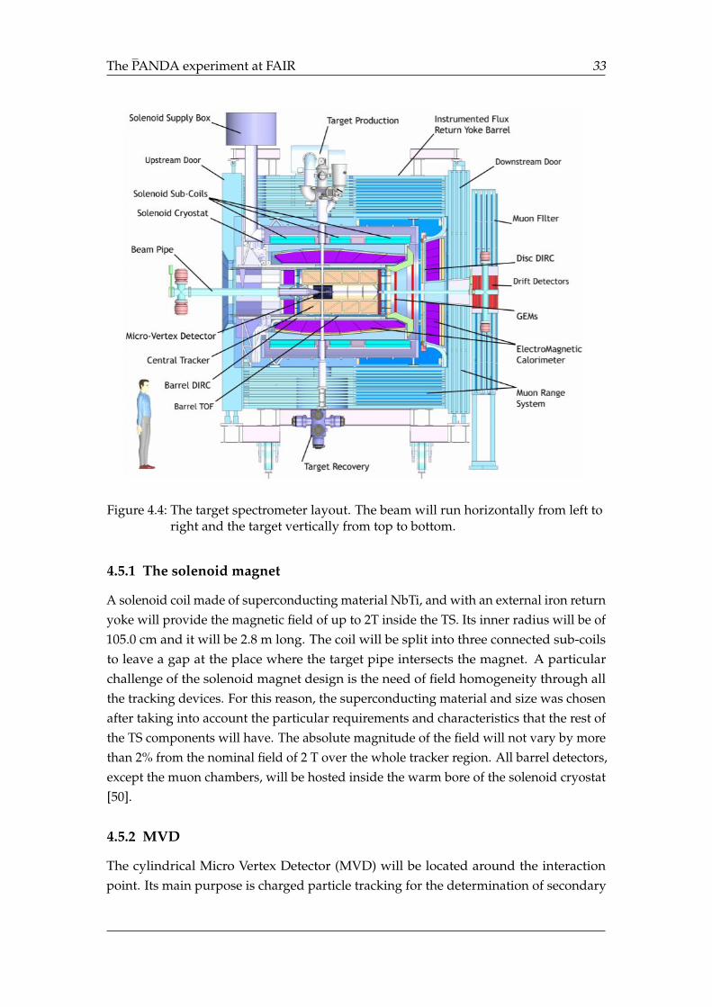
The PANDA experiment at FAIR 33
Figure 4.4: The target spectrometer layout. The beam will run horizontally from left toright and the target vertically from top to bottom.
4.5.1 The solenoid magnet
A solenoid coil made of superconducting material NbTi, and with an external iron returnyoke will provide the magnetic field of up to 2T inside the TS. Its inner radius will be of105.0 cm and it will be 2.8 m long. The coil will be split into three connected sub-coilsto leave a gap at the place where the target pipe intersects the magnet. A particularchallenge of the solenoid magnet design is the need of field homogeneity through allthe tracking devices. For this reason, the superconducting material and size was chosenafter taking into account the particular requirements and characteristics that the rest ofthe TS components will have. The absolute magnitude of the field will not vary by morethan 2% from the nominal field of 2 T over the whole tracker region. All barrel detectors,except the muon chambers, will be hosted inside the warm bore of the solenoid cryostat[50].
4.5.2 MVD
The cylindrical Micro Vertex Detector (MVD) will be located around the interactionpoint. Its main purpose is charged particle tracking for the determination of secondary
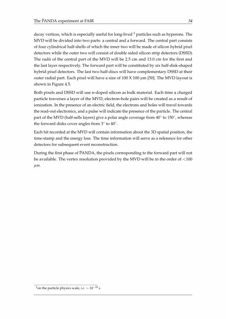
The PANDA experiment at FAIR 34
decay vertices, which is especially useful for long-lived 2 particles such as hyperons. TheMVD will be divided into two parts: a central and a forward. The central part consistsof four cylindrical half-shells of which the inner two will be made of silicon hybrid pixeldetectors while the outer two will consist of double sided silicon strip detectors (DSSD).The radii of the central part of the MVD will be 2.5 cm and 13.0 cm for the first andthe last layer respectively. The forward part will be constituted by six half-disk-shapedhybrid pixel detectors. The last two half-discs will have complementary DSSD at theirouter radial part. Each pixel will have a size of 100 X 100 µm [50]. The MVD layout isshown in Figure 4.5.
Both pixels and DSSD will use n-doped silicon as bulk material. Each time a chargedparticle traverses a layer of the MVD, electron-hole pairs will be created as a result ofionization. In the presence of an electric field, the electrons and holes will travel towardsthe read-out electronics, and a pulse will indicate the presence of the particle. The centralpart of the MVD (half-sells layers) give a polar angle coverage from 40 to 150, whereasthe forward disks cover angles from 3 to 40.
Each hit recorded at the MVD will contain information about the 3D spatial position, thetime-stamp and the energy loss. The time information will serve as a reference for otherdetectors for subsequent event reconstruction.
During the first phase of PANDA, the pixels corresponding to the forward part will notbe available. The vertex resolution provided by the MVD will be in the order of <100µm.
2on the particle physics scale, i.e. ∼ 10−10 s
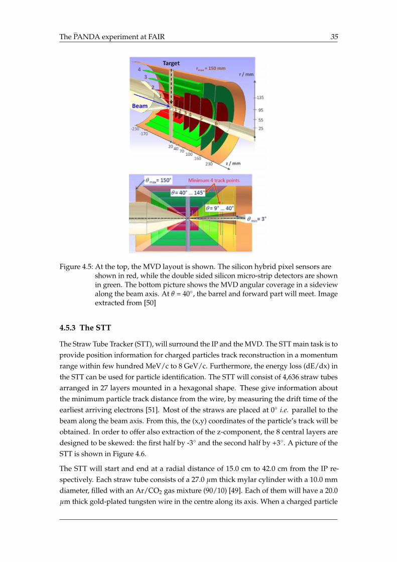
The PANDA experiment at FAIR 35
Figure 4.5: At the top, the MVD layout is shown. The silicon hybrid pixel sensors areshown in red, while the double sided silicon micro-strip detectors are shownin green. The bottom picture shows the MVD angular coverage in a sideviewalong the beam axis. At θ = 40, the barrel and forward part will meet. Imageextracted from [50]
4.5.3 The STT
The Straw Tube Tracker (STT), will surround the IP and the MVD. The STT main task is toprovide position information for charged particles track reconstruction in a momentumrange within few hundred MeV/c to 8 GeV/c. Furthermore, the energy loss (dE/dx) inthe STT can be used for particle identification. The STT will consist of 4,636 straw tubesarranged in 27 layers mounted in a hexagonal shape. These give information aboutthe minimum particle track distance from the wire, by measuring the drift time of theearliest arriving electrons [51]. Most of the straws are placed at 0 i.e. parallel to thebeam along the beam axis. From this, the (x,y) coordinates of the particle’s track will beobtained. In order to offer also extraction of the z-component, the 8 central layers aredesigned to be skewed: the first half by -3 and the second half by +3. A picture of theSTT is shown in Figure 4.6.
The STT will start and end at a radial distance of 15.0 cm to 42.0 cm from the IP re-spectively. Each straw tube consists of a 27.0 µm thick mylar cylinder with a 10.0 mmdiameter, filled with an Ar/CO2 gas mixture (90/10) [49]. Each of them will have a 20.0µm thick gold-plated tungsten wire in the centre along its axis. When a charged particle
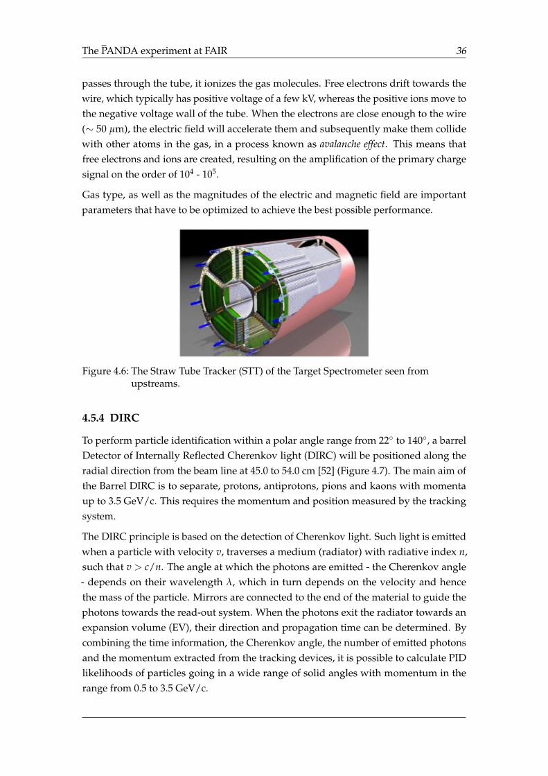
The PANDA experiment at FAIR 36
passes through the tube, it ionizes the gas molecules. Free electrons drift towards thewire, which typically has positive voltage of a few kV, whereas the positive ions move tothe negative voltage wall of the tube. When the electrons are close enough to the wire(∼ 50 µm), the electric field will accelerate them and subsequently make them collidewith other atoms in the gas, in a process known as avalanche effect. This means thatfree electrons and ions are created, resulting on the amplification of the primary chargesignal on the order of 104 - 105.
Gas type, as well as the magnitudes of the electric and magnetic field are importantparameters that have to be optimized to achieve the best possible performance.
Figure 4.6: The Straw Tube Tracker (STT) of the Target Spectrometer seen fromupstreams.
4.5.4 DIRC
To perform particle identification within a polar angle range from 22 to 140, a barrelDetector of Internally Reflected Cherenkov light (DIRC) will be positioned along theradial direction from the beam line at 45.0 to 54.0 cm [52] (Figure 4.7). The main aim ofthe Barrel DIRC is to separate, protons, antiprotons, pions and kaons with momentaup to 3.5 GeV/c. This requires the momentum and position measured by the trackingsystem.
The DIRC principle is based on the detection of Cherenkov light. Such light is emittedwhen a particle with velocity v, traverses a medium (radiator) with radiative index n,such that v > c/n. The angle at which the photons are emitted - the Cherenkov angle- depends on their wavelength λ, which in turn depends on the velocity and hencethe mass of the particle. Mirrors are connected to the end of the material to guide thephotons towards the read-out system. When the photons exit the radiator towards anexpansion volume (EV), their direction and propagation time can be determined. Bycombining the time information, the Cherenkov angle, the number of emitted photonsand the momentum extracted from the tracking devices, it is possible to calculate PIDlikelihoods of particles going in a wide range of solid angles with momentum in therange from 0.5 to 3.5 GeV/c.
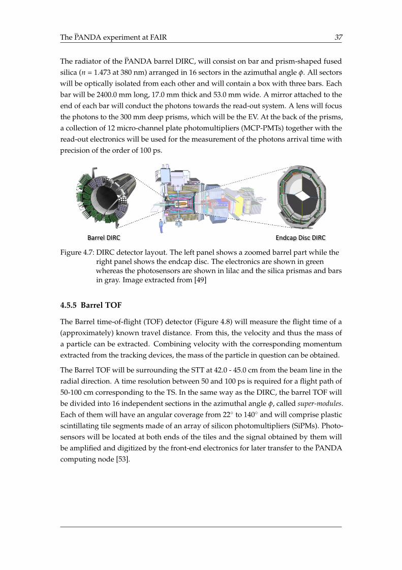
The PANDA experiment at FAIR 37
The radiator of the PANDA barrel DIRC, will consist on bar and prism-shaped fusedsilica (n = 1.473 at 380 nm) arranged in 16 sectors in the azimuthal angle φ. All sectorswill be optically isolated from each other and will contain a box with three bars. Eachbar will be 2400.0 mm long, 17.0 mm thick and 53.0 mm wide. A mirror attached to theend of each bar will conduct the photons towards the read-out system. A lens will focusthe photons to the 300 mm deep prisms, which will be the EV. At the back of the prisms,a collection of 12 micro-channel plate photomultipliers (MCP-PMTs) together with theread-out electronics will be used for the measurement of the photons arrival time withprecision of the order of 100 ps.
Figure 4.7: DIRC detector layout. The left panel shows a zoomed barrel part while theright panel shows the endcap disc. The electronics are shown in greenwhereas the photosensors are shown in lilac and the silica prismas and barsin gray. Image extracted from [49]
4.5.5 Barrel TOF
The Barrel time-of-flight (TOF) detector (Figure 4.8) will measure the flight time of a(approximately) known travel distance. From this, the velocity and thus the mass ofa particle can be extracted. Combining velocity with the corresponding momentumextracted from the tracking devices, the mass of the particle in question can be obtained.
The Barrel TOF will be surrounding the STT at 42.0 - 45.0 cm from the beam line in theradial direction. A time resolution between 50 and 100 ps is required for a flight path of50-100 cm corresponding to the TS. In the same way as the DIRC, the barrel TOF willbe divided into 16 independent sections in the azimuthal angle φ, called super-modules.Each of them will have an angular coverage from 22 to 140 and will comprise plasticscintillating tile segments made of an array of silicon photomultipliers (SiPMs). Photo-sensors will be located at both ends of the tiles and the signal obtained by them willbe amplified and digitized by the front-end electronics for later transfer to the PANDAcomputing node [53].
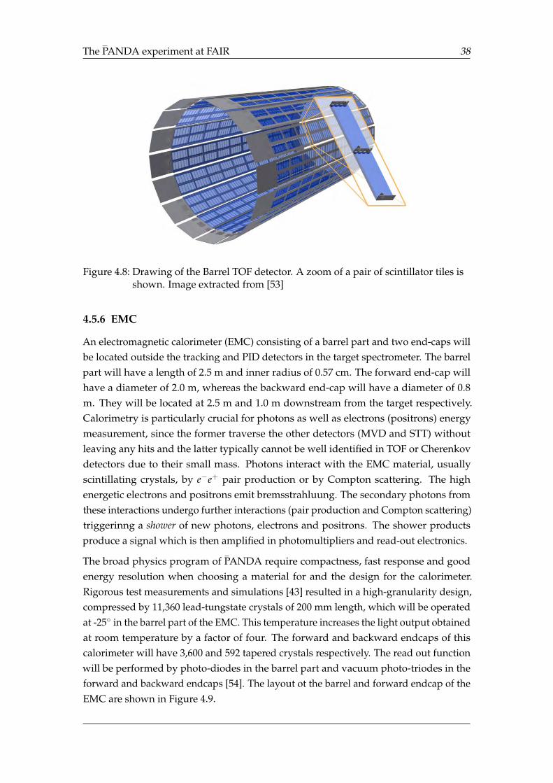
The PANDA experiment at FAIR 38
Figure 4.8: Drawing of the Barrel TOF detector. A zoom of a pair of scintillator tiles isshown. Image extracted from [53]
4.5.6 EMC
An electromagnetic calorimeter (EMC) consisting of a barrel part and two end-caps willbe located outside the tracking and PID detectors in the target spectrometer. The barrelpart will have a length of 2.5 m and inner radius of 0.57 cm. The forward end-cap willhave a diameter of 2.0 m, whereas the backward end-cap will have a diameter of 0.8m. They will be located at 2.5 m and 1.0 m downstream from the target respectively.Calorimetry is particularly crucial for photons as well as electrons (positrons) energymeasurement, since the former traverse the other detectors (MVD and STT) withoutleaving any hits and the latter typically cannot be well identified in TOF or Cherenkovdetectors due to their small mass. Photons interact with the EMC material, usuallyscintillating crystals, by e−e+ pair production or by Compton scattering. The highenergetic electrons and positrons emit bremsstrahluung. The secondary photons fromthese interactions undergo further interactions (pair production and Compton scattering)triggerinng a shower of new photons, electrons and positrons. The shower productsproduce a signal which is then amplified in photomultipliers and read-out electronics.
The broad physics program of PANDA require compactness, fast response and goodenergy resolution when choosing a material for and the design for the calorimeter.Rigorous test measurements and simulations [43] resulted in a high-granularity design,compressed by 11,360 lead-tungstate crystals of 200 mm length, which will be operatedat -25 in the barrel part of the EMC. This temperature increases the light output obtainedat room temperature by a factor of four. The forward and backward endcaps of thiscalorimeter will have 3,600 and 592 tapered crystals respectively. The read out functionwill be performed by photo-diodes in the barrel part and vacuum photo-triodes in theforward and backward endcaps [54]. The layout ot the barrel and forward endcap of theEMC are shown in Figure 4.9.
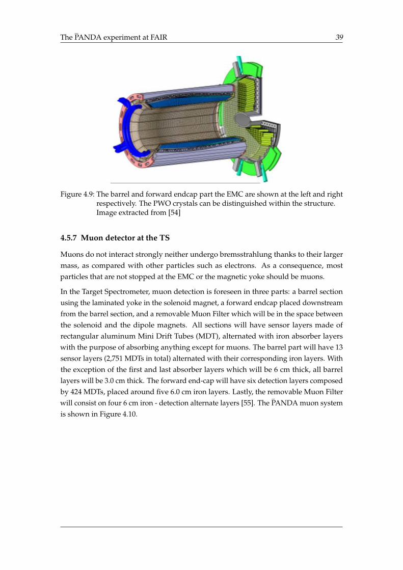
The PANDA experiment at FAIR 39
Figure 4.9: The barrel and forward endcap part the EMC are shown at the left and rightrespectively. The PWO crystals can be distinguished within the structure.Image extracted from [54]
4.5.7 Muon detector at the TS
Muons do not interact strongly neither undergo bremsstrahlung thanks to their largermass, as compared with other particles such as electrons. As a consequence, mostparticles that are not stopped at the EMC or the magnetic yoke should be muons.
In the Target Spectrometer, muon detection is foreseen in three parts: a barrel sectionusing the laminated yoke in the solenoid magnet, a forward endcap placed downstreamfrom the barrel section, and a removable Muon Filter which will be in the space betweenthe solenoid and the dipole magnets. All sections will have sensor layers made ofrectangular aluminum Mini Drift Tubes (MDT), alternated with iron absorber layerswith the purpose of absorbing anything except for muons. The barrel part will have 13sensor layers (2,751 MDTs in total) alternated with their corresponding iron layers. Withthe exception of the first and last absorber layers which will be 6 cm thick, all barrellayers will be 3.0 cm thick. The forward end-cap will have six detection layers composedby 424 MDTs, placed around five 6.0 cm iron layers. Lastly, the removable Muon Filterwill consist on four 6 cm iron - detection alternate layers [55]. The PANDA muon systemis shown in Figure 4.10.
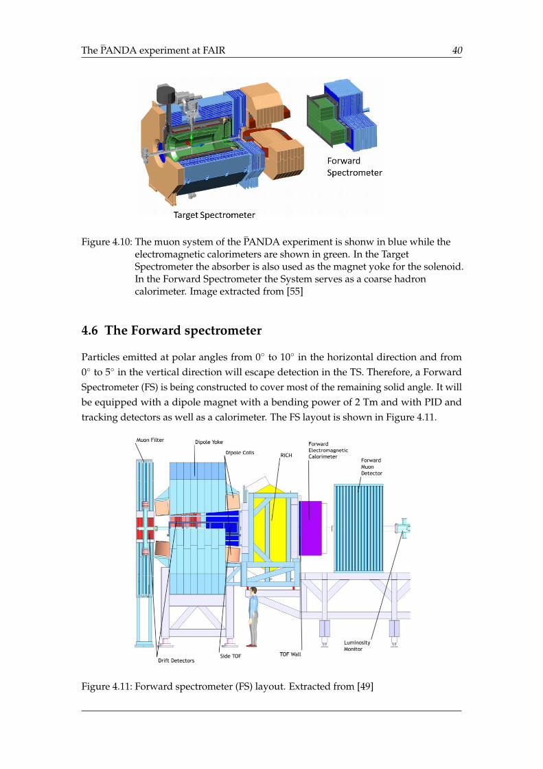
The PANDA experiment at FAIR 40
Figure 4.10: The muon system of the PANDA experiment is shonw in blue while theelectromagnetic calorimeters are shown in green. In the TargetSpectrometer the absorber is also used as the magnet yoke for the solenoid.In the Forward Spectrometer the System serves as a coarse hadroncalorimeter. Image extracted from [55]
4.6 The Forward spectrometer
Particles emitted at polar angles from 0 to 10 in the horizontal direction and from0 to 5 in the vertical direction will escape detection in the TS. Therefore, a ForwardSpectrometer (FS) is being constructed to cover most of the remaining solid angle. It willbe equipped with a dipole magnet with a bending power of 2 Tm and with PID andtracking detectors as well as a calorimeter. The FS layout is shown in Figure 4.11.
Figure 4.11: Forward spectrometer (FS) layout. Extracted from [49]
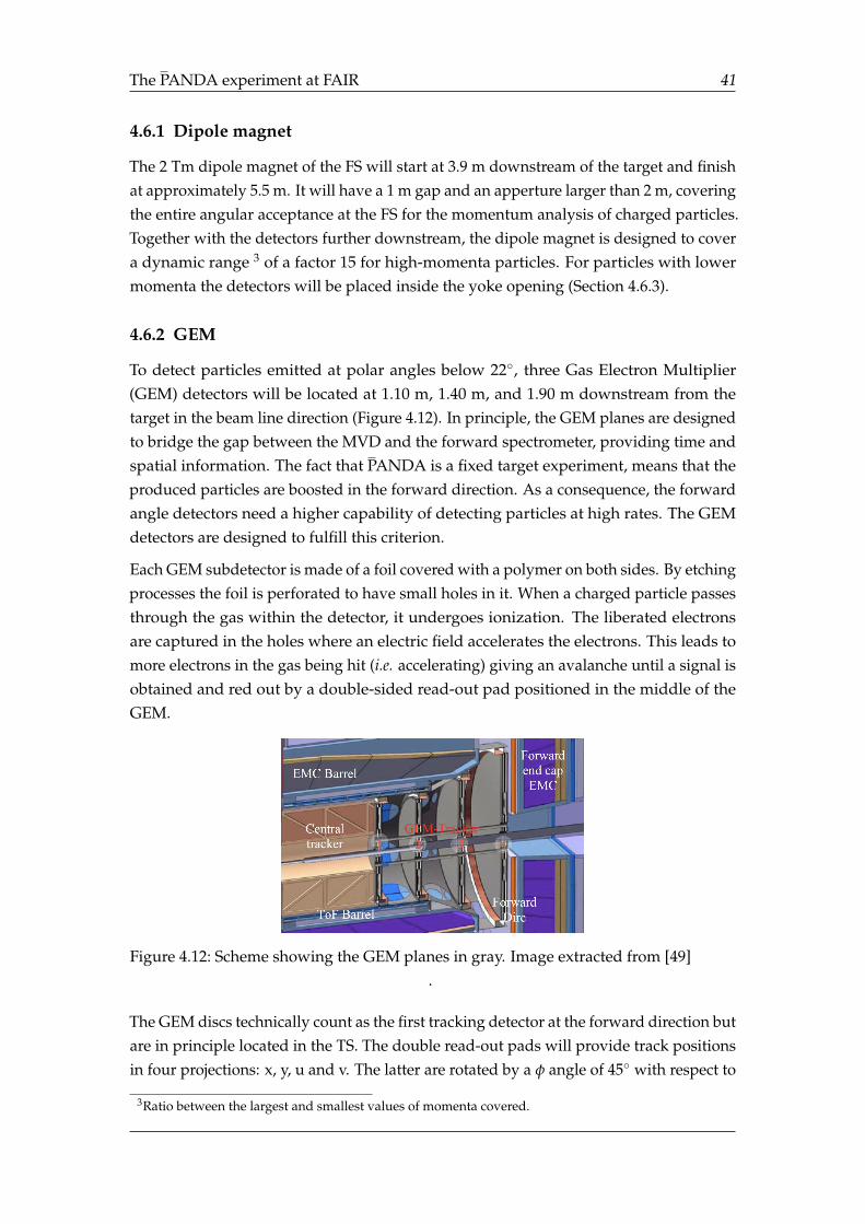
The PANDA experiment at FAIR 41
4.6.1 Dipole magnet
The 2 Tm dipole magnet of the FS will start at 3.9 m downstream of the target and finishat approximately 5.5 m. It will have a 1 m gap and an apperture larger than 2 m, coveringthe entire angular acceptance at the FS for the momentum analysis of charged particles.Together with the detectors further downstream, the dipole magnet is designed to covera dynamic range 3 of a factor 15 for high-momenta particles. For particles with lowermomenta the detectors will be placed inside the yoke opening (Section 4.6.3).
4.6.2 GEM
To detect particles emitted at polar angles below 22, three Gas Electron Multiplier(GEM) detectors will be located at 1.10 m, 1.40 m, and 1.90 m downstream from thetarget in the beam line direction (Figure 4.12). In principle, the GEM planes are designedto bridge the gap between the MVD and the forward spectrometer, providing time andspatial information. The fact that PANDA is a fixed target experiment, means that theproduced particles are boosted in the forward direction. As a consequence, the forwardangle detectors need a higher capability of detecting particles at high rates. The GEMdetectors are designed to fulfill this criterion.
Each GEM subdetector is made of a foil covered with a polymer on both sides. By etchingprocesses the foil is perforated to have small holes in it. When a charged particle passesthrough the gas within the detector, it undergoes ionization. The liberated electronsare captured in the holes where an electric field accelerates the electrons. This leads tomore electrons in the gas being hit (i.e. accelerating) giving an avalanche until a signal isobtained and red out by a double-sided read-out pad positioned in the middle of theGEM.
Figure 4.12: Scheme showing the GEM planes in gray. Image extracted from [49].
The GEM discs technically count as the first tracking detector at the forward direction butare in principle located in the TS. The double read-out pads will provide track positionsin four projections: x, y, u and v. The latter are rotated by a φ angle of 45 with respect to
3Ratio between the largest and smallest values of momenta covered.
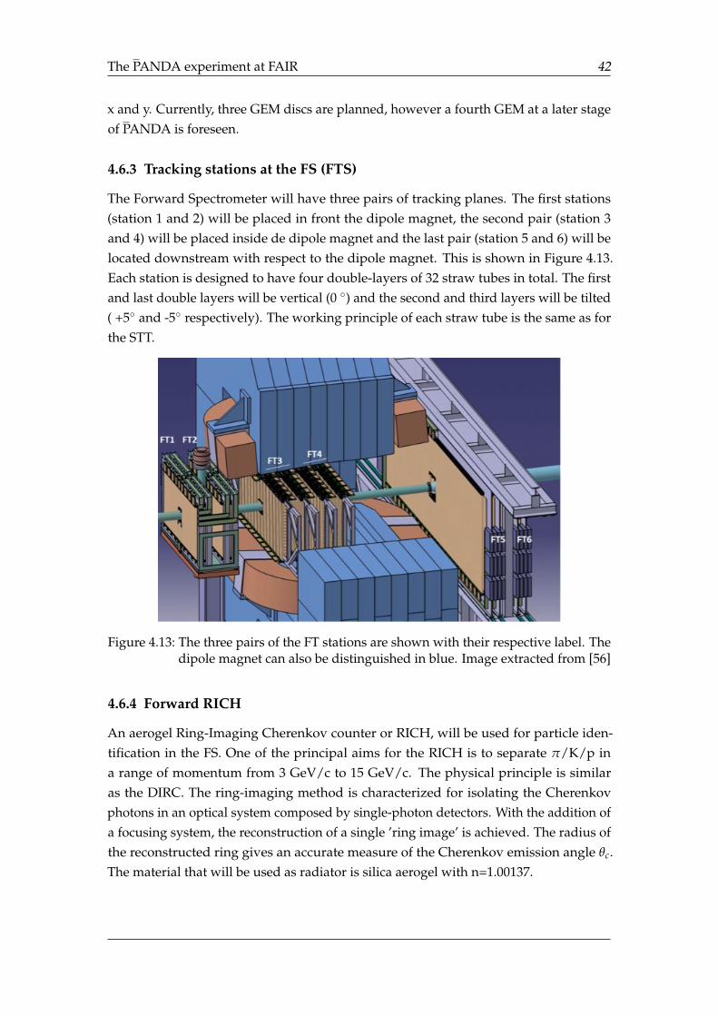
The PANDA experiment at FAIR 42
x and y. Currently, three GEM discs are planned, however a fourth GEM at a later stageof PANDA is foreseen.
4.6.3 Tracking stations at the FS (FTS)
The Forward Spectrometer will have three pairs of tracking planes. The first stations(station 1 and 2) will be placed in front the dipole magnet, the second pair (station 3and 4) will be placed inside de dipole magnet and the last pair (station 5 and 6) will belocated downstream with respect to the dipole magnet. This is shown in Figure 4.13.Each station is designed to have four double-layers of 32 straw tubes in total. The firstand last double layers will be vertical (0 ) and the second and third layers will be tilted( +5 and -5 respectively). The working principle of each straw tube is the same as forthe STT.
Figure 4.13: The three pairs of the FT stations are shown with their respective label. Thedipole magnet can also be distinguished in blue. Image extracted from [56]
4.6.4 Forward RICH
An aerogel Ring-Imaging Cherenkov counter or RICH, will be used for particle iden-tification in the FS. One of the principal aims for the RICH is to separate π/K/p ina range of momentum from 3 GeV/c to 15 GeV/c. The physical principle is similaras the DIRC. The ring-imaging method is characterized for isolating the Cherenkovphotons in an optical system composed by single-photon detectors. With the addition ofa focusing system, the reconstruction of a single ’ring image’ is achieved. The radius ofthe reconstructed ring gives an accurate measure of the Cherenkov emission angle θc.The material that will be used as radiator is silica aerogel with n=1.00137.
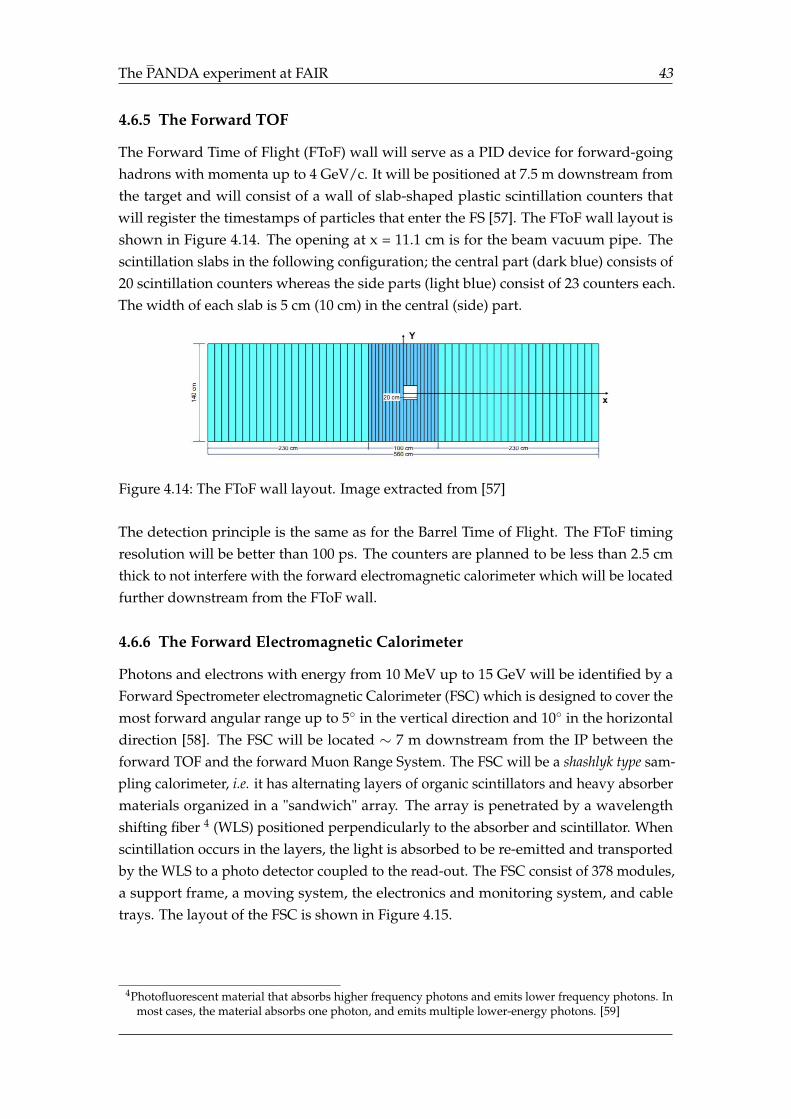
The PANDA experiment at FAIR 43
4.6.5 The Forward TOF
The Forward Time of Flight (FToF) wall will serve as a PID device for forward-goinghadrons with momenta up to 4 GeV/c. It will be positioned at 7.5 m downstream fromthe target and will consist of a wall of slab-shaped plastic scintillation counters thatwill register the timestamps of particles that enter the FS [57]. The FToF wall layout isshown in Figure 4.14. The opening at x = 11.1 cm is for the beam vacuum pipe. Thescintillation slabs in the following configuration; the central part (dark blue) consists of20 scintillation counters whereas the side parts (light blue) consist of 23 counters each.The width of each slab is 5 cm (10 cm) in the central (side) part.
Figure 4.14: The FToF wall layout. Image extracted from [57]
The detection principle is the same as for the Barrel Time of Flight. The FToF timingresolution will be better than 100 ps. The counters are planned to be less than 2.5 cmthick to not interfere with the forward electromagnetic calorimeter which will be locatedfurther downstream from the FToF wall.
4.6.6 The Forward Electromagnetic Calorimeter
Photons and electrons with energy from 10 MeV up to 15 GeV will be identified by aForward Spectrometer electromagnetic Calorimeter (FSC) which is designed to cover themost forward angular range up to 5 in the vertical direction and 10 in the horizontaldirection [58]. The FSC will be located ∼ 7 m downstream from the IP between theforward TOF and the forward Muon Range System. The FSC will be a shashlyk type sam-pling calorimeter, i.e. it has alternating layers of organic scintillators and heavy absorbermaterials organized in a "sandwich" array. The array is penetrated by a wavelengthshifting fiber 4 (WLS) positioned perpendicularly to the absorber and scintillator. Whenscintillation occurs in the layers, the light is absorbed to be re-emitted and transportedby the WLS to a photo detector coupled to the read-out. The FSC consist of 378 modules,a support frame, a moving system, the electronics and monitoring system, and cabletrays. The layout of the FSC is shown in Figure 4.15.
4Photofluorescent material that absorbs higher frequency photons and emits lower frequency photons. Inmost cases, the material absorbs one photon, and emits multiple lower-energy photons. [59]
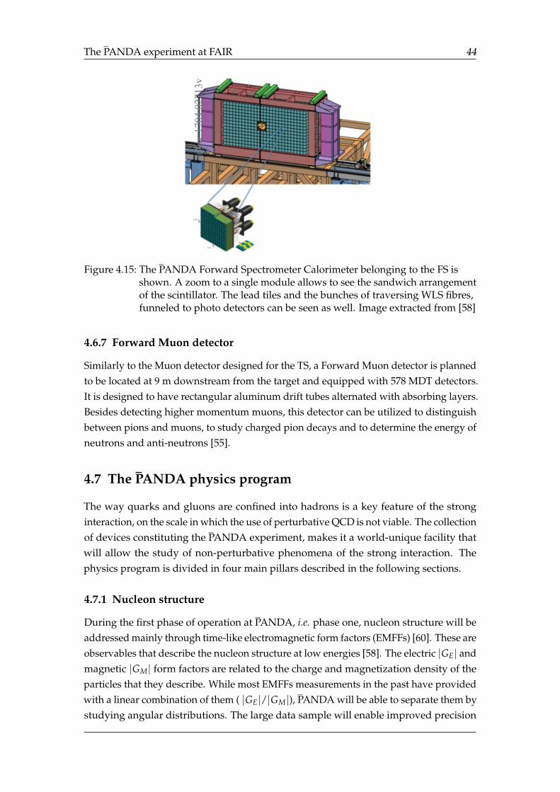
The PANDA experiment at FAIR 44
Figure 4.15: The PANDA Forward Spectrometer Calorimeter belonging to the FS isshown. A zoom to a single module allows to see the sandwich arrangementof the scintillator. The lead tiles and the bunches of traversing WLS fibres,funneled to photo detectors can be seen as well. Image extracted from [58]
4.6.7 Forward Muon detector
Similarly to the Muon detector designed for the TS, a Forward Muon detector is plannedto be located at 9 m downstream from the target and equipped with 578 MDT detectors.It is designed to have rectangular aluminum drift tubes alternated with absorbing layers.Besides detecting higher momentum muons, this detector can be utilized to distinguishbetween pions and muons, to study charged pion decays and to determine the energy ofneutrons and anti-neutrons [55].
4.7 The PANDA physics program
The way quarks and gluons are confined into hadrons is a key feature of the stronginteraction, on the scale in which the use of perturbative QCD is not viable. The collectionof devices constituting the PANDA experiment, makes it a world-unique facility thatwill allow the study of non-perturbative phenomena of the strong interaction. Thephysics program is divided in four main pillars described in the following sections.
4.7.1 Nucleon structure
During the first phase of operation at PANDA, i.e. phase one, nucleon structure will beaddressed mainly through time-like electromagnetic form factors (EMFFs) [60]. These areobservables that describe the nucleon structure at low energies [58]. The electric |GE| andmagnetic |GM| form factors are related to the charge and magnetization density of theparticles that they describe. While most EMFFs measurements in the past have providedwith a linear combination of them ( |GE|/|GM|), PANDA will be able to separate them bystudying angular distributions. The large data sample will enable improved precision
The PANDA experiment at FAIR 45
with respect to other experiments [46], and will reach higher energies. In addition,PANDA will be able to measure form factors with muons in the final state for the firsttime.
In the later phases of PANDA, the focus is on hard scattering observables. In the time-like region, the structure is described by generalized distribution amplitudes (GDAs)[61] and transition distribution amplitudes (TDAs) [62], [63]. These will be accessedexperimentally through different electromagnetic processes at PANDA.
4.7.2 Strangeness physics
Processes involving strangeness have proven to be a fruitful way to study several sub-atomic physics fundamental questions. One example is the quark model that emergedfrom the observed SU(3) flavor symmetry of the light hadron spectrum (Section 1.4).Properties such as mass, spin, radius and structure of baryons are difficult to understandfrom first principles since they are non-perturbative QCD phenomena. Hyperon produc-tion and spectroscopy are part of the PANDA physics program. In addition, CP violationand its important role in baryogenesis will be addressed through hyperon decay studies.By experiments with secondary target, nuclei containing strange particles, i.e. will bestudied.
Hyperon production
Strange hyperon production sheds light on the strong interaction at low energies (<few GeV). As mentioned at Section 3.1, this is because the production mechanism isgoverned by the strange quark mass ms ∼ 100 MeV, which corresponds to the poorlyunderstood confinement domain.
Spin observables such as polarization and spin correlation, provide important informa-tion about strangeness production and the role of the spin in the structure and interactiondynamics. Spontaneous chiral symmetry breaking, the hadrons and quarks masses, aswell as quark confinement, are some of the non-perturbative phenomena that can beconnected to spin effects. Hyperon polarization can be determined by measuring theangular distributions of its decay products. This will be achieved by taking advantageof the identification of both charged and neutral particles in the 4π coverage detectionthat PANDA will offer.
Hyperon spectroscopy
There are several open questions about the light and strange baryon spectrum. Forinstance, there are many states predicted by the quark model which have not beenexperimentally observed. With baryon spectroscopy, information about the extent towhich the spectra of baryons follow the systematics of SU(3) flavour symmetry, and theexistence of exotic baryon states, can be obtained.
The PANDA experiment at FAIR 46
The high production rate of baryon-antibaryon pairs in PANDA opens up the possibilityof studying the spectrum of baryons which contain one or several strange quarks(hyperons) or a single charmed quarks (charmed-hyperons).
Hypernuclear Physics
If one or more of the nucleons in a nucleus is replaced by a hyperon, a hypernucleusis created. A consequence of the replacement is the addition of strangeness as a newdegree of freedom [49]. Hypernuclei studies lead to a better understanding of the nuclearstructure [21] and the interactions between hadrons. This is crucial e.g. when describinthe physics of neutron stars. Thanks to the high cross-section of hyperon production inpp annihilations, an abundant production of hypernuclei is expected in PANDA. Thisalso includes double hypernuclei, which addresses the hyperon-hyperon interaction.
4.7.3 Charm and exotics
The charmonium system is a powerful testing ground for strong interaction models, inthe region just below the point where perturbative QCD breaks down. At this point,the interaction scale is governed by the charm quark (mc ∼ 1.275 MeV) which is morethan ten times heavier than the strange quark. In charm physics, one refers to open charm(e.g. D-mesons) to the states which consist of a charm quark and a lighter quark, andcharmonium i.e. cc.
Charmonium spectroscopy
The so-called XYZ-states: X(3872), X(3940), Y(3940), Z±c (3930) and Y(4260), are the mostrecent charmonia findings [64]. These states are interesting since they do not fit intothe regular qq-squeme. For instance, the Z±c (3930) has a minimum quark content ofqqqq. To gain a complete understanding of these states, measurements of decay channels,branching ratios and angular distributions will be crucial. The almost full solid anglecoverage of PANDA, and its capability to detect and identify both neutral and chargedfinal states, makes it perfect for addressing the XYZ-states yet unknown properties, e.g.their JPC quantum numbers. Precision measurements of masses, widths and partialdecay widths of charmonium states are also envisaged at PANDA.
Search for Exotics
As mentioned in Section 1.4, baryons (qqq) and mesons (qq) are the configurations, thathave most abundantly been predicted and found experimentally. However, QCD allowsother combinations as long as they are colorless. The aforementioned XYZ-states areoften referred to as candidates for tetraquarks (qqqq) and there have been claims bythe LHCb about the finding of a pentaquark (qqqqq). However, gluonic hadrons likeglueballs and hybrids have not yet been unambiguously identified. In glueballs, the
The PANDA experiment at FAIR 47
contribution to the quantum numbers is only attributed to gluons, whereas for hybridsthey are attributed to both valence quarks (anti-quarks) and one or several excitedgluons.
Charmonium states are narrow, well separated and the mixing effects are much smallerthan in the light-quark sector, making the charmonium system very suitable for theexotics search. Hadron-hadron annihilation is classified as a gluon-rich environment,where hybrids and glueballs are likely to be produced if they exist. The pp annihilationis expected to provide hard gluons from the quark-antiquark annihilation. Therefore, atthe PANDA experiment the search of gluonic excitations and exotic states is included[46] .
Light meson spectroscopy
In addition to hadrons containing c quarks, mesons containing u, d and s quarks willbe studied at PANDA. Even though light meson states are well described by the quarkmodel, there are still some unsolved questions, such as the relevant degrees of freedom orthe existence of gluonic and meson-like excitations. Glueballs, hybrids and multiquarkscould occur also at masses within the light hadron spectra, though they are more difficultto identify due to mixing with other non-exotic states. PANDA will be able to producesuch states at an unprecedented rate.
4.7.4 Hadrons in nuclei
The nuclear targets used at PANDA will open the possibility of studying some featuresof the strong interaction that cannot be studied in vacuum. In particular, the hadronicformation time can be studied focusing on a phenomena called color transparency, i.e.the hypothesis that objects with a very small size have a small reaction cross section.Moreover, the nuclear medium could be studied with large momentum transfer inter-actions. In-medium modifications of hadrons embedded in hadronic matter will bestudied to understand the origin of hadron masses [58]. The p beam with momentumof up to 15 GeV/c will allow an extension of this program to the charm sector throughantiproton-nucleus collisions at PANDA [21].
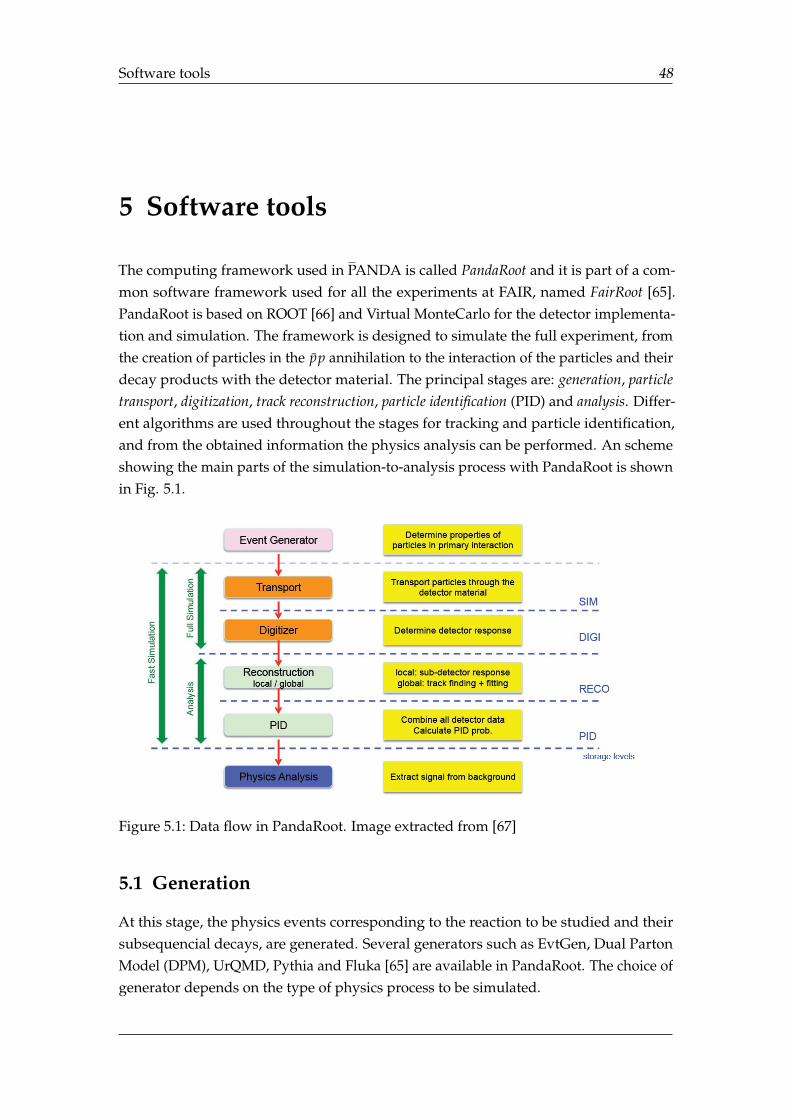
Software tools 48
5 Software tools
The computing framework used in PANDA is called PandaRoot and it is part of a com-mon software framework used for all the experiments at FAIR, named FairRoot [65].PandaRoot is based on ROOT [66] and Virtual MonteCarlo for the detector implementa-tion and simulation. The framework is designed to simulate the full experiment, fromthe creation of particles in the pp annihilation to the interaction of the particles and theirdecay products with the detector material. The principal stages are: generation, particletransport, digitization, track reconstruction, particle identification (PID) and analysis. Differ-ent algorithms are used throughout the stages for tracking and particle identification,and from the obtained information the physics analysis can be performed. An schemeshowing the main parts of the simulation-to-analysis process with PandaRoot is shownin Fig. 5.1.
Figure 5.1: Data flow in PandaRoot. Image extracted from [67]
5.1 Generation
At this stage, the physics events corresponding to the reaction to be studied and theirsubsequencial decays, are generated. Several generators such as EvtGen, Dual PartonModel (DPM), UrQMD, Pythia and Fluka [65] are available in PandaRoot. The choice ofgenerator depends on the type of physics process to be simulated.
Software tools 49
The EvtGen and DPM generators were used in this work. EvtGen is controlled by a decaytable listing all possible decay processes, their branching ratios, and their correspondingdecay model [46]. One of its advantages is that it can handle complex sequential decaychannels taking into account known decay properties, such as angular distributions orpolarization. The decay chain is set by the user, who can also implement decay models.The latter are sometimes based on experimental data.
The reaction pp→ Σ0Λ with the subsequent Σ0 and Λ decay, was modeled by WalterIkegami Andersson1 using a parametrization based on the experimental data describedin section 3.2, where a forward peaked angular distribution was discerned. The EvtGenoutput file consists of a list of all events including information about the generatedparticles and their decay products kinematic properties such as momenta, energy andposition. This file is afterwards used as input for the transport stage [68].
The DPM is a background generator in which all possible hadronic reactions are sim-ulated at a given beam momentum. This generator takes into account differentialcross-sections parametrized from existing experimental data (Section 8.2.1).
5.2 Particle transport
At this stage, the generated particles are propagated through the PANDA sub-detectorsusing GEANT [69], a toolkit for simulating the passage of particles through matter.In GEANT, every detector component and its supporting material is modeled andimplemented. Interactions such as multiple scattering and energy loss by e.g. ionization,[46] as well as effects from traversing magnetic fields are also accounted for. Theusage of Virtual MonteCarlo [70], allows to choose between different transport modelssuch as GEANT3 or GEANT4 [71]. Magnetic fields are described using TOSCA [65]calculations which computes magneto-static and electro-static fields in three dimensions.The information stored from this step corresponds to the energy losses at the intersectionpoints of the particles in the detector components, giving as the output a collection of3D space points called MC-points.
5.3 Digitization
In the MC points, the energy losses are exact and the spatial resolution is infinite. Inreality, the readout electronics provide pulses and the spatial resolution is limited by e.gthe detector granularity. In the digitization step, the detector responses to the particlepassage is modeled, i.e. the obtained output from this stage is in the same form asdetector signals, emulating the data obtained from the experiment. In this way, the samereconstruction software can be used for Monte Carlo data and real data [69].
1PhD student at Uppsala University
Software tools 50
The input from the transport stage into a realistic data stream converts the 3D MC-pointsinto a channel number, and deposited energy into ADC values e.g. pulse heights. Thechannel corresponds to the read-out channel of a detector sensitive component (pixelor tube for instance) which has a given granularity, i.e. finite resolution. Noise andinefficiencies corresponding to real detectors are added as well as electronics properties[67]. After digitization, the new object obtained is called MC-hits.
5.4 Reconstruction
At this stage, hits are clustered into local tracklets within each sub-detector, and subse-quently combined then to form a global track candidate [65]. Tracking information at thetarget spectrometer is provided by the MVD, the STT and the GEM planes. If a centrallygoing charged track leaves either at least four hits in the MVD, or six hits collectivelyin the MVD+STT+GEM, it is considered reconstructible. For forward going particles, atleast six hits in the six straw tubes planes are required for reconstructibility. In addition,the forward GEM planes hits will be used for better resolution.
Reconstruction is performed independently at the TS and the FS in two steps: track findingand track fitting. The former is performed using pattern recognition algorithms. Thereare several algorithms implemented for tracks generated at the interaction point (IP)from the pp collision i.e. primary tracks. However, we are interested in reconstructingtracks belonging to the decay products of Λ and Σ0 hyperons i.e. secondary tracks. Thesedo not originate in the IP and reconstructing them require different pattern recognitionalgorithms, which are still under development in PandaRoot. For this reason, an idealpattern recognition algorithm was used in this work. This method consists on takingall reconstructible tracks adding a standard smearing of σp/p = 0.05 to the true four-momentum components, and σx = 0.05 cm to the position of origin.
For the track fitting, a Kalman filter [72] is used. It does not only take into account themeasurements and their corresponding resolutions, but it also considers the interactionswith detector material such as multiple scattering and energy losses. This is an iterativemethod which requires an initial momentum value and a particle hypothesis as input[73]. In our case the MC-truth momentum with the corresponding smearing is taken asinitial value.
5.5 PID
At this stage, the particles corresponding to each track are identified using the infor-mation from the dedicated PID detectors. In the same way as in the tracking stage, theparticle identification (PID) software is divided into a local and a global part[46]. Locally,each PID sub-detector assigns probabilities for each particle hypothesis (e, µ, π, K andp), calculated according to their corresponding method: energy loss measurements
Software tools 51
(dE/dx) in the STT and MVD, time stamps obtained from the barrel and forward ToFand the Cherenkov angle extracted from the DIRC and RICH detectors. The global PIDis obtained by combining the individual PID information in each sub-detector using amaximum likelihood method.
The global PID value can be optimized using several different algorithms in the analysisstage [74]. These algorithms are defined according to different criteria on the identifi-cation probability value, for example the Loose criterion would require a value P ≥ 0,whereas the Tight criterion would require P ≥ 0.5. In this work, an Ideal PID assignmentwas used, meaning that the MC-truth information is checked in every case in order toassign a probability value of P=1 when the correct particle identity hypothesis is chosenand P = 0 otherwise. This simplifications was necessary since the PID algorithms areunder development.
5.6 Analysis
To perform analysis, a so-called Rho package has been included inside PandaRoot asanalysis tool. Here, the user writes his/her own event selection algorithm and fillcandidate lists. Once the four-momenta of the particles are estimated, variables suchas angles can be calculated from which physical quantities, such as polarisation can beextracted. Access to the MonteCarlo truth information is available for complete studies.In the coming parts of this thesis, my analysis procedure will be described in detail.
Analysis 52
6 Analysis
In a real experiment, a large number of final state particles is produced and detected.One has to distinguish between those that do belong to the reaction of interest, and thosecreated through processes such as cosmic radiation, interaction with passive materialor as a result of other pp annihilations. In general, the analysis strategy followed insimulation studies is to use simulated MonteCarlo (MC) data as a guide to identifyuseful selection criteria that could be applied when real data from the experiment arecollected. In this work, two samples of the reaction pp→ Σ0Λ were simulated:
• The first sample consisting of 10k events generated with a beam momentum ofpbeam = 1.771 GeV/c.
• The second sample consisting of 10k events generated with a beam momentum ofpbeam = 6 GeV/c.
Both simulations were performed using a decay model based on the results obtainedby the different experiments at CERN, explained at section 3.2. The Σ0 baryon decaysalmost at the IP into a Λ (Table 3.1). Thus, the Λ and Λ decay products are the particlesreaching the detectors. As explained in section 5, the first stage of the simulation isthe generation of events. After the generation, five final state particles per event areexpected:
pp→ Σ0Λ→ Λγpπ−→ pπ+γpπ− (6.1)
However, after the generated particles are propagated through the detector material,more particles are created. These can be of the same or different particle species than thefinal state particles. The focus of this analysis is to test the degree at which the Σ0 andΛ corresponding to the simulated channel can be reconstructed and identified. This isachieved by selecting and combining their final state particles measured in the detectors.
The analysis starts by performing an ideal PID match for all the reconstructed particles,i.e. for each charged particle, the correct particle hypothesis is obtained, and it is addedto a list with all the candidates of its particle type. It is important to emphasize that theyare referred to as candidates since even though it is assured that they correspond to theindicated particle type, it is not assured that they originate from the reaction of interest.Four lists of candidates are obtained from this matching (p, p, π+ and π−). On the other
Analysis 53
hand, for neutral particles (γ), the list of candidates is filled using information extractedfrom the calorimeter according to a cut value, explained in more detail at Section 6.3.3.
The kinematics of a reaction gives a general picture about how the momenta or energydistributions of the particles reaching the detectors look like. Based on the comparisonbetween the generated channel vs the reconstructed particles kinematic properties, afirst basic selection is performed as will be explained at section 6.3.2. The selectioncriteria to obtain the Λ, Λ and Σ0 candidates is divided in two stages: pre-selection andfinal selection. The former consist on combining the charged candidates pπ− and pπ+ toreconstruct the Λ and Λ respectively as is further explained at section 6.4. The Σ0 andthe full Σ0Λ channel reconstruction is performed at the latter stage.
Fitting procedures are used at both stages. These are statistical methods which improvethe measurements of certain processes, such as particle interaction or decay, by utilizingknown information e.g. particle masses, energy and momentum conservation. This isreferred to as kinematic fitting [75].
Since the main goal of the analysis is to obtain a sample where false particle candidatesare as few as possible, the final selection (section 6.5) implies tighter kinematic constraintsand more strict criteria for the reconstruction. Two types of event selection methodswere tested: inclusive or and exclusive. The general motivation of these selections isfurther explained in sections 6.1 and 6.2 respectively while the specific details of theprocedures corresponding to this analysis are explained at Chapter 7 for the inclusivecase and at Chapter 8 for the exclusive case.
6.1 Inclusive selection
In the cases where not all final state particles are detected and thus only one part of thesystem can be reconstructed, an inclusive or single tag study is performed. The analysisstrategy in this case consist of extracting the information of the missing particle usingkinematic constraints and conservation laws. Usually a good efficiency is achieved withthis type of selection since less particles have to be reconstructed and thus, the probabilityof not detecting them is lower. On the other hand, fewer kinematic constraints can beimposed, meaning that the background cannot be suppressed to the same extent as ifthe complete system were reconstructed and thus, poorer resolution in e.g momentumand energy is achieved.
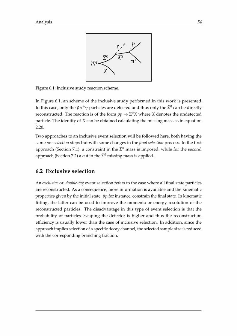
Analysis 54
Figure 6.1: Inclusive study reaction scheme.
In Figure 6.1, an scheme of the inclusive study performed in this work is presented.In this case, only the pπ+γ particles are detected and thus only the Σ0 can be directlyreconstructed. The reaction is of the form pp→ Σ0X where X denotes the undetectedparticle. The identity of X can be obtained calculating the missing mass as in equation2.20.
Two approaches to an inclusive event selection will be followed here, both having thesame pre-selection steps but with some changes in the final selection process. In the firstapproach (Section 7.1), a constraint in the Σ0 mass is imposed, while for the secondapproach (Section 7.2) a cut in the Σ0 missing mass is applied.
6.2 Exclusive selection
An exclusive or double-tag event selection refers to the case where all final state particlesare reconstructed. As a consequence, more information is available and the kinematicproperties given by the initial state, pp for instance, constrain the final state. In kinematicfitting, the latter can be used to improve the momenta or energy resolution of thereconstructed particles. The disadvantage in this type of event selection is that theprobability of particles escaping the detector is higher and thus the reconstructionefficiency is usually lower than the case of inclusive selection. In addition, since theapproach implies selection of a specific decay channel, the selected sample size is reducedwith the corresponding branching fraction.
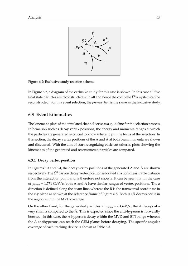
Analysis 55
Figure 6.2: Exclusive study reaction scheme.
In Figure 6.2, a diagram of the exclusive study for this case is shown. In this case all fivefinal state particles are reconstructed with all and hence the complete Σ0Λ system can bereconstructed. For this event selection, the pre-selection is the same as the inclusive study.
6.3 Event kinematics
The kinematic plots of the simulated channel serve as a guideline for the selection process.Information such as decay vertex positions, the energy and momenta ranges at whichthe particles are generated is crucial to know where to put the focus of the selection. Inthis section, the decay vertex positions of the Λ and Λ at both beam momenta are shownand discussed. With the aim of start recognizing basic cut criteria, plots showing thekinematics of the generated and reconstructed particles are compared.
6.3.1 Decay vertex position
In Figures 6.3 and 6.4, the decay vertex positions of the generated Λ and Λ are shownrespectively. The Σ0 baryon decay vertex position is located at a non-measurable distancefrom the interaction point and is therefore not shown. It can be seen that in the caseof pbeam = 1.771 GeV/c, both Λ and Λ have similar ranges of vertex positions. The zdirection is defined along the beam line, whereas the R is the transversal coordinate inthe x-y plane as shown at the reference frame of Figure 6.5. Both Λ/Λ decays occur inthe region within the MVD coverage.
On the other hand, for the generated particles at pbeam = 6 GeV/c, the Λ decays at avery small z compared to the Λ. This is expected since the anti-hyperon is forwardlyboosted. In this case, the Λ hyperons decay within the MVD and STT range whereasthe Λ antihyperons can reach the GEM planes before decaying. The specific angularcoverage of each tracking device is shown at Table 6.3.
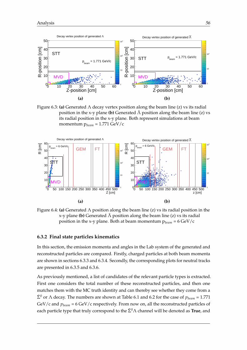
Analysis 56
Z-position [cm]0 10 20 30 40 50 60
R-p
ositi
on [c
m]
0
10
20
30
40
50
1
10
210
310
MVD
STT
GEM
FT
= 1.771 GeV/cbeam
p
ΛDecay vertex position of generated
(a)
Z-position [cm]0 10 20 30 40 50 60
R-p
ositi
on [c
m]
0
10
20
30
40
50
1
10
210
MVD
STT
GEM
FT
= 1.771 GeV/cbeam
p
ΛDecay vertex position of generated
(b)
Figure 6.3: (a) Generated Λ decay vertex position along the beam line (z) vs its radialposition in the x-y plane (b) Generated Λ position along the beam line (z) vsits radial position in the x-y plane. Both represent simulations at beammomentum pbeam = 1.771 GeV/c
Z [cm]0 50 100 150 200 250 300 350 400 450 500
R [c
m]
0
10
20
30
40
50
60
1
10
210
310
MVD
STT
GEM FT = 6 GeV/c
beamp
ΛDecay vertex position of generated
(a)
z [cm]0 50 100 150 200 250 300 350 400 450 500
R [c
m]
0
10
20
30
40
50
60
1
10
210
310
MVD
STT
GEM FT = 6 GeV/c
beamp
ΛDecay vertex position of generated
(b)
Figure 6.4: (a) Generated Λ position along the beam line (z) vs its radial position in thex-y plane (b) Generated Λ position along the beam line (z) vs its radialposition in the x-y plane. Both at beam momentum pbeam = 6 GeV/c
6.3.2 Final state particles kinematics
In this section, the emission momenta and angles in the Lab system of the generated andreconstructed particles are compared. Firstly, charged particles at both beam momentaare shown in sections 6.3.3 and 6.3.4. Secondly, the corresponding plots for neutral tracksare presented in 6.3.5 and 6.3.6.
As previously mentioned, a list of candidates of the relevant particle types is extracted.First one considers the total number of these reconstructed particles, and then onematches them with the MC truth identity and can thereby see whether they come from aΣ0 or Λ decay. The numbers are shown at Table 6.1 and 6.2 for the case of pbeam = 1.771GeV/c and pbeam = 6 GeV/c respectively. From now on, all the reconstructed particles ofeach particle type that truly correspond to the Σ0Λ channel will be denoted as True, and
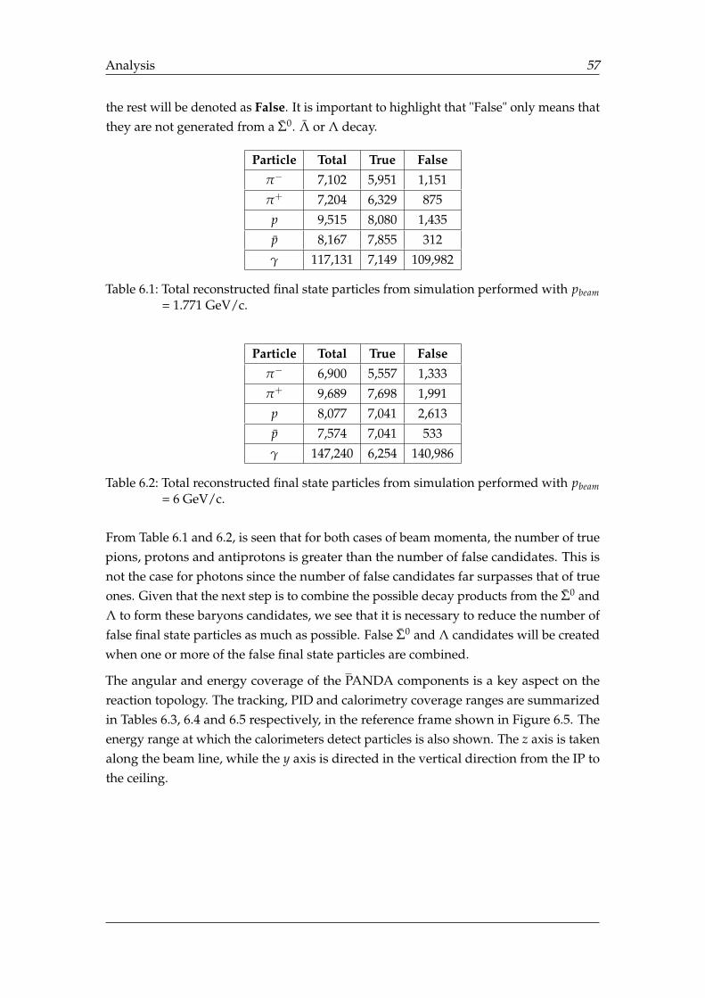
Analysis 57
the rest will be denoted as False. It is important to highlight that "False" only means thatthey are not generated from a Σ0. Λ or Λ decay.
Particle Total True Falseπ− 7,102 5,951 1,151
π+ 7,204 6,329 875
p 9,515 8,080 1,435
p 8,167 7,855 312
γ 117,131 7,149 109,982
Table 6.1: Total reconstructed final state particles from simulation performed with pbeam= 1.771 GeV/c.
Particle Total True Falseπ− 6,900 5,557 1,333
π+ 9,689 7,698 1,991
p 8,077 7,041 2,613
p 7,574 7,041 533
γ 147,240 6,254 140,986
Table 6.2: Total reconstructed final state particles from simulation performed with pbeam= 6 GeV/c.
From Table 6.1 and 6.2, is seen that for both cases of beam momenta, the number of truepions, protons and antiprotons is greater than the number of false candidates. This isnot the case for photons since the number of false candidates far surpasses that of trueones. Given that the next step is to combine the possible decay products from the Σ0 andΛ to form these baryons candidates, we see that it is necessary to reduce the number offalse final state particles as much as possible. False Σ0 and Λ candidates will be createdwhen one or more of the false final state particles are combined.
The angular and energy coverage of the PANDA components is a key aspect on thereaction topology. The tracking, PID and calorimetry coverage ranges are summarizedin Tables 6.3, 6.4 and 6.5 respectively, in the reference frame shown in Figure 6.5. Theenergy range at which the calorimeters detect particles is also shown. The z axis is takenalong the beam line, while the y axis is directed in the vertical direction from the IP tothe ceiling.
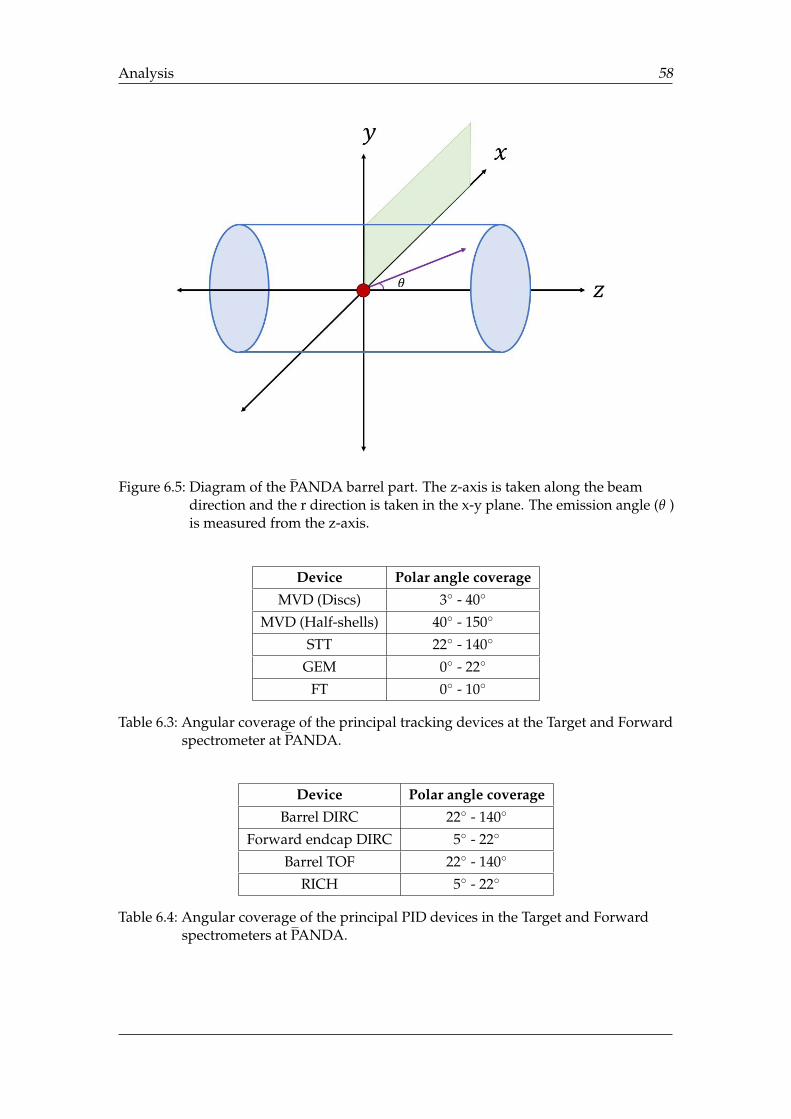
Analysis 58
Figure 6.5: Diagram of the PANDA barrel part. The z-axis is taken along the beamdirection and the r direction is taken in the x-y plane. The emission angle (θ )is measured from the z-axis.
Device Polar angle coverageMVD (Discs) 3 - 40
MVD (Half-shells) 40 - 150
STT 22 - 140
GEM 0 - 22
FT 0 - 10
Table 6.3: Angular coverage of the principal tracking devices at the Target and Forwardspectrometer at PANDA.
Device Polar angle coverageBarrel DIRC 22 - 140
Forward endcap DIRC 5 - 22
Barrel TOF 22 - 140
RICH 5 - 22
Table 6.4: Angular coverage of the principal PID devices in the Target and Forwardspectrometers at PANDA.
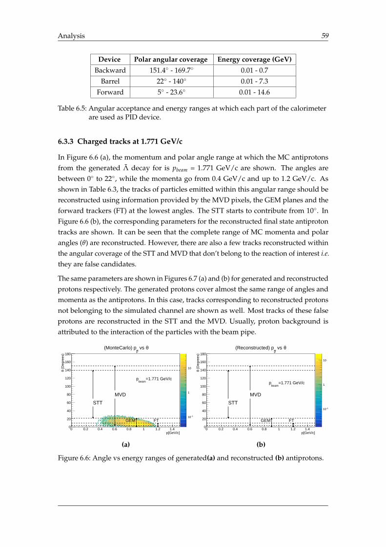
Analysis 59
Device Polar angular coverage Energy coverage (GeV)Backward 151.4 - 169.7 0.01 - 0.7
Barrel 22 - 140 0.01 - 7.3
Forward 5 - 23.6 0.01 - 14.6
Table 6.5: Angular acceptance and energy ranges at which each part of the calorimeterare used as PID device.
6.3.3 Charged tracks at 1.771 GeV/c
In Figure 6.6 (a), the momentum and polar angle range at which the MC antiprotonsfrom the generated Λ decay for is pbeam = 1.771 GeV/c are shown. The angles arebetween 0 to 22, while the momenta go from 0.4 GeV/c and up to 1.2 GeV/c. Asshown in Table 6.3, the tracks of particles emitted within this angular range should bereconstructed using information provided by the MVD pixels, the GEM planes and theforward trackers (FT) at the lowest angles. The STT starts to contribute from 10. InFigure 6.6 (b), the corresponding parameters for the reconstructed final state antiprotontracks are shown. It can be seen that the complete range of MC momenta and polarangles (θ) are reconstructed. However, there are also a few tracks reconstructed withinthe angular coverage of the STT and MVD that don’t belong to the reaction of interest i.e.they are false candidates.
The same parameters are shown in Figures 6.7 (a) and (b) for generated and reconstructedprotons respectively. The generated protons cover almost the same range of angles andmomenta as the antiprotons. In this case, tracks corresponding to reconstructed protonsnot belonging to the simulated channel are shown as well. Most tracks of these falseprotons are reconstructed in the STT and the MVD. Usually, proton background isattributed to the interaction of the particles with the beam pipe.
p[GeV/c]0 0.2 0.4 0.6 0.8 1 1.2 1.4
(D
egre
es)
θ
0
20
40
60
80
100
120
140
160
180
1−10
1
10
MVD
STT
GEM FT
=1.771 GeV/cbeam
p
θ vs p
(MonteCarlo) p
(a)
p[GeV/c]0 0.2 0.4 0.6 0.8 1 1.2 1.4
(D
egre
es)
θ
0
20
40
60
80
100
120
140
160
180
1−10
1
10
MVD
STT
GEM FT
=1.771 GeV/cbeam
p
θ vs p
(Reconstructed) p
(b)
Figure 6.6: Angle vs energy ranges of generated(a) and reconstructed (b) antiprotons.
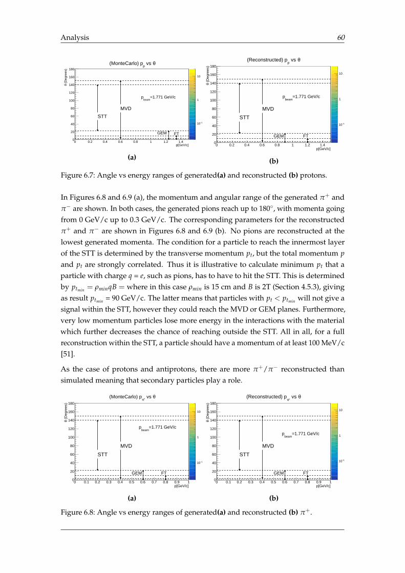
Analysis 60
p[GeV/c]0 0.2 0.4 0.6 0.8 1 1.2 1.4
(D
egre
es)
θ
0
20
40
60
80
100
120
140
160
180
1−10
1
10
MVD
STT
GEM FT
=1.771 GeV/cbeam
p
θ vs p
(MonteCarlo) p
(a)p[GeV/c]
0 0.2 0.4 0.6 0.8 1 1.2 1.4
(D
egre
es)
θ
0
20
40
60
80
100
120
140
160
180
1−10
1
10
MVD
STT
GEM FT
=1.771 GeV/cbeam
p
θ vs p
(Reconstructed) p
(b)
Figure 6.7: Angle vs energy ranges of generated(a) and reconstructed (b) protons.
In Figures 6.8 and 6.9 (a), the momentum and angular range of the generated π+ andπ− are shown. In both cases, the generated pions reach up to 180, with momenta goingfrom 0 GeV/c up to 0.3 GeV/c. The corresponding parameters for the reconstructedπ+ and π− are shown in Figures 6.8 and 6.9 (b). No pions are reconstructed at thelowest generated momenta. The condition for a particle to reach the innermost layerof the STT is determined by the transverse momentum pt, but the total momentum pand pt are strongly correlated. Thus it is illustrative to calculate minimum pt that aparticle with charge q = e, such as pions, has to have to hit the STT. This is determinedby ptmin = ρminqB = where in this case ρmin is 15 cm and B is 2T (Section 4.5.3), givingas result ptmin = 90 GeV/c. The latter means that particles with pt < ptmin will not give asignal within the STT, however they could reach the MVD or GEM planes. Furthermore,very low momentum particles lose more energy in the interactions with the materialwhich further decreases the chance of reaching outside the STT. All in all, for a fullreconstruction within the STT, a particle should have a momentum of at least 100 MeV/c[51].
As the case of protons and antiprotons, there are more π+/π− reconstructed thansimulated meaning that secondary particles play a role.
p[GeV/c]0 0.1 0.2 0.3 0.4 0.5 0.6 0.7 0.8 0.9 1
(D
egre
es)
θ
0
20
40
60
80
100
120
140
160
180
1−10
1
10
MVD
STT
GEM FT
=1.771 GeV/cbeam
p
θ vs +π (MonteCarlo) p
(a)
p[GeV/c]0 0.1 0.2 0.3 0.4 0.5 0.6 0.7 0.8 0.9 1
(D
egre
es)
θ
0
20
40
60
80
100
120
140
160
180
1−10
1
10
MVD
STT
GEM FT
=1.771 GeV/cbeam
p
θ vs +π
(Reconstructed) p
(b)
Figure 6.8: Angle vs energy ranges of generated(a) and reconstructed (b) π+.

Analysis 61
p[GeV/c]0 0.1 0.2 0.3 0.4 0.5 0.6 0.7 0.8 0.9 1
(D
egre
es)
θ
0
20
40
60
80
100
120
140
160
180
1−10
1
10
MVD
STT
GEM FT
=1.771 GeV/cbeam
p
θ vs -π(MonteCarlo) p
(a)
p[GeV/c]0 0.1 0.2 0.3 0.4 0.5 0.6 0.7 0.8 0.9 1
(D
egre
es)
θ
0
20
40
60
80
100
120
140
160
180
1−10
1
10
MVD
STT
GEM FT
=1.771 GeV/cbeam
p
θ vs -π(Reconstructed) p
(b)
Figure 6.9: Angle vs energy ranges of generated(a) and reconstructed (b) π−.
6.3.4 Charged tracks at 6 GeV/c
The momentum range of the generated antiprotons goes from 3 GeV/c up to 5.5 GeV/c(Figure 6.10 (a)). All antiproton tracks are going in the forward direction i.e. they havesmall emission angles. In Figure 6.10 (b), where the same parameters are shown forthe reconstructed antiprotons, most tracks are reconstructed within the FT stations andGEM planes at the correct ranges of momenta and angles. However there are also somefalse antiproton tracks reconstructed in the MVD and STT.
In Figure 6.11 (a) and (b), the corresponding angles and momenta ranges of the generatedand reconstructed protons are shown. Unlike the antiprotons, the protons are notforwardly boosted and have smaller momenta, within 0.2 GeV/c and 2 GeV/c, andangles reaching up to 60. Tracks are reconstructed from hits in all four tracking devices,but the MVD and the STT play a more important role. There are a lot of false protonsemitted at angles up to 180 and with larger momenta (Figure 6.11 (b)).
p[GeV/c]0 1 2 3 4 5 6 7 8
(D
egre
es)
θ
0
20
40
60
80
100
120
140
160
180
1−10
1
10
MVD
STT
GEM FT
= 6 GeV/cbeam
p
θ vs p
(MonteCarlo) p
(a)
p[GeV/c]0 1 2 3 4 5 6 7 8
(D
egre
es)
θ
0
20
40
60
80
100
120
140
160
180
1−10
1
10
MVD
STT
GEM FT
= 6 GeV/cbeam
p
θ vs p
(Reconstructed) p
(b)
Figure 6.10: Angle vs energy ranges of generated(a) and reconstructed (b) antiprotons.
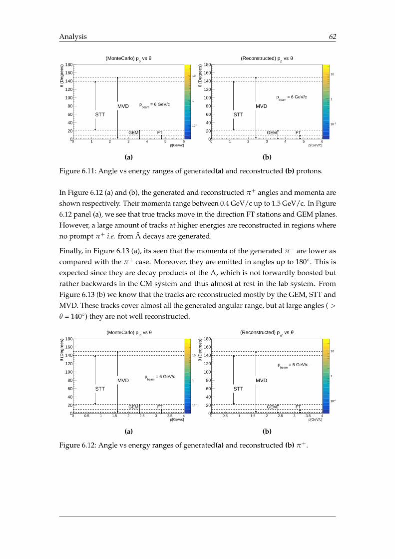
Analysis 62
p[GeV/c]0 1 2 3 4 5 6
(D
egre
es)
θ
0
20
40
60
80
100
120
140
160
180
1−10
1
10
MVD
STT
GEM FT
= 6 GeV/cbeam
p
θ vs p
(MonteCarlo) p
(a)
p[GeV/c]0 1 2 3 4 5 6
(D
egre
es)
θ
0
20
40
60
80
100
120
140
160
180
1−10
1
10
MVD
STT
GEM FT
= 6 GeV/cbeam
p
θ vs p
(Reconstructed) p
(b)
Figure 6.11: Angle vs energy ranges of generated(a) and reconstructed (b) protons.
In Figure 6.12 (a) and (b), the generated and reconstructed π+ angles and momenta areshown respectively. Their momenta range between 0.4 GeV/c up to 1.5 GeV/c. In Figure6.12 panel (a), we see that true tracks move in the direction FT stations and GEM planes.However, a large amount of tracks at higher energies are reconstructed in regions whereno prompt π+ i.e. from Λ decays are generated.
Finally, in Figure 6.13 (a), its seen that the momenta of the generated π− are lower ascompared with the π+ case. Moreover, they are emitted in angles up to 180. This isexpected since they are decay products of the Λ, which is not forwardly boosted butrather backwards in the CM system and thus almost at rest in the lab system. FromFigure 6.13 (b) we know that the tracks are reconstructed mostly by the GEM, STT andMVD. These tracks cover almost all the generated angular range, but at large angles ( >θ = 140) they are not well reconstructed.
p[GeV/c]0 0.5 1 1.5 2 2.5 3 3.5 4
(D
egre
es)
θ
0
20
40
60
80
100
120
140
160
180
1−10
1
10
MVD
STT
GEM FT
= 6 GeV/cbeam
p
θ vs +π (MonteCarlo) p
(a)
p[GeV/c]0 0.5 1 1.5 2 2.5 3 3.5 4
(D
egre
es)
θ
0
20
40
60
80
100
120
140
160
180
1−10
1
10
MVD
STT
GEM FT
= 6 GeV/cbeam
p
θ vs +π
(Reconstructed) p
(b)
Figure 6.12: Angle vs energy ranges of generated(a) and reconstructed (b) π+.
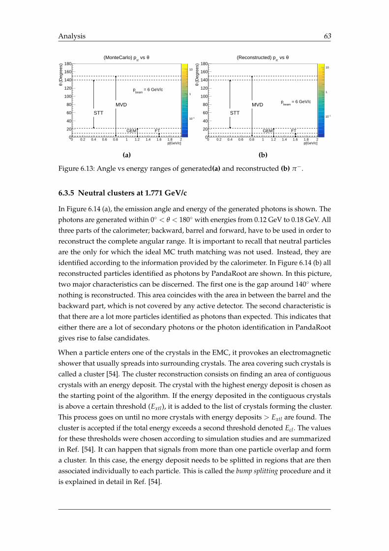
Analysis 63
p[GeV/c]0 0.2 0.4 0.6 0.8 1 1.2 1.4 1.6 1.8 2
(D
egre
es)
θ
0
20
40
60
80
100
120
140
160
180
1−10
1
10
MVD
STT
GEM FT
= 6 GeV/cbeam
p
θ vs -π(MonteCarlo) p
(a)
p[GeV/c]0 0.2 0.4 0.6 0.8 1 1.2 1.4 1.6 1.8 2
(D
egre
es)
θ
0
20
40
60
80
100
120
140
160
180
1−10
1
10
MVD
STT
GEM FT
= 6 GeV/cbeam
p
θ vs -π(Reconstructed) p
(b)
Figure 6.13: Angle vs energy ranges of generated(a) and reconstructed (b) π−.
6.3.5 Neutral clusters at 1.771 GeV/c
In Figure 6.14 (a), the emission angle and energy of the generated photons is shown. Thephotons are generated within 0 < θ < 180 with energies from 0.12 GeV to 0.18 GeV. Allthree parts of the calorimeter; backward, barrel and forward, have to be used in order toreconstruct the complete angular range. It is important to recall that neutral particlesare the only for which the ideal MC truth matching was not used. Instead, they areidentified according to the information provided by the calorimeter. In Figure 6.14 (b) allreconstructed particles identified as photons by PandaRoot are shown. In this picture,two major characteristics can be discerned. The first one is the gap around 140 wherenothing is reconstructed. This area coincides with the area in between the barrel and thebackward part, which is not covered by any active detector. The second characteristic isthat there are a lot more particles identified as photons than expected. This indicates thateither there are a lot of secondary photons or the photon identification in PandaRootgives rise to false candidates.
When a particle enters one of the crystals in the EMC, it provokes an electromagneticshower that usually spreads into surrounding crystals. The area covering such crystals iscalled a cluster [54]. The cluster reconstruction consists on finding an area of contiguouscrystals with an energy deposit. The crystal with the highest energy deposit is chosen asthe starting point of the algorithm. If the energy deposited in the contiguous crystalsis above a certain threshold (Extl), it is added to the list of crystals forming the cluster.This process goes on until no more crystals with energy deposits > Extl are found. Thecluster is accepted if the total energy exceeds a second threshold denoted Ecl . The valuesfor these thresholds were chosen according to simulation studies and are summarizedin Ref. [54]. It can happen that signals from more than one particle overlap and forma cluster. In this case, the energy deposit needs to be splitted in regions that are thenassociated individually to each particle. This is called the bump splitting procedure and itis explained in detail in Ref. [54].
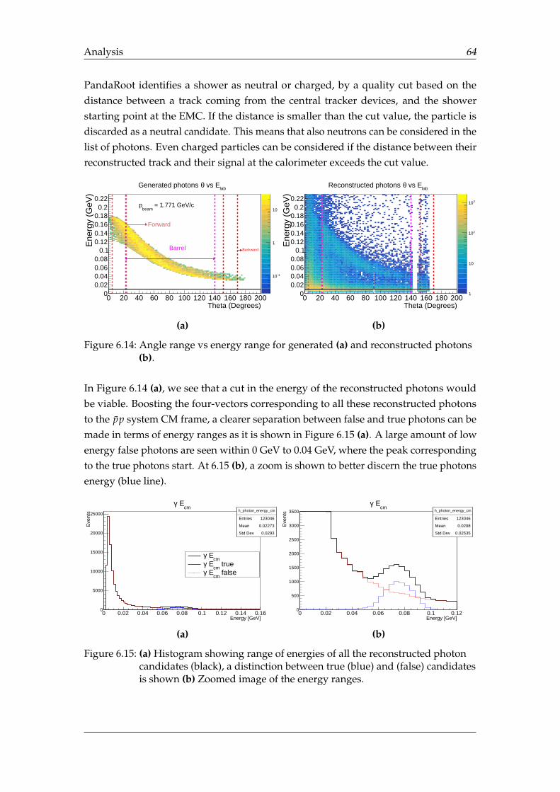
Analysis 64
PandaRoot identifies a shower as neutral or charged, by a quality cut based on thedistance between a track coming from the central tracker devices, and the showerstarting point at the EMC. If the distance is smaller than the cut value, the particle isdiscarded as a neutral candidate. This means that also neutrons can be considered in thelist of photons. Even charged particles can be considered if the distance between theirreconstructed track and their signal at the calorimeter exceeds the cut value.
Theta (Degrees)0 20 40 60 80 100 120 140 160 180 200
Ene
rgy
(GeV
)
00.020.040.060.08
0.10.120.140.160.180.2
0.22
1−10
1
10
Barrel
Forward
Backward
= 1.771 GeV/cbeam
p
lab vs EθGenerated photons
(a)
Theta (Degrees)0 20 40 60 80 100 120 140 160 180 200
Ene
rgy
(GeV
)0
0.020.040.060.08
0.10.120.140.160.180.2
0.22
1
10
210
310
lab vs EθReconstructed photons
(b)
Figure 6.14: Angle range vs energy range for generated (a) and reconstructed photons(b).
In Figure 6.14 (a), we see that a cut in the energy of the reconstructed photons wouldbe viable. Boosting the four-vectors corresponding to all these reconstructed photonsto the pp system CM frame, a clearer separation between false and true photons can bemade in terms of energy ranges as it is shown in Figure 6.15 (a). A large amount of lowenergy false photons are seen within 0 GeV to 0.04 GeV, where the peak correspondingto the true photons start. At 6.15 (b), a zoom is shown to better discern the true photonsenergy (blue line).
h_photon_energy_cm
Entries 123046
Mean 0.02273
Std Dev 0.0293
Energy [GeV]0 0.02 0.04 0.06 0.08 0.1 0.12 0.14 0.16
Eve
nts
0
5000
10000
15000
20000
25000h_photon_energy_cm
Entries 123046
Mean 0.02273
Std Dev 0.0293
cm Eγ
cm Eγ
truecm
Eγ false
cm Eγ
(a)
h_photon_energy_cm
Entries 123046
Mean 0.0208
Std Dev 0.02535
Energy [GeV]0 0.02 0.04 0.06 0.08 0.1 0.12
Eve
nts
0
500
1000
1500
2000
2500
3000
3500 h_photon_energy_cm
Entries 123046
Mean 0.0208
Std Dev 0.02535
cm Eγ
(b)
Figure 6.15: (a) Histogram showing range of energies of all the reconstructed photoncandidates (black), a distinction between true (blue) and (false) candidatesis shown (b) Zoomed image of the energy ranges.
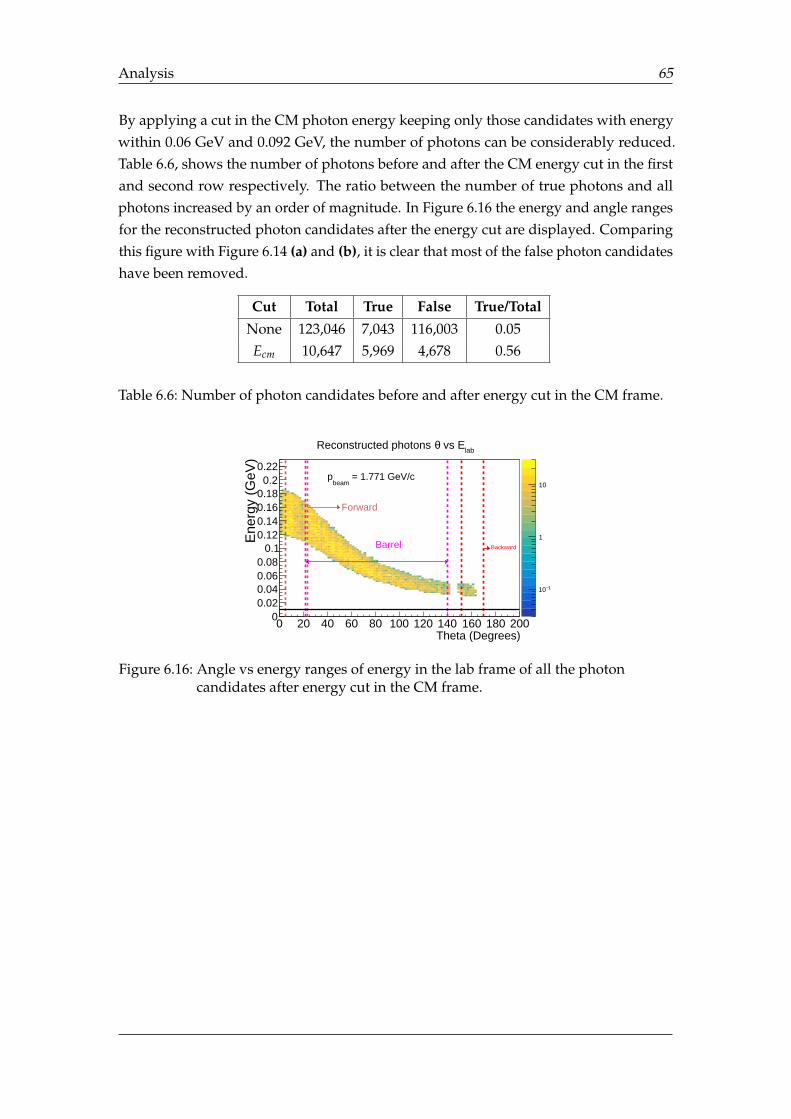
Analysis 65
By applying a cut in the CM photon energy keeping only those candidates with energywithin 0.06 GeV and 0.092 GeV, the number of photons can be considerably reduced.Table 6.6, shows the number of photons before and after the CM energy cut in the firstand second row respectively. The ratio between the number of true photons and allphotons increased by an order of magnitude. In Figure 6.16 the energy and angle rangesfor the reconstructed photon candidates after the energy cut are displayed. Comparingthis figure with Figure 6.14 (a) and (b), it is clear that most of the false photon candidateshave been removed.
Cut Total True False True/TotalNone 123,046 7,043 116,003 0.05Ecm 10,647 5,969 4,678 0.56
Table 6.6: Number of photon candidates before and after energy cut in the CM frame.
Theta (Degrees)0 20 40 60 80 100 120 140 160 180 200
Ene
rgy
(GeV
)
00.020.040.060.08
0.10.120.140.160.180.2
0.22
1−10
1
10
Barrel
Forward
Backward
= 1.771 GeV/cbeam
p
lab vs EθReconstructed photons
Figure 6.16: Angle vs energy ranges of energy in the lab frame of all the photoncandidates after energy cut in the CM frame.
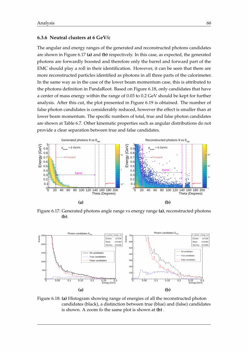
Analysis 66
6.3.6 Neutral clusters at 6 GeV/c
The angular and energy ranges of the generated and reconstructed photons candidatesare shown in Figure 6.17 (a) and (b) respectively. In this case, as expected, the generatedphotons are forwardly boosted and therefore only the barrel and forward part of theEMC should play a roll in their identification. However, it can be seen that there aremore reconstructed particles identified as photons in all three parts of the calorimeter.In the same way as in the case of the lower beam momentum case, this is attributed tothe photons definition in PandaRoot. Based on Figure 6.18, only candidates that havea center of mass energy within the range of 0.03 to 0.2 GeV should be kept for furtheranalysis. After this cut, the plot presented in Figure 6.19 is obtained. The number offalse photon candidates is considerably reduced, however the effect is smaller than atlower beam momentum. The specific numbers of total, true and false photon candidatesare shown at Table 6.7. Other kinematic properties such as angular distributions do notprovide a clear separation between true and false candidates.
Theta (Degrees)0 20 40 60 80 100 120 140 160 180 200
Ene
rgy
(GeV
)
0
0.1
0.2
0.3
0.4
0.5
0.6
0.7
0.8
0.91
1−10
1
10
Barrel
Forward
Backward
= 6 GeV/cbeam
p
lab vs EθGenerated photons
(a)
Theta (Degrees)0 20 40 60 80 100 120 140 160 180 200
Ene
rgy
(GeV
)
0
0.1
0.2
0.3
0.4
0.5
0.6
0.7
0.8
0.91
1
10
210
310
Barrel
Forward
Backward
= 6 GeV/cbeam
p
lab vs EθReconstructed photons
(b)
Figure 6.17: Generated photons angle range vs energy range (a), reconstructed photons(b).
h_photon_energy_cm
Entries 147240
Mean 0.02383
Std Dev 0.04206
Energy [GeV]0 0.05 0.1 0.15 0.2 0.25 0.3
Eve
nts
0
500
1000
1500
2000
2500 h_photon_energy_cm
Entries 147240
Mean 0.02383
Std Dev 0.04206
CMPhoton candidates E
All candidates
True candidates
False candidates
(a)
h_photon_energy_cm
Entries 147240
Mean 0.02383
Std Dev 0.04206
Energy [GeV]0 0.05 0.1 0.15 0.2 0.25 0.3
Eve
nts
0
100
200
300
400
500
600
700 h_photon_energy_cm
Entries 147240
Mean 0.02383
Std Dev 0.04206
CMPhoton candidates E
All candidates
True candidates
False candidates
(b)
Figure 6.18: (a) Histogram showing range of energies of all the reconstructed photoncandidates (black), a distinction between true (blue) and (false) candidatesis shown. A zoom fo the same plot is shown at (b) .
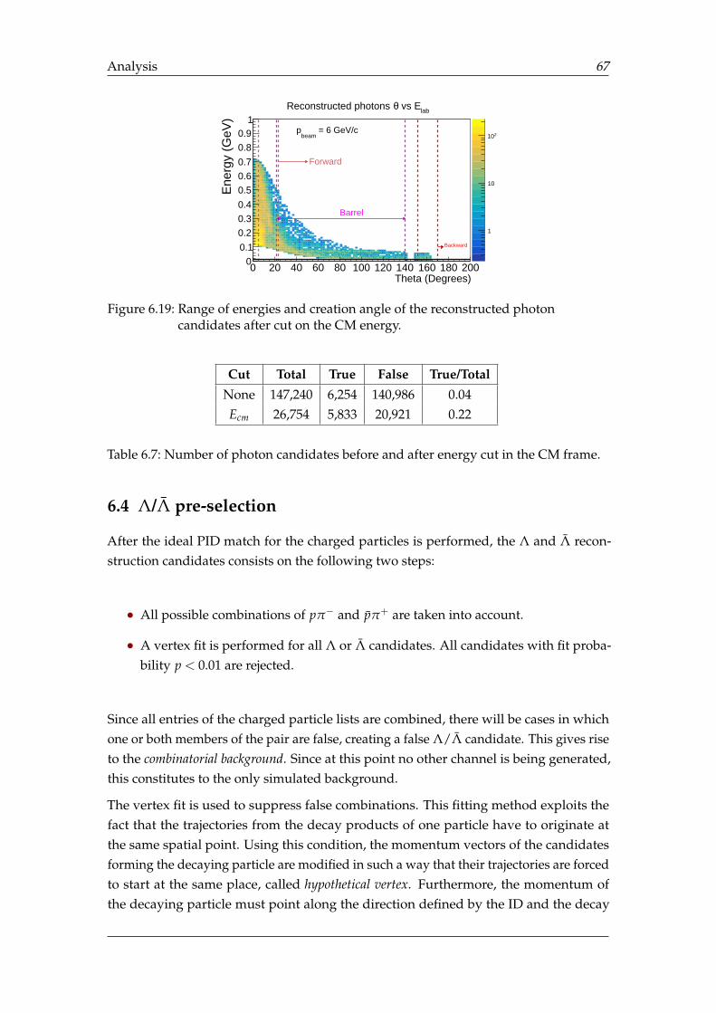
Analysis 67
Theta (Degrees)0 20 40 60 80 100 120 140 160 180 200
Ene
rgy
(GeV
)
0
0.1
0.2
0.3
0.4
0.5
0.6
0.7
0.8
0.91
1
10
210
Barrel
Forward
Backward
= 6 GeV/cbeam
p
lab vs EθReconstructed photons
Figure 6.19: Range of energies and creation angle of the reconstructed photoncandidates after cut on the CM energy.
Cut Total True False True/TotalNone 147,240 6,254 140,986 0.04Ecm 26,754 5,833 20,921 0.22
Table 6.7: Number of photon candidates before and after energy cut in the CM frame.
6.4 Λ/Λ pre-selection
After the ideal PID match for the charged particles is performed, the Λ and Λ recon-struction candidates consists on the following two steps:
• All possible combinations of pπ− and pπ+ are taken into account.
• A vertex fit is performed for all Λ or Λ candidates. All candidates with fit proba-bility p < 0.01 are rejected.
Since all entries of the charged particle lists are combined, there will be cases in whichone or both members of the pair are false, creating a false Λ/Λ candidate. This gives riseto the combinatorial background. Since at this point no other channel is being generated,this constitutes to the only simulated background.
The vertex fit is used to suppress false combinations. This fitting method exploits thefact that the trajectories from the decay products of one particle have to originate atthe same spatial point. Using this condition, the momentum vectors of the candidatesforming the decaying particle are modified in such a way that their trajectories are forcedto start at the same place, called hypothetical vertex. Furthermore, the momentum ofthe decaying particle must point along the direction defined by the ID and the decay
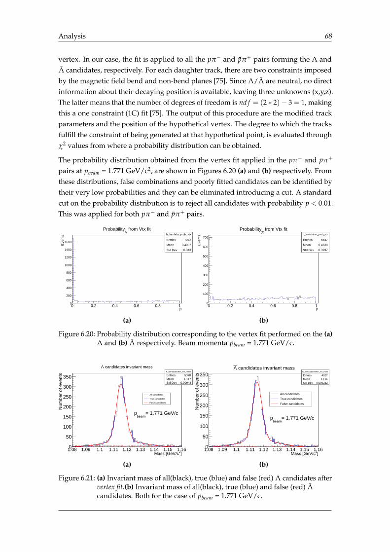
Analysis 68
vertex. In our case, the fit is applied to all the pπ− and pπ+ pairs forming the Λ andΛ candidates, respectively. For each daughter track, there are two constraints imposedby the magnetic field bend and non-bend planes [75]. Since Λ/Λ are neutral, no directinformation about their decaying position is available, leaving three unknowns (x,y,z).The latter means that the number of degrees of freedom is nd f = (2 ∗ 2)− 3 = 1, makingthis a one constraint (1C) fit [75]. The output of this procedure are the modified trackparameters and the position of the hypothetical vertex. The degree to which the tracksfulfill the constraint of being generated at that hypothetical point, is evaluated throughχ2 values from where a probability distribution can be obtained.
The probability distribution obtained from the vertex fit applied in the pπ− and pπ+
pairs at pbeam = 1.771 GeV/c2, are shown in Figures 6.20 (a) and (b) respectively. Fromthese distributions, false combinations and poorly fitted candidates can be identified bytheir very low probabilities and they can be eliminated introducing a cut. A standardcut on the probability distribution is to reject all candidates with probability p < 0.01.This was applied for both pπ− and pπ+ pairs.
h_lambda_prob_vtx
Entries 7072
Mean 0.4007
Std Dev 0.343
p0 0.2 0.4 0.6 0.8 1
Eve
nts
0
200
400
600
800
1000
1200
1400
1600
h_lambda_prob_vtx
Entries 7072
Mean 0.4007
Std Dev 0.343
from Vtx fitΛ
Probability
(a)
h_lambdabar_prob_vtx
Entries 5547
Mean 0.4738
Std Dev 0.3237
p0 0.2 0.4 0.6 0.8 1
Eve
nts
0
100
200
300
400
500
600
700h_lambdabar_prob_vtx
Entries 5547
Mean 0.4738
Std Dev 0.3237
from Vtx fitΛ
Probability
(b)
Figure 6.20: Probability distribution corresponding to the vertex fit performed on the (a)Λ and (b) Λ respectively. Beam momenta pbeam = 1.771 GeV/c.
h_lambdabetter_inv_mass
Entries 5378Mean 1.117Std Dev 0.00943
]2Mass [GeV/c1.08 1.09 1.1 1.11 1.12 1.13 1.14 1.15 1.16
Num
ber
of e
vent
s
0
50
100
150
200
250
300
350h_lambdabetter_inv_mass
Entries 5378Mean 1.117Std Dev 0.00943
All candidates
True candidates
False candidates
= 1.771 GeV/cbeam
p
candidates invariant massΛ
(a)
h_lambdabarbetter_inv_mass
Entries 4857Mean 1.116Std Dev 0.009232
]2Mass [GeV/c1.08 1.09 1.1 1.11 1.12 1.13 1.14 1.15 1.16
Num
ber
of e
vent
s
0
50
100
150
200
250
300
350h_lambdabarbetter_inv_mass
Entries 4857Mean 1.116Std Dev 0.009232
All candidates
True candidates
False candidates
= 1.771 GeV/cbeam
p
candidates invariant massΛ
(b)
Figure 6.21: (a) Invariant mass of all(black), true (blue) and false (red) Λ candidates aftervertex fit.(b) Invariant mass of all(black), true (blue) and false (red) Λcandidates. Both for the case of pbeam = 1.771 GeV/c.
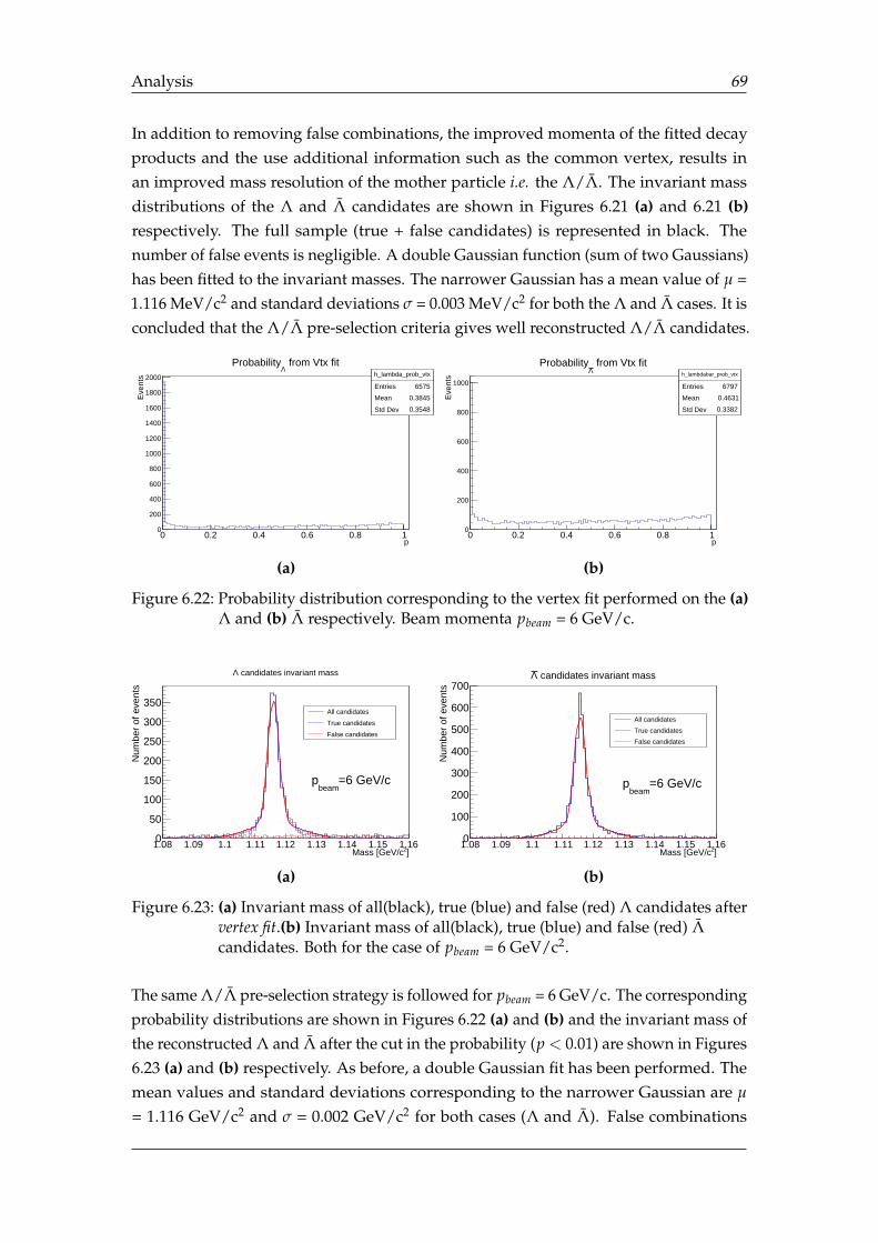
Analysis 69
In addition to removing false combinations, the improved momenta of the fitted decayproducts and the use additional information such as the common vertex, results inan improved mass resolution of the mother particle i.e. the Λ/Λ. The invariant massdistributions of the Λ and Λ candidates are shown in Figures 6.21 (a) and 6.21 (b)respectively. The full sample (true + false candidates) is represented in black. Thenumber of false events is negligible. A double Gaussian function (sum of two Gaussians)has been fitted to the invariant masses. The narrower Gaussian has a mean value of µ =1.116 MeV/c2 and standard deviations σ = 0.003 MeV/c2 for both the Λ and Λ cases. It isconcluded that the Λ/Λ pre-selection criteria gives well reconstructed Λ/Λ candidates.
h_lambda_prob_vtx
Entries 6575
Mean 0.3845
Std Dev 0.3548
p0 0.2 0.4 0.6 0.8 1
Eve
nts
0
200
400
600
800
1000
1200
1400
1600
1800
2000 h_lambda_prob_vtx
Entries 6575
Mean 0.3845
Std Dev 0.3548
from Vtx fitΛ
Probability
(a)
h_lambdabar_prob_vtx
Entries 6797
Mean 0.4631
Std Dev 0.3382
p0 0.2 0.4 0.6 0.8 1
Eve
nts
0
200
400
600
800
1000h_lambdabar_prob_vtx
Entries 6797
Mean 0.4631
Std Dev 0.3382
from Vtx fitΛ
Probability
(b)
Figure 6.22: Probability distribution corresponding to the vertex fit performed on the (a)Λ and (b) Λ respectively. Beam momenta pbeam = 6 GeV/c.
]2Mass [GeV/c1.08 1.09 1.1 1.11 1.12 1.13 1.14 1.15 1.16
Num
ber
of e
vent
s
0
50
100
150
200
250
300
350All candidates
True candidates
False candidates
=6 GeV/cbeam
p
candidates invariant massΛ
(a)
]2Mass [GeV/c1.08 1.09 1.1 1.11 1.12 1.13 1.14 1.15 1.16
Num
ber
of e
vent
s
0
100
200
300
400
500
600
700
All candidates
True candidates
False candidates
=6 GeV/cbeam
p
candidates invariant massΛ
(b)
Figure 6.23: (a) Invariant mass of all(black), true (blue) and false (red) Λ candidates aftervertex fit.(b) Invariant mass of all(black), true (blue) and false (red) Λcandidates. Both for the case of pbeam = 6 GeV/c2.
The same Λ/Λ pre-selection strategy is followed for pbeam = 6 GeV/c. The correspondingprobability distributions are shown in Figures 6.22 (a) and (b) and the invariant mass ofthe reconstructed Λ and Λ after the cut in the probability (p < 0.01) are shown in Figures6.23 (a) and (b) respectively. As before, a double Gaussian fit has been performed. Themean values and standard deviations corresponding to the narrower Gaussian are µ
= 1.116 GeV/c2 and σ = 0.002 GeV/c2 for both cases (Λ and Λ). False combinations
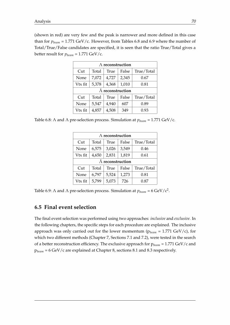
Analysis 70
(shown in red) are very few and the peak is narrower and more defined in this casethan for pbeam = 1.771 GeV/c. However, from Tables 6.8 and 6.9 where the number ofTotal/True/False candidates are specified, it is seen that the ratio True/Total gives abetter result for pbeam = 1.771 GeV/c.
Λ reconstructionCut Total True False True/Total
None 7,072 4,727 2,345 0.67
Vtx fit 5,378 4,368 1,010 0.81
Λ reconstructionCut Total True False True/Total
None 5,547 4,940 607 0.89
Vtx fit 4,857 4,508 349 0.93
Table 6.8: Λ and Λ pre-selection process. Simulation at pbeam = 1.771 GeV/c.
Λ reconstructionCut Total True False True/Total
None 6,575 3,026 3,549 0.46
Vtx fit 4,650 2,831 1,819 0.61
Λ reconstructionCut Total True False True/Total
None 6,797 5,524 1,273 0.81
Vtx fit 5,799 5,073 726 0.87
Table 6.9: Λ and Λ pre-selection process. Simulation at pbeam = 6 GeV/c2.
6.5 Final event selection
The final event selection was performed using two approaches: inclusive and exclusive. Inthe following chapters, the specific steps for each procedure are explained. The inclusiveapproach was only carried out for the lower momentum (pbeam = 1.771 GeV/c), forwhich two different methods (Chapter 7, Sections 7.1 and 7.2), were tested in the searchof a better reconstruction efficiency. The exclusive approach for pbeam = 1.771 GeV/c andpbeam = 6 GeV/c are explained at Chapter 8, sections 8.1 and 8.3 respectively.
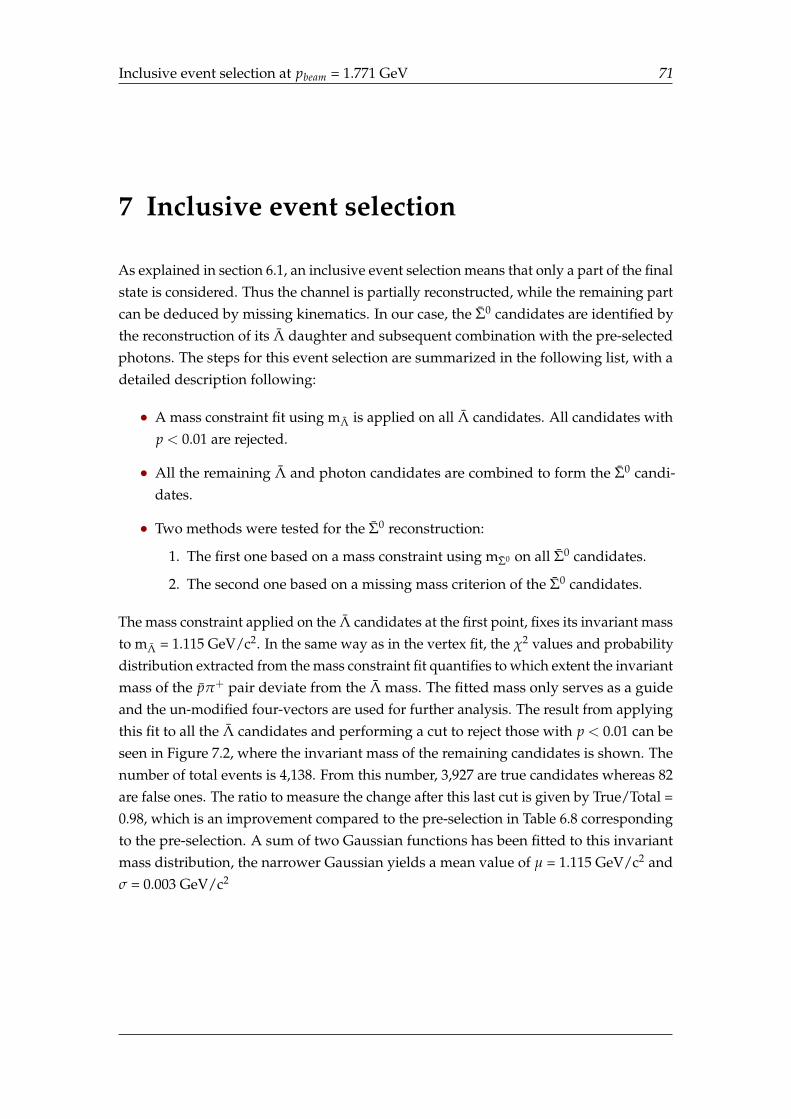
Inclusive event selection at pbeam = 1.771 GeV 71
7 Inclusive event selection
As explained in section 6.1, an inclusive event selection means that only a part of the finalstate is considered. Thus the channel is partially reconstructed, while the remaining partcan be deduced by missing kinematics. In our case, the Σ0 candidates are identified bythe reconstruction of its Λ daughter and subsequent combination with the pre-selectedphotons. The steps for this event selection are summarized in the following list, with adetailed description following:
• A mass constraint fit using mΛ is applied on all Λ candidates. All candidates withp < 0.01 are rejected.
• All the remaining Λ and photon candidates are combined to form the Σ0 candi-dates.
• Two methods were tested for the Σ0 reconstruction:
1. The first one based on a mass constraint using mΣ0 on all Σ0 candidates.
2. The second one based on a missing mass criterion of the Σ0 candidates.
The mass constraint applied on the Λ candidates at the first point, fixes its invariant massto mΛ = 1.115 GeV/c2. In the same way as in the vertex fit, the χ2 values and probabilitydistribution extracted from the mass constraint fit quantifies to which extent the invariantmass of the pπ+ pair deviate from the Λ mass. The fitted mass only serves as a guideand the un-modified four-vectors are used for further analysis. The result from applyingthis fit to all the Λ candidates and performing a cut to reject those with p < 0.01 can beseen in Figure 7.2, where the invariant mass of the remaining candidates is shown. Thenumber of total events is 4,138. From this number, 3,927 are true candidates whereas 82are false ones. The ratio to measure the change after this last cut is given by True/Total =0.98, which is an improvement compared to the pre-selection in Table 6.8 correspondingto the pre-selection. A sum of two Gaussian functions has been fitted to this invariantmass distribution, the narrower Gaussian yields a mean value of µ = 1.115 GeV/c2 andσ = 0.003 GeV/c2
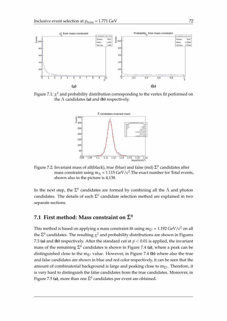
Inclusive event selection at pbeam = 1.771 GeV 72
h_lambdabar_chi2_mass
Entries 5547
Mean 1.405
Std Dev 1.985
2χ0 1 2 3 4 5 6 7 8 9 10
Eve
nts
0
200
400
600
800
1000
h_lambdabar_chi2_mass
Entries 5547
Mean 1.405
Std Dev 1.985
from mass constraintΛ2χ
(a)
h_lambdabar_prob_mass
Entries 5547
Mean 0.3884
Std Dev 0.3289
p0 0.2 0.4 0.6 0.8 1
Eve
nts
0
200
400
600
800
1000
h_lambdabar_prob_mass
Entries 5547
Mean 0.3884
Std Dev 0.3289
from mass constraintΛ
Probability
(b)
Figure 7.1: χ2 and probability distribution corresponding to the vertex fit performed onthe Λ candidates (a) and (b) respectively.
h_lambdabarbetter_inv_massEntries 4138Mean 1.116Std Dev 0.006697Prob 0.05124p0 7.9± 287.5 p1 0.000± 1.115 p2 0.000120± 0.003395 p3 7.76± 28.21 p4 0.001± 1.117 p5 0.001050± 0.009098
]2Mass[GeV/c1.08 1.09 1.1 1.11 1.12 1.13 1.14 1.15 1.16
Eve
nts
0
50
100
150
200
250
300
350
h_lambdabarbetter_inv_massEntries 4138Mean 1.116Std Dev 0.006697Prob 0.05124p0 7.9± 287.5 p1 0.000± 1.115 p2 0.000120± 0.003395 p3 7.76± 28.21 p4 0.001± 1.117 p5 0.001050± 0.009098
candidates invariant massΛ
Figure 7.2: Invariant mass of all(black), true (blue) and false (red) Σ0 candidates aftermass constraint using mΛ = 1.115 GeV/c2.The exact number for Total events,shown also in the picture is 4,138.
In the next step, the Σ0 candidates are formed by combining all the Λ and photoncandidates. The details of each Σ0 candidate selection method are explained in twoseparate sections.
7.1 First method: Mass constraint on Σ0
This method is based on applying a mass constraint fit using mΣ0 = 1.192 GeV/c2 on allthe Σ0 candidates. The resulting χ2 and probability distributions are shown in Figures7.3 (a) and (b) respectively. After the standard cut at p < 0.01 is applied, the invariantmass of the remaining Σ0 candidates is shown in Figure 7.4 (a), where a peak can bedistinguished close to the mΣ0 value. However, in Figure 7.4 (b) where also the trueand false candidates are shown in blue and red color respectively, it can be seen that theamount of combinatorial background is large and peaking close to mΣ0 . Therefore, itis very hard to distinguish the false candidates from the true candidates. Moreover, inFigure 7.5 (a), more than one Σ0 candidates per event are obtained.
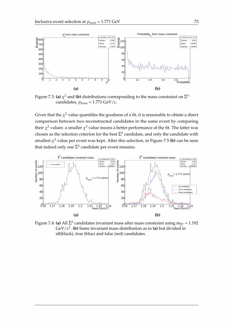
Inclusive event selection at pbeam = 1.771 GeV 73
h_sigmabar_chi2_mass
Entries 3709
Mean 1.275
Std Dev 1.561
2χ0 1 2 3 4 5 6 7 8 9 10
Eve
nts
0
100
200
300
400
500
600
700
800h_sigmabar_chi2_mass
Entries 3709
Mean 1.275
Std Dev 1.561
from mass constraintΣ2χ
(a)
h_sigmabar_prob_mass
Entries 3709
Mean 0.4509
Std Dev 0.2999
Probability0 0.2 0.4 0.6 0.8 1
Eve
nts
0
20
40
60
80
100
120
h_sigmabar_prob_mass
Entries 3709
Mean 0.4509
Std Dev 0.2999
from mass constraintΣ
Probability
(b)
Figure 7.3: (a) χ2 and (b) distributions corresponding to the mass constraint on Σ0
candidates, pbeam = 1.771 GeV/c.
Given that the χ2 value quantifies the goodness of a fit, it is reasonable to obtain a directcomparison between two reconstructed candidates in the same event by comparingtheir χ2 values: a smaller χ2 value means a better performance of the fit. The latter waschosen as the selection criterion for the best Σ0 candidate, and only the candidate withsmallest χ2 value per event was kept. After this selection, in Figure 7.5 (b) can be seenthat indeed only one Σ0 candidate per event remains.
h_sigmabarbetter_mass
Entries 3709Mean 1.192Std Dev 0.008883
]2Mass [GeV/c1.16 1.17 1.18 1.19 1.2 1.21 1.22 1.23
Num
ber
of e
vent
s
0
20
40
60
80
100
120
h_sigmabarbetter_mass
Entries 3709Mean 1.192Std Dev 0.008883
All candidates
= 1.771 GeV/cbeam
p
candidates invariant mass0
Σ
(a)
h_sigmabarbetter_mass
Entries 3709Mean 1.192Std Dev 0.008883
]2Mass [GeV/c1.16 1.17 1.18 1.19 1.2 1.21 1.22 1.23
Num
ber
of e
vent
s
0
20
40
60
80
100
120
h_sigmabarbetter_mass
Entries 3709Mean 1.192Std Dev 0.008883
All candidates
True candidates
False candidates
= 1.771 GeV/cbeam
p
candidates invariant mass0
Σ
(b)
Figure 7.4: (a) All Σ0 candidates invariant mass after mass constraint using mΣ0 = 1.192GeV/c2. (b) Same invariant mass distribution as in (a) but divided inall(black), true (blue) and false (red) candidates.
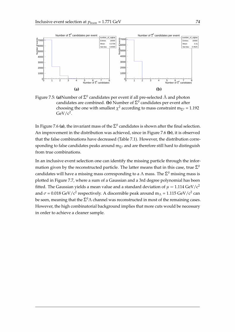
Inclusive event selection at pbeam = 1.771 GeV 74
number_of_sigbar
Entries 10000
Mean 0.3709
Std Dev 0.6569
candidates0
ΣNumber of 0 1 2 3 4 5 6 7 8
Num
ber
of e
vent
s
0
1000
2000
3000
4000
5000
6000
7000number_of_sigbar
Entries 10000
Mean 0.3709
Std Dev 0.6569
candidates per event0
ΣNumber of
(a)
number_of_sigbar
Entries 10000
Mean 0.31
Std Dev 0.4625
candidates0
ΣNumber of 0 1 2 3 4 5 6 7 8
Num
ber
of e
vent
s
0
1000
2000
3000
4000
5000
6000
7000number_of_sigbar
Entries 10000
Mean 0.31
Std Dev 0.4625
candidates per event0
ΣNumber of
(b)
Figure 7.5: (a)Number of Σ0 candidates per event if all pre-selected Λ and photoncandidates are combined. (b) Number of Σ0 candidates per event afterchoosing the one with smallest χ2 according to mass constraint mΣ0 = 1.192GeV/c2.
In Figure 7.6 (a), the invariant mass of the Σ0 candidates is shown after the final selection.An improvement in the distribution was achieved, since in Figure 7.6 (b), it is observedthat the false combinations have decreased (Table 7.1). However, the distribution corre-sponding to false candidates peaks around mΣ0 and are therefore still hard to distinguishfrom true combinations.
In an inclusive event selection one can identify the missing particle through the infor-mation given by the reconstructed particle. The latter means that in this case, true Σ0
candidates will have a missing mass corresponding to a Λ mass. The Σ0 missing mass isplotted in Figure 7.7, where a sum of a Gaussian and a 3rd degree polynomial has beenfitted. The Gaussian yields a mean value and a standard deviation of µ = 1.114 GeV/c2
and σ = 0.018 GeV/c2 respectively. A discernible peak around mΛ = 1.115 GeV/c2 canbe seen, meaning that the Σ0Λ channel was reconstructed in most of the remaining cases.However, the high combinatorial background implies that more cuts would be necessaryin order to achieve a cleaner sample.
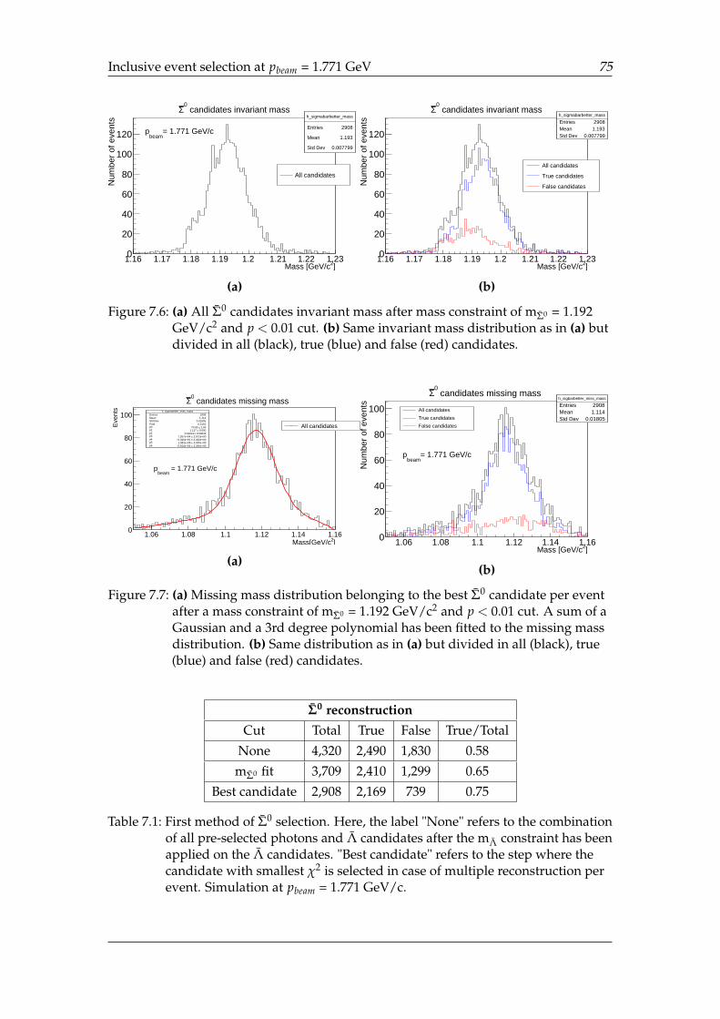
Inclusive event selection at pbeam = 1.771 GeV 75
h_sigmabarbetter_mass
Entries 2908
Mean 1.193
Std Dev 0.007799
]2Mass [GeV/c1.16 1.17 1.18 1.19 1.2 1.21 1.22 1.23
Num
ber
of e
vent
s
0
20
40
60
80
100
120
h_sigmabarbetter_mass
Entries 2908
Mean 1.193
Std Dev 0.007799
All candidates
= 1.771 GeV/cbeam
p
candidates invariant mass0
Σ
(a)
h_sigmabarbetter_mass
Entries 2908Mean 1.193Std Dev 0.007799
]2Mass [GeV/c1.16 1.17 1.18 1.19 1.2 1.21 1.22 1.23
Num
ber
of e
vent
s
0
20
40
60
80
100
120
h_sigmabarbetter_mass
Entries 2908Mean 1.193Std Dev 0.007799
All candidates
True candidates
False candidates
= 1.771 GeV/cbeam
p
candidates invariant mass0
Σ
(b)
Figure 7.6: (a) All Σ0 candidates invariant mass after mass constraint of mΣ0 = 1.192GeV/c2 and p < 0.01 cut. (b) Same invariant mass distribution as in (a) butdivided in all (black), true (blue) and false (red) candidates.
h_sigmabetter_miss_massEntries 2908Mean 1.114Std Dev 0.01805Prob 0.3153p0 2.60± 70.83 p1 0.000± 1.117 p2 0.00033± 0.01021 p3 2.972e+00± 7.267e+04 p4 3.330e+00±2.026e+05 − p5 3.040e+00± 1.881e+05 p6 2.240e+00±5.814e+04 −
]2Mass[GeV/c1.06 1.08 1.1 1.12 1.14 1.16
Eve
nts
0
20
40
60
80
100h_sigmabetter_miss_mass
Entries 2908Mean 1.114Std Dev 0.01805Prob 0.3153p0 2.60± 70.83 p1 0.000± 1.117 p2 0.00033± 0.01021 p3 2.972e+00± 7.267e+04 p4 3.330e+00±2.026e+05 − p5 3.040e+00± 1.881e+05 p6 2.240e+00±5.814e+04 −
candidates missing mass0Σ
All candidates
= 1.771 GeV/cbeam
p
(a)
h_sigbarbetter_miss_mass
Entries 2908Mean 1.114Std Dev 0.01805
]2Mass [GeV/c1.06 1.08 1.1 1.12 1.14 1.16
Num
ber
of e
vent
s
0
20
40
60
80
100h_sigbarbetter_miss_mass
Entries 2908Mean 1.114Std Dev 0.01805
All candidates
True candidates
False candidates
= 1.771 GeV/cbeam
p
candidates missing mass 0
Σ
(b)
Figure 7.7: (a) Missing mass distribution belonging to the best Σ0 candidate per eventafter a mass constraint of mΣ0 = 1.192 GeV/c2 and p < 0.01 cut. A sum of aGaussian and a 3rd degree polynomial has been fitted to the missing massdistribution. (b) Same distribution as in (a) but divided in all (black), true(blue) and false (red) candidates.
Σ0 reconstructionCut Total True False True/Total
None 4,320 2,490 1,830 0.58
mΣ0 fit 3,709 2,410 1,299 0.65
Best candidate 2,908 2,169 739 0.75
Table 7.1: First method of Σ0 selection. Here, the label "None" refers to the combinationof all pre-selected photons and Λ candidates after the mΛ constraint has beenapplied on the Λ candidates. "Best candidate" refers to the step where thecandidate with smallest χ2 is selected in case of multiple reconstruction perevent. Simulation at pbeam = 1.771 GeV/c.
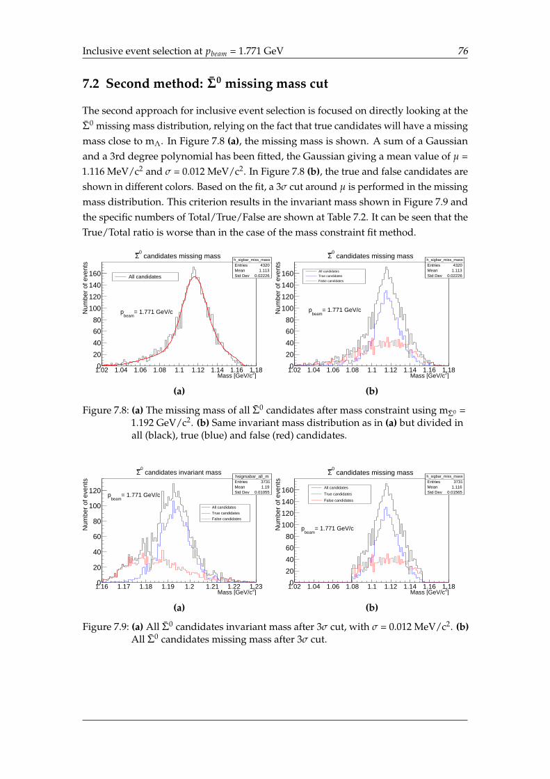
Inclusive event selection at pbeam = 1.771 GeV 76
7.2 Second method: Σ0 missing mass cut
The second approach for inclusive event selection is focused on directly looking at theΣ0 missing mass distribution, relying on the fact that true candidates will have a missingmass close to mΛ. In Figure 7.8 (a), the missing mass is shown. A sum of a Gaussianand a 3rd degree polynomial has been fitted, the Gaussian giving a mean value of µ =1.116 MeV/c2 and σ = 0.012 MeV/c2. In Figure 7.8 (b), the true and false candidates areshown in different colors. Based on the fit, a 3σ cut around µ is performed in the missingmass distribution. This criterion results in the invariant mass shown in Figure 7.9 andthe specific numbers of Total/True/False are shown at Table 7.2. It can be seen that theTrue/Total ratio is worse than in the case of the mass constraint fit method.
h_sigbar_miss_massEntries 4320Mean 1.113Std Dev 0.02226
]2Mass [GeV/c1.02 1.04 1.06 1.08 1.1 1.12 1.14 1.16 1.18
Num
ber
of e
vent
s
0
20
40
60
80
100
120
140
160
h_sigbar_miss_massEntries 4320Mean 1.113Std Dev 0.02226All candidates
= 1.771 GeV/cbeam
p
candidates missing mass 0
Σ
(a)
h_sigbar_miss_massEntries 4320Mean 1.113Std Dev 0.02226
]2Mass [GeV/c1.02 1.04 1.06 1.08 1.1 1.12 1.14 1.16 1.18
Num
ber
of e
vent
s
0
20
40
60
80
100
120
140
160
h_sigbar_miss_massEntries 4320Mean 1.113Std Dev 0.02226
All candidatesTrue candidates
False candidates
= 1.771 GeV/cbeam
p
candidates missing mass 0
Σ
(b)
Figure 7.8: (a) The missing mass of all Σ0 candidates after mass constraint using mΣ0 =1.192 GeV/c2. (b) Same invariant mass distribution as in (a) but divided inall (black), true (blue) and false (red) candidates.
hsigmabar_all_mEntries 3731Mean 1.19Std Dev 0.01055
]2Mass [GeV/c1.16 1.17 1.18 1.19 1.2 1.21 1.22 1.23
Num
ber
of e
vent
s
0
20
40
60
80
100
120
hsigmabar_all_mEntries 3731Mean 1.19Std Dev 0.01055
All candidates
True candidates
False candidates
= 1.771 GeV/cbeam
p
candidates invariant mass0
Σ
(a)
h_sigbar_miss_massEntries 3731Mean 1.116Std Dev 0.01565
]2Mass [GeV/c1.02 1.04 1.06 1.08 1.1 1.12 1.14 1.16 1.18
Num
ber
of e
vent
s
0
20
40
60
80
100
120
140
160
h_sigbar_miss_massEntries 3731Mean 1.116Std Dev 0.01565
All candidates
True candidates
False candidates
= 1.771 GeV/cbeam
p
candidates missing mass 0
Σ
(b)
Figure 7.9: (a) All Σ0 candidates invariant mass after 3σ cut, with σ = 0.012 MeV/c2. (b)All Σ0 candidates missing mass after 3σ cut.
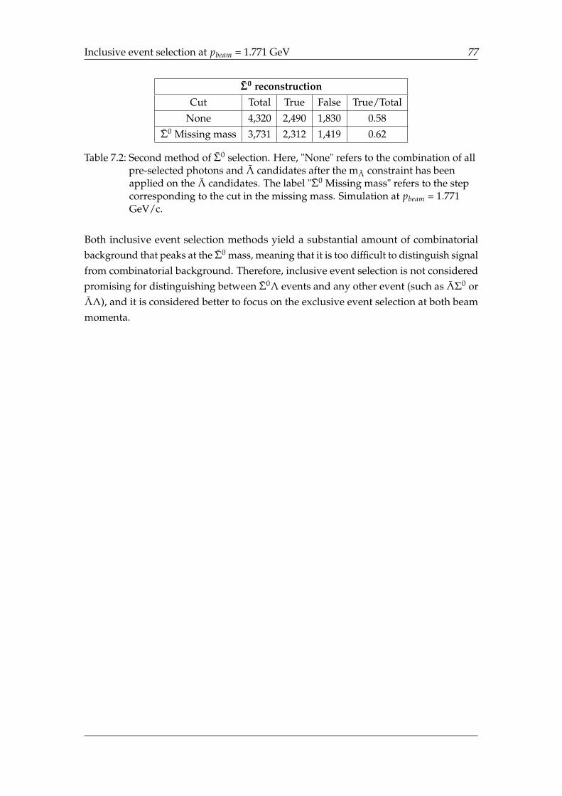
Inclusive event selection at pbeam = 1.771 GeV 77
Σ0 reconstructionCut Total True False True/Total
None 4,320 2,490 1,830 0.58
Σ0 Missing mass 3,731 2,312 1,419 0.62
Table 7.2: Second method of Σ0 selection. Here, "None" refers to the combination of allpre-selected photons and Λ candidates after the mΛ constraint has beenapplied on the Λ candidates. The label "Σ0 Missing mass" refers to the stepcorresponding to the cut in the missing mass. Simulation at pbeam = 1.771GeV/c.
Both inclusive event selection methods yield a substantial amount of combinatorialbackground that peaks at the Σ0 mass, meaning that it is too difficult to distinguish signalfrom combinatorial background. Therefore, inclusive event selection is not consideredpromising for distinguishing between Σ0Λ events and any other event (such as ΛΣ0 orΛΛ), and it is considered better to focus on the exclusive event selection at both beammomenta.
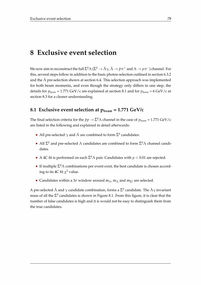
Exclusive event selection 78
8 Exclusive event selection
We now aim to reconstruct the full Σ0Λ (Σ0→ Λγ, Λ→ pπ+ and Λ→ pπ−) channel. Forthis, several steps follow in addition to the basic photon selection outlined in section 6.3.2and the Λ pre-selection shown at section 6.4. This selection approach was implementedfor both beam momenta, and even though the strategy only differs in one step, thedetails for pbeam = 1.771 GeV/c are explained at section 8.1 and for pbeam = 6 GeV/c atsection 8.3 for a clearer understanding.
8.1 Exclusive event selection at pbeam = 1.771 GeV/c
The final selection criteria for the pp→ Σ0Λ channel in the case of pbeam = 1.771 GeV/care listed in the following and explained in detail afterwards:
• All pre-selected γ and Λ are combined to form Σ0 candidates.
• All Σ0 and pre-selected Λ candidates are combined to form Σ0Λ channel candi-dates.
• A 4C fit is performed on each Σ0Λ pair. Candidates with p < 0.01 are rejected.
• If multiple Σ0Λ combinations per event exist, the best candidate is chosen accord-ing to its 4C fit χ2 value.
• Candidates within a 3σ window around mΛ, mΛ and mΣ0 are selected.
A pre-selected Λ and γ candidate combination, forms a Σ0 candidate. The Λγ invariantmass of all the Σ0 candidates is shown in Figure 8.1. From this figure, it is clear that thenumber of false candidates is high and it is would not be easy to distinguish them fromthe true candidates.
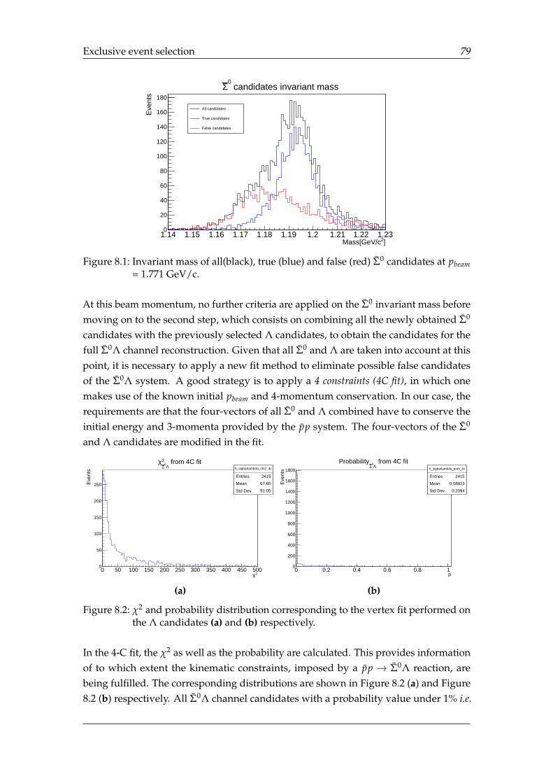
Exclusive event selection 79
]2Mass[GeV/c1.14 1.15 1.16 1.17 1.18 1.19 1.2 1.21 1.22 1.23
Eve
nts
0
20
40
60
80
100
120
140
160
180
candidates invariant mass0
Σ
All candidates
True candidates
False candidates
Figure 8.1: Invariant mass of all(black), true (blue) and false (red) Σ0 candidates at pbeam= 1.771 GeV/c.
At this beam momentum, no further criteria are applied on the Σ0 invariant mass beforemoving on to the second step, which consists on combining all the newly obtained Σ0
candidates with the previously selected Λ candidates, to obtain the candidates for thefull Σ0Λ channel reconstruction. Given that all Σ0 and Λ are taken into account at thispoint, it is necessary to apply a new fit method to eliminate possible false candidatesof the Σ0Λ system. A good strategy is to apply a 4 constraints (4C fit), in which onemakes use of the known initial pbeam and 4-momentum conservation. In our case, therequirements are that the four-vectors of all Σ0 and Λ combined have to conserve theinitial energy and 3-momenta provided by the pp system. The four-vectors of the Σ0
and Λ candidates are modified in the fit.
h_sigbarlambda_chi2_4c
Entries 2415
Mean 67.65
Std Dev 91.05
2χ0 50 100 150 200 250 300 350 400 450 500
Eve
nts
0
50
100
150
200
250
h_sigbarlambda_chi2_4c
Entries 2415
Mean 67.65
Std Dev 91.05
from 4C fitΛ
0Σ2χ
(a)
h_sigbarlambda_prob_4c
Entries 2415
Mean 0.08823
Std Dev 0.2094
p0 0.2 0.4 0.6 0.8 1
Eve
nts
0
200
400
600
800
1000
1200
1400
1600
1800 h_sigbarlambda_prob_4c
Entries 2415
Mean 0.08823
Std Dev 0.2094
from 4C fitΛ
0Σ
Probability
(b)
Figure 8.2: χ2 and probability distribution corresponding to the vertex fit performed onthe Λ candidates (a) and (b) respectively.
In the 4-C fit, the χ2 as well as the probability are calculated. This provides informationof to which extent the kinematic constraints, imposed by a pp → Σ0Λ reaction, arebeing fulfilled. The corresponding distributions are shown in Figure 8.2 (a) and Figure8.2 (b) respectively. All Σ0Λ channel candidates with a probability value under 1% i.e.
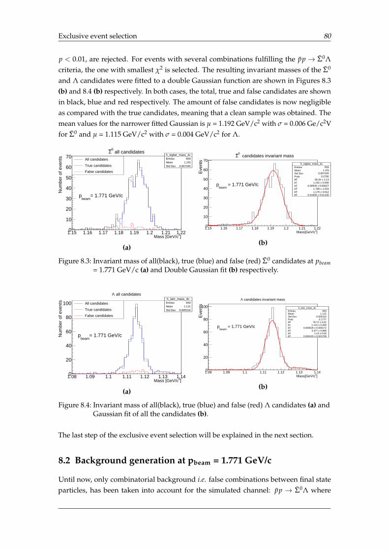
Exclusive event selection 80
p < 0.01, are rejected. For events with several combinations fulfilling the pp→ Σ0Λcriteria, the one with smallest χ2 is selected. The resulting invariant masses of the Σ0
and Λ candidates were fitted to a double Gaussian function are shown in Figures 8.3(b) and 8.4 (b) respectively. In both cases, the total, true and false candidates are shownin black, blue and red respectively. The amount of false candidates is now negligibleas compared with the true candidates, meaning that a clean sample was obtained. Themean values for the narrower fitted Gaussian is µ = 1.192 GeV/c2 with σ = 0.006 Ge/c2Vfor Σ0 and µ = 1.115 GeV/c2 with σ = 0.004 GeV/c2 for Λ.
h_sigbar_mass_4cEntries 659Mean 1.191Std Dev 0.007345
]2Mass [GeV/c1.15 1.16 1.17 1.18 1.19 1.2 1.21 1.22
Num
ber
of e
vent
s
0
10
20
30
40
50
60
70 h_sigbar_mass_4cEntries 659Mean 1.191Std Dev 0.007345
All candidates
True candidates
False candidates
= 1.771 GeV/cbeam
p
all candidates0Σ
(a)
h_sigbar_mass_4cEntries 659Mean 1.191Std Dev 0.007345Prob 0.2795p0 3.13± 58.26 p1 0.000± 1.192 p2 0.00027± 0.00549 p3 1.010± 1.799 p4 0.012± 1.178 p5 0.01100± 0.01839
]2Mass[GeV/c1.15 1.16 1.17 1.18 1.19 1.2 1.21 1.22
Eve
nts
0
10
20
30
40
50
60
70h_sigbar_mass_4c
Entries 659Mean 1.191Std Dev 0.007345Prob 0.2795p0 3.13± 58.26 p1 0.000± 1.192 p2 0.00027± 0.00549 p3 1.010± 1.799 p4 0.012± 1.178 p5 0.01100± 0.01839
candidates invariant mass0
Σ
= 1.771 GeV/cbeam
p
(b)
Figure 8.3: Invariant mass of all(black), true (blue) and false (red) Σ0 candidates at pbeam= 1.771 GeV/c (a) and Double Gaussian fit (b) respectively.
h_lam_mass_4cEntries 659Mean 1.115Std Dev 0.005316
]2Mass [GeV/c1.08 1.09 1.1 1.11 1.12 1.13 1.14
Num
ber
of e
vent
s
0
20
40
60
80
100h_lam_mass_4c
Entries 659Mean 1.115Std Dev 0.005316
All candidates
True candidates
False candidates
= 1.771 GeV/cbeam
p
all candidatesΛ
(a)
h_lam_mass_4cEntries 659Mean 1.115Std Dev 0.005316Prob 0.1777p0 4.62± 78.72 p1 0.000± 1.115 p2 0.000172± 0.003626 p3 0.898± 3.377 p4 0.00± 1.13 p5 0.001708± 0.004193
]2Mass[GeV/c1.08 1.09 1.1 1.11 1.12 1.13 1.14
Eve
nts
0
20
40
60
80
100 h_lam_mass_4cEntries 659Mean 1.115Std Dev 0.005316Prob 0.1777p0 4.62± 78.72 p1 0.000± 1.115 p2 0.000172± 0.003626 p3 0.898± 3.377 p4 0.00± 1.13 p5 0.001708± 0.004193
candidates invariant massΛ
= 1.771 GeV/cbeam
p
(b)
Figure 8.4: Invariant mass of all(black), true (blue) and false (red) Λ candidates (a) andGaussian fit of all the candidates (b).
The last step of the exclusive event selection will be explained in the next section.
8.2 Background generation at pbeam = 1.771 GeV/c
Until now, only combinatorial background i.e. false combinations between final stateparticles, has been taken into account for the simulated channel: pp → Σ0Λ where
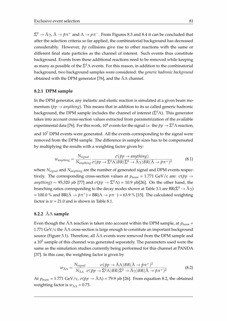
Exclusive event selection 81
Σ0→ Λγ, Λ→ pπ+ and Λ→ pπ−. From Figures 8.3 and 8.4 it can be concluded thatafter the selection criteria so far applied, the combinatorial background has decreasedconsiderably. However, pp collisions give rise to other reactions with the same ordifferent final state particles as the channel of interest. Such events thus constitutebackground. Events from these additional reactions need to be removed while keepingas many as possible of the Σ0Λ events. For this reason, in addition to the combinatorialbackground, two background samples were considered: the generic hadronic backgroundobtained with the DPM generator [76], and the ΛΛ channel.
8.2.1 DPM sample
In the DPM generator, any inelastic and elastic reaction is simulated at a given beam mo-mentum (pp→ anything). This means that in addition to its so called generic hadronicbackground, the DPM sample includes the channel of interest (Σ0Λ). This generatortakes into account cross-section values extracted from parametrization of the availableexperimental data [76]. For this work, 104 events for the signal i.e. the pp→ Σ0Λ reaction,
and 107 DPM events were generated. All the events corresponding to the signal wereremoved from the DPM sample. The difference in sample sizes has to be compensatedby multiplying the results with a weighting factor given by:
wanything =Nsignal
Nanything
σ( pp→ anything)σ( pp→ Σ0Λ)BR(Σ0→ Λγ)BR(Λ→ pπ+)2 (8.1)
where Nsignal and Nanything are the number of generated signal and DPM events respec-tively. The corresponding cross-section values at pbeam = 1.771 GeV/c are: σ(pp →anything) ∼ 95,320 µb [77] and σ(pp → Σ0Λ) = 10.9 µb[26]. On the other hand, thebranching ratios corresponding to the decay modes shown at Table 3.1 are BR(Σ0→ Λγ)= 100.0 % and BR(Λ→ pπ+) = BR(Λ→ pπ−) = 63.9 % [15]. The calculated weightingfactor is w = 21.0 and is shown in Table 8.1.
8.2.2 ΛΛ sample
Even though the ΛΛ reaction is taken into account within the DPM sample, at pbeam =1.771 GeV/c the ΛΛ cross-section is large enough to constitute an important backgroundsource (Figure 3.1). Therefore, all ΛΛ events were removed from the DPM sample anda 105 sample of this channel was generated separately. The parameters used were thesame as the simulation studies currently being performed for this channel at PANDA[37]. In this case, the weighting factor is given by
wΛΛ =Nsignal
NΛΛ
σ( pp→ ΛΛ)BR(Λ→ pπ+)2
σ( pp→ Σ0Λ)BR(Σ0→ Λγ)BR(Λ→ pπ+)2 (8.2)
At pbeam = 1.771 GeV/c, σ(pp→ ΛΛ) = 79.9 µb [26]. From equation 8.2, the obtainedweighting factor is wΛΛ = 0.73.
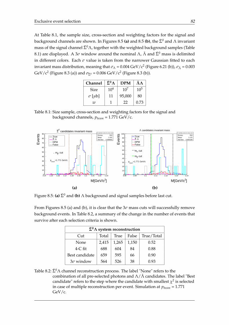
Exclusive event selection 82
At Table 8.1, the sample size, cross-section and weighting factors for the signal andbackground channels are shown. In Figures 8.5 (a) and 8.5 (b), the Σ0 and Λ invariantmass of the signal channel Σ0Λ, together with the weighted background samples (Table8.1) are displayed. A 3σ window around the nominal Λ, Λ and Σ0 mass is delimitedin different colors. Each σ value is taken from the narrower Gaussian fitted to eachinvariant mass distribution, meaning that σΛ = 0.004 GeV/c2 (Figure 6.21 (b)), σΛ = 0.003GeV/c2 (Figure 8.3 (a)) and σΣ0 = 0.006 GeV/c2 (Figure 8.3 (b)).
Channel Σ0Λ DPM ΛΛ
Size 104 107 105
σ [µb] 11 95,000 80w 1 22 0.73
Table 8.1: Size sample, cross-section and weighting factors for the signal andbackground channels, pbeam = 1.771 GeV/c.
h_sigmabar_cand_inv_mass_true
Entries 593Mean 1.192Std Dev 0.006691
]2M[GeV/c
1.14 1.15 1.16 1.17 1.18 1.19 1.2 1.21 1.22 1.23
Eve
nts
0
10
20
30
40
50
60
70
80
90h_sigmabar_cand_inv_mass_true
Entries 593Mean 1.192Std Dev 0.006691
=1.771 GeV/cbeam
p
TrueΛ Λ
DPMFalse
cut0Σ
m
candidates invariant mass0
Σ
(a)
h_lambda_cand_inv_mass_true
Entries 593Mean 1.115Std Dev 0.005168
]2M[GeV/c
1.08 1.09 1.1 1.11 1.12 1.13 1.14
Eve
nts
0
10
20
30
40
50
60
70
80
90
100h_lambda_cand_inv_mass_true
Entries 593Mean 1.115Std Dev 0.005168
=1.771 GeV/cbeam
p
TrueΛ Λ
DPMFalse
cutΛm
cutΛm
candidates invariant massΛ
(b)
Figure 8.5: (a) Σ0 and (b) Λ background and signal samples before last cut.
From Figures 8.5 (a) and (b), it is clear that the 3σ mass cuts will successfully removebackground events. In Table 8.2, a summary of the change in the number of events thatsurvive after each selection criteria is shown.
Σ0Λ system reconstructionCut Total True False True/Total
None 2,415 1,265 1,150 0.524-C fit 688 604 84 0.88
Best candidate 659 595 66 0.903σ window 564 526 38 0.93
Table 8.2: Σ0Λ channel reconstruction process. The label "None" refers to thecombination of all pre-selected photons and Λ/Λ candidates. The label "Bestcandidate" refers to the step where the candidate with smallest χ2 is selectedin case of multiple reconstruction per event. Simulation at pbeam = 1.771GeV/c.
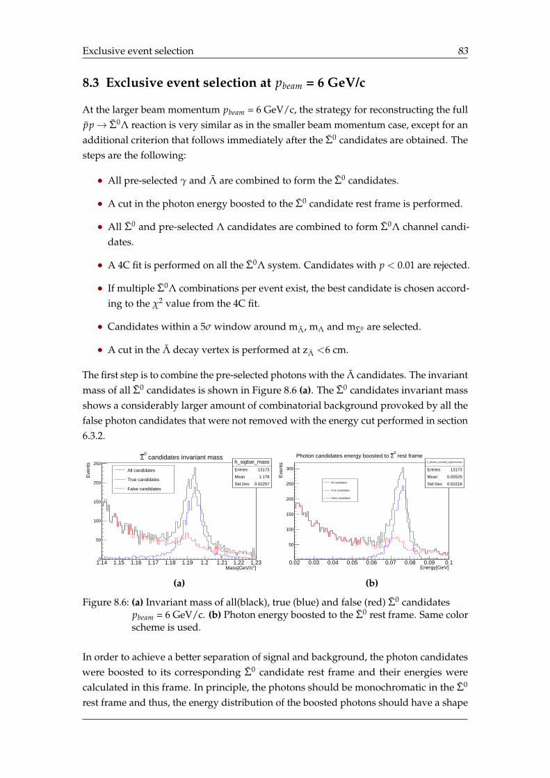
Exclusive event selection 83
8.3 Exclusive event selection at pbeam = 6 GeV/c
At the larger beam momentum pbeam = 6 GeV/c, the strategy for reconstructing the fullpp→ Σ0Λ reaction is very similar as in the smaller beam momentum case, except for anadditional criterion that follows immediately after the Σ0 candidates are obtained. Thesteps are the following:
• All pre-selected γ and Λ are combined to form the Σ0 candidates.
• A cut in the photon energy boosted to the Σ0 candidate rest frame is performed.
• All Σ0 and pre-selected Λ candidates are combined to form Σ0Λ channel candi-dates.
• A 4C fit is performed on all the Σ0Λ system. Candidates with p < 0.01 are rejected.
• If multiple Σ0Λ combinations per event exist, the best candidate is chosen accord-ing to the χ2 value from the 4C fit.
• Candidates within a 5σ window around mΛ, mΛ and mΣ0 are selected.
• A cut in the Λ decay vertex is performed at zΛ <6 cm.
The first step is to combine the pre-selected photons with the Λ candidates. The invariantmass of all Σ0 candidates is shown in Figure 8.6 (a). The Σ0 candidates invariant massshows a considerably larger amount of combinatorial background provoked by all thefalse photon candidates that were not removed with the energy cut performed in section6.3.2.
h_sigbar_massEntries 13173
Mean 1.178
Std Dev 0.02257
]2Mass[GeV/c1.14 1.15 1.16 1.17 1.18 1.19 1.2 1.21 1.22 1.23
Eve
nts
0
50
100
150
200
250 h_sigbar_massEntries 13173
Mean 1.178
Std Dev 0.02257
candidates invariant mass0
Σ
All candidates
True candidates
False candidates
(a)
h_photon_boosted_sigmissmass
Entries 13173
Mean 0.05529
Std Dev 0.02218
Energy[GeV]0.02 0.03 0.04 0.05 0.06 0.07 0.08 0.09 0.1
Eve
nts
50
100
150
200
250
300
h_photon_boosted_sigmissmass
Entries 13173
Mean 0.05529
Std Dev 0.02218
rest frame0
ΣPhoton candidates energy boosted to
All candidates
True candidates
False candidates
(b)
Figure 8.6: (a) Invariant mass of all(black), true (blue) and false (red) Σ0 candidatespbeam = 6 GeV/c. (b) Photon energy boosted to the Σ0 rest frame. Same colorscheme is used.
In order to achieve a better separation of signal and background, the photon candidateswere boosted to its corresponding Σ0 candidate rest frame and their energies werecalculated in this frame. In principle, the photons should be monochromatic in the Σ0
rest frame and thus, the energy distribution of the boosted photons should have a shape
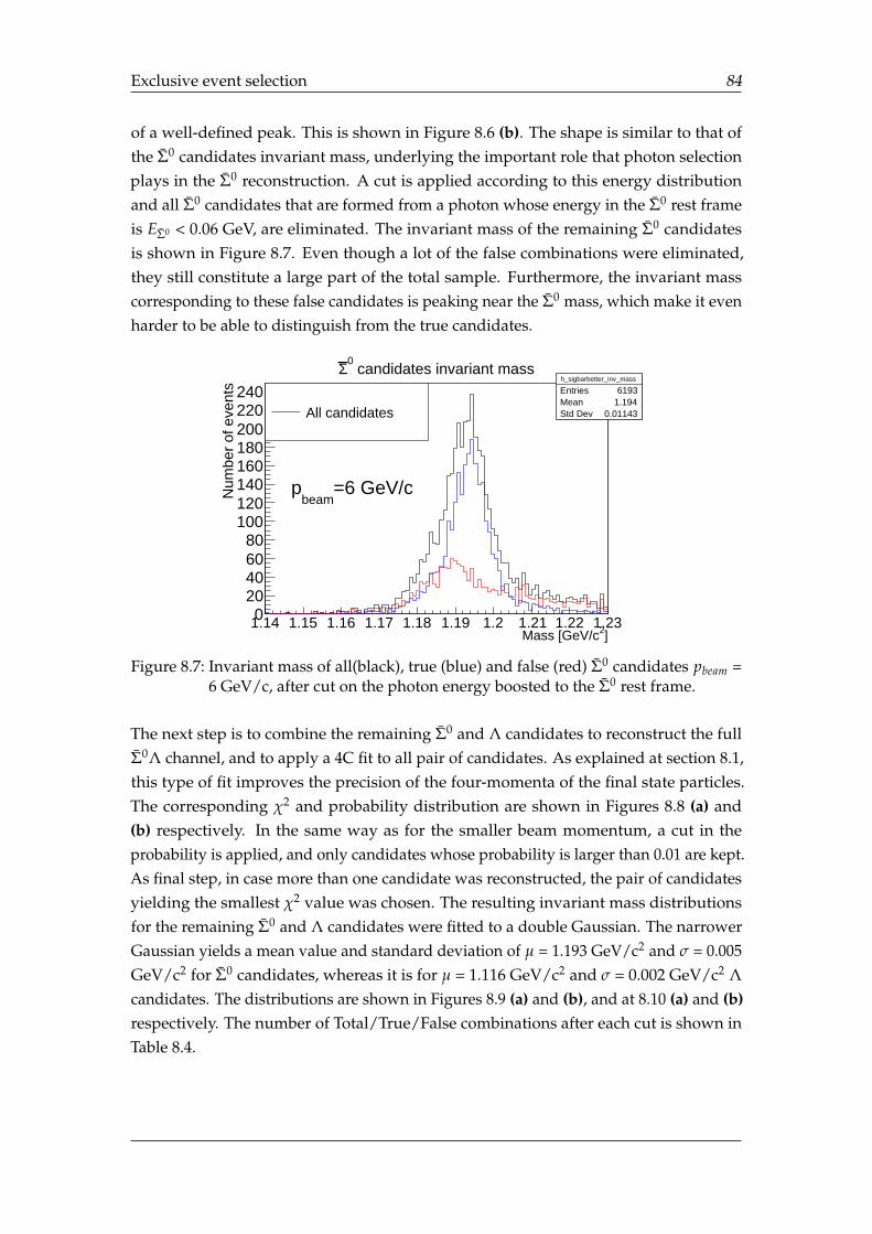
Exclusive event selection 84
of a well-defined peak. This is shown in Figure 8.6 (b). The shape is similar to that ofthe Σ0 candidates invariant mass, underlying the important role that photon selectionplays in the Σ0 reconstruction. A cut is applied according to this energy distributionand all Σ0 candidates that are formed from a photon whose energy in the Σ0 rest frameis EΣ0 < 0.06 GeV, are eliminated. The invariant mass of the remaining Σ0 candidatesis shown in Figure 8.7. Even though a lot of the false combinations were eliminated,they still constitute a large part of the total sample. Furthermore, the invariant masscorresponding to these false candidates is peaking near the Σ0 mass, which make it evenharder to be able to distinguish from the true candidates.
h_sigbarbetter_inv_mass
Entries 6193Mean 1.194Std Dev 0.01143
]2Mass [GeV/c1.14 1.15 1.16 1.17 1.18 1.19 1.2 1.21 1.22 1.23
Num
ber
of e
vent
s
020406080
100120140160180200220240
h_sigbarbetter_inv_mass
Entries 6193Mean 1.194Std Dev 0.01143All candidates
=6 GeV/cbeam
p
candidates invariant mass0Σ
Figure 8.7: Invariant mass of all(black), true (blue) and false (red) Σ0 candidates pbeam =6 GeV/c, after cut on the photon energy boosted to the Σ0 rest frame.
The next step is to combine the remaining Σ0 and Λ candidates to reconstruct the fullΣ0Λ channel, and to apply a 4C fit to all pair of candidates. As explained at section 8.1,this type of fit improves the precision of the four-momenta of the final state particles.The corresponding χ2 and probability distribution are shown in Figures 8.8 (a) and(b) respectively. In the same way as for the smaller beam momentum, a cut in theprobability is applied, and only candidates whose probability is larger than 0.01 are kept.As final step, in case more than one candidate was reconstructed, the pair of candidatesyielding the smallest χ2 value was chosen. The resulting invariant mass distributionsfor the remaining Σ0 and Λ candidates were fitted to a double Gaussian. The narrowerGaussian yields a mean value and standard deviation of µ = 1.193 GeV/c2 and σ = 0.005GeV/c2 for Σ0 candidates, whereas it is for µ = 1.116 GeV/c2 and σ = 0.002 GeV/c2 Λcandidates. The distributions are shown in Figures 8.9 (a) and (b), and at 8.10 (a) and (b)respectively. The number of Total/True/False combinations after each cut is shown inTable 8.4.
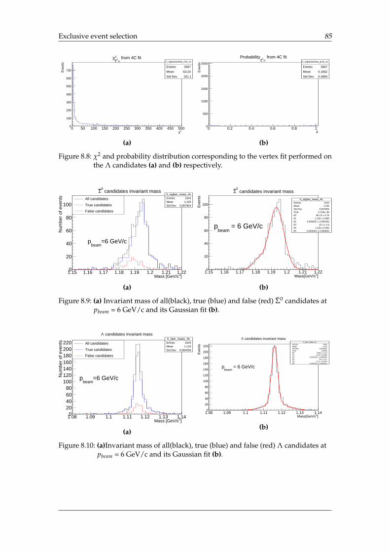
Exclusive event selection 85
h_sigbarlambda_chi2_4c
Entries 3567
Mean 63.24
Std Dev 101.1
2χ0 50 100 150 200 250 300 350 400 450 500
Eve
nts
0
100
200
300
400
500
600
700
h_sigbarlambda_chi2_4c
Entries 3567
Mean 63.24
Std Dev 101.1
from 4C fitΛ
0Σ
2χ
(a)
h_sigbarlambda_prob_4c
Entries 3567
Mean 0.1562
Std Dev 0.2894
p0 0.2 0.4 0.6 0.8 1
Eve
nts
0
500
1000
1500
2000
2500h_sigbarlambda_prob_4c
Entries 3567
Mean 0.1562
Std Dev 0.2894
from 4C fitΛ
0Σ
Probability
(b)
Figure 8.8: χ2 and probability distribution corresponding to the vertex fit performed onthe Λ candidates (a) and (b) respectively.
h_sigbar_mass_4cEntries 1043Mean 1.193Std Dev 0.007804
]2Mass [GeV/c1.15 1.16 1.17 1.18 1.19 1.2 1.21 1.22
Num
ber
of e
vent
s
0
20
40
60
80
100
h_sigbar_mass_4cEntries 1043Mean 1.193Std Dev 0.007804
All candidates
True candidates
False candidates
=6 GeV/cbeam
p
candidates invariant mass0Σ
(a)
h_sigbar_mass_4cEntries 1043Mean 1.193Std Dev 0.007804Prob 06− 5.154ep0 4.76± 95.13 p1 0.000± 1.193 p2 0.000302± 0.004822 p3 3.4± 13.1 p4 0.002± 1.181 p5 0.000853± 0.003434
]2Mass[GeV/c1.15 1.16 1.17 1.18 1.19 1.2 1.21 1.22
Eve
nts
0
20
40
60
80
100
h_sigbar_mass_4cEntries 1043Mean 1.193Std Dev 0.007804Prob 06− 5.154ep0 4.76± 95.13 p1 0.000± 1.193 p2 0.000302± 0.004822 p3 3.4± 13.1 p4 0.002± 1.181 p5 0.000853± 0.003434
candidates invariant mass0
Σ
= 6 GeV/cbeam
p
(b)
Figure 8.9: (a) Invariant mass of all(black), true (blue) and false (red) Σ0 candidates atpbeam = 6 GeV/c and its Gaussian fit (b).
h_lam_mass_4cEntries 1043Mean 1.116Std Dev 0.004256
]2Mass [GeV/c1.08 1.09 1.1 1.11 1.12 1.13 1.14
Num
ber
of e
vent
s
020406080
100120140160180200220
h_lam_mass_4cEntries 1043Mean 1.116Std Dev 0.004256
All candidates
True candidates
False candidates
=6 GeV/cbeam
p
candidates invariant massΛ
(a)
h_lam_mass_4cEntries 1043Mean 1.116Std Dev 0.004256Prob 0.6458p0 11.0± 199.3 p1 0.000± 1.116 p2 0.000090± 0.001632 p3 4.2± 24.1 p4 0.000± 1.117 p5 0.000513± 0.006313
]2Mass[GeV/c1.08 1.09 1.1 1.11 1.12 1.13 1.14
Eve
nts
0
20
40
60
80
100
120
140
160
180
200
220h_lam_mass_4c
Entries 1043Mean 1.116Std Dev 0.004256Prob 0.6458p0 11.0± 199.3 p1 0.000± 1.116 p2 0.000090± 0.001632 p3 4.2± 24.1 p4 0.000± 1.117 p5 0.000513± 0.006313
candidates invariant massΛ
= 6 GeV/cbeam
p
(b)
Figure 8.10: (a)Invariant mass of all(black), true (blue) and false (red) Λ candidates atpbeam = 6 GeV/c and its Gaussian fit (b).
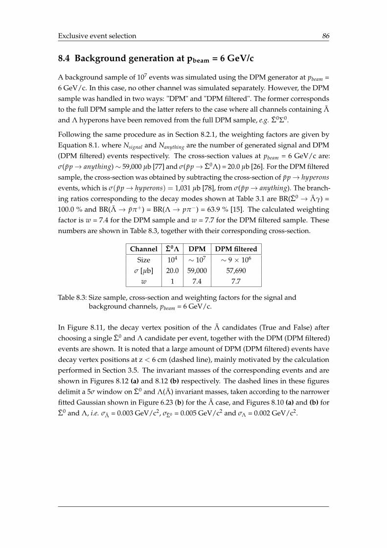
Exclusive event selection 86
8.4 Background generation at pbeam = 6 GeV/c
A background sample of 107 events was simulated using the DPM generator at pbeam =6 GeV/c. In this case, no other channel was simulated separately. However, the DPMsample was handled in two ways: "DPM" and "DPM filtered". The former correspondsto the full DPM sample and the latter refers to the case where all channels containing Λand Λ hyperons have been removed from the full DPM sample, e.g. Σ0Σ0.
Following the same procedure as in Section 8.2.1, the weighting factors are given byEquation 8.1. where Nsignal and Nanything are the number of generated signal and DPM(DPM filtered) events respectively. The cross-section values at pbeam = 6 GeV/c are:σ(pp→ anything)∼ 59,000 µb [77] and σ(pp→ Σ0Λ) = 20.0 µb [26]. For the DPM filteredsample, the cross-section was obtained by subtracting the cross-section of pp→ hyperonsevents, which is σ( pp→ hyperons) = 1,031 µb [78], from σ(pp→ anything). The branch-ing ratios corresponding to the decay modes shown at Table 3.1 are BR(Σ0 → Λγ) =100.0 % and BR(Λ → pπ+) = BR(Λ → pπ−) = 63.9 % [15]. The calculated weightingfactor is w = 7.4 for the DPM sample and w = 7.7 for the DPM filtered sample. Thesenumbers are shown in Table 8.3, together with their corresponding cross-section.
Channel Σ0Λ DPM DPM filteredSize 104 ∼ 107 ∼ 9 × 10⁶
σ [µb] 20.0 59,000 57,690w 1 7.4 7.7
Table 8.3: Size sample, cross-section and weighting factors for the signal andbackground channels, pbeam = 6 GeV/c.
In Figure 8.11, the decay vertex position of the Λ candidates (True and False) afterchoosing a single Σ0 and Λ candidate per event, together with the DPM (DPM filtered)events are shown. It is noted that a large amount of DPM (DPM filtered) events havedecay vertex positions at z < 6 cm (dashed line), mainly motivated by the calculationperformed in Section 3.5. The invariant masses of the corresponding events and areshown in Figures 8.12 (a) and 8.12 (b) respectively. The dashed lines in these figuresdelimit a 5σ window on Σ0 and Λ(Λ) invariant masses, taken according to the narrowerfitted Gaussian shown in Figure 6.23 (b) for the Λ case, and Figures 8.10 (a) and (b) forΣ0 and Λ, i.e. σΛ = 0.003 GeV/c2, σΣ0 = 0.005 GeV/c2 and σΛ = 0.002 GeV/c2.
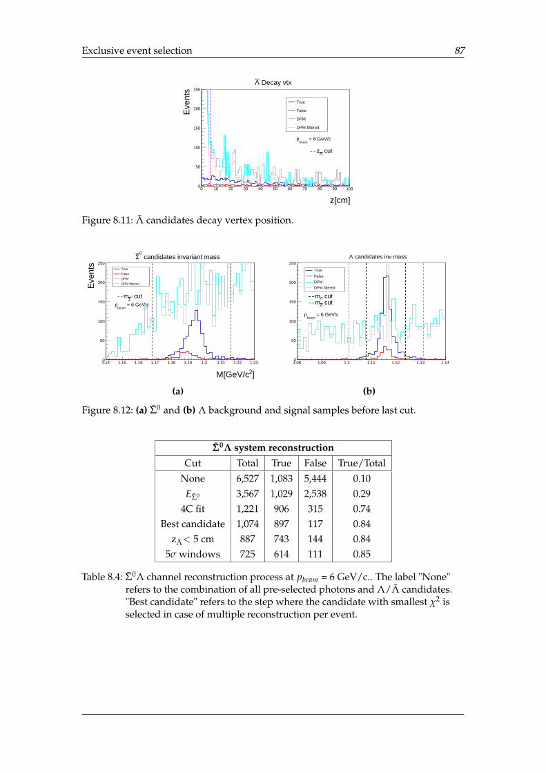
Exclusive event selection 87
z[cm]
0 10 20 30 40 50 60 70 80 90 100E
vent
s0
50
100
150
200
250
= 6 GeV/cbeam
p
True
False
DPM
DPM filtered
cutΛz
Decay vtxΛ
Figure 8.11: Λ candidates decay vertex position.
]2M[GeV/c
1.14 1.15 1.16 1.17 1.18 1.19 1.2 1.21 1.22 1.23
Eve
nts
0
50
100
150
200
250
= 6 GeV/cbeam
p
True
False
DPM
DPM filtered
cut0Σ
m
candidates invariant mass0
Σ
(a)
1.08 1.09 1.1 1.11 1.12 1.13 1.140
50
100
150
200
250
= 6 GeV/cbeam
p
True
False
DPM
DPM filtered
cutΛm cutΛm
candidates inv massΛ
(b)
Figure 8.12: (a) Σ0 and (b) Λ background and signal samples before last cut.
Σ0Λ system reconstructionCut Total True False True/Total
None 6,527 1,083 5,444 0.10EΣ0 3,567 1,029 2,538 0.29
4C fit 1,221 906 315 0.74Best candidate 1,074 897 117 0.84
zΛ< 5 cm 887 743 144 0.845σ windows 725 614 111 0.85
Table 8.4: Σ0Λ channel reconstruction process at pbeam = 6 GeV/c.. The label "None"refers to the combination of all pre-selected photons and Λ/Λ candidates."Best candidate" refers to the step where the candidate with smallest χ2 isselected in case of multiple reconstruction per event.
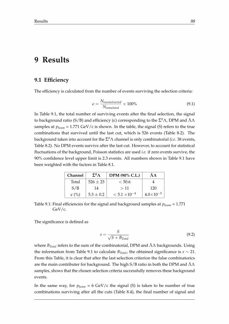
Results 88
9 Results
9.1 Efficiency
The efficiency is calculated from the number of events surviving the selection criteria:
ε =Nreconstructed
Nsimulated× 100% (9.1)
In Table 9.1, the total number of surviving events after the final selection, the signalto background ratio (S/B) and efficiency (ε) corresponding to the Σ0Λ, DPM and ΛΛsamples at pbeam = 1.771 GeV/c is shown. In the table, the signal (S) refers to the truecombinations that survived until the last cut, which is 526 events (Table 8.2). Thebackground taken into account for the Σ0Λ channel is only combinatorial (i.e. 38 events,Table 8.2). No DPM events survive after the last cut. However, to account for statisticalfluctuations of the background, Poisson statistics are used i.e. if zero events survive, the90% confidence level upper limit is 2.3 events. All numbers shown in Table 9.1 havebeen weighted with the factors in Table 8.1.
Channel Σ0Λ DPM (90% C.L.) ΛΛ
Total 526 ± 23 < 50.6 4S/B 14 > 11 120ε (%) 5.3 ± 0.2 < 5.1 ×10⁻⁴ 4.0×10⁻⁵
Table 9.1: Final efficiencies for the signal and background samples at pbeam = 1.771GeV/c.
The significance is defined as
s =S√
S + BTotal(9.2)
where BTotal refers to the sum of the combinatorial, DPM and ΛΛ backgrounds. Usingthe information from Table 9.1 to calculate BTotal , the obtained significance is s ∼ 21.From this Table, it is clear that after the last selection criterion the false combinatoricsare the main contributer for background. The high S/B ratio in both the DPM and ΛΛsamples, shows that the chosen selection criteria successfully removes these backgroundevents.
In the same way, for pbeam = 6 GeV/c the signal (S) is taken to be number of truecombinations surviving after all the cuts (Table 8.4), the final number of signal and
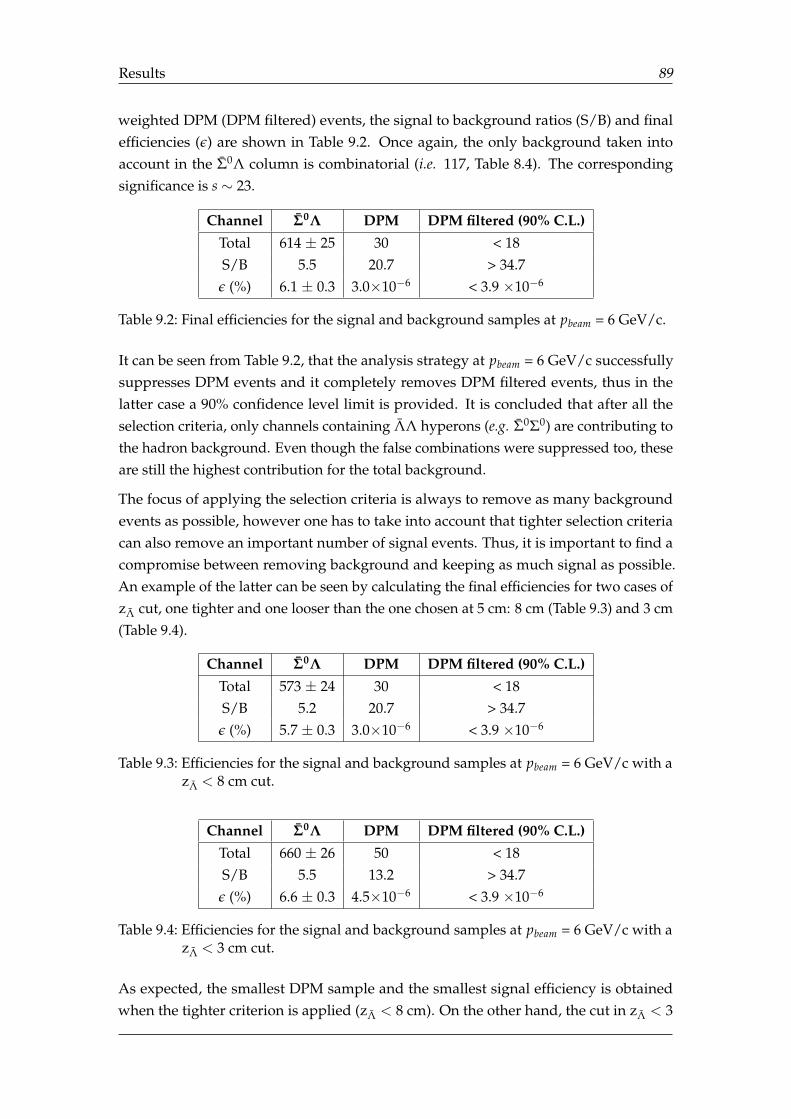
Results 89
weighted DPM (DPM filtered) events, the signal to background ratios (S/B) and finalefficiencies (ε) are shown in Table 9.2. Once again, the only background taken intoaccount in the Σ0Λ column is combinatorial (i.e. 117, Table 8.4). The correspondingsignificance is s ∼ 23.
Channel Σ0Λ DPM DPM filtered (90% C.L.)Total 614 ± 25 30 < 18S/B 5.5 20.7 > 34.7ε (%) 6.1 ± 0.3 3.0×10⁻⁶ < 3.9 ×10⁻⁶
Table 9.2: Final efficiencies for the signal and background samples at pbeam = 6 GeV/c.
It can be seen from Table 9.2, that the analysis strategy at pbeam = 6 GeV/c successfullysuppresses DPM events and it completely removes DPM filtered events, thus in thelatter case a 90% confidence level limit is provided. It is concluded that after all theselection criteria, only channels containing ΛΛ hyperons (e.g. Σ0Σ0) are contributing tothe hadron background. Even though the false combinations were suppressed too, theseare still the highest contribution for the total background.
The focus of applying the selection criteria is always to remove as many backgroundevents as possible, however one has to take into account that tighter selection criteriacan also remove an important number of signal events. Thus, it is important to find acompromise between removing background and keeping as much signal as possible.An example of the latter can be seen by calculating the final efficiencies for two cases ofzΛ cut, one tighter and one looser than the one chosen at 5 cm: 8 cm (Table 9.3) and 3 cm(Table 9.4).
Channel Σ0Λ DPM DPM filtered (90% C.L.)Total 573 ± 24 30 < 18S/B 5.2 20.7 > 34.7ε (%) 5.7 ± 0.3 3.0×10⁻⁶ < 3.9 ×10⁻⁶
Table 9.3: Efficiencies for the signal and background samples at pbeam = 6 GeV/c with azΛ < 8 cm cut.
Channel Σ0Λ DPM DPM filtered (90% C.L.)Total 660 ± 26 50 < 18S/B 5.5 13.2 > 34.7ε (%) 6.6 ± 0.3 4.5×10⁻⁶ < 3.9 ×10⁻⁶
Table 9.4: Efficiencies for the signal and background samples at pbeam = 6 GeV/c with azΛ < 3 cm cut.
As expected, the smallest DPM sample and the smallest signal efficiency is obtainedwhen the tighter criterion is applied (zΛ < 8 cm). On the other hand, the cut in zΛ < 3
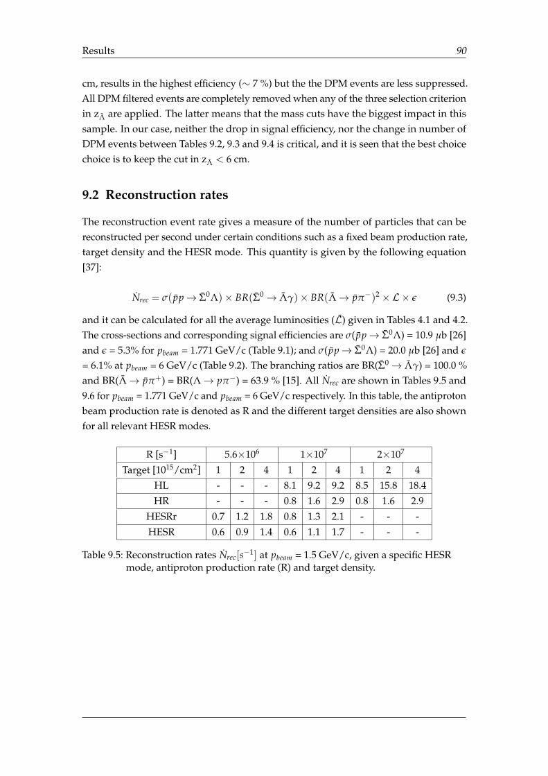
Results 90
cm, results in the highest efficiency (∼ 7 %) but the the DPM events are less suppressed.All DPM filtered events are completely removed when any of the three selection criterionin zΛ are applied. The latter means that the mass cuts have the biggest impact in thissample. In our case, neither the drop in signal efficiency, nor the change in number ofDPM events between Tables 9.2, 9.3 and 9.4 is critical, and it is seen that the best choicechoice is to keep the cut in zΛ < 6 cm.
9.2 Reconstruction rates
The reconstruction event rate gives a measure of the number of particles that can bereconstructed per second under certain conditions such as a fixed beam production rate,target density and the HESR mode. This quantity is given by the following equation[37]:
Nrec = σ( pp→ Σ0Λ)× BR(Σ0→ Λγ)× BR(Λ→ pπ−)2 ×L× ε (9.3)
and it can be calculated for all the average luminosities (L) given in Tables 4.1 and 4.2.The cross-sections and corresponding signal efficiencies are σ(pp→ Σ0Λ) = 10.9 µb [26]and ε = 5.3% for pbeam = 1.771 GeV/c (Table 9.1); and σ(pp→ Σ0Λ) = 20.0 µb [26] and ε
= 6.1% at pbeam = 6 GeV/c (Table 9.2). The branching ratios are BR(Σ0→ Λγ) = 100.0 %and BR(Λ→ pπ+) = BR(Λ→ pπ−) = 63.9 % [15]. All Nrec are shown in Tables 9.5 and9.6 for pbeam = 1.771 GeV/c and pbeam = 6 GeV/c respectively. In this table, the antiprotonbeam production rate is denoted as R and the different target densities are also shownfor all relevant HESR modes.
R [s−1] 5.6×10⁶ 1×10⁷ 2×10⁷
Target [1015/cm2] 1 2 4 1 2 4 1 2 4
HL - - - 8.1 9.2 9.2 8.5 15.8 18.4
HR - - - 0.8 1.6 2.9 0.8 1.6 2.9
HESRr 0.7 1.2 1.8 0.8 1.3 2.1 - - -
HESR 0.6 0.9 1.4 0.6 1.1 1.7 - - -
Table 9.5: Reconstruction rates Nrec[s−1] at pbeam = 1.5 GeV/c, given a specific HESRmode, antiproton production rate (R) and target density.
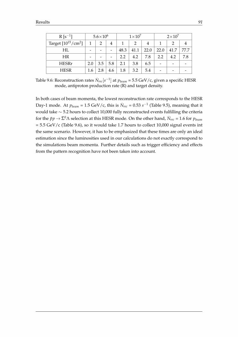
Results 91
R [s−1] 5.6×10⁶ 1×10⁷ 2×10⁷
Target [1015/cm2] 1 2 4 1 2 4 1 2 4
HL - - - 48.3 41.1 22.0 22.0 41.7 77.7
HR - - - 2.2 4.2 7.8 2.2 4.2 7.8
HESRr 2.0 3.5 5.8 2.1 3.8 6.5 - - -
HESR 1.6 2.8 4.6 1.8 3.2 5.4 - - -
Table 9.6: Reconstruction rates Nrec[s−1] at pbeam = 5.5 GeV/c, given a specific HESRmode, antiproton production rate (R) and target density.
In both cases of beam momenta, the lowest reconstruction rate corresponds to the HESRDay-1 mode. At pbeam = 1.5 GeV/c, this is Nrec = 0.53 s−1 (Table 9.5), meaning that itwould take ∼ 5.2 hours to collect 10,000 fully reconstructed events fulfilling the criteriafor the pp→ Σ0Λ selection at this HESR mode. On the other hand, Nrec = 1.6 for pbeam
= 5.5 GeV/c (Table 9.6), so it would take 1.7 hours to collect 10,000 signal events intthe same scenario. However, it has to be emphasized that these times are only an idealestimation since the luminosities used in our calculations do not exactly correspond tothe simulations beam momenta. Further details such as trigger efficiency and effectsfrom the pattern recognition have not been taken into account.
Summary and Conclusions 92
10 Summary and Conclusions
A simulation study of the feasibility for reconstructing the pp→ Σ0Λ reaction with thePANDA experiment has been performed. Two samples of 104 events were simulated:one at beam momentum pbeam = 1.771 GeV/c and one at pbeam = 6 GeV/c. Both sampleswere generated using an angular distribution parametrization based on experimentaldata. At the smaller beam momentum, an inclusive and an exclusive event selectionwere performed, whereas for the higher beam momentum, only exclusive event selectionwas carried out.
The photon selection proved to be one of the most crucial steps. In both cases, secondaryphotons contaminate the signal. Therefore, eliminating false photon candidates is ofuttermost importance to achieve a clean sample. It was concluded that the standardway PandaRoot defines photons, might cause misidentification of other neutral or evencharged particles as photons. Kinematic cuts on the photons reduced the amount offalse photons with a factor of 12 in the case of pbeam = 1.771 GeV/c and by a factor of 6 inthe case of pbeam = 6 GeV/c.
From the inclusive event selection performed at pbeam = 1.771 GeV/c, in which thereaction of the form pp→ Σ0X was reconstructed, the distinction between signal andcombinatorial background was very difficult, since the variable that is used for identi-fication, i.e. the γ pπ+ invariant mass has a peaking background distribution at the Σ0
mass. The conclusion is that partial channel reconstruction is not feasible for pursuingthe clean samples required for spin observable extraction.
On the other hand, the selection criteria used for the exclusive event selection at pbeam =1.771 GeV/c, provides with a sample reasonably clean from combinatorial background.Moreover, two background samples were simulated at this beam momentum: one givenby the Dual Parton Model generator and one of the pp→ ΛΛ reaction only. The selectionprocess also proved to be efficient by completely removing the DPM background events.Therefore, only Poisson upper limits of the background level has been calculated. Thefinal efficiency was ε = 5.3% ± 0.2%, S/BTotal ∼6 and significance ∼21 for the Σ0Λchannel at this beam momentum.
In the case of the pbeam = 6 GeV/c sample, the reconstruction strategy required for atighter photon selection. This proved to be successful in suppressing DPM events andno other channel was independently generated. However, the fact that all the "DPMfiltered" events were removed, highlights the importance of testing the analysis strategywith independent samples of channels containing ΛΛ events (e.g. pp→ Σ0Σ0). The final
Summary and Conclusions 93
signal efficiency for pp→ Σ0Λ events was ε = 6.1%± 0.3%, S/BTotal ∼ 4 and significance∼22.
The efficiencies obtained for pbeam = 1.771 GeV/c and pbeam = 6 GeV/c are both smallerthan the one obtained in the previous simulation study (Ref [43]), by a factor of 6 and4, respectively. It should be pointed out though, that the previous study the usedmomentum was pbeam = 4 GeV/c, it is nevertheless a value in-between the beam mo-menta used in this work and therefore, it is reasonably to think that the correspondingefficiency would be of the same order of magnitude as the ones obtained here. Thedrop in efficiency compared to the previous study to this updated study underlines theimportance on using a realistic angular momentum distribution and the correct detectorimplementation. Nevertheless, the result shows that it is feasible to study exclusivepp→ Σ0Λ production in PANDA. With the Day-1 luminosity (Tables 4.1 and Table 4.2)and the obtained efficiencies, it would take ∼ 5.2 hours and ∼ 1.7 hours to collect 10,000signal events for pbeam = 1.771 GeV/c and pbeam = 6 Gev/c, respectiely.
Literature 94
Literature
[1] M.K. Gaillard et al., The Standard model of particle physics, Rev. Mod. Phys. 71 (1999)S96
[2] Git-Hub repository: https://github.com/mlubej/standard-model
[3] N. Cabibbo, Unitary Symmetry and Leptonic Decays, Phys. Rev. Lett. 10 (1963) 531.
[4] M. Kobayashi and T. Maskawa, CP Violation in the Renormalizable Theory of WeakInteraction, Prog. Theor. Phys. 49 (1973) 652.
[5] K. Huang, Fundamental forces of nature: The story of gauge fields Hackensack, USA:World Scientific (2007) 270 p
[6] H. Fritzsch et al., Advantages of the Color Octet Gluon Picture, Phys. Lett. 47B (1973)365.
[7] H. D. Politzer, Reliable Perturbative Results for Strong Interactions?, Phys. Rev. Lett. 30(1973) 1346.
[8] D. J. Gross and F. Wilczek, Ultraviolet Behavior of Nonabelian Gauge Theories, Phys. Rev.Lett. 30 (1973) 1343.
[9] F. Englert and R. Brout, Broken Symmetry and the Mass of Gauge Vector Mesons, Phys.Rev. Lett. 13 (1964) 321.
[10] P. W. Higgs, Broken Symmetries and the Masses of Gauge Bosons, Phys. Rev. Lett. 13(1964) 508.
[11] G. Aad et al. [ATLAS Collaboration], Observation of a new particle in the search for theStandard Model Higgs boson with the ATLAS detector at the LHC, Phys. Lett. B 716 (2012)1
[12] J. H. Christenson et al., Evidence for the 2π Decay of the K02 Meson, Phys. Rev. Lett. 13
(1964) 138.
[13] B. Kayser, Are neutrinos their own antiparticles?, J. Phys. Conf. Ser. 173 (2009) 012013
[14] R. Aaij et al. [LHCb Collaboration], Measurement of matter-antimatter differences inbeauty baryon decays, Nature Phys. 13 (2017) 391
[15] M. Tanabashi et al. [Particle Data Group], Review of Particle Physics, Phys. Rev. D 98(2018) no.3, 030001.
Literature 95
[16] S. Godfrey and N. Isgur, Mesons in a Relativized Quark Model with Chromodynamics,Phys. Rev. D 32 (1985) 189.
[17] C. A. Aidala et al., The Spin Structure of the Nucleon, Rev. Mod. Phys. 85 (2013) 655
[18] S. Scherer, and M. R. Schindler, Quantum chromodynamics and chiral symmetry. In APrimer for Chiral Perturbation Theory, Springer, Berlin, Heidelberg. (2011) 1-48.
[19] R. Pohl, et al., The size of the proton, Nature, 466(7303), (2010) 213.
[20] L. G. Landsberg, The search for exotic hadrons, Phys. Usp. 42 (1999) 871
[21] E. Thomé, Multi-Strange and Charmed Antihyperon-Hyperon Physics for PANDA, TH-PHD-2012-001.
[22] M. Ablikim et al. [BESIII Collaboration], Observation of a Charged CharmoniumlikeStructure in e+e−→ π+π− J/ψ at
√s = 4.26 GeV, Phys. Rev. Lett. 110 (2013) 252001
[23] Z. Q. Liu et al. [Belle Collaboration], Study of e+e−→ π+π−J/ψ and Observation ofa Charged Charmoniumlike State at Belle Phys. Rev. Lett. 110 (2013) 252002
[24] R. Aaij et al. [LHCb Collaboration], Observation of J/ψp Resonances Consisten withPentaquark States in Λ0
b→ J/ψ Decays Phys. Rev. Lett. 115 (2015) 072001
[25] Sakurai, J. J., & Commins, E. D., Modern quantum mechanics, revised edition. (1995).
[26] P. D. Barnes et al., Measurement of the anti-p p —> anti-lambda Lambda and anti-p p—> Antisigma0 Lambda + c.c. reactions at 1.726-GeV/c and 1.771-GeV/c, Phys. Rev. C 54(1996) 2831.
[27] Johansson T, AIP Conf. Proc. 8th Int. Conf. on Low Energy Antiproton Physics, 95 (2003)
[28] F. Tabakin and R. A. Eisenstein, Meson Exchange Calculation of the pp→ ΛΛ Reaction,Phys. Rev. C 31 (1985) 1857.
[29] A. M. Green and J. A. Niskanen, Low-energy Anti-proton Physics in the Early LEAREra, Prog. Part. Nucl. Phys. 18 (1987) 93.
[30] M. Kohno and W. Weise, The anti-p p —> anti-Lambda Lambda Reaction Close toThreshold, Phys. Lett. B 206 (1988) 584.
[31] Weise, W., Antinucleon-nucleon annihilation. Nuclear Physics A 558, (1993), 219-233.
[32] P. LaFrance and B. Loiseau, Study from threshold to high momenta of the anti-p p —>anti-Lambda Lambda reaction, Nucl. Phys. A 528 (1991) 557.
[33] Lu, Y., and M. P. Locher. Regge pole model with K ∗ −K ∗ ∗ exchange and absorption forthe ΛΛ reaction. Zeitschrift für Physik A Hadrons and Nuclei 346(2) (1993), 143-151.
Literature 96
[34] J. Haidenbauer et al., The Reaction anti-p p —> anti-Lambda Lambda in the mesonexchange picture, Phys. Rev. C 45 (1992) 931.
[35] J. Haidenbauer et al., Anti-hyperon - hyperon production in the meson exchange frame-work, Phys. Rev. C 46 (1992) 2516.
[36] J. Haidenbauer et al., Meson exchange and quark - gluon transitions in the anti-p p —>anti-Lambda Lambda process, Phys. Rev. C 46 (1992) 2158.
[37] I. Andersson, W., Measurement of Spin Observables in the pp→ ΛΛ reaction at PANDARN-NOP-2018-003 (2018)
[38] P. D. Barnes et al., Measurement of the Reaction pp→ ¯ambda Sigma0 + c.c. At 1.695-GeV/c, Phys. Lett. B 246 (1990) 273.
[39] Tayloe, R. L., A measurement of the pp→ ΛΛ and pp→ Σ0Λ + c.c. reactions at 1.726GeV/c, University of Illinois at Urbana-Champaign, (1995)
[40] H. Becker et al. [CERN-Munich Collaboration], Measurement of the Reactions PP→ΛΛ, pp→ ΛΣ0 and PP→ Λ (Missing Mass) at 6-GeV, Nucl. Phys. B 141 (1978) 48.
[41] G. Plaut, Exchange-degeneracy and absorption in anti-p p —> anti-y y, Nucl. Phys. B 35(1971) 221.
[42] B. Sadoulet, Phenomenological characteristics of absorption in charge- and hypercharge-exchange reactions, Nucl. Phys. B 53 (1973) 135.
[43] Grape, S., Studies of PWO Crystals and Simulations of the pp→ ΛΛ, ΛΣ0 Reactions forthe PANDA Experiment. PhD thesis, Uppsala University (2009).
[44] Hamel de Monchenault, G., The BaBar Computing Model. Stanford Linear AcceleratorCenter, Menlo Park, CA (US), No. SLAC-PUB-9964 (2003).
[45] FAIR webpage, https://fair-center.eu/
[46] M. F. M. Lutz et al. [PANDA Collaboration], Physics Performance Report for PANDA:Strong Interaction Studies with Antiprotons,
[47] W. Erni et al [PANDA Collaboration], Technical Design Report for the PANDA InternalTargets: The Cluster-Jet Target and Developments for the Pellet Target. (2012).
[48] Götzen K., Average Luminosities and Event Rates at PANDA IN-IDE-2015-002 (2018)
[49] PANDA webpage, https://panda.gsi.de/
[50] W. Erni et al [PANDA Collaboration], Technical Design Report for the: PANDA MicroVertex Detector. (2012)
[51] W. Erni et al. [PANDA Collaboration], Technical design report for the PANDA (AntiPro-ton Annihilations at Darmstadt) Straw Tube Tracker, Eur. Phys. J. A 49 (2013) 25

Literature 97
[52] B. Singh et al. [PANDA Collaboration], Technical Design Report for the PANDA BarrelDIRC Detector,
[53] PANDA Collaboration. Technical Design Report for the: PANDA Barrel Time-of-Flight(2018)
[54] W. Erni et al. [PANDA Collaboration], Technical Design Report for PANDA Electro-magnetic Calorimeter (EMC),
[55] W. Erni et al. [PANDA Collaboration], Technical Design Report for the PANDA MuonSystem (2012)
[56] J. Smyrski et al. [PANDA Collaboration], Design of the forward straw tube tracker forthe PANDA experiment, JINST 12 (2017) no.06, C06032.
[57] W. Erni et al. [PANDA Collaboration], Forward Time of Flight detector (FToF wall)(2018)
[58] W. Erni et al. [PANDA Collaboration], Technical Design Report for the Panda ForwardSpectrometer Calorimeter,
[59] Wavelength shifter definition: https://en.wikipedia.org/wiki/Wavelength_shifterWikipedia
[60] M. Sudol et al., Feasibility studies of the time-like proton electromagnetic form factormeasurements with PANDA at FAIR, Eur. Phys. J. A 44 (2010) 373
[61] A. Freund et al., Exclusive annihilation p anti-p —> gamma gamma in a generalizedparton picture, Phys. Rev. Lett. 90 (2003) 092001
[62] L. L. Frankfurt et al., Hard exclusive pseudoscalar meson electroproduction and spinstructure of a nucleon, Phys. Rev. D 60 (1999) 014010
[63] B. Pire and L. Szymanowski, Hadron annihilation into two photons and backward VCSin the scaling regime of QCD, Phys. Rev. D 71 (2005) 111501
[64] R. Chistov, Study of charmonium(-like) states at BaBar and Belle,
[65] S. Spataro [PANDA Collaboration], The PandaRoot framework for simulation, recon-struction and analysis, J. Phys. Conf. Ser. 331 (2011) 032031.
[66] Brun, R. et al, ROOT-an object oriented data analysis framework. Nuclear Instrumentsand Methods in Physics Research Section A: Accelerators, Spectrometers, Detectorsand Associated Equipment 389(1-2), (1997), 81-86
[67] Stockmanns, T., Introduction PANDA Computing School 2017 - SUT Presentation,https://indico.gsi.de/event/4894/contribution/1/material/slides/1.pdf(2017)
Literature 98
[68] Spataro, S., EvtGen inside PandaRooT Presentation, https://panda.gsi.de/oldwww/html/com/frm/meeting/spataro_251006.pdf
[69] M. Asai, Geant4-a simulation toolkit, Trans. Amer. Nucl. Soc. 95 (2006) 757.
[70] Virtual Monte Carlo, https://root.cern.ch/root/vmc/
[71] S. Spataro [PANDA Collaboration], Simulation and event reconstruction inside thePandaRoot framework, J. Phys. Conf. Ser. 119 (2008) 032035.
[72] D. Brown et al. The babar track fitting algorithm, proc. computing in high energy physicsconference. Proc. Computing in High Energy Physics Conference, Padova. (2000).
[73] R. Fruehwirth and S. Fruehwirth-Schnatter, On the treatment of energy loss in trackfitting, Comput. Phys. Commun. 110 (1998) 80.
[74] S. Spataro, Event Reconstruction in the PandaRoot framework. Journal of Physics:Conference Series. Vol. 396. No. 2. IOP Publishing, (2012).
[75] P. Avery, Applied Fitting Theory VI: Formulas for Kinematic Fitting. CBX (1999) 98-37
[76] K. Götzen, pp Cross-section estimator https://panda.gsi.de/pbarx/index.php?&mode=1 (2014)
[77] V. Flaminio et al., Compilation of cross-sections: p and p bar induced reactions (1984)CERN/HERA 84-01
[78] C. Y. Chien Hyperon and anti-hyperon production in anti-p p collisions at 7 BeV/c, Phys.Rev. 152 (1966) 1171.