PRODUCTION AND DISTRIBUTION PLANNING FOR...

PRODUCTION AND DISTRIBUTION PLANNINGFOR DYNAMIC SUPPLY CHAINS USINGMULTI-RESOLUTION HYBRID MODELS

Item Type text; Electronic Dissertation

Authors Venkateswaran, Jayendran

Publisher The University of Arizona.

Rights Copyright © is held by the author. Digital access to this materialis made possible by the University Libraries, University of Arizona.Further transmission, reproduction or presentation (such aspublic display or performance) of protected items is prohibitedexcept with permission of the author.

Download date 18/06/2018 16:15:12

Link to Item http://hdl.handle.net/10150/195051

http://hdl.handle.net/10150/195051

PRODUCTION AND DISTRIBUTION PLANNING FOR DYNAMIC

SUPPLY CHAINS USING MULTI-RESOLUTION HYBRID MODELS

By

Jayendran Venkateswaran

A Dissertation Submitted to the Faculty of the

DEPARTMENT OF SYSTEMS AND INDUSTRIAL ENGINEERING

In Partial Fulfillment of the Requirements for the Degree of

DOCTOR OF PHILOSOPHY

In the Graduate College

THE UNIVERSITY OF ARIZONA

2 0 0 5

2

THE UNIVERSITY OF ARIZONA

GRADUATE COLLEGE

As members of the Dissertation Committee, we certify that we have read the dissertation

prepared by Jayendran Venkateswaran

entitled “Production and Distribution Planning in Dynamic Supply Chains using Multi-

Resolution Hybrid Models,”

and recommend that it be accepted as fulfilling the dissertation requirement for the

degree of Doctor of Philosophy.

_______________________________________________________________________ Date: May 10 2005

Young-Jun Son _______________________________________________________________________ Date: May 10 2005

Ronald G. Askin _______________________________________________________________________ Date May 10 2005

Jeffery B. Goldberg _______________________________________________________________________ Date: May 10 2005

Terry A. Bahill _______________________________________________________________________ Date: May 10 2005

Timothy W. Secomb Final approval and acceptance of this dissertation is contingent upon the candidate’s submission of the final copies of the dissertation to the Graduate College. I hereby certify that I have read this dissertation prepared under my direction and recommend that it be accepted as fulfilling the dissertation requirement. ________________________________________________ Date: May 10 2005 Dissertation Director: Young-Jun Son

3

STATEMENT BY AUTHOR

This dissertation has been submitted in partial fulfillment of requirements for an advanced degree at The University of Arizona and is deposited in the University Library to be made available to borrowers under rules of the Library.

Brief quotations from this dissertation are allowable without special permission, provided that accurate acknowledgment of source is made. Requests for permission for extended quotation from or reproduction of this manuscript in whole or in part may be granted by the head of the major department or the Dean of the Graduate College when in his or her judgment the proposed use of the material is in the interests of scholarship. In all other instances, however, permission must be obtained from the author.

SIGNED: ______________________________ Jayendran Venkateswaran

4

ACKNOWLEDGEMENTS

This dissertation would not have been possible without the guidance of my professors, support of my friends and the love of my family. I express my sincere thanks to those who made my foray into the world of graduate studies possible. I am grateful to Drs. Young-Jun Son, Ronald G. Askin, Jeffrey B. Goldberg, Terry A. Bahill and Timothy W. Secomb for serving on the committee.

I would like to especially thank my advisor, Dr. Young Jun Son, for his constructive guidance, advice and encouragement during this research. The knowledge he has provided me with extends beyond what can be found in any textbook. I am seriously awed by his uncanny ability to work all night and still look fresh the day after. I do wonder if he ever sleeps, for I get mails from him (still do) at all times in the night! I am going to miss our one-on-one meetings, group meeting and our lengthy discussions. “Thank you, Dr. Son!”

I thank Dr. Askin for his trusting me and providing me with an opportunity to serve as the instructor for the first time for the senior-level course on facilities planning. I also thank Dr. Goldberg for being a wonderful mentor and for his help in handling the course and making it a success.

I would like to thank the faculty and staff of the Department of Systems and Industrial Engineering for their timely help on several occasions. Bill Ganoe and Warren - thank you for all the help in keeping my computers / software running, in spite of it operating in Windows! I thank Linda Cramer and all the staff for answering my queries, guiding me through all the paperwork and for keeping my pay checks coming.

I extend my thanks to all former and current members of the CIM lab - Mohammed Yaseen Kalachikan Jafferali, Rakesh Mopidevi, Pramod Vijayakumar, Monish Madan, Siddharth Misra, Ritesh Kanetkar, Xiaobing Zhao, Adityavijay Rathore and Wei Luo. I am glad to have had them for my colleagues. Their company made the ridiculously long hours in the lab, quite frankly, fun. I would forever cherish memories of our endless lunches at Café Sonora and the Blvd., the ‘finicky’ lab demos, coffee breaks, and the computer games (as part of distributed human-in-the-loop real-time simulation).

I would like to specially acknowledge all my friends, Sudarshan, Sundar, Vijay, Barath, Deepthi, Divya, Rupali, Sridivya, Deepali, Srinivasan, JQ Chen and all others for making my stay in Tucson most memorable. I thank them all for making me truly feel at home. We shared some unforgettable time together - our Friday night outs, our trips, our dinners, or just hanging out; for all of which I am grateful.

Another great circle of friends I would like to thank are my undergraduate/ high school class mates, especially Prabhu, Vijay G, Muthuraman, and Karthik. I thank you all for your support, encouragement and affection over the years.

I wish to thank my entire family, Mahima, Vibhushita, Sabarivasan, Jayanthi periamma, Ganesh periappa, Bhuvana chitti, Chander chittappa, Raju periappa, Shanta periamma, Socha paatti, Charu paati, C.V.V. Thatha, and all cousins, for providing a loving environment and for believing in me. Finally, I am forever indebted to my parents, Venkateswaran (Ravi) and Janani. They bore me, raised me, taught me, and loved me. I hope I have done them proud. To them I dedicate this dissertation.

5

DEDICATION

- OM or AUM in Devānagari script

“The goal which all the Vedas declare, which all austerities aim at, and which men desire

when they lead the life of continence, I will tell you briefly: it is OM. This syllable OM is

indeed Brahman. This syllable is the Highest. Whosoever knows this syllable obtains all

that he desires. This is the best support; this is the highest support. Whosoever knows

this support is adored in the world of Brahma.”

- Katha Upanishad

6

TABLE OF CONTENTS

LIST OF ILLUSTRATIONS.............................................................................................13

LIST OF TABLES.............................................................................................................17

ABSTRACT.......................................................................................................................18

CHAPTER 1 INTRODUCTION.......................................................................................20

1.1 Problem Statement and Objectives......................................................................23

1.2 Background and Motivation ................................................................................24

1.2.1 Background on Supply Chain Modeling....................................................24

1.2.2 Background on HPP Modeling ..................................................................25

1.2.3 Motivation..................................................................................................26

1.3 Synopsis of the Research Work...........................................................................26

1.4 Justification of Selected Methods and Techniques ............................................31

1.5 Organization of the Remainder of the Thesis......................................................33

CHAPTER 2 LITERATURE REVIEW AND BACKGROUND .....................................35

2.1 Background on Supply Chain..............................................................................35

2.1.1 Definitions..................................................................................................35

2.1.2 Structure and Configuration of Supply Chains..........................................36

2.1.3 Decision Levels in Supply Chain Management.........................................37

2.2 Stability Analysis in Supply Chains ....................................................................40

2.3 Hierarchical Production Planning........................................................................42

2.4 Hybrid Simulation Systems ................................................................................48

CHAPTER 3 SUPPLY CHAIN SCENARIO, PROPOSED ARCHITECTURE

AND METHODOLOGY.............................................................................50

3.1 Overview of Supply Chain Scenario ...................................................................50

3.2 Description of Proposed Architecture and Methodology....................................52

3.3 Applicability of Methodology to Supply Chain Scenario ...................................55

3.3.1 Applicability to Communicative Configuration ........................................55

7

TABLE OF CONTENTS – Continued

3.3.2 Applicability to Collaborative Configuration ............................................58

3.4 Formal Description of System Architecture........................................................60

3.4.1 Functional Modeling using IDEFØ ...........................................................62

3.4.1.1 Plan and Schedule Supplier’s Production (A1) .................................65

3.4.1.2 Plan and Schedule Manufacturer’s Production (A2).........................70

3.4.1.3 Manage Retailer’s Inventory (A3).....................................................75

3.4.1.4 Plan and Schedule Transportation of Goods (A4).............................77

3.4.1.5 Retail Goods (A5)..............................................................................82

3.4.2 Process Modeling using IDEF3 .................................................................83

3.5 Supply Chain Policies and Assumptions.............................................................91

3.5.1 Inventory Management Policies ................................................................92

3.5.2 Supply Chain Delay Assumptions .............................................................93

3.5.3 Manufacturer’s Shop Floor ........................................................................93

3.5.4 Suppliers’ Shop Floor ................................................................................95

3.5.5 Transportation Network .............................................................................97

CHAPTER 4 MODELING THE SUPPLY CHAIN USING AGGREGATED

MODELS .....................................................................................................98

4.1 Nomenclature Used .............................................................................................98

4.2 Background on Aggregated Supply Chain Models ...........................................103

4.2.1 Base Logic for Production and Purchase Ordering..................................103

4.2.1.1 Improvements over Existing Models...............................................104

4.2.2 Causal Loop Diagrams.............................................................................106

4.3 System Dynamics Model of Manufacturer........................................................107

4.3.1 Product Production Ordering and Inventory Control...............................108

4.3.1.1 Demand Forecasting........................................................................108

4.3.1.2 Customer Order Fulfillment ............................................................109

4.3.1.3 Production Ordering ........................................................................110

8

TABLE OF CONTENTS - Continued

4.3.1.4 Production Process ..........................................................................111

4.3.2 Raw Material Component Ordering.........................................................114

4.4 System Dynamics Model for Collaborative Management of Retailers’

Inventory ...........................................................................................................116

4.4.1 Model of Retailer .....................................................................................119

4.5 System Dynamics Model of Supplier................................................................119

4.5.1 Component Production Ordering and Inventory Control ........................121

4.5.1.1 Demand Forecasting........................................................................121

4.5.1.2 Order Fulfillment.............................................................................121

4.5.1.3 Production Ordering ........................................................................121

4.5.1.4 Production Process ..........................................................................122

4.6 System Dynamics Model of Transporter...........................................................122

4.6.1 Component Shipping Process ..................................................................123

4.6.2 Product Shipping Process ........................................................................125

4.6.3 Transport Capacity Allocation.................................................................126

4.7 Calculation of Model Parameters for the Supply Chain Scenario.....................127

4.8 Chapter Summary..............................................................................................130

CHAPTER 5 STABILITY ANALYSIS OF SUPPLY CHAIN PLANNING

(STAGE I)..................................................................................................131

5.1 Functional Transformation Technique for System Analysis.............................132

5.2 Overview of Stability Analysis using z-Transform Technique .........................134

5.2.1 Discretization and Linearization ..............................................................136

5.3 Stability Analysis of a Production-Inventory Control System..........................138

5.3.1 Model Mapped in z-domain .....................................................................142

5.3.1.1 System Transfer Function for Infinite Inventory Coverage ............144

5.3.1.2 System Transfer Function for Limited Inventory Coverage ...........144

5.3.2 Inspection of Stability of Production-Inventory Control System ............145

9


5.3.2.1 Stability Conditions for Infinite Inventory Coverage......................146

5.3.2.2 Stability Conditions for Limited Inventory Coverage.....................150

5.4 Effect of Intra-Player Sampling Interval on Stability........................................153

5.4.1 Investigation of a Special Case: α = β......................................................155

5.5 Stability Analysis of Collaborative Supply Chain.............................................156

5.5.1 Collaborative Model Mapped in z-domain ..............................................158

5.5.2 Stability Conditions and Sample Dynamic Time Domain Response ......160

5.6 Effect of Inter-Player Information Synchronization on Stability ......................163

5.6.1 Case I: δ = ∆.............................................................................................164

5.6.2 Case II: δ ≠ ∆ ...........................................................................................166

5.7 Conditions for Stability for Each Player in the Supply Chain Scenario............169

5.7.1 Stability Conditions for Manufacturer’s Product

Production Management ..........................................................................170

5.7.2 Stability Conditions for Manufacturer’s Component Ordering ...............171

5.7.3 Stability Conditions for Suppliers’ Component

Production Management ..........................................................................172

5.7.4 Stability Conditions for Collaborative Inventory Management...............174

5.8 Summary of Chapter..........................................................................................177

CHAPTER 6 INTEGRATED PERFORMANCE AND STABILITY ANALYSIS

OF SUPPLY CHAIN PLANNING (STAGE II) .......................................180

6.1 Background on System Dynamics Optimization ..............................................180

6.2 Decision Variables for the Supply Chain Scenario ...........................................182

6.3 Objective Functions for the Supply Chain Scenario .........................................183

6.4 Optimization Models for the Supply Chain Scenario........................................186

6.4.1 Supplier 1 Optimization Model ...............................................................186

6.4.2 Supplier 2 Optimization Model ...............................................................187

6.4.3 Manufacturer-Retailers Combined Optimization Model .........................188

10

TABLE OF CONTENTS – Continued

6.4.3.1 Product Production Management ....................................................188

6.4.3.2 Component Purchase Management .................................................189

6.4.3.3 Collaborative Management of Retailer’s Inventory ........................190

6.5 Experiments Using Optimization ......................................................................191

6.6 Summary of Chapter .........................................................................................199

CHAPTER 7 INCLUSION OF DETAILED MODELS IN SUPPLY CHAIN

ANALYSIS (STAGES III AND IV) .........................................................201

7.1 Development of the Detailed Models................................................................201

7.1.1 Description of the Discrete Event Simulation Models ............................202

7.2 Scheduling Using Discrete-event Models (Stage III)........................................203

7.2.1 Decision Variables for the Discrete-event Models ..................................204

7.2.2 Objective Functions for the Discrete-event Models ................................205

7.2.3 Optimization Methodology......................................................................205

7.3 Interactions of System Dynamic and Discrete-event Models (Stage IV)..........206

7.3.1 Information Update Interval between the Models ...................................211

CHAPTER 8 IMPLEMENTATION INFRASTRUCTURE ...........................................213

8.1 Overview of the Implementation Infrastructure ................................................214

8.2 Description of ‘Simulation Model — Adapter’ Interface .................................215

8.2.1 Interfacing Arena® model with RTI........................................................218

8.2.2 Interfacing Powersim® model with RTI .................................................220

8.3 Demonstration ...................................................................................................221

CHAPTER 9 EXPERIMENTATION AND RESULTS .................................................225

9.1 Experiments with Communicative Supply Chain .............................................226

9.2 Stage II Analysis of Communicative Supply Chain..........................................227

9.2.1 Stage II Analysis at Manufacturer ...........................................................227

9.2.2 Stage II Analysis at Suppliers ..................................................................231

11


9.3 Stage IV Evaluation of Communicative Supply Chain using Hybrid

Simulation .........................................................................................................234

9.3.1 Stage IV Analysis: Same Sampling Interval among Supply Chain

Members ..................................................................................................235

9.3.2 Stage IV Analysis: Different Sampling Interval among Supply Chain

Members ..................................................................................................238

9.4 Experiments with Collaborative Supply Chain .................................................240

9.5 Stage II Analysis of Collaborative Supply Chain..............................................241

9.6 Stage IV Evaluation of Collaborative Supply Chain

using Hybrid Simulation ...................................................................................245

9.7 Ability to Handle Disturbances in a Collaborative Supply Chain.....................247

9.8 Summary of Chapter..........................................................................................249

CHAPTER 10 SUMMARY AND CONCLUSIONS......................................................250

10.1 Summary of the Research Work........................................................................250

10.1.1 Contributions in Aggregate-level Modeling ............................................251

10.1.2 Contributions in Stability Analysis..........................................................253

10.1.3 Contributions in Integrated Analysis of Performance and Stability ........255

10.1.4 Contributions in Interfacing SD and DES Models ..................................255

10.1.5 Contributions of Implementation Framework .........................................255

10.2 List of Firsts in the Research ............................................................................256

10.3 Future Directions of Research ...........................................................................257

APPENDICES .................................................................................................................259

A. Calculation of Processing Times for the Manufacturer’s Shop Floor ...........259

B. Generic Stock Management and APIOBPCS model .....................................261

C. Derivations of Closed Form Function & z-Transform for Higher Order WIP

and Production Rate.......................................................................................262

12

D. Sales Patterns used in the Optimization Experiments in Chapter 6...............265

E. Installing and Executing the RTI and DMS Adapter.....................................271

REFERENCES ................................................................................................................274

13

LIST OF ILLUSTRATIONS

FIGURE 1.1: Supply chain decision levels, sample objectives and sample decisions......21

FIGURE 1.2: Supply Chain Scenario ................................................................................27

FIGURE 2.1: Supply chain decision levels (Source: Houlihan 1985)...............................38

FIGURE 3.1: Supply Chain Scenario ................................................................................51

FIGURE 3.2: Overview of proposed hybrid simulation-based architecture......................53

FIGURE 3.3: Applicability of methodology to communicative configuration .................57

FIGURE 3.4: Applicability of methodology to collaborative configuration.....................60

FIGURE 3.5: IDEF∅ model showing the Level 1 decomposition of

the proposed hybrid architecture.................................................................64

FIGURE 3.6: Decomposition (level 2) of supplier planning

and scheduling function (A1).......................................................................67

FIGURE 3.7: Decomposition (level 3) of supplier planning function (A11) ....................68

FIGURE 3.8: Decomposition (level 3) of supplier scheduling function (A12).................69

FIGURE 3.9: Decomposition (level 2) of manufacturer planning

and scheduling function (A2)......................................................................72

FIGURE 3.10: Decomposition (level 3) of manufacturer planning function (A21)..........73

FIGURE 3.11: Decomposition (level 3) of manufacturer scheduling function (A22) ......74

FIGURE 3.12: Decomposition (level 2) of retailer’s inventory management (A3) ..........76

FIGURE 3.13: Decomposition (level 2) of transporter planning

and scheduling function (A4)....................................................................79

FIGURE 3.14: Decomposition (level 3) of transporter planning function (A41)..............80

FIGURE 3.15: Decomposition (level 3) of transporter scheduling function (A42) ..........81

FIGURE 3.16: Decomposition (level 2) of retail goods (A5) ...........................................82

FIGURE 3.17: IDEF3 model showing the Stage I, II and III activities

of the Supplier...........................................................................................84

FIGURE 3.18: IDEF3 model showing the Stage IV activities of the Supplier .................86

14

LIST OF ILLUSTRATIONS - Continued

FIGURE 3.19: IDEF3 model showing the Stage IV activities

of the Manufacturer production ................................................................88

FIGURE 3.20: IDEF3 model showing the Stage IV activities

of the collaborative inventory management..............................................90

FIGURE 3.21: Manufacturer’s shop floor layout and product flow..................................94

FIGURE 4.1: CLD of Manufacturer’s product production

and inventory management .......................................................................109

FIGURE 4.2: CLD of Manufacturer’s product production process ................................113

FIGURE 4.3: CLD of Manufacturer showing the component order management..........115

FIGURE 4.4: CLD of collaborative management of Retailers’ Inventory......................117

FIGURE 4.5: CLD of Retailer .........................................................................................119

FIGURE 4.6: CLD of Supplier’s component production and inventory management ...120

FIGURE 4.7: CLD of Transporter ...................................................................................123

FIGURE 4.8: Time spent in system for Product type 1 for 3 replications.......................128

FIGURE 5.1: Pole-Zero plot and system stability ...........................................................135

FIGURE 5.2: CLD of Manufacturer’s product production and

inventory management..............................................................................138

FIGURE 5.3: Stable and unstable regions for infinite inventory coverage .....................148

FIGURE 5.4: Dynamic response (PREL) to 4 sampled points

for infinite inventory coverage..................................................................149

FIGURE 5.5: Stable and unstable regions for limited inventory coverage .....................151

FIGURE 5.6: Dynamic response (PREL) to 4 sampled points

for limited inventory coverage..................................................................152

FIGURE 5.7: Stability regions in the α-β plane for varying δ.........................................154

FIGURE 5.8: Stability regions on the ψ-φ parameter plane ............................................162

FIGURE 5.9: Dynamic response (DISR) to 3 sampled points

for collaborative inventory management ..................................................163

15


FIGURE 5.10: Stability regions in the ψ – φ plane

for different sampling interval (δ = ∆)....................................................166


for different sampling interval (∆ < δ)....................................................168


for different sampling interval (∆ > δ)....................................................169

FIGURE 6.1: Step II activities (Optimization) of the proposed methodology ................182

FIGURE 6.2: Response (SPREL) of Supplier 1 SD models for given sales pattern ......196

FIGURE 6.3: Response (SPREL) of Supplier 1 SD models

for changed sales pattern ..........................................................................197

FIGURE 6.4: Longer term response (SPREL) of Supplier 1 SD models

for given sales pattern ...............................................................................198

FIGURE 7.1: Step III activities (Optimization) of the proposed methodology...............204

FIGURE 7.2: Simulation Optimization ...........................................................................206

FIGURE 7.3: Interactions between the SD and DES models in Stage IV.......................208

FIGURE 7.4: Interactions of the Manufacturer SD models with the DES models .........211

FIGURE 8.1: HLA based simulation integration architecture

(Source: Venkateswaran and Son 2004b) .................................................214

FIGURE 8.2: Exchange of messages between the different simulation models

(Source: Venkateswaran and Son 2004d) .................................................217

FIGURE 8.3: Sample message in XML format...............................................................218

FIGURE 8.4: Modules within Arena® to enable interface with RTI..............................219

FIGURE 8.5: Pseudo code for the time management part of VBA block

(Source: Venkateswaran and Son 2004b) .................................................220

FIGURE 8.6: Manufacturer SD Model in Powersim® with C++ interface ....................222

FIGURE 8.7: Manufacturer and Transporter DES Models in Arena® ...........................223

16


FIGURE 8.8: Retailers DES Models in Arena® .............................................................223

FIGURE 8.9: Supplier SD model in Powersim® and Supplier DES model

in Arena®...................................................................................................224

FIGURE 8.10: Debug log windows for different models................................................224

FIGURE 9.1: Communicative configuration supply chain scenario ...............................226

FIGURE 9.2: Optimal responses of the Manufacturer as obtained from Stage II ...........230

FIGURE 9.3: Optimal responses of the Supplier 1 as obtained from Stage II ................233

FIGURE 9.4: Optimal responses of the Supplier 2 as obtained from Stage I .................234

FIGURE 9.5 Responses of the Manufacturer as obtained from Stage IV

(same sampling interval of 1 day across supply chain members)..............237

FIGURE 9.6 Responses of the Manufacturer as obtained from Stage IV

(sampling interval of 1 week for Supplier 1) .............................................239

FIGURE 9.7: Collaborative configuration supply chain scenario ...................................240

FIGURE 9.8: Response of the Manufacturer-Retailer with optimal

and stable parameters (Stage II)................................................................244

FIGURE 9.9: Response of the Manufacturer-Retailer combined model

in Stage IV ................................................................................................246

FIGURE 9.10: Progression of the cost-based objective function

in Stage II and IV.....................................................................................247

FIGURE 9.11: Progression of the cost-based objective function

under disturbances ...................................................................................249

17

LIST OF TABLES

TABLE 2.1: Selected works on HPP.................................................................................44

TABLE 5.1: General Jury's Table for nth order polynomial ............................................136

TABLE 5.2: Difference equations of stocks, with δ sampling interval ...........................140

TABLE 5.3: List of coefficients for denominator of the PREL transfer function

with Q = 3 (Infinite inventory coverage) ....................................................146

TABLE 5.4: List of Coefficients for denominator of the PREL transfer function

with Q = 3 (Limited inventory coverage) ...................................................149

TABLE 5.5: Poles (2) and Zero (1) for α = β with Q = 3................................................156

TABLE 5.6: Difference equations for collaborative inventory management,

with sampling intervals δ and ∆..................................................................157

TABLE 6.1: Optimal decision variable and objective function value

for Supplier 1 model (with and without stability conditions) .....................194

TABLE 9.1: Weekly sales patterns at the Manufacturer .................................................229

TABLE 9.2: Weekly sales patterns at the Retailers.........................................................242

18

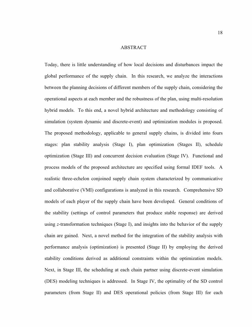
ABSTRACT

Today, there is little understanding of how local decisions and disturbances impact the

global performance of the supply chain. In this research, we analyze the interactions

between the planning decisions of different members of the supply chain, considering the

operational aspects at each member and the robustness of the plan, using multi-resolution

hybrid models. To this end, a novel hybrid architecture and methodology consisting of

simulation (system dynamic and discrete-event) and optimization modules is proposed.

The proposed methodology, applicable to general supply chains, is divided into fours

stages: plan stability analysis (Stage I), plan optimization (Stages II), schedule

optimization (Stage III) and concurrent decision evaluation (Stage IV). Functional and

process models of the proposed architecture are specified using formal IDEF tools. A

realistic three-echelon conjoined supply chain system characterized by communicative

and collaborative (VMI) configurations is analyzed in this research. Comprehensive SD

models of each player of the supply chain have been developed. General conditions of

the stability (settings of control parameters that produce stable response) are derived

using z-transformation techniques (Stage I), and insights into the behavior of the supply

chain are gained. Next, a novel method for the integration of the stability analysis with

performance analysis (optimization) is presented (Stage II) by employing the derived

stability conditions derived as additional constraints within the optimization models.

Next, in Stage III, the scheduling at each chain partner using discrete-event simulation

(DES) modeling techniques is addressed. In Stage IV, the optimality of the SD control

parameters (from Stage II) and DES operational policies (from Stage III) for each

19

member are concurrently evaluated by integrating the SD and DES models. Evaluation

in Stage IV is performed to better understand the global consequence of the locally

optimal decisions determined at each supply chain member. A generic infrastructure has

been developed using High Level Architecture (HLA) to integrate the distributed

decision and simulation models. Experiments are conducted to demonstrate the proposed

architecture for the analysis of distributed supply chains. The progressions of cost based

objective function from Stages I-III are compared with that from the concurrent

evaluation in Stage IV. Also the ability of the proposed methodology to capture the

effect of dynamic perturbations within the supply chain system is illustrated.

20

CHAPTER 1

INTRODUCTION

Successful supply chain management demands an effective cross-functional

coordination among the various business units of the supply chain. A supply chain can

be defined as a collection of business units or members that interact with one another to

transform raw materials to finished goods and distribute the finished goods to the

customers (Lee and Billington 1993, Swaminathan et al. 1995, Venkateswaran and Son

2004a). All the decisions in a supply chain involve interactions between multiple

departments across multiple business units. For example, the determination of the

optimal order quantity level by a manufacturer influences (and also depends on) the

suppliers’ production cycle time, choice of transportation, shipment sizes, capacity

requirements among others. Hence, it is observed that the supply chain members support,

interact or compete with each other to arrive at an overall optimum or equilibrium. Such

segregation and subsequent cooperation of decisions distributed over a range of business

units is commonly classified as distributed decision making.

In the context of a supply chain, two types of distributed decision making are

identified (Schneeweiss 2003) where, (1) the decision makers are spread across decision

levels (termed as vertical interactions), and (2) the decision makers are spread across

different members of the supply chain (termed as horizontal interactions). The former

refers to the influence of the strategic level decisions on the operational behavior and vise

21

versa of an organization. The latter refers to the influence and the possible need for

cooperation of decisions among the different members of the supply chain.

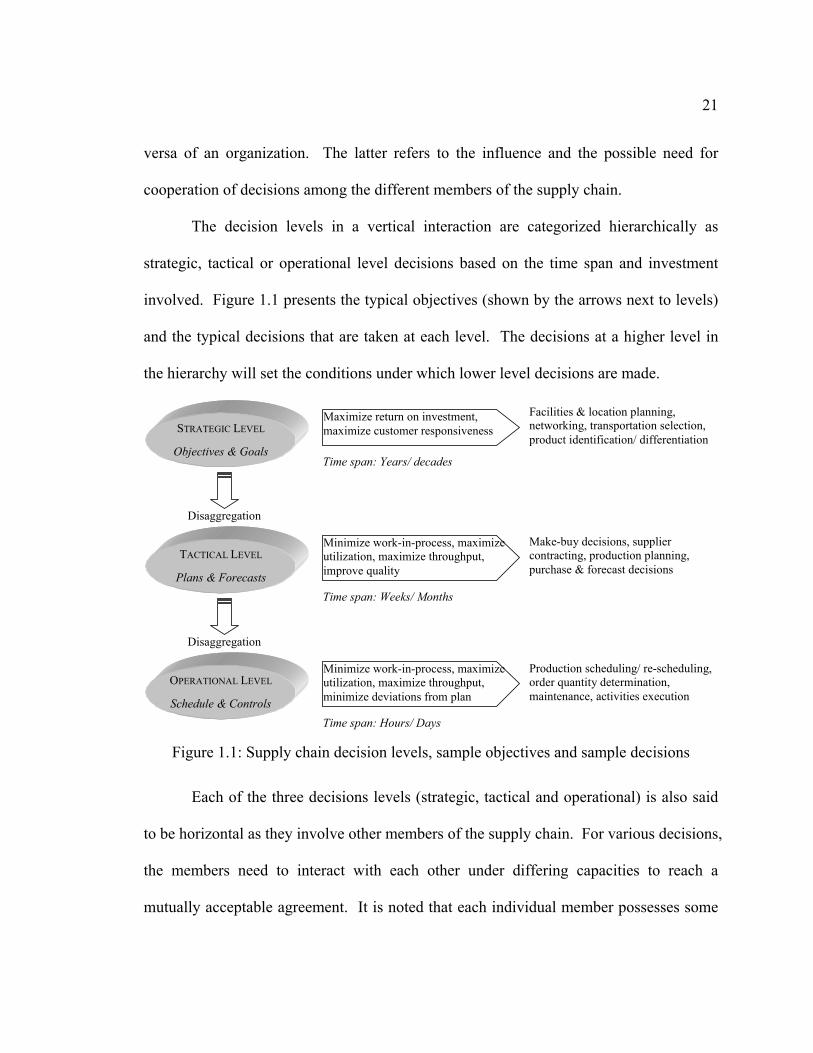
The decision levels in a vertical interaction are categorized hierarchically as

strategic, tactical or operational level decisions based on the time span and investment

involved. Figure 1.1 presents the typical objectives (shown by the arrows next to levels)

and the typical decisions that are taken at each level. The decisions at a higher level in

the hierarchy will set the conditions under which lower level decisions are made.

STRATEGIC LEVEL

Objectives & Goals

TACTICAL LEVEL

Plans & Forecasts

OPERATIONAL LEVEL

Schedule & Controls

Disaggregation

Disaggregation

Facilities & location planning, networking, transportation selection, product identification/ differentiation

Make-buy decisions, supplier contracting, production planning, purchase & forecast decisions

Production scheduling/ re-scheduling, order quantity determination, maintenance, activities execution

Time span: Years/ decades

Time span: Weeks/ Months

Time span: Hours/ Days

Maximize return on investment, maximize customer responsiveness

Minimize work-in-process, maximize utilization, maximize throughput, improve quality

Minimize work-in-process, maximize utilization, maximize throughput, minimize deviations from plan

Figure 1.1: Supply chain decision levels, sample objectives and sample decisions

Each of the three decisions levels (strategic, tactical and operational) is also said

to be horizontal as they involve other members of the supply chain. For various decisions,

the members need to interact with each other under differing capacities to reach a

mutually acceptable agreement. It is noted that each individual member possesses some

22

information which may be kept private and unshared with others or even falsely reported

to the other members. This further complicates the decision making process.

Both vertical and horizontal interactions occur simultaneously in a supply chain.

For instance, consider that the strategic decision of the marketing department of the

manufacturer is to sell high-end customer oriented products. This influences the

selection of the suppliers (based on quality of products, or on-time delivery rate),

planning and location of warehouse and distribution centers, choice of transportation

(road/ sea/ air, depending on how efficiently the finished product is delivered to the

customer), among others. This illustrates the horizontal nature of strategic decisions

which involve multiple players of the supply chain. The above mentioned strategic

decision of the manufacturer also influences the tactical decisions such as production

planning (make-to-order will be preferred over made-to-stock) and make-or-buy

decisions, which further influences the operational decisions such as setting quality

control limits on the various components. Thus, decisions at the strategic level have an

effect on the decisions at the tactical and operational levels. The tactical and operational

decisions are also horizontal as they spread across multiple supply chain players, as

mentioned earlier.

In this research, the interaction between the planning and operational decisions

that are spread across multiple decisions levels and multiple members of the supply chain

are analyzed. Hierarchical Production Planning (HPP) decisions that are spread across

multiple decision levels are employed. The interactions between the multiple members

of the supply chain are based on the configuration of the supply chain. Two supply chain

23

configurations are together considered: (1) communicative configuration, in which the

members interact in a traditional manner and exchange only the order data, and (2)

collaborative configuration, in which the members work together on a particular business

function. The collaborative configuration considered in this research is Vendor Managed

Inventory.

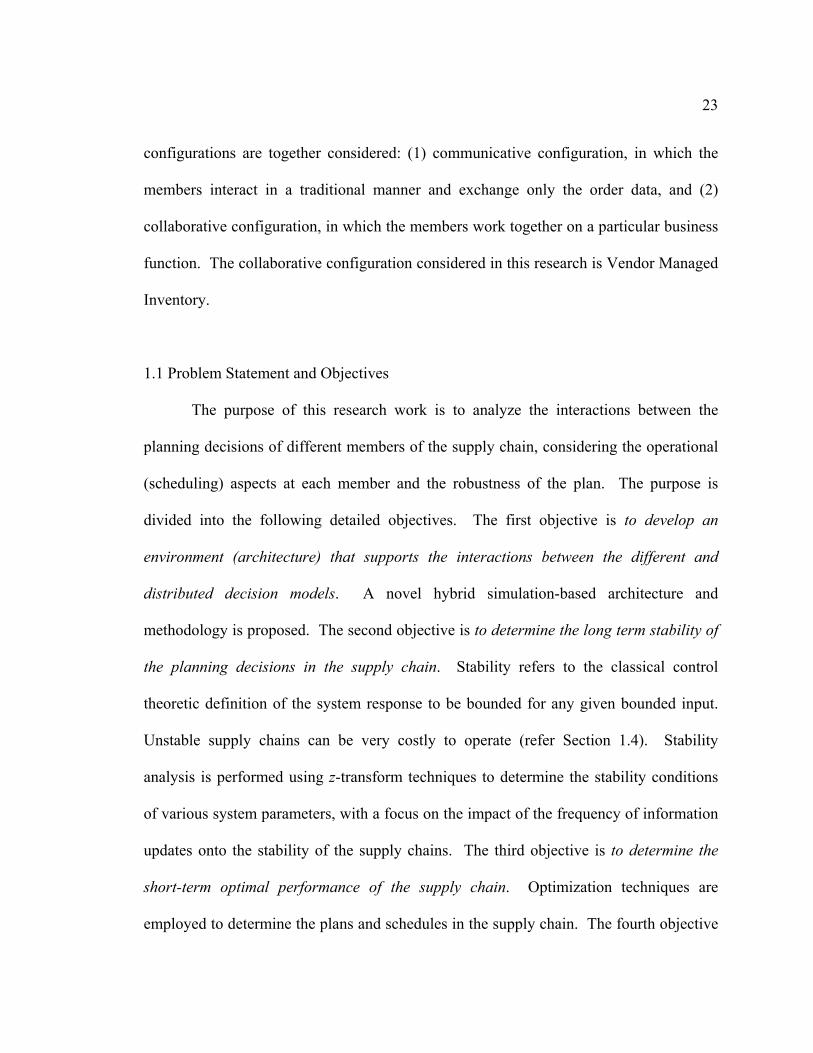
1.1 Problem Statement and Objectives

The purpose of this research work is to analyze the interactions between the

planning decisions of different members of the supply chain, considering the operational

(scheduling) aspects at each member and the robustness of the plan. The purpose is

divided into the following detailed objectives. The first objective is to develop an

environment (architecture) that supports the interactions between the different and

distributed decision models. A novel hybrid simulation-based architecture and

methodology is proposed. The second objective is to determine the long term stability of

the planning decisions in the supply chain. Stability refers to the classical control

theoretic definition of the system response to be bounded for any given bounded input.

Unstable supply chains can be very costly to operate (refer Section 1.4). Stability

analysis is performed using z-transform techniques to determine the stability conditions

of various system parameters, with a focus on the impact of the frequency of information

updates onto the stability of the supply chains. The third objective is to determine the

short-term optimal performance of the supply chain. Optimization techniques are

employed to determine the plans and schedules in the supply chain. The fourth objective

24

is to evaluate the effect of interactions between the decision models in different levels and

across different members. This is performed to better understand the global consequences

of the locally optimal decisions determined at each decision model. The fifth objective is

to develop the infrastructure to enable distributed analysis of system of systems. The

decisions models at different supply chain members are themselves complex systems, and

this research work is concerned with the functioning of the system of systems. Generic

infrastructure is developed using High Level Architecture (HLA). An additional final

objective is identified to demonstrate the functioning of the proposed architecture for

different supply chain configurations.

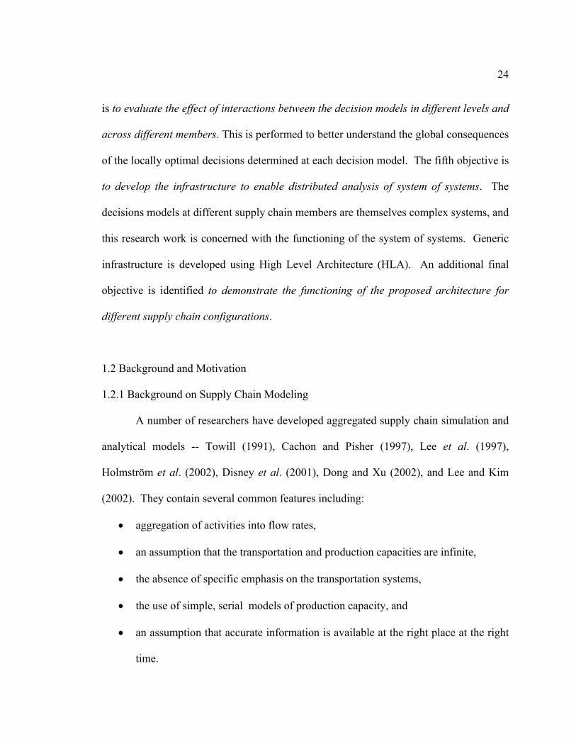
1.2 Background and Motivation

1.2.1 Background on Supply Chain Modeling

A number of researchers have developed aggregated supply chain simulation and

analytical models -- Towill (1991), Cachon and Pisher (1997), Lee et al. (1997),

Holmström et al. (2002), Disney et al. (2001), Dong and Xu (2002), and Lee and Kim

(2002). They contain several common features including:

• aggregation of activities into flow rates,

• an assumption that the transportation and production capacities are infinite,

• the absence of specific emphasis on the transportation systems,

• the use of simple, serial models of production capacity, and

• an assumption that accurate information is available at the right place at the right

time.

25

These assumptions and approximations, in our opinion, limit the predictive capability of

these models. For example, Venkateswaran and Son (2004a) found that supply-chain

performance predictions were more sensitive to approximations in delays and capacities

in the models than forecasts of end customer demand. Furthermore, the effect of the

global supply chain decisions on the individual member performance of individual chain

members has not been analyzed.

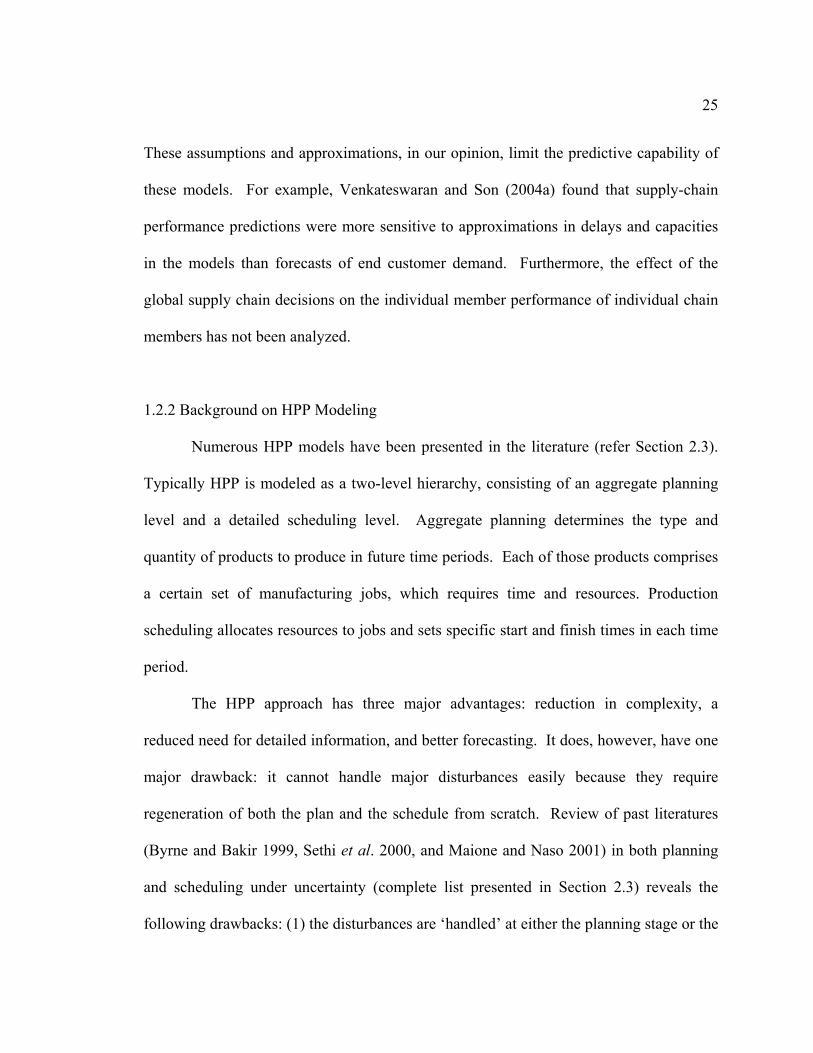
1.2.2 Background on HPP Modeling

Numerous HPP models have been presented in the literature (refer Section 2.3).

Typically HPP is modeled as a two-level hierarchy, consisting of an aggregate planning

level and a detailed scheduling level. Aggregate planning determines the type and

quantity of products to produce in future time periods. Each of those products comprises

a certain set of manufacturing jobs, which requires time and resources. Production

scheduling allocates resources to jobs and sets specific start and finish times in each time

period.

The HPP approach has three major advantages: reduction in complexity, a

reduced need for detailed information, and better forecasting. It does, however, have one

major drawback: it cannot handle major disturbances easily because they require

regeneration of both the plan and the schedule from scratch. Review of past literatures

(Byrne and Bakir 1999, Sethi et al. 2000, and Maione and Naso 2001) in both planning

and scheduling under uncertainty (complete list presented in Section 2.3) reveals the

following drawbacks: (1) the disturbances are ‘handled’ at either the planning stage or the

26

scheduling stage, with little or no interaction between the stages, and (2) Similar sources

of disturbances are handled separately by the planning and scheduling modules. The

impact of local planning and scheduling decisions on the global performance has not

been analyzed.

1.2.3 Motivation

In the case of supply chains, the effect of the global behavior of the supply chain

on the individual member performance has not been analyzed. In the case of HPP, the

impact of planning and scheduling decisions of a member on the global performance has

not been analyzed. The need for the study of such interactions between the internal

workings of a member along with the global performance of the supply chain motivated

this research work.

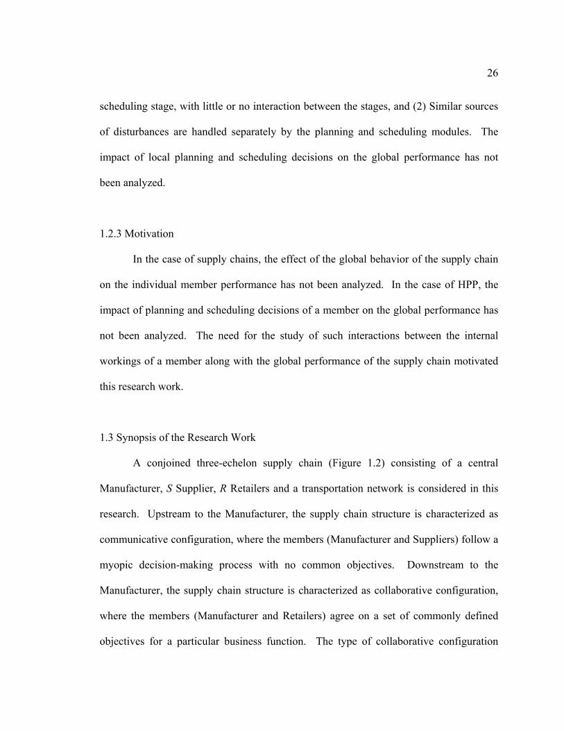
1.3 Synopsis of the Research Work

A conjoined three-echelon supply chain (Figure 1.2) consisting of a central

Manufacturer, S Supplier, R Retailers and a transportation network is considered in this

research. Upstream to the Manufacturer, the supply chain structure is characterized as

communicative configuration, where the members (Manufacturer and Suppliers) follow a

myopic decision-making process with no common objectives. Downstream to the

Manufacturer, the supply chain structure is characterized as collaborative configuration,

where the members (Manufacturer and Retailers) agree on a set of commonly defined

objectives for a particular business function. The type of collaborative configuration

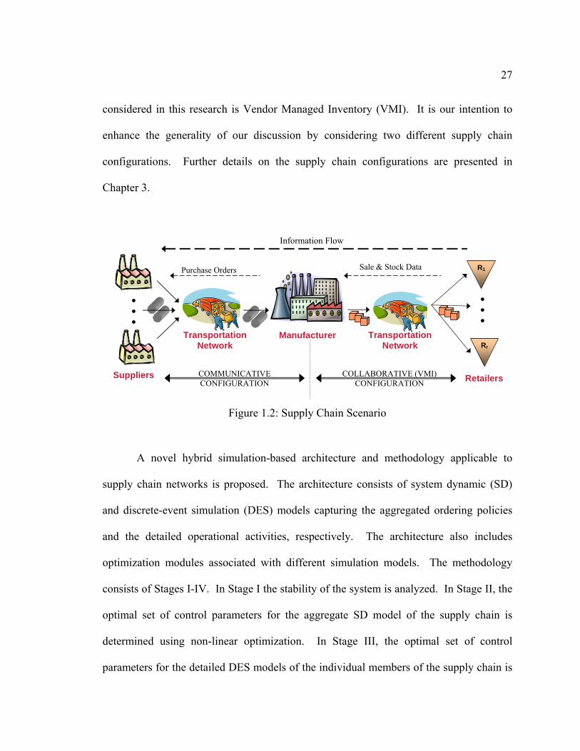
27

considered in this research is Vendor Managed Inventory (VMI). It is our intention to

enhance the generality of our discussion by considering two different supply chain

configurations. Further details on the supply chain configurations are presented in

Chapter 3.

Suppliers

Manufacturer

Retailers

R1

Rr

TransportationNetwork

Information Flow

COMMUNICATIVE CONFIGURATION

Purchase Orders Sale & Stock Data

COLLABORATIVE (VMI) CONFIGURATION

Transportation Network

Figure 1.2: Supply Chain Scenario

A novel hybrid simulation-based architecture and methodology applicable to

supply chain networks is proposed. The architecture consists of system dynamic (SD)

and discrete-event simulation (DES) models capturing the aggregated ordering policies

and the detailed operational activities, respectively. The architecture also includes

optimization modules associated with different simulation models. The methodology

consists of Stages I-IV. In Stage I the stability of the system is analyzed. In Stage II, the

optimal set of control parameters for the aggregate SD model of the supply chain is

determined using non-linear optimization. In Stage III, the optimal set of control

parameters for the detailed DES models of the individual members of the supply chain is

28

determined. In Stage IV, the optimality of the SD control parameters (from Stage II) and

DES operational policies (from Stage III) for each member are concurrently evaluated by

integrating the SD and DES models. Evaluation in Stage IV is performed to better

understand the global consequence of the locally optimal decisions determined at each

supply chain member. It is noted that the hybrid integrated models cannot be directly

used in stability analysis or optimization due to (1) the varied and often conflicting

objectives for the different members and the different levels (planning and scheduling),

(2) the complexity in building the models, especially the DES models that contain the

detailed operational activities of the members, and (3) time involved in executing the

entire distributed structure. The applicability of the architecture for the supply chain

scenario considered is presented in Chapter 3. Also, formal models are developed using

Integrated DEFinition (IDEF) tools to unambiguously describe the proposed architecture

and methodology (refer Chapter 3).

The models developed (specific contributions of this research) capture (1) the

mixing and variability in the production process and the production lead time, (2)

capacitated resource allocation, (3) order backlog, (4) frequency of information update,

(5) raw material component inventory, (6) transportation network, and (5) provides for

spatial and lateral dimension of the supply chain. The models of individual members of

the supply chain are defined conceptually using modified causal loop diagrams (CLD),

and differential equation models (and later into difference equation models) which can be

readily simulated. The details of the models can be found in Chapter 4. It is noted that

differential equation models provide more accuracy as they represent time as unfolding

29

continuously (Sterman 2000). That is, time progresses smoothly and continuously, and

event can happen at any time. Now, further analysis (stability and optimization) and even

data collection for a supply chain system requires time to be quantized into intervals.

Hence, the differential equations are translated into difference equation models. In this

research, the models are initially defined using differential equations (Chapter 4), and

then converted into difference equations for use in the rest of the dissertation (Chapters 5-

9).

Dynamic behavior and the conditions for stability for the supply chain system is

analyzed, as part of Stage I activities (Chapter 5). The general conditions for stability of

the supply chain are derived and the effects of intra-player sampling interval and inter-

player sampling intervals have been analyzed using z-transform techniques. Guidance for

the selection of appropriate parameters (especially, the frequency of information update)

depending on the supply chain characteristics (communicative vs. collaborative) to

guarantee stability is presented. The reasons for including stability analysis are discussed

in Section 1.4.

In Stage II, the aggregate level SD models are optimized using non-linear

optimization techniques. A novel method for the integration of the stability analysis with

performance analysis (optimization) is presented by employing the stability conditions

derived in Stage I as additional constraints within the optimization models. The need for

such integration is highlighted through preliminary experiments, the details of which can

be found in Chapter 6. The reasons for combining stability and performance analysis are

presented in Section 1.4.

30

Descriptions are presented for the modeling of the detailed models using Discrete

Event Simulation (DES). The schedule optimization (Stage III) is described by

presenting the decision variables, objective functions and the optimization methodology.

The specifications for interactions of the SD and DES models, for use in Stage IV of the

proposed architecture are detailed. Unlike the typical interaction between aggregate and

detailed models (in which each model is run sequentially for the full time horizon), in this

research the models interact every time periods (run concurrently), allowing for the

supply chain system to evolve concurrently. Details on the inclusion of the detailed

models in supply chain analysis are presented in Chapter 7.

Implementation wise, the non-linear optimization problems are solved using

AMPL® and solver MINOS® 5.5. The SD models are implemented using Powersim®

2.51. The DES models are built using Arena® 8.0. A generic infrastructure has been

developed using High Level Architecture (HLA) to integrate and together simulate the

distributed simulation models. The details of implementation can be found in Chapter 8.

Experiments are conducted to demonstrate the proposed hybrid simulation-based

architecture for the analysis of supply chains. Separate results for communicative

configuration supply chain and collaborative (VMI) configuration supply chain are

presented. Also the ability of the proposed methodology to capture the effect of dynamic

perturbations within the supply chain system is illustrated. Complete report on the

experiments is presented in Chapter 9.

31

1.4 Justification of Selected Methods and Techniques

• Why have you proposed a new architecture and methodology?

Given the scope of this research, the effects of detail-level operational policies on

the aggregate-level planning policies are to be analyzed. Also, effects of decisions

within the individual members of the supply chain on other members; and the

resulting global performance of the supply chain are to be studied. The models

employed involve varying levels of detail, with the ability to capture the dynamic

behavior of the supply chain. From the perspective of techniques employed,

performance analysis (optimization) is integrated with stability analysis. The non-

availability of an architecture and methodology enabling the required analysis forced

the development of a new architecture / methodology.

• Why have you used system dynamics models? Can’t I just use discrete-event models

to capture the SD model?

SD models represent the aggregate level planning decisions and the DES models

represent the detailed operational activities at each member of the supply chain. At

the aggregate level, the decisions made (such as determination of production release

rates) require the use of various system parameters (such as inventory, and demand).

Hence the relationships between the different system parameters need to be explicitly

modeled. Also, since the production systems within the supply chain are dynamic

evolutionary systems, a time-based dynamic model is required. Due to the

evolutionary nature, a decision taken at one point in time influences the decisions at

32

later points in time. This results in feedback structured model of the supply chain

system. System dynamic provides the required framework to capture the aggregate-

level model adequately and hence used in this research. The properties or core

factors of SD modeling includes (Reid and Koljonen 1999): (1) the structure of the

system can be expressed in the form of feedback-based causal loop diagrams, (2) the

frequency and duration of time delays in the feedback loops, and (3) the amplification

of the information flows through the feedback structure can be captured. Also, SD

model explicitly support the analysis of system stability. It is noted that DES

environment can be used to represent a dynamic model of the system. This would

require a significant amount of customization of the DES environment and yet the

models developed will still be classified as system dynamic models since the concepts

of interrelating the variables is based on system dynamics.

• Why do you combine stability analysis and performance analysis (optimization)?

The supply chain is a closed loop system with the typical flow of materials

downstream and the typical flow of information upstream. The responses of such a

closed loop system on the long term could result in unstable behavior of the supply

chain over time. Unstable supply chains will experience large swings in demand,

periods of shortage in materials and products, periods of excess stock of materials,

unpredictable lead times, all of which affects the long term profits and success of the

supply chain. Hence, a desired feature of the supply chain decision policies is their

ability to stabilize the system response. Now, it is also desired to find out which is

33

the most cost effective decisions for the supply chain in the near term, which lead to

the use of optimization techniques. Hence, in this research, performance and stability

analysis are combined, by employing the long-term stability conditions within the

short-term optimization. The validity of the approach is discussed in Chapter 6.

• Why should the models be distributed?

Various legacy models representing the different activities at the different

decisions levels are available with the supply chain members. It is desirable to take

advantage of such existing system models. Hence, it is the presence of the various

distributed models, and the very distributed nature of the supply chains that lead to

development of the architecture that supports distributed modeling and analysis (and

not the other way around). Also, the use of distributed models allows each supply

chain member to hide any proprietary information in implementation of the individual

models, but still provide enough information to evaluate the supply chain as a whole.

Thus, the proposed architecture and methodology enable the development and

analysis of systems of systems.

1.5 Organization of the Remainder of the Thesis

The remainder of the thesis is organized as follows. Chapter 2 provides an

introduction to supply chains and summarizes the literature survey of the previous works

in stability analysis of supply chains, hierarchical production planning and hybrid

simulation systems. Chapter 3 presents the detailed description of the supply chain

34

scenario along with the proposed architecture and methodology to analyze the supply

chain. In Chapter 4, the aggregate-level SD models used in the planning stage of the

different members of the supply chain are described. In Chapter 5 (Stage I), the general

conditions for stability of the supply chain are derived and the effects of intra-player

sampling interval and inter-player sampling intervals are analyzed. The integrated

performance and stability analysis (Stage II) of the aggregate SD models and the

validation of the same are presented in Chapter 6. In Chapter 7, the need for the

inclusion of detailed models in the supply chain analysis is discussed. The DES model

descriptions and the schedule optimization (Stage III) are described. Also, the

specifications for interactions of the SD and DES models, for use in Stage IV of the

proposed architecture are detailed. In Chapter 8, the generic infrastructure developed to

integrate and together simulate the distributed models is described. Experiments to

demonstrate the proposed hybrid simulation-based architecture for the analysis of supply

chains is presented in Chapter 9. Chapter 10 includes a summary of the findings and the

conclusions drawn for this research. The directions of future research are also indicated.

35

CHAPTER 2

LITERATURE REVIEW

In this chapter, the extensive literature review conducted is summarized. First, a

brief background on supply chain, their structure and decisions is presented. Next,

background on the stability analysis in supply chains and production-inventory systems is

presented. Past research works in the area of HPP, especially in the stochastic

manufacturing environment, are then summarized.

2.1 Background on Supply Chain

2.1.1 Definitions

A supply chain is a collection of business units that interact with one another to

transform raw materials into finished goods and distribute the finished goods to the

customers (Lee and Billington 1993, Ganeshan and Harrison 1995, Swaminathan et al.

1995, Mabert and Venkataramanan 1998, Bhaskaran 1998). The typical business units of

a supply chain can be grouped into suppliers/vendors, distribution centers, manufacturing

plants, transportation network, warehouses, and retailers/customers. Traditionally, the

various business units along the supply chain operate independently. These units have

their own, often conflicting, objectives (Ganeshan and Harrison 1995). This calls for a

plan to coordinate the different business units within the supply chain for effective

management. Such an integration strategy is called supply chain management. A fine

demarcation can be drawn between supply chain and supply chain management. The

36

former is a collection of business units, while the latter takes over the management efforts

of the business units within the supply chain (Mentzer 2000). The common thread in any

definition of supply chain management is that it seeks to integrate performance measures

over multiple firms or processes, rather than taking the perspective of a single firm or

process (Houlihan 1985, Cooper et al. 1997, Lambert et al. 1998).

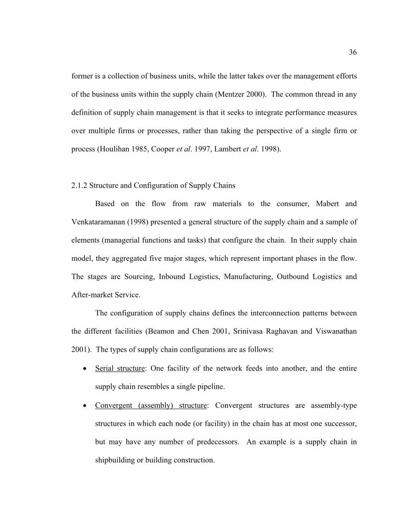
2.1.2 Structure and Configuration of Supply Chains

Based on the flow from raw materials to the consumer, Mabert and

Venkataramanan (1998) presented a general structure of the supply chain and a sample of

elements (managerial functions and tasks) that configure the chain. In their supply chain

model, they aggregated five major stages, which represent important phases in the flow.

The stages are Sourcing, Inbound Logistics, Manufacturing, Outbound Logistics and

After-market Service.

The configuration of supply chains defines the interconnection patterns between

the different facilities (Beamon and Chen 2001, Srinivasa Raghavan and Viswanathan

2001). The types of supply chain configurations are as follows:

• Serial structure: One facility of the network feeds into another, and the entire

supply chain resembles a single pipeline.

• Convergent (assembly) structure: Convergent structures are assembly-type

structures in which each node (or facility) in the chain has at most one successor,

but may have any number of predecessors. An example is a supply chain in

shipbuilding or building construction.

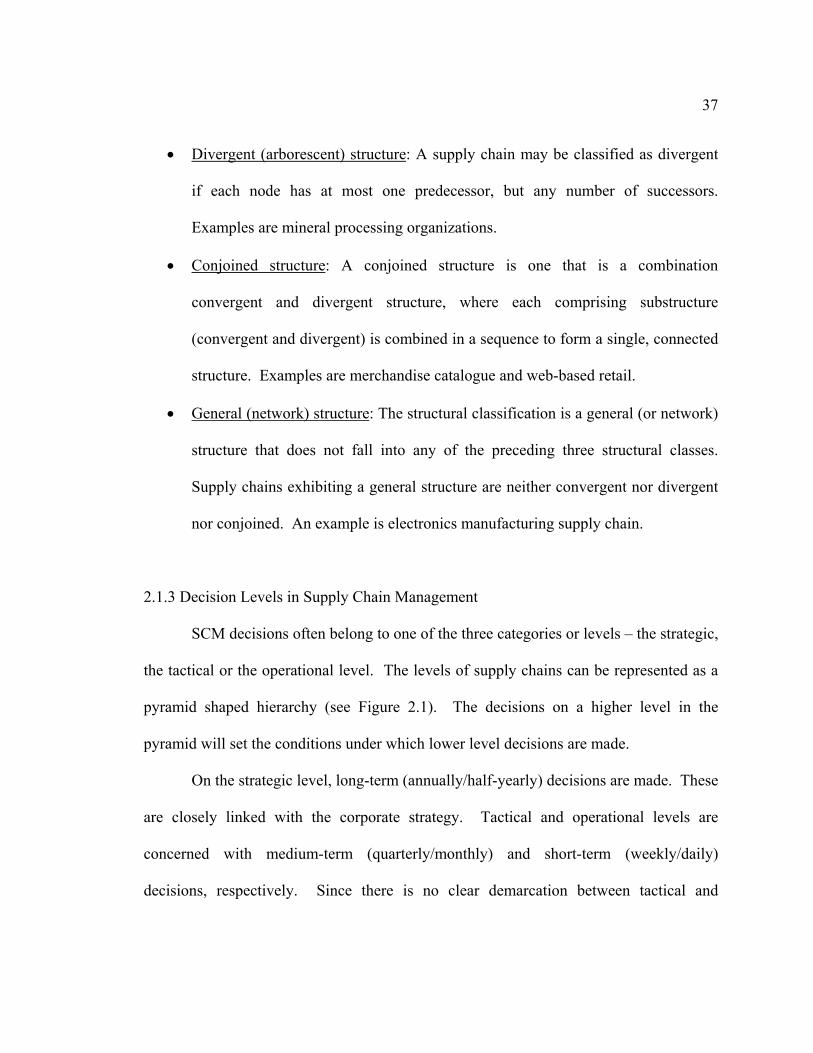
37

• Divergent (arborescent) structure: A supply chain may be classified as divergent

if each node has at most one predecessor, but any number of successors.

Examples are mineral processing organizations.

• Conjoined structure: A conjoined structure is one that is a combination

convergent and divergent structure, where each comprising substructure

(convergent and divergent) is combined in a sequence to form a single, connected

structure. Examples are merchandise catalogue and web-based retail.

• General (network) structure: The structural classification is a general (or network)

structure that does not fall into any of the preceding three structural classes.

Supply chains exhibiting a general structure are neither convergent nor divergent

nor conjoined. An example is electronics manufacturing supply chain.

2.1.3 Decision Levels in Supply Chain Management

SCM decisions often belong to one of the three categories or levels – the strategic,

the tactical or the operational level. The levels of supply chains can be represented as a

pyramid shaped hierarchy (see Figure 2.1). The decisions on a higher level in the

pyramid will set the conditions under which lower level decisions are made.

On the strategic level, long-term (annually/half-yearly) decisions are made. These

are closely linked with the corporate strategy. Tactical and operational levels are

concerned with medium-term (quarterly/monthly) and short-term (weekly/daily)

decisions, respectively. Since there is no clear demarcation between tactical and

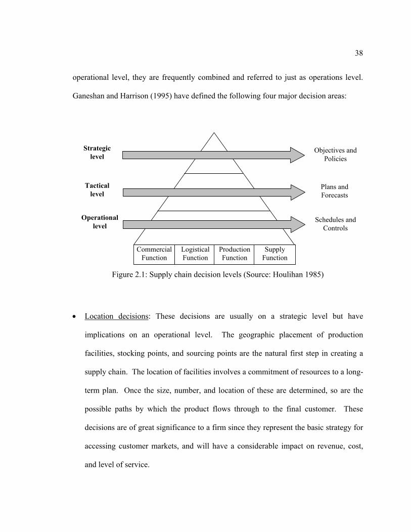
38

operational level, they are frequently combined and referred to just as operations level.

Ganeshan and Harrison (1995) have defined the following four major decision areas:

Strategic level

Tactical level

Operational level

Objectives and Policies

Plans and Forecasts

Schedules and Controls

Commercial Function

Logistical Function

Production Function

Supply Function

Figure 2.1: Supply chain decision levels (Source: Houlihan 1985)

• Location decisions: These decisions are usually on a strategic level but have

implications on an operational level. The geographic placement of production

facilities, stocking points, and sourcing points are the natural first step in creating a

supply chain. The location of facilities involves a commitment of resources to a long-

term plan. Once the size, number, and location of these are determined, so are the

possible paths by which the product flows through to the final customer. These

decisions are of great significance to a firm since they represent the basic strategy for

accessing customer markets, and will have a considerable impact on revenue, cost,

and level of service.

39

• Production decisions: These decisions are on a strategic, tactical as well as

operational level. The strategic decisions include what products to produce, and

which plants to produce them in, allocation of suppliers to plants, plants to

distribution centers, and distribution center’s to customer markets. These decisions

have a big impact on the revenues, costs and customer service levels of the firm.

These decisions assume the existence of the facilities, but determine the exact path(s)

through which a product flows to and from these facilities. Another critical issue is

the capacity of the manufacturing facilities, and this largely depends on the degree of

vertical integration within the firm. Operational decisions focus on detailed

production scheduling. These decisions include the construction of the master

production schedules, scheduling production on machines, and equipment

maintenance. Other considerations include workload balancing, and quality control

measures at a production facility.

• Inventory decisions: These refer to the means by which inventories are managed.

Inventories exist at every stage of the supply chain as either raw material, semi-

finished or finished goods. They can also be in process between locations. Their

primary purpose is to buffer against any uncertainty that might exist in the supply

chain. Their efficient management is critical in supply chain operations. Inventory

decisions are strategic in the sense that the top management sets goals. However,

most researchers have approached the management of inventory from an operational

perspective. These include deployment strategies (push versus pull), control policies

40

- the determination of the optimal levels of order quantities and reorder points, and

setting safety stock levels, at each stocking location.

• Transport decisions: The mode choice aspects of these decisions are the more

strategic ones. These are closely linked to the inventory decisions, since the best

choice of mode is often found by trading-off the cost of using the particular mode of

transport with the indirect cost of inventory associated with that mode. While air

shipments may be fast, reliable, and warrant lesser safety stocks, they are expensive.

Meanwhile shipping by sea or rail may be much cheaper, but they necessitate holding

relatively large amounts of inventory to buffer against the inherent uncertainty

associated with them. Therefore, customer service levels and geographic location

play vital roles in such decisions. Since transportation is more than 30 percent of the

logistics costs, operating it efficiently makes good economic sense. Shipment sizes

(consolidated bulk shipments versus Lot-for-Lot), routing and scheduling of pieces of

equipment are the key in effective management of the firm's transport strategy.

In this dissertation, a three echelon conjoined supply chain is analyzed. Also, the

decisions of interest includes the production and inventory decisions at the tactical and

operational levels

2.2 Stability Analysis in Supply Chains

This dissertation analyzes the stability of supply chain systems. A comprehensive

literature review on the use of control theoretic concepts for the dynamic analysis of

41

production – inventory systems can be found in Ortega and Lin (2004) and in Disney and

Towill (2002). John et al. (1994) demonstrated the stabilizing effect of including a

supply line (WIP) component into an inventory and order based production control

system (Towill 1982), using block diagrams and Laplace transform. Towill et al. (1997)

examined the critical design parameters within an adaptive model consisting of three

feedback loops – inventory error loop, desired order in pipeline loop and the lead time

loop, and highlighted how the total orders in the pipeline can be used for assessing the

load of the internal manufacturing pipeline. Grubbström (1998) used Laplace transform,

z-transform and Net Present Value on MRP systems and showed a three-fold use of

transfer functions: (1) describes production, demand and inventory dynamics in a

compact way, (2) captures stochastic properties by serving as moment generating

functions, and (3) assesses the cash flows up capturing the net present value in the

transfer functions. White (1999) has showed that simple inventory management systems

are analogous to the proportional control in conventional control theory, and has

demonstrated the use proportional, integrative and derivative (PID) control algorithms

can result in saving of up to 80%.

Optimal control parameters for use in general production and inventory control

systems have been found by Disney et al. (2000) using genetic algorithm. The

performance measures characteristics considered by them include (1) inventory recovery

to "shock" demands, (2) in-built filtering capability, (3) robustness to the production lead-

time variations, (4) robustness to pipeline level information fidelity, and (5) systems

selectivity. Dejonckheere et al. (2003) have employed filter theory to relate the dynamics

42

of order replenishment to the production planning strategies ranging from lean systems to

agile systems, highlighting the flexibility of their order replenishment policy. Disney et

al. (2004) have studied a general production-inventory control system which is

guaranteed to be stable through the use of Deziel-Eilon arbitrary setting (Deziel and Eilon

1967). They have derived analytical expressions for the bullwhip and inventory variance

produced by the control system, and highlighted the bullwhip boundary as a function of

the inventory feedback gain. Using linear z-transform analysis, Disney and Towill (2005)

have identified and proposed a method to eliminate the possibility of an inventory drift

and instability due to uncertain pipeline lead times.

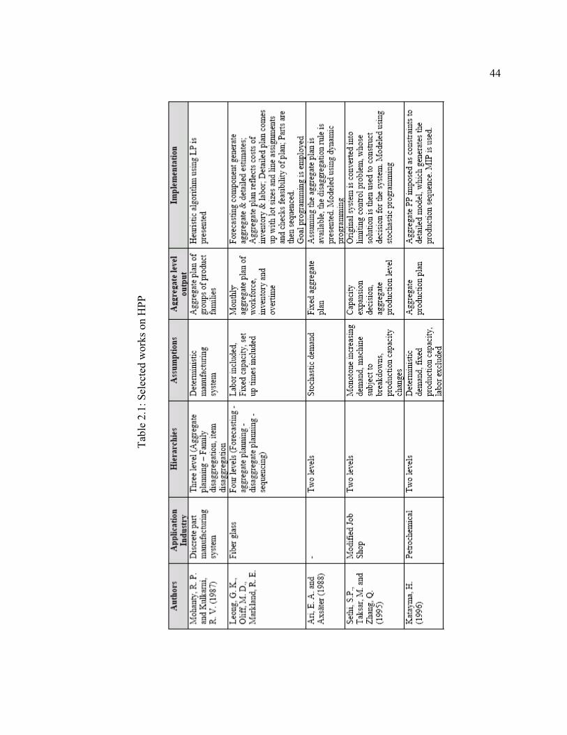
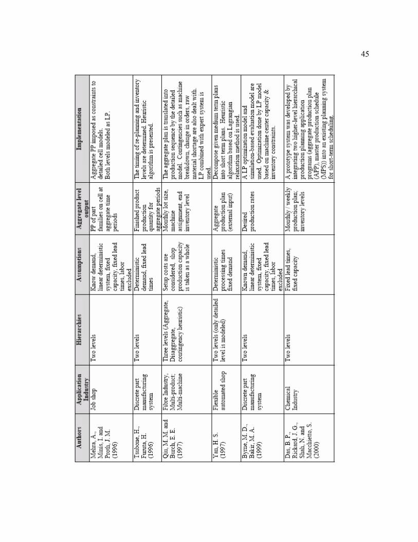
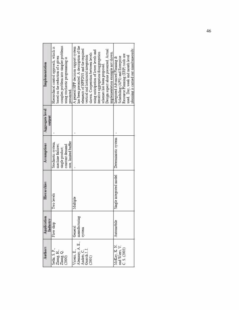
2.3 Hierarchical Production Planning

This dissertation includes concepts of hierarchical production planning (HPP)

system. Past research works in the area of HPP, especially in the stochastic

manufacturing environment, are summarized in Table 2.1 using five attributes of

classification that we have identified. First, the application industry attribute identifies

the type of manufacturing system for which the HPP is developed. Second, the number

of hierarchies identified and modeled is shown. Typically, it is found that the HPP is

restricted to two levels of planning and scheduling. Third, the specific assumptions with

regards to the demand, manufacturing capacity and disturbances considered are presented.

Fourth, the output of the higher aggregate planning level is shown. The output is

predominantly the aggregate production plan where the products are grouped into product

families and time is aggregated into weeks or months. The final attribute highlights the

43

method employed in implementing the HPP. Works have been presented such that the

methodology varies from linear programming to stochastic models to heuristics and

simulation based approaches.

44

Tabl

e 2.

1: S

elec

ted

wor

ks o

n H

PP

47

Vicens et al. (2001) highlights several drawbacks of such methods.

• The use of deterministic data at the aggregate level does not account for the stochastic

evolution of the actual system. Usually worst-case performance data are used at the

aggregate level, leading to feasible but not optimal solutions. In addition, the

dynamics of the underlying system are absent.

• Models assume infinite capacity and hence performance is assumed to remain

constant irrespective of workload. This implies that, Little’s Law (which states that

Work-in-Progress = Throughput * Cycle time) may be violated.

• Major drawback of the techniques is that they require reruns in the case of unexpected

external or internal events (Vicens et al. 2001). Any exception (such as machine

failures, new order arrivals) that endangers the validity of the current production plan

leads to the regeneration of the entire plan.

• The solutions of the models are optimal and valid only when the assumptions are true.

Since the dynamics of the actual system is not accounted for, optimality is certainly

questionable.

• The models are suitable only for simple planning scenarios. For more realistic

scenarios, the sequential solution approach may lead to sub-optimality, inconsistency,

or infeasibility (Vicens et al. 2001).

The above drawbacks of existing methods also motivated this research in which, dynamic

models are used to represent the planning and scheduling decisions.

48

2.4 Hybrid Simulation Systems

In this dissertation, hybrid system dynamic – discrete event simulation has been

employed for analysis of the supply chain. Past work in the areas of hybrid and

distributed simulation are presented in this section. Hybrid simulation refers to the work

carried out in using together discrete and continuous aspects for analyzing a system.

Distributed simulation concerns itself with the work done in the integration of multiple

simulation models.

Architecture for hybrid simulation using Simple++ and SAM simulator, to model

the discrete and continuous aspects of a FMS respectively, has been presented by

Petropoulakis and Giacomini (1998). Another framework of discrete-continuous

combined modeling for a supply chain system is proposed by Lee et al. (2002). They

represented the continuous aspects of the supply chain (such as ordering rate, shipping

rate and inventory) using mathematical equations, which is then integrated with the

discrete aspects of the supply chain such as transportation activity. The results of this

combined approach were appraised to that of a discrete-event simulation model. Rabelo

et al. (2003) presented the potential merit of integrating SD and DES models to evaluate

the impact of local production decision on the global enterprise. However, integration of

the simulations in terms of time and information coordination was not addressed.

Venkateswaran and Son (2004c) have highlighted a need for an integrated hybrid SD-

DES simulation environment. An initial feasibility analysis has been carried out in which

the inventory management aspects of a facility are modeled using SD and the shop floor

operations are modeled using DES. Later, Venkateswaran et al. (2004) described a two

49

level HPP architecture consisting of SD components at the higher decision level and DES

components at the lower decision level. Venkateswaran and Son (2004d) showed the

applicability of their approach to a multi-product discrete part manufacturing enterprise

and provided formal descriptions of their architecture for HPP analysis within a single

enterprise in IDEF∅. The authors (1) described the functions of the different modules in

the architecture along with the integration strategies, and (2) demonstrated the validity of

the approach with experimental results.

The use of multiple simulation models in analyzing complex systems requires an

effective interfacing of multiple simulations. Several works has been presented in

describing framework architecture, communication requirements, protocols and

algorithms for coordinating and interfacing the multiple simulations (Kaacutedaacuter et

al. 1998, Fujimoto 2000, Zeigler and Sarjoughian 2000, Taylor et al. 2002). The High

Level Architecture (HLA) has become the de-facto standard in distributed simulation

(Kuhl et al. 1999, McLean and Riddick 2000). Venkateswaran and Son (2004b) have

addressed the application of distributed simulation technology to evaluate potential

supply chains. They presented information models for enabling distributed simulation of

multiple discrete event simulation models, each representing a member of the supply

chain. The HLA Run Time Infrastructure (RTI) had been used to provide an interface to

create the distributed simulation system.

50

CHAPTER 3

SUPPLY CHAIN SCENARIO, PROPOSED ARCHITECTURE AND

METHODOLOGY

In this chapter, the supply chain scenario along with the proposed architecture and

methodology to analyze the supply chain are presented. First, an overview of the supply

chain scenario is presented, followed by the general description of the proposed

architecture and methodology. Next, the applicability of the proposed architecture to the

supply chain scenario under scrutiny is explored. Formal techniques (IDEFØ and

IDEF3) are employed to unambiguously describe the functional components and process

models of the proposed architecture. The detailed descriptions of the supply chain and

the shop floor layouts of the Suppliers and Manufacturer are also presented.

3.1 Overview of Supply Chain Scenario

The supply chain system considered in this research consists of a central

Manufacturer, S Suppliers, R Retailers and a Transportation network (see Figure 3.1). N

products are handled by the supply chain, the demands for which exist at all the Retailers.

The end customer places orders to and receives the products from the Retailers. The

Manufacturer produces the N products and supplies them to the Retailers. The bill-of-

materials of the products is composed of M components that are obtained from the

Suppliers which manufacture the components. Infinite supply of raw materials for

component production is assumed to be available with the Suppliers. The Transportation

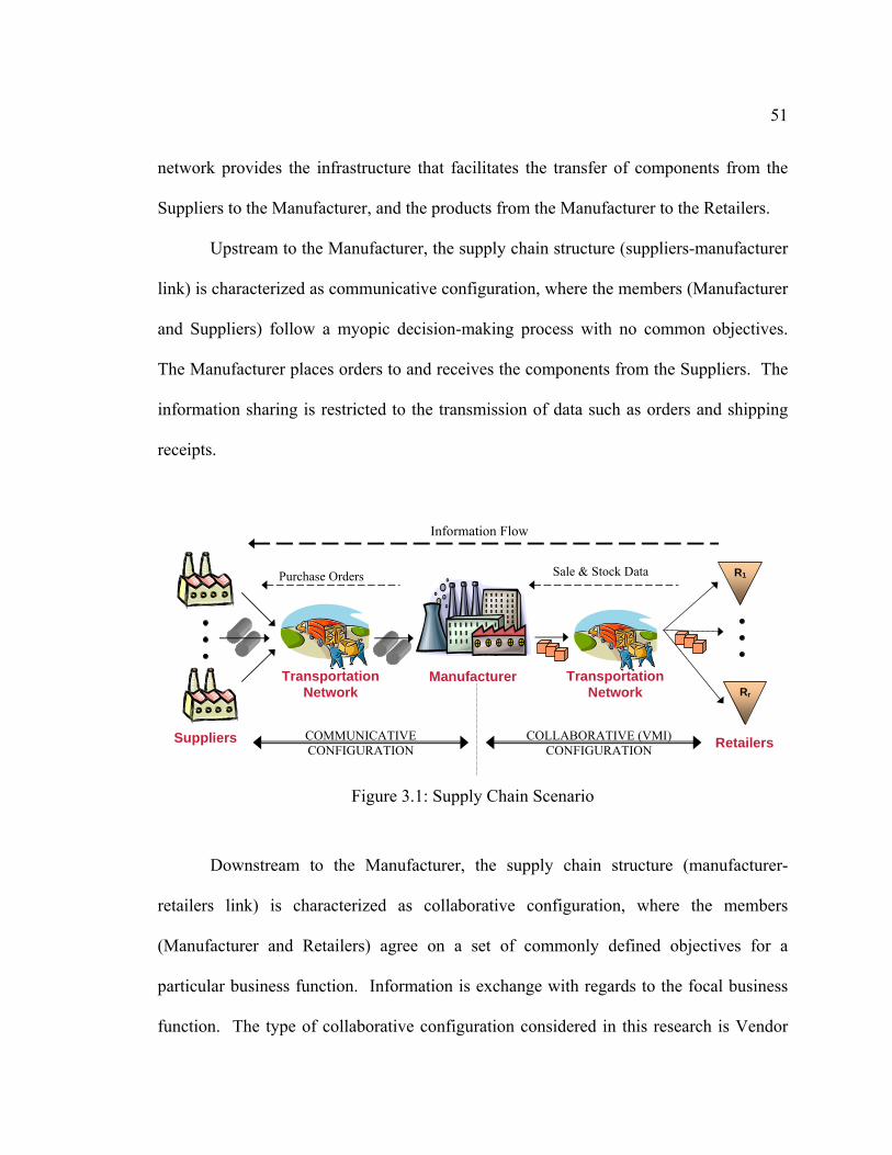
51

network provides the infrastructure that facilitates the transfer of components from the

Suppliers to the Manufacturer, and the products from the Manufacturer to the Retailers.

Upstream to the Manufacturer, the supply chain structure (suppliers-manufacturer

link) is characterized as communicative configuration, where the members (Manufacturer

and Suppliers) follow a myopic decision-making process with no common objectives.

The Manufacturer places orders to and receives the components from the Suppliers. The

information sharing is restricted to the transmission of data such as orders and shipping

receipts.

Suppliers

Manufacturer

Retailers

R1

Rr


Information Flow


Purchase Orders Sale & Stock Data


Transportation Network

Figure 3.1: Supply Chain Scenario

Downstream to the Manufacturer, the supply chain structure (manufacturer-

retailers link) is characterized as collaborative configuration, where the members

(Manufacturer and Retailers) agree on a set of commonly defined objectives for a

particular business function. Information is exchange with regards to the focal business

function. The type of collaborative configuration considered in this research is Vendor

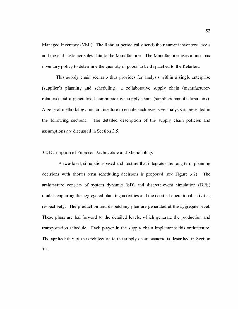
52

Managed Inventory (VMI). The Retailer periodically sends their current inventory levels

and the end customer sales data to the Manufacturer. The Manufacturer uses a min-max

inventory policy to determine the quantity of goods to be dispatched to the Retailers.

This supply chain scenario thus provides for analysis within a single enterprise

(supplier’s planning and scheduling), a collaborative supply chain (manufacturer-

retailers) and a generalized communicative supply chain (suppliers-manufacturer link).

A general methodology and architecture to enable such extensive analysis is presented in

the following sections. The detailed description of the supply chain policies and

assumptions are discussed in Section 3.5.

3.2 Description of Proposed Architecture and Methodology

A two-level, simulation-based architecture that integrates the long term planning

decisions with shorter term scheduling decisions is proposed (see Figure 3.2). The

architecture consists of system dynamic (SD) and discrete-event simulation (DES)

models capturing the aggregated planning activities and the detailed operational activities,

respectively. The production and dispatching plan are generated at the aggregate level.

These plans are fed forward to the detailed levels, which generate the production and

transportation schedule. Each player in the supply chain implements this architecture.

The applicability of the architecture to the supply chain scenario is described in Section

3.3.

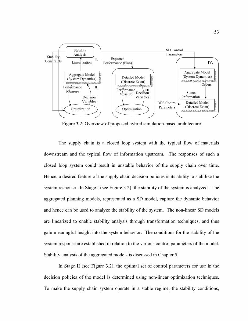
53

Aggregate Model (System Dynamics)

Optimization

Linearization

Stability Analysis

Decision Variables

Stability Constraints

Performance Measure

Detailed Model (Discrete Event)

Optimization

Decision Variables

Performance Measure

Expected Performance (Plan)

SD Control Parameters

Detailed Model (Discrete Event)

Aggregate Model (System Dynamics)

DES Control Parameters

I.

II. III.

IV.

Status Information

Orders

Figure 3.2: Overview of proposed hybrid simulation-based architecture

The supply chain is a closed loop system with the typical flow of materials

downstream and the typical flow of information upstream. The responses of such a

closed loop system could result in unstable behavior of the supply chain over time.

Hence, a desired feature of the supply chain decision policies is its ability to stabilize the

system response. In Stage I (see Figure 3.2), the stability of the system is analyzed. The

aggregated planning models, represented as a SD model, capture the dynamic behavior

and hence can be used to analyze the stability of the system. The non-linear SD models

are linearized to enable stability analysis through transformation techniques, and thus

gain meaningful insight into the system behavior. The conditions for the stability of the

system response are established in relation to the various control parameters of the model.

Stability analysis of the aggregated models is discussed in Chapter 5.

In Stage II (see Figure 3.2), the optimal set of control parameters for use in the

decision policies of the model is determined using non-linear optimization techniques.

To make the supply chain system operate in a stable regime, the stability conditions,

54

obtained through stability analysis (Stage I) are employed as additional constraints within

the optimization model. Also, the optimal production and distribution plan of the supply

chain corresponding to the optimal set of control parameters is obtained as the output.

Discussion on integrated performance and stability analysis is presented in Chapter 6.

DES models capture the detailed operational activities at the Manufacturer,

Supplier, Retailer and Transporter. In Stage III (see Figure 3.2), the optimal set of

control parameters that govern the flow of materials within the individual member units

is determined using meta-heuristic optimization techniques based on the production and

distribution plan obtained from Stage II. Section 7 describes the development of

schedules using DES models.

In Stage IV (see Figure 3.2), the optimality of the control parameters governing

the aggregated managerial policies (obtained from Stage II) and detailed operational

policies (obtained from Stage III) are concurrently evaluated using a hybrid system

dynamic and discrete-event modeling approach. In a combined SD-DES model, the

detailed operational activities (materials flows) within the supply chain are captured

using the DES models, while the management decision policies based on the aggregated

data (information flow) are captured within the SD models. The optimal control

parameters determined in Stage II and III are used in the SD and DES models,

respectively. In the SD model, the weekly production and distribution rates are converted

into daily production and distribution release quantities, and sent to the DES models. The

status of each member units, defined by the in-process and finished goods inventory and

lead time data, is feedback from the DES models to the SD models. The effects of

55

various disturbances on the local and global performances are measured in an attempt to

gain purposeful insights into the supply chain system behavior. The interaction between

SD and DES models are presented in detail in Chapter 8.

3.3 Applicability of Methodology to Supply Chain Scenario

The applicability of the proposed hybrid simulation-based architecture for the

supply chain scenario is discussed in this section.

3.3.1 Applicability to Communicative Configuration

In a communicative supply chain configuration, the supply chain members

(manufacturer-supplier) are independent and autonomous with no goal congruence or

global objective. The transactional data (purchase order) is the only data sent from the

Manufacturer to the Supplier. Now, each member, viz. the Supplier and the

Manufacturer, consists of a SD model capturing the management policies, and a DES

model capturing the operational activities. The members have their own myopic

objectives. An overview of the proposed steps involved in the methodology is as shown

in Figure 3.3. In Stage I, each member analyzes the stability of their own system using

their respective SD models. In Stage II, each member determines their own optimal set

of control parameters for use in their decision-making process captured in their respective

SD models. In Stage III, the optimal set of control parameters that govern the flow of

materials within the individual member units is determined for use in their respective

DES models, based on the plan obtained from Stage II. In the Stage IV, the optimality of

56

the control parameters obtained from Stage II and from Stage III for each member is

concurrently evaluated by interactions with the other supply chain members. The optimal

control parameters determined in Stage II and III are used in the respective SD and DES

models. The Manufacturer SD and DES models are run in synchronous with the Supplier

SD and DES models. In the SD model (Manufacturer and Suppliers), the weekly

production and distribution rates are converted into daily production and distribution

release quantities, and sent to the DES models. The status of each member units, defined

by the in-process and finished goods inventory and lead time data, is feedback from the

DES models to the SD models. The sales rate at the Supplier SD model is now

determined by the purchase orders sent from the Manufacturer SD model. The

distribution release data from the Supplier SD model are sent to the Transporter DES

model (not shown). The transporter DES model is responsible for delivery the goods to

the Manufacturer. Also, the Manufacturer DES model updates its raw material inventory

based on the component arrivals from the Supplier DES model.

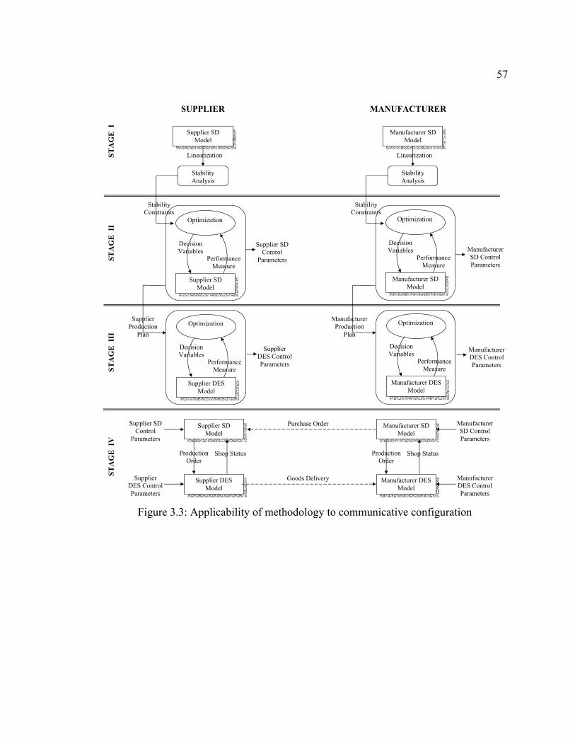
57


SUPPLIER MANUFACTURER

Supplier SD Model

STA

GE

I

Stability Analysis

Linearization

Manufacturer SD Model

Stability Analysis

Linearization

Optimization

Decision Variables

Performance Measure


Supplier SD Model

Supplier SD Control

Parameters

Supplier Production

Plan

Optimization

Decision Variables

Performance Measure


Manufacturer SD Control Parameters

Manufacturer Production

Plan

Optimization

Decision Variables

Performance Measure

Supplier DES Model

Supplier DES Control Parameters

Optimization

Decision Variables

Performance Measure

Manufacturer DES Model

Manufacturer DES Control Parameters

Production Order

Supplier SD Model

Supplier DES Model


Supplier SD Control

Parameters

Shop Status Production Order





Shop Status

Purchase Order

Goods Delivery

STA

GE

II

STA

GE

III

ST

AG

E I

V

Figure 3.3: Applicability of methodology to communicative configuration

58

3.3.2 Applicability to Collaborative Configuration

In a collaborative supply chain configuration, the supply chain members

cooperate with each other, sharing resources and capabilities, and together plan and

execute supply chain operations (Lambert et al. 1998, Simatupang and Sridharan 2002).

The supply chain members (Manufacturer and Retailers) develop a common set of

objectives for a particular business function, the popular one being the inventory function.

This is mainly to curb the increased fluctuations in inventory levels and order quantities

caused by the bullwhip effect (Lee et al. 1997). Hence, in this research vendor managed

inventory strategy is employed. Each member, viz. the Manufacturer and the Retailers,

consists of a SD model capturing the management policies, and a DES model capturing

the operational activities. An overview of the proposed steps involved is as shown in

Figure 3.4. Compared with the stages involved for communicative configuration (refer

Section 3.3.1), in collaborative configuration, the Manufacturer and Retailers interact

with each other in all Stages, I through IV. In Stage I, combined stability analysis is

performed, where the Manufacturer and Retailers’ SD models interact with each other to

capture the information exchange and their decision making interdependence. In Stage II,

the optimal set of control parameters for the Manufacturer and the Retailers, for use in

their respective the SD models are determined based on a common set of objectives, and

constrained by the stability conditions. In Stage III, the optimal set of control parameters

for the Manufacturer and Retailers, for use in the DES models are determined (based on

the plan obtained from Stage II) using on a common set of objectives. In the Stage IV,

the optimality of the control parameters obtained from Stage II and from Stage III for

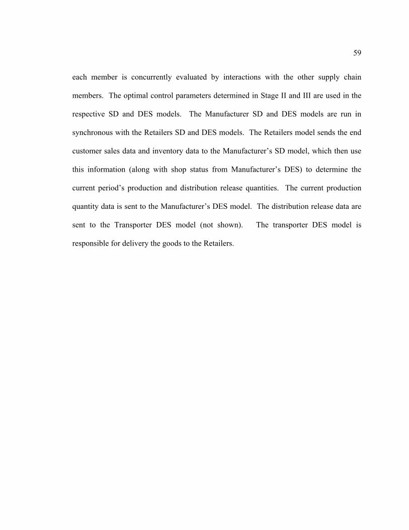
59

each member is concurrently evaluated by interactions with the other supply chain

members. The optimal control parameters determined in Stage II and III are used in the

respective SD and DES models. The Manufacturer SD and DES models are run in

synchronous with the Retailers SD and DES models. The Retailers model sends the end

customer sales data and inventory data to the Manufacturer’s SD model, which then use

this information (along with shop status from Manufacturer’s DES) to determine the

current period’s production and distribution release quantities. The current production

quantity data is sent to the Manufacturer’s DES model. The distribution release data are

sent to the Transporter DES model (not shown). The transporter DES model is

responsible for delivery the goods to the Retailers.

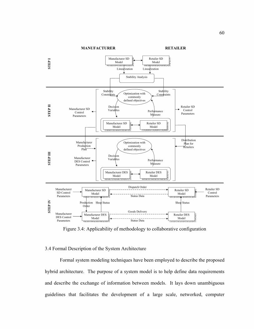
60


MANUFACTURER RETAILER


STE

P I

Stability Analysis

Linearization

Retailer SD Model

Linearization

Optimization with commonly

defined objectives

Decision Variables



Manufacturer SD Control

Parameters

Manufacturer Production

Plan

Performance Measure

Retailer SD Model

Retailer SD Control

Parameters

Distribution Plan for Retailers


Production Order





Shop Status

Retailer SD Model

Retailer DES Model

Retailer SD Control

Parameters

Shop Status

Goods Delivery

STE

P II

ST

EP

III

STE

P IV


defined objectives

Decision Variables


Performance Measure

Retailer DES Model

Status Data

Status Data

Dispatch Order

Figure 3.4: Applicability of methodology to collaborative configuration

3.4 Formal Description of the System Architecture

Formal system modeling techniques have been employed to describe the proposed

hybrid architecture. The purpose of a system model is to help define data requirements

and describe the exchange of information between models. It lays down unambiguous

guidelines that facilitates the development of a large scale, networked, computer

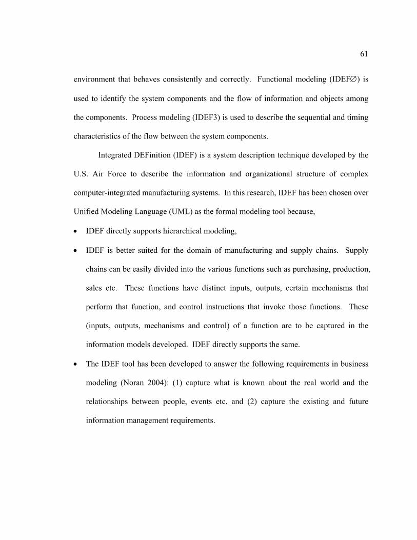
61

environment that behaves consistently and correctly. Functional modeling (IDEF∅) is

used to identify the system components and the flow of information and objects among

the components. Process modeling (IDEF3) is used to describe the sequential and timing

characteristics of the flow between the system components.

Integrated DEFinition (IDEF) is a system description technique developed by the

U.S. Air Force to describe the information and organizational structure of complex

computer-integrated manufacturing systems. In this research, IDEF has been chosen over

Unified Modeling Language (UML) as the formal modeling tool because,

• IDEF directly supports hierarchical modeling,

• IDEF is better suited for the domain of manufacturing and supply chains. Supply

chains can be easily divided into the various functions such as purchasing, production,

sales etc. These functions have distinct inputs, outputs, certain mechanisms that

perform that function, and control instructions that invoke those functions. These

(inputs, outputs, mechanisms and control) of a function are to be captured in the

information models developed. IDEF directly supports the same.

• The IDEF tool has been developed to answer the following requirements in business

modeling (Noran 2004): (1) capture what is known about the real world and the

relationships between people, events etc, and (2) capture the existing and future

information management requirements.

62

3.4.1 Functional Modeling using IDEF∅

IDEF∅ is a systematic methodology for static functional specification of the

system. The functional specification or model is a structured representation of the

functions within the system, along with the flow of information and objects which relate

the functions. In an IDEF∅ diagram the rectangular boxes represents the functions and

the arrows represent the information and object flow. Arrows entering on the left side of

the box are the inputs to the function; arrows entering the top of the box are the control

on the function; arrows entering the bottom of the box are the mechanisms that perform

the function; and the arrows leaving the box on the right side are the outputs of the

function. Each function is associated with a unique ID. Further, a function that can be

decomposed into multiple sub-functions is shown as a rectangular box-with-shadow.

The proposed hybrid architecture as applied to the supply chain scenario is

illustrated in Figure 3.5. The activities within the supply chain are segregated into the

following functions: Plan and Schedule Suppliers Production (A1), Plan and Schedule

Manufacturer’s Production (A2), Manage Retailer’s Inventory (A3), Plan and Schedule

Transportation of Goods (A4), and Retail Goods (A5). The functions A1 through A5 are

decomposed into sub-functions that correspond with Stage I-IV activities in the proposed

architecture. A1 captures the activities of the supplier that develops the production plan

(output ‘Supplier Production Planning Policy’) and schedule (output ‘Supplier Production

Scheduling Policy’) for the components. A2 captures the activities of the manufacturer

that develops the production plan (output ‘Manufacturer Production Planning Policy’)

and schedule (output ‘Manufacturer Production Scheduling Policy’) for the products. A3

63

captures the collaborative activities between the manufacturer and the retailer that

develops the distribution plan (‘Distribution Planning Policy’) for the products. A4

captures the activities of the transporter that develops the transportation plan (output

‘Transporter Planning Policy’) and schedule (output ‘Transporter Scheduling Policy’) for

the products and components. A5 captures the activities of the retailer.

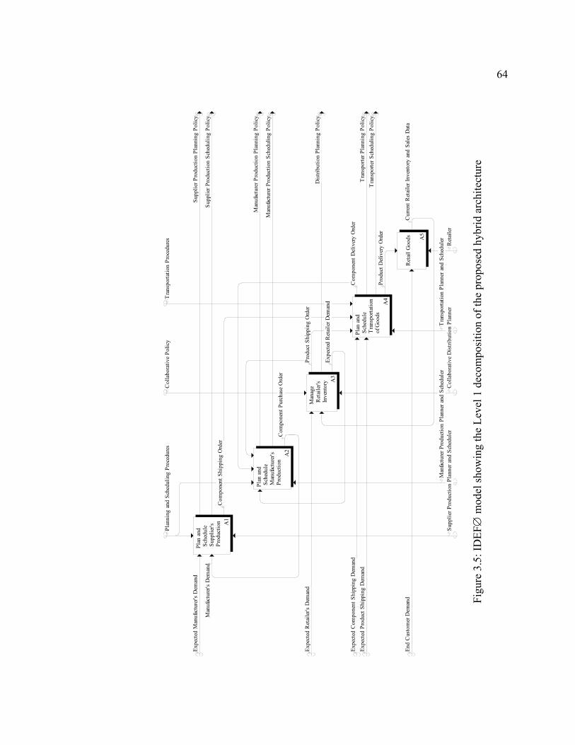
64

Ret

ail G

oods A

5

Plan

and

Sch

edul

e T

rans

porta

tion

of G

oods

A4

Man

age

Ret

aile

r's In

vent

ory A

3

Plan

and

Sch

edul

e M

anuf

actu

rer's

Pro

duct

ion

A2

Plan

and

Sch

edul

e S

uppl

ier's

Pro

duct

ion A1

End

Cus

tom

er D

eman

dC

urre

nt R

etai

ler I

nven

tory

and

Sal

es D

ata

Com

pone

nt D

eliv

ery

Ord

er

Prod

uct D

eliv

ery

Ord

er

Expe

cted

Com

pone

nt S

hipp

ing

Dem

and

Expe

cted

Pro

duct

Shi

ppin

g D

eman

dT

rans

porte

r Pla

nnin

g Po

licy

Tra

nspo

rter S

ched

ulin

g Po

licy

Expe

cted

Ret

aile

r Dem

and

Prod

uct S

hipp

ing

Ord

erEx

pect

ed R

etai

ler's

Dem

and

Dis

tribu

tion

Plan

ning

Pol

icy

Com

pone

nt P

urch

ase

Ord

er

Man

ufac

ture

r Pro

duct

ion

Plan

ning

Pol

icy

Man

ufac

ture

r Pro

duct

ion

Sche

dulin

g Po

licy

Expe

cted

Man

ufac

ture

r's D

eman

d

Com

pone

nt S

hipp

ing

Ord

er

Supp

lier P

rodu

ctio

n Pl

anni

ng P

olic

y

Supp

lier P

rodu

ctio

n Sc

hedu

ling

Polic

yM

anuf

actu

rer's

Dem

and

Ret

aile

r

Tra

nspo

rtatio

n Pr

oced

ures

Tra

nspo

rtatio

n Pl

anne

r and

Sch

edul

er

Col

labo

rativ

e Po

licy

Col

labo

rativ

e D

istri

butio

n Pl

anne

rM

anfac

ture

r Pro

duct

ion

Plan

ner a

nd S

ched

uler

Plan

ning

and

Sch

edul

ing

Proc

edur

es

Supp

lier P

rodu

ctio

n Pl

anne

r and

Sch

edul

er

Figu

re 3

.5: I

DEF

∅ m

odel

show

ing

the

Leve

l 1 d

ecom

posi

tion

of th

e pr

opos

ed h

ybrid

arc

hite

ctur

e

65

3.4.1.1 Plan and Schedule Supplier’s Production (A1)

The scope of all the functions involved in the production activities at the Supplier

is described below. The function A1 is decomposed into the sub-functions (see Figure

3.6) – Plan Supplier Production (A11) and Schedule Supplier Production (A12). A11

develops the component production plan (output ‘Supplier Production Planning Policy’)

and A12 develops the components schedule (output ‘Supplier Production Scheduling

Policy’). The functions A11 and A12 are described below:

• Plan Supplier Production (A11): Guided by the planning procedures, this function

determines the optimal expected component production release quantity, which is

sent to A12. The inputs to the function are the expected manufacturer’s demand, the

manufacturer’s demand from A2, and the current supplier shop status (WIP,

inventory and lead time) from A12. This function is further decomposed (see Figure

3.7) into Select Stable and Optimal Supplier Planning Policy (A111) and Simulate

Supplier Planning Policies (A112). Based on the expected manufacturer’s demand

input, A111 determines the optimal and stable control parameters (adjustment rates

for WIP and inventory) and the expected production release. Guided by the control

parameters, A112 determines the current production release and shipping order

quantities based on the manufacturer’s demand and the current shop status. It is

noted that function A111 corresponds with the Stage I and II activities, and the

function A112 (along with A122) corresponds with the Stage IV activities of the

Supplier in the proposed architecture.

66

• Schedule Supplier Production (A12): Guided by the scheduling procedures, this

function determines the component production quantity, which is sent to A11. The

inputs to the function are the expected production release, the current production

release and the current sales from A11, and the outputs are the current shop status

(WIP, inventory and lead time). This function is further decomposed (see Figure 3.8)

into Select Optimal Supplier Scheduling Policy (A121) and Simulate Supplier

Scheduling Policies (A122). Based on the expected production release, A121

determines the optimal queue control parameters. Guided by the queue control

parameters, A122 determines the current WIP, inventory and lead time, based on the

current component production release from A112. It is noted that function A121

corresponds with the Stage III activities and the function A122 (along with A112)

corresponds with the Stage IV activities of the Supplier in the proposed architecture.

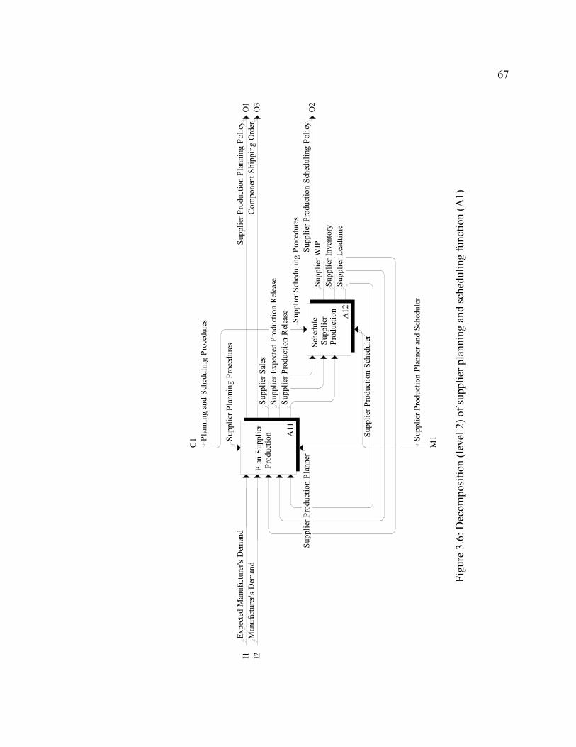
67

O2

I1 I2O

1O

3

C1

M1

Sche

dule

Sup

plie

r P

rodu

ctio

nA

12

Plan

Sup

plie

r P

rodu

ctio

n A11

Supp

lier W

IPSu

pplie

r Inv

ento

rySu

pplie

r Lea

dtim

e

Supp

lier P

rodu

ctio

n Sc

hedu

ling

Polic

y

Expe

cted

Man

ufac

ture

r's D

eman

dM

anuf

actu

rer's

Dem

and

Supp

lier E

xpec

ted

Prod

uctio

n R

elea

seSu

pplie

r Pro

duct

ion

Rel

ease

Supp

lier S

ales

Supp

lier P

rodu

ctio

n Pl

anni

ng P

olic

yC

ompo

nent

Shi

ppin

g O

rder

Supp

lier S

ched

ulin

g Pr

oced

ures

Supp

lier P

rodu

ctio

n Sc

hedu

ler

Plan

ning

and

Sch

edul

ing

Proc

edur

es

Supp

lier P

rodu

ctio

n Pl

anne

r and

Sch

edul

er

Supp

lier P

lann

ing

Proc

edur

es

Supp

lier P

rodu

ctio

n Pl

anne

r

Figu

re 3

.6: D

ecom

posi

tion

(leve

l 2) o

f sup

plie

r pla

nnin

g an

d sc

hedu

ling

func

tion

(A1)

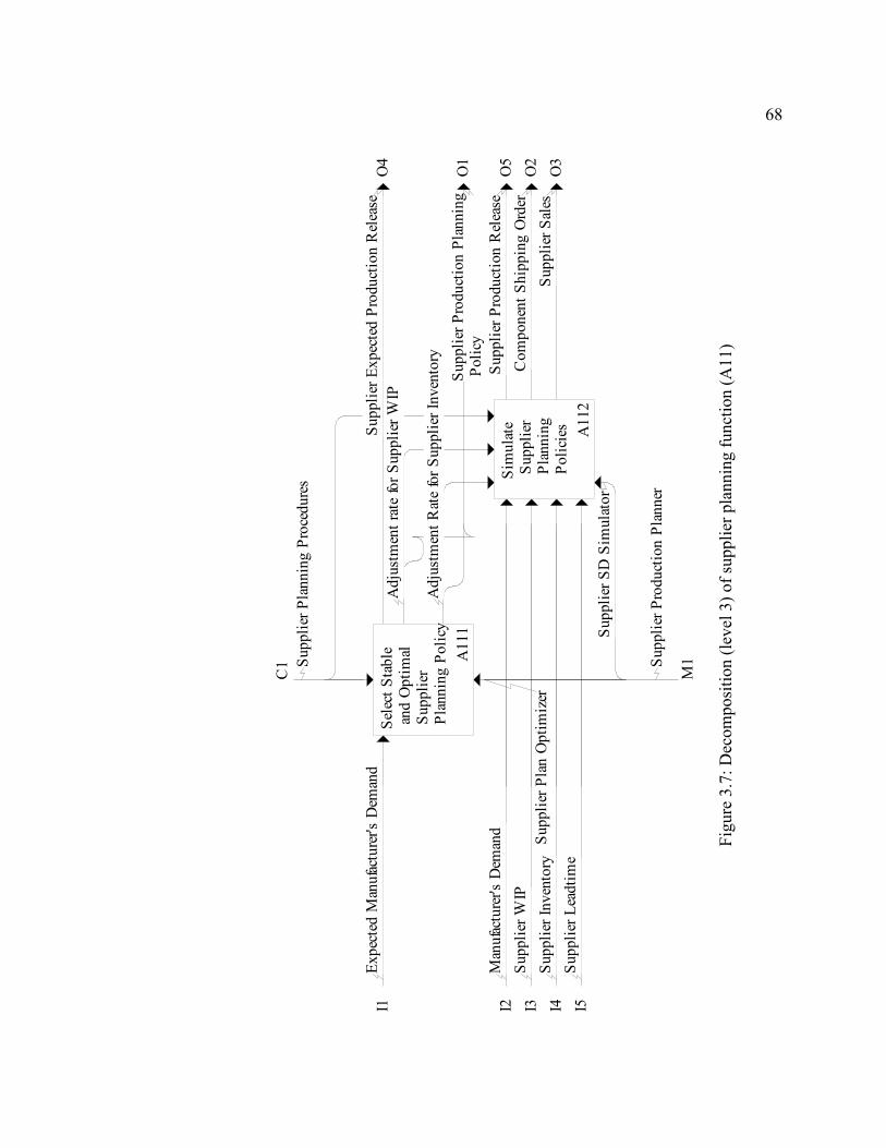
68

I2 I3 I4 I5

O5

O2

O3

I1O

4

O1

M1

C1

Sim

ulat

e S

uppl

ier

Pla

nnin

g P

olic

ies A11

2

Sele

ct S

tabl

e a

nd O

ptim

al S

uppl

ier

Pla

nnin

g Po

licy

A11

1

Man

ufac

ture

r's D

eman

dSu

pplie

r WIP

Supp

lier I

nven

tory

Supp

lier L

eadt

ime

Supp

lier P

rodu

ctio

n R

elea

seC

ompo

nent

Shi

ppin

g O

rder

Supp

lier S

ales

Expe

cted

Man

ufac

ture

r's D

eman

dA

djus

tmen

t rat

e fo

r Sup

plie

r WIP

Adj

ustm

ent R

ate

for S

uppl

ier I

nven

tory

Supp

lier E

xpec

ted

Prod

uctio

n R

elea

se

Supp

lier P

rodu

ctio

n Pl

anni

ng P

olic

y

Supp

lier S

D S

imul

ator

Supp

lier P

lann

ing

Proc

edur

es

Supp

lier P

rodu

ctio

n Pl

anne

r

Supp

lier P

lan

Opt

imiz

er

Figu

re 3

.7: D

ecom

posi

tion

(leve

l 3) o

f sup

plie

r pla

nnin

g fu

nctio

n (A

11)

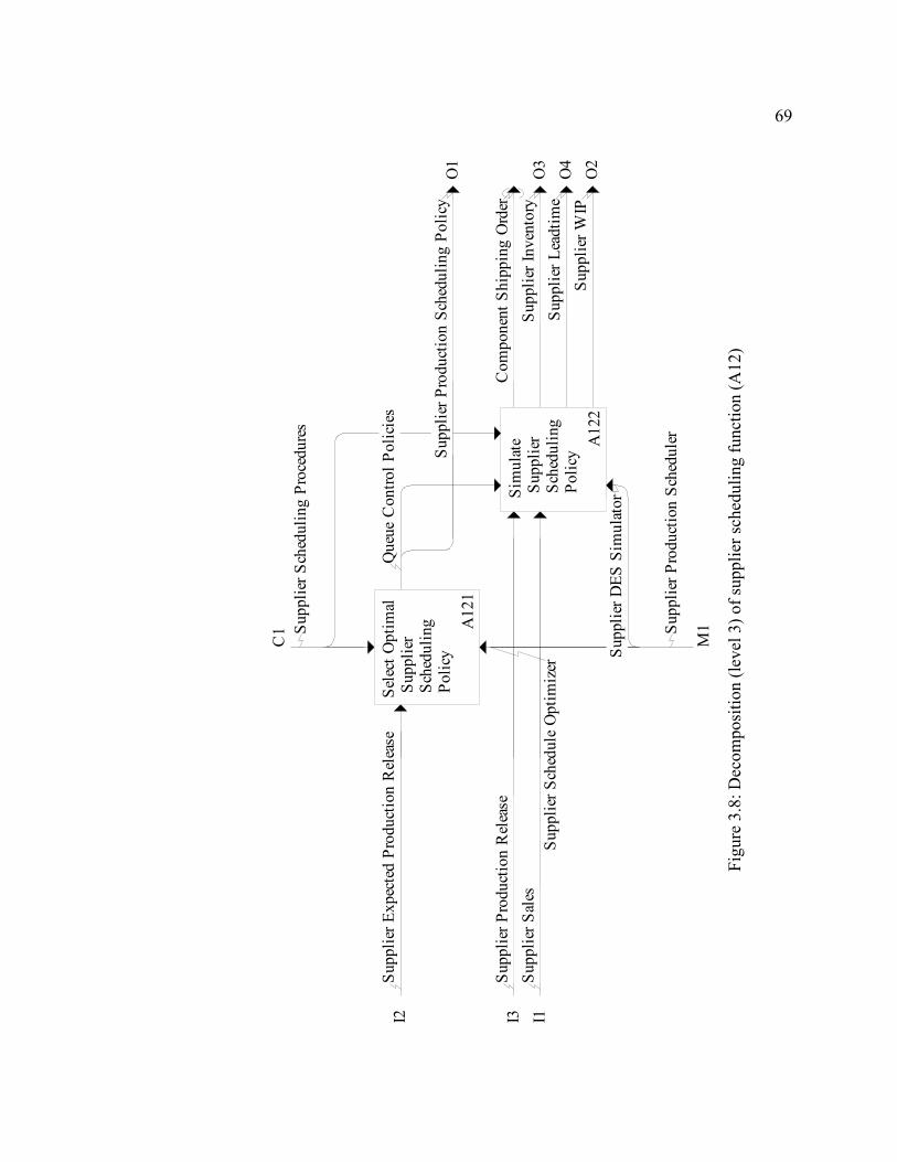
69

I3

O2

O3

O4

I1I2

O1

M1

C1

Sim

ulat

e S

uppl

ier

Sch

edul

ing

Pol

icy

A12

2

Sele

ct O

ptim

al S

uppl

ier

Sch

edul

ing

Pol

icy

A12

1

Supp

lier P

rodu

ctio

n R

elea

seSu

pplie

r Sal

esC

ompo

nent

Shi

ppin

g O

rder

Supp

lier W

IP

Supp

lier I

nven

tory

Supp

lier L

eadt

ime

Supp

lier E

xpec

ted

Prod

uctio

n R

elea

seQ

ueue

Con

trol P

olic

ies

Supp

lier P

rodu

ctio

n Sc

hedu

ling

Polic

y

Supp

lier D

ES S

imul

ator

Supp

lier S

ched

ulin

g Pr

oced

ures

Supp

lier P

rodu

ctio

n Sc

hedu

ler

Supp

lier S

ched

ule

Opt

imiz

er

Figu

re 3

.8: D

ecom

posi

tion

(leve

l 3) o

f sup

plie

r sch

edul

ing

func

tion

(A12

)

70

3.4.1.2 Plan and Schedule Manufacturer’s Production (A2)

The scope of all the functions involved in the production activities at the

Manufacturer is described below. The function A2 is decomposed into the sub-functions

(see Figure 3.9) – Plan Manufacturer Production (A21) and Schedule Manufacturer

Production (A22). A21 develops the product production plan (output ‘Manufacturer

Production Planning Policy’) and A22 develops the product production schedule (output

‘Manufacturer Production Scheduling Policy’). The functions A21 and A22 are

described below:

• Plan Manufacturer Production (A21): Guided by the planning procedures, this

function determines the optimal expected product production release quantity, which

is sent to A22. Also, the output component purchase order is sent as manufacturer’s

demand to A11. The inputs to the function are the expected retailer’s demand from

A3, and the current manufacturer’s product production status (product WIP, inventory

and lead time) and the current component supply status (component GIT, inventory

and supply lead time) from A22. This function (A21) is further decomposed (see

Figure 3.10) into Select Stable and Optimal Manufacturer Planning Policy (A211)

and Simulate Manufacturer Planning Policies (A212). Based on the expected

retailer’s demand input, A211 determines the optimal and stable product control

parameters (adjustment rates for product WIP and inventory) and the optimal and

stable component control parameters (adjustment rates for component GIT and

inventory). Guided by the product and component control parameters, A212

determines the current production release quantities based on the retailer’s demand

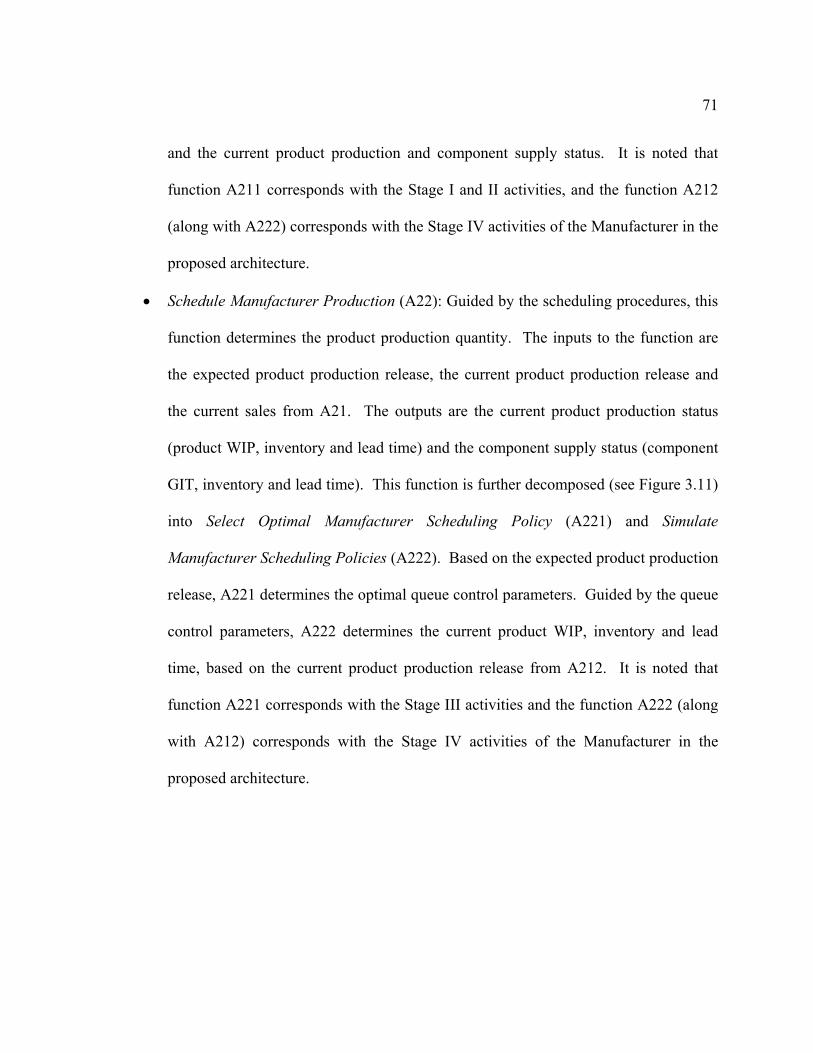
71

and the current product production and component supply status. It is noted that

function A211 corresponds with the Stage I and II activities, and the function A212

(along with A222) corresponds with the Stage IV activities of the Manufacturer in the

proposed architecture.

• Schedule Manufacturer Production (A22): Guided by the scheduling procedures, this

function determines the product production quantity. The inputs to the function are

the expected product production release, the current product production release and

the current sales from A21. The outputs are the current product production status

(product WIP, inventory and lead time) and the component supply status (component

GIT, inventory and lead time). This function is further decomposed (see Figure 3.11)

into Select Optimal Manufacturer Scheduling Policy (A221) and Simulate

Manufacturer Scheduling Policies (A222). Based on the expected product production

release, A221 determines the optimal queue control parameters. Guided by the queue

control parameters, A222 determines the current product WIP, inventory and lead

time, based on the current product production release from A212. It is noted that

function A221 corresponds with the Stage III activities and the function A222 (along

with A212) corresponds with the Stage IV activities of the Manufacturer in the

proposed architecture.

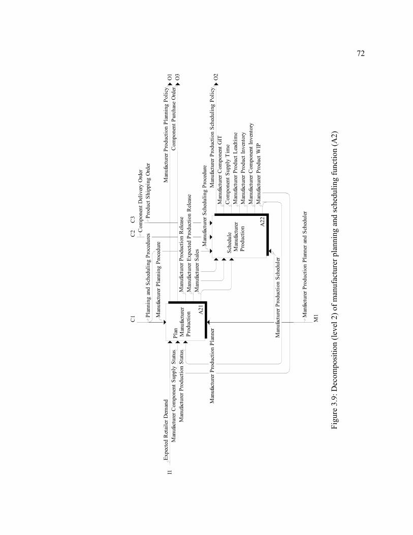
72

O2

I1O

1O

3

C2

C3

C1

M1

Sche

dule

Man

ufac

ture

r P

rodu

ctio

n A22

Plan

Man

ufac

ture

r P

rodu

ctio

n A21

Man

ufac

ture

r Pro

duct

WIP

Man

ufac

ture

r Pro

duct

Inve

ntor

yM

anuf

actu

rer P

rodu

ct L

eadt

ime

Man

ufac

ture

r Com

pone

nt G

IT

Man

ufac

ture

r Com

pone

nt In

vent

ory

Com

pone

nt S

uppl

y T

ime

Man

ufac

ture

r Pro

duct

ion

Sche

dulin

g Po

licy

Expe

cted

Ret

aile

r Dem

and

Man

ufac

ture

r Pro

duct

ion

Rel

ease

Man

ufac

ture

r Exp

ecte

d Pr

oduc

tion

Rel

ease

Man

ufac

ture

r Sal

es

Man

ufac

ture

r Pro

duct

ion

Plan

ning

Pol

icy

Com

pone

nt P

urch

ase

Ord

erM

anuf

actu

rer P

rodu

ctio

n St

atus

Man

ufac

ture

r Com

pone

nt S

uppl

y St

atus

Com

pone

nt D

eliv

ery

Ord

erPr

oduc

t Shi

ppin

g O

rder

Man

ufac

ture

r Sch

edul

ing

Proc

edur

e

Man

ufac

ture

r Pro

duct

ion

Sche

dule

r

Plan

ning

and

Sch

edul

ing

Proc

edur

es

Man

factu

rer P

rodu

ctio

n Pl

anne

r and

Sch

edul

er

Man

ufac

ture

r Pla

nnin

g Pr

oced

ure

Man

ufac

ture

r Pro

duct

ion

Plan

ner

Figu

re 3

.9: D

ecom

posi

tion

(leve

l 2) o

f man

ufac

ture

r pla

nnin

g an

d sc

hedu

ling

func

tion

(A2)

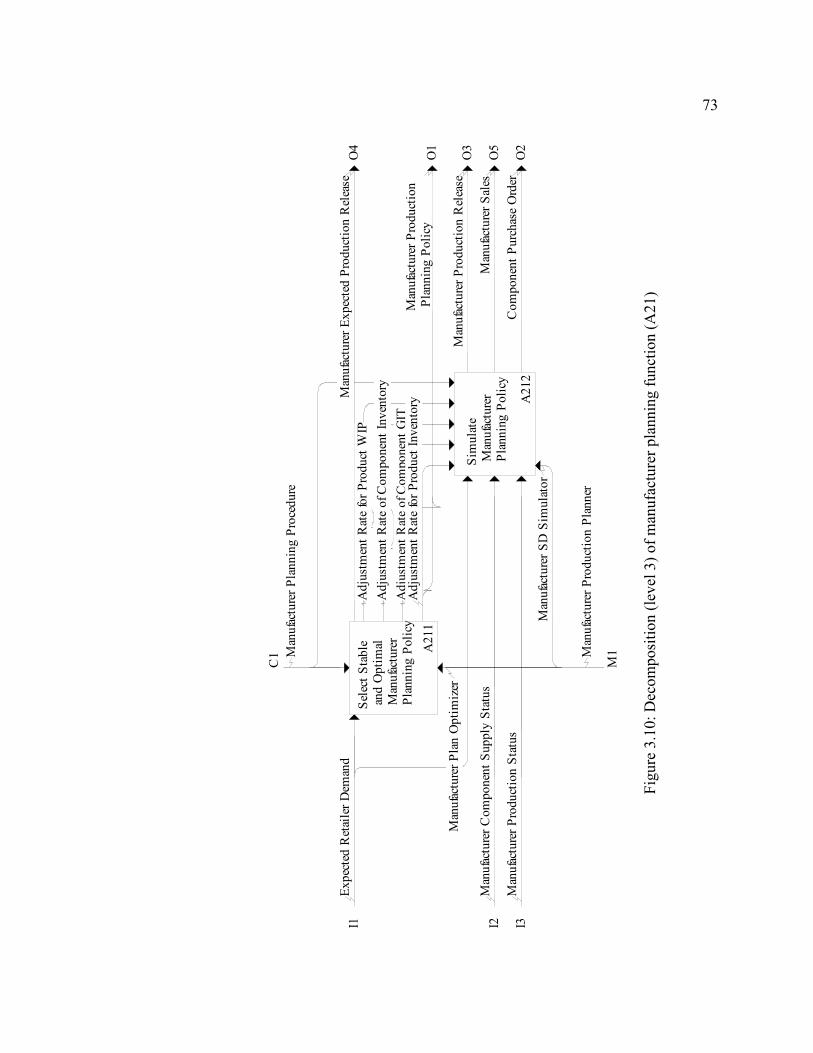
73

I2 I3O

2

O3

O5

O4

O1

M1

C1

I1

Sim

ulat

e M

anuf

actu

rer

Pla

nnin

g Po

licy

A21

2

Sele

ct S

tabl

e a

nd O

ptim

al M

anuf

actu

rer

Pla

nnin

g Po

licy

A21

1

Man

ufac

ture

r Com

pone

nt S

uppl

y St

atus

Man

ufac

ture

r Pro

duct

ion

Stat

usC

ompo

nent

Pur

chas

e O

rder

Man

ufac

ture

r Pro

duct

ion

Rel

ease

Man

ufac

ture

r Sal

es

Expe

cted

Ret

aile

r Dem

and

Adj

ustm

ent R

ate

of C

ompo

nent

GIT

Adj

ustm

ent R

ate

of C

ompo

nent

Inve

ntor

yA

djus

tmen

t Rat

e fo

r Pro

duct

WIP

Adj

ustm

ent R

ate

for P

rodu

ct In

vent

oryM

anuf

actu

rer E

xpec

ted

Prod

uctio

n R

elea

se

Man

ufac

ture

r Pro

duct

ion

Pla

nnin

g Po

licy

Man

ufac

ture

r SD

Sim

ulat

or

Man

ufac

ture

r Pla

nnin

g Pr

oced

ure

Man

ufac

ture

r Pro

duct

ion

Plan

ner

Man

ufac

ture

r Pla

n O

ptim

izer

Figu

re 3

.10:

Dec

ompo

sitio

n (le

vel 3

) of m

anuf

actu

rer p

lann

ing

func

tion

(A21

)

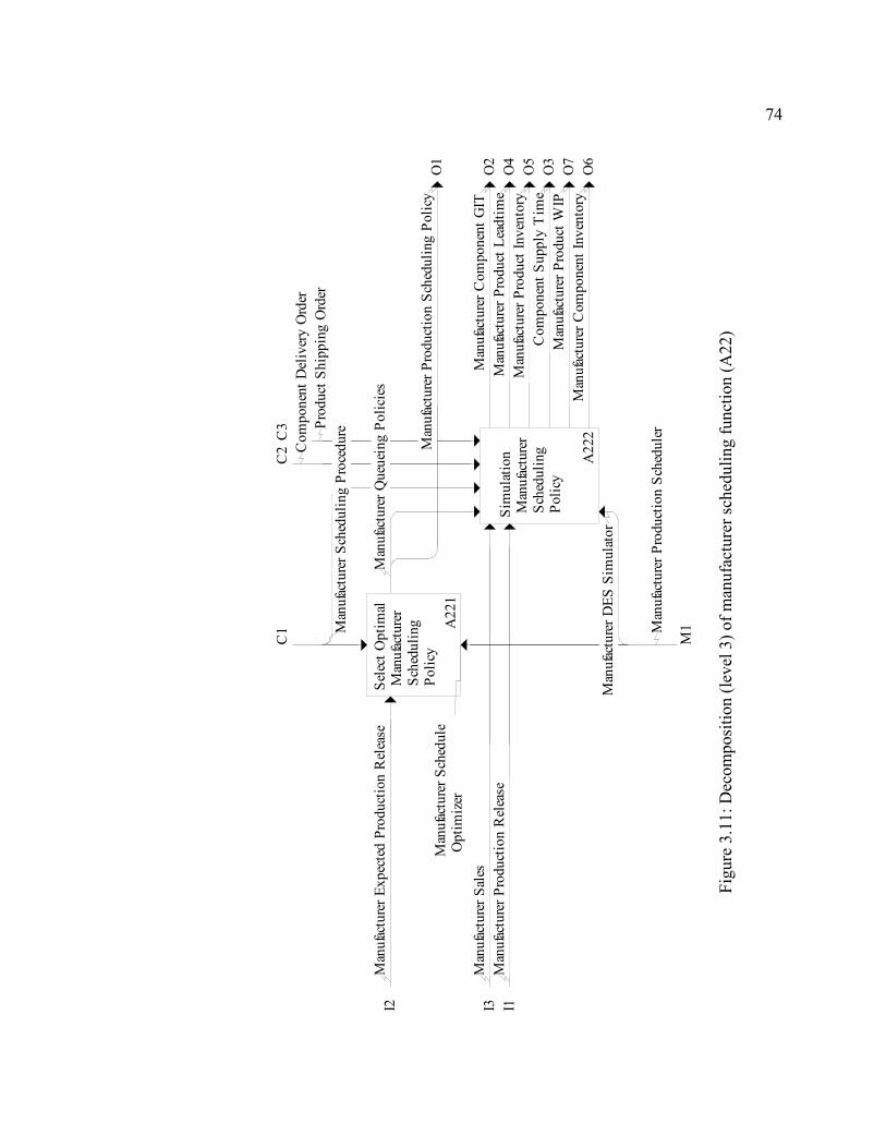
74

I1I3O

2

O3

O4

O5

O6

O7

I2

O1

C2

C3

M1

C1

Sim

ulat

ion

Man

ufac

ture

r S

ched

ulin

g P

olic

y

A22

2

Sele

ct O

ptim

al M

anuf

actu

rer

Sch

edul

ing

Pol

icy

A22

1

Man

ufac

ture

r Pro

duct

ion

Rel

ease

Man

ufac

ture

r Sal

esM

anuf

actu

rer C

ompo

nent

GIT

Com

pone

nt S

uppl

y T

ime

Man

ufac

ture

r Pro

duct

Lea

dtim

eM

anuf

actu

rer P

rodu

ct In

vent

ory

Man

ufac

ture

r Com

pone

nt In

vent

ory

Man

ufac

ture

r Pro

duct

WIP

Man

ufac

ture

r Exp

ecte

d Pr

oduc

tion

Rel

ease

Man

ufac

ture

r Que

uein

g Po

licie

s

Man

ufac

ture

r Pro

duct

ion

Sche

dulin

g Po

licy

Com

pone

nt D

eliv

ery

Ord

erPr

oduc

t Shi

ppin

g O

rder

Man

ufac

ture

r DES

Sim

ulat

or

Man

ufac

ture

r Sch

edul

ing

Proc

edur

e

Man

ufac

ture

r Pro

duct

ion

Sche

dule

r

Man

ufac

ture

r Sch

edul

e O

ptim

izer

Figu

re 3

.11:

Dec

ompo

sitio

n (le

vel 3

) of m

anuf

actu

rer s

ched

ulin

g fu

nctio

n (A

22)

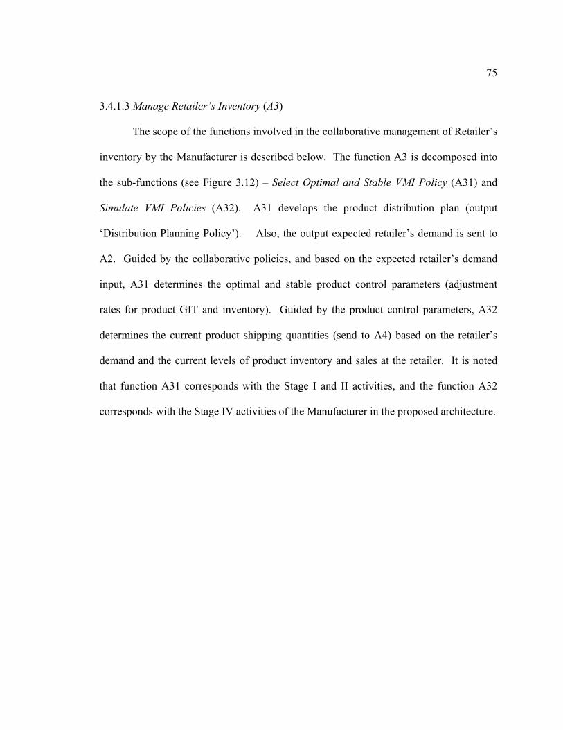
75

3.4.1.3 Manage Retailer’s Inventory (A3)

The scope of the functions involved in the collaborative management of Retailer’s

inventory by the Manufacturer is described below. The function A3 is decomposed into

the sub-functions (see Figure 3.12) – Select Optimal and Stable VMI Policy (A31) and

Simulate VMI Policies (A32). A31 develops the product distribution plan (output

‘Distribution Planning Policy’). Also, the output expected retailer’s demand is sent to

A2. Guided by the collaborative policies, and based on the expected retailer’s demand

input, A31 determines the optimal and stable product control parameters (adjustment

rates for product GIT and inventory). Guided by the product control parameters, A32

determines the current product shipping quantities (send to A4) based on the retailer’s

demand and the current levels of product inventory and sales at the retailer. It is noted

that function A31 corresponds with the Stage I and II activities, and the function A32

corresponds with the Stage IV activities of the Manufacturer in the proposed architecture.

76

I2O

1

O3

I1

O2

M1

C1

Sim

ulat

e V

MI

Pol

icie

s

A32

Sele

ct O

ptim

al a

nd S

tabl

e V

MI

pol

icy

A31

Cur

rent

Ret

aile

r Inv

ento

ry a

nd S

ales

Dat

aPr

oduc

t Shi

ppin

g O

rder

Expe

cted

Ret

aile

r's D

eman

dA

djus

tmen

t Rat

e fo

r Pro

duct

GIT

Adj

ustm

ent R

ate

for R

etai

ler I

nven

tory

Expe

cted

Ret

aile

r Dem

and

Dis

tribu

tion

Plan

ning

Pol

icy

VM

I SD

Sim

ulat

or

Col

labo

rativ

e Po

licy

Col

labo

rativ

e D

istri

butio

n Pl

anne

r

VM

I Pla

n O

ptim

izer

Figu

re 3

.12:

Dec

ompo

sitio

n (le

vel 2

) of r

etai

ler’

s inv

ento

ry m

anag

emen

t (A

3)

77

3.4.1.4 Plan and Schedule Transportation of Goods (A4)

The scope of all the functions involved in the transport activities at the

Transporter is described below. The function A4 is decomposed into the sub-functions

(see Figure 3.13) – Plan Transportation (A41) and Schedule Transportation (A42). A41

develops the product and component transportation plan (output ‘Transportation Planning

Policy’) and A42 develops the product and component transportation schedule (output

‘Transportation Scheduling Policy’). The functions A41 and A42 are described below:

• Plan Transportation (A41): Guided by the transportation procedures, this function

determines the optimal expected product dispatch quantities and component dispatch

quantities, which is sent to A42. The inputs to the function are the expected

component shipping demand and expected product shipping demand, and the current

transportation status (component and product goods-in-shipment and transport lead

times) from A42. This function (A41) is further decomposed (see Figure 3.14) into

Select Stable and Optimal Transportation Planning Policy (A411) and Simulate

Transportation Planning Policies (A412). Based on the expected product and

component demand inputs, A411 determines the optimal and stable product transport

control parameters (adjustment rates for product goods-in-shipment and goods-

awaiting-shipment) and the optimal and stable component transport control

parameters (adjustment rates for product goods-in-shipment and goods-awaiting-

shipment). Guided by the product and component control parameters, A412

determines the current transport quantities based on the shipping demand and the

78

current product and component transport status. It is noted that function A411

corresponds with the Stage I and II activities, and the function A412 (along with

A422) corresponds with the Stage IV activities of the Transporter in the proposed

architecture.

• Schedule Transportation (A42): Guided by the transportation procedures, this

function determines the product and component transportation quantities. The inputs

to the function are the expected product and component dispatches from A41. The

outputs are the current product transport status (product goods-in-shipment and lead

time) and the component transport status (component goods-in-shipment, and

transport lead time). This function is further decomposed (see Figure 3.15) into

Select Optimal Transportation Scheduling Policy (A421) and Simulate

Transportation Scheduling Policies (A422). Based on the expected product and

component transportation quantities, A421 determines the optimal transportation

routing control parameters. Guided by the routing control parameters, A422

determines the current product and component goods-in-shipment, based on the

current product and component dispatches A412. It is noted that function A421

corresponds with the Stage III activities and the function A422 (along with A412)

corresponds with the Stage IV activities of the Transporter in the proposed

architecture.

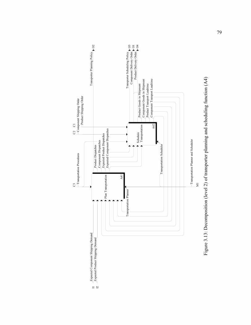
79

O3

O2

I1 I2

C1

C2

M1

C3

O1

O4

Sche

dule

Tra

nspo

rtatio

n

A42

Plan

Tra

nspo

rtatio

n

A41

Com

pone

nt G

oods

in S

hipm

ent

Prod

uct G

oods

in S

hipm

ent

Prod

uct T

rans

port

Lead

time

Com

pone

nt T

rans

port

Lead

time

Com

pone

nt D

eliv

ery

Ord

erPr

oduc

t Del

iver

y O

rder

Tra

nspo

rter S

ched

ulin

g Po

licy

Com

pone

nt D

ispa

tche

sPr

oduc

t Dis

patc

hes

Expe

cted

Com

pone

nt S

hipp

ing

Dem

and

Expe

cted

Pro

duct

Shi

ppin

g D

eman

d

Expe

cted

Com

pone

nt D

ispa

tche

sEx

pect

ed P

rodu

ct D

ispa

tche

s

Tra

nspo

rter P

lann

ing

Polic

y

Prod

uct S

hipp

ing

Ord

erC

ompo

nent

Shi

ppin

g O

rder

Tra

nspo

rtatio

n Sc

hedu

ler

Tra

nspo

rtatio

n Pr

oced

ures

Tra

nspo

rtatio

n Pl

anne

r and

Sch

edul

er

Tra

nspo

rtatio

n Pl

anne

r

Figu

re 3

.13:

Dec

ompo

sitio

n (le

vel 2

) of t

rans

porte

r pla

nnin

g an

d sc

hedu

ling

func

tion

(A4)

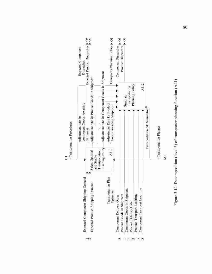
80

I3 I4I5 I6O

2O

3

I7 I8I1 I2O

4O

5

O1

M1

C1

Sim

ulat

e T

rans

porta

tion

Pla

nnin

g Po

licy

A41

2

Sele

ct O

ptim

al a

nd S

tabl

e T

rans

porta

tion

Pla

nnin

g Po

licy

A41

1

Com

pone

nt D

eliv

ery

Ord

er

Prod

uct D

eliv

ery

Ord

er

Prod

uct G

oods

in S

hipm

ent

Com

pone

nt G

oods

in S

hipm

ent

Prod

uct T

rans

port

Lead

time

Com

pone

nt T

rans

port

Lead

time

Prod

uct D

ispa

tche

sC

ompo

nent

Dis

patc

hes

Expe

cted

Com

pone

nt S

hipp

ing

Dem

and

Expe

cted

Pro

duct

Shi

ppin

g D

eman

d

Adj

ustm

ent r

ate

for C

ompo

nent

Goo

ds in

Shi

pmen

t

Adj

ustm

ent r

ate

for P

rodu

ct G

oods

in S

hipm

ent

Adj

sutm

ent r

ate

for

com

pone

nt G

oods

Aw

aitin

g S

hipm

ent

Adj

sutm

ent R

ate

for P

rodu

ct G

oods

Aw

aitin

g Sh

ipm

ent

Expe

cted

Pro

duct

Dis

patc

hes

Expe

cted

Com

pone

nt D

ispa

tche

s

Tra

nspo

rter P

lann

ing

Polic

y

Tra

nspo

rtatio

n SD

Sim

ulat

or

Tra

nspo

rtatio

n Pr

oced

ures

Tra

nspo

rtatio

n Pl

anne

r

Tra

nspo

rtatio

n Pl

an O

ptim

izer

Figu

re 3

.14:

Dec

ompo

sitio

n (le

vel 3

) of t

rans

porte

r pla

nnin

g fu

nctio

n (A

41)

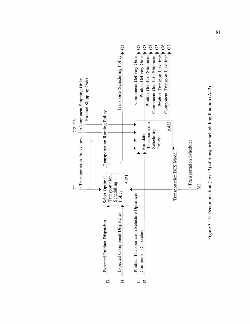
81

I1 I2O

2O

3O

4O

5O

6O

7

I3 I4O

1

C2

C3

M1

C1

Sim

ulat

e T

rans

porta

tion

Sch

edul

ing

Pol

icy

A42

2

Sele

ct O

ptim

al T

rans

porta

tion

Sch

edul

ing

Pol

icy

A42

1

Prod

uct D

ispa

tche

sC

ompo

nent

Dis

patc

hes

Com

pone

nt D

eliv

ery

Ord

erPr

oduc

t Del

iver

y O

rder

Prod

uct G

oods

in S

hipm

ent

Com

pone

nt G

oods

in S

hipm

ent

Prod

uct T

rans

port

Lead

time

Com

pone

nt T

rans

port

Lead

time

Expe

cted

Pro

duct

Dis

patc

hes

Expe

cted

Com

pone

nt D

ispa

tche

s

Tra

nspo

rtatio

n R

outin

g Po

licy T

rans

porte

r Sch

edul

ing

Polic

y

Com

pone

nt S

hipp

ing

Ord

erPr

oduc

t Shi

ppin

g O

rder

Tra

nspo

rtatio

n D

ES M

odel

Tra

nspo

rtatio

n Pr

oced

ures

Tra

nspo

rtatio

n Sc

hedu

ler

Tra

nspo

rtatio

n Sc

hedu

le O

ptim

izer

Figu

re 3

.15:

Dec

ompo

sitio

n (le

vel 3

) of t

rans

porte

r sch

edul

ing

func

tion

(A42

)

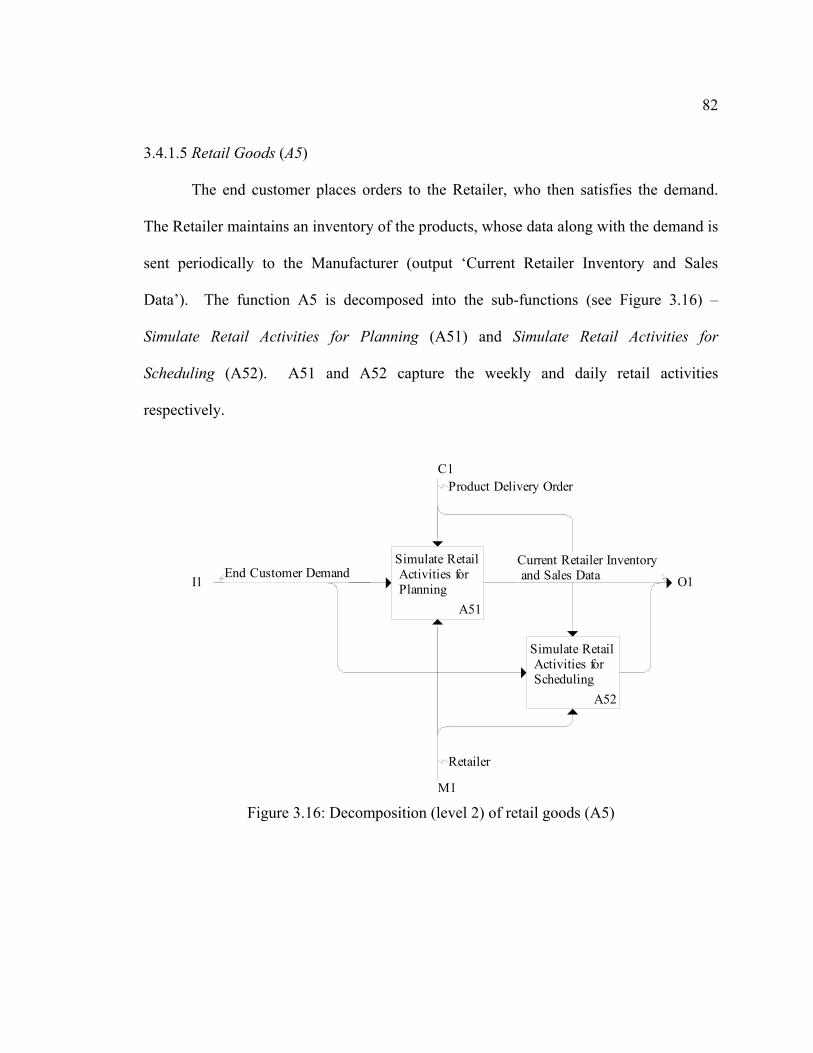
82

3.4.1.5 Retail Goods (A5)

The end customer places orders to the Retailer, who then satisfies the demand.

The Retailer maintains an inventory of the products, whose data along with the demand is

sent periodically to the Manufacturer (output ‘Current Retailer Inventory and Sales

Data’). The function A5 is decomposed into the sub-functions (see Figure 3.16) –

Simulate Retail Activities for Planning (A51) and Simulate Retail Activities for

Scheduling (A52). A51 and A52 capture the weekly and daily retail activities

respectively.

O1

C1

M1

I1

Simulate Retail Activities for Scheduling

A52

Simulate Retail Activities for Planning

A51

End Customer DemandCurrent Retailer Inventory and Sales Data

Product Delivery Order

Retailer

Figure 3.16: Decomposition (level 2) of retail goods (A5)

83

3.4.2 Process Modeling using IDEF3

As shown in the previous section, the IDEF∅ presents a static model of the

system; hence there is no guarantee that the functions will follow the sequence outlined in

the diagrams. IDEF3 helps capture the precedence and causality relation between the

various processes in the system. A process (called as Unit of Behavior) is shown as a

rectangular box with three compartments. The process represents different types of

behavior such as operations, decisions, function or events that occur in the system. The

processes are linked together to form a process path. The timing and sequencing

characteristics of the process paths are defined using logical connectors such as XOR (X),

AND (&) and OR (O). The IDEF3 processes are mapped with the IDEF∅ functions

using the function ID. All the process contains the ID of the function it is associated with

in its right bottom compartment. The left bottom compartment contains the process ID

unique to the described scenario.

The sequence of interactions among the processes involved in the Stage I, II and

III activities of the Supplier functions A111 and A121 is illustrated in Figure 3.17. The

processes ‘Determine Stable Planning Policy’, ‘Determine Optimal Planning Policy’,

‘Calculate Expected Production Release’ and ‘Update Adjustment Rates for WIP and

Inventory’ are associated with the IDEFØ function Select Stable and Optimal

Manufacturer Planning Policy (A111). The processes ‘Determine Optimal Scheduling

Policy’ and ‘Update Queues Control Policies’ are associated with the IDEFØ function

Select Optimal Manufacturer Scheduling Policy (A121). The process begins with the

determination of the stability conditions for the various control parameters that are then

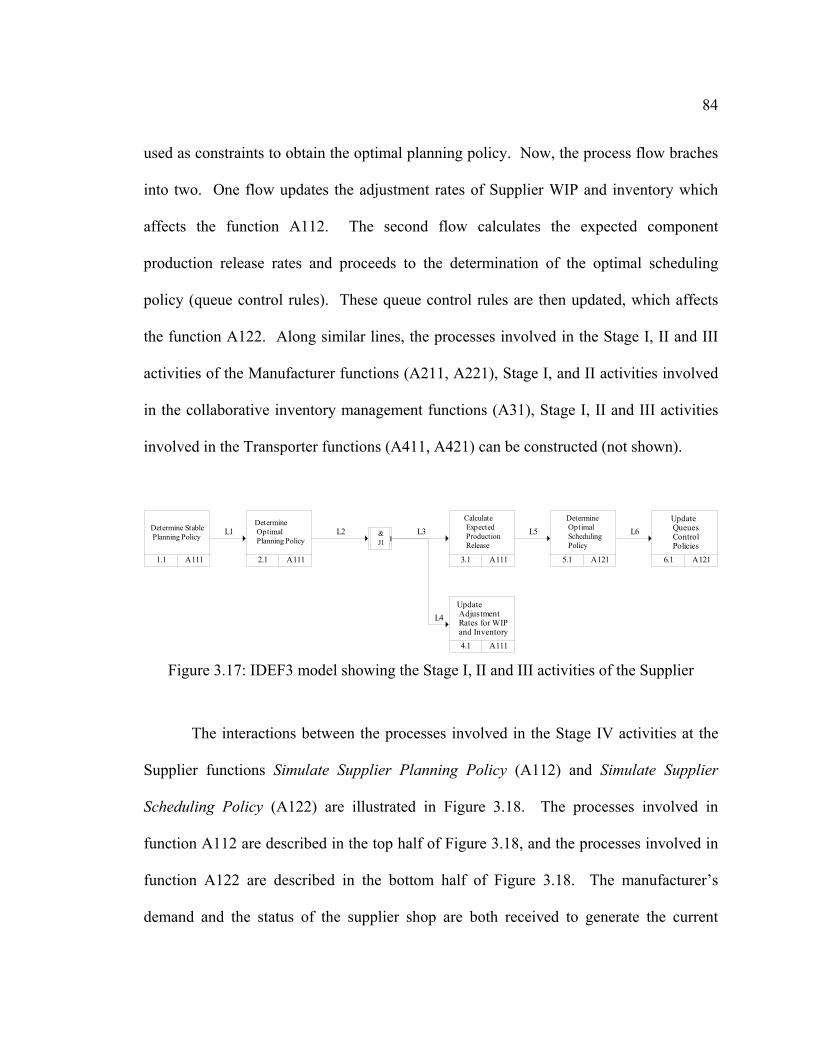
84

used as constraints to obtain the optimal planning policy. Now, the process flow braches

into two. One flow updates the adjustment rates of Supplier WIP and inventory which

affects the function A112. The second flow calculates the expected component

production release rates and proceeds to the determination of the optimal scheduling

policy (queue control rules). These queue control rules are then updated, which affects

the function A122. Along similar lines, the processes involved in the Stage I, II and III

activities of the Manufacturer functions (A211, A221), Stage I, and II activities involved

in the collaborative inventory management functions (A31), Stage I, II and III activities

involved in the Transporter functions (A411, A421) can be constructed (not shown).

Update Queues Control Policies

6.1 A121

Determine Optimal Scheduling Policy

5.1 A121

Update Adjustment Rates for WIP and Inventory4.1 A111

Calculate Expected Production Release

3.1 A111

&J1

Determine Optimal Planning Policy

2.1 A111

Determine Stable Planning Policy

1.1 A111

L6L5

L4

L3L2L1

Figure 3.17: IDEF3 model showing the Stage I, II and III activities of the Supplier

The interactions between the processes involved in the Stage IV activities at the

Supplier functions Simulate Supplier Planning Policy (A112) and Simulate Supplier

Scheduling Policy (A122) are illustrated in Figure 3.18. The processes involved in

function A112 are described in the top half of Figure 3.18, and the processes involved in

function A122 are described in the bottom half of Figure 3.18. The manufacturer’s

demand and the status of the supplier shop are both received to generate the current

85

component production release order and the component shipping order. The object

‘Adjustment Rates for Supplier WIP and Inventory’ is referred to in the process of

component production release order generation. It is noted that this object is updated by

the ‘Update Adjustment Rates for WIP and Inventory’ process (see Figure 3.17). An

object is represented as a two-compartment box, without any process ID, and association

to any particular process shown by solid line links. The component shipping order is sent

to the function A42. The component production release order is sent to the Supplier shop.

Once the order is received by the shop, the corresponding entities are release to the shop.

The production process is continued, governed by the object ‘Supplier’s Queues Control

Policies’. At the end of the sampling interval, the current values of WIP, inventory and

lead time are obtained and sent to the function A112.

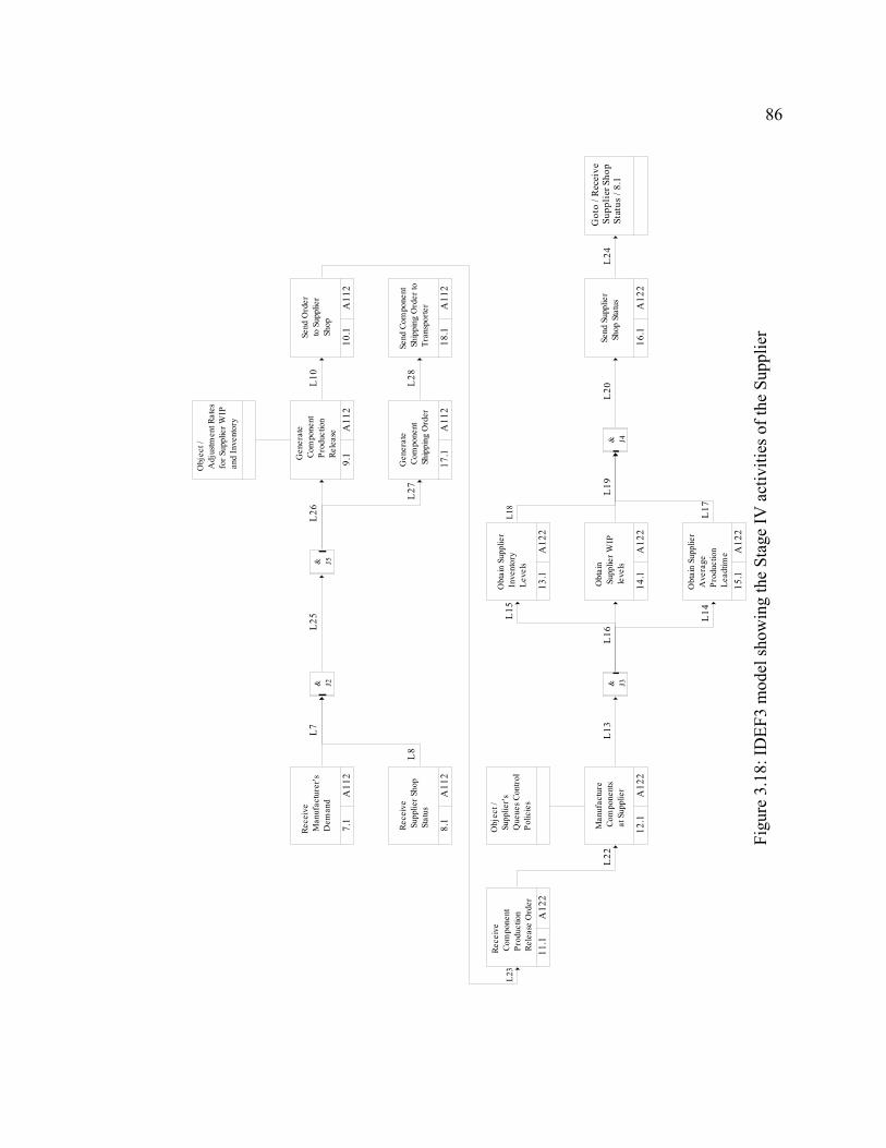
86

Got

o / R

ecei

ve S

uppl

ier S

hop

Sta

tus

/ 8.1

Send

Sup

plie

r S

hop

Stat

us

16.1

A12

2

& J4

Obt

ain

Sup

plie

r WIP

leve

ls

14.1

A12

2

Obt

ain

Supp

lier

Inve

ntor

y L

evel

s

13.1

A12

2

Obt

ain

Supp

lier

Ave

rage

Pro

duct

ion

Lea

dtim

e15

.1A

122

& J3

Man

ufac

ture

Com

pone

nts

at S

uppl

ier

12.1

A12

2

Rece

ive

Com

pone

nt P

rodu

ctio

n R

elea

se O

rder

11.1

A12

2

Send

Ord

er to

Sup

plie

r S

hop

10.1

A11

2

Send

Com

pone

nt S

hipp

ing

Ord

er to

Tra

nspo

rter

18.1

A11

2

Gen

erat

e C

ompo

nent

Shi

ppin

g O

rder

17.1

A11

2

Gen

erat

e C

ompo

nent

Pro

duct

ion

Rel

ease

9.1

A11

2

& J5& J2

Rece

ive

Man

ufac

ture

r's D

eman

d

7.1

A11

2

Rece

ive

Sup

plie

r Sho

p S

tatu

s

8.1

A11

2

L8

L17

L18

L24

L20

L19

L16

L15

L14

L13

L22

L23

L10

L28

L27

L26

L25

L7

Obj

ect /

Sup

plie

r's Q

ueue

s Con

trol

Pol

icie

s

Obj

ect /

Adj

ustm

ent R

ates

for S

uppl

ier W

IP a

nd In

vent

ory

Figu

re 3

.18:

IDEF

3 m

odel

show

ing

the

Stag

e IV

act

iviti

es o

f the

Sup

plie

r

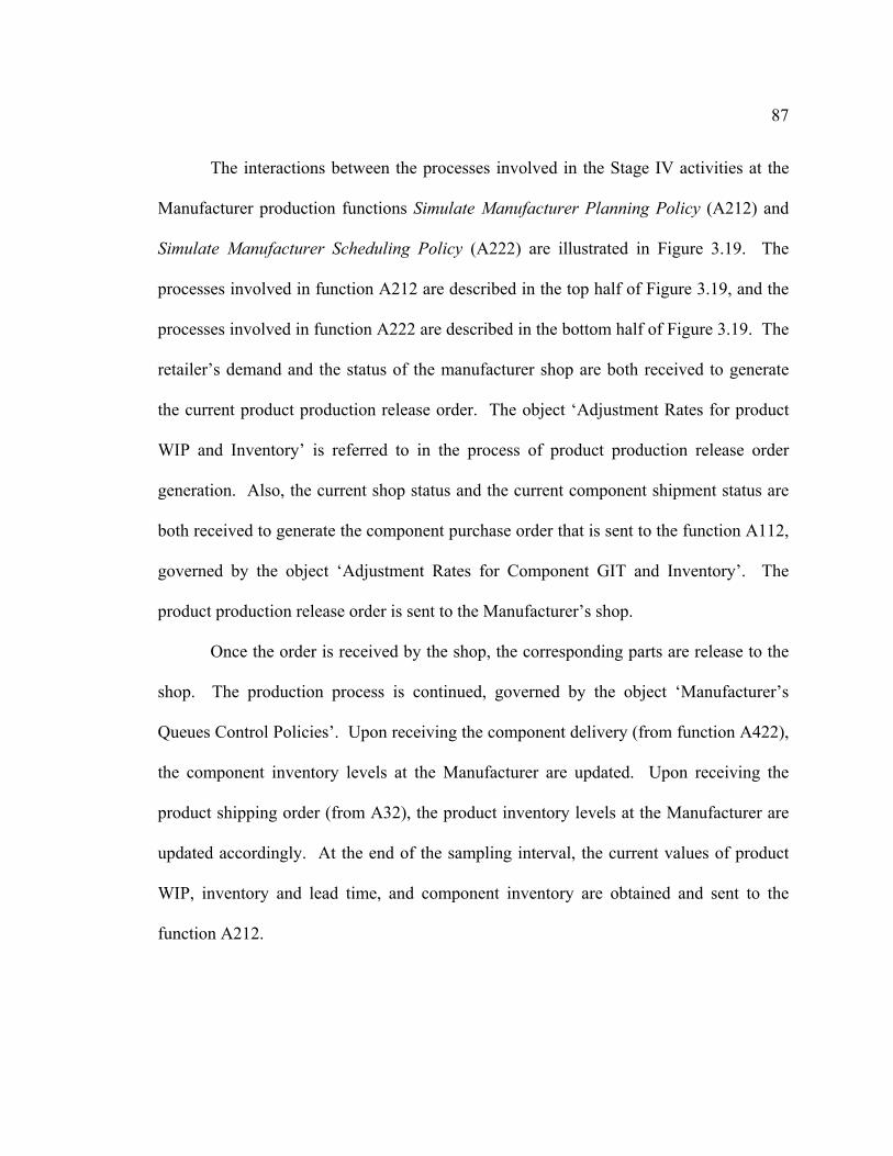
87


Manufacturer production functions Simulate Manufacturer Planning Policy (A212) and

Simulate Manufacturer Scheduling Policy (A222) are illustrated in Figure 3.19. The

processes involved in function A212 are described in the top half of Figure 3.19, and the

processes involved in function A222 are described in the bottom half of Figure 3.19. The

retailer’s demand and the status of the manufacturer shop are both received to generate

the current product production release order. The object ‘Adjustment Rates for product

WIP and Inventory’ is referred to in the process of product production release order

generation. Also, the current shop status and the current component shipment status are

both received to generate the component purchase order that is sent to the function A112,

governed by the object ‘Adjustment Rates for Component GIT and Inventory’. The

product production release order is sent to the Manufacturer’s shop.

Once the order is received by the shop, the corresponding parts are release to the

shop. The production process is continued, governed by the object ‘Manufacturer’s

Queues Control Policies’. Upon receiving the component delivery (from function A422),

the component inventory levels at the Manufacturer are updated. Upon receiving the

product shipping order (from A32), the product inventory levels at the Manufacturer are

updated accordingly. At the end of the sampling interval, the current values of product

WIP, inventory and lead time, and component inventory are obtained and sent to the

function A212.

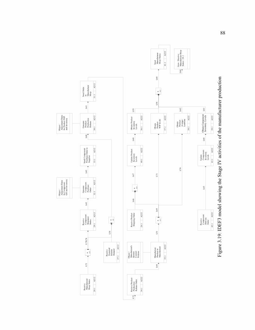
88

Obt

ain

Com

pone

nt In

vent

ory

Leve

ls

39.1

A22

2

Upd

ate

Com

pone

nt In

vent

ory

Lev

els

43.1

A22

2

Send

Com

pone

nt P

urch

ase

Ord

er to

Sup

plie

r

33.1

A21

2

Gen

erat

e C

ompo

nent

Pur

chas

e O

rder

32.1

A21

2

Rec

eive

Com

pone

nt S

hipm

ent

Sta

tus

29.1

A21

2

& J15

Obt

ain

Prod

uct

Inve

ntor

y L

evel

s

36.1

A22

2

Upd

ate

Prod

uct

Inve

ntor

y L

evel

s

40.1

A22

2

Got

o / R

ecei

ve M

anuf

actu

rer S

hop

Sta

tus

/ 28.

1

Send

Man

ufac

ture

r S

hop

Stat

us

41.1

A22

2

& J12

Obt

ain

Pro

duct

WIP

leve

ls

37.1

A22

2

Obt

ain

Pro

duct

Ave

rage

Lea

dtim

e

38.1

A22

2

& J10

& J11

Man

ufac

ture

Pro

duct

at

Man

ufac

ture

r

35.1

A22

2

Rec

ieve

Pro

duct

Pro

duct

ion

Rel

ease

Ord

er

34.1

A22

2

Send

Ord

er to M

anuf

actu

rer

Sho

p

31.1

A21

2

Gen

erat

e P

rodu

ct P

rodu

ctio

n R

elea

se

30.1

A21

2

& J9

Rec

eive

Exp

ecte

d R

etai

ler

Dem

and

27.1

A21

2

Rec

eive

Man

ufac

ture

r S

hop

Stat

us

28.1

A21

2

Rec

eive

Pro

duct

Shi

ppin

g O

rder

26.1

A22

2

Rec

eive

Com

pone

nt D

eliv

ery

Ord

er

42.1

A22

2

L61

L68

L65

L46

L43

L42

L74

L73

L72

L59

L48

L47

L62

L64

L60

L58

L71

L70

L69

L51

L44

L75

L41

L40

L38

Obj

ect /

Adj

ustm

ent R

ates

for C

ompo

nent

GIT

and

Inve

ntor

y

Obj

ect /

Man

ufac

ture

r's Q

ueue

s C

ontro

l P

olic

ies

Obj

ect /

Adj

ustm

ent R

ates

for P

rodu

ct W

IP a

nd In

vent

ory

Figu

re 3

.19:

IDEF

3 m

odel

show

ing

the

Stag

e IV

act

iviti

es o

f the

man

ufac

ture

r pro

duct

ion

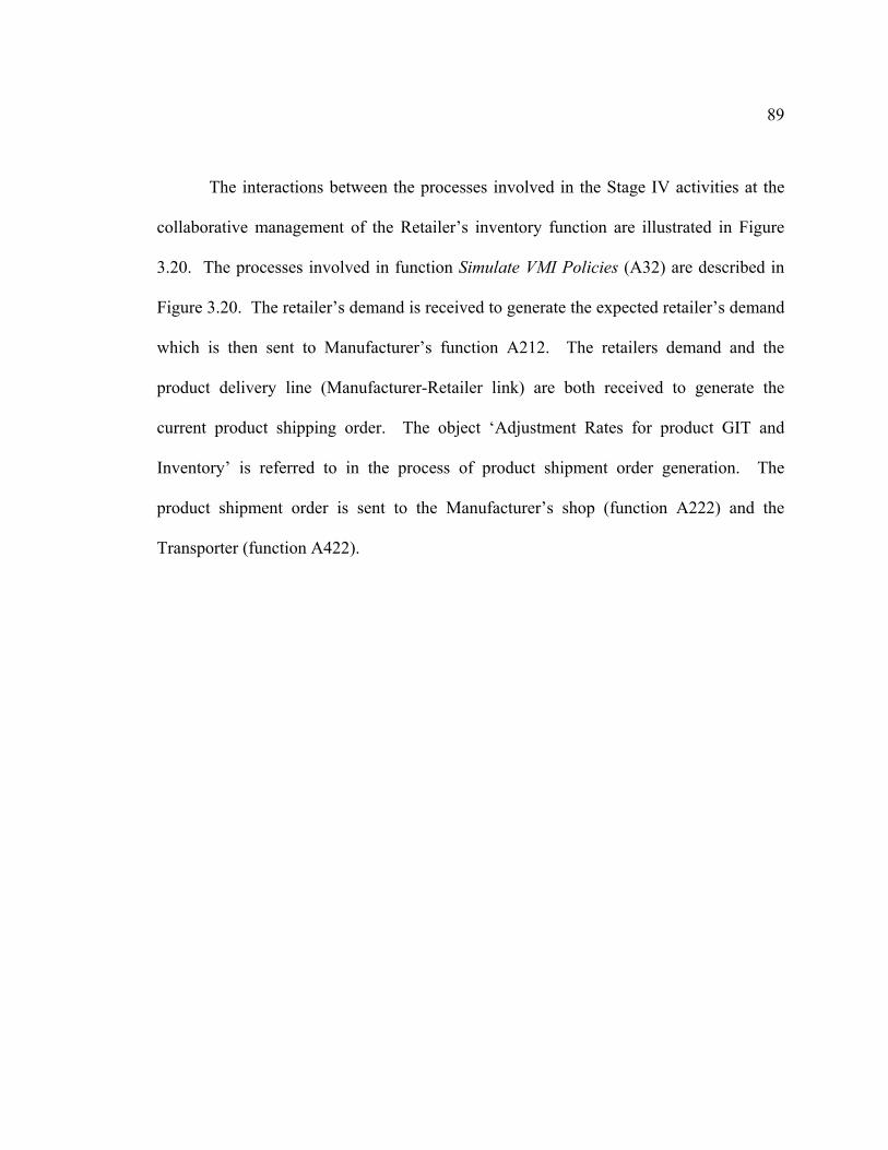
89


collaborative management of the Retailer’s inventory function are illustrated in Figure

3.20. The processes involved in function Simulate VMI Policies (A32) are described in

Figure 3.20. The retailer’s demand is received to generate the expected retailer’s demand

which is then sent to Manufacturer’s function A212. The retailers demand and the

product delivery line (Manufacturer-Retailer link) are both received to generate the

current product shipping order. The object ‘Adjustment Rates for product GIT and

Inventory’ is referred to in the process of product shipment order generation. The

product shipment order is sent to the Manufacturer’s shop (function A222) and the

Transporter (function A422).

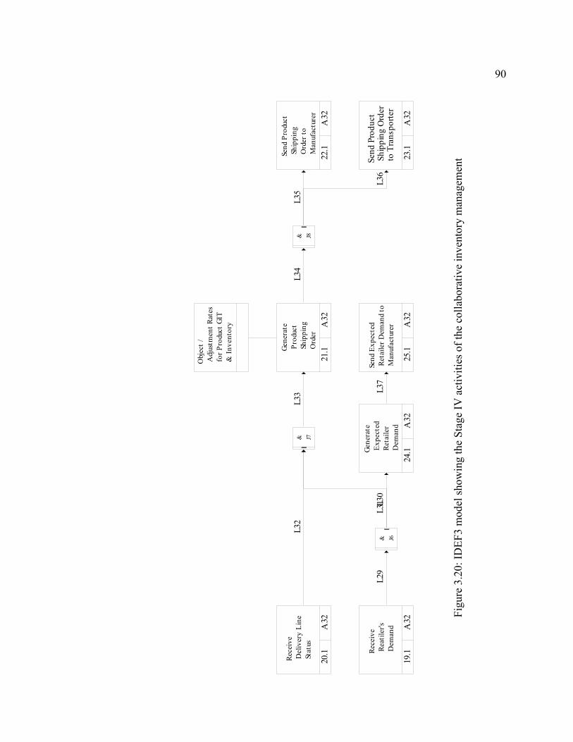
90

Send

Pro

duct

Shi

ppin

g O

rder

to T

rans

porte

r

23.1

A32

Send

Pro

duct

Shi

ppin

g O

rder

to M

anuf

actu

rer

22.1

A32

& J8

Gene

rate

Pro

duct

Shi

ppin

g O

rder

21.1

A32

Send

Exp

ecte

d R

etai

ler D

eman

d to

Man

ufac

ture

r

25.1

A32

Gene

rate

Exp

ecte

d R

etai

ler

Dem

and

24.1

A32

& J7

& J6

Rece

ive

Rea

tiler

's D

eman

d

19.1

A32

Rece

ive

Del

iver

y Li

ne S

tatu

s

20.1

A32

L32

L36

L35

L34

L33 L3

7L3

0L3

1L2

9

Obj

ect /

Adj

ustm

ent R

ates

for P

rodu

ct G

IT &

Inve

ntor

y

Figu

re 3

.20:

IDEF

3 m

odel

show

ing

the

Stag

e IV

act

iviti

es o

f the

col

labo

rativ

e in

vent

ory

man

agem

ent

91

3.5 Supply Chain Scenario: Policies and Assumptions

An overview of the three-echelon supply chain had been described in Section 3.1.

It is noted that the proposed architecture and methodology (refer Section 3.2) and the

underlying equations (Chapter 4) are applicable to a general supply chain with S

Suppliers, R Retailers, with N products flowing through the chain. Now, for the purpose

of experimentation the following structure of the supply chain is assumed:

• Supply chain consists of a Manufacturer, two Suppliers and three Retailers.

• Two products (Product 1 and Product 2) are produced by the Manufacturer.

• Demand exists for both products at all three Retailers.

• The bill-of-materials of both the products is composed of two components

(Component A and Component B).

• Component A is obtained from Supplier A and Component B is obtained from

Supplier B (the Suppliers manufacture the components).

• Infinite supply of raw materials for component production is assumed to be available

with the Suppliers.

• Transportation network transfer the components from the Suppliers to the

Manufacturer, and the products from the Manufacturer to the Retailers.

The assumptions and policies, adhered to in building the supply chain models for

use in various stages of the proposed methodology (refer Sections 3.2-3.4), are presented

in the following sub-sections.

92

3.5.1 Inventory Management Policies

The subsequent policies describe the inventory management procedures of the

supply chain players.

• The capacity for storage available at the Retailers, Manufacturer and the Suppliers are

assumed to be infinite.

• At the Retailers, the sales orders not fulfilled immediately are assumed to be lost,

which is a reasonable assumption at the retailer-level echelon where the sales is

delivery sensitive.

• At the Manufacturer and Suppliers, a backlog is maintained for unfulfilled orders.

• As part of the collaborative inventory management configuration, the Manufacturer

uses a min-max inventory policy to determine the quantity of the goods to be

dispatched to the Retailers. When the current level of inventory at Retailer falls

below the min level, the Manufacturer dispatches enough products to increase the

Retailer’s inventory to the max level (This constitutes the Vendor Managed Inventory

strategy).

• At the Supplier, the sales orders are received from the Manufacturer. If there is

sufficient inventory to cover the order then the required goods are immediately

dispatched. If there is not sufficient inventory, to cover the order, the quantity

available is dispatched and the rest of the order is backlogged.

93

3.5.2 Supply Chain Delay Assumptions

The various operations within the supply chain can be represented as finite delays

times. The assumptions that describe the delays that are part of the supply chain are

presented here.

• The accounting and purchasing delays, that is, the difference in the time of sales and

the time that sale is reflected in the current inventory levels is zero for all players.

• The mail delay, that is, the difference in the time an order is issued by the buyer and

the time the same order is received by the seller is zero between all the players.

• The information transmission delay, that is, the time taken to transmit any

information (other than orders) from one player to another is zero for all players.

• The production and transportation delays are represented as aggregated random

variables or modeled in detail depending upon the fidelity of the model.

3.5.3 Manufacturer’s Shop Floor

In the detailed DES models, the shop floor operations of the Manufacturer are

represented individually. The details of the shop layout and product flow information are

presented as follows (Figure 3.21):

• The Manufacturer’s shop is operated for three shifts per day of eight hour duration

each.

• Component A and Component B are the raw materials that are processed to produce

the final products, Product 1 and 2. One unit of final products, comprise of one unit

each of Components A and B.

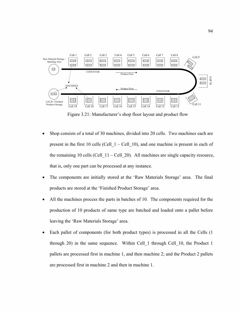
94

Cell 1 Cell 2 Cell 3 Cell 4 Cell 5 Cell 6 Cell 7 Cell 8

Cell 19 Cell 18 Cell 17 Cell 16 Cell 15 Cell 14 Cell 13 Cell 12

Cell 9

Cell 10

Cell 11

Raw Material Storage / Batching Area

Cell 20 / Finished Products Storage

CONVEYOR

CONVEYOR

MACHINES

Product Flow

Product Flow

Figure 3.21: Manufacturer’s shop floor layout and product flow

• Shop consists of a total of 30 machines, divided into 20 cells. Two machines each are

present in the first 10 cells (Cell_1 – Cell_10), and one machine is present in each of

the remaining 10 cells (Cell_11 – Cell_20). All machines are single capacity resource,

that is, only one part can be processed at any instance.

• The components are initially stored at the ‘Raw Materials Storage’ area. The final

products are stored at the ‘Finished Product Storage’ area.

• All the machines process the parts in batches of 10. The components required for the

production of 10 products of same type are batched and loaded onto a pallet before

leaving the ‘Raw Materials Storage’ area.

• Each pallet of components (for both product types) is processed in all the Cells (1

through 20) in the same sequence. Within Cell_1 through Cell_10, the Product 1

pallets are processed first in machine 1, and then machine 2; and the Product 2 pallets

are processed first in machine 2 and then in machine 1.

95

• The movement of the pallet of parts from the ‘Raw Materials Storage’ to Cell_1

through Cell_20 to the ‘Finished Product Storage’ is enabled using an accumulating

type conveyor. The conveyor travels at a speed of 5 ft per minute. The distances

between each cell are assumed to be 300 ft.

• The pallets are unloaded from the conveyor for operations in the cell, and then loaded

on to the conveyor once the operations are completed. An unloaded time of 15

minutes is assumed at each cell.

• The processing times, in hours, for each machine are defined as Triangular

distribution (14 machines), Normal distribution (13 machines) or Uniform

Distribution (3 machines). The means of the triangular and normal distributions have

been generated from UNIF[1.12, 1.76] using MinitabTM. The detailed information on

the selection of the processing times is presented in Appendix A, along with the table

of the processing time for all machines (see Table A.1).

• Infinite buffer capacity is assumed within each cell.

3.5.4 Suppliers’ Shop Floor

The Suppliers’ shop is constructed similar to the Manufacturer’s shop (see

Section 3.5.3)

• The Suppliers’ shop is operated for three shifts per day of eight hour duration each.

• Infinite supply of raw materials for production is assumed available with the

Suppliers.

• Supplier 1:

96

o Component A is the finished product,

o Supplier 1’s shop consists of a total of 20 machines, divided into 10 cells. Two

machines of unit capacity each are present in every cell.

o All machines process parts in batches of 10, with the product flowing from the

raw material storage, to cells 1 through 10, to the finished component storage.

o The inter-cell part routings are performed using a conveyor system similar to the

Manufacturer’s Shop.

o The processing times, in hours per batch, for each machine are defined as

Triangular distribution (10 machines), or Normal distribution (10 machines). The

means of the triangular and normal distributions have been generated from

UNIF[1.12, 1.76] using MinitabTM. The list of the processing time for all

machines is shown in Appendix A (see Table A.2).

• Supplier 2:

o Component B is the finished product,

o Supplier 2’s shop consists of a total of 30 machines, divided into 20 cells.

o The shop floor layout and part flow in Suppliers 2’s show is assumed to be

exactly the same as the Manufacturer, and hence not elaborated.

o The processing times, in hours, for each machine are defined as Triangular

distribution (10 machines), or Normal distribution (10 machines). The means of

the triangular and normal distributions have been generated from UNIF[1.12,

1.76] using MinitabTM. The list of the processing time for all machines is shown

in Appendix A (see Table A.3).

97

3.5.5 Transportation Network

In the detailed model of the transportation network, the individual transportation

activities are modeled in a distinct manner. The transportation network is characterized

as follows:

• A single transportation network is responsible for moving the components from the

Suppliers to the Manufacturer, and the products from the Manufacturer to the

Retailers.

• The mode of transport available is trucks. The maximum capacity of each truck is 10

units of components or 10 units of products.

• A truck makes a trip to the destination to deliver any quantity between 1 and 10.

• The velocity of trucks is modeled as Triangular (50, 55, 60). The units of parameters

are kilometers per hour.

• The distance between the Suppliers and the Manufacturer is 2500 km. The distance

between the Manufacturer and Retailers is 2500 km.

• Transporter operates a fleet of 25 trucks.

98

CHAPTER 4

MODELING THE SUPPLY CHAIN USING AGGREGATED MODELS

In this chapter, the aggregate-level system dynamic models used in the planning

stage (Stages I and II, see Figure 3.2) of the different members of the supply chain are

described. The background on the underlying logic behind the models, along with the

specific contributions of this research towards model development, is presented. The

generic models developed capture the mixing and variability in the production process,

capacitated resource allocation, and provides for spatial and lateral dimension of the

supply chain. Next, the models of individual members of the supply chain are defined

conceptually using modified causal loop diagrams (CLD), and then translated into

differential equation models.

4.1 Nomenclature Used

Index

t Index of time period {1…T} i Index of product {1…N} j Index of component{1…M} s Index of Supplier {1...S} r Index of Retailer {1…R}

Terms Description Measure

Manufacturer Production Ordering Terms Miα Fractional adjustment rate of WIP 1/time Miβ Fractional adjustment rate of inventory 1/time Miρ Exponential smoothing constant MiSALES SALES rate units/week

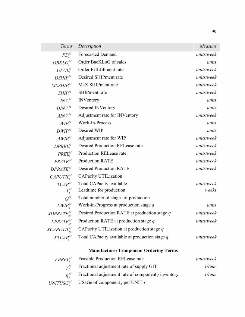
99

Terms Description Measure MiFD Forecasted Demand units/week MiOBKLG Order BacKLoG of sales units MiOFUL Order FULfillment rate units/week M

iDSHIP Desired SHIPment rate units/week M

iMXSHIP MaX SHIPment rate units/week M

iSHIP SHIPment rate units/week M

iINV INVentory units M

iDINV Desired INVentory units M

iAINV Adjustment rate for INVentory units/week M

iWIP Work-In-Process units M

iDWIP Desired WIP units M

iAWIP Adjustment rate for WIP units/week MiDPREL Desired Production RELease rate units/week MiPREL Production RELease rate units/week MiPRATE Production RATE units/week MiDPRATE Desired Production RATE units/week MiCAPUTIL CAPacity UTILization MTCAP Total CAPacity available units/week MiL Leadtime for production weeks MQ Total number of stages of production M

iqXWIP Work-in-Progress at production stage q units MiqXDPRATE Desired Production RATE at production stage q units/week MiqXPRATE Production RATE at production stage q units/week MiqXCAPUTIL CAPacity UTILization at production stage q M

qXTCAP Total CAPacity available at production stage q units/week

Manufacturer Component Ordering Terms

MiFPREL Feasible Production RELease rate units/week Mjγ Fractional adjustment rate of supply GIT 1/time Mjη Fractional adjustment rate of component j inventory 1/time MijUNITUSG USaGe of component j per UNIT i

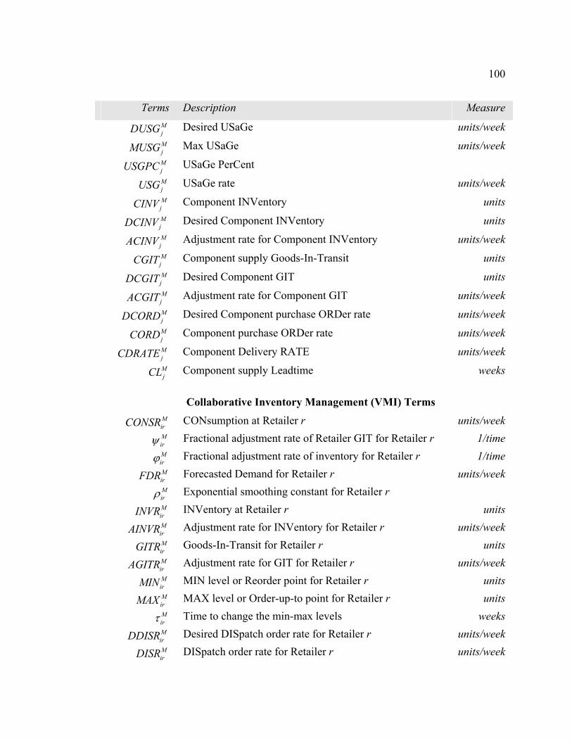
100

Terms Description Measure MjDUSG Desired USaGe units/week MjMUSG Max USaGe units/week MjUSGPC USaGe PerCent MjUSG USaGe rate units/week MjCINV Component INVentory units MjDCINV Desired Component INVentory units MjACINV Adjustment rate for Component INVentory units/week MjCGIT Component supply Goods-In-Transit units MjDCGIT Desired Component GIT units MjACGIT Adjustment rate for Component GIT units/week MjDCORD Desired Component purchase ORDer rate units/week MjCORD Component purchase ORDer rate units/week MjCDRATE Component Delivery RATE units/week MjCL Component supply Leadtime weeks

Collaborative Inventory Management (VMI) Terms

MirCONSR CONsumption at Retailer r units/week Mirψ Fractional adjustment rate of Retailer GIT for Retailer r 1/time Mirϕ Fractional adjustment rate of inventory for Retailer r 1/time MirFDR Forecasted Demand for Retailer r units/week Mirρ Exponential smoothing constant for Retailer r MirINVR INVentory at Retailer r units MirAINVR Adjustment rate for INVentory for Retailer r units/week MirGITR Goods-In-Transit for Retailer r units MirAGITR Adjustment rate for GIT for Retailer r units/week MirMIN MIN level or Reorder point for Retailer r units MirMAX MAX level or Order-up-to point for Retailer r units Mirτ Time to change the min-max levels weeks MirDDISR Desired DISpatch order rate for Retailer r units/week MirDISR DISpatch order rate for Retailer r units/week

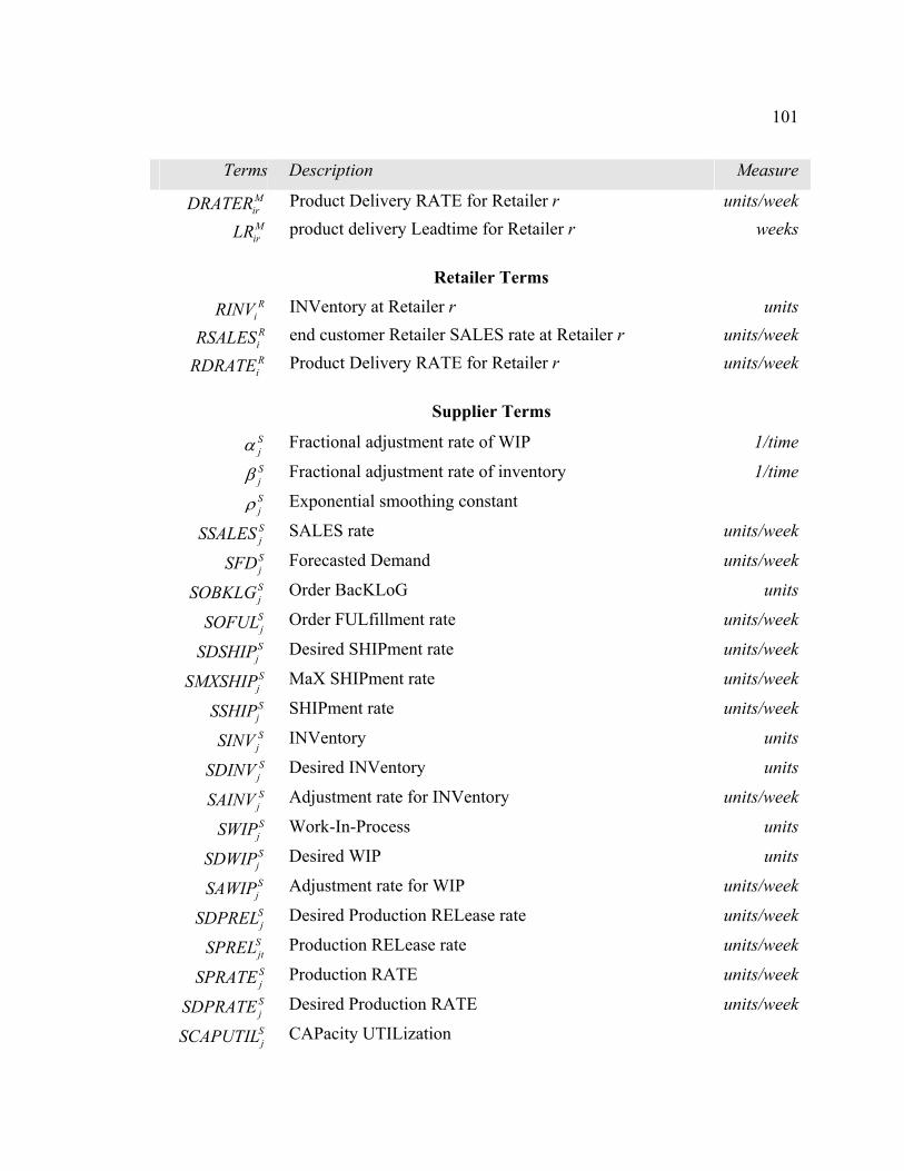
101

Terms Description Measure MirDRATER Product Delivery RATE for Retailer r units/week MirLR product delivery Leadtime for Retailer r weeks

Retailer Terms

RiRINV INVentory at Retailer r units RiRSALES end customer Retailer SALES rate at Retailer r units/week RiRDRATE Product Delivery RATE for Retailer r units/week

Supplier Terms

Sjα Fractional adjustment rate of WIP 1/time Sjβ Fractional adjustment rate of inventory 1/time Sjρ Exponential smoothing constant SjSSALES SALES rate units/week SjSFD Forecasted Demand units/week SjSOBKLG Order BacKLoG units SjSOFUL Order FULfillment rate units/week

SjSDSHIP Desired SHIPment rate units/week SjSMXSHIP MaX SHIPment rate units/week SjSSHIP SHIPment rate units/week SjSINV INVentory units SjSDINV Desired INVentory units SjSAINV Adjustment rate for INVentory units/week SjSWIP Work-In-Process units SjSDWIP Desired WIP units SjSAWIP Adjustment rate for WIP units/week SjSDPREL Desired Production RELease rate units/week

SjtSPREL Production RELease rate units/week SjSPRATE Production RATE units/week SjSDPRATE Desired Production RATE units/week SjSCAPUTIL CAPacity UTILization

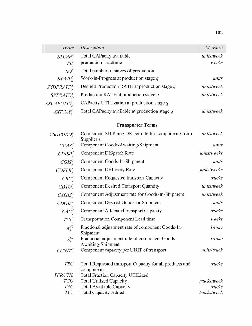
102

Terms Description Measure SSTCAP Total CAPacity available units/week SjSL production Leadtime weeks

SSQ Total number of stages of production SjqSXWIP Work-in-Progress at production stage q units SjqSXDPRATE Desired Production RATE at production stage q units/week SjqSXPRATE Production RATE at production stage q units/week

SjqSXCAPUTIL CAPacity UTILization at production stage q S

qSXTCAP Total CAPacity available at production stage q units/week

Transporter Terms

SjCSHPORD Component SHiPping ORDer rate for component j from

Supplier s units/week

SjCGAS Component Goods-Awaiting-Shipment units

SjCDISR Component DISpatch Rate units/weeks

SjCGIS Component Goods-In-Shipment units

SjCDELR Component DELivery Rate units/weeks

SjCRC Component Requested transport Capacity trucks

SjCDTQ Component Desired Transport Quantity units/week

SjCAGIS Component Adjustment rate for Goods-In-Shipment units/week

SjCDGIS Component Desired Goods-In-Shipment units

SjCAC Component Allocated transport Capacity trucks SjTCL Transportation Component Lead time weeks

CSjπ Fractional adjustment rate of component Goods-In-

Shipment 1/time

CSjλ Fractional adjustment rate of component Goods-

Awaiting-Shipment 1/time

SjCUNIT Component capacity per UNIT of transport units/truck

TRC Total Requested transport Capacity for all products and

components trucks

TFRUTIL Total Fraction Capacity UTILized TCU Total Utilized Capacity trucks/week TAC Total Available Capacity trucks TCA Total Capacity Added trucks/week

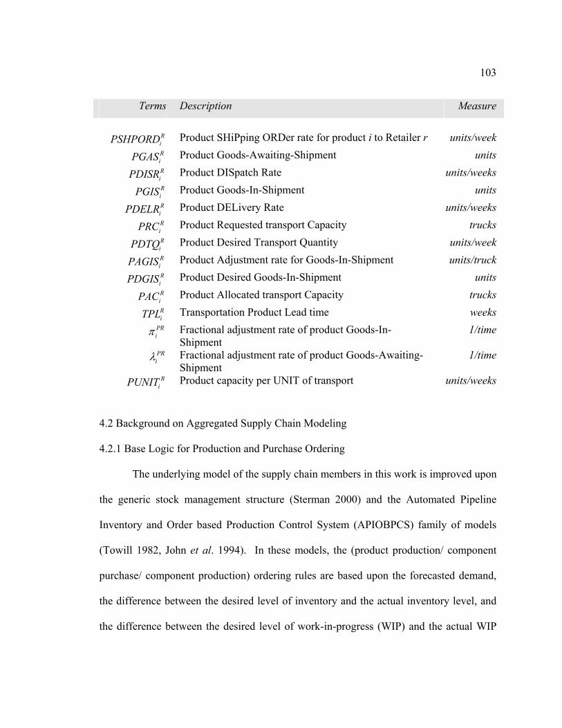
103

Terms Description Measure

RiPSHPORD Product SHiPping ORDer rate for product i to Retailer r units/week

RiPGAS Product Goods-Awaiting-Shipment units

RiPDISR Product DISpatch Rate units/weeks

RiPGIS Product Goods-In-Shipment units

RiPDELR Product DELivery Rate units/weeks

RiPRC Product Requested transport Capacity trucks

RiPDTQ Product Desired Transport Quantity units/week

RiPAGIS Product Adjustment rate for Goods-In-Shipment units/truck

RiPDGIS Product Desired Goods-In-Shipment units

RiPAC Product Allocated transport Capacity trucks RiTPL Transportation Product Lead time weeks

PRiπ Fractional adjustment rate of product Goods-In-

Shipment 1/time

PRiλ Fractional adjustment rate of product Goods-Awaiting-

Shipment 1/time

RiPUNIT Product capacity per UNIT of transport units/weeks

4.2 Background on Aggregated Supply Chain Modeling

4.2.1 Base Logic for Production and Purchase Ordering

The underlying model of the supply chain members in this work is improved upon

the generic stock management structure (Sterman 2000) and the Automated Pipeline

Inventory and Order based Production Control System (APIOBPCS) family of models

(Towill 1982, John et al. 1994). In these models, the (product production/ component

purchase/ component production) ordering rules are based upon the forecasted demand,

the difference between the desired level of inventory and the actual inventory level, and

the difference between the desired level of work-in-progress (WIP) and the actual WIP

104

level. The ordering rule is a very general replenishment rule, the advantages of which

include (Disney et al. 2003):

• ability to represent material requirements planning (MRP) systems as a special case

(Disney 2001),

• ability to represent order-up-to systems and many variants as special cases

(Dejonckheere 2003),

• lean and agile scheduling policies can be incorporated (Dejonckheere 2003),

• reentrant manufacturing systems can be modeled (Tang and Naim 2004),

• Vendor Managed Inventory (VMI) strategy can be coupled (Disney 2001, Disney et

al. 2003),

• representative of industrial performance in UK (Coyle 1977), and

• represents human behavior models whilst playing the Beer Game (John et al. 1994).

In this research, the above ordering rule is adapted to represent the production release and

the component purchase ordering rules at the Manufacturer, and the production release

rule at the Suppliers. Also, a variant of the stock management structure is applied to the

product dispatch ordering rule for the Retailers and the transportation dispatching rule at

the Transporter.

4.2.1.1 Improvements over Existing Models

The system dynamic models developed in this research are a significant

contribution, which improves over the APIOBPCS model and other SD supply chain

models in the following aspects:

105

• Representation of the production process at the Manufacturer and Suppliers using a

higher order material delay rather than a fixed pipeline delay. This allows for a more

accurate account of the production process by capturing the mixing of products and

variability in the processing times.

• Explicit representation of the frequency of information update, through the use of a

sampling interval, to study its effect on the system stability.

• Production capacity constraints are included in the Manufacturer and Suppliers model,

and the transportation capacity constraints are included in the Transporter model.

Both the capacity constraints affect the dynamic responses of the supply chain.

• Maintenance of order backlog at the Manufacturer, Suppliers and the Transporter to

ensure that the orders not fulfilled immediately are not lost, and also to account for

the possible administrative activities in order processing.

• Representation of raw material component inventory at the Manufacturer which

affects the production release ordering.

• Production of products at the Manufacturer composed of multiple components

obtained from different Suppliers. Such lateral dimension creates a consolidation of

goods at the Manufacturer, which reflect the operations of typical supply chains.

• Transportation network (Transporter) is explicitly modeled rather than a fixed

pipeline delay, which allows for capturing the transportation resource allocation.

This affects the lead-times and hence the dynamics of the supply chain.

• Retailer’s dispatching rule is based on a MIN-MAX inventory policy to mimic the

realistic operations at the retailer-level echelons of the supply chain.

106

• Spatial dimension of the supply chain has been created by modeling multiple

Suppliers (two) and multiple Retailers (three). This results in consolidations in

resource capacity allocation at the Manufacturer and Transporter.

The conceptual model and the underlying equations of the Automated Pipeline

Inventory and Order based Production Control System (APIOBPCS) model (John et al.

1994) is shown in Appendix B.

4.2.2 Causal Loop Diagrams

In the following subsections, the system dynamic models of individual members

of the supply chain are defined conceptually and then translated into differential equation

models which can be readily simulated. Causal Loop Diagrams (CLDs) are used to

represent the conceptual feedback structure of systems (Richardson 1986, Sterman 2000).

The CLDs are interpreted as follows:

• The CLD consists of variables that are connected by causal links, represented by

arrows, indicating the influence amongst the variables.

• In each causal link, the variable at the tail of the arrow is called as the independent

variable and the variable at the head of the arrow is called as the dependent variable.

• A positive (+) causal link means that when the independent variable increases

(decreases), the dependent variable increases above (decreases below) what would

have been if the independent variable did not change.

107

• A negative (–) causal link means that when the independent variable increases

(decreases), the dependent variable decreases below (increases above) what would

have been if the independent variable did not change.

The main difficulty of the CLDs is that they do not capture the stock and flow structure

of the system (Richardson 1986, Richardson 1997, Sterman 2000, Binder et al. 2004),

which is required to model the dynamic system exactly and derive the appropriate

differential equations. Such a model can however be modeled as Stock and Flow

Diagrams (SFDs) (Sterman 2000). Stocks, represented by rectangles, are accumulations

that characterize the state of the system, provide inertia and memory, acts as a source of

delay and create disequilibrium dynamics (Sterman 2000). It is noted that the stocks only

change through the flows (or flow rates) and there is no causal link directly into the

stocks. This raises the question of how to develop the SFDs from CLDs (Binder et al.

2004). Though there are several methods proposed in recent works to develop SFD from

CLD (Binder et. al 2004 and Burns 2001), it requires the modeler to have in-depth

knowledge of the system considered. In this work, the CLDs are used as a system

descriptive and communication tool. Hence, the stocks and flows shall be explicitly

included as part of the causal diagram to enhance clarity (Sterman 2000).

4.3 System Dynamics Model of Manufacturer

The Manufacturer performs product production ordering and inventory control

(demand forecasting, customer order fulfillment, determining the production release

quantities, and production process), raw material component ordering, and the

108

collaborative management of Retailer’s inventory. The product production ordering and

inventory control functions have been identified based on their direct influence on the

production-inventory control system and based on the past research. The raw material

component ordering and the collaborative management of Retailer’s inventory have been

identified based on the supply chain-wide interactions between Supplier-Manufacturer

and Manufacturer-Retailer, respectively. The conceptual models are shown in Figures

4.1 through 4.4 using CLD with the stock-flow structure, where Figure 4.1 depicts the

product production and inventory management, Figure 4.2 depicts the product production

process, Figure 4.3 depicts the component purchase ordering and Figure 4.4 depicts the

collaborative management of the Retailer’s inventory. The underlying equations

governing each function, along with their validity and appropriateness, are as described in

the following sections.

4.3.1 Product Production Ordering and Inventory Control

4.3.1.1 Demand Forecasting

The Manufacturer is assumed to forecast demand ( MiFD ) of its products based on

a first order exponential smoothing of the customer sales rate ( MiSALES ), with a

smoothing constant Miρ (Figure 4.1, top left):

1 1[ ] / ( )M M Mi it itd FD dt SALES FD M

iρ− −= − ⋅ (4.3.1)

For the purpose of this research, it is desirable to minimize the impact of forecasting

methods on the system response. Based on pilot experiments by Venkateswaran and Son

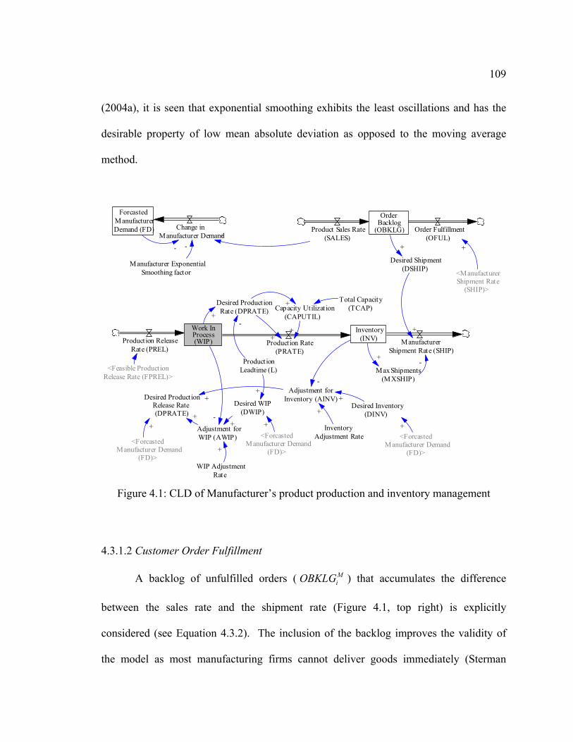
109

(2004a), it is seen that exponential smoothing exhibits the least oscillations and has the

desirable property of low mean absolute deviation as opposed to the moving average

method.

Work InProcess(WIP)

Inventory(INV)Production Rate

(PRATE)Production Release

Rate (PREL)Manufacturer

Shipment Rate (SHIP)

Max Shipments(MXSHIP)

-+

Adjustment forInventory (AINV)

Adjustment forWIP (AWIP)

Desired ProductionRelease Rate(DPRATE)

Desired Inventory(DINV)

Desired WIP(DWIP)

-+

-

+

+

+

WIP AdjustmentRate

+

InventoryAdjustment Rate

+

ProductionLeadtime (L)

+

<Feasible ProductionRelease Rate (FPREL)>

Desired Product ionRate (DPRATE)+

-

+

Total Capacity(TCAP)Capacity Utilizat ion

(CAPUTIL)

+

+

ForcastedManufacturerDemand (FD) Change in

Manufacturer Demand

Manufacturer ExponentialSmoothing factor

--

<ForcastedManufacturer Demand

(FD)>


(FD)><Forcasted

Manufacturer Demand(FD)>

+ + +

OrderBacklog

(OBKLG)Product Sales Rate(SALES)

Order Fulfillment(OFUL)

<ManufacturerShipment Rate

(SHIP)>

+

Desired Shipment(DSHIP)

++

+

Figure 4.1: CLD of Manufacturer’s product production and inventory management

4.3.1.2 Customer Order Fulfillment

A backlog of unfulfilled orders ( MiOBKLG ) that accumulates the difference

between the sales rate and the shipment rate (Figure 4.1, top right) is explicitly

considered (see Equation 4.3.2). The inclusion of the backlog improves the validity of

the model as most manufacturing firms cannot deliver goods immediately (Sterman

110

2000). The shipment rate ( MiSHIP ) of the physical goods is determined as a function of

the current order backlog and the inventory in stock, to ensure that the shipment rate does

not exceed the inventory in hand (see Equations 4.3.3 – 4.3.5). The shipment rate, in turn

determines the order fulfillment rate ( MiOFUL ). The shipment rate refers to the physical

flow and the order fulfillment rate refers to the information flow.

[ ] /M Mi itd OBKLG dt SALES OFUL= − M

it

]

(4.3.2)

[ ,M Mit it itSHIP f DSHIP MXSHIP= M (4.3.3)

M Mit itDSHIP OBKLG= (4.3.4)

M Mit itMXSHIP INV= (4.3.5)

M Mit itOFUL SHIP= (4.3.6)

4.3.1.3 Production Ordering

The production ordering aspect of the Manufacturer determines the desired

production release quantities ( MiDPREL ) using the ordering rule (Equation 4.3.7), based

upon the forecasted demand, the difference between the desired level of WIP ( MiDWIP )

and the current WIP level ( MiWIP ), and difference between the desired level of inventory

( MiDINV ) and the current inventory level ( M

iINV ) (Figure 4.1):

1M M Mit it it itDPREL FD AWIP AINV−= + + M

)

(4.3.7)

1(M M M Mit i it itAWIP DWIP WIPα −= ⋅ − (4.3.8)

1(M M M Mit i it itAINV DINV INVβ )−= ⋅ − (4.3.9)

111

The fractional adjustment rate for WIP ( Miα ) describes how much of the discrepancy

between the desired and current levels of WIP are to be added to the production release

order. The fractional adjustment rate for inventory ( Miβ ) describes how much of the

discrepancy between the desired and current levels of inventory are to be added to the

production release order.

Based on the Little’s Law, the desired WIP ( MiDWIP ) in the system is set to yield

the desired throughput, given the lead time ( MiL ) (see Equation 4.3.10). The desired

throughput is set equal to the forecasted demand. To provide adequate coverage of

inventory, the manufacturer seeks to maintain a desired level of inventory ( MiDINV ) set

equal to the forecasted demand (see Equation 4.3.11). Also, the inventory level ( MiINV )

accumulates the difference in the production rate ( MiPRATE ) and the shipment rate (see

Equation 4.3.12). The WIP level ( MiWIP ) and the production rate are modeled as higher

order delays, as explained in detailed in the Section 4.3.1.4.

1M M M

it it itDWIP FD L−= ⋅ (4.3.10)

1M M

it itDINV FD −= (4.3.11)

[ ] /M Mi itd INV dt PRATE SHIP= − M

it (4.3.12)

4.3.1.4 Production Process

The production process (Figure 4.1) is typically modeled as a fixed pipeline delay

(Towill 1982, John et al. 1994, Towill et al. 2001). However, this does not capture the

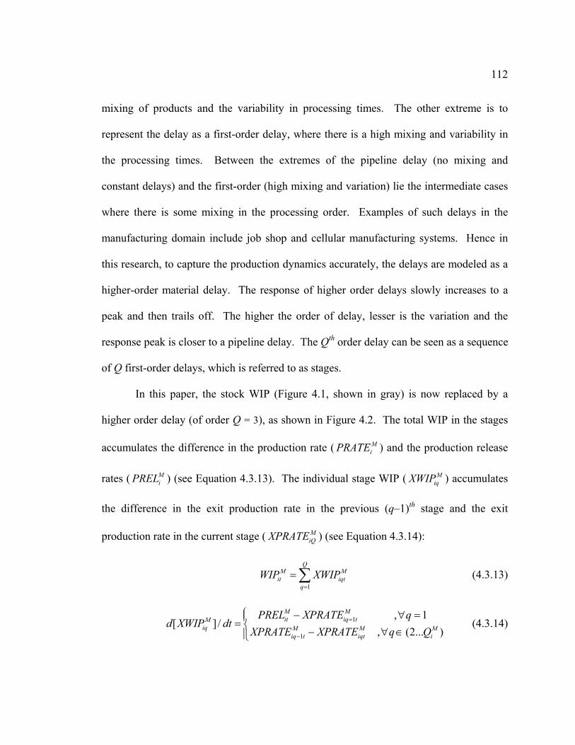
112

mixing of products and the variability in processing times. The other extreme is to

represent the delay as a first-order delay, where there is a high mixing and variability in

the processing times. Between the extremes of the pipeline delay (no mixing and

constant delays) and the first-order (high mixing and variation) lie the intermediate cases

where there is some mixing in the processing order. Examples of such delays in the

manufacturing domain include job shop and cellular manufacturing systems. Hence in

this research, to capture the production dynamics accurately, the delays are modeled as a

higher-order material delay. The response of higher order delays slowly increases to a

peak and then trails off. The higher the order of delay, lesser is the variation and the

response peak is closer to a pipeline delay. The Qth order delay can be seen as a sequence

of Q first-order delays, which is referred to as stages.

In this paper, the stock WIP (Figure 4.1, shown in gray) is now replaced by a

higher order delay (of order Q = 3), as shown in Figure 4.2. The total WIP in the stages

accumulates the difference in the production rate ( MiPRATE ) and the production release

rates ( MiPREL ) (see Equation 4.3.13). The individual stage WIP ( M

iqXWIP ) accumulates

the difference in the exit production rate in the previous (q–1)th stage and the exit

production rate in the current stage ( MiQXPRATE ) (see Equation 4.3.14):

1

QM M

it iqtq

WIP XWIP=

= ∑ (4.3.13)

1

1

, 1[ ] /

, (2... )

M Mit iq tM

iq M Miq t iqt i

PREL XPRATE qd XWIP dt MXPRATE XPRATE q Q

=

−

⎧ − ∀⎪= ⎨ − ∀ ∈⎪⎩

= (4.3.14)

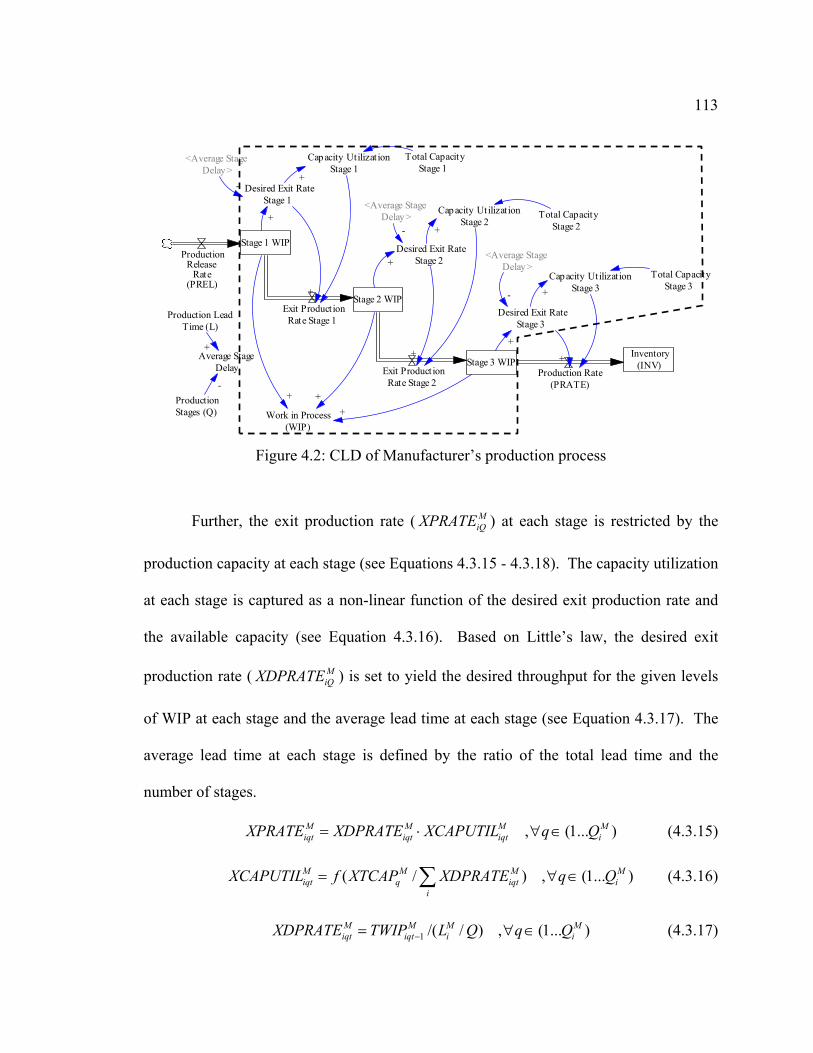
113

Stage 1 WIP

Stage 2 WIP

Stage 3 WIPInventory

(INV)

ProductionRelease

Rate(PREL)

Production Rate(PRATE)

Exit Product ionRate Stage 1

Exit Product ionRate Stage 2

Production LeadTime (L)

Work in Process(WIP)

+ ++

Desired Exit RateStage 1



Capacity Utilizat ionStage 1

Capacity UtilizationStage 2

Capacity Utilizat ionStage 3

Total CapacityStage 1



+

+

+

+

+

++

+

+

ProductionStages (Q)

Average StageDelay

+

-

<Average StageDelay>



-

-

-

Figure 4.2: CLD of Manufacturer’s production process

Further, the exit production rate ( MiQXPRATE ) at each stage is restricted by the

production capacity at each stage (see Equations 4.3.15 - 4.3.18). The capacity utilization

at each stage is captured as a non-linear function of the desired exit production rate and

the available capacity (see Equation 4.3.16). Based on Little’s law, the desired exit

production rate ( MiQXDPRATE ) is set to yield the desired throughput for the given levels

of WIP at each stage and the average lead time at each stage (see Equation 4.3.17). The

average lead time at each stage is defined by the ratio of the total lead time and the

number of stages.

, (1... )M M Miqt iqt iqt i

MXPRATE XDPRATE XCAPUTIL q Q= ⋅ ∀ ∈ (4.3.15)

( / ) , (1... )M M Miqt q iqt i

i

MXCAPUTIL f XTCAP XDPRATE q Q= ∀ ∈∑ (4.3.16)

1 /( / ) , (1... )M M Miqt iqt i i

MXDPRATE TWIP L Q q Q−= ∀ ∈ (4.3.17)

114

M Mit iQtPRATE XPRATE= (4.3.18)

4.3.2 Raw Material Component Ordering

In this research, the raw material component inventory is explicitly modeled to

capture the supply side dynamics of the Manufacturer (Figure 4.3). Now, the production

process can begin only if there is sufficient component inventory. The production release

rate is hence set equal to the feasible production release rate ( MiFPREL ), which is a

function of the component usage percent ( MjUSGPC ), and the desired product release:

M M Mit it jt itPREL FPREL USGPC DPREL= = ⋅ M (4.3.19)

The component usage percent (Equation 4.3.20), is defined as a non-linear function of the

desired component usage ( MjDUSG ) and the current levels of component inventory

( MjCINV ). The desired component usage (Equation 4.3.22) captures the total quantity of

component j desired, which can be simply given by the sum of the product of the desired

production release ( MiDPREL ) and M

ijUNITUSG for all products i.

(4.3.20) ( /M Mjt jt jtUSGPC f DUSG MXUSG= )M

M Mjt jtMXUSG CINV= (4.3.21)

M Mjt it ij

iDUSG DPREL UNITUSG= ⋅ M∑ (4.3.22)

M Mjt jt jtUSG DUSG USGPC= ⋅ M (4.3.23)

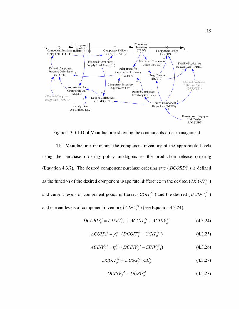
115

Componentgoods in

transit (CGIT)

ComponentInventory(CINV)Component Delivery

Rate (CDRATE)Component PurchaseOrder Rate (PORD)

Component UsageRate (USG)

Adjustment forComponent Inventory

(ACINV)

Adjustment forComponent GIT

(ACGIT)

Desired ComponentPurchase Order Rate

(DPORD)

Desired ComponentInventory (DCINV)

Desired ComponentGIT (DCGIT)

+

++

+

Component InventoryAdjustment Rate

+

Desired ComponentUsage Rate (DUSG)

Component Usage p erUnit Product(UNITUSG)

Maximum ComponentUsage (MUSG)

+

+

Feasible ProductionRelease Rate (FPREL)

-

+

+

+

Supp ly LineAdjustment Rate

+<Desired ComponentUsage Rate (DUSG)>

+

Expected ComponentSupp ly Lead Time (CL)

+

+

+

Usage Percent(USGPC)

+

+

+

+

<Desired ProductionRelease Rate(DPRATE)>

+

+

Figure 4.3: CLD of Manufacturer showing the components order management

The Manufacturer maintains the component inventory at the appropriate levels

using the purchase ordering policy analogous to the production release ordering

(Equation 4.3.7). The desired component purchase ordering rate ( MjDCORD ) is defined

as the function of the desired component usage rate, difference in the desired ( MjDCGIT )

and current levels of component goods-in-transit ( MjCGIT ) and the desired ( M

jDCINV )

and current levels of component inventory ( MjCINV ) (see Equation 4.3.24):

1M M Mjt jt jt jtDCORD DUSG ACGIT ACINV−= + + M

)

(4.3.24)

1(M M M Mjt j jt jtACGIT DCGIT CGITγ −= ⋅ − (4.3.25)

1(M M M Mjt j jt jtACINV DCINV CINVη )−= ⋅ − (4.3.26)

M Mjt jt jtDCGIT DUSG CL= ⋅ M (4.3.27)

M Mjt jtDCINV DUSG= (4.3.28)

116

[ ] /M Mj jtd CGIT dt CORD CDRATE= − M

jt (4.3.29)

[ ] /M Mj jtd CINV dt CDRATE USG= − M

jt (4.3.30)

M Mjt jtCORD DCORD= (4.3.31)

The fractional adjustment rates of component goods-in-transit ( Mjγ ) and

component inventory ( Mjη ) describes the rate at which the shortfall in the desired and

current levels of component GIT and component inventory are corrected, respectively.

It is recalled that the Manufacturer and the Supplier are independent members

with no goal congruence. Hence, from the perspective of the Manufacturer, the supply

side is modeled as a pipeline delay, where the component delivery rate ( MjCDRATE ) is

modeled as a pipeline delay of the component ordering rate ( MjCORD ) with a lead time

( MiCL ):

(4.3.32) (M Mjt j t CLCDRATE CORD −= )

4.4 System Dynamics Model for Collaborative Management of Retailer’s Inventory

The Manufacturer manages the Retailer’s inventory as part of their collaborative

configuration using vendor managed inventory strategy (Figure 4.4). The Manufacturer

obtains the current inventory levels ( MirINVR ) and end customer sales or consumption

data ( MirCONSR ) from the Retailers; and uses a MIN-MAX inventory control policy to

determine the dispatch quantities to the Retailer.

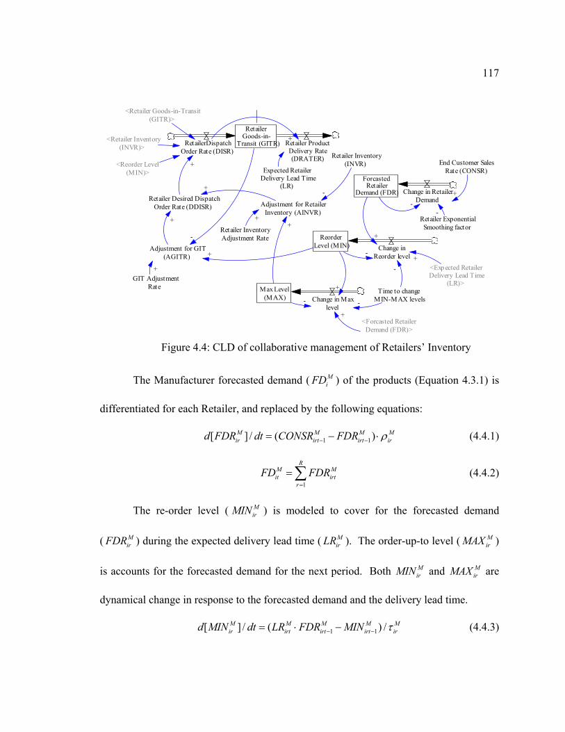
117

ReorderLevel (MIN) Change in

Reorder level

Time to changeMIN-MAX levels

-

-

ForcastedRetailer

Demand (FDR) Change in RetailerDemand

Retailer ExponentialSmoothing factor

--

+

Max Level(MAX) Change in Max

level-

+

-

Retailer Desired DispatchOrder Rate (DDISR)

Retailer Goods-in-

Transit (GITR) Retailer ProductDelivery Rate(DRATER)

Expected RetailerDelivery Lead Time

(LR)

RetailerDispatchOrder Rate (DISR)

<Expected RetailerDelivery Lead Time

(LR)>

+Adjustment for GIT

(AGITR)

Adjustment for RetailerInventory (AINVR)

+

+

-

+

+

GIT AdjustmentRate

Retailer InventoryAdjustment Rate

+

+

<Forcasted RetailerDemand (FDR)>

+

<Reorder Level(MIN)>

+

<Retailer Goods-in-Transit(GITR)>

+ End Customer SalesRate (CONSR)

+

Retailer Inventory(INVR)

-

<Retailer Inventory(INVR)>

Figure 4.4: CLD of collaborative management of Retailers’ Inventory

The Manufacturer forecasted demand ( MiFD ) of the products (Equation 4.3.1) is

differentiated for each Retailer, and replaced by the following equations:

1 1[ ] / ( )M M Mir irt irt ird FDR dt CONSR FDR Mρ− −= − ⋅ (4.4.1)

1

RM Mit irt

rFD FDR

=

= ∑ (4.4.2)

The re-order level ( MirMIN ) is modeled to cover for the forecasted demand

( MirFDR ) during the expected delivery lead time ( M

irLR ). The order-up-to level ( MirMAX )

is accounts for the forecasted demand for the next period. Both MirMIN and M

irMAX are

dynamical change in response to the forecasted demand and the delivery lead time.

1 1[ ] / ( ) /M M M Mir irt irt irt ird MIN dt LR FDR MIN Mτ− −= ⋅ − (4.4.3)

118

1 1 1[ ] / ( ) /M M M Mir irt irt irt ird MAX dt FDR MIN MAX Mτ− − −= + − (4.4.4)

A MIN-MAX inventory control policy is employed, in which the dispatch order is

generated when the inventory level fall below a set re-order level. The dispatch ordering

rule also accounts for the orders in the pipeline, that is, dispatch orders placed but not yet

delivered to the Retailers.

(4.4.5) , ( )

0 ,

M M MM irt irt irt irtirt

DDISR if GITR INVR MINDISR

otherwise⎧ + ≤

= ⎨⎩

M

M Mirt irt irtDDISR AGITR AINVR= + M

1)−

1)−

(4.4.6)

(4.4.7) 1(M M M Mirt ir irt irtAGITR MIN GITRψ −= ⋅ −

(4.4.8) 1(M M M Mirt ir irt irtAINVR MAX INVRϕ −= ⋅ −

[ ] /M Mir irt irtd GITR dt DISR DRATER= − M (4.4.9)

M Mit irt

RSALES DISR=∑ (4.4.10)

The fractional adjustment rates of product goods-in-transit ( Mirψ ) and product

inventory ( Mirϕ ) describes the rate at which the shortfall in the desired and current levels

of product GIT and product inventory are corrected, respectively. Also, the delivery side

is modeled as a pipeline delay, where the product delivery rate ( MirDRATER ) is modeled

as a pipeline delay of the product purchase ordering rate ( MirDISR ) with a lead time

( MirLR ):

(4.4.11) ,M Mirt ir t RLDRATER DISR −=

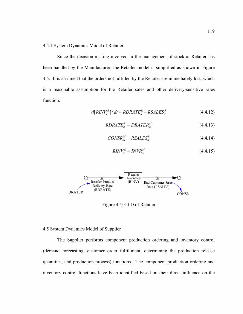
119

4.4.1 System Dynamics Model of Retailer

Since the decision-making involved in the management of stock at Retailer has

been handled by the Manufacturer, the Retailer model is simplified as shown in Figure

4.5. It is assumed that the orders not fulfilled by the Retailer are immediately lost, which

is a reasonable assumption for the Retailer sales and other delivery-sensitive sales

function.

(4.4.12) [ ] /R Ri itd RINV dt RDRATE RSALES= − R

it

M Rit irtRDRATE DRATER= (4.4.13)

M Rirt itCONSR RSALES= (4.4.14)

Rit irt

MRINV INVR= (4.4.15)

RetailerInventory(RINV) End Customer Sales

Rate (RSALES)Retailer ProductDelivery Rate(RDRATE)

DRATER CONSR

Figure 4.5: CLD of Retailer

4.5 System Dynamics Model of Supplier

The Supplier performs component production ordering and inventory control

(demand forecasting, customer order fulfillment, determining the production release

quantities, and production process) functions. The component production ordering and

inventory control functions have been identified based on their direct influence on the

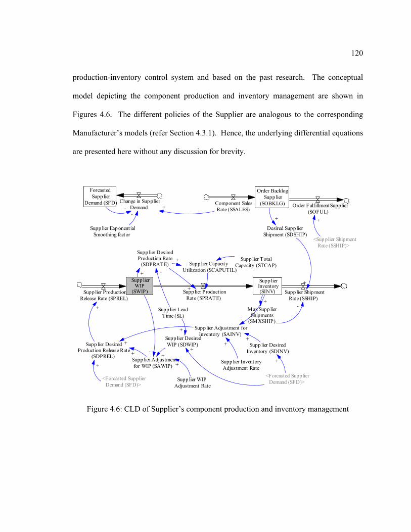
120

production-inventory control system and based on the past research. The conceptual

model depicting the component production and inventory management are shown in

Figures 4.6. The different policies of the Supplier are analogous to the corresponding

Manufacturer’s models (refer Section 4.3.1). Hence, the underlying differential equations

are presented here without any discussion for brevity.

Supp lierWIP

(SWIP)

Supp lierInventory(SINV)Supp lier Production

Rate (SPRATE)Supp lier Production

Release Rate (SPREL)Supp lier Shipment

Rate (SSHIP)

Max Supp lierShipments

(SMXSHIP)

-+

Supp lier Adjustment forInventory (SAINV)

Supp lier Adjustmentfor WIP (SAWIP)

Supp lier DesiredProduct ion Release Rate

(SDPREL)

Supp lier DesiredInventory (SDINV)

Supp lier DesiredWIP (SDWIP)

+

-

+

+

+

Supp lier WIPAdjustment Rate

+ Supp lier InventoryAdjustment Rate

+-

Supp lier LeadTime (SL)

+

Supp lier DesiredProduct ion Rate

(SDPRATE)Supp lier Total

Capacity (STCAP)Supp lier CapacityUtilization (SCAPUTIL)

+

+ -

+

+

ForcastedSupp lier

Demand (SFD) Change in SupplierDemand

Supp lier ExponentialSmoothing factor

--

Order BacklogSupp lier

(SOBKLG)Component SalesRate (SSALES)

Order FulfillmentSupplier(SOFUL)

Desired Supp lierShipment (SDSHIP)

+

<Supplier ShipmentRate (SSHIP)>

+

+

<Forcasted SupplierDemand (SFD)>

<Forcasted SupplierDemand (SFD)>

+

+

+

+

Figure 4.6: CLD of Supplier’s component production and inventory management

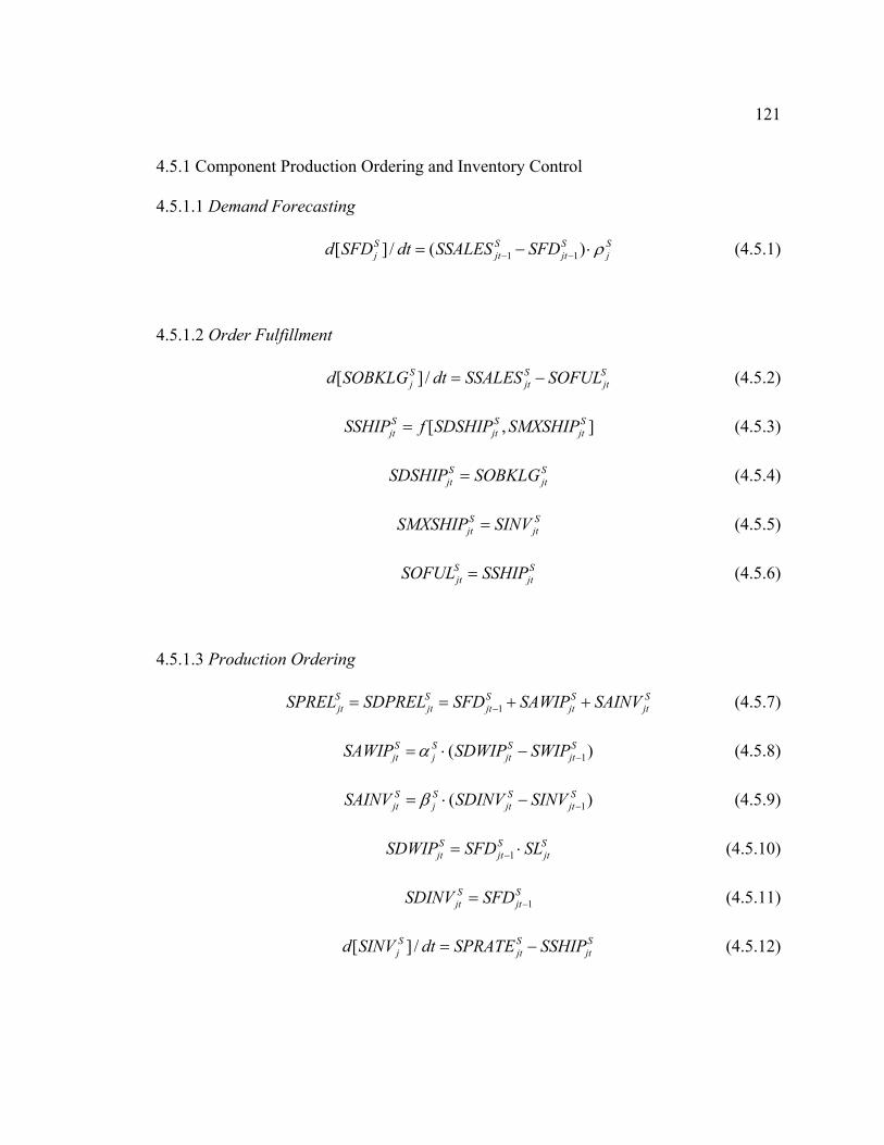
121

4.5.1 Component Production Ordering and Inventory Control

4.5.1.1 Demand Forecasting

1 1[ ] / ( )S Sj jtd SFD dt SSALES SFDS S

jt jρ− −= − ⋅

Sjt

]S

S

S

S

S

)

)

(4.5.1)

4.5.1.2 Order Fulfillment

(4.5.2) [ ] /S Sj jtd SOBKLG dt SSALES SOFUL= −

(4.5.3) [ ,S Sjt jt jtSSHIP f SDSHIP SMXSHIP=

(4.5.4) Sjt jtSDSHIP SOBKLG=

(4.5.5) Sjt jtSMXSHIP SINV=

(4.5.6) Sjt jtSOFUL SSHIP=

4.5.1.3 Production Ordering

(4.5.7) 1S S S Sjt jt jt jt jtSPREL SDPREL SFD SAWIP SAINV−= = + +

(4.5.8) 1(S S S Sjt j jt jtSAWIP SDWIP SWIPα −= ⋅ −

1(S S S Sjt j jt jtSAINV SDINV SINVβ −= ⋅ − (4.5.9)

(4.5.10) 1S Sjt jt jtSDWIP SFD SL−= ⋅ S

S 1Sjt jtSDINV SFD −= (4.5.11)

(4.5.12) [ ] /S Sj jtd SINV dt SPRATE SSHIP= − S

jt

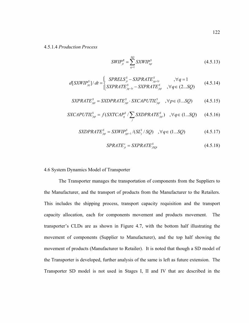
122

4.5.1.4 Production Process

(4.5.13) 1

SQRjt iqt

q

SWIP SXWIP=

= ∑ S

=

∈

(4.5.14) 1

1

, 1[ ] /

, (2... )

S Sjt jq tS

jq S Sjq t jqt

SPRELS SXPRATE qd SXWIP dt

SXPRATE SXPRATE q SQ=

−

⎧ − ∀⎪= ⎨ − ∀ ∈⎪⎩

(4.5.15) , (1... )S S Sjqt jqt jqtSXPRATE SXDPRATE SXCAPUTIL p SQ= ⋅ ∀ ∈

( / ) , (1... )S S Sjqt q jqt

jSXCAPUTIL f SXTCAP SXDPRATE q SQ= ∀∑ (4.5.16)

(4.5.17) 1 /( / ) , (1... )S S Sjqt jqt jSXDPRATE SXWIP SL SQ q SQ−= ∀ ∈

S (4.5.18) sjt jSQtSPRATE SXPRATE=

4.6 System Dynamics Model of Transporter

The Transporter manages the transportation of components from the Suppliers to

the Manufacturer, and the transport of products from the Manufacturer to the Retailers.

This includes the shipping process, transport capacity requisition and the transport

capacity allocation, each for components movement and products movement. The

transporter’s CLDs are as shown in Figure 4.7, with the bottom half illustrating the

movement of components (Supplier to Manufacturer), and the top half showing the

movement of products (Manufacturer to Retailer). It is noted that though a SD model of

the Transporter is developed, further analysis of the same is left as future extension. The

Transporter SD model is not used in Stages I, II and IV that are described in the

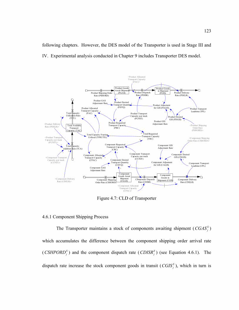
123

following chapters. However, the DES model of the Transporter is used in Stage III and

IV. Experimental analysis conducted in Chapter 9 includes Transporter DES model.

Product GoodsAwait Shipment

(PGAS)

Product Goodsin Shipment

(PGIS)Product Shipping OrderRate (PSHORD)

+Product DispatchRate (PDISR)

Product DeliveryRate (PDELR)

Product RequestedTransport Capacity

(PRC)

Product DesiredTransport Quantity

(PDTQ)Product Adjusmentfor GIS (PAGIS)

Product DesiredGIS (PDGIS)

Product AllocatedTransport Cap acity

(PAC)

Product TransportLeadtime (TPL)

Product TransportCapacity per truck

(PUNIT)Product GIS

Adjustment Rate

Product GASAdjustment Rate

-

+-

<Product ShippingOrder Rate

(PSHORD)>

+

+

+-

+

+

+-

Total RequestedTransport Capacity

(TRC)

Total AvailableTransport

Capacity (TAC)

Total CapacityAddition Rate (TCA)

Total CapacityUtilization Rate

(TCU)

+Total Capacity FractionUtilized (TFRUTIL)

+ + +

<Product DeliveryRate (PDELR)>

<Product TransportCapacity per truck

(PUNIT)>- +

ComponentGoods Await

Shipment(CGAS)

ComponentGoods in

Shipment (CGIS)Component ShippingOrder Rate (CSHORD)

+Component DispatchRate (CDISR)

Component RequestedTransport Capacity

(CRC)

Component DesiredTransport Quantity

(CDTQ)Component Adjusment

for GIS (CAGIS)

Component DesiredGIS (CDGIS)

Component AllocatedTransport Capacity

(CPAC)Component Transport

Leadtime (CPL)

Component TransportCapacity per truck

(CUNIT)

Component GISAdjustment Rate

Component GASAdjustment Rate -

+-

+

+

+

+

-

-+

Component DeliveryRate (CDELR)+

<Component Shipp ingOrder Rate (CSHORD)>

+

+

+

<Component DeliveryRate (CDELR)>

<Component TransportCapacity per truck

(CUNIT)>

-+

<Product AllocatedTransport Capacity

(PAC)>

+

+

<Component AllocatedTransport Capacity

(CPAC)>

-

+

Figure 4.7: CLD of Transporter

4.6.1 Component Shipping Process

The Transporter maintains a stock of components awaiting shipment ( )

which accumulates the difference between the component shipping order arrival rate

( ) and the component dispatch rate ( ) (see Equation 4.6.1). The

dispatch rate increase the stock component goods in transit ( ), which in turn is

SjCGAS

SjCSHPORD S

jCDISR

SjCGIS

124

reduced by the component delivery rate ( ) (see Equation 4.6.2). The shipment

of component goods is modeled as a pipeline delay, where the component delivery rate is

set equal to the component dispatch rate offset by a fixed lead time ( ) (see Equation

4.6.3).

SjCDELR

SjTCL

(4.6.1) [ ] /S Sj jtd CGAS dt CSHPORD CDISR= − S

jt

Sjt

S

S

(4.6.2) [ ] /S Sj jtd CGIS dt CDISR CDELR= −

(4.6.3) S Sjt jt TCLCDELR CDISR −=

The shipping process can begin only if there is sufficient transport capacity. That is,

component dispatch rate is constrained upon the available transport capacity. The

component dispatch rate is set equal to the allocated transport capacity (number of

trucks) times the capacity of a unit truck ( ) (see Equation 4.6.4). The allocated

capacity is captured as a function of the requested transport capacity ( ) and the

fraction transport capacity utilized (TFRUTIL ). The requested transport capacity reflects

the number of trucks required to transport the desired components ( ).

SjCAC

SjCUNIT

SjCRC

SjCDTQ

(4.6.4) S Sjt jt jCDISR CAC CUNIT= ⋅

(4.6.5) S Sjt jt tCAC CRC TFRUTIL= ⋅

(4.6.6) /S Sjt jt jCRC CDTQ CUNIT=

The Transporter determines the desired component transport quantities using a

variant of the production ordering rule, based upon the current component goods awaiting

125

shipment and the different between the desired levels of component goods in shipment

( ) and the current component goods in shipment (see Equation 4.6.7). The

fractional adjustment rate for (

SjCDGIS

SjCGAS CS

jλ ) describes how much of the current

component goods awaiting shipment are to be added to the desired transport quantities.

The fractional adjustment rate for (SjCGIS CS

jπ ) describes how much of the discrepancy

between the desired and current levels of component goods in shipment are to be added

to the desired transport quantities. Also, based on Little’s Law, the desired component

goods in shipment is set to yield the desired throughput, given the transport lead time

( ). SjTCL

(4.6.7) S CS Sjt j jt jtCDTQ CGAS CAGISλ= ⋅ + S

)

S

(4.6.8) (S CS S Sjt j jt jtCAGIS CDGIS CGISπ= ⋅ −

(4.6.9) S Sjt jt jtCDGIS CSHORD TCL= ⋅

4.6.2 Product Shipping Process

The process of shipping the product between the Manufacturer and the Retailers

can be described analogous to the component shipping process (refer Section 4.6.1).

Also, the determination of the desired product transport quantities is analogous to that of

the component (refer Section 4.6.1). The fractional adjustment rates of product awaiting

shipment ( PRiλ ) and product in shipment ( PR

iπ ) describes the rate at which the current

126

level of product awaiting shipment and the shortfall in the desired and current levels of

product in shipment is corrected, respectively.

(4.6.10) [ ] /R Ri itd PGAS dt PSHPORD PDISR= − R

it

Rit

R

R

R

R

R

(4.6.11) [ ] /R Ri itd PGIS dt PDISR PDELR= −

(4.6.12) Rit it TPLPDELR PDISR −=

(4.6.13) R Rit it iPDISR PAC PUNIT= ⋅

(4.6.14) R Rit it tPAC PRC TFRUTIL= ⋅

/ (4.6.15) R Rit it iPRC PDTQ PUNIT=

(4.6.16) R PR Rit j it itPDTQ PGAS PAGISλ= ⋅ +

( ) (4.6.17) R PR R Rit i it itPAGIS PDGIS PGISπ= ⋅ −

(4.6.18) R Rit it itPDGIS PSHORD TPL= ⋅

4.6.3 Transport Capacity Allocation

The Transporter maintains a stock of total available capacity ( ) which

accumulates the difference between the total capacity added (TCA ) and the total capacity

utilized (TC ). The total capacity added is defined as the sum of the capacity (trucks)

available immediately after the delivery of components and products. The total capacity

utilized is restricted by the total available capacity and the fraction of capacity utilized

(TFRUTIL ). The fraction capacity utilized is defined as a non-linear function of the total

TAC

U

127

requested capacity (TR ) and the total available capacity. The total requested capacity

is the sum of the requested transport capacity for all component and products.

C

[ ] / td TAC dt TCA TCUt= − (4.6.19)

(4.6.20) , ,

/S S Rt jt j it

j S i RTCA CDELR CUNIT PDELR PUNIT= +∑ ∑ / R

i

t t tTCU TAC TFRUTIL= ⋅ (4.6.21)

( /t tTFRUTIL f TRC TAC )t= (4.6.22)

, ,

St jt

j S i RTRC CRC PRC= + R

it∑ ∑ (4.6.23)

4.7 Calculation of Model Parameters for the Supply Chain Scenario

The generic system dynamic models for the Suppliers, Manufacturer and Retailers,

capable of handling multiple products and components are presented in Sections 4.3 – 4.6.

Based on the supply chain scenario, the following indices are set: Number of products, N

= 2; Number components, M = 2; Number of Suppliers, S = 2; and Number of Retailers,

R = 3.

At the Manufacturer, the key parameters of our interest includes the number of

stages of production ( MQ ) and the expected production lead time ( MiL ). This is

determined by building a comprehensive discrete-event model of the Manufacturer’s

shop, as per specifications in Section 3.5.3. This DES model of the Manufacturer’s shop

is simulated with a constant demand of 50 units/ week for each product (the demand is

modeled as a non-stationary Poisson process over the entire week), for 3 replications

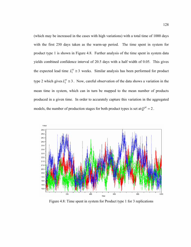
128

(which may be increased in the cases with high variations) with a total time of 1000 days

with the first 250 days taken as the warm-up period. The time spent in system for

product type 1 is shown in Figure 4.8. Further analysis of the time spent in system data

yields combined confidence interval of 20.5 days with a half width of 0.05. This gives

the expected lead time weeks. Similar analysis has been performed for product

type 2 which gives . Now, careful observation of the data shows a variation in the

mean time in system, which can in turn be mapped to the mean number of products

produced in a given time. In order to accurately capture this variation in the aggregated

models, the number of production stages for both product types is set at .

1 3ML ≅

2 3ML ≅

2MQ =

Figure 4.8: Time spent in system for Product type 1 for 3 replications

129

At the Suppliers, the key parameters of our interest includes the number of stages

of component production ( ) and the expected component production lead time ( ).

For Supplier 1, similar to the Manufacturer, a comprehensive discrete-event model of the

shop is built as per specifications in Section 3.5.4. This DES model of the Supplier 1’s

shop is simulated with a constant demand of 100 units/ week for component 1 (the

demand is modeled as a non-stationary Poisson process over the entire week), for 3

replications with a total time of 1000 days with the first 250 days taken as the warm-up

period. Analysis of the time spent in system data yields combined confidence interval of

14.1 days with a half width of 0.04. This gives the expected lead time weeks.

Again, in order to accurately capture the variation in component production rate, the

number of production stages is set at

SSQ SjSL

11 2SSL ≅

1 1SSQ = .

Supplier 2 is structured similar to the Manufacturer (see Section 3.5.4). Hence,

the parameters are maintained the same as used for the Manufacturer. That is, the

component production lead time 22 3SSL ≅ weeks and the number of production stages is

set at . 2 2SSQ =

Next, Transporter is modeled as per the specification in Section 3.5.5. This DES

model of the Transporter is simulated with a constant demand of 100 components/ week

from each Suppliers, 16 product_1s/ week to each Retailers and 16 product_2s/ week to

each Retailer (the demands are modeled as a non-stationary Poisson process over the

entire week), for 3 replications with a total time of 1000 days with the first 250 days

taken as the warm-up period. The observations of the transport time data yields the

130

values for the parameters, transportation component lead times weeks, and

transportation product lead times

2SjTCL ≅

2RiTPL ≅ weeks.

It is noted that the aggregated transportation lead times are used in the component

purchase ordering at the Manufacturer, and the collaborative inventory management.

Based on the analysis of the transportation system, the component supply lead time

weeks and the product delivery lead time1 2 2M MCL CL= ≅ 2MirLR ≅ weeks.

4.8 Chapter Summary

In this chapter, the aggregate-level system dynamic models used in the planning

stage (Stages I and II, see Figure 3.2) of the different members of the supply chain were

described. The models developed (specific contributions of this research) capture (1) the

mixing and variability in the production process and the production lead time, (2)

capacitated resource allocation, (3) order backlog, (4) frequency of information update,

(5) raw material component inventory, (6) transportation network, and (5) provides for

spatial and lateral dimension of the supply chain. Next, the models of individual

members of the supply chain have been defined conceptually using modified causal loop

diagrams (CLD), and differential equations.

131

CHAPTER 5

STABILITY ANALYSIS OF SUPPLY CHAIN PLANNING (STAGE I)

In this chapter, the conditions for stability of the supply chain are derived (relating

all parameters) and the effects of intra-player sampling interval and inter-player sampling

intervals have been analyzed. The conceptual models and differential equations

presented in Chapter 4 are first translated into difference equation models that can be

readily simulated and analyzed using function transformation technique (z-transform).

The discretization and linearization techniques employed, to enable analysis using z-

transform technique, are discussed. Backgrounds on the functional transformation

technique and z-transform method are presented in Sections 5.1 and 5.2.

The first part of the chapter (Section 5.3) focuses on the production ordering and

inventory control module of the supply chain models. The transfer functions are obtained

and conditions of the stability (settings of control parameters that produce stable

responses) are derived. The variation in the stability of the system operating under

sufficient inventory coverage and the stability of the system operating under limited

inventory coverage are highlighted. The effects of the frequency of information update

(intra-player sampling interval) on the stability are examined by relating the update

frequency to the sampling interval of the underlying difference equations. Guidance for

the selection of appropriate parameters depending on the ordering characteristics of firms

to guarantee system stability is presented.

132

The second part of the chapter (Section 5.4) focuses on the supply chain models’

interactions. The variation in the stability of the supply chain operating under

collaborative configuration is highlighted. The effects of the frequency of information

update (inter-player sampling interval) between the different players on the stability are

examined. Guidance for the selection of appropriate parameters depending on the supply

chain characteristics to guarantee stability is presented.

Existence of instability due to the improper parameter selection and improper

sampling interval selection is thus confirmed, and guidance for the selection of

appropriate parameters depending on the ordering characteristics of firms to guarantee

system stability is presented. System dynamic simulations are used to confirm the

analysis and help demonstrate the stable or unstable behavior of the supply chain system.

5.1 Function Transformation Technique for System Analysis

Past research work have been presented (see Chapter 2) in which supply chain or

production-inventory control systems are captured using feedback-based structures

(Forrester 1961, Towill 1982, Axsäter 1985, Edghill and Towill 1990, Sterman 2000) and

analyzed through the application of control theoretic tools such as block diagram algebra,

Bode plots, and functional transformations (Wikner et al. 1992, John et al. 1994,

Grubbström and Wikner 1996, Disney and Towill 2002, Disney et al. 2004). In this

research work, modified causal loop diagrams are used to capture the production and

purchase ordering and the inventory management at the Manufacturer, Suppliers and

Retailers (see Chapter 4). In this chapter, these models are analyzed by applying z-

133

transformation technique (a type of function transformation technique). The discrete

nature the planning problem (i.e. planning is typically done with a time period of 1 week

or 1 day) prompted the use of z-transform technique. Function transformation technique

maps the system from the time domain to the frequency domain; the advantages of which

are summarized below (Disney and Towill 2002):

• Frequency response analysis has been found to be an efficient tool to examine the

critical design parameters and identify ranges of parameter values that give good

transient response performance (Ortega and Lin 2004),

• Standard techniques exists to analyze the system performance such as rise time, peak

overshoots, and settling time, without recourse to simulation (Bissell 1996),

• Frequency domain calculations can be computationally very simple (Bissell 1996),

• Closed loop transfer functions of the system can be obtained that enables to gain

insight into the stability of the system,

• Appropriate integration of transfer functions with simulation enables additional

system analysis (Disney and Towill 2002),

• A number of techniques exist for transferring problems from one domain (Laplace, z,

Fourier, w, frequency, etc) to another domain, to help gain insight from situations that

have already been encountered and solved in other domains (Disney and Towill 2002),

• Transforms can be used to capture the stochastic properties by serving as moment

generating functions (Grubbström 1998).

134

A comprehensive literature review on the use of control theoretic concepts for the

dynamic analysis of supply chains and production – inventory systems have been

presented in Chapter 2.

5.2 Overview of Stability Analysis using z-Transform Technique

The z-transform technique is applicable for the functional transformation of

sequences. In sampled systems, a continuous function f(s) can be represented as a

sequence of values ( ),

: ( ) :t s tf f t f s

δ= where t = 0, 1, 2 ... and δ > 0 is known as the

discretization step or sampling interval. The one-sided z-transform of the sequence ( )f t

is defined as:

0

[ ( )] [ ] ( ) t

tZ f t F z f t z

∞−

=

= =∑

The polynomials in the numerator and denominator of can be factored, and

can be written in terms of those factors as shown below.

[ ]F z [ ]F z

1 2

1 2

( )( )...( )[ ][ ][ ] ( )( )...( )

m

n

z z z z z zN zF z GD z z p z p z p

− − −= =

− − −

where, G is the gain factor and s are the zeros and the iz ip s are the poles. The zeros are

the roots of the numerator polynomial, and the poles are the roots of the denominator

polynomial. Thus, the transfer function has m finite zeros and n finite poles. Also,

there will be

[ ]F z

n m− zeros (if n > m), or poles (if n < m) at the origin . These poles

and zeros are either real or appear in complex conjugate pairs. A pole-zero plot of a z-

0z =

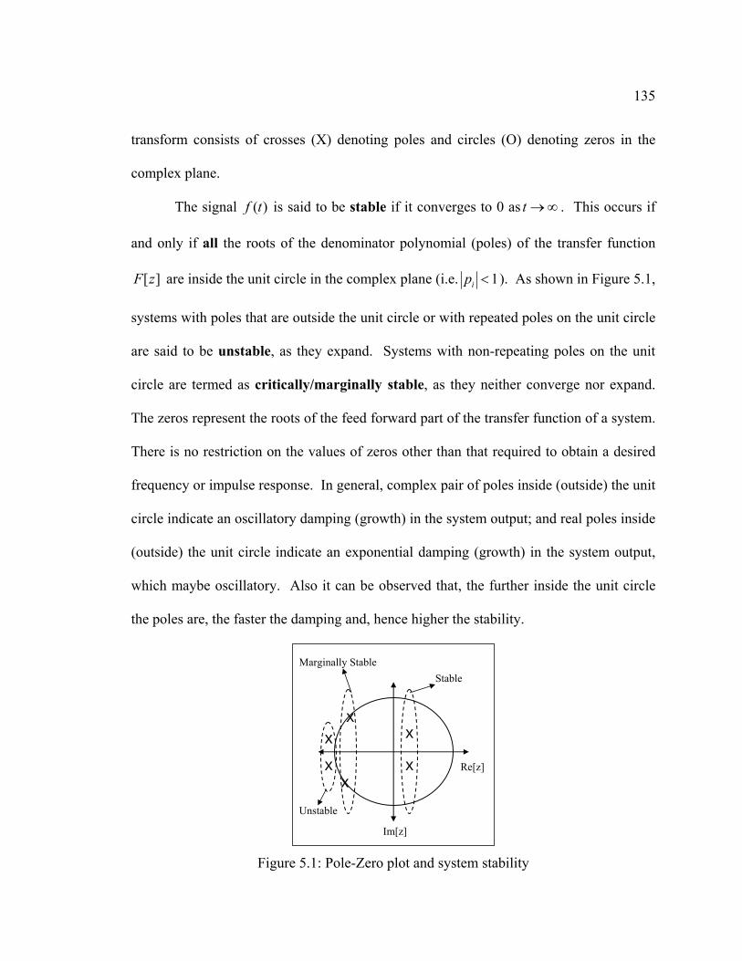
135

transform consists of crosses (X) denoting poles and circles (O) denoting zeros in the

complex plane.

The signal ( )f t is said to be stable if it converges to 0 as . This occurs if

and only if all the roots of the denominator polynomial (poles) of the transfer function

are inside the unit circle in the complex plane (i.e.

t →∞

[ ]F z 1ip < ). As shown in Figure 5.1,

systems with poles that are outside the unit circle or with repeated poles on the unit circle

are said to be unstable, as they expand. Systems with non-repeating poles on the unit

circle are termed as critically/marginally stable, as they neither converge nor expand.

The zeros represent the roots of the feed forward part of the transfer function of a system.

There is no restriction on the values of zeros other than that required to obtain a desired

frequency or impulse response. In general, complex pair of poles inside (outside) the unit

circle indicate an oscillatory damping (growth) in the system output; and real poles inside

(outside) the unit circle indicate an exponential damping (growth) in the system output,

which maybe oscillatory. Also it can be observed that, the further inside the unit circle

the poles are, the faster the damping and, hence higher the stability.

Im[z]

Re[z]

x

x

x

x

xx

StableMarginally Stable

Unstable

Figure 5.1: Pole-Zero plot and system stability

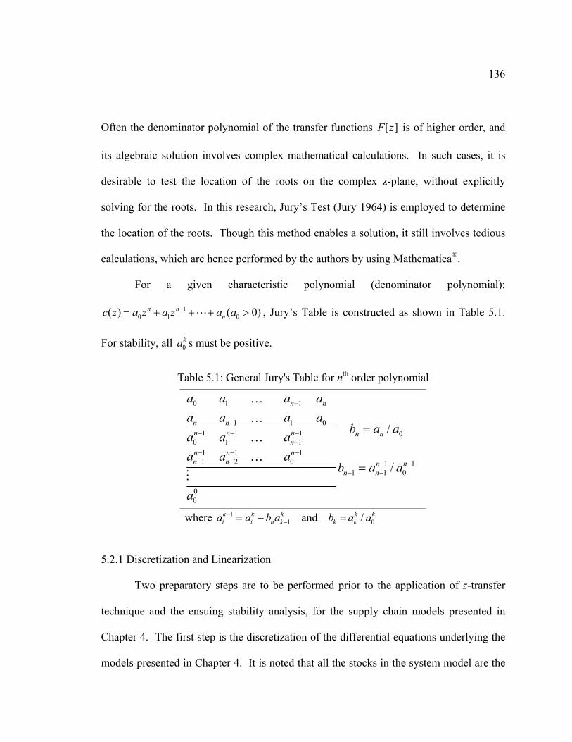
136

Often the denominator polynomial of the transfer functions is of higher order, and

its algebraic solution involves complex mathematical calculations. In such cases, it is

desirable to test the location of the roots on the complex z-plane, without explicitly

solving for the roots. In this research, Jury’s Test (Jury 1964) is employed to determine

the location of the roots. Though this method enables a solution, it still involves tedious

calculations, which are hence performed by the authors by using Mathematica

[ ]F z

®.

For a given characteristic polynomial (denominator polynomial):

, Jury’s Table is constructed as shown in Table 5.1.

For stability, all s must be positive.

10 1 0( ) ( 0)n n

nc z a z a z a a−= + + + >

0ka

Table 5.1: General Jury's Table for nth order polynomial

0 1 1

1 1 01 1 1 0

0 1 11 1 11 2 0 1 1

1 1 0

00

/

/

n n

n nn n n n n

nn n nn n n n

n n

a a a aa a a a

b a aa a aa a a

b a a

a

−

−− − −

−− − −− − − −

− −

=

=

…………

where 11 0and /k k k k

i i n k k ka a b a b a a−−= − = k

5.2.1 Discretization and Linearization

Two preparatory steps are to be performed prior to the application of z-transfer

technique and the ensuing stability analysis, for the supply chain models presented in

Chapter 4. The first step is the discretization of the differential equations underlying the

models presented in Chapter 4. It is noted that all the stocks in the system model are the

137

only equations defined as the differential equations, to reflect the accumulation of the

stock over time. Accordingly, the differential equations of the stock are discretized, with

a sampling interval of δ, as follows:

1 n[Stock]/ Inflow( ) Outflow( ) Stock Stock (Inflow Outflow )n nd dt t t nδ−= − ⇒ = + ⋅ −

The sampling interval (δ) is said to correspond with the frequency at which the

information is updated within the system. Typically, in the past research works

(Grubbström 1998, Disney and Towill 2002), the sampling interval δ is implicitly

assumed to be equal to 1, indicating a weekly update of the ordering rule. In the current

research work, the impact of the frequency of information update on the dynamics of the

system is explicitly measured. It is noted that the sampling interval δ refers to the

planning and execution frequency.

The second step prior to the z-transform analysis is the linearization of the non-

linear functions present in the system models. Linearization is important as the exact

solution using z-transform analysis can be obtained only for a linear system, which can

serve as approximate solutions to the non-linear models. The non-linear functions are

found to arise in the supply chain models due to ‘saturation effect’. The saturation effect

results in sharp discontinuities in the output in response to varying input. In the models,

the shipment rates, the production rates and purchase order rates are the typical non-linear

functions characterized by the saturation effect. In this research, such non-linear

functions are linearized using local linearization technique, in which the non-linear

function is separated into piecewise linear functions.

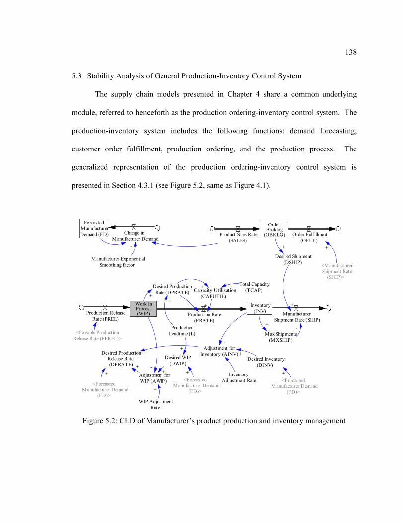
138

5.3 Stability Analysis of General Production-Inventory Control System

The supply chain models presented in Chapter 4 share a common underlying

module, referred to henceforth as the production ordering-inventory control system. The

production-inventory system includes the following functions: demand forecasting,

customer order fulfillment, production ordering, and the production process. The

generalized representation of the production ordering-inventory control system is

presented in Section 4.3.1 (see Figure 5.2, same as Figure 4.1).

Work InProcess(WIP)

Inventory(INV)Production Rate

(PRATE)Production Release

Rate (PREL)Manufacturer

Shipment Rate (SHIP)

Max Shipments(MXSHIP)

-+





Desired WIP(DWIP)

-+

-

+

+

+

WIP AdjustmentRate

+

InventoryAdjustment Rate

+

ProductionLeadtime (L)

+

<Feasible ProductionRelease Rate (FPREL)>

Desired Product ionRate (DPRATE)+

-

+

Total Capacity(TCAP)Capacity Utilizat ion

(CAPUTIL)

+

+

ForcastedManufacturerDemand (FD) Change in

Manufacturer Demand

Manufacturer ExponentialSmoothing factor

--


(FD)>


(FD)><Forcasted


+ + +

OrderBacklog

(OBKLG)Product Sales Rate(SALES)

Order Fulfillment(OFUL)

<ManufacturerShipment Rate

(SHIP)>

+

Desired Shipment(DSHIP)

++

+

Figure 5.2: CLD of Manufacturer’s product production and inventory management

139

Figure 5.2 illustrates the Manufacturer’s product production and inventory control

system. Manufacturer’s component order management (see Section 4.3.2) and Supplier

component production and inventory management (see Section 4.5.1) can be obtained as

special cases of this production ordering-inventory control system, as shown below:

• Manufacturer’s component order management (see Section 4.3.2): This model can be

obtained by mapping (from Figure 5.1 to Figure 4.3), the (1) product WIP to

component GIT, (2) product inventory to component inventory, (3) product

production lead time to component supply lead time, (4) desired production usage

rate to product sales rate, (5) forecasted product demand to desired component usage

rate, (6) exponential smoothing constant of product is set to 1, and (7) order backlogs

are removed.

• Supplier’s component production and inventory management (see Section 4.5.1):

This model can be obtained by direct mapping (from Figure 5.1 to Figure 4.6).

Hence, it is important and essential to analyze the stability of the general

production ordering and inventory control system, as (1) it is applicable to different parts

of the supply chain, and (2) it helps understand the dynamics of the production ordering

and inventory control system of the individual players in response to all their external

inputs.

In this section, the model presented in Section 4.3.1 will be analyzed using z-

transform technique. In past literature, ordering and inventory based production control

systems have been analyzed using the z-transform technique (Vassain 1954, Adelson

1966, Deziel and Eilon 1967, Boney et al. 1994, Grubbström 1998, Disney and Towill

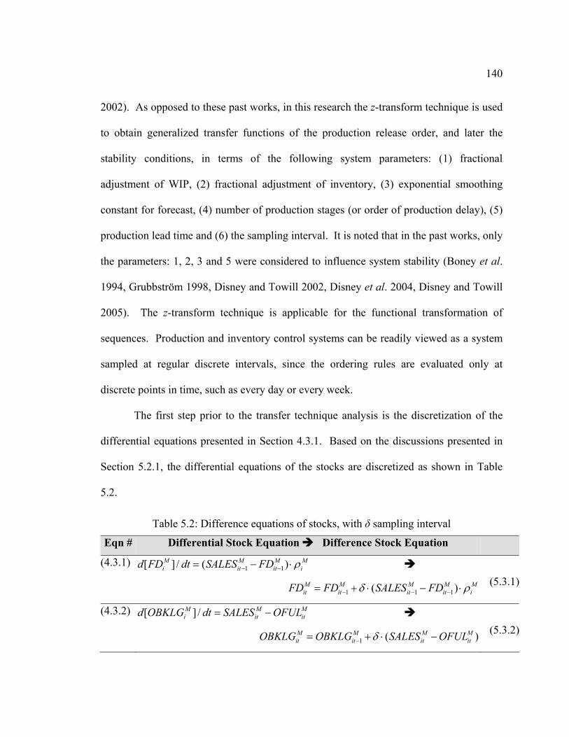
140

2002). As opposed to these past works, in this research the z-transform technique is used

to obtain generalized transfer functions of the production release order, and later the

stability conditions, in terms of the following system parameters: (1) fractional

adjustment of WIP, (2) fractional adjustment of inventory, (3) exponential smoothing

constant for forecast, (4) number of production stages (or order of production delay), (5)

production lead time and (6) the sampling interval. It is noted that in the past works, only

the parameters: 1, 2, 3 and 5 were considered to influence system stability (Boney et al.

1994, Grubbström 1998, Disney and Towill 2002, Disney et al. 2004, Disney and Towill

2005). The z-transform technique is applicable for the functional transformation of

sequences. Production and inventory control systems can be readily viewed as a system

sampled at regular discrete intervals, since the ordering rules are evaluated only at

discrete points in time, such as every day or every week.

The first step prior to the transfer technique analysis is the discretization of the

differential equations presented in Section 4.3.1. Based on the discussions presented in

Section 5.2.1, the differential equations of the stocks are discretized as shown in Table

5.2.

Table 5.2: Difference equations of stocks, with δ sampling interval

Eqn # Differential Stock Equation Difference Stock Equation

(4.3.1) 1 1[ ] / ( )M M M M

i it it id FD dt SALES FD ρ− −= − ⋅

1

1 1( )M M M Mit it it it iFD FD SALES FD Mδ ρ− − −= + ⋅ − ⋅ (5.3.1)

(4.3.2) [ ] /M Mi itd OBKLG dt SALES OFUL= − M

it

M

1 ( )M M Mit it it itOBKLG OBKLG SALES OFULδ−= + ⋅ − (5.3.2)

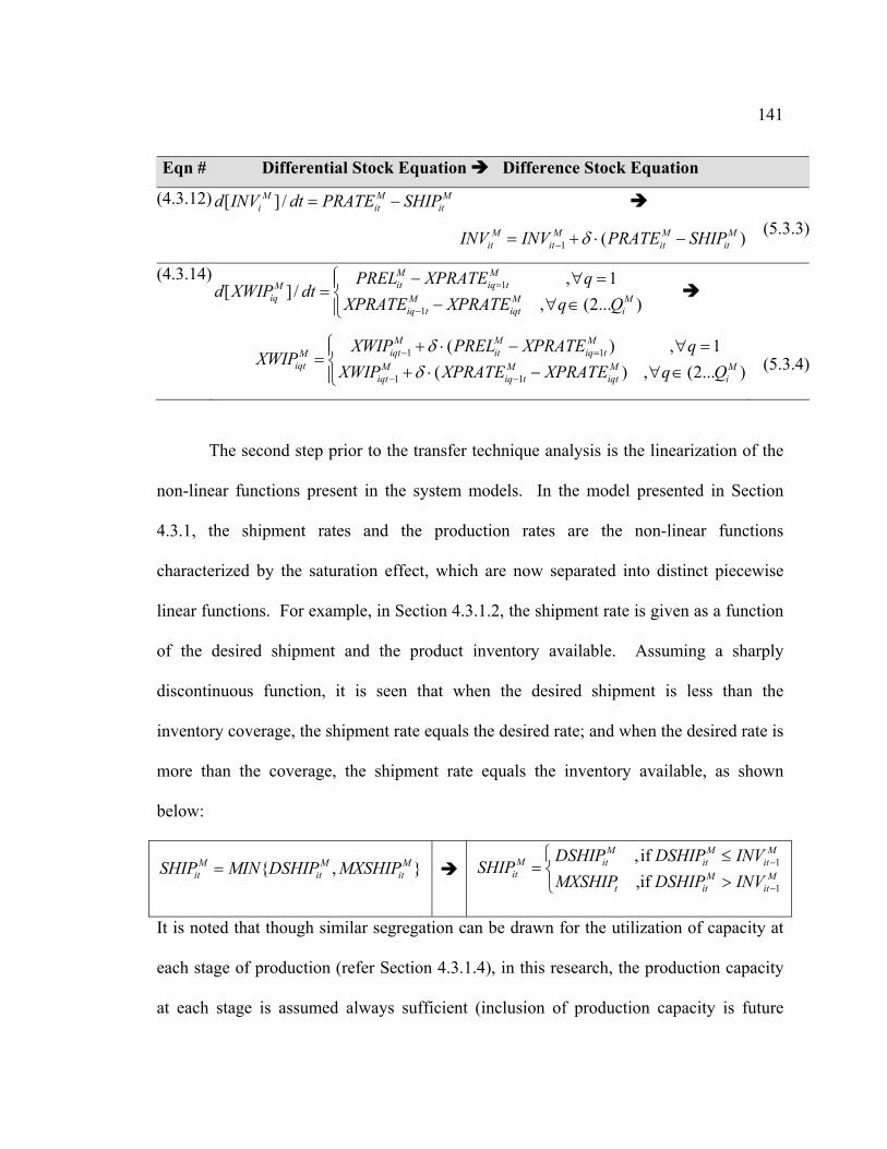
141


(4.3.12) [ ] /M M Mi it itINV dt PRATE SHIP= −

M

d

1 ( )M M Mit it it itINV INV PRATE SHIPδ−= + ⋅ − (5.3.3)

(4.3.14)1

1

, 1[ ] /

, (2... )

M Mit iq tM

iq M Miq t iqt i

PREL XPRATE qd XWIP dt MXPRATE XPRATE q Q

=

−

⎧ − ∀⎪= ⎨ − ∀ ∈⎪⎩

=

1M

1 1

1 1

( ) ,( ) , (2... )

M M Miqt it iq tM

iqt M M Miqt iq t iqt i

XWIP PREL XPRATE qXWIP

XWIP XPRATE XPRATE q Qδ

δ− =

− −

⎧ + ⋅ − ∀ =⎪= ⎨ + ⋅ − ∀ ∈⎪⎩(5.3.4)

The second step prior to the transfer technique analysis is the linearization of the

non-linear functions present in the system models. In the model presented in Section

4.3.1, the shipment rates and the production rates are the non-linear functions

characterized by the saturation effect, which are now separated into distinct piecewise

linear functions. For example, in Section 4.3.1.2, the shipment rate is given as a function

of the desired shipment and the product inventory available. Assuming a sharply

discontinuous function, it is seen that when the desired shipment is less than the

inventory coverage, the shipment rate equals the desired rate; and when the desired rate is

more than the coverage, the shipment rate equals the inventory available, as shown

below:

{ ,M Mit it itSHIP MIN DSHIP MXSHIP= }M 1

1

, if ,if

M M MM it it it

it M Mt it

DSHIP DSHIP INVSHIP

itMXSHIP DSHIP INV−

−

⎧ ≤= ⎨

>⎩

It is noted that though similar segregation can be drawn for the utilization of capacity at

each stage of production (refer Section 4.3.1.4), in this research, the production capacity

at each stage is assumed always sufficient (inclusion of production capacity is future

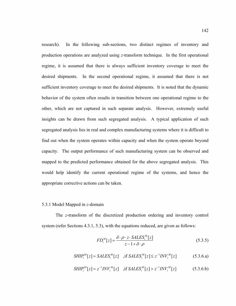
142

research). In the following sub-sections, two distinct regimes of inventory and

production operations are analyzed using z-transform technique. In the first operational

regime, it is assumed that there is always sufficient inventory coverage to meet the

desired shipments. In the second operational regime, it assumed that there is not

sufficient inventory coverage to meet the desired shipments. It is noted that the dynamic

behavior of the system often results in transition between one operational regime to the

other, which are not captured in such separate analysis. However, extremely useful

insights can be drawn from such segregated analysis. A typical application of such

segregated analysis lies in real and complex manufacturing systems where it is difficult to

find out when the system operates within capacity and when the system operate beyond

capacity. The output performance of such manufacturing system can be observed and

mapped to the predicted performance obtained for the above segregated analysis. This

would help identify the current operational regime of the systems, and hence the

appropriate corrective actions can be taken.

5.3.1 Model Mapped in z-domain

The z-transform of the discretized production ordering and inventory control

system (refer Sections 4.3.1, 5.3), with the equations reduced, are given as follows:

[ ][ ]1

MM ii

z SALES zFD zz

δ ρδ ρ

⋅ ⋅ ⋅=

− + ⋅ (5.3.5)

(5.3.6.a) 1[ ] [ ] , if [ ] [ ]M M Mi i iSHIP z SALES z SALES z z INV z−= M

i≤

1 Mi

−> (5.3.6.b) 1[ ] [ ] ,if [ ] [ ]M M Mi i iSHIP z z INV z SALES z z INV z−=

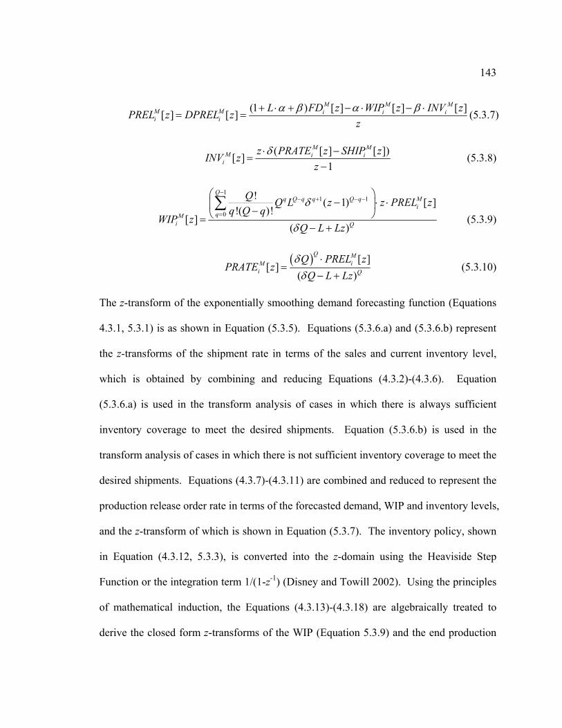
143

(1 ) [ ] [ ] [ ][ ] [ ]M M

M M i ii i

L FD z WIP z INVPREL z DPREL zz

α β α β+ ⋅ + − ⋅ − ⋅= =

Mi z (5.3.7)

( [ ] [[ ]1

M MM i i

iz PRATE z SHIP zINV z

zδ⋅ −

=−

]) (5.3.8)

11 1

0

! ( 1) [!( )!

[ ]( )

Qq Q q q Q q M

iqM

i Q

Q Q L z z PREL zq Q q

WIP zQ L Lz

δ

δ

−− + − −

=

⎛ ⎞− ⋅ ⋅⎜ ⎟−⎝ ⎠=

− +

∑ ] (5.3.9)

( ) [ ][ ]

( )

Q MiM

i Q

Q PREL zPRATE z

Q L Lzδδ

⋅=

− + (5.3.10)

The z-transform of the exponentially smoothing demand forecasting function (Equations

4.3.1, 5.3.1) is as shown in Equation (5.3.5). Equations (5.3.6.a) and (5.3.6.b) represent

the z-transforms of the shipment rate in terms of the sales and current inventory level,

which is obtained by combining and reducing Equations (4.3.2)-(4.3.6). Equation

(5.3.6.a) is used in the transform analysis of cases in which there is always sufficient

inventory coverage to meet the desired shipments. Equation (5.3.6.b) is used in the

transform analysis of cases in which there is not sufficient inventory coverage to meet the

desired shipments. Equations (4.3.7)-(4.3.11) are combined and reduced to represent the

production release order rate in terms of the forecasted demand, WIP and inventory levels,

and the z-transform of which is shown in Equation (5.3.7). The inventory policy, shown

in Equation (4.3.12, 5.3.3), is converted into the z-domain using the Heaviside Step

Function or the integration term 1/(1-z-1) (Disney and Towill 2002). Using the principles

of mathematical induction, the Equations (4.3.13)-(4.3.18) are algebraically treated to

derive the closed form z-transforms of the WIP (Equation 5.3.9) and the end production

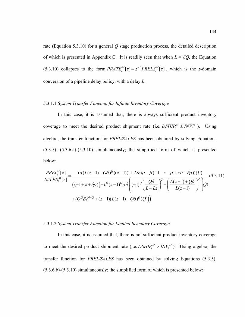
144

rate (Equation 5.3.10) for a general Q stage production process, the detailed description

of which is presented in Appendix C. It is readily seen that when L = δQ, the Equation

(5.3.10) collapses to the form , which is the z-domain

conversion of a pipeline delay policy, with a delay L.

[ ] [ ]M L MiPRATE z z PRELS z−= i

5.3.1.1 System Transfer Function for Infinite Inventory Coverage

In this case, it is assumed that, there is always sufficient product inventory

coverage to meet the desired product shipment rate (i.e. M MiDSHIP INV≤ i ). Using

algebra, the transfer function for PREL/SALES has been obtained by solving Equations

(5.3.5), (5.3.6.a)-(5.3.10) simultaneously; the simplified form of which is presented

below:

( (

))1

[ ] ( ( ( 1) ) (( 1)(1 ) ( 1 )) !)[ ] ( 1)( 1 ) ( 1) ( 1) !

( 1)

( ( 1)( ( 1) ) ) !

M QiM QQi Q Q Q

Q Q Q

PREL z L z Q z L z z QSALES z Q L z Qz L z

L Lz L z

Q z L z Q Q

δ δ α ρ β ρ ρ δρ

δ δδρ αδ

βδ δ+

− + − + + − + − + +=

⎛ ⎞⎛ ⎞− +⎛ ⎞⎜ ⎟− + + − − − −⎜ ⎟ ⎜ ⎟ ⎟⎜ − −⎝ ⎠ ⎝ ⎠ ⎠⎝

+ + − − +

Q

(5.3.11)

5.3.1.2 System Transfer Function for Limited Inventory Coverage

In this case, it is assumed that, there is not sufficient product inventory coverage

to meet the desired product shipment rate (i.e. M MiDSHIP INV> i ). Using algebra, the

transfer function for PREL/SALES has been obtained by solving Equations (5.3.5),

(5.3.6.b)-(5.3.10) simultaneously; the simplified form of which is presented below:

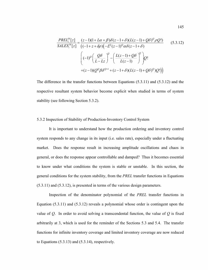
145

( (

))1

[ ] ( 1)(1 ) ( 1 )( ( 1) ) !)[ ] ( 1 ) ( 1) ( 1 )

( 1)( 1) !( 1)

( 1)( ( 1 )( ( 1) ) ) !

M QiM Q Qi

QQQ

Q Q Q

PREL z z L z L z Q QSALES z z L z z

Q L z Q QL Lz L z

z Q z L z Q Q

α β δ δ δ ρδρ αδ δ

δ δ

βδ δ δ+

− + + − + − +=

− + + − − − +

⎛ ⎞⎛ ⎞− +⎛ ⎞⎜ ⎟− −⎜ ⎟ ⎜ ⎟ ⎟⎜ − −⎝ ⎠ ⎝ ⎠ ⎠⎝

+ − + − + − +

(5.3.12)

The difference in the transfer functions between Equations (5.3.11) and (5.3.12) and the

respective resultant system behavior become explicit when studied in terms of system

stability (see following Section 5.3.2).

5.3.2 Inspection of Stability of Production-Inventory Control System

It is important to understand how the production ordering and inventory control

system responds to any change in its input (i.e. sales rate), especially under a fluctuating

market. Does the response result in increasing amplitude oscillations and chaos in

general, or does the response appear controllable and damped? Thus it becomes essential

to know under what conditions the system is stable or unstable. In this section, the

general conditions for the system stability, from the PREL transfer functions in Equations

(5.3.11) and (5.3.12), is presented in terms of the various design parameters.

Inspection of the denominator polynomial of the PREL transfer functions in

Equation (5.3.11) and (5.3.12) reveals a polynomial whose order is contingent upon the

value of Q. In order to avoid solving a transcendental function, the value of Q is fixed

arbitrarily at 3, which is used for the reminder of the Sections 5.3 and 5.4. The transfer

functions for infinite inventory coverage and limited inventory coverage are now reduced

to Equations (5.3.13) and (5.3.14), respectively.

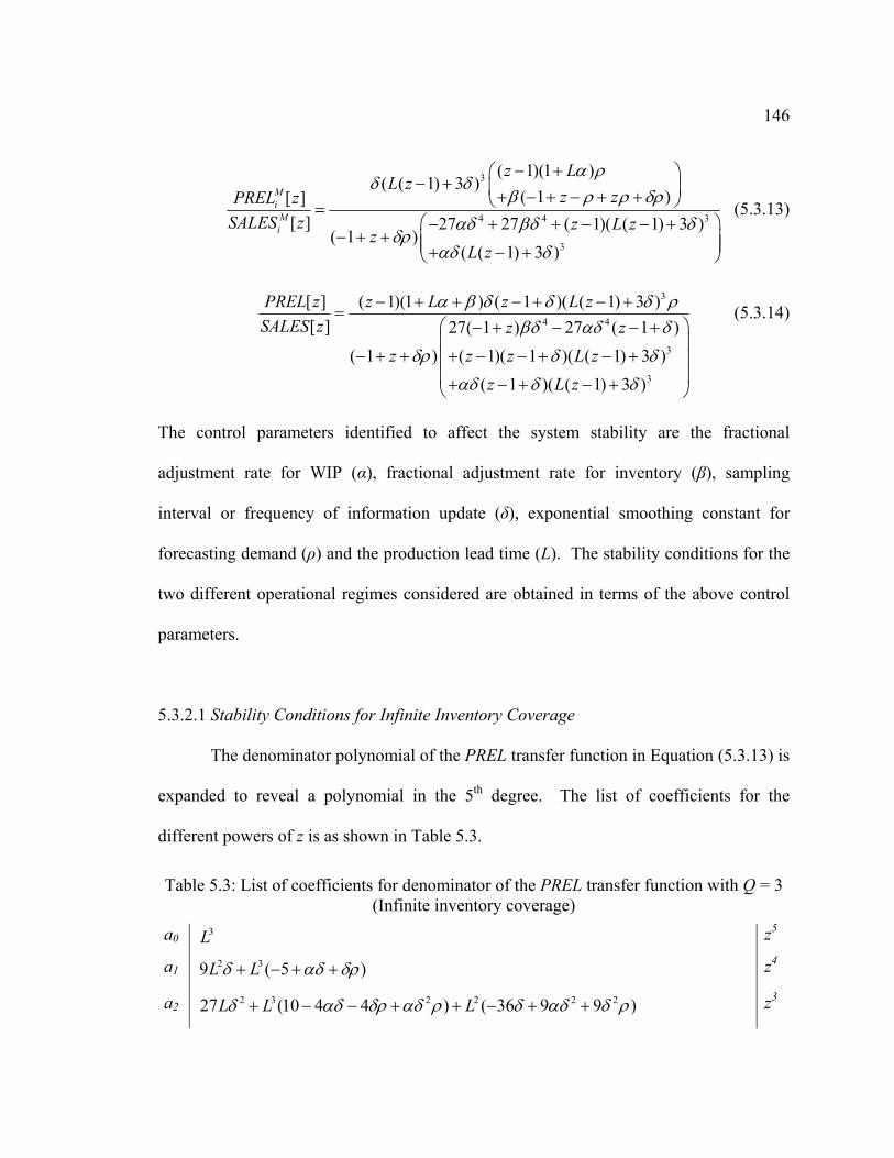
146

3

4 4

3

( 1)(1 )( ( 1) 3 )

( 1 )[ ][ ] 27 27 ( 1)( ( 1) 3 )

( 1 )( ( 1) 3 )

MiMi

z LL z

z zPREL zSALES z z L z

zL z

α ρδ δ

β ρ ρ δραδ βδ δ

δραδ δ

− +⎛ ⎞− + ⎜ ⎟+ − + − + +⎝ ⎠=⎛ ⎞− + + − − +

− + + ⎜ ⎟⎜ ⎟+ − +⎝ ⎠

3 (5.3.13)

3

4 4

3

3

[ ] ( 1)(1 ) ( 1 )( ( 1) 3 )[ ] 27( 1 ) 27 ( 1 )

( 1 ) ( 1)( 1 )( ( 1) 3 )( 1 )( ( 1) 3 )

PREL z z L z L zSALES z z z

z z z L zz L z

α β δ δ δ ρβδ αδ δ

δρ δ δ

αδ δ δ

− + + − + − +=

⎛ ⎞− + − − +⎜ ⎟

− + + + − − + − +⎜ ⎟⎜ ⎟+ − + − +⎝ ⎠

(5.3.14)

The control parameters identified to affect the system stability are the fractional

adjustment rate for WIP (α), fractional adjustment rate for inventory (β), sampling

interval or frequency of information update (δ), exponential smoothing constant for

forecasting demand (ρ) and the production lead time (L). The stability conditions for the

two different operational regimes considered are obtained in terms of the above control

parameters.

5.3.2.1 Stability Conditions for Infinite Inventory Coverage

The denominator polynomial of the PREL transfer function in Equation (5.3.13) is

expanded to reveal a polynomial in the 5th degree. The list of coefficients for the

different powers of z is as shown in Table 5.3.

Table 5.3: List of coefficients for denominator of the PREL transfer function with Q = 3 (Infinite inventory coverage)

a0 3L z5

a1 2 39 ( 5L L )δ αδ δρ+ − + + z4

a2 2 3 2 2 2 227 (10 4 4 ) ( 36 9 9 )L L Lδ αδ δρ αδ ρ δ αδ δ ρ+ − − + + − + + z3

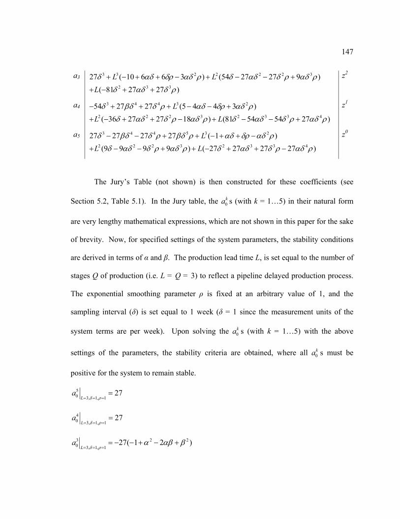
147

a3 3 3 2 2 2 2 3

2 3 3

27 ( 10 6 6 3 ) (54 27 27 9 )( 81 27 27 )

L LLδ αδ δρ αδ ρ δ αδ δ ρ αδ ρ

δ αδ δ ρ

+ − + + − + − − +

+ − + +

z2

a4 3 4 4 3 2

2 2 2 3 2 3 3

54 27 27 (5 4 4 3 )( 36 27 27 18 ) (81 54 54 27 )

LL Lδ βδ δ ρ αδ δρ αδ ρ

4δ αδ δ ρ αδ ρ δ αδ δ ρ αδ ρ

− + + + − − +

+ − + + − + − − +

z1

a5 3 4 4 5 3 2

2 2 2 3 2 3 3

27 27 27 27 ( 1 )(9 9 9 9 ) ( 27 27 27 27 )

LL Lδ βδ δ ρ βδ ρ αδ δρ αδ ρ

4δ αδ δ ρ αδ ρ δ αδ δ ρ αδ ρ

− − + + − + + −

+ − − + + − + + −

z0

The Jury’s Table (not shown) is then constructed for these coefficients (see

Section 5.2, Table 5.1). In the Jury table, the s (with k = 1…5) in their natural form

are very lengthy mathematical expressions, which are not shown in this paper for the sake

of brevity. Now, for specified settings of the system parameters, the stability conditions

are derived in terms of α and β. The production lead time L, is set equal to the number of

stages Q of production (i.e. L = Q = 3) to reflect a pipeline delayed production process.

The exponential smoothing parameter ρ is fixed at an arbitrary value of 1, and the

sampling interval (δ) is set equal to 1 week (δ = 1 since the measurement units of the

system terms are per week). Upon solving the s (with k = 1…5) with the above

settings of the parameters, the stability criteria are obtained, where all s must be

positive for the system to remain stable.

0ka

0ka

0ka

50 3, 1, 1

27L

aδ ρ= = =

=

40 3, 1, 1

27L

aδ ρ= = =

=

3 20 3, 1, 1

27( 1 2 )L

aδ ρ

2α αβ β= = =

= − − + − +

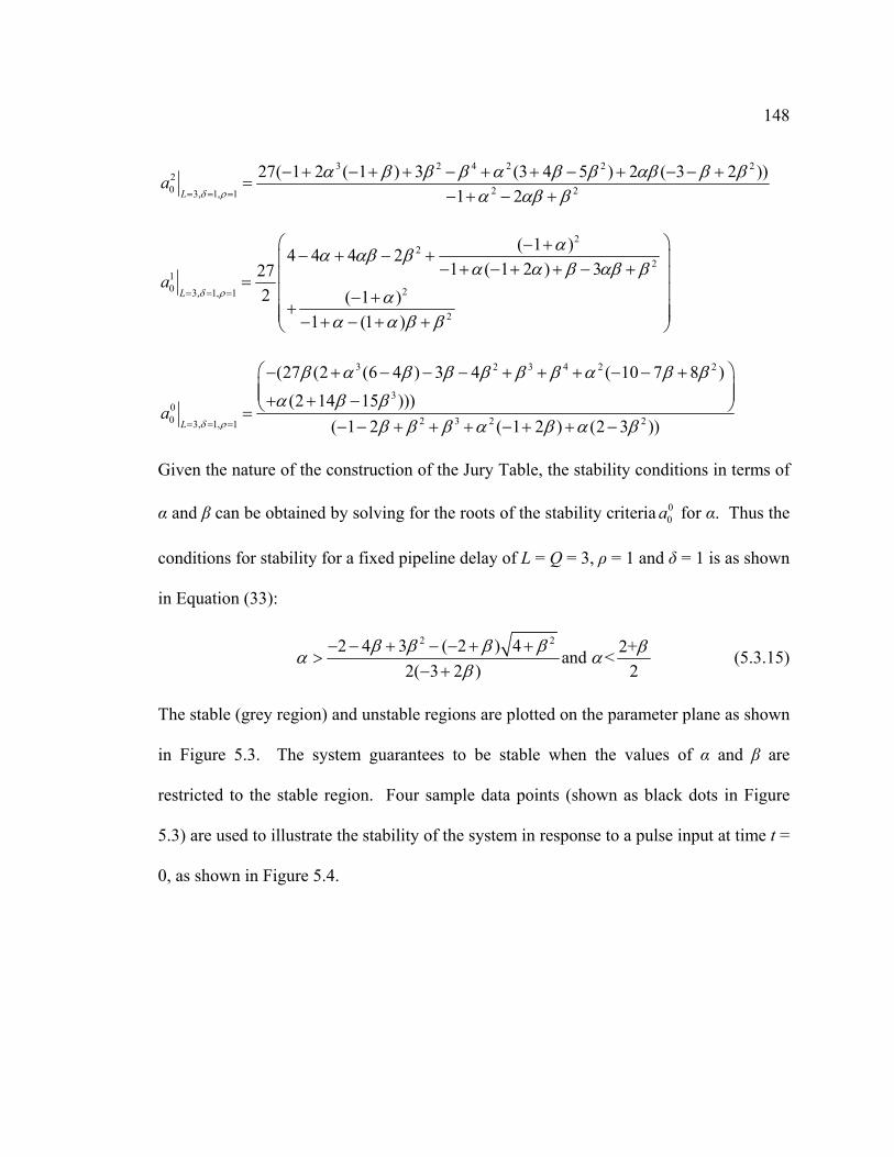
148

3 2 4 2 220 2 23, 1, 1

27( 1 2 ( 1 ) 3 (3 4 5 ) 2 ( 3 2 ))1 2L

aδ ρ

α β β β α β β αβ β βα αβ β= = =

− + − + + − + + − + − − +=

− + − +

2

22

210 23, 1, 1

2

( 1 )4 4 4 21 ( 1 2 ) 327

2 ( 1 )1 (1 )

La

δ ρ

αα αβ βα α β αβ β

αα α β β

= = =

⎛ ⎞− +− + − +⎜ ⎟− + − + + − +⎜ ⎟=

⎜ ⎟− ++⎜ ⎟⎜ ⎟− + − + +⎝ ⎠

3 2 3 4 2 2

300 2 3 2 23, 1, 1

(27 (2 (6 4 ) 3 4 ( 10 7 8 )(2 14 15 )))

( 1 2 ( 1 2 ) (2 3 ))La

δ ρ

β α β β β β β α β β

α β ββ β β α β α β= = =

⎛ ⎞− + − − − + + + − − +⎜ ⎟⎜ ⎟+ + −⎝ ⎠=

− − + + + − + + −

Given the nature of the construction of the Jury Table, the stability conditions in terms of

α and β can be obtained by solving for the roots of the stability criteria for α. Thus the

conditions for stability for a fixed pipeline delay of L = Q = 3, ρ = 1 and δ = 1 is as shown

in Equation (33):

00a

2 22 4 3 ( 2 ) 4 2+and <

2( 3 2 ) 2β β β β βα α

β− − + − − + +

>− +

(5.3.15)

The stable (grey region) and unstable regions are plotted on the parameter plane as shown

in Figure 5.3. The system guarantees to be stable when the values of α and β are

restricted to the stable region. Four sample data points (shown as black dots in Figure

5.3) are used to illustrate the stability of the system in response to a pulse input at time t =

0, as shown in Figure 5.4.

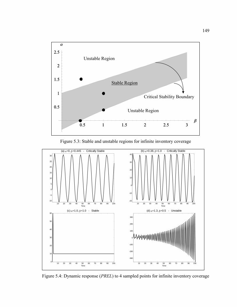
149

0.5 1 1.5 2 2.5 3b

0.5

1

1.5

2

2.5

a

0.5 1 1.5 2 2.5 3b

0.5

1

1.5

2

2.5

a

Critical Stability Boundary

Stable Region

Unstable Region

Unstable Region

Figure 5.3: Stable and unstable regions for infinite inventory coverage

10 20 30 40 50 60 70 80 90 100-10

-5

0

5

10

15

20

25

30

(a) α=0, β=0.445 - Critically Stable

Time10 20 30 40 50 60 70 80 90 100

-20

-10

0

10

20

30

40

(b) α=0.38, β=1.0 - Critically Stable

Time

10 20 30 40 50 60 70 80 90 1000

10

20

30

40

50

60(c) α=1.0, β=1.0 - Stable

Time 10 20 30 40 50 60 70 80 90 100

-300

-200

-100

0

100

200

300

(d) α=1.3, β=0.5 - Unstable

Time

Figure 5.4: Dynamic response (PREL) to 4 sampled points for infinite inventory coverage

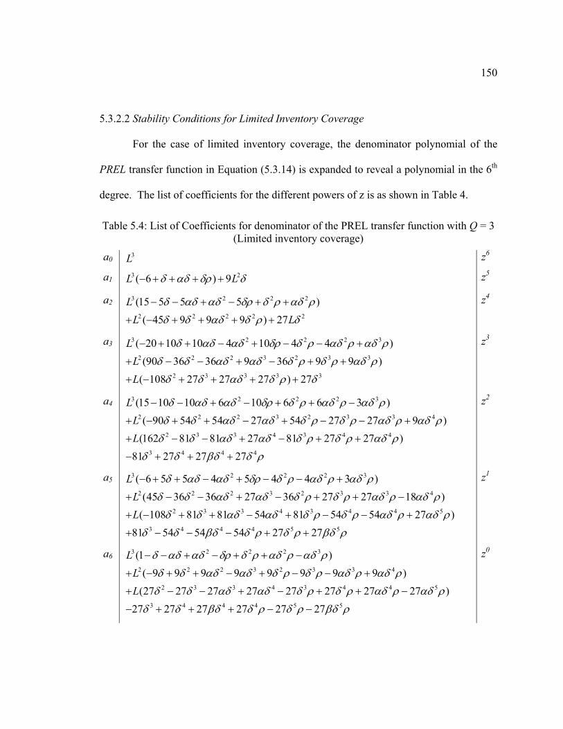
150

5.3.2.2 Stability Conditions for Limited Inventory Coverage

For the case of limited inventory coverage, the denominator polynomial of the

PREL transfer function in Equation (5.3.14) is expanded to reveal a polynomial in the 6th

degree. The list of coefficients for the different powers of z is as shown in Table 4.

Table 5.4: List of Coefficients for denominator of the PREL transfer function with Q = 3 (Limited inventory coverage)

a0 3L z6

a1 3 2( 6 ) 9L Lδ αδ δρ δ− + + + + z5

a2 3 2 2

2 2 2 2

(15 5 5 5 )( 45 9 9 9 ) 27

LL L

2

2

δ αδ αδ δρ δ ρ αδ ρ

δ δ αδ δ ρ δ

− − + − + +

+ − + + + +

z4

a3 3 2 2

2 2 2 3 2 3 3

2 3 3 3 3

( 20 10 10 4 10 4 4 )(90 36 36 9 36 9 9 )

( 108 27 27 27 ) 27

LLL

2 3δ αδ αδ δρ δ ρ αδ ρ αδ ρ

δ δ αδ αδ δ ρ δ ρ αδ ρ

δ δ αδ δ ρ δ

− + + − + − − +

+ − − + − + +

+ − + + + +

z3

a4 3 2 2 2 3

2 2 2 3 2 3 3

2 3 3 4 3 4 4

3 4 4 4

(15 10 10 6 10 6 6 3 )( 90 54 54 27 54 27 27 9 )

(162 81 81 27 81 27 27 )81 27 27 27

LLL

δ αδ αδ δρ δ ρ αδ ρ αδ ρ4δ δ αδ αδ δ ρ δ ρ αδ ρ αδ

δ δ αδ αδ δ ρ δ ρ αδ ρ

δ δ βδ δ ρ

− − + − + + −

+ − + + − + − − +

+ − − + − + +

− + + +

ρ

z2

a5 3 2 2 2 3

2 2 2 3 2 3 3 4

2 3 3 4 3 4 4 5

3 4 4 4 5 5

( 6 5 5 4 5 4 4 3 )(45 36 36 27 36 27 27 18 )

( 108 81 81 54 81 54 54 27 )81 54 54 54 27 27

LLL

δ αδ αδ δρ δ ρ αδ ρ αδ ρ

δ δ αδ αδ δ ρ δ ρ αδ ρ αδ ρ

δ δ αδ αδ δ ρ δ ρ αδ ρ αδ

δ δ βδ δ ρ δ ρ βδ ρ

− + + − + − − +

+ − − + − + + −

+ − + + − + − − +

+ − − − + +

ρ

z1

a6 3 2 2 2 3

2 2 2 3 2 3 3 4

2 3 3 4 3 4 4 5

3 4 4 4 5 5

(1 )( 9 9 9 9 9 9 9 9 )

(27 27 27 27 27 27 27 2727 27 27 27 27 27

LLL

δ αδ αδ δρ δ ρ αδ ρ αδ ρ

δ δ αδ αδ δ ρ δ ρ αδ ρ αδ ρ

)δ δ αδ αδ δ ρ δ ρ αδ ρ αδ

δ δ βδ δ ρ δ ρ βδ ρ

− − + − + + −

+ − + + − + − − +

+ − − + − + + −

− + + + − −

ρ

z0

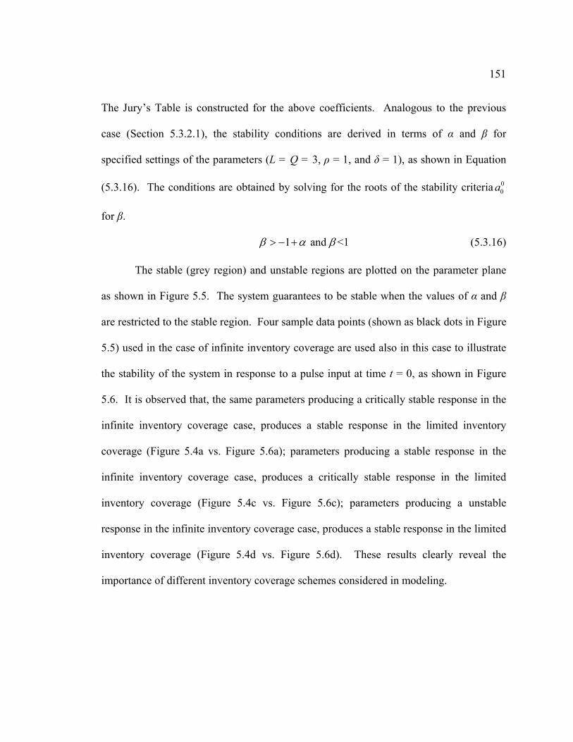
151

The Jury’s Table is constructed for the above coefficients. Analogous to the previous

case (Section 5.3.2.1), the stability conditions are derived in terms of α and β for

specified settings of the parameters (L = Q = 3, ρ = 1, and δ = 1), as shown in Equation

(5.3.16). The conditions are obtained by solving for the roots of the stability criteria

for β.

00a

1 and <1 β α β> − + (5.3.16)

The stable (grey region) and unstable regions are plotted on the parameter plane

as shown in Figure 5.5. The system guarantees to be stable when the values of α and β

are restricted to the stable region. Four sample data points (shown as black dots in Figure

5.5) used in the case of infinite inventory coverage are used also in this case to illustrate

the stability of the system in response to a pulse input at time t = 0, as shown in Figure

5.6. It is observed that, the same parameters producing a critically stable response in the

infinite inventory coverage case, produces a stable response in the limited inventory

coverage (Figure 5.4a vs. Figure 5.6a); parameters producing a stable response in the

infinite inventory coverage case, produces a critically stable response in the limited

inventory coverage (Figure 5.4c vs. Figure 5.6c); parameters producing a unstable

response in the infinite inventory coverage case, produces a stable response in the limited

inventory coverage (Figure 5.4d vs. Figure 5.6d). These results clearly reveal the

importance of different inventory coverage schemes considered in modeling.

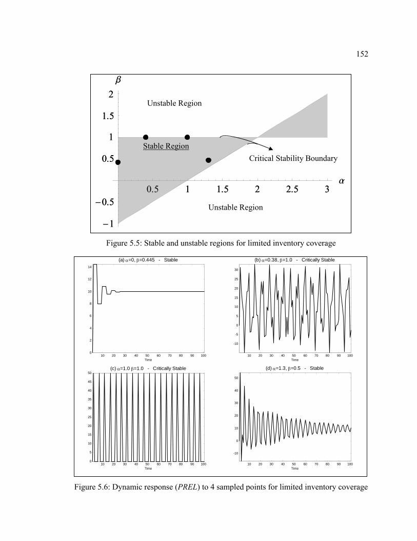
152

0.5 1 1.5 2 2.5 3a

-1

-0.5

0.5

1

1.5

2b

0.5 1 1.5 2 2.5 3a

-1

-0.5

0.5

1

1.5

2b

Critical Stability BoundaryStable Region

Unstable Region

Unstable Region

Figure 5.5: Stable and unstable regions for limited inventory coverage

10 20 30 40 50 60 70 80 90 1000

2

4

6

8

10

12

14

(a) α=0, β=0.445 - Stable

Time 10 20 30 40 50 60 70 80 90 100

-10

-5

0

5

10

15

20

25

30

(b) α=0.38, β=1.0 - Critically Stable

Time

10 20 30 40 50 60 70 80 90 1000

5

10

15

20

25

30

35

40

45

50(c) α=1.0 β=1.0 - Critically Stable

Time 10 20 30 40 50 60 70 80 90 100

-10

0

10

20

30

40

50

(d) α=1.3, β=0.5 - Stable

Time

Figure 5.6: Dynamic response (PREL) to 4 sampled points for limited inventory coverage

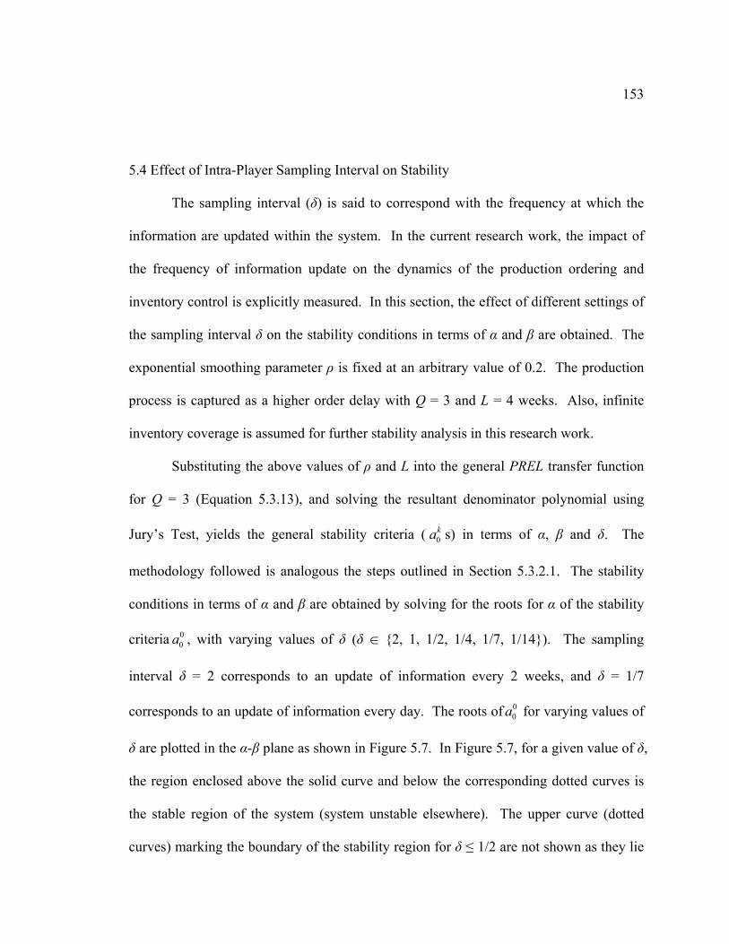
153

5.4 Effect of Intra-Player Sampling Interval on Stability


information are updated within the system. In the current research work, the impact of

the frequency of information update on the dynamics of the production ordering and

inventory control is explicitly measured. In this section, the effect of different settings of

the sampling interval δ on the stability conditions in terms of α and β are obtained. The

exponential smoothing parameter ρ is fixed at an arbitrary value of 0.2. The production

process is captured as a higher order delay with Q = 3 and L = 4 weeks. Also, infinite

inventory coverage is assumed for further stability analysis in this research work.

Substituting the above values of ρ and L into the general PREL transfer function

for Q = 3 (Equation 5.3.13), and solving the resultant denominator polynomial using

Jury’s Test, yields the general stability criteria ( s) in terms of α, β and δ. The

methodology followed is analogous the steps outlined in Section 5.3.2.1. The stability

conditions in terms of α and β are obtained by solving for the roots for α of the stability

criteria , with varying values of δ (δ œ {2, 1, 1/2, 1/4, 1/7, 1/14}). The sampling

interval δ = 2 corresponds to an update of information every 2 weeks, and δ = 1/7

corresponds to an update of information every day. The roots of for varying values of

δ are plotted in the α-β plane as shown in Figure 5.7. In Figure 5.7, for a given value of δ,

the region enclosed above the solid curve and below the corresponding dotted curves is

the stable region of the system (system unstable elsewhere). The upper curve (dotted

curves) marking the boundary of the stability region for δ ≤ 1/2 are not shown as they lie

0ka

00a

00a

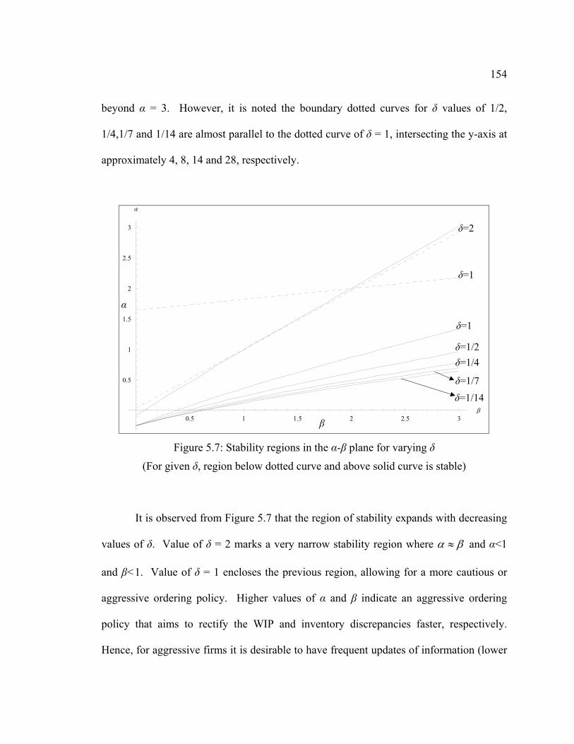
154

beyond α = 3. However, it is noted the boundary dotted curves for δ values of 1/2,

1/4,1/7 and 1/14 are almost parallel to the dotted curve of δ = 1, intersecting the y-axis at

approximately 4, 8, 14 and 28, respectively.

0.5 1 1.5 2 2.5 3b

0.5

1

1.5

2

2.5

3

a

δ=1

δ=1

δ=1/2δ=1/4

δ=1/7

δ=1/14

δ=2

β

α

Figure 5.7: Stability regions in the α-β plane for varying δ

(For given δ, region below dotted curve and above solid curve is stable)

It is observed from Figure 5.7 that the region of stability expands with decreasing

values of δ. Value of δ = 2 marks a very narrow stability region where α β≈ and α<1

and β<1. Value of δ = 1 encloses the previous region, allowing for a more cautious or

aggressive ordering policy. Higher values of α and β indicate an aggressive ordering

policy that aims to rectify the WIP and inventory discrepancies faster, respectively.

Hence, for aggressive firms it is desirable to have frequent updates of information (lower

155

δ), to ensure that system performs within the stable region. Also, it is clear that firms

ordering only based on the end inventory levels ignoring the current WIP or supply line

(α = 0, β>0) becomes unstable even if it fully accounts for the inventory levels (β = 1),

allowing only for very cautious ordering policy ( 0.5β ≺ ). This condition remains true

even for very frequent updates of information.

5.4.1 Investigation of a Special Case: α = β

The setting of α = β, which is referred to as the Deziel-Eilon arbitrary setting

(1967), results in the production release order rate to be stable for all values of α = β

(Towill 1980, Disney and Towill 2002). Specifically, the transfer function of production

release rate is found to be stable for a pipeline delayed production process with sampling

interval of δ=1. It is of our interest to understand the effect of varied sampling intervals

on the stability when α = β.

Setting α = β reduces the PREL transfer function (with Q = 3) in Equation

(5.3.13) to the Equation (5.4.1) shown below:

[ ] (( 1) ( 1 ( 1 ) (1 )))[ ] ( 1 )( 1 )

MiMi

PREL z z L zSALES z z z

Lδ ρ α δ ρ ρ ρδρ αδ

− + − + − − + + + +=

− + + − + + (5.4.1)

Given the simplistic nature of the transfer function, the poles and zeros can be directly

computed without resort to the Jury’s Test, as shown in Table 5.5. Upon inspection of

the poles, it is immediately apparent that the system is always stable if ( ) 2α βδ

= <

(poles must lie within the unit circle in the complex plane for stability). This relation is

critical in selecting the appropriate (though equal) values of α = β based on the frequency

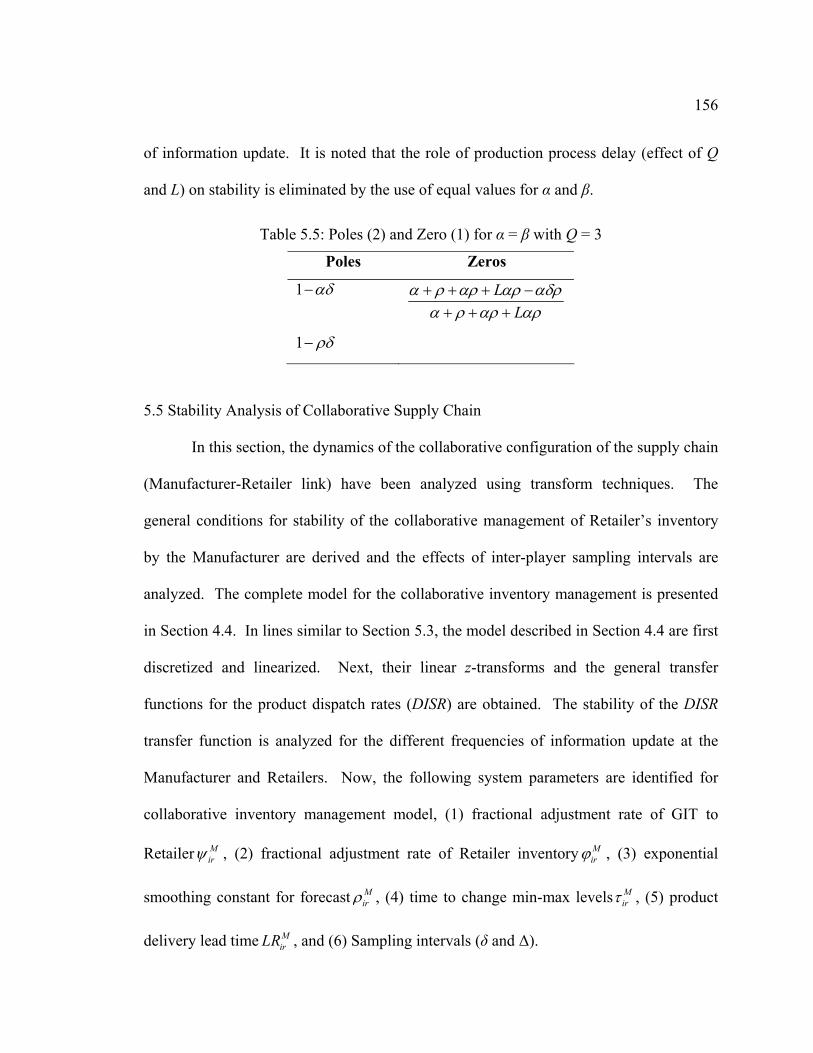
156

of information update. It is noted that the role of production process delay (effect of Q

and L) on stability is eliminated by the use of equal values for α and β.

Table 5.5: Poles (2) and Zero (1) for α = β with Q = 3

Poles Zeros

1 αδ− LL

α ρ αρ αρ αδρα ρ αρ αρ+ + + −

+ + +

1 ρδ−

5.5 Stability Analysis of Collaborative Supply Chain

In this section, the dynamics of the collaborative configuration of the supply chain

(Manufacturer-Retailer link) have been analyzed using transform techniques. The

general conditions for stability of the collaborative management of Retailer’s inventory

by the Manufacturer are derived and the effects of inter-player sampling intervals are

analyzed. The complete model for the collaborative inventory management is presented

in Section 4.4. In lines similar to Section 5.3, the model described in Section 4.4 are first

discretized and linearized. Next, their linear z-transforms and the general transfer

functions for the product dispatch rates (DISR) are obtained. The stability of the DISR

transfer function is analyzed for the different frequencies of information update at the

Manufacturer and Retailers. Now, the following system parameters are identified for

collaborative inventory management model, (1) fractional adjustment rate of GIT to

Retailer Mirψ , (2) fractional adjustment rate of Retailer inventory M

irϕ , (3) exponential

smoothing constant for forecast Mirρ , (4) time to change min-max levels M

irτ , (5) product

delivery lead time MirLR , and (6) Sampling intervals (δ and ∆).

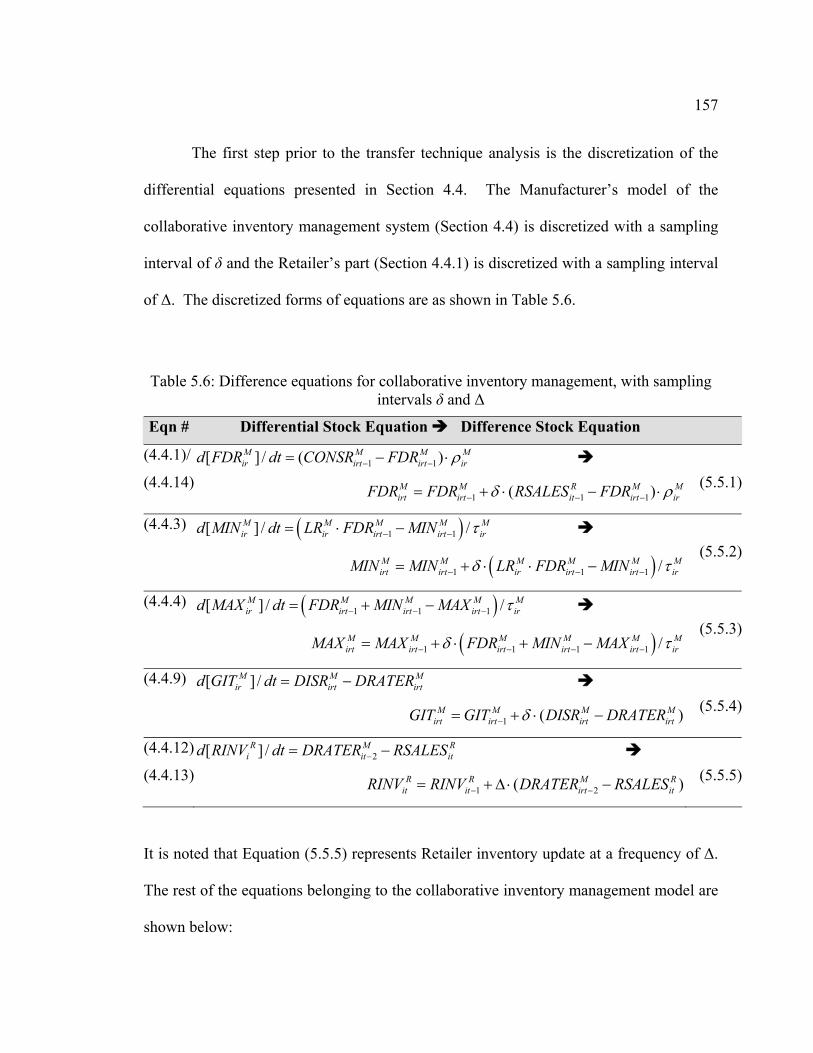
157

The first step prior to the transfer technique analysis is the discretization of the

differential equations presented in Section 4.4. The Manufacturer’s model of the

collaborative inventory management system (Section 4.4) is discretized with a sampling

interval of δ and the Retailer’s part (Section 4.4.1) is discretized with a sampling interval

of ∆. The discretized forms of equations are as shown in Table 5.6.

Table 5.6: Difference equations for collaborative inventory management, with sampling intervals δ and ∆


(4.4.1)/

(4.4.14)1 1[ ] / ( )M M M M

ir irt irt irFDR dt CONSR FDRd ρ− −= − ⋅

1

1 1( )M M R Mirt irt it irt irFDR FDR RSALES FDR Mδ ρ− − −= + ⋅ − ⋅ (5.5.1)

(4.4.3) ( )1 1[ ] / /M M M Mir ir irt irt ird MIN dt LR FDR MIN Mτ− −= ⋅ −

( )1 1 /1M M M M Mirt irt ir irt irt irMIN MIN LR FDR MIN Mδ τ− −= + ⋅ ⋅ − −

(5.5.2)

(4.4.4) ( )1 1 1[ ] / /M M M Mir irt irt irt ird MAX dt FDR MIN MAX Mτ− − −= + −

( )1 1 1 1 /M M M M Mirt irt irt irt irt irMAX MAX FDR MIN MAX Mδ τ− − − −= + ⋅ + −

(5.5.3)

(4.4.9) [ ] /M Mir irt irtd GIT dt DISR DRATER= − M

M

1 ( )M M Mirt irt irt irtGIT GIT DISR DRATERδ−= + ⋅ − (5.5.4)

(4.4.12)

(4.4.13)2[ ] /R M

i itd RINV dt DRATER RSALES−= − Rit

R

1 2( )R R Mit it irt itRINV RINV DRATER RSALES− −= + ∆ ⋅ − (5.5.5)

It is noted that Equation (5.5.5) represents Retailer inventory update at a frequency of ∆.

The rest of the equations belonging to the collaborative inventory management model are

shown below:

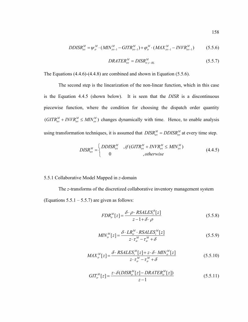
158

1 1 1( ) (M M M M M M Mirt ir irt irt ir irt irtDDISR MIN GITR MAX INVRψ ϕ 1)− − −= ⋅ − + ⋅ − −

)M

(5.5.6)

(5.5.7) ,M Mirt ir t RLDRATER DISR −=

The Equations (4.4.6)-(4.4.8) are combined and shown in Equation (5.5.6).

The second step is the linearization of the non-linear function, which in this case

is the Equation 4.4.5 (shown below). It is seen that the DISR is a discontinuous

piecewise function, where the condition for choosing the dispatch order quantity

changes dynamically with time. Hence, to enable analysis

using transformation techniques, it is assumed that

( M Mirt irt irtGITR INVR MIN+ ≤

M Mirt irtDISR DDISR= at every time step.

(4.4.5) , ( )

0 ,



otherwise⎧ + ≤

= ⎨⎩

M

5.5.1 Collaborative Model Mapped in z-domain

The z-transforms of the discretized collaborative inventory management system

(Equations 5.5.1 – 5.5.7) are given as follows:

[ ][ ]1

RM iir

RSALES zFDR zz

δ ρδ ρ

⋅ ⋅=

− + ⋅ (5.5.8)

[ ][ ]M M

M ir iir M M

ir ir

LR RSALES zMIN zz

δτ τ δ

⋅ ⋅=

⋅ − + (5.5.9)

[ ] [ ][ ]M M

M iir M M

ir ir

irRSALES z z MIN zMAX zz

δ δτ τ δ

⋅ + ⋅ ⋅=

⋅ − + (5.5.10)

( [ ] [[ ]1

M MM ir ir

irz DISR z DRATER zGIT z

zδ⋅ −

=−

]) (5.5.11)

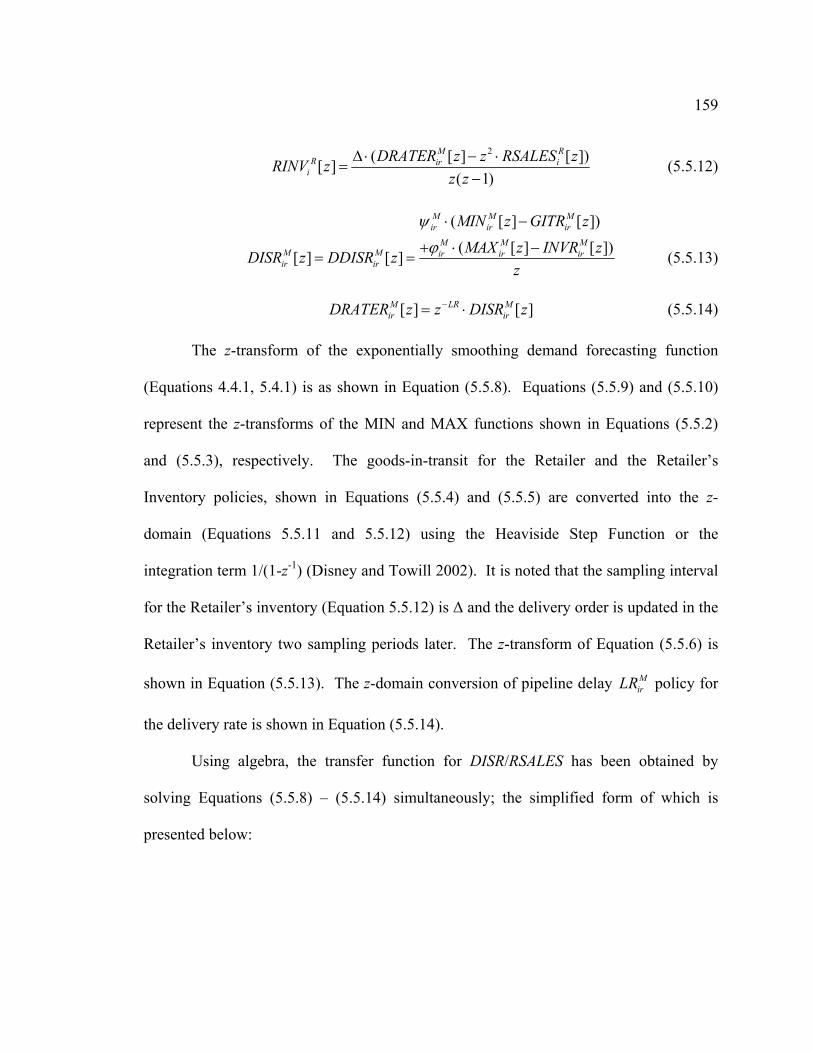
159

2( [ ][ ]

( 1)

M RR ir i

iDRATER z z RSALES zRINV z

z z∆ ⋅ − ⋅

=−

[ ]) (5.5.12)

( [ ] [ ])

( [ ] [[ ] [ ]

M M Mir ir ir

M M MM M ir ir irir ir

MIN z GITR z

])MAX z INVR zDISR z DDISR zz

ψ

ϕ

⋅ −

+ ⋅ −= = (5.5.13)

(5.5.14) [ ] [ ]M LR Mir irDRATER z z DISR z−= ⋅

The z-transform of the exponentially smoothing demand forecasting function

(Equations 4.4.1, 5.4.1) is as shown in Equation (5.5.8). Equations (5.5.9) and (5.5.10)

represent the z-transforms of the MIN and MAX functions shown in Equations (5.5.2)

and (5.5.3), respectively. The goods-in-transit for the Retailer and the Retailer’s

Inventory policies, shown in Equations (5.5.4) and (5.5.5) are converted into the z-

domain (Equations 5.5.11 and 5.5.12) using the Heaviside Step Function or the

integration term 1/(1-z-1) (Disney and Towill 2002). It is noted that the sampling interval

for the Retailer’s inventory (Equation 5.5.12) is ∆ and the delivery order is updated in the

Retailer’s inventory two sampling periods later. The z-transform of Equation (5.5.6) is

shown in Equation (5.5.13). The z-domain conversion of pipeline delay MirLR policy for

the delivery rate is shown in Equation (5.5.14).

Using algebra, the transfer function for DISR/RSALES has been obtained by

solving Equations (5.5.8) – (5.5.14) simultaneously; the simplified form of which is

presented below:

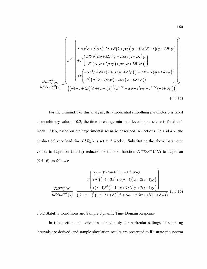
160

( )( ) ( )( )( )

( ) ( )( )( ) ( )( )

( ) ( )( )

4 2 3 2

3 21 2

2

2 3

2

3 2

3 2 2

2

2 1

2 2[ ][ ]

LR

Mir

Ri

z z LR

LRz z

LR

LR LRz

LRDISR zRSALES z

τ ϕ τ τ δ ρτ ϕ δ ρ δ τ ϕ ψ

δ ρϕ τ ϕ δ τ ρτ ϕ

δ ϕ ρτϕ ρτ ϕ ψ

τ ϕ δ τ ρτ ϕ δ ρ ϕ ψ

δ ϕ ρτϕ ρτ ϕ ψ

+

⎛ ⎛ ⎞⎜ ⎟⎜ ⎟∆ + ∆ − + + − − + ⋅⎜ ⎟⎜ ⎟⎛ ⎞⋅ + ∆ − ∆ +⎜ ⎟⎜ ⎟+

⎜ ⎟⎜ ⎟+ ∆ + + + ⋅⎝ ⎠⎜ ⎟⎜ ⎟⎛ ⎞−∆ + ∆ + + − + ∆ + ⋅⎜ ⎟⎜ ⎟+

⎜ ⎟⎜ ⎟− ∆ + + + ⋅⎝ ⎠⎝ ⎠⎝=( ) ( )( ) ( )( )( )2 3 2 21 1 1LR LRz z z z zδρ δ τ ϕ δψ δψ+ +

⎞⎜ ⎟⎜ ⎟⎜ ⎟⎜ ⎟⎜ ⎟⎜ ⎟⎜ ⎟⎜ ⎟⎜ ⎟⎜ ⎟

⎠

− + + + − + ∆ − + − +

(5.5.15)

For the remainder of this analysis, the exponential smoothing parameter ρ is fixed

at an arbitrary value of 0.2; the time to change min-max levels parameter τ is fixed at 1

week. Also, based on the experimental scenario described in Sections 3.5 and 4.7, the

product delivery lead time ( MirLR ) is set at 2 weeks. Substituting the above parameter

values to Equation (5.5.15) reduces the transfer function DISR/RSALES to Equation

(5.5.16), as follows:

( )( )( )( )

( ) ( )( )

3 2

3 3 2

2

2 5 2 4

5( 1) 11( 1)

1 2 ( 1) 2( 1)

( 1) 1 7 2( 1)[ ][ ] 1 5 5 ( 1 )

Mir

Ri

z z z z

z z z z

z z z zDISR zRSALES z z z z z z

ϕ δ ϕ

δ ϕ

δ ϕ ψ

ψ

δ δ ϕ δψ δψ

⎛ ⎞− ∆ + − ∆⎜ ⎟⎜ ⎟+ − + + ∆ − + −⎜ ⎟⎜ ⎟+ − − + + ∆ + −⎝ ⎠=

+ − − + + + ∆ − + − + (5.5.16)

5.5.2 Stability Conditions and Sample Dynamic Time Domain Response

In this section, the conditions for stability for particular settings of sampling

intervals are derived, and sample simulation results are presented to illustrate the system

161

response. The sampling intervals ∆ and δ are set equal to 1 week. Substituting the values

of ∆ and δ into Equation (5.4.16),

( )( )

( )( )2 2 3

5 2 4

3 3 4 5 2( 1)[ ][ ] 4 5 ( 1 )

Mir

Ri

z z z z zDISR zRSALES z z z z z

ϕ ψ

ϕ ψ ψ

− + − + + −=

− + + − + − + (5.5.17)

The denominator polynomial of the DISR transfer function in Equation (5.5.17) is

expanded to reveal a polynomial in the 6th degree. The coefficients of z are used to

construct the Jury’s Table (not shown). For stability, all s (with k = 1…5) must be

positive. In the Jury table, the s in their natural form are very lengthy mathematical

expressions, which are not shown in this paper for the sake of brevity. Now, the stability

conditions are derived in terms of ψ and φ by solving for the roots of .

0

ka

0

ka

0

0a

The stability conditions are illustrated on the ψ-φ parameter plane, as shown in

Figure 5.8. Each curve in Figure 5.8 illustrates a stability condition. The stable region is

below the dotted lines and above the solid line, to the left of the intersection of the curves.

The system is guaranteed to be stable when the values of ψ and φ are restricted to the

stable region.

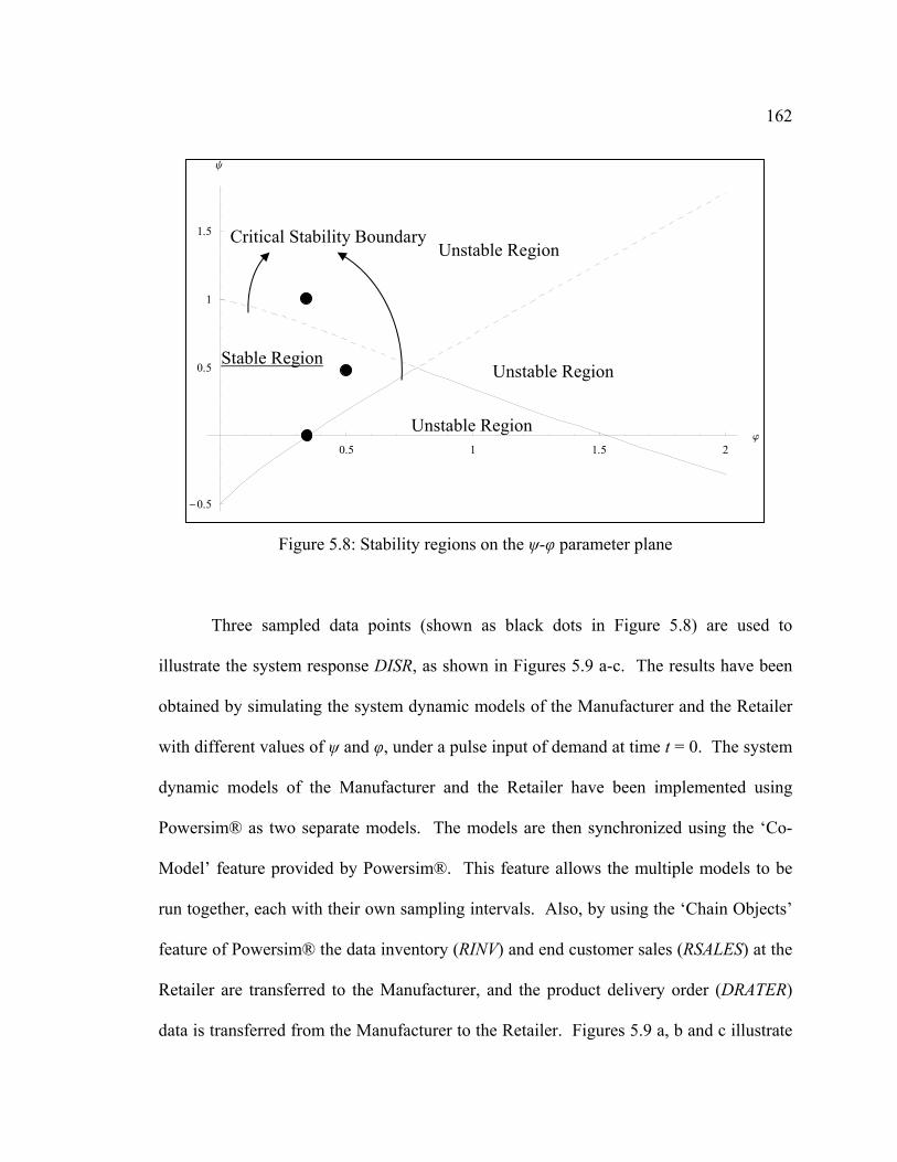
162

0.5 1 1.5 2j

-0.5

0.5

1

1.5

y

Critical Stability Boundary

Stable Region

Unstable Region

Unstable Region

Unstable Region

Figure 5.8: Stability regions on the ψ-φ parameter plane

Three sampled data points (shown as black dots in Figure 5.8) are used to

illustrate the system response DISR, as shown in Figures 5.9 a-c. The results have been

obtained by simulating the system dynamic models of the Manufacturer and the Retailer

with different values of ψ and φ, under a pulse input of demand at time t = 0. The system

dynamic models of the Manufacturer and the Retailer have been implemented using

Powersim® as two separate models. The models are then synchronized using the ‘Co-

Model’ feature provided by Powersim®. This feature allows the multiple models to be

run together, each with their own sampling intervals. Also, by using the ‘Chain Objects’

feature of Powersim® the data inventory (RINV) and end customer sales (RSALES) at the

Retailer are transferred to the Manufacturer, and the product delivery order (DRATER)

data is transferred from the Manufacturer to the Retailer. Figures 5.9 a, b and c illustrate

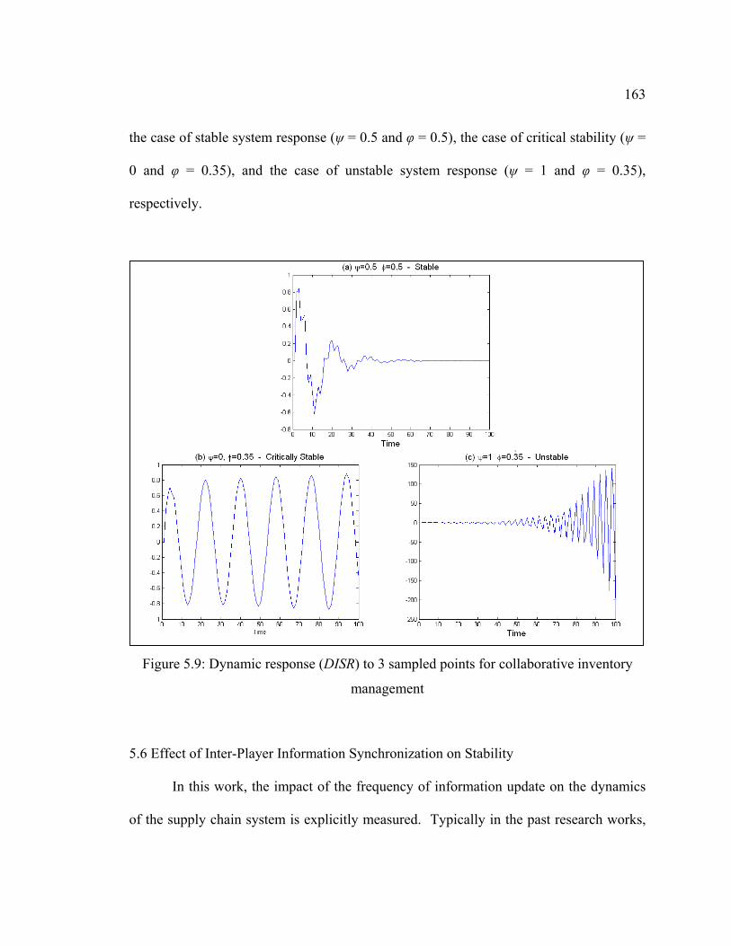
163

the case of stable system response (ψ = 0.5 and φ = 0.5), the case of critical stability (ψ =

0 and φ = 0.35), and the case of unstable system response (ψ = 1 and φ = 0.35),

respectively.

Figure 5.9: Dynamic response (DISR) to 3 sampled points for collaborative inventory

management

5.6 Effect of Inter-Player Information Synchronization on Stability

In this work, the impact of the frequency of information update on the dynamics

of the supply chain system is explicitly measured. Typically in the past research works,

164

the frequency at which the Retailer sends their demand and inventory information to the

Manufacturer is the same as the frequency at which the Manufacturer makes decisions

(e.g. Disney and Towill 2002). That is, if the frequency or sampling interval for making

decisions at the Manufacturer is every week then the Retailer sends updated data every

week. In this section, the possible differences in the frequency of information update at

the different players and their effect on overall system stability are analyzed. That is,

what happens when the Manufacturer updates its information every day but the Retailers

send their updated information every week? How should the decision parameters at the

Manufacturer be selected so that system operation accounts for the difference in the

update frequency and continues to be stable?


information are updated within the Manufacturer. The sampling interval (∆) is said to

correspond with the frequency at which the information are updated within the Retailer

(hence the frequency at which updated data is sent from Retailer to Manufacturer). The

effect of different settings of the sampling intervals δ and ∆ on the stability conditions in

terms of ψ and φ are analyzed in the following sub-sections.

5.6.1 Case I: δ = ∆

First, the effect of setting the sampling intervals such that the ratio ∆/ δ = 1 is

analyzed. That is, frequency at which the Retailer sends their demand and inventory

information to the Manufacturer is the same as the frequency at which the Manufacturer

makes decisions. The stability conditions in terms of ψ and φ are obtained (similar to

165

Section 5.5.2) for each of the following cases: δ = ∆ = 1, δ = ∆ = 1/2, δ = ∆ = 1/7. The

sampling interval 1/2 corresponds to an update of information twice a week, and an

interval of 1/7 corresponds to update of information every day.

The stability conditions for the different settings of the sampling interval are

plotted in the ψ – φ parameter plane, as shown in Figure 5.10. In Figure 5.10, curves of

the same color represent the stability conditions for a particular setting of the sampling

interval. For each setting, the stable region is below the dotted lines and above the solid

line, and to the left of the intersection of the curves.

It is observed from Figure 5.10 that, the region of stability for sampling interval

equal to 1 week (black color curves) is enclosed by the region of stability for sampling

interval equal to 1/2 (red color curves), which in turn, is enclosed by the region of

stability for sampling interval equal to 1/7 (blue color curves). Now, higher values of ψ

and φ indicate an aggressive ordering policy that aims to rectify the inventory and good-

in-transit discrepancies faster. The sampling interval settings of 1/7 (daily updates)

presents the largest stability region, thus allowing for a more aggressive ordering policy.

Consequently, the sampling interval settings of 1 (weekly updates) allows for a very

cautious ordering policy. This ascertains a partly intuitive result that for aggressive firms

it is desirable to have frequent updates of information albeit other factors such as the

costs of information are trivial.

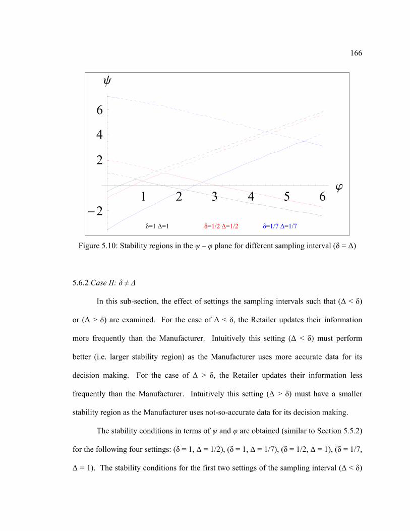
166

1 2 3 4 5 6j

-2

2

4

6

y

δ=1 ∆=1 δ=1/2 ∆=1/2 δ=1/7 ∆=1/7

Figure 5.10: Stability regions in the ψ – φ plane for different sampling interval (δ = ∆)

5.6.2 Case II: δ ≠ ∆

In this sub-section, the effect of settings the sampling intervals such that (∆ < δ)

or (∆ > δ) are examined. For the case of ∆ < δ, the Retailer updates their information

more frequently than the Manufacturer. Intuitively this setting (∆ < δ) must perform

better (i.e. larger stability region) as the Manufacturer uses more accurate data for its

decision making. For the case of ∆ > δ, the Retailer updates their information less

frequently than the Manufacturer. Intuitively this setting (∆ > δ) must have a smaller

stability region as the Manufacturer uses not-so-accurate data for its decision making.

The stability conditions in terms of ψ and φ are obtained (similar to Section 5.5.2)

for the following four settings: (δ = 1, ∆ = 1/2), (δ = 1, ∆ = 1/7), (δ = 1/2, ∆ = 1), (δ = 1/7,

∆ = 1). The stability conditions for the first two settings of the sampling interval (∆ < δ)

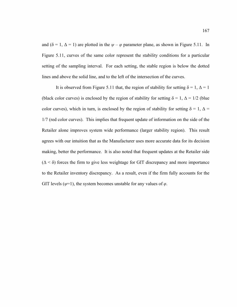
167

and (δ = 1, ∆ = 1) are plotted in the ψ – φ parameter plane, as shown in Figure 5.11. In

Figure 5.11, curves of the same color represent the stability conditions for a particular

setting of the sampling interval. For each setting, the stable region is below the dotted

lines and above the solid line, and to the left of the intersection of the curves.

It is observed from Figure 5.11 that, the region of stability for setting δ = 1, ∆ = 1

(black color curves) is enclosed by the region of stability for setting δ = 1, ∆ = 1/2 (blue

color curves), which in turn, is enclosed by the region of stability for setting δ = 1, ∆ =

1/7 (red color curves). This implies that frequent update of information on the side of the

Retailer alone improves system wide performance (larger stability region). This result

agrees with our intuition that as the Manufacturer uses more accurate data for its decision

making, better the performance. It is also noted that frequent updates at the Retailer side

(∆ < δ) forces the firm to give less weightage for GIT discrepancy and more importance

to the Retailer inventory discrepancy. As a result, even if the firm fully accounts for the

GIT levels (ψ=1), the system becomes unstable for any values of φ.

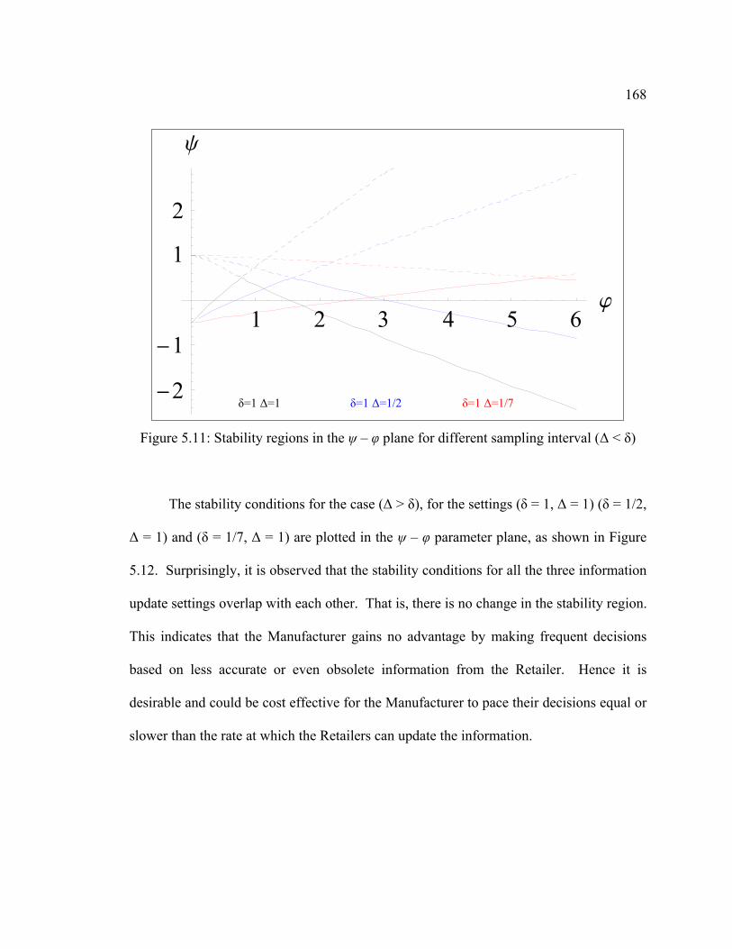
168

1 2 3 4 5 6j

-2

-1

1

2

y

δ=1 ∆=1/2 δ=1 ∆=1 δ=1 ∆=1/7

Figure 5.11: Stability regions in the ψ – φ plane for different sampling interval (∆ < δ)

The stability conditions for the case (∆ > δ), for the settings (δ = 1, ∆ = 1) (δ = 1/2,

∆ = 1) and (δ = 1/7, ∆ = 1) are plotted in the ψ – φ parameter plane, as shown in Figure

5.12. Surprisingly, it is observed that the stability conditions for all the three information

update settings overlap with each other. That is, there is no change in the stability region.

This indicates that the Manufacturer gains no advantage by making frequent decisions

based on less accurate or even obsolete information from the Retailer. Hence it is

desirable and could be cost effective for the Manufacturer to pace their decisions equal or

slower than the rate at which the Retailers can update the information.

169

1 2 3 4 5 6j

-2

2

4

6y

δ=1/2 ∆=1 δ=1 ∆=1 δ=1/7 ∆=1

Figure 5.12: Stability regions in the ψ – φ plane for different sampling interval (∆ > δ)

5.7 Conditions for Stability for Each Player in the Supply Chain Scenario

In this section, the stability conditions for each player of the supply chain are

obtained. These conditions are suited to the supply chain scenario described in Section

3.5 and the parameters presented in Section 4.7. The Manufacturer’s product production

management (see Section 4.3.1), Manufacturer’s component ordering (see Section 4.3.2),

and Supplier’s component production management (see Section 4.5.1) can be directly

mapped to the general production-inventory control system described (see Section 5.3).

Hence their stability conditions are obtained from the transfer function for the general

production-inventory control system presented in Sections 5.3.1.1 and 5.3.1.2. Also, the

stability conditions for the collaborative management of Retailer’s inventory model are

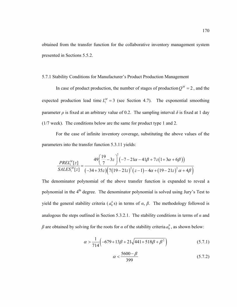
170

obtained from the transfer function for the collaborative inventory management system

presented in Sections 5.5.2.

5.7.1 Stability Conditions for Manufacturer’s Product Production Management

In case of product production, the number of stages of production , and the

expected production lead time

2MQ =

3MiL = (see Section 4.7). The exponential smoothing

parameter ρ is fixed at an arbitrary value of 0.2. The sampling interval δ is fixed at 1 day

(1/7 week). The conditions below are the same for product type 1 and 2.

For the case of infinite inventory coverage, substituting the above values of the

parameters into the transfer function 5.3.11 yields:

( )( )

( ) ( ) ( ) ( )( )

2

2

1949 3 7 21 41 7 1 3 6[ ] 7[ ] 34 35 7 19 21 1 4 19 21 4

MiMi

z zPREL z

SALES z z z z z

α β α β

2α α β

⎛ ⎞− − − − + + +⎜ ⎟⎝ ⎠=

− + − − − + − +

The denominator polynomial of the above transfer function is expanded to reveal a

polynomial in the 4th degree. The denominator polynomial is solved using Jury’s Test to

yield the general stability criteria ( s) in terms of α, β. The methodology followed is

analogous the steps outlined in Section 5.3.2.1. The stability conditions in terms of α and

β are obtained by solving for the roots for α of the stability criteria , as shown below:

0ka

00a

( )21 679 13 21 441 518714

α β β> − + + + + β (5.7.1)

5600399

βα −< (5.7.2)

171

For the case of limited inventory coverage, substituting the above values of the

parameters into the transfer function 5.3.12 yields:

2

3

2

[ ] (19 21 ) (7 6)(1 3 )[ ] 2166 3087 (7315 735 )

( 34 35 )306 147 ( 56 3 ) 4

MiMi

PREL z z zSALES z z z

zz

α βα

α α

− − + +=

⎛ ⎞− + + −− + ⎜ ⎟⎜ ⎟+ + − + +⎝ ⎠β

The denominator polynomial is solved using Jury’s Test to yield the general stability

conditions in terms of α, β:

( )21 13371 76 49 441 12408 169180

α β β> − + + + + β (5.7.3)

2(5200 )741

βα −< (5.7.4)

5.7.2 Stability Conditions for Manufacturer’s Component Ordering

Component ordering is a special case of the general production-inventory control

system with pipeline material delay and no demand forecasting. Pipeline delay is

modeled using the general production-inventory control system by setting by setting

MjQ CL= where the component supplies delay 2M

jCL = (see Section 4.7). To model no

forecasting, the exponential smoothing parameter ρ is set at 1. The sampling interval δ is

fixed at 1 day (1/7 week). Also, the terms γ and η are used instead of α and β respectively,

to make it consistent with the description of the model in Section 4.3.2. The conditions

below are the same for component type 1 and 2.


parameters into the transfer function 5.3.11 yields,

172

( ) ( )( )

( ) ( )3 2

6 7 7 14 13 7 1 2 2[ ][ ] 252 343 49 19 84 10 35

MjMj

z zCORD zDUSG z z z z

γ η λ ηγ γ γ

− + − − − + + +=− + + − − − + +η



yield the general stability criteria ( s) in terms of γ, η. The methodology followed is

analogous the steps outlined in Section 5.3.2.1. The stability conditions in terms of γ and

η are obtained by solving for the roots for γ of the stability criteria , as shown below:

0ka

00a

( )21 217 3 7 441 322140

γ η η> − + + + +η (5.7.5)

2366168

ηγ −< (5.7.6)



( )2

3 2

[ ] (6 7 ) (1 2 )[ ] 216 343 (756 77 ) 49 ( 18 ) 30

MjMj

CORD z zDUSG z z z z

α βα α α β

− + +=

− + + − + − + + +

The denominator polynomial is solved using Jury’s Test to yield the general stability

conditions in terms of γ, η:

( )21 13371 76 49 441 12408 169180

γ η η> − + + + + η (5.7.7)

2(5200 )741

ηγ −< (5.7.8)

5.7.3 Stability Conditions for Suppliers’ Component Production Management

Among the two suppliers in the system, Supplier 2 is structured similar to the

Manufacturer (see Section 3.5.4). Hence the stability conditions derived for the

173

Manufacturer’s product production management (see Section 4.3.1) is also set as the

stability conditions for Supplier 2.

In the case of Supplier 1 production, the component production delay 11 2SSL ≅

weeks, and the number of production stages 1 1SSQ = (see Section 4.7). The exponential

smoothing parameter ρ is set at 0.2. To analyze the effect of different sampling intervals

for different players on the supply chain, the sampling interval δ of Supplier 1 is fixed at

1 week.



( )( )( ) ( )( )2

[ ] 1 2 1 2 2 5 6[ ] 4 5 1 2 2 3 2

SjSj

SPREL z z z z zSSALES z z z z

α α β βα α β

− + − + − + − +=

− + + − + − + +



yield the general stability criteria ( s) in terms of α, β. The methodology followed is

analogous the steps outlined in Section 5.3.2.1. The stability conditions in terms of α and

β are obtained by solving for the roots for α of the stability criteria , as shown below:

0ka

00a

(1 12

)α β> − + (5.7.9)

64βα +

< (5.7.10)



174

( )( )2

[ ] ( 1 2 )(1 2 )[ ] 4 5 2 ( 1 2 )

SjSj

SPREL z z zSSALES z z z z

α βα β

− + + +=

− + + − + +

The denominator polynomial is solved using Jury’s Test to yield the stability conditions

in terms of α, β:

32βα +

< (5.7.11)

52

β < (5.7.12)

5.7.4 Stability Conditions for Collaborative Inventory Management

In the supply chain scenario considered, there are three Retailers. Hence, the

collaborative inventory management model described in Section 4.4 is repeated for each

Retailer. The sampling interval δ for the Manufacturer is fixed at 1 day (1/7 week). The

expected product transportation lead time 2RiLR = . The exponential smoothing

parameter ρ is fixed at an arbitrary value of 0.2 and the time to change the min-max

levels τ is fixed at an arbitrary value of 1 week for all products and all Retailers. To

analyze the effect of different sampling intervals for different players on the supply chain,

the sampling intervals ∆1 and ∆2 of Retailer1 and Retailer2 respectively, are fixed at 1

day (1/7 week), and the sampling interval ∆3 of Retailer3 is fixed at 1 week. The

conditions below are the same for product type 1 and 2. It is recalled that the Equation

(5.5.16) represents the DISR transfer function in terms of the parameters ψ, φ, δ, and ∆,

with , and2RiLR = 0.2M

irρ = 1Mirτ = .

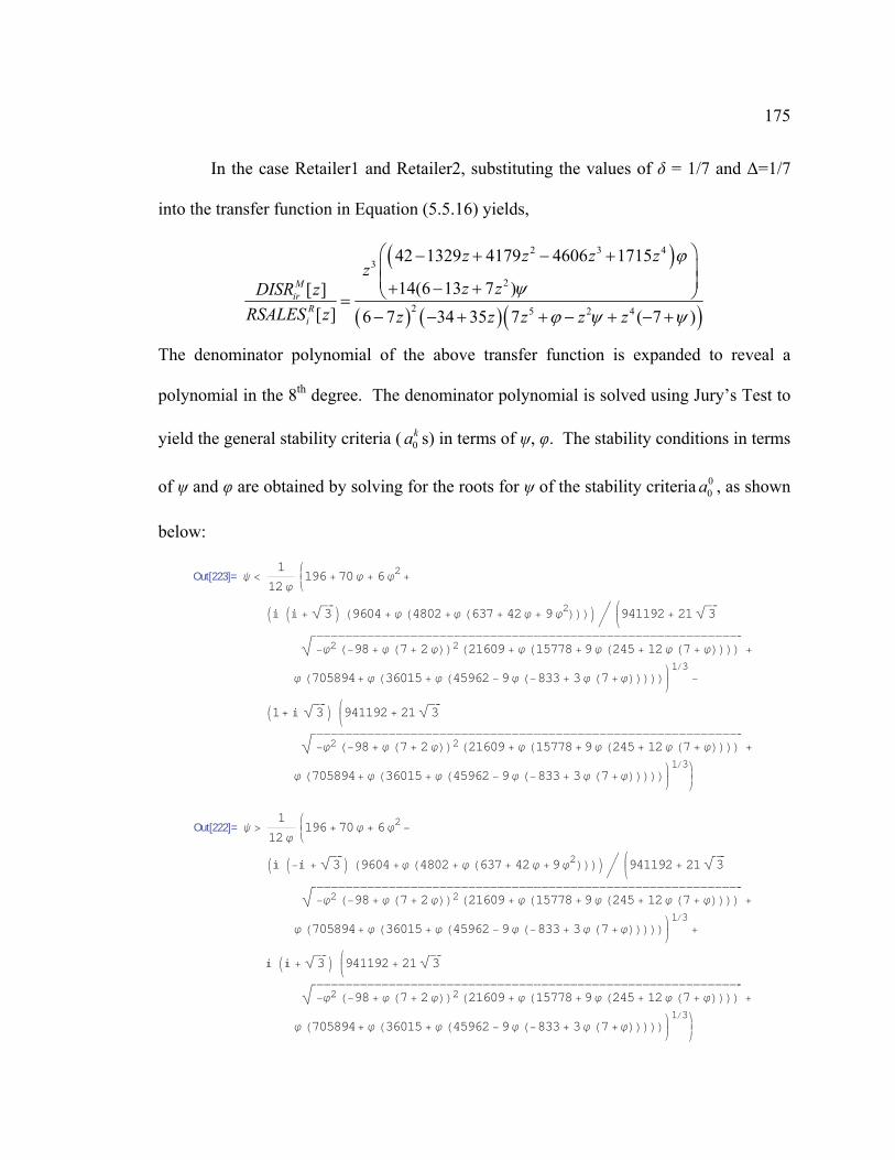
175

In the case Retailer1 and Retailer2, substituting the values of δ = 1/7 and ∆=1/7

into the transfer function in Equation (5.5.16) yields,

( )

( ) ( )( )

2 3 43

2

2 5 2 4

42 1329 4179 4606 1715

14(6 13 7 )[ ][ ] 6 7 34 35 7 ( 7 )

Mir

Ri

z z z zz

z zDISR zRSALES z z z z z z

ϕ

ψ

ϕ ψ ψ

⎛ ⎞− + − +⎜ ⎟⎜ ⎟+ − +⎝ ⎠=− − + + − + − +



yield the general stability criteria ( s) in terms of ψ, φ. The stability conditions in terms

of ψ and φ are obtained by solving for the roots for ψ of the stability criteria , as shown

below:

0ka

00a

Out[223]= ψ <1

12ϕikjj196+70ϕ + 6ϕ2+

I I +è!!!!3M H9604+ ϕ H4802+ϕ H637+ 42ϕ + 9ϕ2LLLM ì i

kjj941192+ 21è!!!!3

"################################################# ###### ###### ###### ###### ###### ###### ###### ###### ###### ###### ###### ####−ϕ2 H−98+ ϕ H7+ 2ϕLL2H21609+ ϕ H15778+9ϕ H245+ 12ϕ H7+ ϕLLLL +

ϕ H705894+ ϕ H36015+ ϕ H45962−9ϕ H−833+ 3ϕ H7+ϕLLLLLy{zz1ê3

−

I1+ è!!!!3M ikjj941192+ 21è!!!!3

"################################################# ###### ###### ###### ###### ###### ###### ###### ###### ###### ###### ###### ####−ϕ2 H−98+ ϕ H7+ 2ϕLL2H21609+ ϕ H15778+9ϕ H245+ 12ϕ H7+ ϕLLLL +

ϕ H705894+ ϕ H36015+ ϕ H45962−9ϕ H−833+ 3ϕ H7+ϕLLLLLyzz1ê3yzz{ {

Out[222]= ψ >1

12ϕikjj196+70ϕ + 6ϕ2−

I I− +è!!!!3M H9604+ϕ H4802+ ϕ H637+ 42ϕ +9ϕ2LLLM ì i

kjj941192+ 21è!!!!3

"##### #### ############## #### ############## #### ################## ################## ################## #### ############## ##−ϕ2 H−98+ ϕ H7+ 2ϕLL2H21609+ ϕ H15778+9ϕ H245+ 12ϕ H7+ ϕLLLL +


+

I +è!!!!3M i

kjj941192+ 21è!!!!3

"##### #### ############## #### ############## #### ################## ################## ################## #### ############## ##−ϕ2 H−98+ ϕ H7+ 2ϕLL2H21609+ ϕ H15778+9ϕ H245+ 12ϕ H7+ ϕLLLL +


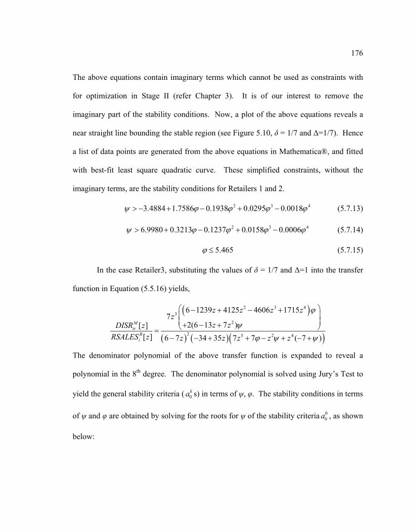
176

The above equations contain imaginary terms which cannot be used as constraints with

for optimization in Stage II (refer Chapter 3). It is of our interest to remove the

imaginary part of the stability conditions. Now, a plot of the above equations reveals a

near straight line bounding the stable region (see Figure 5.10, δ = 1/7 and ∆=1/7). Hence

a list of data points are generated from the above equations in Mathematica®, and fitted

with best-fit least square quadratic curve. These simplified constraints, without the

imaginary terms, are the stability conditions for Retailers 1 and 2.

2 33.4884 1.7586 0.1938 0.0295 0.0018 4ψ ϕ ϕ ϕ> − + − + − ϕ

4

(5.7.13)

2 36.9980 0.3213 0.1237 0.0158 0.0006ψ ϕ ϕ ϕ> + − + − ϕ (5.7.14)

5.465ϕ ≤ (5.7.15)

In the case Retailer3, substituting the values of δ = 1/7 and ∆=1 into the transfer

function in Equation (5.5.16) yields,

( )

( ) ( )( )

2 3 43

2

2 5 2 4

6 1239 4125 4606 17157

2(6 13 7 )[ ][ ] 6 7 34 35 7 7 ( 7 )

Mir

Ri

z z z zz

z zDISR zRSALES z z z z z z

ϕ

ψ

ϕ ψ ψ

⎛ ⎞− + − +⎜ ⎟⎜ ⎟+ − +⎝ ⎠=

− − + + − + − +



yield the general stability criteria ( s) in terms of ψ, φ. The stability conditions in terms

of ψ and φ are obtained by solving for the roots for ψ of the stability criteria , as shown

below:

0ka

00a

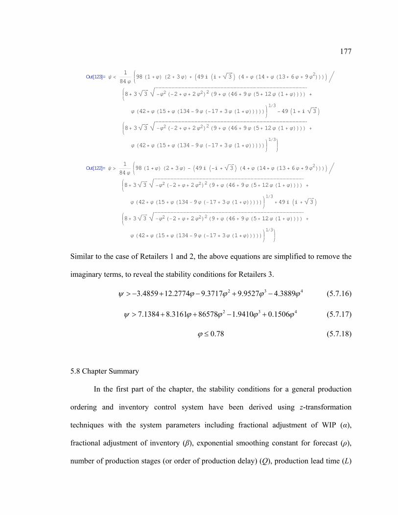
177

Out[123]= ψ <1

84ϕikjj98H1+ϕL H2+ 3ϕL + I49 I +

è!!!!3M H4+ ϕ H14+ ϕ H13+ 6ϕ + 9ϕ2LLLM ì

ikjj8+ 3è!!!!3 "###### ## #### ## ## ## #### ## ## ## #### ## ## ## #### ## ## ## #### ## ## ## #### #### ## #### #### ## ## ## #### ## ## ## #

−ϕ2H−2+ ϕ+ 2ϕ2L2H9+ ϕ H46+ 9ϕ H5+ 12ϕ H1+ ϕLLLL +


−49I1+ è!!!!3M

ikjj8+ 3è!!!!3 "###### ## #### ## ## ## #### ## ## ## #### ## ## ## #### ## ## ## #### ## ## ## #### #### ## #### #### ## ## ## #### ## ## ## #



Out[122]= ψ >1

84ϕikjj98H1+ϕL H2+ 3ϕL − I49 I− +

è!!!!3M H4+ ϕ H14+ ϕ H13+ 6ϕ +9ϕ2LLLM ì

ikjj8+ 3è!!!!3 "######## ## ## ## ## ## ## ## ## ## ## ## ## ## ## ## ## ## ## ## ## ## ## ## ## ## ## ## ## ## ## ## ## ## ## ## ## ## ## ## ## ## ## #



+49 I +è!!!!3M

ikjj8+ 3è!!!!3 "######## ## ## ## ## ## ## ## ## ## ## ## ## ## ## ## ## ## ## ## ## ## ## ## ## ## ## ## ## ## ## ## ## ## ## ## ## ## ## ## ## ## ## #



4

Similar to the case of Retailers 1 and 2, the above equations are simplified to remove the

imaginary terms, to reveal the stability conditions for Retailers 3.

2 33.4859 12.2774 9.3717 9.9527 4.3889ψ ϕ ϕ ϕ> − + − + − ϕ

4

(5.7.16)

2 37.1384 8.3161 86578 1.9410 0.1506ψ ϕ ϕ ϕ> + + − + ϕ (5.7.17)

0.78ϕ ≤ (5.7.18)

5.8 Chapter Summary

In the first part of the chapter, the stability conditions for a general production

ordering and inventory control system have been derived using z-transformation

techniques with the system parameters including fractional adjustment of WIP (α),

fractional adjustment of inventory (β), exponential smoothing constant for forecast (ρ),

number of production stages (or order of production delay) (Q), production lead time (L)

178

and the sampling interval (δ). The stability boundaries for system operating under

inventory adequacy and inventory insufficiency have been established. The system

response measured is the production release order quantities (PREL). The Jury’s Test has

been employed to derive the stability conditions for the PREL transfer function whose

characteristic polynomial is a higher order polynomial.

The effect of the frequency of information update on the stability of the

production-inventory system has also been analyzed. Results have revealed that

aggressive ordering policies (higher values of the fractional adjustment rates for WIP and

inventory) require a more frequent information update, i.e. lower sampling interval. Also,

the stable Deziel-Eilon settings of the fractional adjustment rates have been found to be

dependent on the sampling interval, stressing the need to select the appropriate control

parameters also based on the sampling interval.

In the second part of the chapter, a collaborative supply chain configuration

employing vendor managed inventory has been modeled and analyzed. Stability

conditions have been derived using z-transform technique with the system parameters

including adjustment rate for goods-in-transit (ψ), adjustment rates for inventory levels at

Retailers (φ), exponential smoothing constant for forecasting demand (ρ), time to change

the MIN and MAX levels (τ), the product delivery lead time and the sampling intervals (δ

and ∆). The system response measured is the dispatch order quantities (DISR). The

Jury’s Test has been employed to derive the stability conditions for the DISR transfer

function whose characteristic polynomial is a higher order polynomial.

179

Next, the possible differences in the frequency of information update at the

different players and their effect on overall system stability have been analyzed. The

stability conditions in terms of ψ and φ are obtained by mapping the frequency of

information update to the sampling intervals of Manufacturer (δ) and Retailer (∆). For

the case in which δ = ∆, it is found that the sampling interval settings of 1/7 (daily

updates) presents the largest stability region, thus allowing for a more aggressive

ordering policy, and the sampling interval settings of 1 (weekly updates) allows for a

very cautious ordering policy. It is also found that frequent updates of information on the

side of the Retailer (∆ < δ) alone improves system wide performance (larger stability

region). Also, even when the Manufacturer makes updates more frequent than the

Retailers (∆ > δ) they gains no advantage as their decisions are based on obsolete

information from the Retailer. Hence it is desirable and could be cost effective for the

Manufacturer to pace their decisions equal or slower than the rate at which the Retailers

can update the information.

In Section 5.5, stability conditions for each player of the supply chain are

obtained. These conditions are suited to the supply chain scenario described in Section

3.5 and the parameters presented in Section 4.7. The stability conditions for the

Manufacturer’s product production management are presented in Equations (5.7.1)-

(5.7.4); the Manufacturer’s component ordering are presented in Equations (5.7.4)-

(5.7.8); the Supplier’s component production management are presented in Equations

(5.7.9)-(5.7.12); the collaborative management of Retailer’s inventory are presented in

Equations (5.7.13)-(5.7.18).

180

CHAPTER 6

INTEGRATED PERFORMANCE AND STABILITY ANALYSIS OF

SUPPLY CHAIN PLANNING (STAGE II)

In this chapter the optimal sets of control parameters for use in the decision

policies of the model are determined using non-linear dynamic optimization techniques.

A novel method for the integration of the stability analysis with performance analysis

(optimization) is presented by employing the stability conditions derived in the previous

chapter as additional constraints within the optimization models. The need for such

integration is emphasized through preliminary experiments.

6.1 Background on System Dynamics Optimization

The use of optimization with system dynamics model can be broadly classified

into two areas (Dangerfield and Roberts 1996): (1) calibration of the model parameters to

obtain a reasonable fit of the model to past data, (2) determination of the model

parameters to improve certain system performance criteria. The latter is of interest in this

research. For the supply chain scenario considered, it is desirable to minimize the total

cost in the face of unknown demand. In this context, the optimization is used to

determine how the parameters associated with the control of inventory and the control of

WIP (or supply line), should be set in order that the total cost is minimized.

Typically, optimization is achieved by combining the system dynamics (SD)

simulation model and optimization search routines (or optimizer). In each iteration SD

181

simulation model determines the value of the objective function, which is given to the

optimizer. The optimizer, using on its search routines, chooses the parameter values that

might improve the objective function, which is given to the SD simulation models to test

the resultant improvement in the objective function. The search routines within the

optimizer consists of hill-climbing algorithms such as genetic algorithm, tabu search

scatter search etc.

Now, it is recalled that the system dynamics models are governed by the

underlying difference equations (Chapters 4 and 5). Inspection of the equations reveals a

dynamic programming model with multiple non-linear constraints. Hence, in this

research, the non-linear dynamic programming model (or the system dynamics model) is

optimized directly using the non-linear solver MINOS 5.5. MINOS uses a sparse SLC

algorithm (a projected augmented Lagrangian algorithm). It solves a sequence of sub

problems in which the constraints are linearized and the objective is an augmented

Lagrangian (involving all nonlinear functions). MINOS treats the linear constraints

specifically, but the non-linear constraints may not be satisfied until an optimal point is

reached. For further details on the algorithm kindly refer Murtagh and Saunders (1998).

Based on the proposed architecture (Chapter 3) and its applicability to the supply

chain scenario (Chapter 3), the Supplier models are optimized separately while the

Manufacturer and Retailer models are optimized in a collaborative configuration, as

shown in Figure 6.1. These optimization activities are performed as part of the Step II

activities in the proposed architecture. The optimal sets of control parameters for use in

the decision policies of the respective model are determined using non-linear dynamic

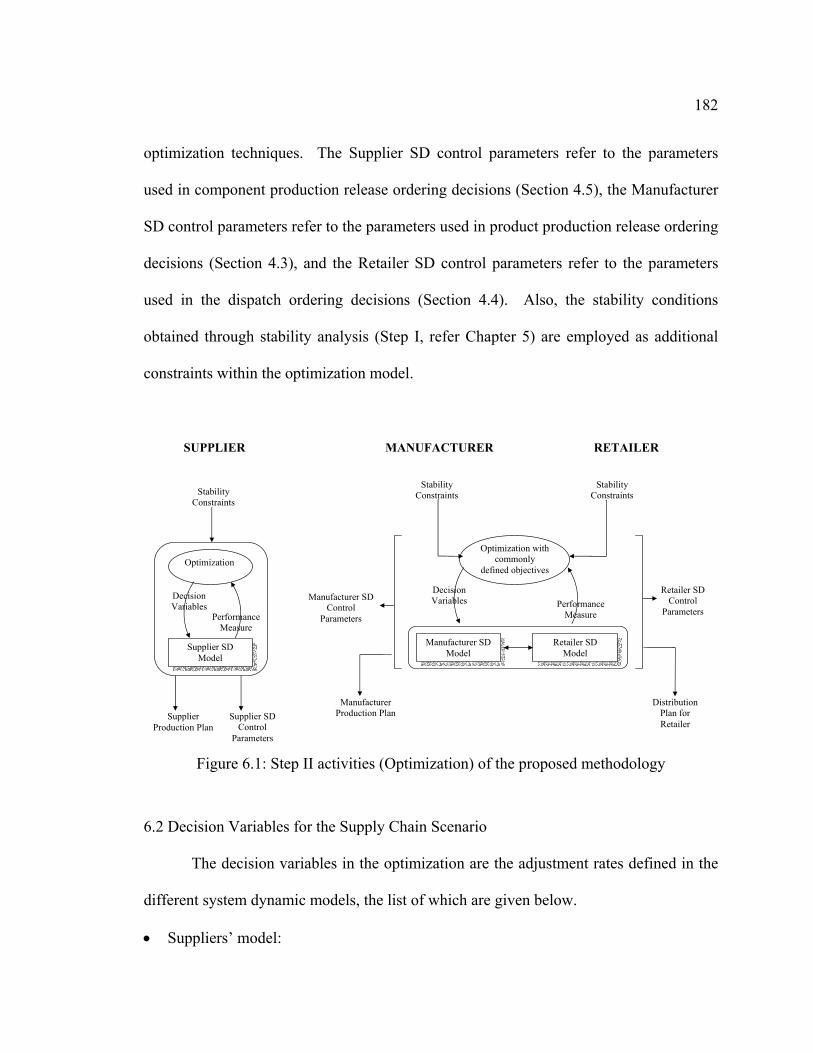
182

optimization techniques. The Supplier SD control parameters refer to the parameters

used in component production release ordering decisions (Section 4.5), the Manufacturer

SD control parameters refer to the parameters used in product production release ordering

decisions (Section 4.3), and the Retailer SD control parameters refer to the parameters

used in the dispatch ordering decisions (Section 4.4). Also, the stability conditions

obtained through stability analysis (Step I, refer Chapter 5) are employed as additional

constraints within the optimization model.


MANUFACTURER

Optimization

Decision Variables

Performance Measure

Supplier SD Model

Supplier SD Control

Parameters

Supplier Production Plan



defined objectives

Decision Variables



Manufacturer SD Control

Parameters

Manufacturer Production Plan

Performance Measure

Retailer SD Model

Retailer SD Control

Parameters

Distribution Plan for Retailer

SUPPLIER RETAILER

Figure 6.1: Step II activities (Optimization) of the proposed methodology

6.2 Decision Variables for the Supply Chain Scenario

The decision variables in the optimization are the adjustment rates defined in the

different system dynamic models, the list of which are given below.

• Suppliers’ model:

183

o Fractional adjustment rates of component WIP ( Sjα )

o Fractional adjustment rates of component inventory ( Sjβ )

• Manufacturer’s model:

o Fractional adjustment rates of product WIP ( Miα )

o Fractional adjustment rates of product inventory ( Miβ )

o Fractional adjustment rates of component supply GIT ( Miγ )

o Fractional adjustment rates of component inventory ( Miη )

o Fractional adjustment rates of Retailer product GIT ( Miψ )

o Fractional adjustment rates of Retailer inventory ( Miϕ )

It is noted that Miψ and M

iϕ are the Retailer SD control parameters indicated in Figure 6.1.

The other parameters in the models such as production lead time, exponential smoothing

forecast constant, supply lead etc require knowledge of the system, and hence are set

based on the calculations and assumptions presented in Sections 4.7 and 5.7.

6.3 Objective Functions for the Supply Chain Scenario

Cost-based objective function is used in the optimization in this research. It is

desired to minimize the total cost. Typical cost function for the aggregate production

planning function includes the production costs, inventory holding costs and inventory

shortage costs. This function is adequate in the case of Material Requirements Planning

(MRP) type aggregate planning problems, where the production quantity for each time

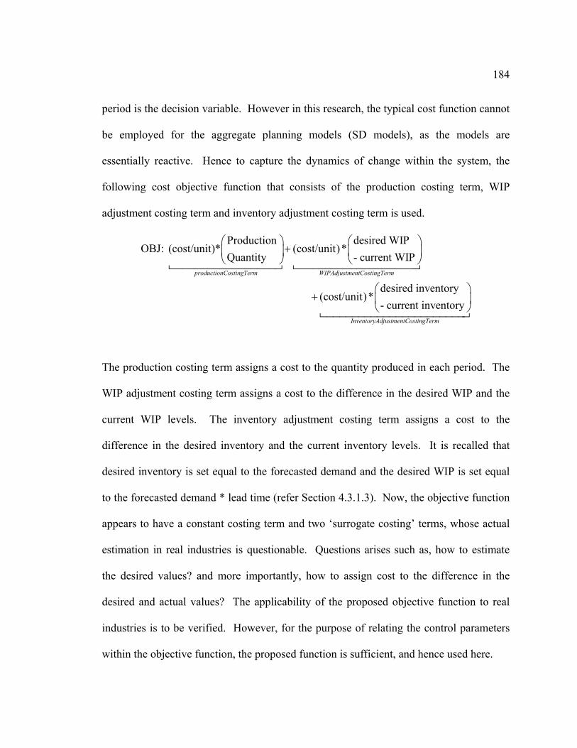
184

period is the decision variable. However in this research, the typical cost function cannot

be employed for the aggregate planning models (SD models), as the models are

essentially reactive. Hence to capture the dynamics of change within the system, the

following cost objective function that consists of the production costing term, WIP

adjustment costing term and inventory adjustment costing term is used.

Production desired WIPOBJ: (cost/unit)* (cost/unit)*

Quantity - current WIP

desired inventory(cost/unit)*

-

productionCostingTerm WIPAdjustmentCostingTerm

⎛ ⎞ ⎛ ⎞+⎜ ⎟ ⎜ ⎟

⎝ ⎠ ⎝ ⎠

+current inventory

InventoryAdjustmentCostingTerm

⎛ ⎞⎜ ⎟⎝ ⎠

The production costing term assigns a cost to the quantity produced in each period. The

WIP adjustment costing term assigns a cost to the difference in the desired WIP and the

current WIP levels. The inventory adjustment costing term assigns a cost to the

difference in the desired inventory and the current inventory levels. It is recalled that

desired inventory is set equal to the forecasted demand and the desired WIP is set equal

to the forecasted demand * lead time (refer Section 4.3.1.3). Now, the objective function

appears to have a constant costing term and two ‘surrogate costing’ terms, whose actual

estimation in real industries is questionable. Questions arises such as, how to estimate

the desired values? and more importantly, how to assign cost to the difference in the

desired and actual values? The applicability of the proposed objective function to real

industries is to be verified. However, for the purpose of relating the control parameters

within the objective function, the proposed function is sufficient, and hence used here.

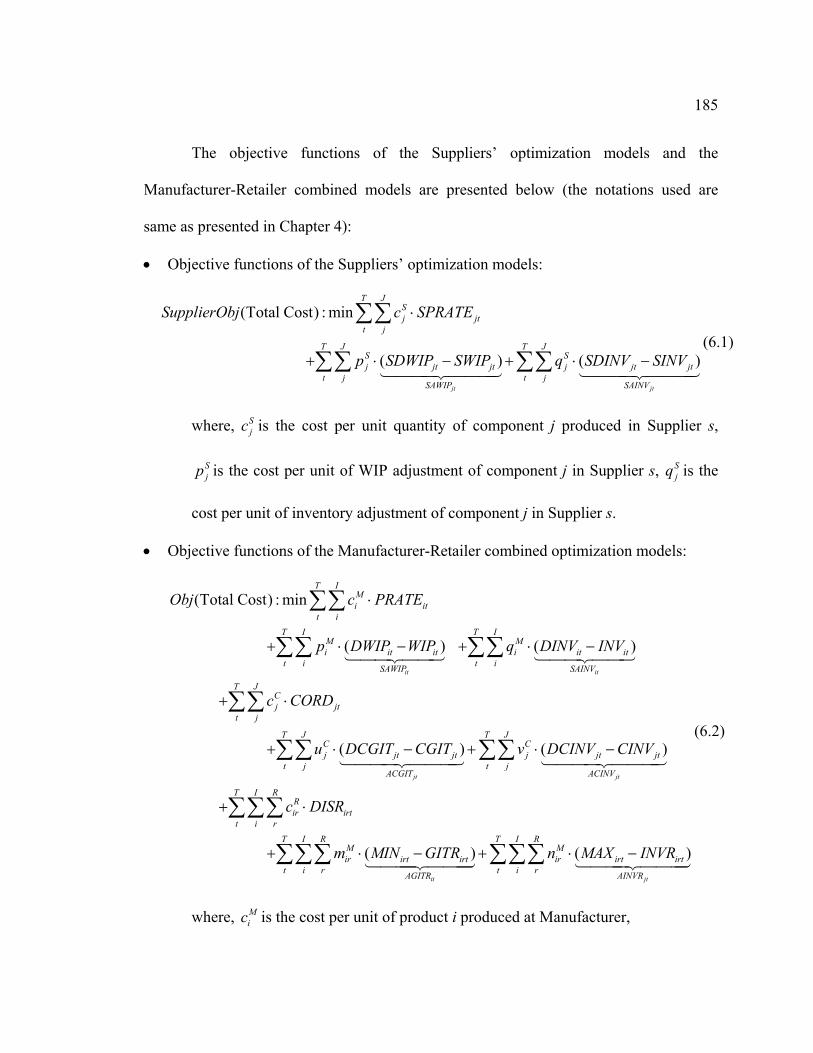
185

The objective functions of the Suppliers’ optimization models and the

Manufacturer-Retailer combined models are presented below (the notations used are

same as presented in Chapter 4):

• Objective functions of the Suppliers’ optimization models:

(Total Cost) : min

( ) (jt jt

T JSj jt

t j

T J T JS Sj jt jt j jt

t j t jSAWIP SAINV

SupplierObj c SPRATE

)jtp SDWIP SWIP q SDINV SINV

⋅

+ ⋅ − + ⋅ −

∑∑

∑∑ ∑∑(6.1)

where, is the cost per unit quantity of component j produced in Supplier s, Sjc

Sjp is the cost per unit of WIP adjustment of component j in Supplier s, is the

cost per unit of inventory adjustment of component j in Supplier s.

Sjq

• Objective functions of the Manufacturer-Retailer combined optimization models:

(Total Cost) : min

( ) ( )

( ) (

it it

jt

T IMi it

t iT I T I

M Mi it it i it it

t i t iSAWIP SAINV

T JCj jt

t j

T JC Cj jt jt j jt jt

t jACGIT ACINV

Obj c PRATE

p DWIP WIP q DINV INV

c CORD

u DCGIT CGIT v DCINV CINV

⋅

+ ⋅ − + ⋅ −

+ ⋅

+ ⋅ − + ⋅ −

∑∑

∑∑ ∑∑

∑∑

∑∑

( ) (

jt

it jt

T J

t j

T I RRir irt

t i r

T I R T I RM Mir irt irt ir irt irt

t i r t i rAGITR AINVR

c DISR

m MIN GITR n MAX INVR

+ ⋅

+ ⋅ − + ⋅ −

∑∑

∑∑∑

∑∑∑ ∑∑∑

)

)

(6.2)

where, Mic is the cost per unit of product i produced at Manufacturer,

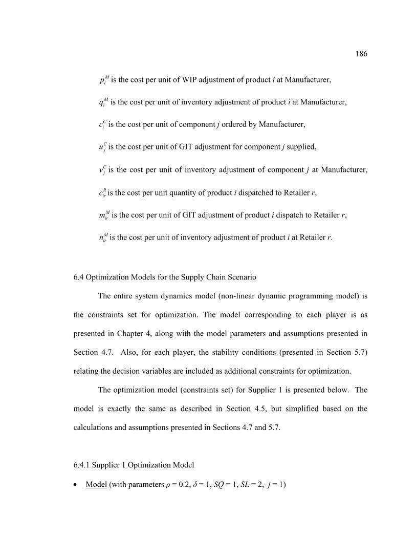
186

Mip is the cost per unit of WIP adjustment of product i at Manufacturer,

Miq is the cost per unit of inventory adjustment of product i at Manufacturer,

Cic is the cost per unit of component j ordered by Manufacturer,

Cju is the cost per unit of GIT adjustment for component j supplied,

Cjv is the cost per unit of inventory adjustment of component j at Manufacturer,

is the cost per unit quantity of product i dispatched to Retailer r, Rirc

Mirm is the cost per unit of GIT adjustment of product i dispatch to Retailer r,

Mirn is the cost per unit of inventory adjustment of product i at Retailer r.

6.4 Optimization Models for the Supply Chain Scenario

The entire system dynamics model (non-linear dynamic programming model) is

the constraints set for optimization. The model corresponding to each player is as

presented in Chapter 4, along with the model parameters and assumptions presented in

Section 4.7. Also, for each player, the stability conditions (presented in Section 5.7)

relating the decision variables are included as additional constraints for optimization.

The optimization model (constraints set) for Supplier 1 is presented below. The

model is exactly the same as described in Section 4.5, but simplified based on the

calculations and assumptions presented in Sections 4.7 and 5.7.

6.4.1 Supplier 1 Optimization Model

• Model (with parameters ρ = 0.2, δ = 1, SQ = 1, SL = 2, j = 1)

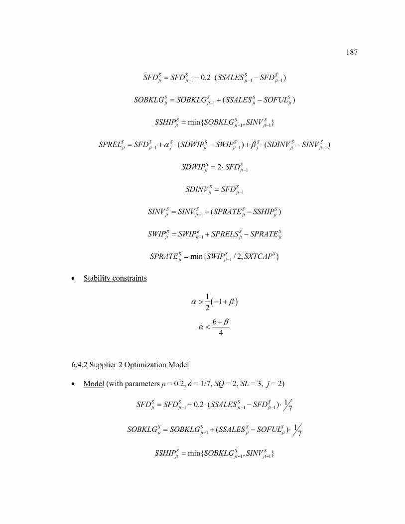
187

1 10.2 ( )S S S Sjt jt jt jtSFD SFD SSALES SFD 1− −= + ⋅ − −

)S

1S−

1)S−

S

1 (S S Sjt jt jt jtSOBKLG SOBKLG SSALES SOFUL−= + −

1min{ , }S Sjt jt jtSSHIP SOBKLG SINV−=

1 1( ) (S S S S S S Sjt jt j jt jt j jt jtSPREL SFD SDWIP SWIP SDINV SINVα β− −= + ⋅ − + ⋅ −

12Sjt jtSDWIP SFD −= ⋅

1Sjt jtSDINV SFDS

−=

1 (S S Sjt jt jt jtSINV SINV SPRATE SSHIP−= + − )S

S

S

1R R Sjt jt jt jtSWIP SWIP SPRELS SPRATE−= + −

1min{ / 2, }S Sjt jtSPRATE SWIP SXTCAP−=

• Stability constraints

(1 12

)α β> − +

64βα +

<

6.4.2 Supplier 2 Optimization Model

• Model (with parameters ρ = 0.2, δ = 1/7, SQ = 2, SL = 3, j = 2)

1 110.2 ( ) 7

S S S Sjt jt jt jtSFD SFD SSALES SFD− −= + ⋅ − ⋅1−

11( 7

S S S Sjt jt jt jtSOBKLG SOBKLG SSALES SOFUL− )= + − ⋅

1S−

1min{ , }S Sjt jt jtSSHIP SOBKLG SINV−=

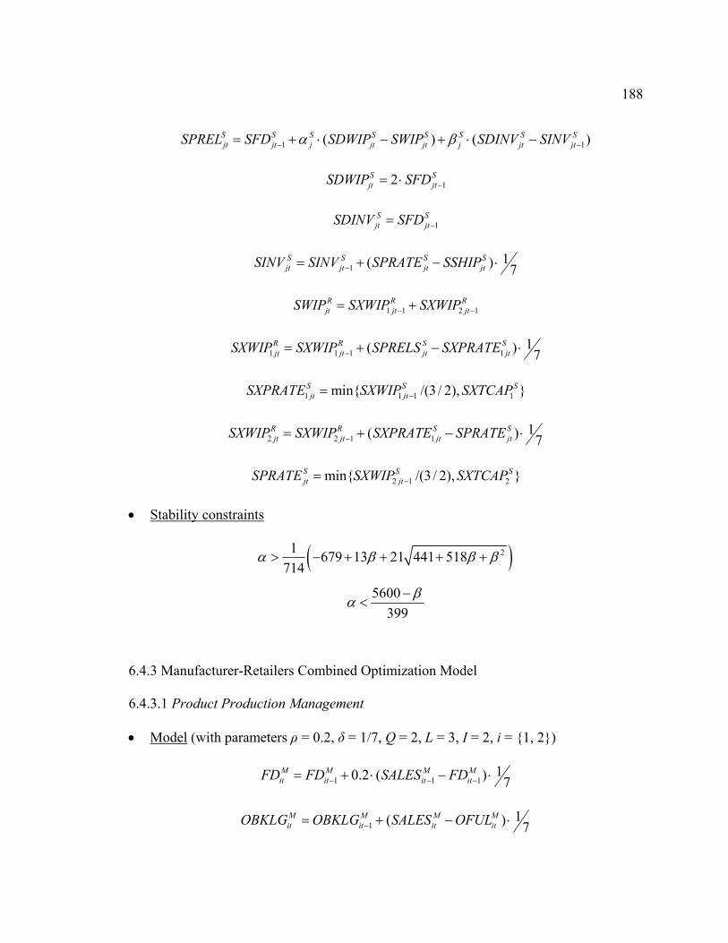
188

1 1( ) (S S S S S S Sjt jt j jt jt j jt jtSPREL SFD SDWIP SWIP SDINV SINVα β− −= + ⋅ − + ⋅ − )S

S 12Sjt jtSDWIP SFD −= ⋅

1Sjt jtSDINV SFDS

−=

11( 7

S S S Sjt jt jt jtSINV SINV SPRATE SSHIP− )= + − ⋅

R

1 1 2 1R Rjt jt jtSWIP SXWIP SXWIP− −= +

1 1 1 11( 7

R R S Sjt jt jt jtSXWIP SXWIP SPRELS SXPRATE−= + − ) ⋅

1S

1 1 1min{ /(3 / 2), }S Sjt jtSXPRATE SXWIP SXTCAP−=

2 2 1 11( 7

R R S Sjt jt jt jtSXWIP SXWIP SXPRATE SPRATE−= + − ) ⋅

S

2 1 2min{ /(3 / 2), }S Sjt jtSPRATE SXWIP SXTCAP−=


( )21 679 13 21 441 518714

α β β> − + + + + β

5600399

βα −<

6.4.3 Manufacturer-Retailers Combined Optimization Model

6.4.3.1 Product Production Management

• Model (with parameters ρ = 0.2, δ = 1/7, Q = 2, L = 3, I = 2, i = {1, 2})

1 110.2 ( ) 7

M M M Mit it it itFD FD SALES FD− − 1−= + ⋅ − ⋅

11( 7

M M M Mit it it itOBKLG OBKLG SALES OFUL− )= + − ⋅

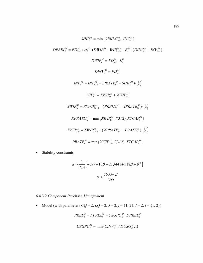
189

1min{ , ]M M Mit it itSHIP OBKLG INV−=

1 1( ) (M M M M M M M Mit it i it it i it itDPREL FD DWIP WIP DINV INVα β− −= + ⋅ − + ⋅ − 1)−

1M M M

it it itDWIP FD L−= ⋅

1M M

it itDINV FD −=

11( 7

M M M Mit it it itINV INV PRATE SHIP− )= + − ⋅

2

1M M

it it itWIP XWIP XWIP= + M

1 1 1 11( 7

M M M Mit it it itXWIP SXWIP PRELS XPRATE−= + − ) ⋅

1M

1 1 1min{ /(3 / 2), }M Mit itXPRATE XWIP XTCAP−=

2 2 1 11( 7

M M M Mit it it itXWIP XWIP XPRATE PRATE−= + − ) ⋅

M

2 1 2min{ /(3 / 2), }M Mit itPRATE XWIP XTCAP−=


( )21 679 13 21 441 518714

α β β> − + + + + β

5600399

βα −<

6.4.3.2 Component Purchase Management

• Model (with parameters CQ = 2, LQ = 2, J = 2, j = {1, 2}, I = 2, i = {1, 2})

M M Mit it jt itPREL FPREL USGPC DPREL= = ⋅ M

M

1min{ / ,1}M Mjt jt jtUSGPC CINV DUSG−=

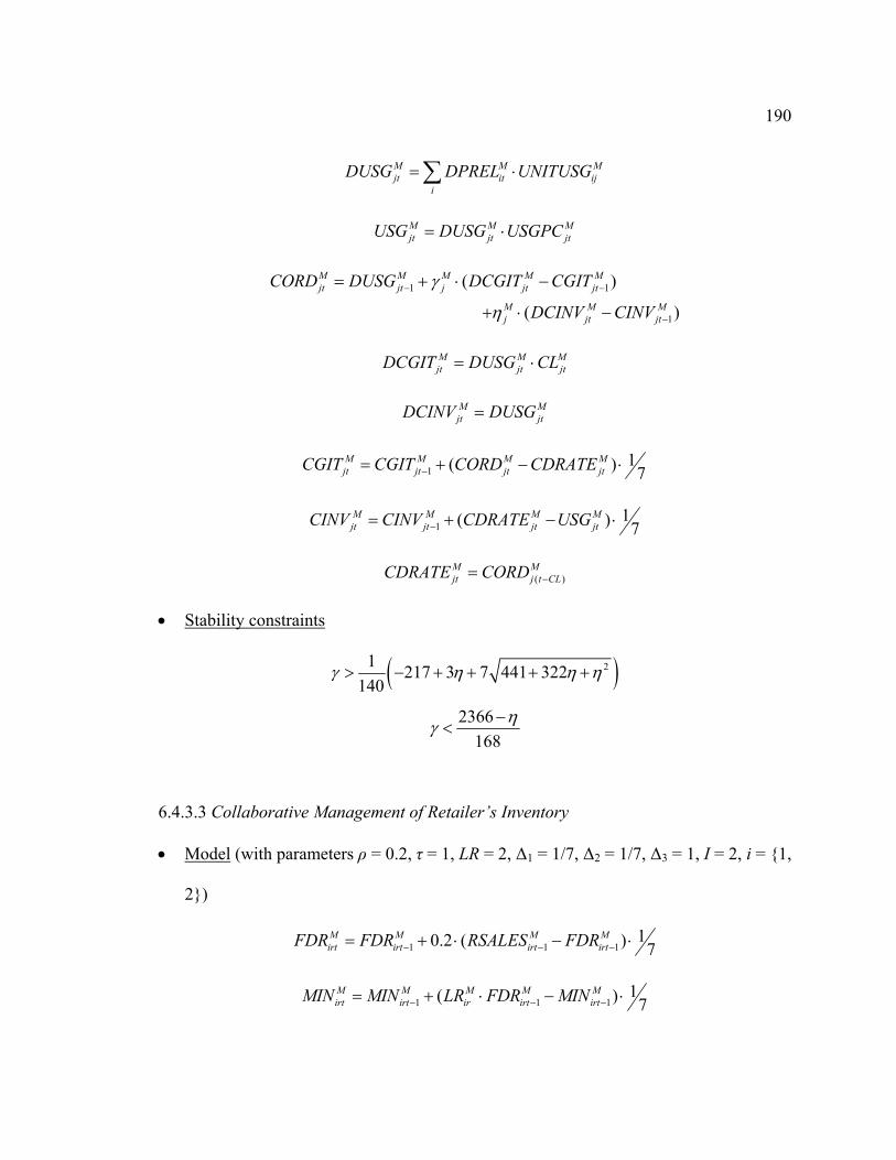
190

M Mjt it ij

iDUSG DPREL UNITUSG= ⋅ M∑

M Mjt jt jtUSG DUSG USGPC= ⋅ M

1

Mjt

−

1

1

( )

( )

M M M M Mjt jt j jt jt

M Mj jt

CORD DUSG DCGIT CGIT

DCINV CINV

γ

η−

−

= + ⋅ −

+ ⋅ −

M Mjt jt jtDCGIT DUSG CL= ⋅ M

M Mjt jtDCINV DUSG=

11( 7

M M M Mjt jt jt jtCGIT CGIT CORD CDRATE− )= + − ⋅

11( 7

M M M Mjt jt jt jtCINV CINV CDRATE USG− )= + − ⋅

)

(M Mjt j t CLCDRATE CORD −=


( )21 217 3 7 441 322140

γ η η> − + + + +η

2366168

ηγ −<

6.4.3.3 Collaborative Management of Retailer’s Inventory

• Model (with parameters ρ = 0.2, τ = 1, LR = 2, ∆1 = 1/7, ∆2 = 1/7, ∆3 = 1, I = 2, i = {1,

2})

1 110.2 ( ) 7

M M M Mirt irt irt irtFDR FDR RSALES FDR− −= + ⋅ − ⋅1−

1 11( 7

M M M M Mirt irt ir irt irtMIN MIN LR FDR MIN− −= + ⋅ − ⋅1)−

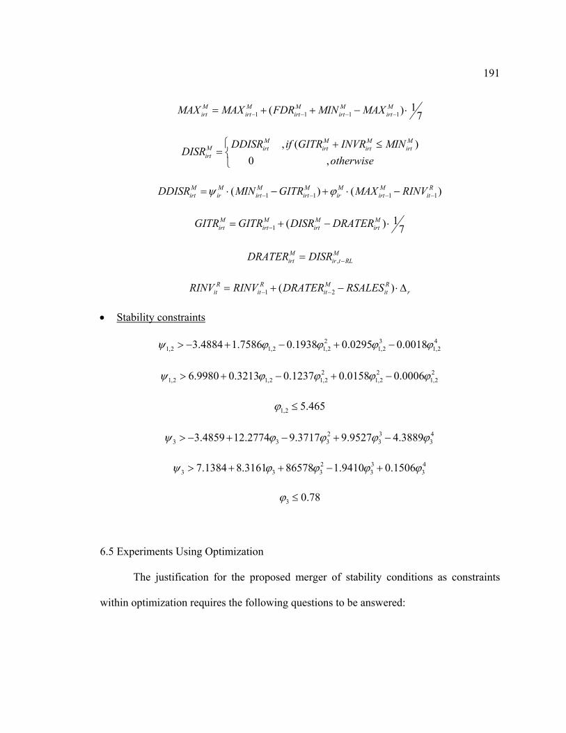
191

1 1 1 11( 7

M M M M Mirt irt irt irt irtMAX MAX FDR MIN MAX− − − −= + + − ⋅)

M

1)−

, ( )

0 ,



otherwise⎧ + ≤

= ⎨⎩

1 1 1( ) (M M M M M M Rirt ir irt irt ir irt itDDISR MIN GITR MAX RINVψ ϕ− − −= ⋅ − + ⋅ −

11( 7

M M M Mirt irt irt irtGITR GITR DISR DRATER− )= + − ⋅

,M Mirt ir t RLDRATER DISR −=

1 2(R R M Rit it it it rRINV RINV DRATER RSALES− −= + − ) ⋅∆


2 31,2 1,2 1,2 1,2 1,23.4884 1.7586 0.1938 0.0295 0.0018 4ψ ϕ ϕ ϕ ϕ> − + − + −

2 21,2 1,2 1,2 1,2 1,26.9980 0.3213 0.1237 0.0158 0.0006 2ψ ϕ ϕ ϕ ϕ> + − + −

1,2 5.465ϕ ≤

2 33 3 3 33.4859 12.2774 9.3717 9.9527 4.3889 4

3ψ ϕ ϕ ϕ> − + − + − ϕ

43

2 33 3 3 37.1384 8.3161 86578 1.9410 0.1506ψ ϕ ϕ ϕ> + + − + ϕ

3 0.78ϕ ≤

6.5 Experiments Using Optimization

The justification for the proposed merger of stability conditions as constraints

within optimization requires the following questions to be answered:

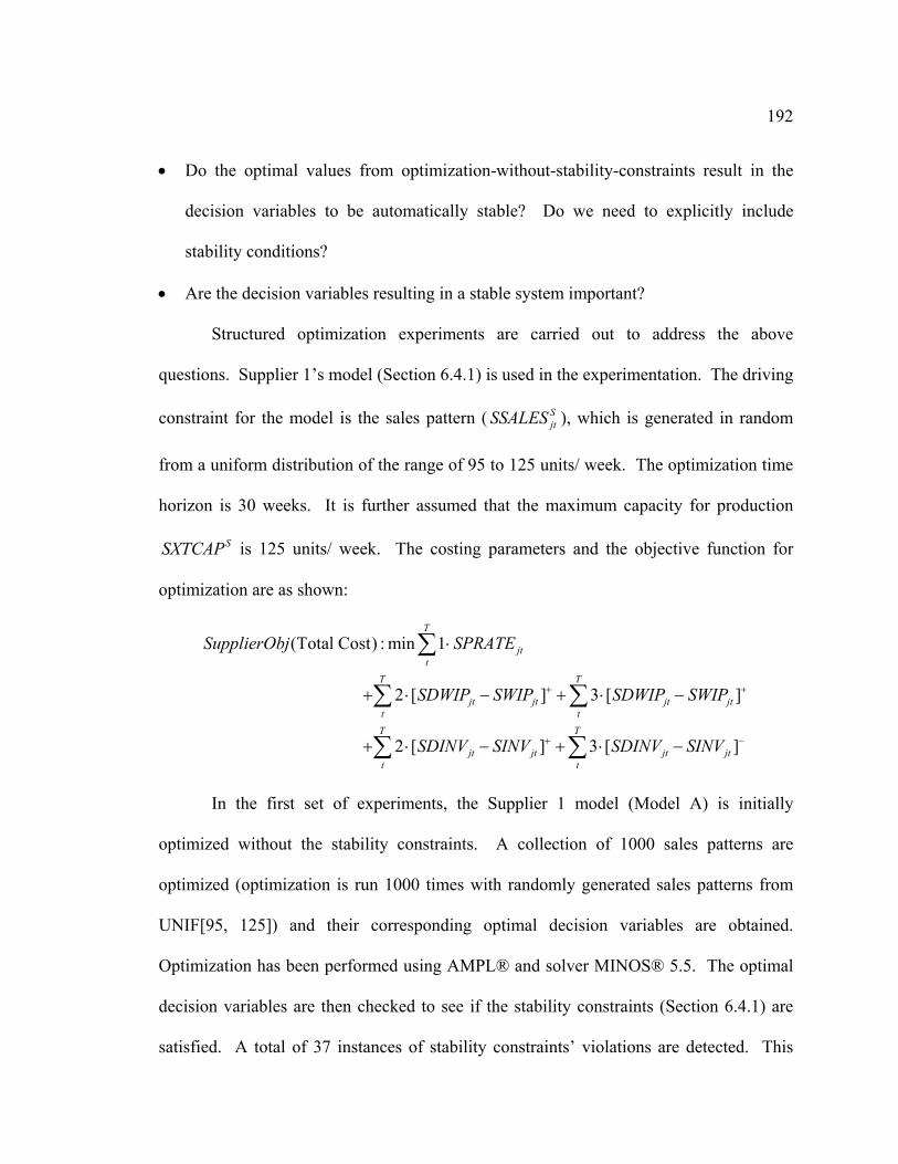
192

• Do the optimal values from optimization-without-stability-constraints result in the

decision variables to be automatically stable? Do we need to explicitly include

stability conditions?

• Are the decision variables resulting in a stable system important?

Structured optimization experiments are carried out to address the above

questions. Supplier 1’s model (Section 6.4.1) is used in the experimentation. The driving

constraint for the model is the sales pattern ( ), which is generated in random

from a uniform distribution of the range of 95 to 125 units/ week. The optimization time

horizon is 30 weeks. It is further assumed that the maximum capacity for production

is 125 units/ week. The costing parameters and the objective function for

optimization are as shown:

SjtSSALES

SSXTCAP

(Total Cost) : min 1

2 [ ] 3 [ ]

2 [ ] 3 [ ]

T

jtt

T T

jt jt jt jtt t

T T

jt jt jt jtt t

SupplierObj SPRATE

SDWIP SWIP SDWIP SWIP

SDINV SINV SDINV SINV

+ +

+ −

⋅

+ ⋅ − + ⋅ −

+ ⋅ − + ⋅ −

∑

∑ ∑

∑ ∑

In the first set of experiments, the Supplier 1 model (Model A) is initially

optimized without the stability constraints. A collection of 1000 sales patterns are

optimized (optimization is run 1000 times with randomly generated sales patterns from

UNIF[95, 125]) and their corresponding optimal decision variables are obtained.

Optimization has been performed using AMPL® and solver MINOS® 5.5. The optimal

decision variables are then checked to see if the stability constraints (Section 6.4.1) are

satisfied. A total of 37 instances of stability constraints’ violations are detected. This

193

confirms that the optimal decision variables selected are not always stable. The Supplier

1 model (Model B) is next optimized with the stability constraints. Now, the sales

patterns that had resulted in the optimal decision variables outside the stable region using

Model A, are used for optimization with Model B. It can be expected that the

optimization of Model B (with stability constraints) should result in the decision variables

within the stable region albeit higher total cost. Based on the optimization experiments,

20 of the 37 sales patterns resulted in stable decision variables with higher total costs, as

per our expectations. Interestingly, the remaining 15 of the 37 sales patterns resulted in a

total cost lower than that obtained using Model A. This belies the expectations that when

additional constraints are employed (the search space is reduced) there can be no

improvements to the objective. It is recalled that the models (Models A and B) employed

for optimization are highly non-linear and the MINOS® solver is based on a hill-

climbing algorithm. Given the nature of hill-climbing algorithms and the fact that they

do not guarantee global optimality, it is reasoned that the total cost objective obtained

using Model A is a local optimal. It is noted that such locally optimal results can be

improved by using different starting point, or improved algorithm. Now, the remaining 2

of the 37 sales patterns had resulted in critically stable decision variables in Model A, and

hence their values (and the objective) remain unchanged for Model B. Hence, it is

concluded that the stability conditions should be included as constraints within the non-

linear optimization model because: (1) absence of stability constraints in optimization can

result in the selection of unstable parameters, and (2) the efficiency of the non-linear

solver improves when stability conditions are included since the search space becomes

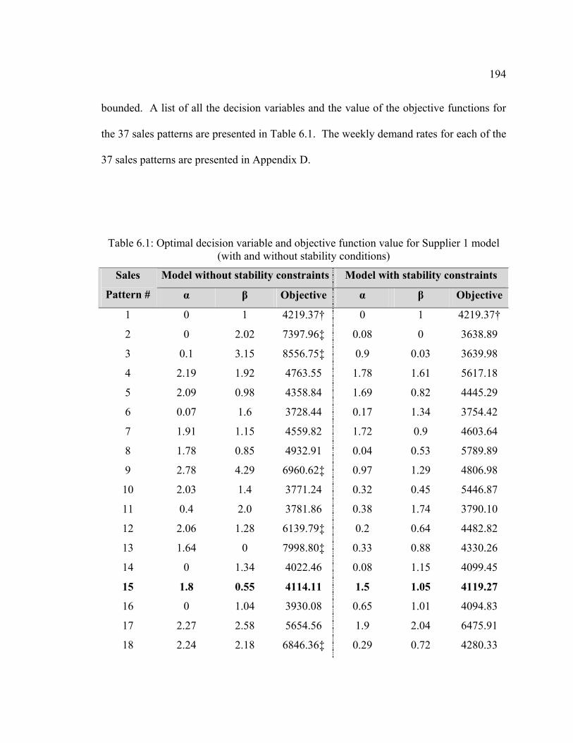
194

bounded. A list of all the decision variables and the value of the objective functions for

the 37 sales patterns are presented in Table 6.1. The weekly demand rates for each of the

37 sales patterns are presented in Appendix D.

Table 6.1: Optimal decision variable and objective function value for Supplier 1 model (with and without stability conditions)

Model without stability constraints Model with stability constraints Sales

Pattern # α β Objective α β Objective

1 0 1 4219.37† 0 1 4219.37†

2 0 2.02 7397.96‡ 0.08 0 3638.89

3 0.1 3.15 8556.75‡ 0.9 0.03 3639.98

4 2.19 1.92 4763.55 1.78 1.61 5617.18

5 2.09 0.98 4358.84 1.69 0.82 4445.29

6 0.07 1.6 3728.44 0.17 1.34 3754.42

7 1.91 1.15 4559.82 1.72 0.9 4603.64

8 1.78 0.85 4932.91 0.04 0.53 5789.89

9 2.78 4.29 6960.62‡ 0.97 1.29 4806.98

10 2.03 1.4 3771.24 0.32 0.45 5446.87

11 0.4 2.0 3781.86 0.38 1.74 3790.10

12 2.06 1.28 6139.79‡ 0.2 0.64 4482.82

13 1.64 0 7998.80‡ 0.33 0.88 4330.26

14 0 1.34 4022.46 0.08 1.15 4099.45

15 1.8 0.55 4114.11 1.5 1.05 4119.27

16 0 1.04 3930.08 0.65 1.01 4094.83

17 2.27 2.58 5654.56 1.9 2.04 6475.91

18 2.24 2.18 6846.36‡ 0.29 0.72 4280.33

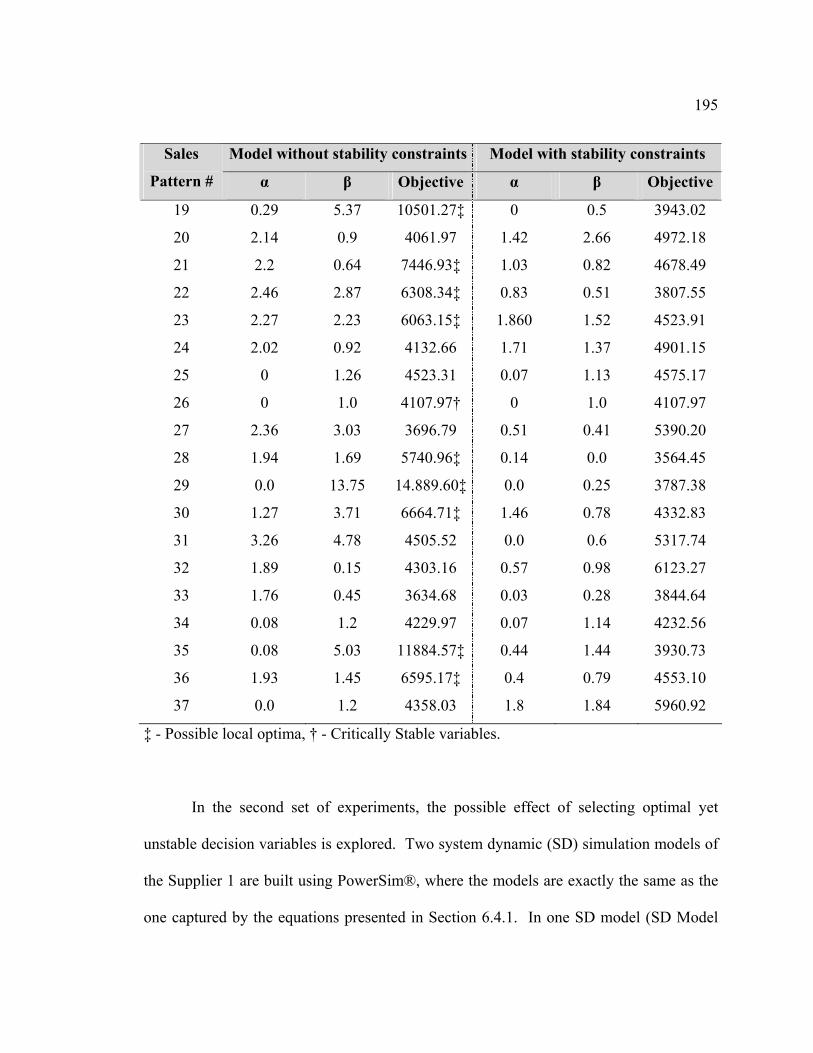
195

Model without stability constraints Model with stability constraints Sales

Pattern # α β Objective α β Objective

19 0.29 5.37 10501.27‡ 0 0.5 3943.02

20 2.14 0.9 4061.97 1.42 2.66 4972.18

21 2.2 0.64 7446.93‡ 1.03 0.82 4678.49

22 2.46 2.87 6308.34‡ 0.83 0.51 3807.55

23 2.27 2.23 6063.15‡ 1.860 1.52 4523.91

24 2.02 0.92 4132.66 1.71 1.37 4901.15

25 0 1.26 4523.31 0.07 1.13 4575.17

26 0 1.0 4107.97† 0 1.0 4107.97

27 2.36 3.03 3696.79 0.51 0.41 5390.20

28 1.94 1.69 5740.96‡ 0.14 0.0 3564.45

29 0.0 13.75 14.889.60‡ 0.0 0.25 3787.38

30 1.27 3.71 6664.71‡ 1.46 0.78 4332.83

31 3.26 4.78 4505.52 0.0 0.6 5317.74

32 1.89 0.15 4303.16 0.57 0.98 6123.27

33 1.76 0.45 3634.68 0.03 0.28 3844.64

34 0.08 1.2 4229.97 0.07 1.14 4232.56

35 0.08 5.03 11884.57‡ 0.44 1.44 3930.73

36 1.93 1.45 6595.17‡ 0.4 0.79 4553.10

37 0.0 1.2 4358.03 1.8 1.84 5960.92

‡ - Possible local optima, † - Critically Stable variables.

In the second set of experiments, the possible effect of selecting optimal yet

unstable decision variables is explored. Two system dynamic (SD) simulation models of

the Supplier 1 are built using PowerSim®, where the models are exactly the same as the

one captured by the equations presented in Section 6.4.1. In one SD model (SD Model

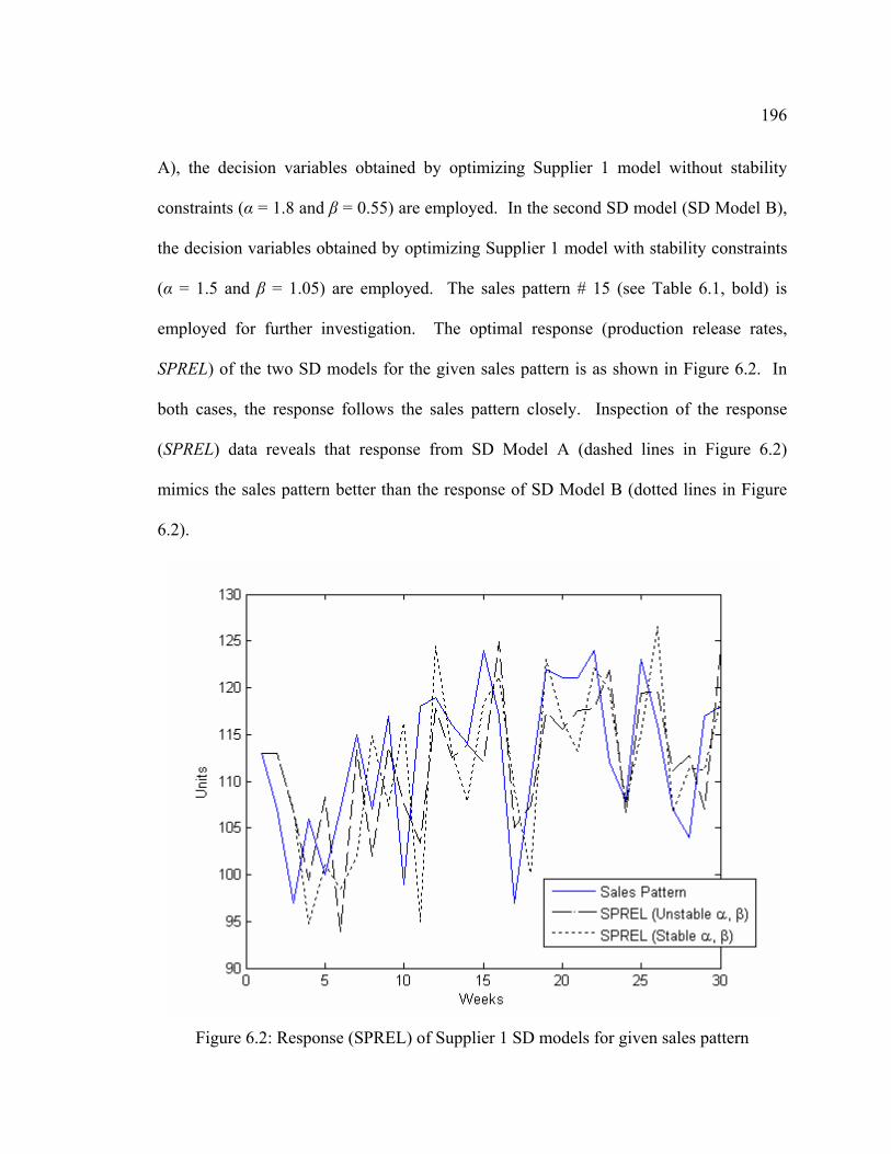
196

A), the decision variables obtained by optimizing Supplier 1 model without stability

constraints (α = 1.8 and β = 0.55) are employed. In the second SD model (SD Model B),

the decision variables obtained by optimizing Supplier 1 model with stability constraints

(α = 1.5 and β = 1.05) are employed. The sales pattern # 15 (see Table 6.1, bold) is

employed for further investigation. The optimal response (production release rates,

SPREL) of the two SD models for the given sales pattern is as shown in Figure 6.2. In

both cases, the response follows the sales pattern closely. Inspection of the response

(SPREL) data reveals that response from SD Model A (dashed lines in Figure 6.2)

mimics the sales pattern better than the response of SD Model B (dotted lines in Figure

6.2).

Figure 6.2: Response (SPREL) of Supplier 1 SD models for given sales pattern

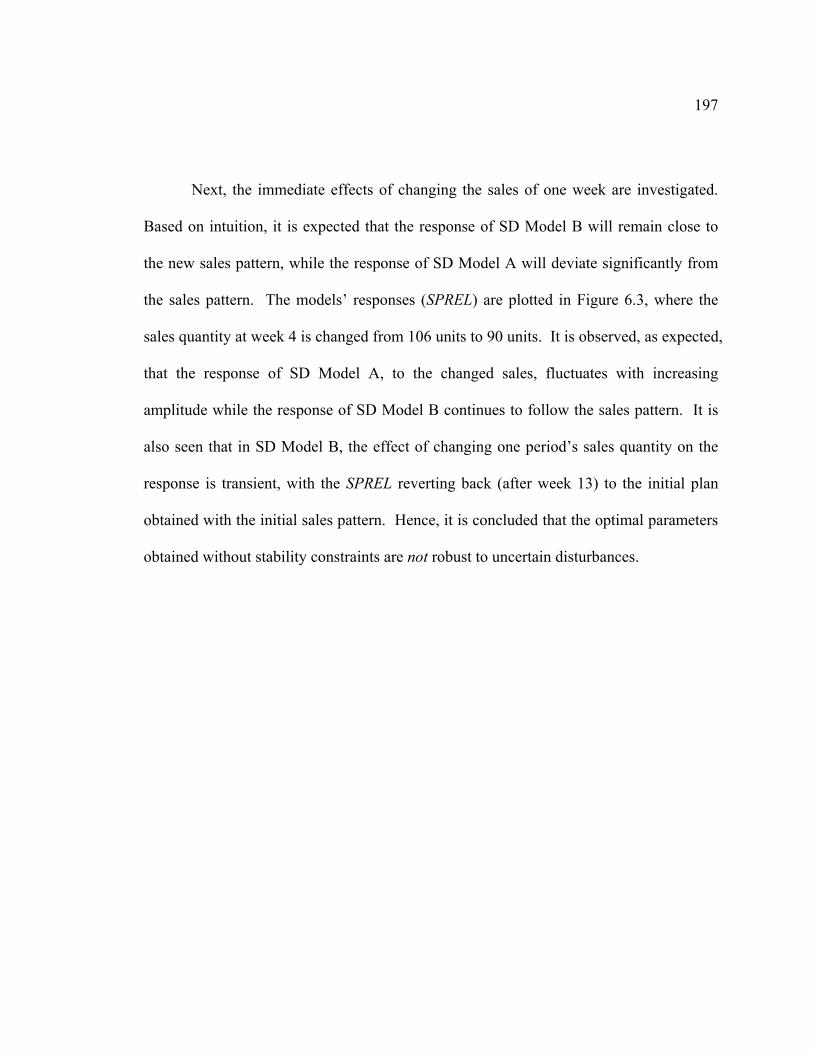
197

Next, the immediate effects of changing the sales of one week are investigated.

Based on intuition, it is expected that the response of SD Model B will remain close to

the new sales pattern, while the response of SD Model A will deviate significantly from

the sales pattern. The models’ responses (SPREL) are plotted in Figure 6.3, where the

sales quantity at week 4 is changed from 106 units to 90 units. It is observed, as expected,

that the response of SD Model A, to the changed sales, fluctuates with increasing

amplitude while the response of SD Model B continues to follow the sales pattern. It is

also seen that in SD Model B, the effect of changing one period’s sales quantity on the

response is transient, with the SPREL reverting back (after week 13) to the initial plan

obtained with the initial sales pattern. Hence, it is concluded that the optimal parameters

obtained without stability constraints are not robust to uncertain disturbances.

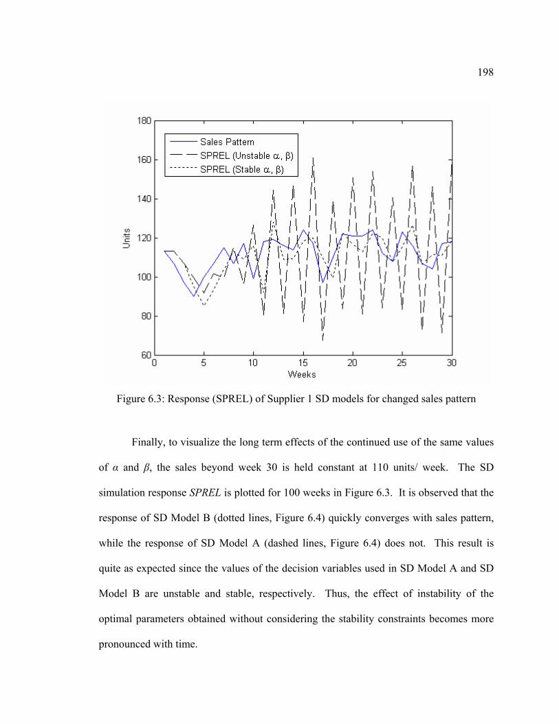
198

Figure 6.3: Response (SPREL) of Supplier 1 SD models for changed sales pattern

Finally, to visualize the long term effects of the continued use of the same values

of α and β, the sales beyond week 30 is held constant at 110 units/ week. The SD

simulation response SPREL is plotted for 100 weeks in Figure 6.3. It is observed that the

response of SD Model B (dotted lines, Figure 6.4) quickly converges with sales pattern,

while the response of SD Model A (dashed lines, Figure 6.4) does not. This result is

quite as expected since the values of the decision variables used in SD Model A and SD

Model B are unstable and stable, respectively. Thus, the effect of instability of the

optimal parameters obtained without considering the stability constraints becomes more

pronounced with time.

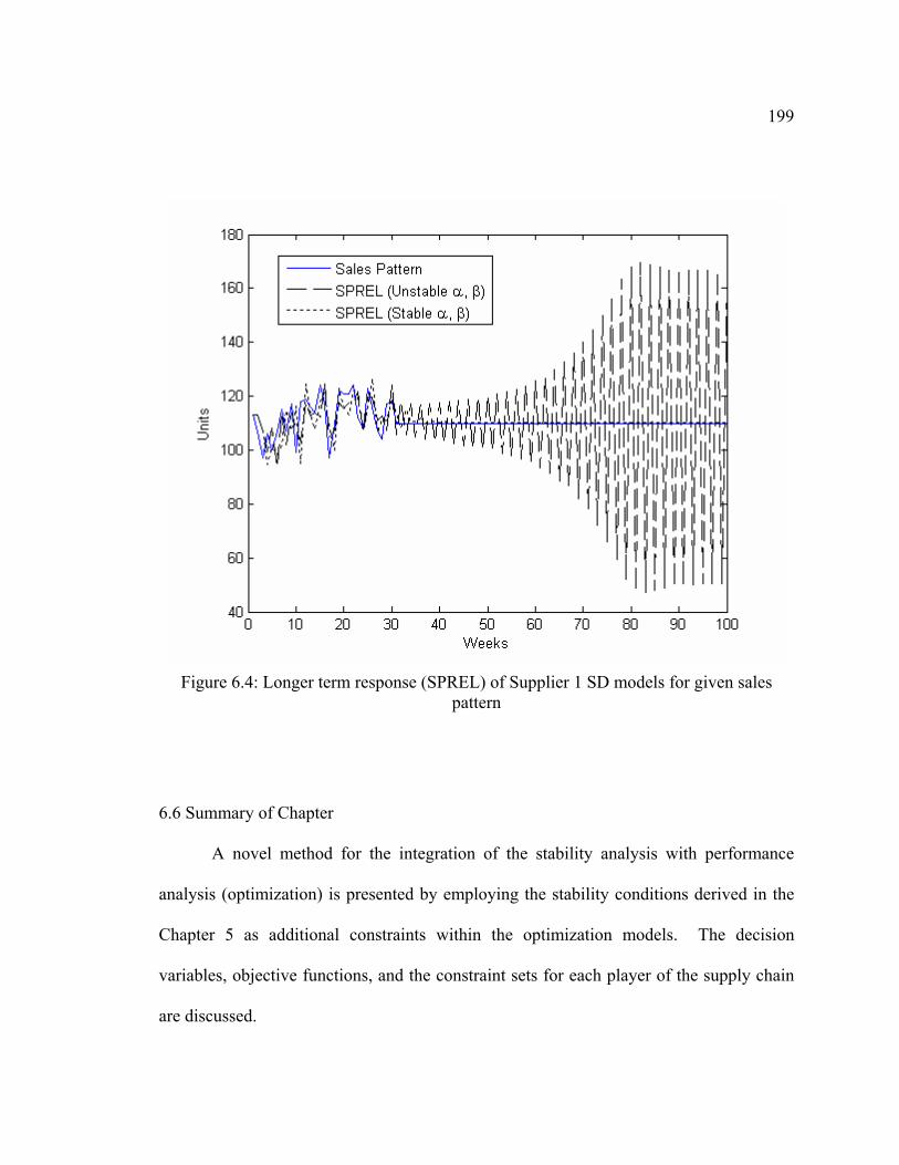
199

Figure 6.4: Longer term response (SPREL) of Supplier 1 SD models for given sales

pattern

6.6 Summary of Chapter

A novel method for the integration of the stability analysis with performance

analysis (optimization) is presented by employing the stability conditions derived in the

Chapter 5 as additional constraints within the optimization models. The decision

variables, objective functions, and the constraint sets for each player of the supply chain

are discussed.

200

Designed experiments using optimization has been carried out to justify the use of

stability constraints within the optimization model. AMPL® and solver MINOS® 5.5

were used to perform the optimization of the models. It is observed that optimization

could result in the selection of unstable set of decision variables which results in optimal

system response for a particular sales pattern. Based on the experiments, it is concluded

that the stability conditions should be included as constraints within the non-linear

optimization model because: (1) absence of stability constraints in optimization can result

in the selection of unstable parameters, and (2) the efficiency of the non-linear solver

improves when stability conditions are included since the search space becomes bounded.

Next, the adverse effects (short-term and long-term) of the use of such unstable variables

have been discussed. It is concluded that the optimal parameters obtained without

stability constraints are not robust to uncertain disturbances, and the effect of instability

becomes more pronounced with time.

The experimental results raise an interesting question: instead of using stability

constraints, can the system be optimized periodically? Now, periodic optimization could

possibly ensure that the effect of using unstable decision variables does not last longer

than the corresponding horizon. However, the success of periodic optimization depend

the length of the planning horizon and the frequency of re-optimization. Such decisions

can be greatly improved with the knowledge of the stability of system variables. The

investigation of the same is left as future research.

201

CHAPTER 7

INCLUSION OF DETAILED MODELS IN SUPPLY CHAIN ANALYSIS

(STAGES III AND IV)

In this chapter, the need for the inclusion of detailed models in supply chain

analysis is discussed. Description are presented for the modeling the detailed models

using Discrete Event Simulation (DES). Next, the schedule optimization (Stage III of the

proposed architecture) is described by presenting the decision variables, objective

functions and the optimization methodology. Finally, the specifications for interactions

of the SD and DES models, for use in Stage IV of the proposed architecture are detailed.

7.1 Development of the Detailed Models

In the proposed architecture and methodology, the detailed models (developed

using DES) are used in Stage III schedule optimization and Stage IV evaluation of the

optimal decisions. The detailed operational activities of the supply chain include

production within the factory shop, storage of goods, material flow internal to the factory

shop, and external transportation. In this research, separate DES models of the Suppliers,

Manufacturer, Transportation network and Retailers, are built. The rationale behind the

use of DES in representing the production and material flow activities are three fold:

• DES can describe the most complex manufacturing systems and include stochastic

elements, which cannot be described easily by mathematical or analytical models,

202

• DES allows one to track the status of individual entities and resources in the facility

and estimate numerous performance measures associated with those entities. These

properties are especially important for the detailed scheduling level, and

• With some modifications, DES can even use real-time data collected from the shop

floor or transportation network (Son et al. 2002).

Thus, DES is the best choice to model accurately the required level of detail to ensure

that the developed schedule is valid and the predetermined production plan can be met.

Furthermore, the models can be changed easily and run quickly to reflect changes that

occur in the actual system.

7.1.1 Description of the Discrete Event Simulation Models

The models of the members of the supply chain under study can be modeled and

simulated using scientific programming languages like C or C++. However, standard

simulation packages, like Arena®, ProModel®, AutoMod® etc, are available which ease

the building of models and provide support for output analysis and optimization. In favor

of advancing the author’s existing knowledge of Arena® 8.0 (Kelton et al. 1997, Kelton

et al. 2001), that simulation package is chosen for modeling the supply chain and

conducting the experiment.

Separate DES models are built using Arena 8.0 for the Suppliers, Manufacturer,

Transporter and Retailers, as per the specification and assumptions presented in Section

3.5. The DES models of the Manufacturer and Suppliers shops incorporates the detailed

shop operations including material processing, transfer and storage activities, along with

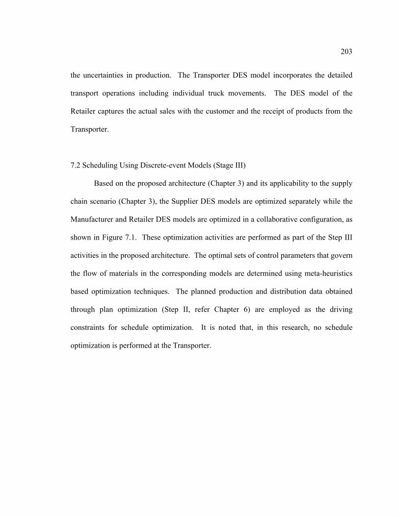
203

the uncertainties in production. The Transporter DES model incorporates the detailed

transport operations including individual truck movements. The DES model of the

Retailer captures the actual sales with the customer and the receipt of products from the

Transporter.

7.2 Scheduling Using Discrete-event Models (Stage III)

Based on the proposed architecture (Chapter 3) and its applicability to the supply

chain scenario (Chapter 3), the Supplier DES models are optimized separately while the

Manufacturer and Retailer DES models are optimized in a collaborative configuration, as

shown in Figure 7.1. These optimization activities are performed as part of the Step III

activities in the proposed architecture. The optimal sets of control parameters that govern

the flow of materials in the corresponding models are determined using meta-heuristics

based optimization techniques. The planned production and distribution data obtained

through plan optimization (Step II, refer Chapter 6) are employed as the driving

constraints for schedule optimization. It is noted that, in this research, no schedule

optimization is performed at the Transporter.

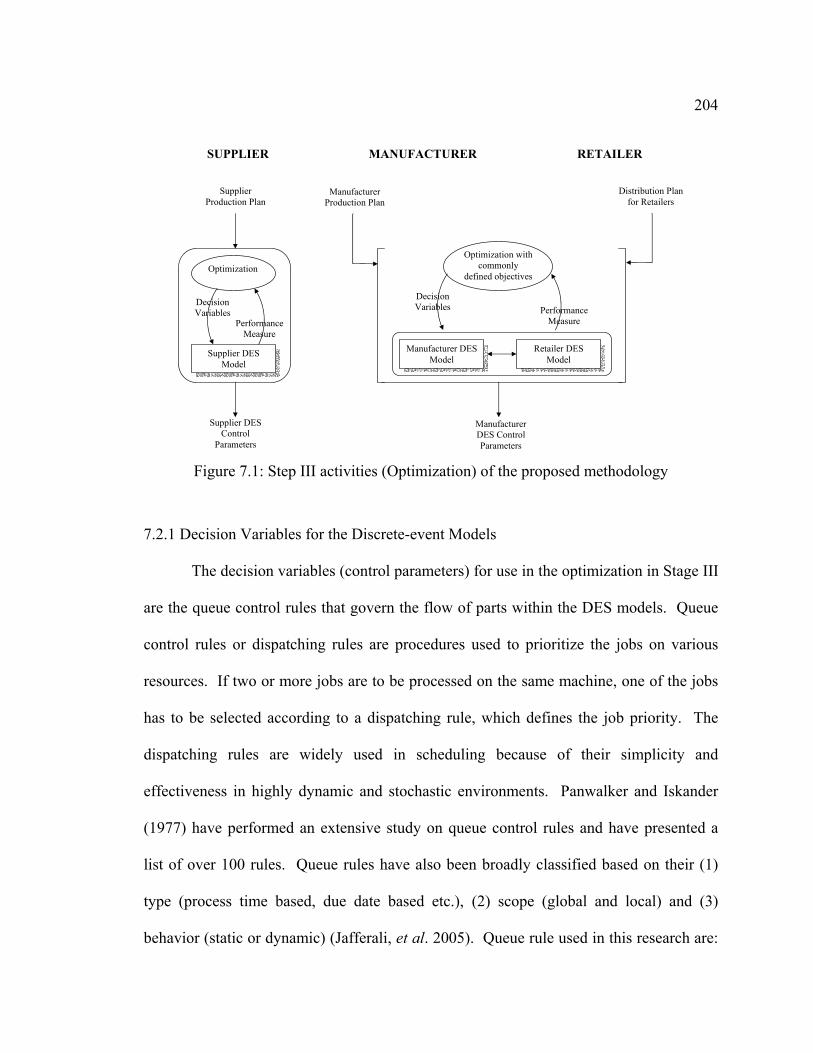
204

MANUFACTURER

Optimization

Decision Variables

Performance Measure

Supplier DES Model

Supplier DES Control

Parameters


defined objectives

Decision Variables



Manufacturer Production Plan

Performance Measure

Retailer DES Model

Distribution Plan for Retailers

SUPPLIER RETAILER

Supplier Production Plan

Figure 7.1: Step III activities (Optimization) of the proposed methodology

7.2.1 Decision Variables for the Discrete-event Models

The decision variables (control parameters) for use in the optimization in Stage III

are the queue control rules that govern the flow of parts within the DES models. Queue

control rules or dispatching rules are procedures used to prioritize the jobs on various

resources. If two or more jobs are to be processed on the same machine, one of the jobs

has to be selected according to a dispatching rule, which defines the job priority. The

dispatching rules are widely used in scheduling because of their simplicity and

effectiveness in highly dynamic and stochastic environments. Panwalker and Iskander

(1977) have performed an extensive study on queue control rules and have presented a

list of over 100 rules. Queue rules have also been broadly classified based on their (1)

type (process time based, due date based etc.), (2) scope (global and local) and (3)

behavior (static or dynamic) (Jafferali, et al. 2005). Queue rule used in this research are:

205

Shortest Processing Time (SPT), Longest Processing Time (LPT), Earliest Due Date

(EDD), First-In First-Out (FIFO), Last-in-First-Out (LIFO), and Priority Ordering (PO).

These queue rules are used in the scheduling at the Manufacturer and the Suppliers. It is

noted that there are no decision variables within the Retailer DES model.

7.2.2 Objective Function for the Discrete-event Models

The objective functions for use in schedule optimization of the factory shops

within the supply chain can be classified into (1) time-based, and (2) due-date based.

Time-based objectives includes makespan, flow time, non-value added time etc. Due-

date based objectives include mean tardiness, maximum lateness, number of tardy jobs

etc. Also, combinations of the multiple objectives are also popular.

In this research, the schedules are to be developed to satisfy the plan obtained

from Stage II. Hence, the objective function employed at the Manufacturer and Suppliers

is: percentage of the absolute difference in the planned and actual production quantity.

Actual production refers to the total quantity produced as obtained from the DES model.

7.2.3 Optimization Methodology

Optimization of schedule is performed based on the outputs of the stochastic

simulation models. This is known as simulation optimization (Fu 2001). In simulation

optimization, one or more discrete-event simulation models replace analytical objective

functions and constraints. The decision variables are the input to the simulation model,

and the performance or objective function values are the output of the simulation models

206

(see Figure 7.2). In each iteration, the DES model determines the value of the objective

function, which is then given to the optimization engine or optimizer. The optimizer

chooses the parameter values that might improve the objective function using its search

routines, which are then given to the DES models to test the resultant improvement in the

objective function. The search routines within the optimizer consist of hill-climbing

algorithms (or meta-heuristic algorithms) such as genetic algorithm, tabu search,

simulated annealing and neural networks. In this research Optquest® algorithm,

implemented as a combination of tabu search, scatter search and neural networks is used

(Glover et al. 1999). Details of the OptQuest® algorithm can be found in Glover et al.

(1999) and Jafferali et al. (2005).

Meta-heuristic Optimization (OptQuest)

Discrete-event Models (Arena)

Decision Variable

Objective

Figure 7.2: Simulation Optimization

7.3 Interactions of System Dynamic and Discrete-event Models (Stage IV)

In Stage IV, the feasibility of the optimal control parameters governing the

planning decisions (obtained from Stage II) and the detailed operational policies

governing the schedules (obtained from Stage III) are concurrently evaluated using

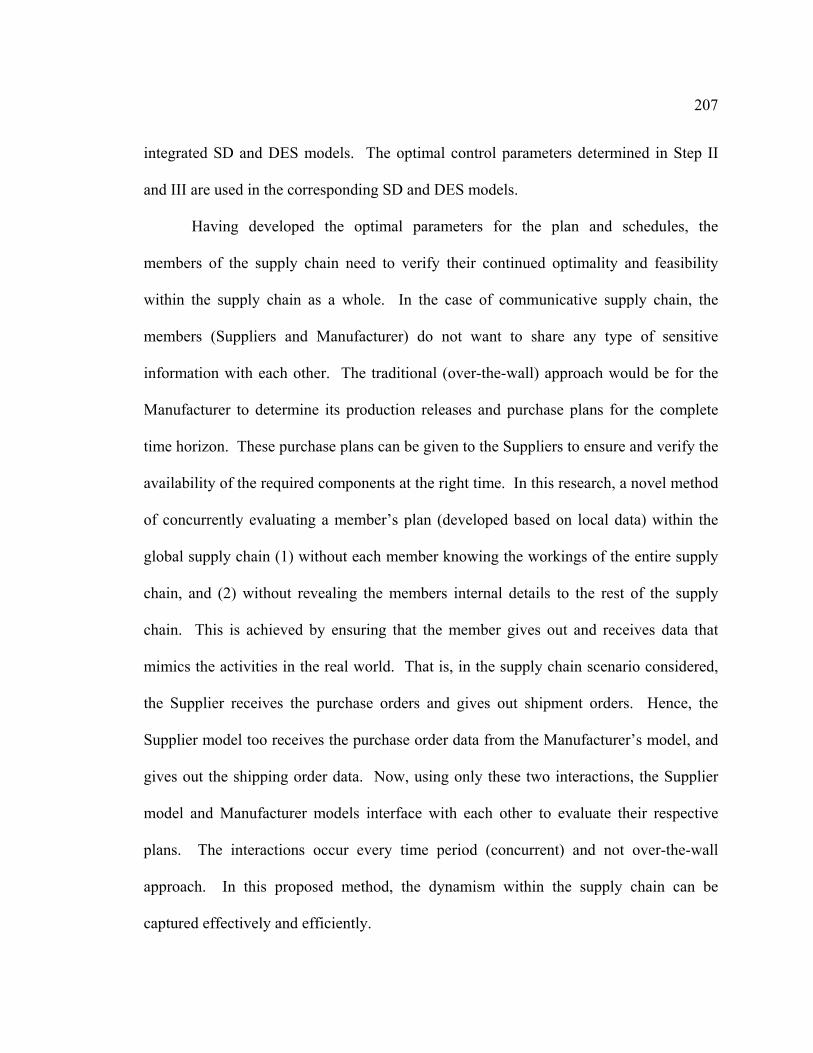
207

integrated SD and DES models. The optimal control parameters determined in Step II

and III are used in the corresponding SD and DES models.

Having developed the optimal parameters for the plan and schedules, the

members of the supply chain need to verify their continued optimality and feasibility

within the supply chain as a whole. In the case of communicative supply chain, the

members (Suppliers and Manufacturer) do not want to share any type of sensitive

information with each other. The traditional (over-the-wall) approach would be for the

Manufacturer to determine its production releases and purchase plans for the complete

time horizon. These purchase plans can be given to the Suppliers to ensure and verify the

availability of the required components at the right time. In this research, a novel method

of concurrently evaluating a member’s plan (developed based on local data) within the

global supply chain (1) without each member knowing the workings of the entire supply

chain, and (2) without revealing the members internal details to the rest of the supply

chain. This is achieved by ensuring that the member gives out and receives data that

mimics the activities in the real world. That is, in the supply chain scenario considered,

the Supplier receives the purchase orders and gives out shipment orders. Hence, the

Supplier model too receives the purchase order data from the Manufacturer’s model, and

gives out the shipping order data. Now, using only these two interactions, the Supplier

model and Manufacturer models interface with each other to evaluate their respective

plans. The interactions occur every time period (concurrent) and not over-the-wall

approach. In this proposed method, the dynamism within the supply chain can be

captured effectively and efficiently.

208

The DES models in Stage IV (this Stage), the exact same models as described in

Section 7 (built as per specification in Section 3.5) and used in Stage III (schedule

optimization). The SD models in this stage are almost the same model described in

Chapter 4, where the data for certain variables are now obtained from the DES models.

Thus the behavior of the entire supply chain is the result of complex inter-relationships

amongst the different models. The interactions between the SD and DES models, as

applicable to the supply chain scenario, are illustrated in Figure 7.3.

Demand Forecast

Production Order

Supplier SD Model

Supplier DES Model


Supplier SD Control

Parameters

Shop Status

Production Order

Manufacturer SD Model (Production Ordering)




Shop Status

Purchase Order

Component Delivery Receipt

Transporter DES Model


Manufacturer SD Model (Retailer’s Inventory

Mgmt)

Retailer DES Model

Retailers SD Control

Parameters

Dispatch Order

Inventory & Sales Data

Shipment Order

Product Delivery Receipt

Transport Status

A

B

C

D

E

F

G

H

Figure 7.3: Interactions between the SD and DES models in Stage IV

Detailed description of the models’ interactions is as follows:

• Marker A in Figure 7.3: The Supplier SD model obtains the current shop status

(component WIP, production lead time and inventory level data) from the Suppliers

209

shop DES model. Based on these data, the component production release order is

then calculated by the Supplier SD model, and sent to the Supplier DES model. The

DES model creates the corresponding component entities for production.

• Marker B in Figure 7.3: The component purchase orders are received by the Supplier

SD model from the Manufacturer’s SD model. Based on this order, the

corresponding shipment order is generated and sent to the Supplier DES model and

the Transporter DES model. On receiving the shipment order, the Supplier DES

model reduces its current inventory by the corresponding number; and the

Transporter DES model ‘creates’ the corresponding number of components for

transportation.

• Marker C in Figure 7.3: The Manufacturer SD model (production ordering) obtains

the current shop status (product WIP, production lead time and inventory level data)

from the Manufacturer shop DES model. Based on these data, the product production

release order is then calculated by the Manufacturer SD model, and sent to the

Manufacturer DES model. The DES model releases the corresponding entities for

production.

• Marker D in Figure 7.3: The Manufacturer SD model (production ordering) receives

the forecast demand data, used for production ordering, from the Retailers’ inventory

management SD model.

• Marker E in Figure 7.3: The component delivery receipts are sent from the

Transporter DES model to the Manufacturer shop DES model, to indicate that the

210

components have now reached the Manufacturer. The shop DES model updates the

component inventory levels.

• Marker F in Figure 7.3: The end customer sales data and the retailers’ inventory level

data are sent from the Retailer DES models to the Manufacturer SD model.

• Marker G in Figure 7.3: The goods-in-transit data and the transportation lead time

data are sent from the Transporter DES model to the Manufacturer SD model

(Retailers’ inventory management model). Based on the Retailer and Transporter

status data, the Manufacturer SD model determines the quantity to dispatch to the

Retailers. The dispatch order is then sent to the Manufacturer and Transporter DES

models. On receiving the dispatch order, the Manufacturer DES model reduces its

current inventory by the corresponding number; and the Transporter DES model

‘creates’ the corresponding number of products for transportation.

• Marker H in Figure 7.3: The product delivery receipts are sent from the Transporter

DES model to the Retailers DES model, to indicate that the products have now

reached the Retailers. The DES model updates the product inventory levels.

The interactions between the Manufacturer SD models with the DES models of the

Manufacturer, Retailer and Transporter is shown using a modified causal loop diagram in

Figure 7.4.

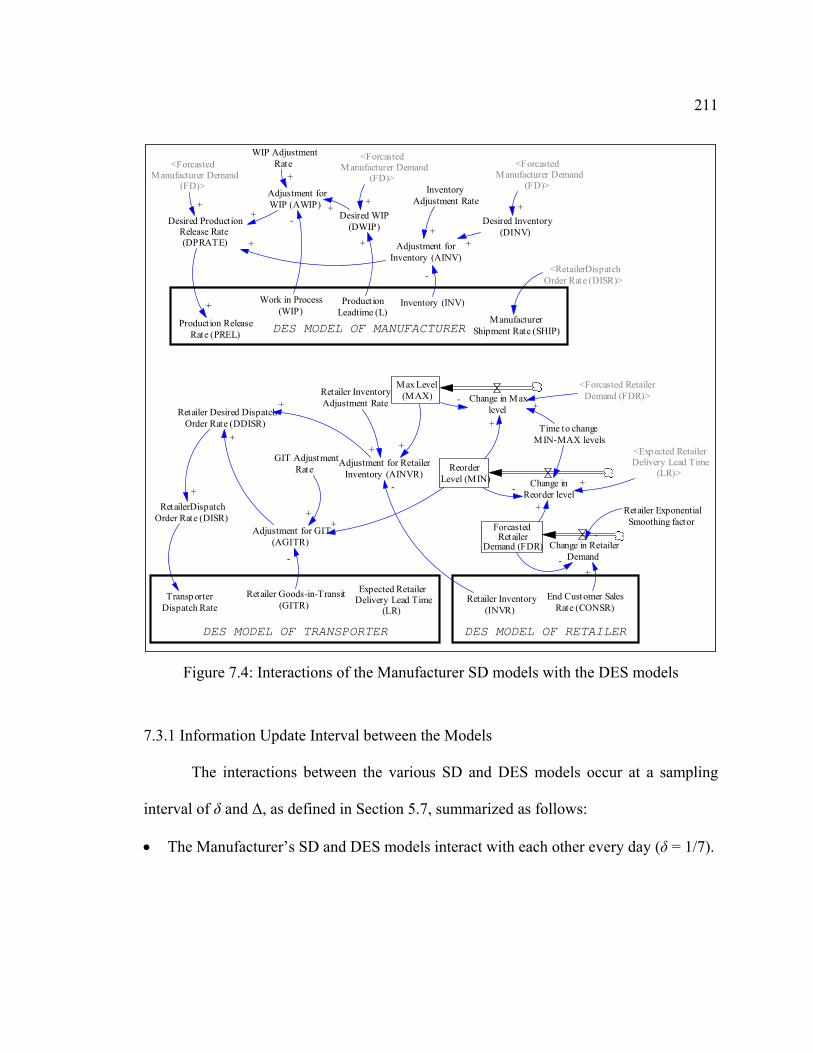
211





Desired WIP(DWIP)

+

+

+

+

WIP AdjustmentRate

+Inventory

Adjustment Rate

+

Product ionLeadtime (L)

+


(FD)>


(FD)><Forcasted


+ + +

ReorderLevel (MIN) Change in

Reorder level

Time to changeMIN-MAX levels

-

ForcastedRetailer

Demand (FDR) Change in RetailerDemand

Retailer ExponentialSmoothing factor

-

-

Max Level(MAX) Change in Max

level-

Retailer Desired DispatchOrder Rate (DDISR)

Expected RetailerDelivery Lead Time

(LR)

<Expected RetailerDelivery Lead Time

(LR)>+

Adjustment for GIT(AGITR)

Adjustment for RetailerInventory (AINVR)

+

+

GIT AdjustmentRate

Retailer InventoryAdjustment Rate

+

+

<Forcasted RetailerDemand (FDR)>

+

End Customer SalesRate (CONSR)

+

Retailer Inventory(INVR)

Product ion ReleaseRate (PREL)

Work in Process(WIP)

Inventory (INV)

ManufacturerShipment Rate (SHIP)

+

-

-

Retailer Goods-in-Transit(GITR)

RetailerDispatchOrder Rate (DISR) +

-

-

+

++

+

Transp orterDispatch Rate

<RetailerDispatchOrder Rate (DISR)>

DES MODEL OF MANUFACTURER

DES MODEL OF TRANSPORTER

DES MODEL OF RETAILER

Figure 7.4: Interactions of the Manufacturer SD models with the DES models

7.3.1 Information Update Interval between the Models

The interactions between the various SD and DES models occur at a sampling

interval of δ and ∆, as defined in Section 5.7, summarized as follows:

• The Manufacturer’s SD and DES models interact with each other every day (δ = 1/7).

212

• Also, Supplier 2’s SD and DES models interact with each other every day (δ = 1/7).

Supplier 2 SD model receives the purchase order from the Manufacturer’s SD model

in the same period as their sampling intervals are the same.

• Supplier 1’s SD and DES models interact with each other every week (δ = 1).

Supplier 1 SD model accumulates the purchase orders received from the

Manufacturer’s SD model in the previous week, and use it for its calculations in the

following week.

• The Manufacturer’s SD and Transporter DES model interact with each other every

day (δ = 1/7).

• The Manufacturer’s SD and Retailers (1 and 2) DES models interact with each other

every day (δ = 1/7).

• The Manufacturer’s SD and Retailers (3) DES models interact with each other every

week (δ = 1/7).

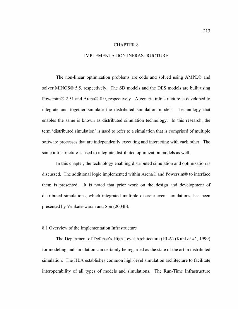
213

CHAPTER 8

IMPLEMENTATION INFRASTRUCTURE

The non-linear optimization problems are code and solved using AMPL® and

solver MINOS® 5.5, respectively. The SD models and the DES models are built using

Powersim® 2.51 and Arena® 8.0, respectively. A generic infrastructure is developed to

integrate and together simulate the distributed simulation models. Technology that

enables the same is known as distributed simulation technology. In this research, the

term ‘distributed simulation’ is used to refer to a simulation that is comprised of multiple

software processes that are independently executing and interacting with each other. The

same infrastructure is used to integrate distributed optimization models as well.

In this chapter, the technology enabling distributed simulation and optimization is

discussed. The additional logic implemented within Arena® and Powersim® to interface

them is presented. It is noted that prior work on the design and development of

distributed simulations, which integrated multiple discrete event simulations, has been

presented by Venkateswaran and Son (2004b).

8.1 Overview of the Implementation Infrastructure

The Department of Defense’s High Level Architecture (HLA) (Kuhl et al., 1999)

for modeling and simulation can certainly be regarded as the state of the art in distributed

simulation. The HLA establishes common high-level simulation architecture to facilitate

interoperability of all types of models and simulations. The Run-Time Infrastructure

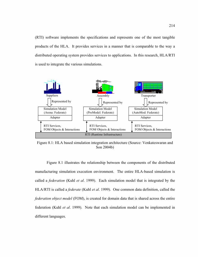
214

(RTI) software implements the specifications and represents one of the most tangible

products of the HLA. It provides services in a manner that is comparable to the way a

distributed operating system provides services to applications. In this research, HLA/RTI

is used to integrate the various simulations.

Represented by

Suppliers

RTI Services, FOM Objects & Interactions

Represented by

Assembly

Represented by

RTI (Runtime Infrastructure)

Simulation Model (Arena: Federate)

Adapter

Simulation Model (ProModel: Federate)

Adapter

Simulation Model (AutoMod: Federate)

Adapter



Transporter

Figure 8.1: HLA based simulation integration architecture (Source: Venkateswaran and

Son 2004b)

Figure 8.1 illustrates the relationship between the components of the distributed

manufacturing simulation execution environment. The entire HLA-based simulation is

called a federation (Kuhl et al. 1999). Each simulation model that is integrated by the

HLA/RTI is called a federate (Kuhl et al. 1999). One common data definition, called the

federation object model (FOM), is created for domain data that is shared across the entire

federation (Kuhl et al. 1999). Note that each simulation model can be implemented in

different languages.

215

Though the HLA RTI does provide a robust set of mechanisms for developing

distributed simulation, it is less suitable for use in a certain manufacturing domain. The

drawbacks include: (1) The direct interaction of the simulation federates with the RTI is

quite complex and cumbersome, (2) It has a steep learning curve for effective use, and (3)

It requires a significant amount of custom coding to develop distributed simulations from

simulation applications that were developed with the simulation tools that are common in

the manufacturing domain.

Hence, an interface called Distributed Manufacturing Simulation (DMS) Adapter

(referred to as ‘adapter’ in the rest of the document) has been developed “to provide

mechanisms for distributed simulation similar to those provided by the HLA RTI, but

with a level of complexity that is manageable by the development resources available in

the manufacturing community” (Riddick and McLean 2000). The DMS adapter provides

a simplified time management interface, automatic storage for local object instances,

management of lists of remote object instances, management and logging of interactions,

and simplified object and interact filtering.

8.2 Description of ‘Simulation Model — Adapter’ Interface

A generic interface module has been developed for use in Arena® (or any

discrete-event modeling package) and Powersim® (or any system dynamic modeling

package), so that simulation models in these languages can interface with the RTI via the

adapter. Since the developed interface modules are generic, the same modules have been

used for Suppliers (SD and DES), Manufacturers (SD and DES), Transporter (DES) and

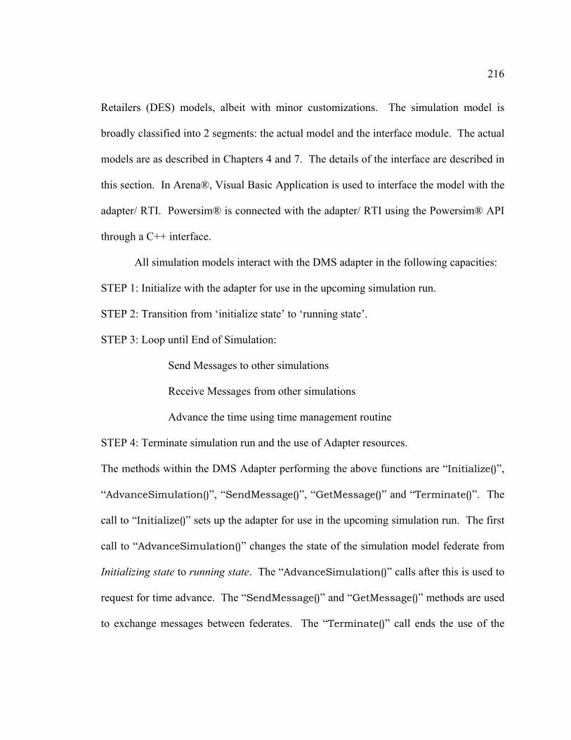
216

Retailers (DES) models, albeit with minor customizations. The simulation model is

broadly classified into 2 segments: the actual model and the interface module. The actual

models are as described in Chapters 4 and 7. The details of the interface are described in

this section. In Arena®, Visual Basic Application is used to interface the model with the

adapter/ RTI. Powersim® is connected with the adapter/ RTI using the Powersim® API

through a C++ interface.

All simulation models interact with the DMS adapter in the following capacities:

STEP 1: Initialize with the adapter for use in the upcoming simulation run.

STEP 2: Transition from ‘initialize state’ to ‘running state’.

STEP 3: Loop until End of Simulation:

Send Messages to other simulations

Receive Messages from other simulations

Advance the time using time management routine

STEP 4: Terminate simulation run and the use of Adapter resources.

The methods within the DMS Adapter performing the above functions are “Initialize()”,

“AdvanceSimulation()”, “SendMessage()”, “GetMessage()” and “Terminate()”. The

call to “Initialize()” sets up the adapter for use in the upcoming simulation run. The first

call to “AdvanceSimulation()” changes the state of the simulation model federate from

Initializing state to running state. The “AdvanceSimulation()” calls after this is used to

request for time advance. The “SendMessage()” and “GetMessage()” methods are used

to exchange messages between federates. The “Terminate()” call ends the use of the

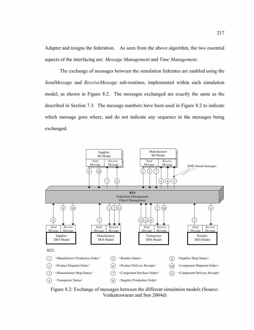
217

Adapter and resigns the federation. As seen from the above algorithm, the two essential

aspects of the interfacing are: Message Management and Time Management.

The exchange of messages between the simulation federates are enabled using the

SendMessage and ReceiveMessage sub-routines, implemented within each simulation

model, as shown in Figure 8.2. The messages exchanged are exactly the same as the

described in Section 7.3. The message numbers have been used in Figure 8.2 to indicate

which message goes where, and do not indicate any sequence in the messages being

exchanged.

Supplier SD Model

<Manufacturer Production Order>


Send Message

Receive Message

RTI Federation Management

Object Management

Send Message

Receive Message

Send Message

Receive Message

Send Message

Receive Message

Send Message

Receive Message

Send Message

Receive Message

1

XML-based messages

1

2

22

3

3

4

4 5

5

6

6

7

7

8

8

9

9

10

10 10

11

11

KEY:



Retailer DES Model

Supplier DES Model

1

2

3

4

5

7

6

11

8

9

10<Product Dispatch Order>

<Manufacturer Shop Status>

<Transporter Status>

<Retailer Status>

<Product Delivery Receipt>

<Component Purchase Order>

<Supplier Production Order>

<Supplier Shop Status>

<Component Shipment Order>

<Component Delivery Receipt>

Figure 8.2: Exchange of messages between the different simulation models (Source:

Venkateswaran and Son 2004d)

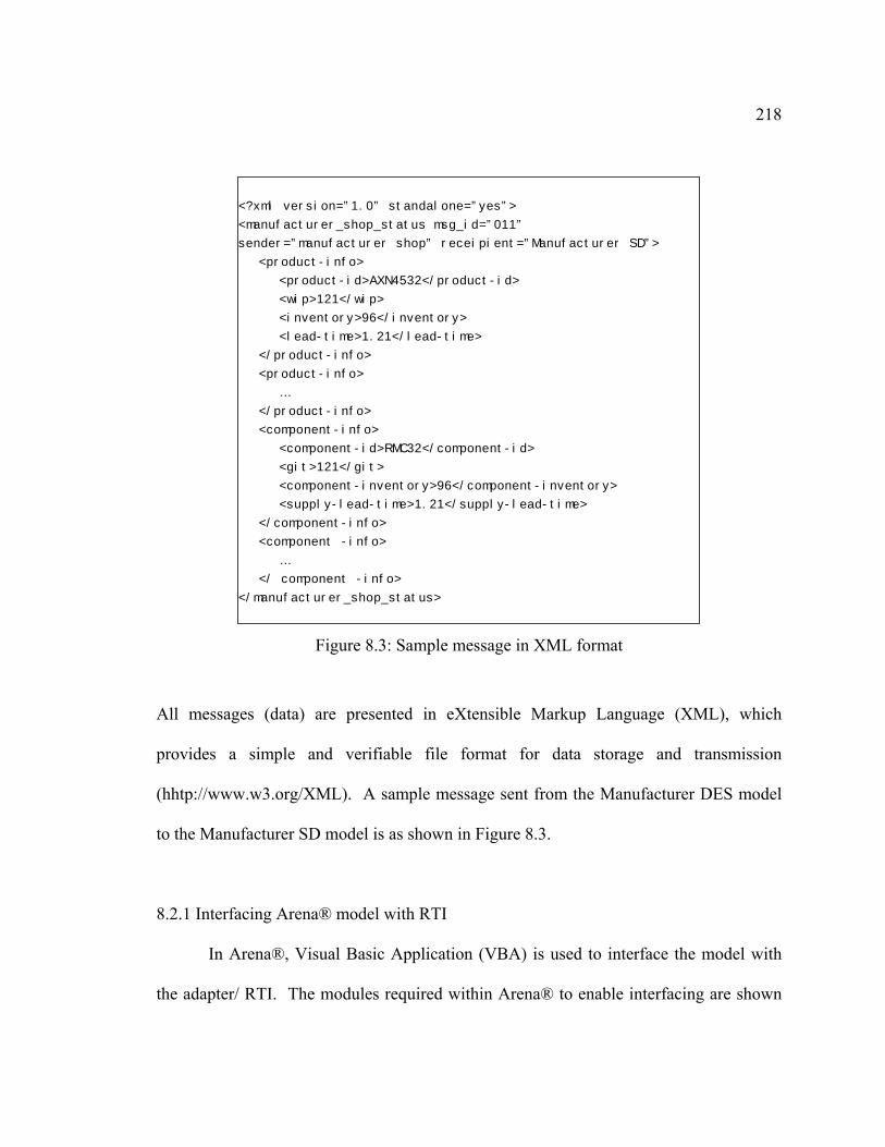
218

<?xml version=”1.0” standalone=”yes”>

<manufacturer_shop_status msg_id=”011”

sender=”manufacturer shop” receipient=”Manufacturer SD”>

<product-info>

<product-id>AXN4532</product-id>

<wip>121</wip>

<inventory>96</inventory>

<lead-time>1.21</lead-time>

</product-info>

<product-info>

…

</product-info>

<component-info>

<component-id>RMC32</component-id>

<git>121</git>

<component-inventory>96</component-inventory>

<supply-lead-time>1.21</supply-lead-time>

</component-info>

<component -info>

…

</ component -info>

</manufacturer_shop_status>

Figure 8.3: Sample message in XML format

All messages (data) are presented in eXtensible Markup Language (XML), which

provides a simple and verifiable file format for data storage and transmission

(hhtp://www.w3.org/XML). A sample message sent from the Manufacturer DES model

to the Manufacturer SD model is as shown in Figure 8.3.

8.2.1 Interfacing Arena® model with RTI

In Arena®, Visual Basic Application (VBA) is used to interface the model with

the adapter/ RTI. The modules required within Arena® to enable interfacing are shown

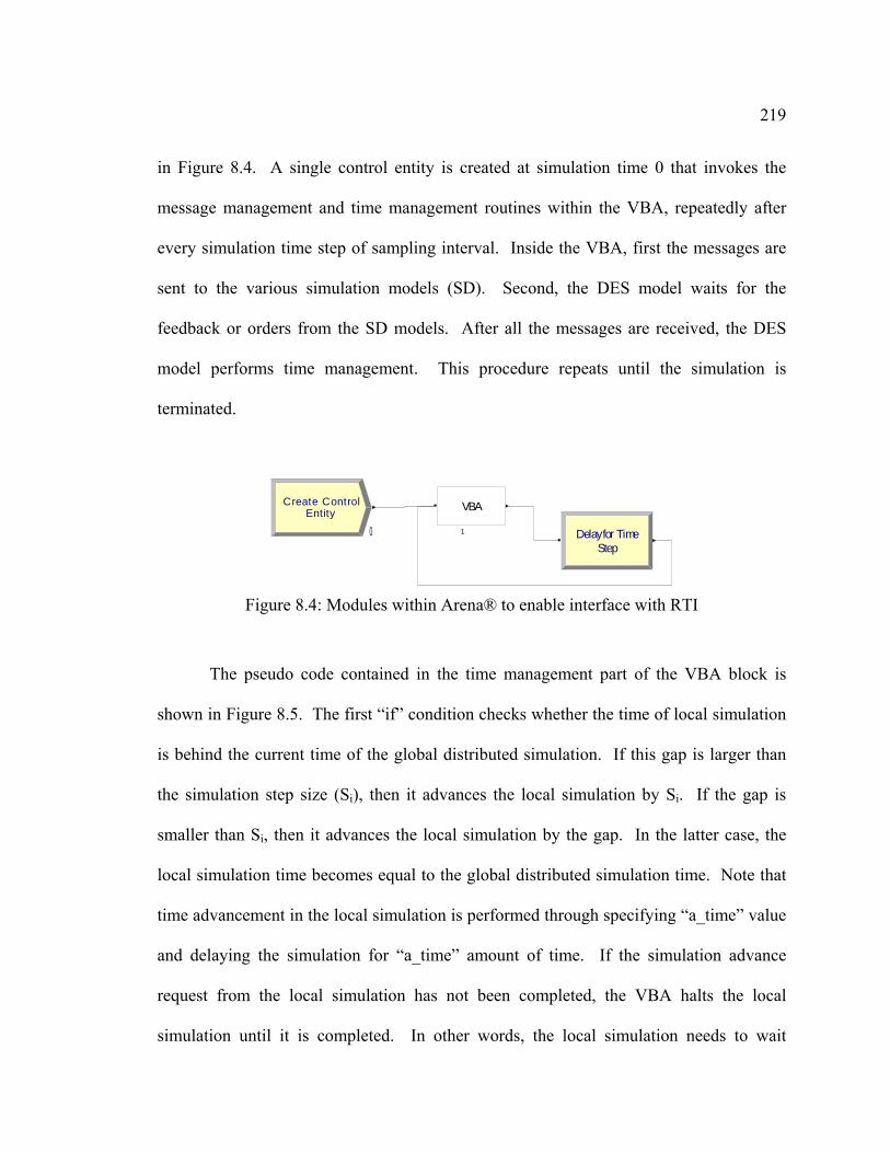
219

in Figure 8.4. A single control entity is created at simulation time 0 that invokes the

message management and time management routines within the VBA, repeatedly after

every simulation time step of sampling interval. Inside the VBA, first the messages are

sent to the various simulation models (SD). Second, the DES model waits for the

feedback or orders from the SD models. After all the messages are received, the DES

model performs time management. This procedure repeats until the simulation is

terminated.

EntityCreate Control

1

VBA

StepDelay for Time0

Figure 8.4: Modules within Arena® to enable interface with RTI

The pseudo code contained in the time management part of the VBA block is

shown in Figure 8.5. The first “if” condition checks whether the time of local simulation

is behind the current time of the global distributed simulation. If this gap is larger than

the simulation step size (Si), then it advances the local simulation by Si. If the gap is

smaller than Si, then it advances the local simulation by the gap. In the latter case, the

local simulation time becomes equal to the global distributed simulation time. Note that

time advancement in the local simulation is performed through specifying “a_time” value

and delaying the simulation for “a_time” amount of time. If the simulation advance

request from the local simulation has not been completed, the VBA halts the local

simulation until it is completed. In other words, the local simulation needs to wait

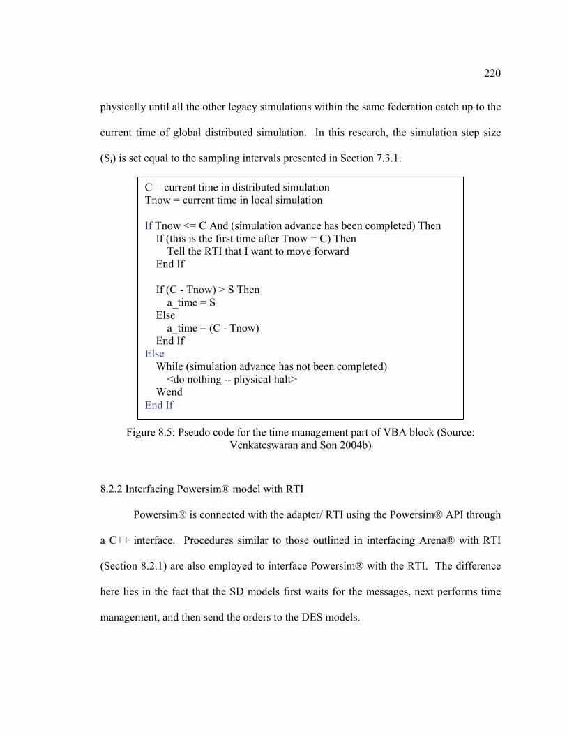
220

physically until all the other legacy simulations within the same federation catch up to the

current time of global distributed simulation. In this research, the simulation step size

(Si) is set equal to the sampling intervals presented in Section 7.3.1.

C = current time in distributed simulation Tnow = current time in local simulation If Tnow <= C And (simulation advance has been completed) Then If (this is the first time after Tnow = C) Then Tell the RTI that I want to move forward End If If (C - Tnow) > S Then a_time = S Else a_time = (C - Tnow) End If Else While (simulation advance has not been completed) <do nothing -- physical halt> Wend End If

Figure 8.5: Pseudo code for the time management part of VBA block (Source:

Venkateswaran and Son 2004b)

8.2.2 Interfacing Powersim® model with RTI

Powersim® is connected with the adapter/ RTI using the Powersim® API through

a C++ interface. Procedures similar to those outlined in interfacing Arena® with RTI

(Section 8.2.1) are also employed to interface Powersim® with the RTI. The difference

here lies in the fact that the SD models first waits for the messages, next performs time

management, and then send the orders to the DES models.

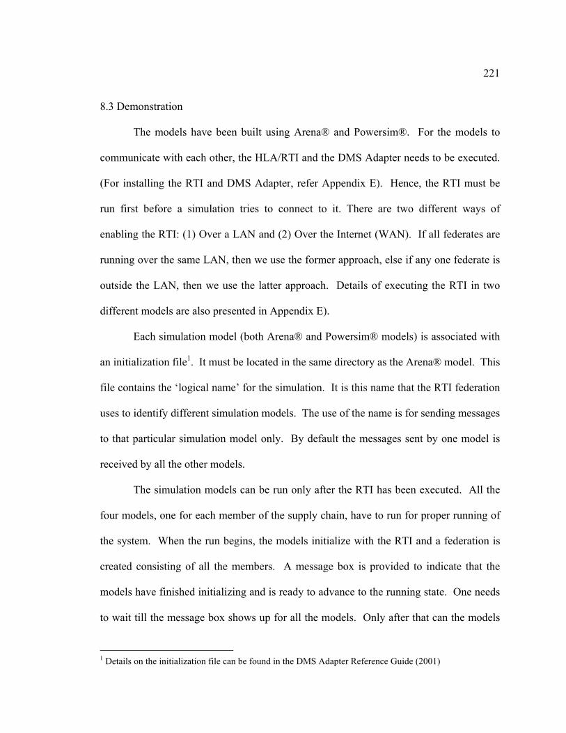
221

8.3 Demonstration

The models have been built using Arena® and Powersim®. For the models to

communicate with each other, the HLA/RTI and the DMS Adapter needs to be executed.

(For installing the RTI and DMS Adapter, refer Appendix E). Hence, the RTI must be

run first before a simulation tries to connect to it. There are two different ways of

enabling the RTI: (1) Over a LAN and (2) Over the Internet (WAN). If all federates are

running over the same LAN, then we use the former approach, else if any one federate is

outside the LAN, then we use the latter approach. Details of executing the RTI in two

different models are also presented in Appendix E).

Each simulation model (both Arena® and Powersim® models) is associated with

an initialization file1. It must be located in the same directory as the Arena® model. This

file contains the ‘logical name’ for the simulation. It is this name that the RTI federation

uses to identify different simulation models. The use of the name is for sending messages

to that particular simulation model only. By default the messages sent by one model is

received by all the other models.

The simulation models can be run only after the RTI has been executed. All the

four models, one for each member of the supply chain, have to run for proper running of

the system. When the run begins, the models initialize with the RTI and a federation is

created consisting of all the members. A message box is provided to indicate that the

models have finished initializing and is ready to advance to the running state. One needs

to wait till the message box shows up for all the models. Only after that can the models

1 Details on the initialization file can be found in the DMS Adapter Reference Guide (2001)

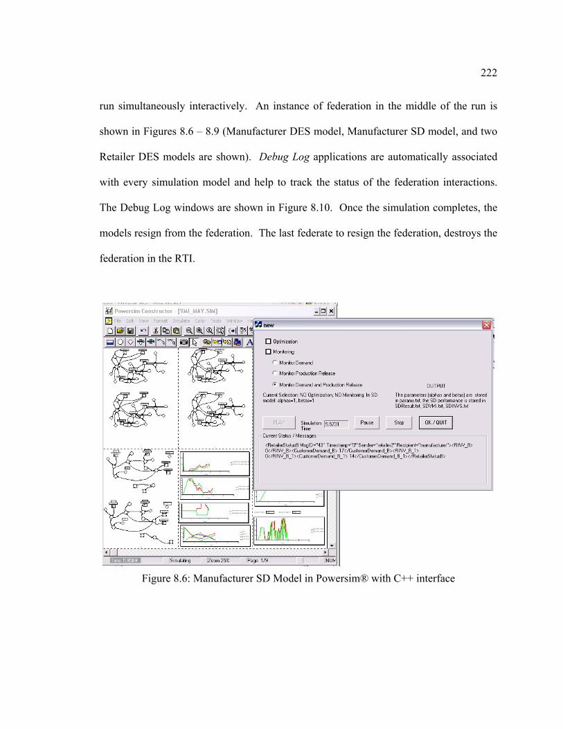
222

run simultaneously interactively. An instance of federation in the middle of the run is

shown in Figures 8.6 – 8.9 (Manufacturer DES model, Manufacturer SD model, and two

Retailer DES models are shown). Debug Log applications are automatically associated

with every simulation model and help to track the status of the federation interactions.

The Debug Log windows are shown in Figure 8.10. Once the simulation completes, the

models resign from the federation. The last federate to resign the federation, destroys the

federation in the RTI.

Figure 8.6: Manufacturer SD Model in Powersim® with C++ interface

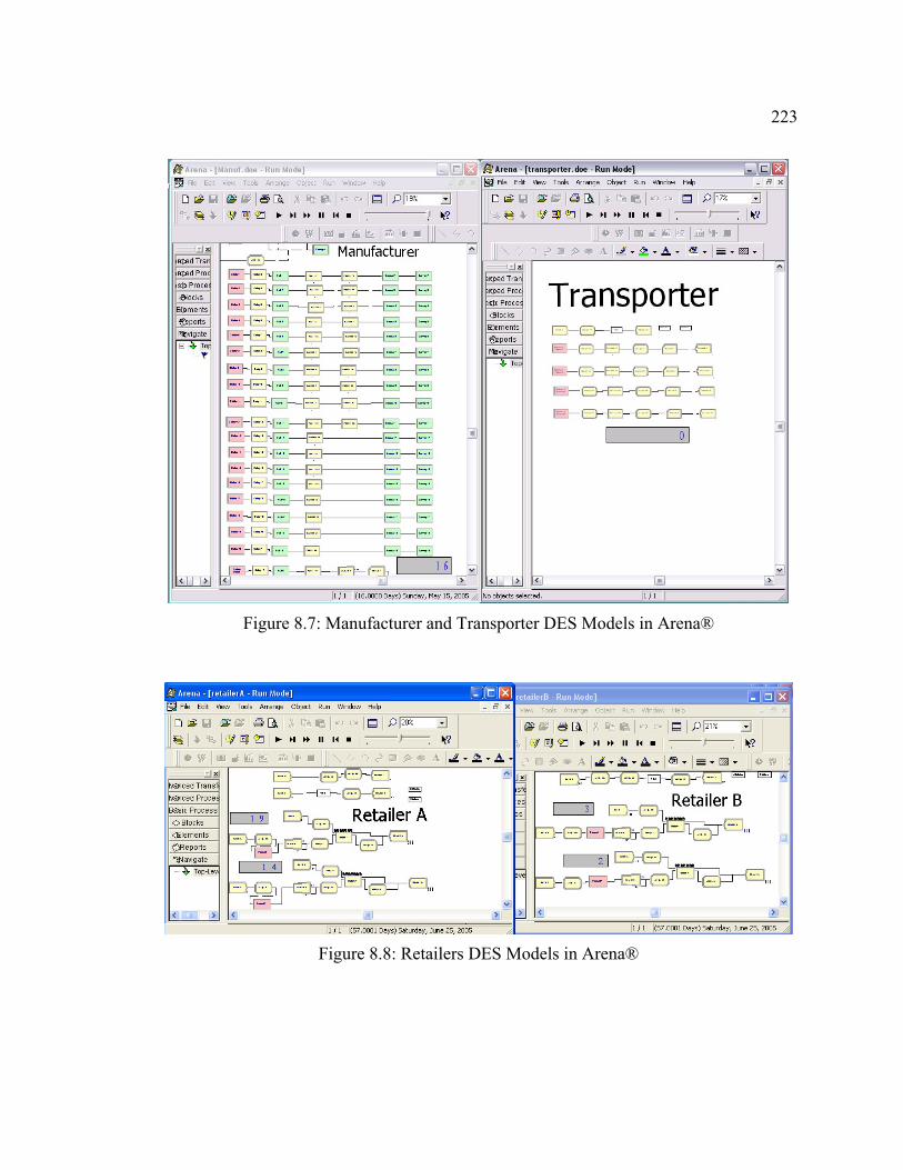
223

Figure 8.7: Manufacturer and Transporter DES Models in Arena®

Figure 8.8: Retailers DES Models in Arena®

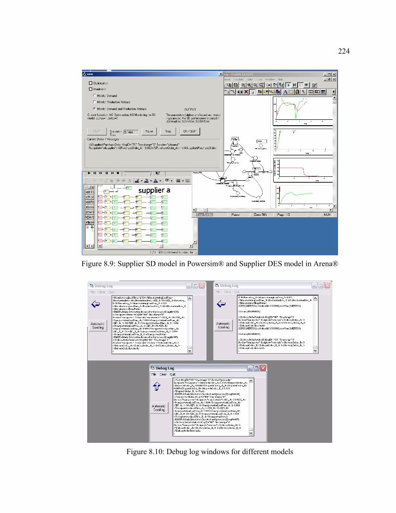
224

Figure 8.9: Supplier SD model in Powersim® and Supplier DES model in Arena®

Figure 8.10: Debug log windows for different models

225

CHAPTER 9

EXPERIMENTATION AND RESULTS

The purpose of the experiments is to demonstrate the proposed hybrid simulation-

based architecture for the analysis of supply chains. It is recalled that in supply chain

scenario considered, there exists two configurations. The communicative supply chain

configuration consists of two Suppliers, Transporter and the Manufacturer. The

Manufacturer orders component 1 with Supplier A and component 2 with Supplier B.

Both components are required for the production of products 1 and 2 at the Manufacturer.

Next, under collaborative configuration, the supply chain consists of Retailers,

Transporter and the Manufacturer, who manages the inventory at the Retailers through

the use of VMI. Products 1 and 2 are in demand at all the Retailers. The experiments are

been broken down into two parts: the communicative configuration supply chain and

collaborative configuration supply chain. It is noted that the Stage I activities have

already been performed for the supply chain scenario (refer Section 5.7). Hence, Stages

II-IV activities are discussed in this chapter.

In the communicative configuration supply chain, the functioning of the proposed

architecture is illustrated using exemplary sales patterns. First, the results of Stage II

optimization at the Manufacturer and Suppliers are presented. Next, the results of Stage

IV evaluation of the optimal control parameters determined from Stage II are analyzed to

better understand the global consequence of the local plans determined at each supply

chain member.

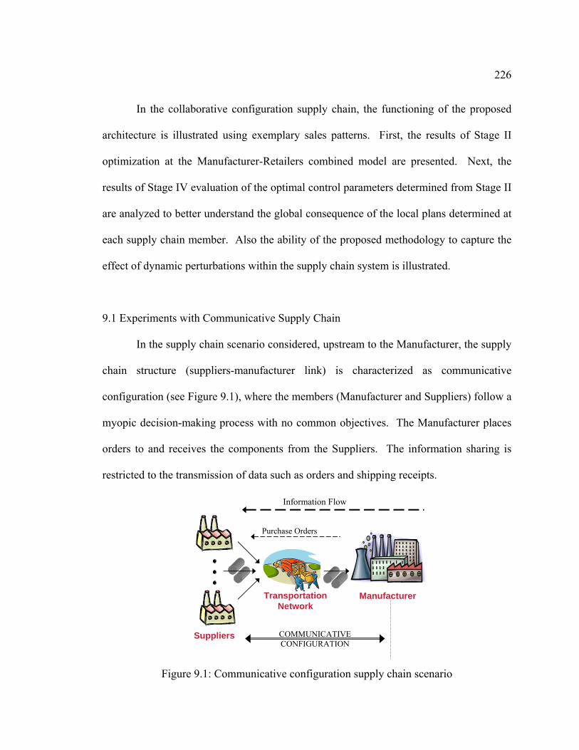
226

In the collaborative configuration supply chain, the functioning of the proposed

architecture is illustrated using exemplary sales patterns. First, the results of Stage II

optimization at the Manufacturer-Retailers combined model are presented. Next, the

results of Stage IV evaluation of the optimal control parameters determined from Stage II

are analyzed to better understand the global consequence of the local plans determined at

each supply chain member. Also the ability of the proposed methodology to capture the

effect of dynamic perturbations within the supply chain system is illustrated.

9.1 Experiments with Communicative Supply Chain

In the supply chain scenario considered, upstream to the Manufacturer, the supply

chain structure (suppliers-manufacturer link) is characterized as communicative

configuration (see Figure 9.1), where the members (Manufacturer and Suppliers) follow a

myopic decision-making process with no common objectives. The Manufacturer places

orders to and receives the components from the Suppliers. The information sharing is

restricted to the transmission of data such as orders and shipping receipts.

Suppliers

Manufacturer TransportationNetwork

Information Flow


Purchase Orders

Figure 9.1: Communicative configuration supply chain scenario

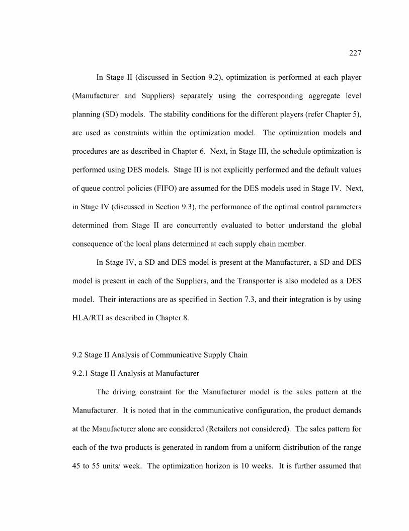
227

In Stage II (discussed in Section 9.2), optimization is performed at each player

(Manufacturer and Suppliers) separately using the corresponding aggregate level

planning (SD) models. The stability conditions for the different players (refer Chapter 5),

are used as constraints within the optimization model. The optimization models and

procedures are as described in Chapter 6. Next, in Stage III, the schedule optimization is

performed using DES models. Stage III is not explicitly performed and the default values

of queue control policies (FIFO) are assumed for the DES models used in Stage IV. Next,

in Stage IV (discussed in Section 9.3), the performance of the optimal control parameters

determined from Stage II are concurrently evaluated to better understand the global

consequence of the local plans determined at each supply chain member.

In Stage IV, a SD and DES model is present at the Manufacturer, a SD and DES

model is present in each of the Suppliers, and the Transporter is also modeled as a DES

model. Their interactions are as specified in Section 7.3, and their integration is by using

HLA/RTI as described in Chapter 8.

9.2 Stage II Analysis of Communicative Supply Chain

9.2.1 Stage II Analysis at Manufacturer

The driving constraint for the Manufacturer model is the sales pattern at the

Manufacturer. It is noted that in the communicative configuration, the product demands

at the Manufacturer alone are considered (Retailers not considered). The sales pattern for

each of the two products is generated in random from a uniform distribution of the range

45 to 55 units/ week. The optimization horizon is 10 weeks. It is further assumed that

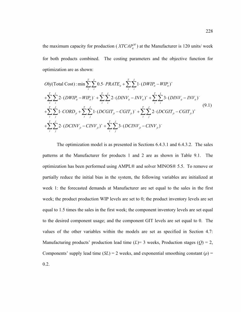
228

the maximum capacity for production ( MqXTCAP ) at the Manufacturer is 120 units/ week

for both products combined. The costing parameters and the objective function for

optimization are as shown:

(9.1)

(Total Cost) : min 0.5 1 ( )

2 ( ) 2 ( ) 3 ( )

1 1 ( ) 2 (

T I T I

it it itt i t i

T I T I T I

it it it it it itt i t i t i

T J T J T J

jt jt jt jt jtt j t j t j

Obj PRATE DWIP WIP

DWIP WIP DINV INV DINV INV

CORD DCGIT CGIT DCGIT CGIT

+

− +

− +

⋅ + ⋅ −

+ ⋅ − + ⋅ − + ⋅ −

+ ⋅ + ⋅ − + ⋅ −

+

∑∑ ∑∑

∑∑ ∑∑ ∑∑

∑∑ ∑∑ ∑∑

2 ( ) 3 ( )T J T J

jt jt jt jtt j t j

DCINV CINV DCINV CINV+ −⋅ − + ⋅ −∑∑ ∑∑

)

−

The optimization model is as presented in Sections 6.4.3.1 and 6.4.3.2. The sales

patterns at the Manufacturer for products 1 and 2 are as shown in Table 9.1. The

optimization has been performed using AMPL® and solver MINOS® 5.5. To remove or

partially reduce the initial bias in the system, the following variables are initialized at

week 1: the forecasted demands at Manufacturer are set equal to the sales in the first

week; the product production WIP levels are set to 0; the product inventory levels are set

equal to 1.5 times the sales in the first week; the component inventory levels are set equal

to the desired component usage; and the component GIT levels are set equal to 0. The

values of the other variables within the models are set as specified in Section 4.7:

Manufacturing products’ production lead time (L)= 3 weeks, Production stages (Q) = 2,

Components’ supply lead time (SL) = 2 weeks, and exponential smoothing constant (ρ) =

0.2.

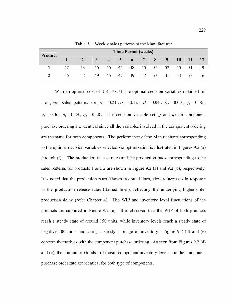
229

Table 9.1: Weekly sales patterns at the Manufacturer

Time Period (weeks) Product

1 2 3 4 5 6 7 8 9 10 11 12

1 52 53 46 46 45 48 45 55 52 45 51 49

2 55 52 49 45 47 49 52 53 45 54 53 46

With an optimal cost of $14,178.71, the optimal decision variables obtained for

the given sales patterns are: 1 0.21α = , 2 0.12α = , 1 0.04β = , 2 0.00β = , 1 0.36γ = ,

2 0.36γ = , 1 0.28η = , 2 0.28η = . The decision variable set (γ and η) for component

purchase ordering are identical since all the variables involved in the component ordering

are the same for both components. The performance of the Manufacturer corresponding

to the optimal decision variables selected via optimization is illustrated in Figures 9.2 (a)

through (f). The production release rates and the production rates corresponding to the

sales patterns for products 1 and 2 are shown in Figure 9.2 (a) and 9.2 (b), respectively.

It is noted that the production rates (shown in dotted lines) slowly increases in response

to the production release rates (dashed lines), reflecting the underlying higher-order

production delay (refer Chapter 4). The WIP and inventory level fluctuations of the

products are captured in Figure 9.2 (c). It is observed that the WIP of both products

reach a steady state of around 150 units, while inventory levels reach a steady state of

negative 100 units, indicating a steady shortage of inventory. Figure 9.2 (d) and (e)

concern themselves with the component purchase ordering. As seen from Figures 9.2 (d)

and (e), the amount of Goods-in-Transit, component inventory levels and the component

purchase order rate are identical for both type of components.

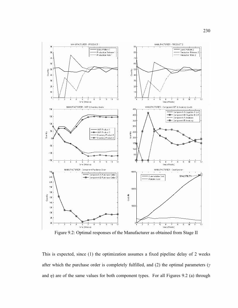
230

Figure 9.2: Optimal responses of the Manufacturer as obtained from Stage II

This is expected, since (1) the optimization assumes a fixed pipeline delay of 2 weeks

after which the purchase order is completely fulfilled, and (2) the optimal parameters (γ

and η) are of the same values for both component types. For all Figures 9.2 (a) through

231

(e), it is observed that the values of each variable reach the corresponding steady state

after week 7. In steady state, it is seen the fundamental laws such as Little’s laws are

satisfied, thus providing a validation for the models developed. For example, the product

production rates reach an approximate steady of 50 units/ week in response to sales

around 50 units/ week. Given a 3-week lead time for production, this (Little’s Law)

would require that the WIP levels to reach (50 x 3 = 150 units). This is observed in

Figure 9.2 (c). Finally, Figure 9.2 (f) plots the progression of the system cost objective

function (Equation 9.1) over time. The total optimal cost for the entire time period is

found to be optimal cost of $14,178.71.

9.2.2 Stage II Analysis at Suppliers

Two suppliers are considered in the supply chain. The driving constraint (sales

pattern) for both the suppliers is taken as the corresponding component purchase plan

obtained at the Manufacturer (see Figure 9.2 e). Each supplier is optimized for 10 weeks.

The optimization models are as presented in Section 6.4.1 and 6.4.2. The costing

parameters and the objective function for optimization for both suppliers is as follows:

(Total Cost) : min 1

2 [ ] 3 [ ]

2 [ ] 3 [ ]

T

jtt

T T

jt jt jt jtt t

T T

jt jt jt jtt t

SupplierObj SPRATE

SDWIP SWIP SDWIP SWIP

SDINV SINV SDINV SINV

+ +

+ −

⋅

+ ⋅ − + ⋅ −

+ ⋅ − + ⋅ −

∑

∑ ∑

∑ ∑

To remove or reduce the initial bias in the system, the following variables are initialized

at week 1: the forecasted demands at Suppliers are set equal to the sales in the first week;

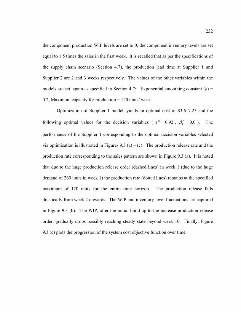
232

the component production WIP levels are set to 0; the component inventory levels are set

equal to 1.5 times the sales in the first week. It is recalled that as per the specifications of

the supply chain scenario (Section 4.7), the production lead time at Supplier 1 and

Supplier 2 are 2 and 3 weeks respectively. The values of the other variables within the

models are set, again as specified in Section 4.7: Exponential smoothing constant (ρ) =

0.2, Maximum capacity for production = 120 units/ week.

Optimization of Supplier 1 model, yields an optimal cost of $3,617.23 and the

following optimal values for the decision variables ( , ). The

performance of the Supplier 1 corresponding to the optimal decision variables selected

via optimization is illustrated in Figures 9.3 (a) – (c). The production release rate and the

production rate corresponding to the sales pattern are shown in Figure 9.3 (a). It is noted

that due to the huge production release order (dashed lines) in week 1 (due to the huge

demand of 260 units in week 1) the production rate (dotted lines) remains at the specified

maximum of 120 units for the entire time horizon. The production release falls

drastically from week 2 onwards. The WIP and inventory level fluctuations are captured

in Figure 9.3 (b). The WIP, after the initial build-up to the increase production release

order, gradually drops possibly reaching steady state beyond week 10. Finally, Figure

9.3 (c) plots the progression of the system cost objective function over time.

1 0.92Rα = 1 0.0Rβ =

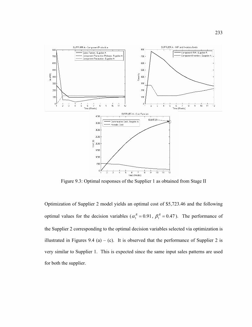
233

Figure 9.3: Optimal responses of the Supplier 1 as obtained from Stage II

Optimization of Supplier 2 model yields an optimal cost of $5,723.46 and the following

optimal values for the decision variables ( , ). The performance of

the Supplier 2 corresponding to the optimal decision variables selected via optimization is

illustrated in Figures 9.4 (a) – (c). It is observed that the performance of Supplier 2 is

very similar to Supplier 1. This is expected since the same input sales patterns are used

for both the supplier.

1 0.91Rα = 1 0.47Rβ =

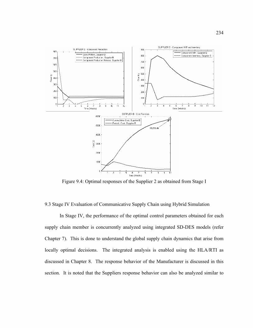
234

Figure 9.4: Optimal responses of the Supplier 2 as obtained from Stage I

9.3 Stage IV Evaluation of Communicative Supply Chain using Hybrid Simulation

In Stage IV, the performance of the optimal control parameters obtained for each

supply chain member is concurrently analyzed using integrated SD-DES models (refer

Chapter 7). This is done to understand the global supply chain dynamics that arise from

locally optimal decisions. The integrated analysis is enabled using the HLA/RTI as

discussed in Chapter 8. The response behavior of the Manufacturer is discussed in this

section. It is noted that the Suppliers response behavior can also be analyzed similar to

235

the Manufacturer. However, since the necessary insights are obtained using the response

of the Manufacturer, those are alone discussed.

Two experiments are conducted based on the settings of the sampling intervals

between the supply chain members. It is recalled that sampling interval for Manufacturer

and Supplier 2 is fixed at 1 day (1/7 week), while the sampling interval for Supplier 1 is

fixed at 1 week (refer Section 5.7). The sampling interval corresponds to the frequency

of information update within each member. An interval of 1 day means that the member

gathers the data and makes decisions (regarding production, purchase and shipment)

every day. An interval of 1 week means that the member gathers data and makes

decisions only every week. Hence, Supplier 1 releases a production order at the

beginning of each week; dispatched parts for shipment at the beginning of each week;

and receives purchase order from the Manufacturer the beginning of each week.

First, in Section 9.3.1, the experimental results from the supply chain operating

with the same sampling intervals across members (1 day sampling interval is assumed for

Supplier 1) is discussed. Next, in Section 9.3.2, the experimental results from the supply

chain operating with the different sampling intervals across members (1 week sampling

interval is assumed for Supplier 1) is discussed.

9.3.1 Stage IV Analysis: Same Sampling Interval among Supply Chain Members

The experimental results from the supply chain operating with the same sampling

intervals across members (1 day sampling interval is assumed for Supplier 1) are

presented. The sampling interval between the intra-member models (SD and DES

236

models of the each member) is 1 day, and the inter-member models (SD and DES models

of one member interacting with the other members’ models) is also 1 day. The SD

model converts the weekly rates into daily rates and sends them to the DES models. The

DES models simulate the detailed operations for a time period of 1 day, and update the

current operational status in the SD models. The response behavior of the Manufacturer,

as obtained by integrated analysis in Stage IV, is shown in Figure 9.5 (a) – (f). The

production release rates and the production rates for products 1 and 2 are as shown in

Figures 9.5 (a) and (b), respectively. Though there are increased fluctuations in the rates,

it is seen that the fluctuations are damped with decreasing amplitudes. Also, the trend in

the rates is comparable with those in Figures 9.2 (a) and (b). The levels of WIP for both

products overlap, and inventory levels for both products overlap (Figure 9.5 c). The WIP

flattens out (steady state) at about 100 units, as opposed to 150 units suggested by Stage

II (Figure 9.2 c). The increased WIP levels in the aggregate model (Stage II) can be

attributed to the way in which the production process is aggregated, and indicates that the

production lead time and the higher-order delays (refer Chapter 4) needs to be fine tuned.

Figure 9.5 (d) shows the component GIT and component inventory levels at the

Manufacturer. In Stage II (Figure 9.2 d) the GIT levels of the component tapers down to

around 200 units, a reflection of the supply lead time of 2 weeks. In Stage IV (Figure 9.5

d) the GIT levels increases to and hovers around 400 units. This is attributed to the

inclusion of the time component purchase orders stay in the backlog of the Suppliers.

These cannot be captured within the Manufacturer model in Stage II without extensive

interaction with the Suppliers and the nature of transportation network employed, which

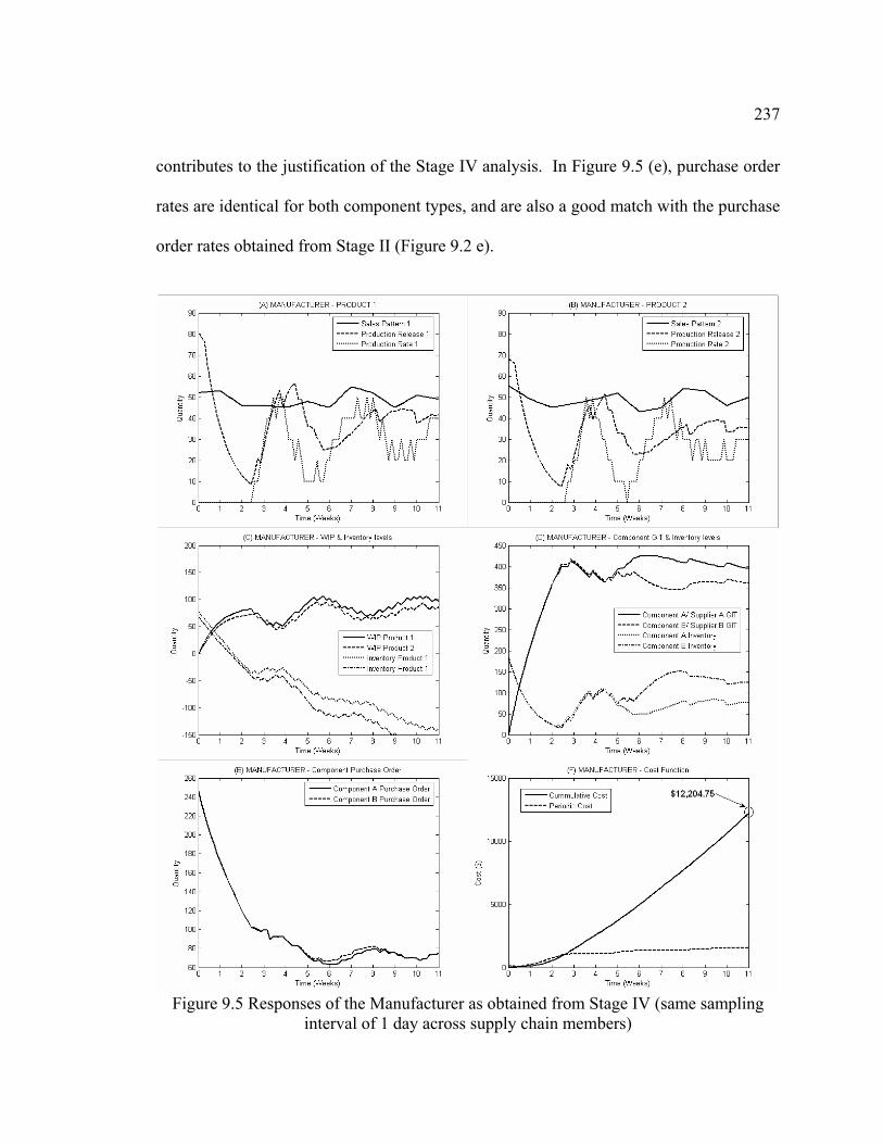
237

contributes to the justification of the Stage IV analysis. In Figure 9.5 (e), purchase order

rates are identical for both component types, and are also a good match with the purchase

order rates obtained from Stage II (Figure 9.2 e).

Figure 9.5 Responses of the Manufacturer as obtained from Stage IV (same sampling

interval of 1 day across supply chain members)

238

The progression of the total cost objective function obtained from Stage IV analysis is

plotted in Figure 9.5 (f). The cumulative costs ($12,204.75) in Stage IV are slightly

lower the costs ($14,178.91) in Stage II. This indicates that, (1) the optimal plan is

feasible in the actual supply chain, and (2) the models employed in Stage II are

pessimistic in its estimations.

9.3.2 Stage IV Analysis: Different Sampling Interval among Supply Chain Members

The experimental results from the supply chain operating with the different

sampling intervals across members (1 week sampling interval is assumed for Supplier 1)

are discussed in this section. The sampling interval between the intra-member models

(SD and DES models of each member) is 1 day for Manufacturer and Supplier 2. The

sampling interval between Manufacturer and Supplier 2 models are also 1 day. Now, the

sampling interval of intra-member models (SD and DES models) of the Supplier 1 is one

week. Also, the sampling interval between Manufacturer and Supplier 1 is one week.

The response behavior of the Manufacturer, as obtained by integrated analysis in Stage

IV, is shown in Figure 9.6 (a) – (f). The product production release rates and the

production rates (Figures 9.6 a, b) show a fluctuating trend similar to those in Figure 9.5

(a) and (b). Also, it is noted that the product production release is contingent upon the

availability of both the raw material components, and a lower values in Figure 9.6 (a)

could be the result of less components being available with the Manufacturer at the time

of decision making. Figure 9.6 (c) shows the fluctuations in the WIP and inventory

levels of the products.

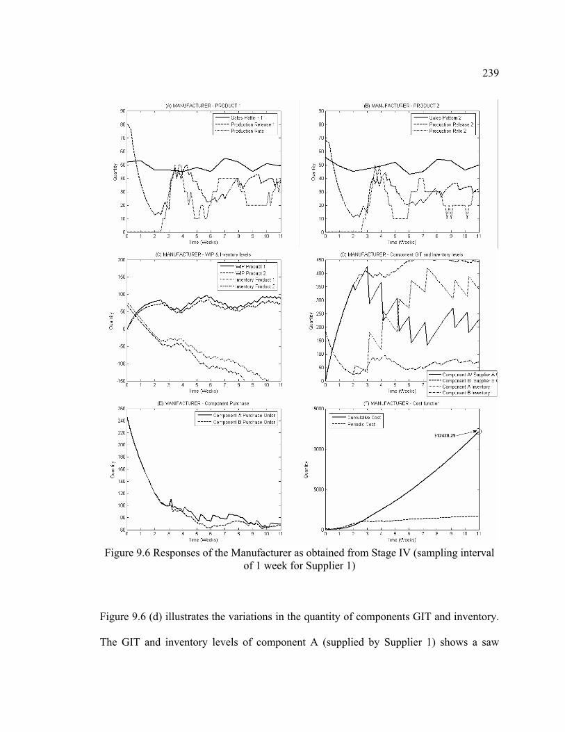
239

Figure 9.6 Responses of the Manufacturer as obtained from Stage IV (sampling interval

of 1 week for Supplier 1)

Figure 9.6 (d) illustrates the variations in the quantity of components GIT and inventory.

The GIT and inventory levels of component A (supplied by Supplier 1) shows a saw

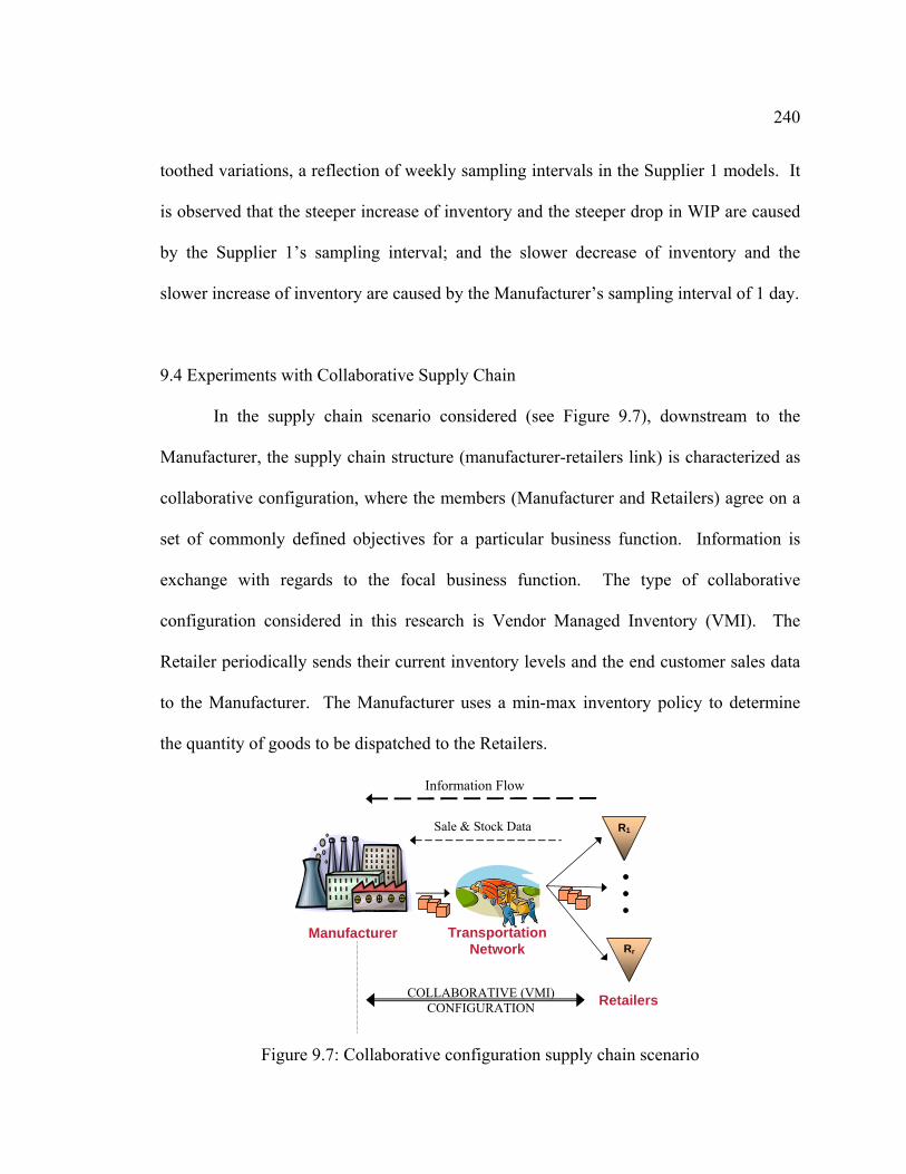
240

toothed variations, a reflection of weekly sampling intervals in the Supplier 1 models. It

is observed that the steeper increase of inventory and the steeper drop in WIP are caused

by the Supplier 1’s sampling interval; and the slower decrease of inventory and the

slower increase of inventory are caused by the Manufacturer’s sampling interval of 1 day.

9.4 Experiments with Collaborative Supply Chain

In the supply chain scenario considered (see Figure 9.7), downstream to the

Manufacturer, the supply chain structure (manufacturer-retailers link) is characterized as

collaborative configuration, where the members (Manufacturer and Retailers) agree on a

set of commonly defined objectives for a particular business function. Information is

exchange with regards to the focal business function. The type of collaborative

configuration considered in this research is Vendor Managed Inventory (VMI). The

Retailer periodically sends their current inventory levels and the end customer sales data

to the Manufacturer. The Manufacturer uses a min-max inventory policy to determine

the quantity of goods to be dispatched to the Retailers.

Manufacturer

Retailers

R1

Rr

Information Flow

Sale & Stock Data



Figure 9.7: Collaborative configuration supply chain scenario

241

In Stage II (discussed in Section 9.5), optimization is performed using the

combined Manufacturer-Retailer SD models. The stability conditions for the different

players (refer Chapter 5), are used as constraints within the optimization model. The

optimization models and procedures are as described in Chapter 6. Next, in Stage III, the

schedule optimization is performed using DES models. Stage III is not explicitly

performed and the default values of queue control policies (FIFO) are assumed for the

DES models used in Stage IV. Next, in Stage IV (discussed in Section 9.6), the

performance of the optimal control parameters determined from Stage II are evaluated to

better understand the global consequence of the local plans determined at each supply

chain member. In Stage IV, a SD and DES model is present at the Manufacturer, and

DES models are present at each of the Retailers, and the Transporter is also modeled as a

DES model. Their interactions are as specified in Section 7.3, and their integration is by

using HLA/RTI as described in Chapter 8.

9.5 Stage II Analysis of Collaborative Supply Chain

In Stage II, optimization of the aggregate level planning (SD) models is

performed. The driving constraint for the model is the end customer sales pattern at the

Retailers ( RiRSALES ). The demand pattern for each product at each Retailer is generated

in random from a uniform distribution of the range of 15 to 20 units/ week. The

optimization time horizon is 10 weeks. It is further assumed that the maximum capacity

for production ( MqXTCAP ) at the Manufacturer is 120 units/ week for both products

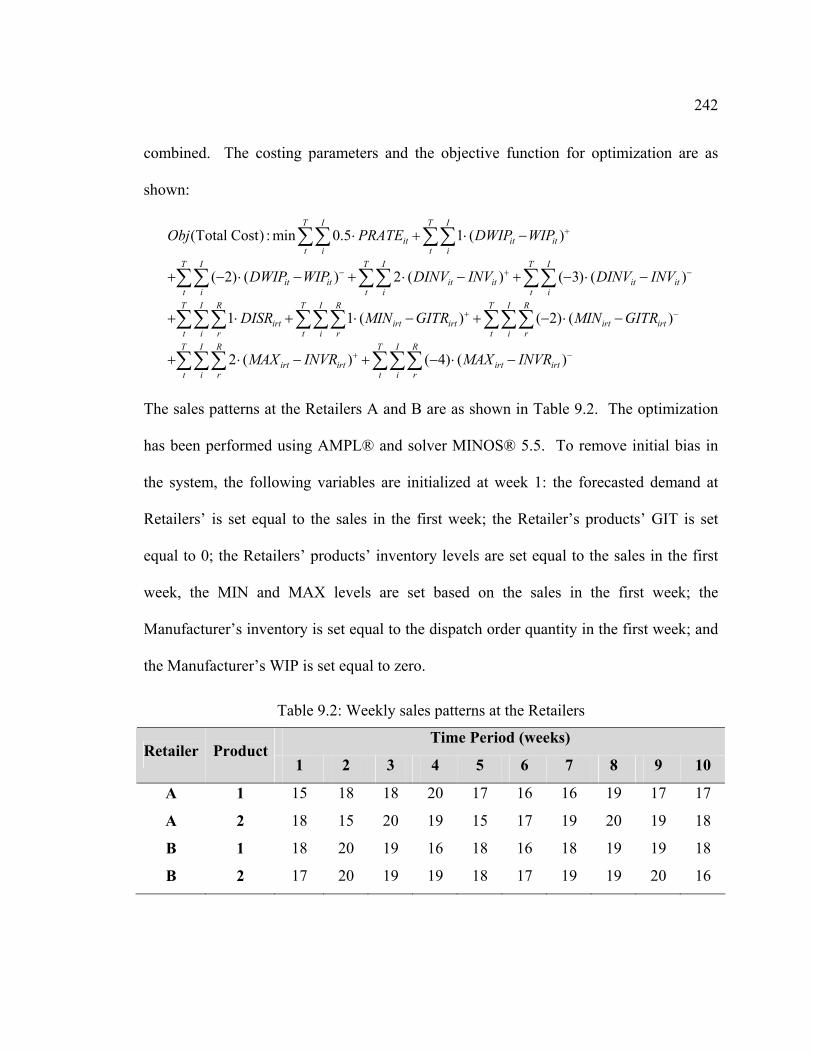
242

combined. The costing parameters and the objective function for optimization are as

shown:

(Total Cost) : min 0.5 1 ( )

( 2) ( ) 2 ( ) ( 3) ( )

1 1 ( ) ( 2) (

T I T I

it it itt i t i

T I T I T I

it it it it it itt i t i t iT I R T I R

irt irt irt irtt i r t i r

Obj PRATE DWIP WIP

DWIP WIP DINV INV DINV INV

DISR MIN GITR MIN

+

− + −

+

⋅ + ⋅ −

+ − ⋅ − + ⋅ − + − ⋅ −

+ ⋅ + ⋅ − + − ⋅ −

∑∑ ∑∑

∑∑ ∑∑ ∑∑

∑∑∑ ∑∑∑ )

2 ( ) ( 4) ( )

T I R

irtt i r

T I R T I R

irt irt irt irtt i r t i r

GITR

MAX INVR MAX INVR

−

+ −+ ⋅ − + − ⋅ −

∑∑∑

∑∑∑ ∑∑∑

The sales patterns at the Retailers A and B are as shown in Table 9.2. The optimization

has been performed using AMPL® and solver MINOS® 5.5. To remove initial bias in

the system, the following variables are initialized at week 1: the forecasted demand at

Retailers’ is set equal to the sales in the first week; the Retailer’s products’ GIT is set

equal to 0; the Retailers’ products’ inventory levels are set equal to the sales in the first

week, the MIN and MAX levels are set based on the sales in the first week; the

Manufacturer’s inventory is set equal to the dispatch order quantity in the first week; and

the Manufacturer’s WIP is set equal to zero.

Table 9.2: Weekly sales patterns at the Retailers

Time Period (weeks) Retailer Product

1 2 3 4 5 6 7 8 9 10

A 1 15 18 18 20 17 16 16 19 17 17

A 2 18 15 20 19 15 17 19 20 19 18

B 1 18 20 19 16 18 16 18 19 19 18

B 2 17 20 19 19 18 17 19 19 20 16

243

With the optimal cost of $7726.12, the optimal decision variables obtained for the

given sales patterns are as follows: 1 0.13α = , 2 0.0α = , 1 0.15β = , 2 0.10β = , 1 1.21Aψ = ,

2 1.32Aψ = , 1 1.29Bψ = , 2 1.3Bψ = , 1 0.91Aϕ = , 2 1.99Aϕ = , 1 1.74Bϕ = , and 2 2.01Bϕ = .

The performance of the supply chain corresponding to the optimal decision variables

selected via optimization in Stage II is as shown in Figure 9.8 (a) – (f). The production

release rates and the production rates at the Manufacturer’s are illustrated in Figure 9.8

(a). It is noted that the production rates (dotted lines) slowly increases in response to the

production release rates (solid lines), reflecting the underlying higher-order production

delay (refer Chapter 4). The product inventory levels fluctuations at the Manufacturer is

captured in Figure 9.8 (b). Figure 9.8 (c)-(f) plots the dynamics in the downstream

inventory (good-in-transit + Retailer inventory) as a thick solid line. The almost

horizontal lines in the graphs represent the MIN level (dashed line) and the MAX level

(solid thin line). For Retailer A (product 1), the goods are dispatched in weeks 1, 4 and 7

resulting in a marked increase in the downstream inventory in weeks 2, 5 and 8. Similarly,

Retailer A, product 2 is dispatched twice; for Retailer B, product 1 and 2 are dispatched

twice in the 10 week horizon.

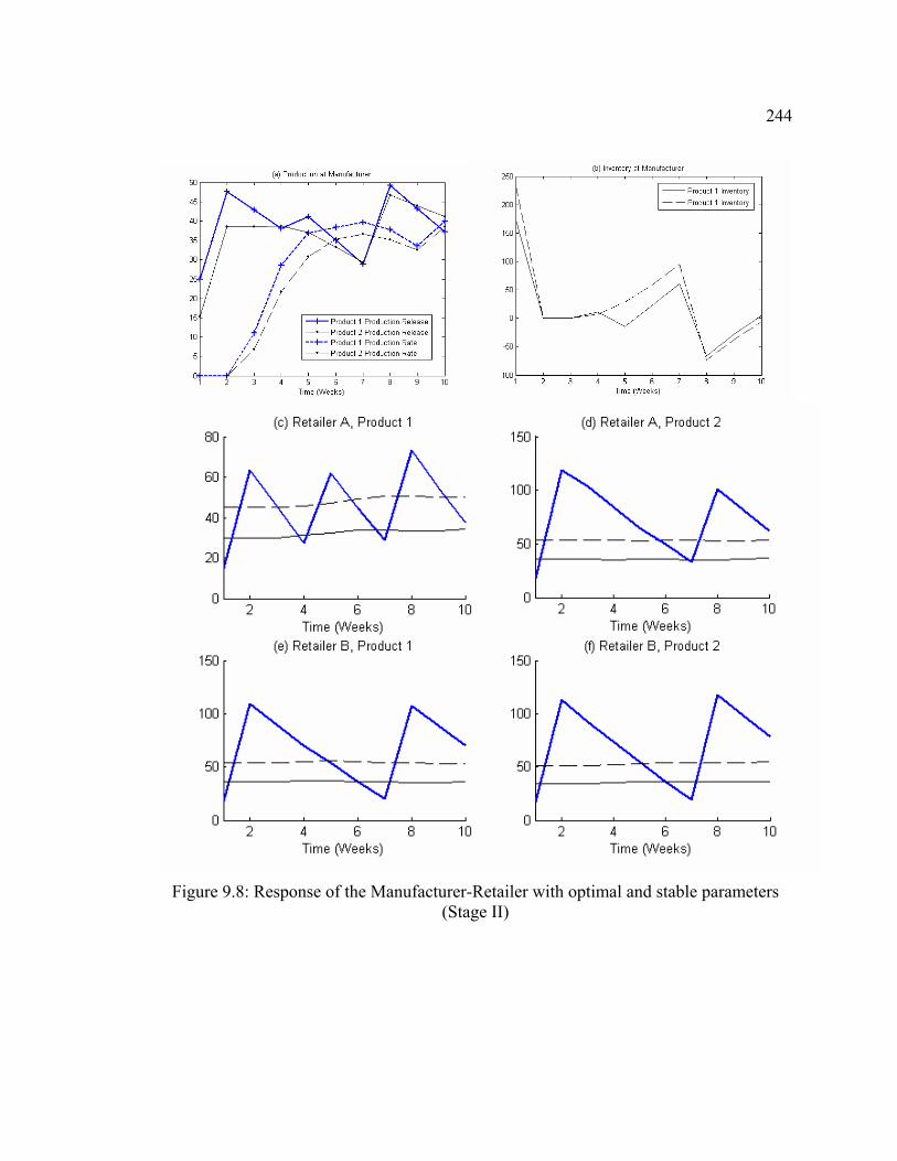
244

Figure 9.8: Response of the Manufacturer-Retailer with optimal and stable parameters

(Stage II)

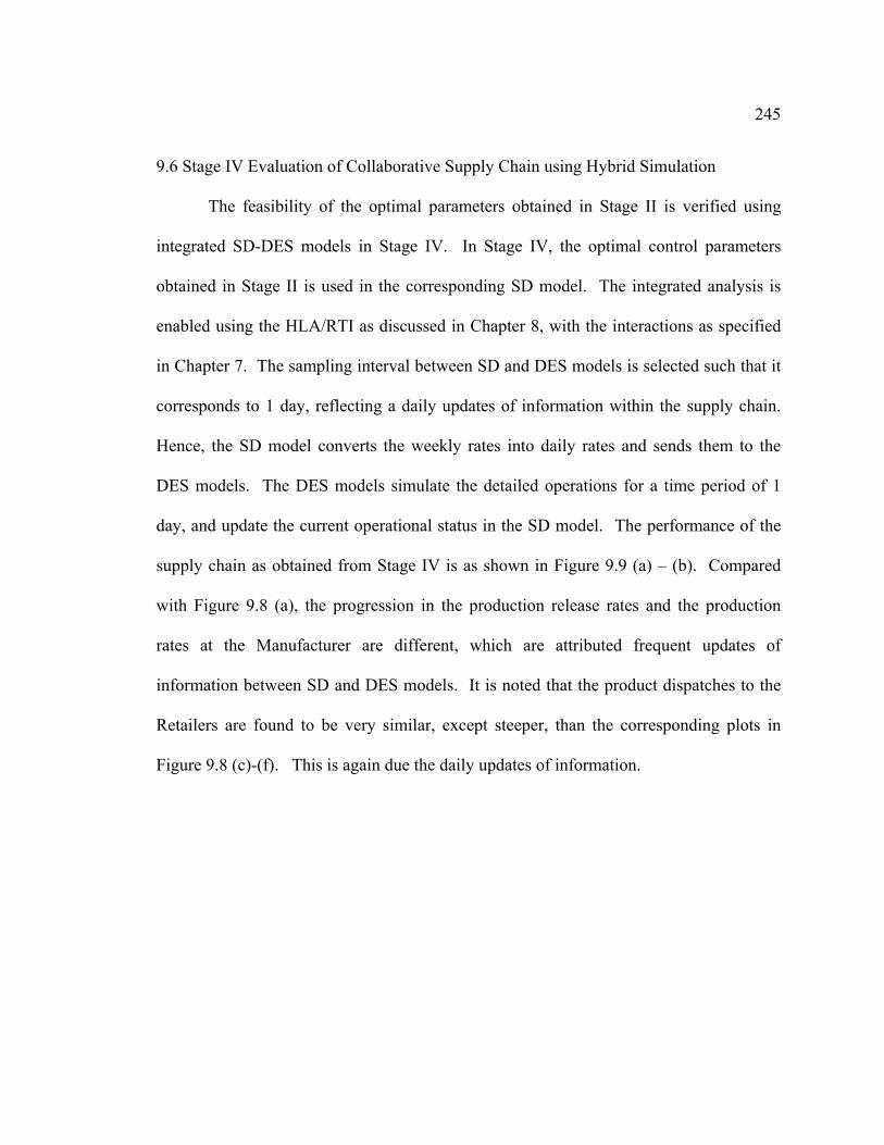
245

9.6 Stage IV Evaluation of Collaborative Supply Chain using Hybrid Simulation

The feasibility of the optimal parameters obtained in Stage II is verified using

integrated SD-DES models in Stage IV. In Stage IV, the optimal control parameters

obtained in Stage II is used in the corresponding SD model. The integrated analysis is

enabled using the HLA/RTI as discussed in Chapter 8, with the interactions as specified

in Chapter 7. The sampling interval between SD and DES models is selected such that it

corresponds to 1 day, reflecting a daily updates of information within the supply chain.

Hence, the SD model converts the weekly rates into daily rates and sends them to the

DES models. The DES models simulate the detailed operations for a time period of 1

day, and update the current operational status in the SD model. The performance of the

supply chain as obtained from Stage IV is as shown in Figure 9.9 (a) – (b). Compared

with Figure 9.8 (a), the progression in the production release rates and the production

rates at the Manufacturer are different, which are attributed frequent updates of

information between SD and DES models. It is noted that the product dispatches to the

Retailers are found to be very similar, except steeper, than the corresponding plots in

Figure 9.8 (c)-(f). This is again due the daily updates of information.

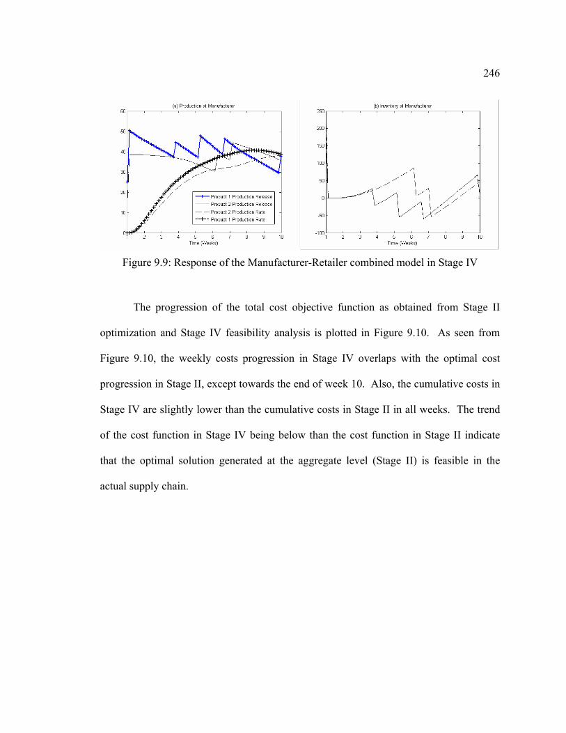
246

Figure 9.9: Response of the Manufacturer-Retailer combined model in Stage IV

The progression of the total cost objective function as obtained from Stage II

optimization and Stage IV feasibility analysis is plotted in Figure 9.10. As seen from

Figure 9.10, the weekly costs progression in Stage IV overlaps with the optimal cost

progression in Stage II, except towards the end of week 10. Also, the cumulative costs in

Stage IV are slightly lower than the cumulative costs in Stage II in all weeks. The trend

of the cost function in Stage IV being below than the cost function in Stage II indicate

that the optimal solution generated at the aggregate level (Stage II) is feasible in the

actual supply chain.

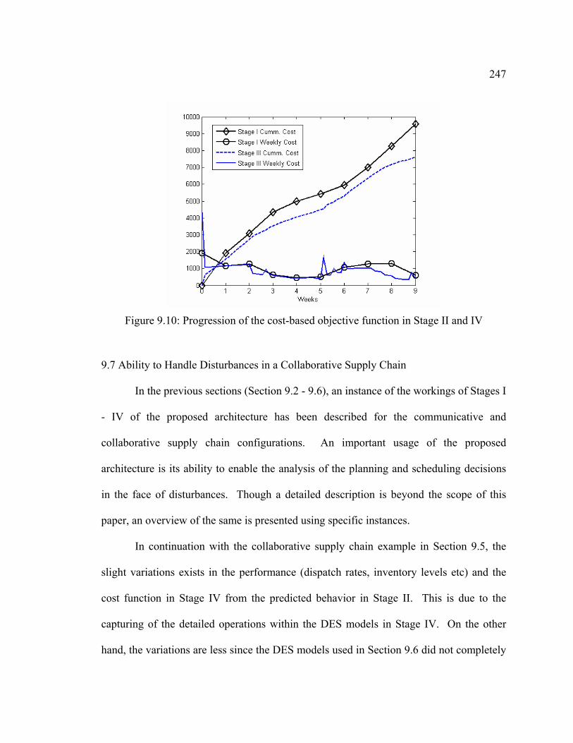
247

Figure 9.10: Progression of the cost-based objective function in Stage II and IV

9.7 Ability to Handle Disturbances in a Collaborative Supply Chain

In the previous sections (Section 9.2 - 9.6), an instance of the workings of Stages I

- IV of the proposed architecture has been described for the communicative and

collaborative supply chain configurations. An important usage of the proposed

architecture is its ability to enable the analysis of the planning and scheduling decisions

in the face of disturbances. Though a detailed description is beyond the scope of this

paper, an overview of the same is presented using specific instances.

In continuation with the collaborative supply chain example in Section 9.5, the

slight variations exists in the performance (dispatch rates, inventory levels etc) and the

cost function in Stage IV from the predicted behavior in Stage II. This is due to the

capturing of the detailed operations within the DES models in Stage IV. On the other

hand, the variations are less since the DES models used in Section 9.6 did not completely

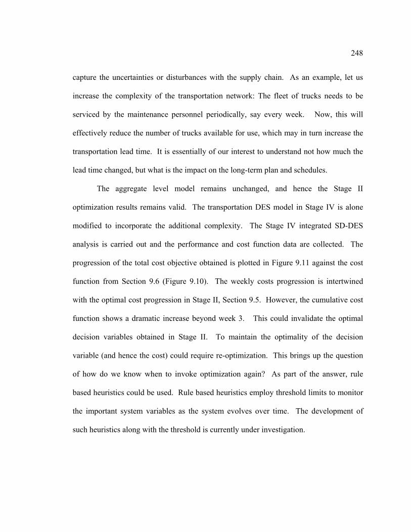
248

capture the uncertainties or disturbances with the supply chain. As an example, let us

increase the complexity of the transportation network: The fleet of trucks needs to be

serviced by the maintenance personnel periodically, say every week. Now, this will

effectively reduce the number of trucks available for use, which may in turn increase the

transportation lead time. It is essentially of our interest to understand not how much the

lead time changed, but what is the impact on the long-term plan and schedules.

The aggregate level model remains unchanged, and hence the Stage II

optimization results remains valid. The transportation DES model in Stage IV is alone

modified to incorporate the additional complexity. The Stage IV integrated SD-DES

analysis is carried out and the performance and cost function data are collected. The

progression of the total cost objective obtained is plotted in Figure 9.11 against the cost

function from Section 9.6 (Figure 9.10). The weekly costs progression is intertwined

with the optimal cost progression in Stage II, Section 9.5. However, the cumulative cost

function shows a dramatic increase beyond week 3. This could invalidate the optimal

decision variables obtained in Stage II. To maintain the optimality of the decision

variable (and hence the cost) could require re-optimization. This brings up the question

of how do we know when to invoke optimization again? As part of the answer, rule

based heuristics could be used. Rule based heuristics employ threshold limits to monitor

the important system variables as the system evolves over time. The development of

such heuristics along with the threshold is currently under investigation.

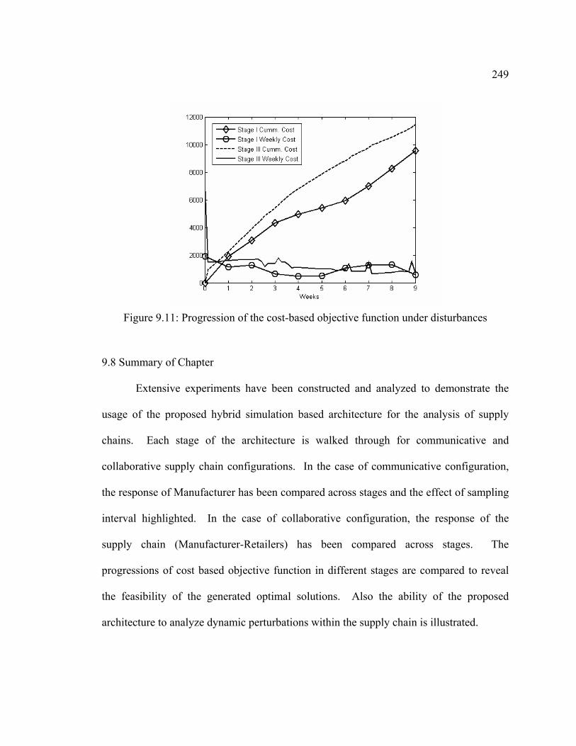
249

Figure 9.11: Progression of the cost-based objective function under disturbances

9.8 Summary of Chapter

Extensive experiments have been constructed and analyzed to demonstrate the

usage of the proposed hybrid simulation based architecture for the analysis of supply

chains. Each stage of the architecture is walked through for communicative and

collaborative supply chain configurations. In the case of communicative configuration,

the response of Manufacturer has been compared across stages and the effect of sampling

interval highlighted. In the case of collaborative configuration, the response of the

supply chain (Manufacturer-Retailers) has been compared across stages. The

progressions of cost based objective function in different stages are compared to reveal

the feasibility of the generated optimal solutions. Also the ability of the proposed

architecture to analyze dynamic perturbations within the supply chain is illustrated.

250

CHAPTER 10

CONCLUSIONS AND FUTURE RESEARCH

10.1 Summary of Research Work

The goal identified for this research is to analyze the interactions between the

planning decisions of different members of the supply chain, considering the operational

aspects at each member and the robustness of the plan. A three-echelon conjoined supply

chain consisting of a central Manufacturer, several Suppliers and Retailers, and a

transportation network is considered in this research. The generality of the proposed

architecture is discussed by considering two different configurations in the same supply

chain. Upstream to the Manufacturer, the supply chain structure is characterized as

communicative configuration. Downstream to the Manufacturer, the supply chain

structure is characterized as collaborative configuration of the type Vendor Managed

Inventory. Also, hierarchical production planning scheme is employed by the individual

members of the supply chain. An innovative approach of integrating and together

analyzing the distribution planning with the production planning decisions within a

supply chain environment is proposed.

The proposed architecture is divided into four stages: stability analysis (Stage I),

plan optimization (Stages II), schedule optimization (Stage III) and decision evaluation

(Stage IV). In Stage I the stability of the system is analyzed. If a supply chain is

unstable, it will experience large swings in demand, periods of shortage in materials and

products, periods of excess stock of materials, unpredictable lead times, all of which

251

affects the long term profits and success of the supply chain. Hence, the conditions for

the stability of the system response are established in relation to the various control

parameters of the model. The aggregated planning models, represented as a SD model,

capture the dynamic behavior and hence can be used to analyze the stability of the system.

In Stage II, the optimal set of control parameters for use in the decision policies of

the aggregate models are determined using non-linear optimization techniques. To make

the supply chain system operate in a stable regime the stability conditions, obtained

through stability analysis (Stage I), are employed as additional constraints within the

optimization model.

DES models capture the detailed operational activities at the Manufacturer,

Supplier, Retailer and Transporter. In Stage III, the optimal set of control parameters that

govern the flow of materials within the individual member units is determined using

meta-heuristic optimization techniques based on the production and distribution plan

obtained from Stage II.

In Stage IV, the optimality of the control parameters governing the aggregated

managerial policies (obtained from Stage II) and detailed operational policies (obtained

from Stage III) are concurrently evaluated using a hybrid system dynamic and discrete-

event modeling approach. In combined SD-DES model, the detailed operational

activities (materials flows) within the supply chain are captured using the DES models,

while the management decision policies based on the aggregated data (information flow)

are captured within the SD models. It is noted that the hybrid integrated models cannot

be directly used in stability analysis or optimization due to (1) the varied and often

252

conflicting objectives for the different members and the different levels (planning and

scheduling), (2) the complexity in building the models, especially the DES models that

contain the detailed operational activities of the members, and (3) time involved in

executing the entire distributed structure.

Extensive experiments had been constructed to demonstrate the usage of the

proposed hybrid simulation based architecture for the analysis of supply chains. Each

stage of the architecture had been walked through for the cases of communicative and

collaborative supply chain configurations. In the case of communicative configuration,

the response of Manufacturer had been compared across stages and the effect of sampling

interval highlighted. In the case of collaborative configuration, the response of the

supply chain (Manufacturer-Retailers) had been compared across stages. The

progressions of cost based objective function in different stages were compared to reveal

the feasibility of the generated optimal solutions. Also the ability of the proposed

architecture to analyze dynamic perturbations within the supply chain was illustrated.

In addition to the contribution of this research work on the development of an

architecture to enable distributed analysis of decision models spread across the supply

chain, this research work has made significant contributions in several topics including

(1) aggregate-level modeling, (2) stability analysis, (3) integrated analysis of performance

and stability, (4) interfacing scheme between SD and DES models, and (5)

implementation infrastructure enabling integration of distributed models. They are

summarized in the following sections.

253

10.1.1 Contributions in Aggregate-level Modeling

Generic aggregate-level system dynamic models that capture the mixing and

variability in the production process, capacitated resource allocation, and provides for

spatial and lateral dimension of the supply chain have been developed. The models

developed improve over the existing (prior research) models in the following aspects:

• Production process has been modeled as a higher order material delay, instead of a

fixed pipeline delay.

• Frequency of information update has been explicit modeled using sampling interval.

• Production capacity constraints were included.

• Order backlogs were maintained

• The products are composed of multiple components. Such lateral dimension creates a

consolidation of goods, which reflect the operations of typical supply chains.

• Retailer’s dispatching rule is based on a MIN-MAX inventory policy to mimic the

realistic operations at the retailer-level echelons of the supply chain.

• Spatial dimension of the supply chain has been created by modeling multiple

Suppliers (two) and multiple Retailers (three).

10.1.2 Contributions in Stability Analysis

The stability conditions for a general production ordering and inventory control

system was derived using z-transformation techniques. The system parameters included

fractional adjustment of WIP (α), fractional adjustment of inventory (β), exponential

254

smoothing constant for forecast (ρ), number of production stages (or order of production

delay) (Q), production lead time (L) and the sampling interval (δ). The stability

boundaries for system operating under inventory adequacy and inventory insufficiency

were established. The Jury’s Test has been employed to derive the stability conditions.

The effect of the frequency of information update on the stability of the

production-inventory system was analyzed. Results revealed that aggressive ordering

policies (higher values of the fractional adjustment rates for WIP and inventory) require a

more frequent information update, i.e. lower sampling interval.

Collaborative supply chain configuration employing vendor managed inventory

had been modeled and analyzed. The system parameters included adjustment rate for

goods-in-transit (ψ), adjustment rates for inventory levels at Retailers (φ), exponential

smoothing constant for forecasting demand (ρ), time to change the MIN and MAX levels

(τ), the product delivery lead time and the sampling intervals (δ and ∆).

The possible differences in the frequency of information update at the different

players and their effect on overall system stability was analyzed. For the case in which δ

= ∆, it was found that the smaller sampling interval settings of 1/7 (daily updates)

resulted in larger stability regions, thus allowing for a more aggressive ordering policy. It

was also found that frequent updates of information on the side of the Retailer (∆ < δ)

alone improves system wide performance (larger stability region). However, when the

Manufacturer makes updates more frequently than the Retailers (∆ > δ) no advantages are

gained. Hence it is desirable and could be cost effective for the Manufacturer to pace

255

their decisions equal or slower than the rate at which the Retailers can update the

information.

10.1.3 Contributions in Integrated Analysis of Performance and Stability

A novel method for the integration of the stability analysis with performance

analysis (optimization) has been presented by employing the stability conditions as

additional constraints within the optimization models. Designed experiments using

optimization was carried out to justify the use of stability constraints within the

optimization model.

10.1.4 Contributions in Interfacing SD and DES Models

In this research, a novel method of interfacing the models in different members of

the supply chain has been proposed, (1) without each member knowing the workings of

the entire supply chain, and (2) without revealing the members internal details to the rest

of the supply chain. This was achieved by ensuring that the member gives out and

receives data that mimics the activities in the real world. Also, a novel method of

interfacing SD and DES models for integrated analysis was presented. In the SD models,

the data for certain variables were obtained from the DES models at every sampling

interval. Thus the behavior of the entire supply chain is the result of complex inter-

relationships amongst the different models.

256

10.1.5 Contributions of Implementation Framework

A generic infrastructure using HLA/RTI has been developed to integrate and

together simulate the distributed simulation models. Reusable interface modules have

been implemented which can be used to quickly create distributed simulations with

multiple DES and/or multiple SD models. The developed interface modules are generic,

and hence can be used in any DES modeling package (Arena, ProModel, AutoMod) and

any SD modeling package (Vensim, Powersim, iThink). The only requirement for the

modeling package is that they must be able to communicate with external applications,

which is available in the most state-of-the-art software applications.

10.2 List of Firsts in the Research

• Created an environment for the distributed analysis of decision models spread across

the supply chain.

• Developed a comprehensive SD model for general production inventory system and

supply chain.

• Recognized the need to analyze the impact of the frequency of information updates

onto the stability of the supply chains.

• Created a method for combining stability with performance (optimization) analysis.

• Created a distributed simulation for supply chain analysis using commercial-off-the-

shelf simulation packages.

• Created hybrid distributed simulation for supply chain analysis, consisting of system

dynamic and discrete-event components.

257

10.3 Future Directions of Research

While this thesis has presented significant initial efforts towards the

understanding the effects of individual supply chain members on the entire supply chain,

there is still a great deal of work to be done. Extensions are possible in the

methodological aspects, technological aspects and the applications described in this

research.

The optimality of the various decision models are evaluated using distributed

simulation. How will we know that certain decisions are sub-optimal / infeasible? What

are the key indicators to be monitored? How will we know when to change the

decisions? These questions holds true during the planning / simulation stages in

analyzing supply chains, as well as during the execution stages of the supply chain.

The effect of information on the performance of the supply chain is to be

understood thoroughly. The role of information sharing is to be researched (Answers to

questions like: what information needs to be shared? How much information is to be

shared? How to use the information to optimize the goals of the supply chain? Is the

meaning of the information understood the same through out the supply chain?, etc need

to be sought after).

The effects of myopic and commonly-defined objectives of the supply chain

members were studied in this research. The consequence of possibly conflicting

objectives of different members of the supply chain on the overall system performance is

another area of interest.

258

From the perspective of technology, the distributed simulation based on HLA/RTI

requires a significant learning curve. Though attempts have been made to provide

simpler interfaces, it is still complex enough to prevent the wide-spread use of the

distributed simulation technology. Development of such simple interfaces is also of

potential interest. Investigation of the use of web services in this regard could be carried

out.

A generalized framework of simulation models could also be set-up, which can be

customized to any particular supply chain scenario and tested. The models could then be

verified with real data from real industries.

Varied applications for the proposed architecture are already underway. The

usage of the proposed framework for airport management system is being explored,

where the crew scheduling, flight scheduling, and maintenance scheduling are spread

across multiple airport and airlines. Also, the development of multi-level hierarchical

hybrid models to aid the understanding of biological behavior at the gene-level,

molecule-level, cell-level, organ-level and human level is of great interest and

opportunities.

259

APPENDIX A

Calculation of Processing Times for the Manufacturer’s Shop Floor

A reverse engineering approach has been employed to determine the processing

times and the shop floor specifications. It is decided that the Manufacturer must be

capable of producing at the rate of about 100 units/ week. Hence, a part must be

produced every 24*7/100 = 1.68 hours. Also, it was desired to have an average

production lead time of 3 weeks (21 days). Hence, according to Little’s law, the system

must carry an average WIP = 21*24/1.68 = 300 units. That is, 1 unit produced every 1.68

hours can be achieved by setting the production delay = 1.68 hours. For a production

lead time of 21 days, the parts need to be in the system for 21*24=504 hours. With 1.68

hours of processing times per machine, this would require 504/1.68 = 300 machines.

Now, the model is scaled by assuming a batch size of 10 and processing time = 16.8

hours per machine. This scales down the model to 504/16.8 = 30 machines.

The processing times (in hours) for all 30 machines are defined as Triangular

distribution (14 machines), Normal distribution (13 machines) or Uniform Distribution (3

machines). The means of the triangular and normal distributions have been generated

from UNIF[1.12, 1.76] using MinitabTM. Processing times 1.12 hours corresponds to a

production rate of 150 parts per week, and a time of 1.76 corresponds to production rate

of 90 parts week. The processing time distributions are presented in Table A.1.

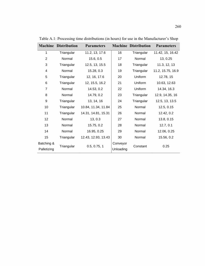
260

Table A.1: Processing time distributions (in hours) for use in the Manufacturer’s Shop

Machine Distribution Parameters Machine Distribution Parameters

1 Triangular 11.2, 13, 17.6 16 Triangular 11.42, 15, 16.42

2 Normal 15.6, 0.5 17 Normal 13, 0.25

3 Triangular 12.5, 13, 15.5 18 Triangular 11.3, 12, 13

4 Normal 15.28, 0.3 19 Triangular 11.2, 15.75, 16.9

5 Triangular 12, 16, 17.6 20 Uniform 12.78, 15

6 Triangular 12, 15.5, 16.2 21 Uniform 10.63, 12.63

7 Normal 14.53, 0.2 22 Uniform 14.34, 16.3

8 Normal 14.79, 0.2 23 Triangular 12.9, 14.35, 16

9 Triangular 13, 14, 16 24 Triangular 12.5, 13, 13.5

10 Triangular 10.84, 11.34, 11.84 25 Normal 12.5, 0.15


12 Normal 13, 0.3 27 Normal 13.8, 0.15

13 Normal 15.75, 0.2 28 Normal 12.7, 0.1

14 Normal 16.95, 0.25 29 Normal 12.06, 0.25


Batching &

Palletizing Triangular 0.5, 0.75, 1

Conveyor

UnloadingConstant 0.25

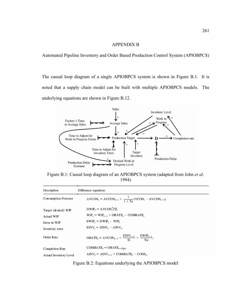
261

APPENDIX B

Automated Pipeline Inventory and Order Based Production Control System (APIOBPCS)

The causal loop diagram of a single APIOBPCS system is shown in Figure B.1. It is

noted that a supply chain model can be built with multiple APIOBPCS models. The

underlying equations are shown in Figure B.12.

Figure B.1: Causal loop diagram of an APIOBPCS system (adapted from John et al.

1994)

Figure B.2: Equations underlying the APIOBPCS model

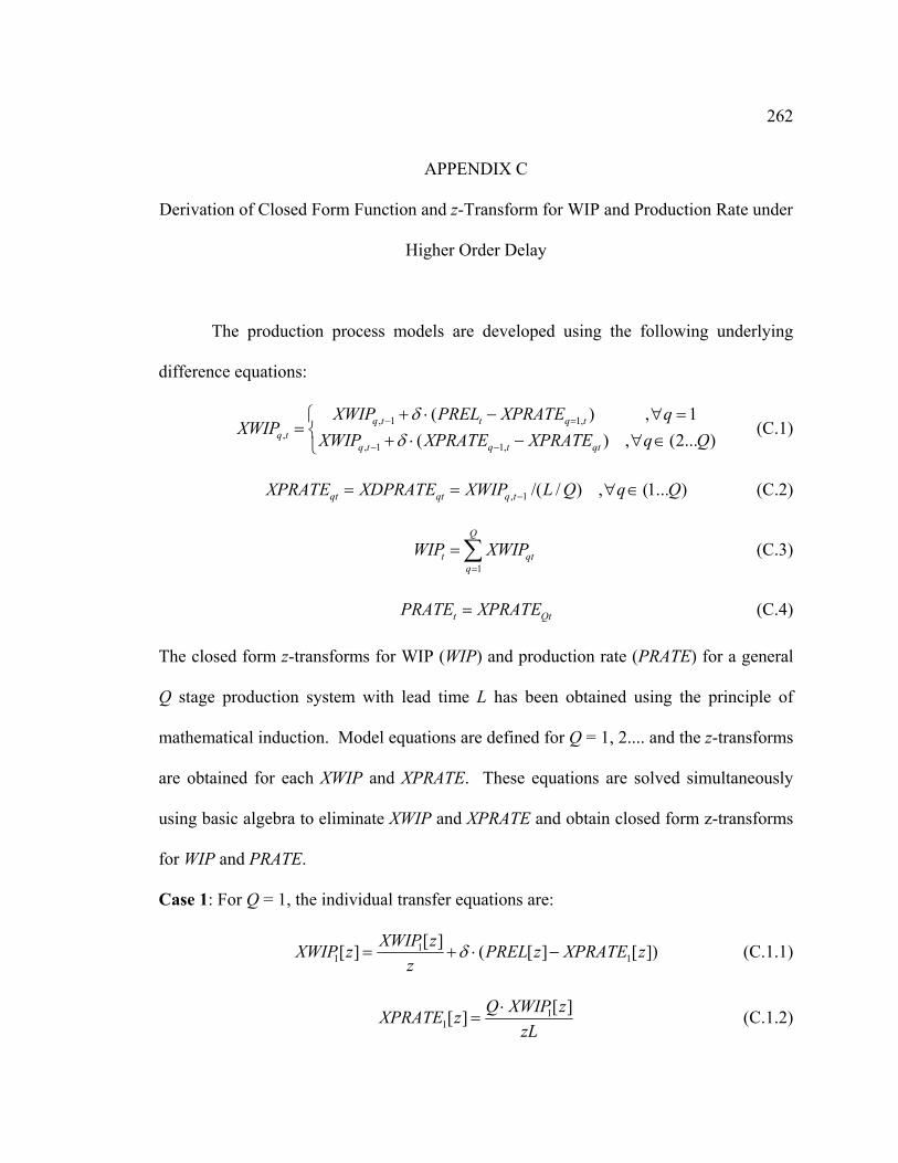
262

APPENDIX C

Derivation of Closed Form Function and z-Transform for WIP and Production Rate under

Higher Order Delay

The production process models are developed using the following underlying

difference equations:

, 1 1,,

, 1 1,

( )( ) , (2... )

q t t q tq t

q t q t qt

XWIP PREL XPRATE qXWIP

, 1XWIP XPRATE XPRATE q Q

δδ

− =

− −

+ ⋅ − ∀ =⎧= ⎨ + ⋅ − ∀ ∈⎩

(C.1)

, 1 /( / ) , (1... )qt qt q tXPRATE XDPRATE XWIP L Q q Q−= = ∀ ∈ (C.2)

(C.3) 1

Q

tq

WIP XWIP=

= ∑ qt

Qt tPRATE XPRATE= (C.4)

The closed form z-transforms for WIP (WIP) and production rate (PRATE) for a general

Q stage production system with lead time L has been obtained using the principle of

mathematical induction. Model equations are defined for Q = 1, 2.... and the z-transforms

are obtained for each XWIP and XPRATE. These equations are solved simultaneously

using basic algebra to eliminate XWIP and XPRATE and obtain closed form z-transforms

for WIP and PRATE.

Case 1: For Q = 1, the individual transfer equations are:

11 1

[ ][ ] ( [ ] [ ])XWIP zXWIP z PREL z XPRATE zz

δ= + ⋅ − (C.1.1)

11

[ ][ ] Q XWIP zXPRATE zzL

⋅= (C.1.2)

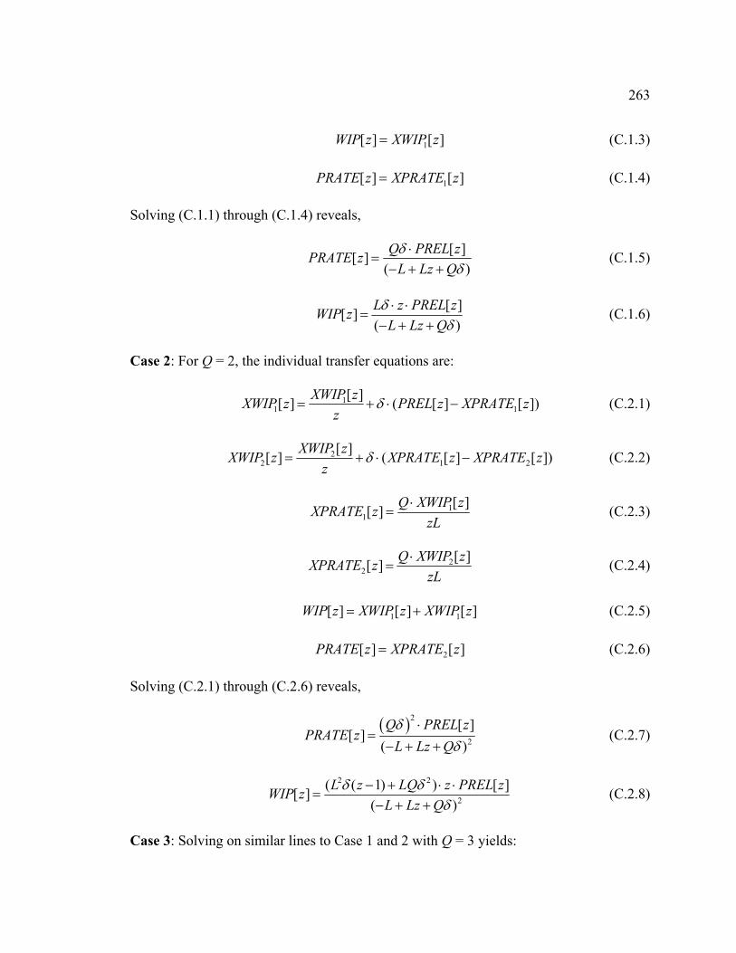
263

1[ ] [ ]WIP z XWIP z= (C.1.3)

1[ ] [ ]PRATE z XPRATE z= (C.1.4)

Solving (C.1.1) through (C.1.4) reveals,

[ ][ ]( )Q PREL zPRATE z

L Lz Qδ

δ⋅

=− + +

(C.1.5)

[ ][ ]( )L z PREL zWIP z

L Lz Qδ

δ⋅ ⋅

=− + +

(C.1.6)

Case 2: For Q = 2, the individual transfer equations are:

11 1

[ ][ ] ( [ ] [ ])XWIP zXWIP z PREL z XPRATE zz

δ= + ⋅ − (C.2.1)

22 1

[ ][ ] ( [ ] [ ])XWIP z2XWIP z XPRATE z XPRATE z

zδ= + ⋅ − (C.2.2)

11


⋅= (C.2.3)

22


⋅= (C.2.4)

1[ ] [ ] [ ]WIP z XWIP z XWIP z1= + (C.2.5)

2[ ] [ ]PRATE z XPRATE z= (C.2.6)

Solving (C.2.1) through (C.2.6) reveals,

( )2

2

[ ][ ]

( )Q PREL z

PRATE zL Lz Qδ

δ⋅

=− + +

(C.2.7)

2 2

2

( ( 1) ) [[ ]( )

L z LQ z PREL zWIP zL Lz Q

δ δδ

− + ⋅ ⋅=

− + +] (C.2.8)

Case 3: Solving on similar lines to Case 1 and 2 with Q = 3 yields:

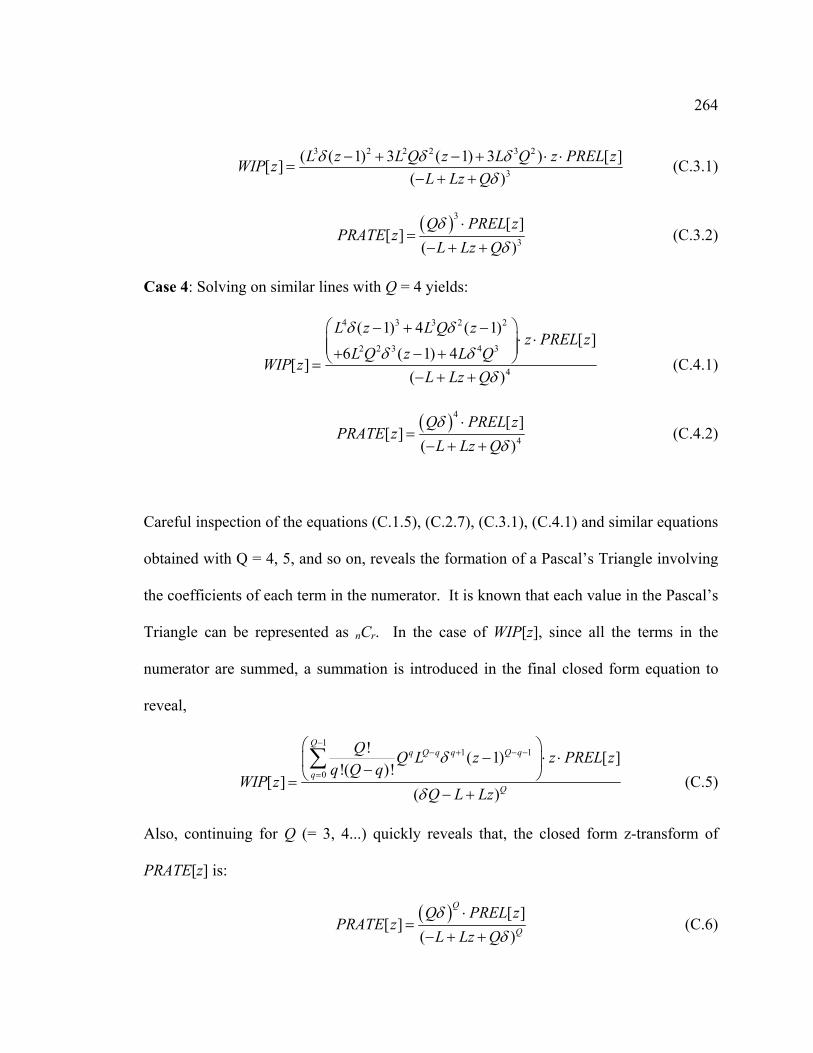
264

3 2 2 2 3 2

3

( ( 1) 3 ( 1) 3 ) [ ][ ]( )

L z L Q z L Q z PREL zWIP zL Lz Q

δ δ δδ

− + − + ⋅ ⋅=

− + + (C.3.1)

( )3

3

[ ][ ]

( )Q PREL z

PRATE zL Lz Qδ

δ⋅

=− + +

(C.3.2)

Case 4: Solving on similar lines with Q = 4 yields:

4 3 3 2 2

2 2 3 4 3

4

( 1) 4 ( 1)[ ]

6 ( 1) 4[ ]

( )

L z L Q zz PREL z

L Q z L QWIP z

L Lz Q

δ δ

δ δδ

⎛ ⎞− + −⋅ ⋅⎜ ⎟⎜ ⎟+ − +⎝ ⎠=

− + + (C.4.1)

( )4

4

[ ][ ]

( )Q PREL z

PRATE zL Lz Qδ

δ⋅

=− + +

(C.4.2)

Careful inspection of the equations (C.1.5), (C.2.7), (C.3.1), (C.4.1) and similar equations

obtained with Q = 4, 5, and so on, reveals the formation of a Pascal’s Triangle involving

the coefficients of each term in the numerator. It is known that each value in the Pascal’s

Triangle can be represented as nCr. In the case of WIP[z], since all the terms in the

numerator are summed, a summation is introduced in the final closed form equation to

reveal,

11 1

0

! ( 1) [ ]!( )!

[ ]( )

Qq Q q q Q q

qQ

Q Q L z z PREL zq Q q

WIP zQ L Lz

δ

δ

−− + − −

=

⎛ ⎞− ⋅ ⋅⎜ ⎟−⎝=

− +

∑⎠ (C.5)

Also, continuing for Q (= 3, 4...) quickly reveals that, the closed form z-transform of

PRATE[z] is:

( ) [ ][ ]

( )

Q

Q

Q PREL zPRATE z

L Lz Qδ

δ⋅

=− + +

(C.6)

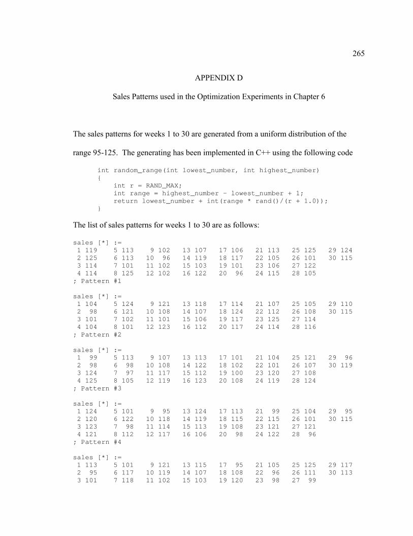
265

APPENDIX D

Sales Patterns used in the Optimization Experiments in Chapter 6

The sales patterns for weeks 1 to 30 are generated from a uniform distribution of the

range 95-125. The generating has been implemented in C++ using the following code

int random_range(int lowest_number, int highest_number) { int r = RAND_MAX; int range = highest_number - lowest_number + 1; return lowest_number + int(range * rand()/(r + 1.0)); }

The list of sales patterns for weeks 1 to 30 are as follows:

sales [*] := 1 119 5 113 9 102 13 107 17 106 21 113 25 125 29 124 2 125 6 113 10 96 14 119 18 117 22 105 26 101 30 115 3 114 7 101 11 102 15 103 19 101 23 106 27 122 4 114 8 125 12 102 16 122 20 96 24 115 28 105 ; Pattern #1 sales [*] := 1 104 5 124 9 121 13 118 17 114 21 107 25 105 29 110 2 98 6 121 10 108 14 107 18 124 22 112 26 108 30 115 3 101 7 102 11 101 15 106 19 117 23 125 27 114 4 104 8 101 12 123 16 112 20 117 24 114 28 116 ; Pattern #2 sales [*] := 1 99 5 113 9 107 13 113 17 101 21 104 25 121 29 96 2 98 6 98 10 108 14 122 18 102 22 101 26 107 30 119 3 124 7 97 11 117 15 112 19 100 23 120 27 108 4 125 8 105 12 119 16 123 20 108 24 119 28 124 ; Pattern #3 sales [*] := 1 124 5 101 9 95 13 124 17 113 21 99 25 104 29 95 2 120 6 122 10 118 14 119 18 115 22 115 26 101 30 115 3 123 7 98 11 114 15 113 19 108 23 121 27 121 4 121 8 112 12 117 16 106 20 98 24 122 28 96 ; Pattern #4 sales [*] := 1 113 5 101 9 121 13 115 17 95 21 105 25 125 29 117 2 95 6 117 10 119 14 107 18 108 22 96 26 111 30 113 3 101 7 118 11 102 15 103 19 120 23 98 27 99

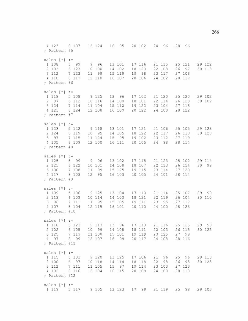
266

4 123 8 107 12 124 16 95 20 102 24 96 28 96 ; Pattern #5 sales [*] := 1 108 5 99 9 96 13 101 17 116 21 115 25 121 29 122 2 103 6 123 10 100 14 102 18 123 22 108 26 97 30 113 3 112 7 123 11 99 15 119 19 98 23 117 27 108 4 118 8 113 12 110 16 107 20 106 24 102 28 117 ; Pattern #6 sales [*] := 1 118 5 108 9 125 13 96 17 102 21 120 25 120 29 102 2 97 6 112 10 116 14 100 18 101 22 114 26 123 30 102 3 124 7 114 11 104 15 110 19 122 23 104 27 118 4 123 8 124 12 108 16 100 20 122 24 100 28 122 ; Pattern #7 sales [*] := 1 123 5 122 9 118 13 101 17 121 21 106 25 105 29 123 2 124 6 119 10 95 14 105 18 122 22 117 26 113 30 123 3 97 7 115 11 124 15 95 19 102 23 112 27 119 4 105 8 109 12 100 16 111 20 105 24 98 28 114 ; Pattern #8 sales [*] := 1 125 5 99 9 96 13 102 17 118 21 123 25 102 29 114 2 121 6 122 10 101 14 108 18 107 22 113 26 114 30 98 3 100 7 108 11 99 15 125 19 115 23 114 27 120 4 117 8 103 12 95 16 103 20 105 24 101 28 114 ; Pattern #9 sales [*] := 1 109 5 106 9 125 13 104 17 110 21 114 25 107 29 99 2 113 6 103 10 114 14 103 18 121 22 119 26 104 30 110 3 96 7 111 11 95 15 105 19 111 23 95 27 117 4 107 8 104 12 115 16 101 20 110 24 100 28 123 ; Pattern #10 sales [*] := 1 110 5 123 9 113 13 96 17 113 21 116 25 125 29 99 2 102 6 105 10 99 14 108 18 111 22 103 26 115 30 123 3 125 7 113 11 108 15 101 19 119 23 125 27 99 4 97 8 99 12 107 16 99 20 117 24 108 28 116 ; Pattern #11 sales [*] := 1 115 5 103 9 120 13 125 17 106 21 96 25 96 29 113 2 100 6 97 10 118 14 114 18 118 22 98 26 95 30 125 3 112 7 111 11 105 15 97 19 114 23 103 27 123 4 102 8 116 12 104 16 115 20 109 24 100 28 118 ; Pattern #12 sales [*] := 1 119 5 117 9 105 13 123 17 99 21 119 25 98 29 103

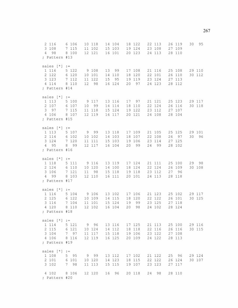
267

2 116 6 106 10 118 14 104 18 122 22 113 26 119 30 95 3 108 7 115 11 102 15 103 19 124 23 108 27 109 4 98 8 100 12 121 16 101 20 123 24 113 28 110 ; Pattern #13 sales [*] := 1 116 5 122 9 108 13 99 17 108 21 116 25 108 29 110 2 122 6 120 10 101 14 110 18 120 22 101 26 110 30 112 3 123 7 112 11 122 15 95 19 119 23 124 27 113 4 114 8 110 12 98 16 124 20 97 24 123 28 112 ; Pattern #14 sales [*] := 1 113 5 100 9 117 13 116 17 97 21 121 25 123 29 117 2 107 6 107 10 99 14 114 18 110 22 124 26 116 30 118 3 97 7 115 11 118 15 124 19 122 23 112 27 107 4 106 8 107 12 119 16 117 20 121 24 108 28 104 ; Pattern #15 sales [*] := 1 113 5 107 9 99 13 118 17 109 21 105 25 125 29 101 2 114 6 102 10 102 14 103 18 107 22 108 26 97 30 96 3 124 7 120 11 111 15 103 19 106 23 114 27 125 4 95 8 99 12 117 16 104 20 99 24 99 28 102 ; Pattern #16 sales [*] := 1 118 5 111 9 116 13 119 17 124 21 111 25 100 29 98 2 124 6 110 10 120 14 100 18 124 22 124 26 109 30 108 3 106 7 121 11 98 15 118 19 118 23 112 27 96 4 99 8 103 12 110 16 111 20 101 24 113 28 118 ; Pattern #17 sales [*] := 1 116 5 104 9 106 13 102 17 106 21 123 25 102 29 117 2 125 6 122 10 109 14 115 18 120 22 122 26 101 30 125 3 116 7 104 11 101 15 124 19 99 23 125 27 118 4 120 8 110 12 102 16 104 20 98 24 102 28 124 ; Pattern #18 sales [*] := 1 114 5 121 9 96 13 116 17 125 21 113 25 100 29 116 2 115 6 121 10 124 14 112 18 118 22 116 26 116 30 115 3 104 7 97 11 117 15 118 19 106 23 122 27 108 4 106 8 116 12 119 16 125 20 109 24 122 28 113 ; Pattern #19 sales [*] := 1 108 5 95 9 99 13 112 17 102 21 122 25 96 29 124 2 101 6 101 10 120 14 123 18 115 22 122 26 124 30 107 3 102 7 98 11 113 15 115 19 107 23 123 27 117 4 102 8 106 12 120 16 96 20 118 24 98 28 110 ; Pattern #20

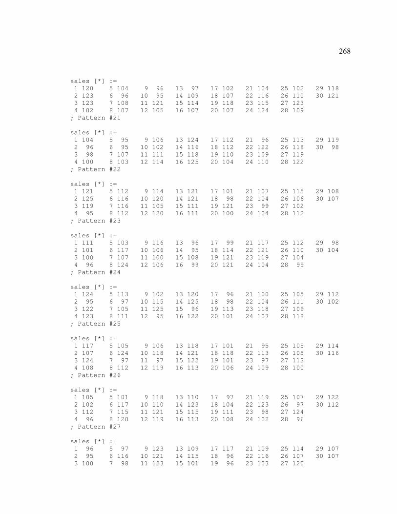
268

sales [*] := 1 120 5 104 9 96 13 97 17 102 21 104 25 102 29 118 2 123 6 96 10 95 14 109 18 107 22 116 26 110 30 121 3 123 7 108 11 121 15 114 19 118 23 115 27 123 4 102 8 107 12 105 16 107 20 107 24 124 28 109 ; Pattern #21 sales [*] := 1 104 5 95 9 106 13 124 17 112 21 96 25 113 29 119 2 96 6 95 10 102 14 116 18 112 22 122 26 118 30 98 3 98 7 107 11 111 15 118 19 110 23 109 27 119 4 100 8 103 12 114 16 125 20 104 24 110 28 122 ; Pattern #22 sales [*] := 1 121 5 112 9 114 13 121 17 101 21 107 25 115 29 108 2 125 6 116 10 120 14 121 18 98 22 104 26 106 30 107 3 119 7 116 11 105 15 111 19 121 23 99 27 102 4 95 8 112 12 120 16 111 20 100 24 104 28 112 ; Pattern #23 sales [*] := 1 111 5 103 9 116 13 96 17 99 21 117 25 112 29 98 2 101 6 117 10 106 14 95 18 114 22 121 26 110 30 104 3 100 7 107 11 100 15 108 19 121 23 119 27 104 4 96 8 124 12 106 16 99 20 121 24 104 28 99 ; Pattern #24 sales [*] := 1 124 5 113 9 102 13 120 17 96 21 100 25 105 29 112 2 95 6 97 10 115 14 125 18 98 22 104 26 111 30 102 3 122 7 105 11 125 15 96 19 113 23 118 27 109 4 123 8 111 12 95 16 122 20 101 24 107 28 118 ; Pattern #25 sales [*] := 1 117 5 105 9 106 13 118 17 101 21 95 25 105 29 114 2 107 6 124 10 118 14 121 18 118 22 113 26 105 30 116 3 124 7 97 11 97 15 122 19 101 23 97 27 113 4 108 8 112 12 119 16 113 20 106 24 109 28 100 ; Pattern #26 sales [*] := 1 105 5 101 9 118 13 110 17 97 21 119 25 107 29 122 2 102 6 117 10 110 14 123 18 104 22 123 26 97 30 112 3 112 7 115 11 121 15 115 19 111 23 98 27 124 4 96 8 120 12 119 16 113 20 108 24 102 28 96 ; Pattern #27 sales [*] := 1 96 5 97 9 123 13 109 17 117 21 109 25 114 29 107 2 95 6 116 10 121 14 115 18 96 22 116 26 107 30 107 3 100 7 98 11 123 15 101 19 96 23 103 27 120

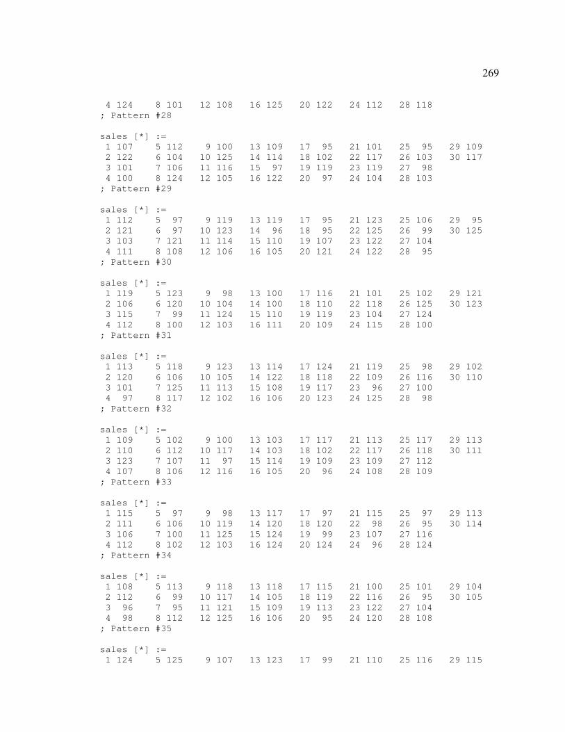
269

4 124 8 101 12 108 16 125 20 122 24 112 28 118 ; Pattern #28 sales [*] := 1 107 5 112 9 100 13 109 17 95 21 101 25 95 29 109 2 122 6 104 10 125 14 114 18 102 22 117 26 103 30 117 3 101 7 106 11 116 15 97 19 119 23 119 27 98 4 100 8 124 12 105 16 122 20 97 24 104 28 103 ; Pattern #29 sales [*] := 1 112 5 97 9 119 13 119 17 95 21 123 25 106 29 95 2 121 6 97 10 123 14 96 18 95 22 125 26 99 30 125 3 103 7 121 11 114 15 110 19 107 23 122 27 104 4 111 8 108 12 106 16 105 20 121 24 122 28 95 ; Pattern #30 sales [*] := 1 119 5 123 9 98 13 100 17 116 21 101 25 102 29 121 2 106 6 120 10 104 14 100 18 110 22 118 26 125 30 123 3 115 7 99 11 124 15 110 19 119 23 104 27 124 4 112 8 100 12 103 16 111 20 109 24 115 28 100 ; Pattern #31 sales [*] := 1 113 5 118 9 123 13 114 17 124 21 119 25 98 29 102 2 120 6 106 10 105 14 122 18 118 22 109 26 116 30 110 3 101 7 125 11 113 15 108 19 117 23 96 27 100 4 97 8 117 12 102 16 106 20 123 24 125 28 98 ; Pattern #32 sales [*] := 1 109 5 102 9 100 13 103 17 117 21 113 25 117 29 113 2 110 6 112 10 117 14 103 18 102 22 117 26 118 30 111 3 123 7 107 11 97 15 114 19 109 23 109 27 112 4 107 8 106 12 116 16 105 20 96 24 108 28 109 ; Pattern #33 sales [*] := 1 115 5 97 9 98 13 117 17 97 21 115 25 97 29 113 2 111 6 106 10 119 14 120 18 120 22 98 26 95 30 114 3 106 7 100 11 125 15 124 19 99 23 107 27 116 4 112 8 102 12 103 16 124 20 124 24 96 28 124 ; Pattern #34 sales [*] := 1 108 5 113 9 118 13 118 17 115 21 100 25 101 29 104 2 112 6 99 10 117 14 105 18 119 22 116 26 95 30 105 3 96 7 95 11 121 15 109 19 113 23 122 27 104 4 98 8 112 12 125 16 106 20 95 24 120 28 108 ; Pattern #35 sales [*] := 1 124 5 125 9 107 13 123 17 99 21 110 25 116 29 115

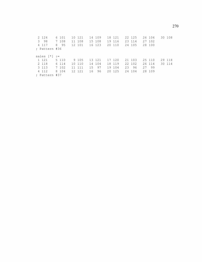
270

2 124 6 101 10 121 14 109 18 121 22 125 26 104 30 108 3 98 7 108 11 108 15 108 19 116 23 114 27 102 4 117 8 95 12 101 16 123 20 110 24 105 28 100 ; Pattern #36 sales [*] := 1 121 5 110 9 105 13 121 17 120 21 103 25 110 29 118 2 118 6 114 10 110 14 104 18 119 22 102 26 114 30 114 3 113 7 102 11 111 15 97 19 104 23 96 27 99 4 112 8 104 12 121 16 96 20 125 24 104 28 109 ; Pattern #37

271

APPENDIX E

Installing and Executing the RTI and DMS Adapter

E.1 Installations required

DMS Adapter is used as an interface between the simulation models and the HLA

RTI. The ‘DMSAdapter.dll’, ‘DMSAdapter.fed’, ‘RTI.rid’ and ‘DMSDebugLog.exe’ are

the essential files of the adapter. The ‘DMSAdapter.dll’ is a dynamic link library. It

implements all the functions required of the adapter2. It needs to be called on as a

reference object of Visual Basic editor to make use of the functions. ‘DMSAdapter.fed’

is the federation file that needs to be used with the adapter. The ‘RTI.rid’ file contains

the parameters for setting connection between adapter and the RTI. The

‘DMSDebugLog.exe’ shows the status of the interaction between the adapter and the RTI.

To install, unzip the file ‘Distribution.zip’. Go to the bin sub-folder in the

installed directory. Use ‘RegisterAdapter.bat’ to register the ‘DMSAdapter.dll’. The dll

must be registered. If a “Load Library Failure” error occurs, try to unzip the dll’s from

‘MSNT4dll’s.zip’ into the bin directory. A problem would still be encountered if the

HLA-RTI is not installed in that computer. To over come that, copy the dll’s ‘aced.dll’,

‘libFedTimed.dll’, ‘libRTI-NGd.dll’, ‘orbsvcsd.dll’, and ‘TAOd.dll’ into the bin directory.

These dll’s can be found in the bin sub-directory of the RTI installed directory. The use

of these dll’s helps to install and run the adapter without installing the HLA RTI in that

computer. After successful registration of the ‘DMSAdapter.dll’ run ‘RegDebugLog.bat’,

2 Refer the Distributed Manufacturing Simulation Reference Guide.

272

located in the DebugLog sub-directory, to register the DMSDebugLog. Then create and

set the environment variable RTI_RID_FILE to the ‘RTI.rid’ file located in the bin

directory. For example, the following might be the path for the rid file:

"c:\distribution\bin\RTI.rid". Now the adapter is ready to be used in conjunction with the

simulation models.3

The HLA RTI software can be downloaded and installed from the site

"http://sdc.dmso.mil/". For installation instructions refer to the installation guide provide

during download.

E.2 Executing the RTI

If all federates are running in the same LAN, then the RTI must be started as:

command prompt> rtiexec.exe -multicastDiscoveryEndpoint 224.1.2.3:12345

The ‘rtiexec.exe’ is the RTI. The numbers 224.1.2.3:12345 refer to the IP-address and

port of that RTI. It need not be the actual IP address of the computer on which the RTI is

running. Using different IP-address: port configurations, more than one RTI can be run

on the same LAN. Also in the ‘RTI.rid’ file the following line must be added:

(RtiExecutiveMulticastDiscoveryEndpoint 224.1.2.3:12345)

The IP-address: port specified in this file must be the same as the one used to start the

RTI.

If the federates are running over a WAN or the Intranet, then the RTI must be

started as:

3 More instructions on installing are found in the documentation sub-folder.

273

command prompt>rtiexec -endpoint juno.sie.arizona.edu:12345

juno.sie.arionz.edu:12345 refers to the actual IP address of the computer on which the

RTI is running. Then, in the ‘RTI.rid’ file, the line:

(RtiExecutiveEndpoint 128.196.219.197:12345)

must be added. This line must be commented out or removed when the RTI is running

within the LAN.

When the simulation starts, it checks the ‘RTI.rid’ file. If it finds the

‘RtiExecutiveEndpoint’, then it tries to connect to the RTI running on the computer with

the IP-address specified. If the ‘RtiExecutiveEndpoint’ is not specified, the simulation

searches the entire LAN and tries to connect with the RTI whose IP-address:port is

specified in the ‘RTI.rid’ file’s ‘RtiExecutiveMulticastDiscoveryEndpoint’.

274

REFERENCES

ADELSON, R. M., 1966, The dynamic behaviour of linear forecasting and scheduling rules. Operational Research Quarterly, 17(4), 447-462.

ARI, E. A. and AXSÄTER, S., 1988, Disaggregation under uncertainty in hierarchical production planning. European Journal of Operations Research, 35, 182-186.

AXSÄTER, S., 1985, Control theory concepts in production and inventory control. International Journal of Systems Science, 16, 161–169.

BEAMON, B. M. and CHEN, V. C. P., 2001, Performance analysis of conjoined supply chains. International Journal of Production Research, 39(14), 3195-3218.

BINDER, T., VOX, A., BELYAZID, S., HARALDSSON, H., and SVENSSON, M., 2004, Developing System Dynamics Models from Causal Loop Diagrams. Proceedings of the 22nd International Conference of the System Dynamics Society, Oxford.

BISSELL, C. C., 1996, Control Engineering (London: Chapman & Hall).

BONEY, M. C., POPPLEWELL, K. and MATOUG, M., 1994, Effect of errors and delays in inventory reporting on production system performance. International Journal of Production Research, 35, 93-105.

BURNS, J. R., 2001, Simplified translation of CLDs into SFDs. Proceedings of the 19th International Conference of the System Dynamics Society, Atlanta, GA.

BYRNE, M. D. and BAKIR, M. A., 1999, Production planning using a hybrid simulation – analytical approach. International Journal of Production Economics, 59, 305-311.

CACHON, G. and FISHER, M., 1997, Campbell soup’s continuous replenishment program: evaluation and enhanced inventory decision rules. Production and Operations Management, 6(3), 266-276.

COYLE, R. G., 1977, Management System Dynamics (New York: John Wiley & Sons).

DANGERFIELD, B. and ROBERTS, C., 1996, An Overview of Strategy and Tactics in System Dynamic Optimization. The Journal of Operational Research Society, 47(3), 405-423.

DAS, B. P., RICKARD, J. G., SHAH, N. and MACCHIETTO, S., 2000, An investigation on integration of aggregate production planning, master production scheduling and short-term production scheduling of batch process operations through a common data model. Computers and Chemical Engineering, 44, 63-72.

275

DEJONCKHEERE, J., DISNEY, S. M., LAMBRECHT, M. and TOWILL, D. R., 2003, The dynamics of aggregate planning. Production Planning & Control, 14(6), 497-516.

DEZIEL, D. P. and EILON, S., 1967, A linear production-inventory control rule. The Production Engineer, 43, 93-104.

DISNEY, S. M., 2001. The production and inventory control problem in vendor managed inventory supply chains. Ph.D. Thesis, Cardiff Business School, Cardiff University.

DISNEY, S. M., HOLMSTRÖM, J., KAIPIA, R. and TOWILL, D.R., 2001, Implementation of a VMI production and distribution control system. International Symposium of Logistics.

DISNEY, S. M., NAIM, M. M. and TOWILL, D. R., 2000, Genetic algorithm optimization of a class of inventory control systems. International Journal of Production Economics, 68, 259–278.

DISNEY, S. M., POTTER, A. T. and GARDNER, B. M., 2003, The Impact of Vendor Managed Inventory on Transport Operations. Transport Research Part E, 39, 363-380.

DISNEY, S. M. and TOWILL, D. R., 2002, A Discrete Transfer Function Model to Determine the Dynamic Stability of a Vendor Managed Inventory Supply Chain. International Journal of Production Research, 40(1), 179-204.

DISNEY, S. M. and TOWILL, D. R., 2005, Eliminating drift in inventory and order based production control systems. International Journal of Production Economics, 93-94, 331-344.

DISNEY, S. M., TOWILL, D. R. and VAN DE VELDE, W., 2004, Variance amplification and the golden ratio in production and inventory control. International Journal of Production Economics, 90(3), 295-309.

DMS Adapter Reference Guide, 2001, National Institute of Technology and Science.

DONG, Y. and XU, K., 2002, A supply chain model of vendor managed inventory. Transportation Research Part E: Logistics and Transportation Review, 38(2), 75-95.

EDGHILL, J. and TOWILL, D. R., 1990, Assessing manufacturing system performance: frequency response revisited. Engineering Costs and Production Economics, 19, 319–326.

FORRESTER, J. W., 1961, Industrial Dynamics (Cambridge: MIT Press).

FU, M. C., 2002, Optimization for simulation: theory vs. practice. Informs Journal on Computing, 14(3), 192–215.

FUJIMOTO, R. M., 2000, Parallel and Distributed Simulation Systems (Wiley InterScience).

276

GANESHAN, R. and HARRISON, T. P., 1993, An introduction to supply chain management. Available online via <http://silmaril.smeal.psu.edu/misc/ supply_chain_intro.html> [accessed November 1, 2001].

GLOVER, F., KELLY, J. P. and LAGUNA, M., 1999, The OptQuest Callable Library User’s Documentation, Optimization Technologies Inc., Boulder, CO.

GRUBBSTRÖM, R. W., 1998, A net present value approach to safety stocks in planned production, International Journal of Production Economics, 56(7), 213–229.

GRUBBSTRÖM, R. W. and WIKNER, J., 1996, Inventory trigger control policies developed in terms of control theory. International Journal of Production Economics, 45, 397–406

HAX, A. C. and MEAL, H. C., 1975, Hierarchical integration of production planning and scheduling. In M. A. Geisler (ed), Studies in the Management Sciences, Vol. 1, Logistics, (New York: North-Holland American Elsevier), 53-69

HOLMSTRÖM, J., FRÄMLING, K., KAIPIA, R. and SARANEN, J., 2002, Collaborative Planning, Forecasting and Replenishment: New solutions needed for mass collaboration. Supply Chain Management: An International Journal, 7(3), 136-145.

JAFFERALI, M., VENKATESWARAN, J. and SON, Y., 2005, Performance Comparison of Search-based Simulation Optimization Algorithms for Operations Scheduling, International Journal of Simulation and Process Modeling, 1(1~2), 58-71.

JOHN, S., NAIM, M. M. and TOWILL, D. R., 1994, Dynamic analysis of a WIP compensated decision support system. International Journal of Manufacturing System Design, 1(4), 283-297.

JURY, E. I., 1964, Theory and Application of the z-Transform Method (New York: Robert E. Krieger).

KAACUTEDAACUTER, B., MONOSTORI, L. and SZELKE, E., 1998, An object-oriented framework for developing distributed manufacturing architectures. Journal of Intelligent Manufacturing, 9(2), 173-179.

KATAYAMA, H., 1996, On a two-stage hierarchical production planning system for process industries. International Journal of Production Economics, 59, 305-311.

KELTON, W. D., SADOWSKI, R. P. and SADOWSKI, D. A., 1997, Simulation with Arena. 1st Ed (New York: McGraw-Hill).

KELTON, W. D., SADOWSKI, R. P. and SADOWSKI, D. A., 2001, Simulation with Arena. 2nd Ed (New York: McGraw-Hill).

277

KUHL, F., WEATHERLY, R. and DAHMANN, J., 1999, Creating Computer Simulations: An Introduction to the High Level Architecture (Upper Saddle River, NJ: Prentice-Hall).

LAMBERT, D. M., COOPER, M. C. and PUGH, J .D., 1998, Supply chain management: implementation issues and research opportunities. International Journal of Logistics Management, 9(2), 1-19.

LEE H. L. and BILLINGTON, C., 1993, Materials management in decentralized supply chain. Operations Research, 41(5), 835-847.

LEE, H. L., PADMANABHAN, V. and WHANG, S., 1997, Information distortion in a supply chain: the bullwhip effect. Management Science, 43(4), 546-558.

LEE, Y. H., CHO, M. K. and KIM, Y. B., 2002, A Discrete-Continuous Combined Modeling Approach for Supply Chain Simulation. Simulation, 78(5), 321-329.

LEE, Y. H. and KIM S. H., 2002, Production–distribution planning in supply chain considering capacity constraints. Computers & Industrial Engineering, 43(1), 169-190.

LEONG, G. K., OLIFF, M. D. and MARKLAND, R. E., 1989, Improved hierarchical production planning, Journal of Operations Management, 8(2), 90-114.

MABERT, V. A. and VENKATARAMANAN, M. A., 1998, Special research focus on supply chain linkage: challenges for design and management in the 21st century. Decision Sciences, 29(3), 537-552.

MAIONE, B. and NASO, D., 2001, Evolutionary adaptation of dispatching agents in heterarchical manufacturing systems. International Journal of Production Research, 39(7), 1481-1503.

MCKAY, K. N. and WIERS, V. C. S., 2003, Integrated decision support for planning, scheduling and dispatching tasks in a focused factory. Computers in Industry, 50, 5-14.

MCLEAN, C. and RIDDICK, F., 2000, The IMS Mission architecture for distributed manufacturing simulation. Proceedings of the Winter Simulation Conference (Orlando, FL), 1540-1548.

MEHRA, A., MINIS, I. and PROTH, J. M., 1996, Hierarchical production planning for complex manufacturing systems. Advances in Engineering Software, 26, 209-218.

MOHANTY, R. P. and KULKARNI, R. V., 1987, Hierarchical production planning: comparison of some heuristics, Engineering Costs and Production Economics, 11, 203-214.

NORAN, O. S., 2004, Business Modeling: UML vs IDEF, School of Computing and Information Technology, Griffith University, Australia. Available online at

278

<http://www.cit.gu.edu.au/~noran/Docs/UMLvsIDEF.pdf> [accessed August 3, 2003]

ORTEGA, M. and LIN, L., 2004, Control Theory Applications to the Production-Inventory Problem: A Review. International Journal of Production Research, 42(11), 2303-2322.

PANWALKER, S. S. and ISKANDER, W., 1977, A survey of scheduling rules. Operations Research, 25(1), 45–61.

PETROPOULAKIS, L. and GIACOMINI, L., 1998, Development of Hybrid Simulator for Manufacturing Process. Computers in Industry, 36, 117-124.

QUI, M. M. and BURCH, E. E., 1997, Hierarchical production planning and scheduling in a multi-product, multi-machine environment. International Journal of Production Research, 35(11), 3023-3042.

RABELO, L., HELAL, M., JONES, A., MIN, J., SON, Y. J. and DESHMUKH, A., 2003, A hybrid approach to manufacturing enterprise simulation. Proceedings of the Winter Simulation Conference (New Orleans, LA), 1125-1133.

REID, R. A. and KOLJONEN, E. L., 1999, Validating a manufacturing paradigm: a system dynamics modeling approach. Proceedings of the 1999 Winter Simulation Conference (Phoenix, AZ), 759–765.

RICHARDSON, G. P. 1986. Problems with Causal Loop Diagrams. System Dynamics Review, 2(2) (Summer): 158-170.

RICHARDSON, G. P. 1997. Problems in Causal Loop Diagrams Revisited. System Dynamics Review, 13(3) (Summer): 247-252.

SCHNEEWEISS, C., 2003, Hierarchies in Distributed Decision Making, 2nd edn (Berlin: Springer).

SETHI, S. P., TAKSAR, M. and ZHANG, Q., 1995, Hierarchical capacity expansion and production planning decisions in stochastic manufacturing systems. Journal of Operations Management, 12, 331-352.

SETHI, S. P., ZHANG, H. and ZHANG, Q., 2000, Hierarchical production control in a stochastic N-machine flowshop with limited buffers. Journal of Mathematical Analysis and Applications, 246, 28-57.

SIMATUPANG, T.M. and SRIDHARAN, R., 2002, The collaborative supply chain. International Journal of Logistics Management, 13(1), 15-30.

279

SON, Y., JOSHI, S. B., WYSK, R. A. and SMITH, J. S., 2002, Simulation Based Shop Floor Control. Journal of Manufacturing Systems, 21(5), 380 - 394.

SRINIVASA RAGAVAN, N. R. and VISWANATHAN, N., 2001, Generalized queuing network analysis of integrated supply chains. International Journal of Production Research, 39(2), 205-224.

STERMAN, J. D. 2000. Business Dynamics (Boston: MA: Mc-Graw Hill).

SWAMINATHAN, J. M., SMITH, S. F. and SADEH, N. M., 1995, Modeling the dynamics of supply chains. The Robotics Institute, Carnegie Mellon University, Pittsburg, Pennsylvania.

TANG, O. and NAIM, M. M., 2004, The Impact of Information Transparency on the Dynamic Behaviour of a Hybrid Manufacturing/Remanufacturing System. International Journal of Production Research, 42(19), 4135–4152.

TAYLOR, S. J. E., SUDRA, R., JANAHAN, T., TAN, G. and JOHN, L., 2002, An infrastructure for distributed supply chain simulation. Simulation, 78(5), 312-320.

TOWILL, D. R., 1982, Dynamic analysis of an inventory and order based production control system. International Journal of Production Research, 20, 671–687.

TOWILL, D. R., 1991, Supply chain dynamics. International Journal of Computer Integrated Manufacturing, 4(4), 197-208.

TOWILL, D. R., EVANS, G. N. and CHEEMA, P., 1997, Analysis and design of an adaptive minimum reasonable inventory control system. Production Planning and Control, 8, 545–557.

TSUBONE, H. and FURUTA, H., 1996, Replanning timing in hierarchical production planning. International Journal of Production Economics, 44, 53-61.

VENKATESWARAN, J. and SON, Y., 2004a, Impact of modelling approximations in supply chain analysis – an experimental study, International Journal of Production Research, 42(15), 2971-2992.

VENKATESWARAN, J. and SON, Y., 2004b, Design and Development of a Prototype Distributed Simulation for Evaluation of Supply Chains. International Journal of Industrial Engineering, 11(2), 151 – 160.

VENKATESWARAN, J. and SON, Y., 2004c, Distributed and hybrid simulations for manufacturing systems and integrated enterprise. Proceedings of the 2004 Industrial Engineering Research Conference (Houston, TX).

280

VENKATESWARAN, J. and SON, Y., 2004d, Hybrid System Dynamic – Discrete Event Simulation based Architecture for Hierarchical Production Planning. International Journal of Production Research, (submitted)

VENKATESWARAN, J., SON, Y. and JONES, A., 2004, Hierarchical production planning using a hybrid system dynamic-discrete event simulation architecture. Proceedings of the Winter Simulation Conference (Washington, D.C.).

VASSIAN, H. J., 1954, Application of discrete variable servo theory to inventory control. Journal of the Operations Research Society of America, 3(3), 272-282.

VICENS, E., ALEMANY, A. E., ANDRÉS, C. and GUARCH, J. J., 2001, A design and application methodology for hierarchical production planning decision support systems in an enterprise integration context. International Journal of Production Economics, 74, 5-20.

WHITE, A. S., 1999, Management of inventory using control theory. International Journal of Technology Management, 17, 847–860.

WIKNER, J., NAIM, M. M. and TOWILL, D. R., 1992, The system simplification approach in understanding the dynamic behaviour of a manufacturing supply chain. Journal of Systems Engineering, 2, 164–178.

YAN, H. S., 1997, An interaction/prediction approach to hierarchical production planning and control with delay interaction equations. Computer Integrated Manufacturing Systems, 10(4), 309-320.

ZEIGLER, B. P. and SARJOUGHIAN, H. S., 2000, Creating distributed simulation using DEVS M&S environments. Proceedings of the Winter Simulation Conference (Orlando, FL), 158-160.

PRODUCTION AND DISTRIBUTION PLANNING FOR...

Documents

Transcript of PRODUCTION AND DISTRIBUTION PLANNING FOR...