Mathematical Programming manuscript No.(will be inserted by the editor)

Roman A. Polyak

Primal-Dual Lagrangian Transformation method for Convex

Optimization

Received: date / Revised version: date

Abstract. A class Ψ of strongly concave and smooth functions ψ : R → R with specific properties is used to transform

the terms of the classical Lagrangian associated with the constraints. The transformation is scaled by a positive vector of

scaling parameters, one for each constraint.

Each step of the Lagrangian Transformation (LT) method alternates unconstrained minimization of LT in primal space

with both Lagrange multipliers and scaling parameters update.

Our main focus is on the primal-dual LT method. We introduce the primal-dual LT method and show that under the

standard second order optimality condition the method generates a primal-dual sequence that globally converges to the

primal-dual solution with asymptotic quadratic rate.

Key words. Lagrangian transformation – duality – interior quadratic prox – primal-dual LT method

1. Introduction

We replace the unconstrained minimization of the LT in the primal space and the Lagrange multipliers

update by solving the primal-dual (PD) system of equations. The application of Newton method to the

PD system leads to the primal-dual LT (PDLT) method, which is our main focus.

By solving the PD system a given vector of Lagrange multipliers is mapped into a new primal-dual

pair, while the scaling parameters vector remains fixed. The contractibility properties of the corresponding

map are critical for both the convergence and the rate of convergence. To understand the conditions under

which the corresponding map is contractive and to find the contractibility bounds one has to analyze the

primal-dual maps (see [18]–[20]). It should be emphasized that neither the primal LT sequence nor the

dual sequence generated by the Interior Quadratic Prox method provides sufficient information for this

Roman A. Polyak: Department of SEOR and Mathematical Sciences Department, George Mason University, 4400 University

Dr, Fairfax VA 22030, rpolyak@gmu.edu

Mathematics Subject Classification (1991): 20E28, 20G40, 20C20

2 Roman A. Polyak

analysis. Only the PD system, solving which is equivalent to one LT step, has all necessary components for

such analysis. This reflects the important observation that for any multipliers method neither the primal

nor the dual sequences control the computational process. The numerical process is governed rather by

the PD system. The importance of the PD system associated with nonlinear rescaling methods has been

recognized for quite some time (see [18],[19]).

Recently, the corresponding PD systems were used to develop globally convergent primal-dual non-

linear rescaling methods with an up to 1.5-Q superlinear rate (see [23], [24] and references therein).

In this paper we introduce a general primal-dual LT method. The method generates a globally con-

vergent primal-dual sequence, which, under the standard second order optimality condition converges to

the primal-dual solution with asymptotic quadratic rate. This is our main contribution.

In the initial phase, the PDLT works as the Newton LT method, i.e. Newton method for LT min-

imization followed by the Lagrange multipliers and the scaling parameters update. At some point, the

Newton LT method automatically turns into the Newton method for the Lagrange system of equations

corresponding to the active constraints. We would like to emphasize that the PDLT is not a mechanical

combination of two different methods. It is rather a universal procedure, which computes at each step

a primal-dual direction. Then, dependent on the reduction rate of the merit function, it uses either the

primal direction to minimize the LT in primal space or the primal-dual direction to reduce the merit

function value. In many aspects it is reminiscent of the Newton method with step-length for smooth

unconstrained optimization.

This similarity is due to:

1) the special properties of ψ∈Ψ ;

2) the structure of the LT method, in particular, the way in which the Lagrange multipliers and

scaling parameters are updated at each step;

3) the fact that the Lagrange multipliers corresponding to the passive constraints converge to zero

with at least quadratic rate;

4) the way in which we use the merit functions for updating the penalty parameter;

5) the way in which we employ the merit function for the Lagrangian regularization.

Primal-Dual Lagrangian Transformation method for Convex Optimization 3

It should be emphasized that the PDLT is free from any stringent conditions on accepting the Newton

step, which are typical for constrained optimization problems.

There are three important features that make Newton method for the primal-dual LT system free

from such restrictions.

First, the LT is defined on the entire primal space.

Second, after a few Lagrange multipliers updates the terms of the LT corresponding to the passive

constraints become negligibly small due to the at least quadratic convergence to zero of the Lagrange

multipliers corresponding to the passive constraints. Therefore, on the one hand, these terms became

irrelevant for finding the Newton direction. On the other hand, there is no need to enforce their nonneg-

ativity.

Third, the LT multipliers method is, generally speaking, an exterior point method in the primal space.

Therefore there is no need to enforce the nonnegativity of the the slack variables for the active constraints

as takes place in the Interior Point Methods (see [28]).

After a few Lagrange multipliers updates, the primal-dual LT direction becomes practically identical

to the Newton direction for the Lagrange system of equations corresponding to the active constraints.

This makes it possible to prove the asymptotic quadratic convergence of the primal-dual sequence.

The paper is organized as follows. In the next section we state the problem and introduce the basic

assumptions on the input data. In section 3 we formulate the general LT method and describe some

convergence results, which will be used later. In section 4 we introduce the Primal-Dual LT method and

prove its local quadratic convergence under the standard second order optimality conditions. In section

5 we consider the globally convergent primal-dual LT method and show that the primal-dual sequence

converges with an asymptotic quadratic rate. We conclude the paper with some remarks concerning future

research.

4 Roman A. Polyak

2. Statement of the problem and basic assumptions

Let f : Rn → R1 be convex and all ci : Rn → R1, i = 1, . . . , q, be concave and smooth functions. We

consider the following convex optimization problem:

x∗ ∈ X∗ = Argminf(x) | x ∈ Ω, (P )

where Ω = x : ci(x) ≥ 0, i = 1, . . . , q. We assume that:

A: The optimal set X∗ is nonempty and bounded.

B: Slater’s condition holds , i.e. there exists

x : ci(x) > 0, i = 1, . . . , q.

Let us consider the Lagrangian L(x, λ) = f(x)−∑q

i=1 λici(x), the dual function

d(λ) = infx∈Rn

L(x, λ)

and the dual problem

λ ∈ L∗ = Argmaxd(λ) | λ∈Rq+. (D)

Due to assumption B, the Karush-Kuhn-Tucker (KKT) conditions hold true, i. e. there exists a vector

λ∗ = (λ∗1, . . . , λ∗q) ∈ Rq

+ such that

∇xL(x∗, λ∗) = ∇f(x∗)−q∑

i=1

λ∗i∇ci(x∗) = 0 (1)

and the complementary slackness conditions

λ∗i ci(x∗) = 0, i = 1, . . . , q (2)

are satisfied.

We assume that the active constraint set at x∗ is I∗ = i : ci(x∗) = 0 = 1, . . . , r, r < n. Let us

consider the vector-functions cT (x) = (c1(x), . . . , cq(x)), cT(r)(x) = (c1(x), . . . , cr(x)) and their Jacobians

∇c(x) = J(c(x)) and ∇c(r)(x) = J(c(r)(x)).

The sufficient regularity condition

rank∇c(r)(x∗) = r, λ∗i > 0, i ∈ I∗ (3)

Primal-Dual Lagrangian Transformation method for Convex Optimization 5

together with the sufficient condition for the minimum x∗ to be isolated

(∇2xxL(x∗, λ∗)y, y) ≥ µ(y, y), µ > 0 ∀y 6= 0 : ∇c(r)(x∗)y = 0 (4)

comprise the standard second order optimality condition.

3. Lagrangian transformation method.

We consider a class Ψ of twice continuous differentiable functions ψ : (−∞,∞) → R with the following

properties (see [25]):

10. ψ(0) = 0;

20. a) ψ′(t) > 0; b) ψ′(0) = 1; c) ψ′(t) ≤ at−1; d) |ψ′′(t)|≤bt−2 ∀t∈[1,∞), a > 0, b > 0;

30. −m−1 ≤ ψ′′(t) < 0 ∀t ∈ (−∞,∞);

40. ψ′′(t) ≤ −M−1 ∀t ∈ (−∞, 0] and 0 < m < M <∞;

50. − ψ′′(t) ≥ 0.5t−1ψ′(t) ∀t ∈ [1,∞).

The Lagrangian Transformation (LT) L : Rn ×Rq++ ×Rq

++ → R we define by the following formula:

L(x, λ,k) = f(x)−q∑

i=1

k−1i ψ(kiλici(x)), (5)

and assume that kiλ2i = k > 0, i = 1, . . . , q. Due to concavity of ψ(t), convexity of f(x) and concavity

of ci(x), i = 1, . . . , q the LT L(x, λ,k) is a convex function in x for any fixed λ ∈ Rq++ and k ∈ Rq

++.

Also due to property 40, assumption A and convexity of f(x) and all −ci(x) for any given λ∈Rq++ and

k = (k1, . . . , kq) ∈ Rq++, the minimizer

x ≡ x(λ,k) = argminL(x, λ,k) | x ∈ Rn (6)

exists. This can be proved using arguments similar to those in [1]. Due to the complementarity condition

(2) and properties 10 and 20b) for any KKT pair (x∗, λ∗) and any k ∈ Rq++ we have

1) L(x∗, λ∗,k) = f(x∗), 2) ∇xL(x∗, λ∗,k) = ∇xL(x∗, λ∗) = 0, and

3) ∇2xxL(x∗, λ∗,k) = ∇2

xxL(x∗, λ∗) + ψ′′(0)∇c(r)(x∗)K(r), Λ∗(r)

2∇c(r)(x∗),

where K(r) = diag(ki)ri=1, Λ(r) = diag(λi)r

i=1. Therefore, for K(r) = kΛ∗(r)−2 we have

∇2xxL(x∗, λ∗,k) = ∇2

xxL(x∗, λ∗)− kψ′′(0)∇cT(r)(x∗)∇c(r)(x∗). (7)

6 Roman A. Polyak

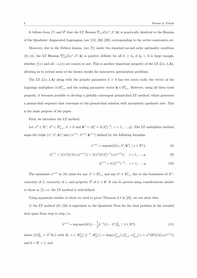
It follows from (7) and 30 that the LT Hessian ∇xxL(x∗, λ∗,k) is practically identical to the Hessian

of the Quadratic Augmented Lagrangian (see [12], [26]–[28]) corresponding to the active constraints set.

Moreover, due to the Debreu lemma, (see [7]) under the standard second order optimality condition

(3)–(4), the LT Hessian ∇2xxL(x∗, λ∗,k) is positive definite for all k ≥ k0 if k0 > 0 is large enough,

whether f(x) and all −ci(x) are convex or not. This is another important property of the LT L(x, λ,k),

allowing us to extend some of the known results for nonconvex optimization problems.

The LT L(x, λ,k) along with the penalty parameter k > 0 has two extra tools: the vector of the

Lagrange multipliers λ∈Rq++ and the scaling parameter vector k ∈ Rq

++. However, using all three tools

properly, it becomes possible to develop a globally convergent primal-dual LT method, which generates

a primal-dual sequence that converges to the primal-dual solution with asymptotic quadratic rate. This

is the main purpose of the paper.

First, we introduce the LT method.

Let x0 ∈ Rn, λ0 ∈ Rq++, k > 0 and k0 = (k0

i = k(λ0i )−2, i = 1, . . . , q). The LT multipliers method

maps the triple (xs, λs,ks) into (xs+1, λs+1,ks+1) defined by the following formulas:

xs+1 = argminL(x, λs,ks) | x ∈ Rn, (8)

λs+1i = λs

iψ′(ks

i λsi ci(x

s+1)) = λsiψ′(k(λs

i )−1ci(xs+1)), i = 1, . . . , q, (9)

ks+1i = k(λs+1

i )−2, i = 1, . . . , q. (10)

The minimizer xs+1 in (8) exists for any λs ∈ Rq++ and any ks ∈ Rq

++ due to the boundness of X∗,

convexity of f , concavity of ci and property 40 of ψ ∈ Ψ . It can be proven using considerations similar

to those in [1], i.e. the LT method is well-defined.

Using arguments similar to those we used to prove Theorem 3.1 in [25], we can show that

1) the LT method (8)–(10) is equivalent to the Quadratic Prox for the dual problem in the rescaled

dual space from step to step, i.e.

λs+1 = arg maxd(λ)− 12k−1||λ− λs||2Rs

| λ ∈ Rq, (11)

where ‖λ‖2Rs= λTRsλ with Rs = (−Ψ ′′[s](·))

−1, Ψ ′′[s](·) = diag(ψ′′[s,i](·))qi=1, ψ

′′[s,i](·) = ψ′′(θs

i ksi λ

si ci(x

s+1))

and 0 < θsi < 1, and

Primal-Dual Lagrangian Transformation method for Convex Optimization 7

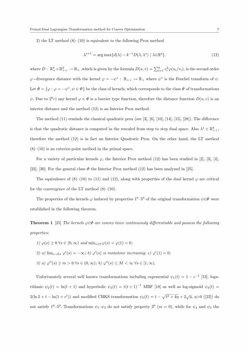
2) the LT method (8)–(10) is equivalent to the following Prox method

λs+1 = arg maxd(λ)− k−1D(λ, λs) | λ∈Rq, (12)

where D : Rq+×Rq

++ → R+ ,which is given by the formula D(u, v) =∑q

i=1 v2i ϕ(ui/vi), is the second order

ϕ−divergence distance with the kernel ϕ = −ψ∗ : R++ → R+ where ψ∗ is the Fenchel transform of ψ.

Let Φ = ϕ : ϕ = −ψ∗, ψ ∈ Ψ be the class of kernels, which corresponds to the class Ψ of transformations

ψ. Due to 20c) any kernel ϕ ∈ Φ is a barrier type function, therefore the distance function D(u, v) is an

interior distance and the method (12) is an Interior Prox method.

The method (11) reminds the classical quadratic prox (see [3], [6], [10], [14], [15], [28]). The difference

is that the quadratic distance is computed in the rescaled from step to step dual space. Also λs ∈ Rq++,

therefore the method (12) is in fact an Interior Quadratic Prox. On the other hand, the LT method

(8)–(10) is an exterior-point method in the primal space.

For a variety of particular kernels ϕ, the Interior Prox method (12) has been studied in [2], [3], [4],

[22], [30]. For the general class Φ the Interior Prox method (12) has been analyzed in [25].

The equivalence of (8)–(10) to (11) and (12), along with properties of the dual kernel ϕ are critical

for the convergence of the LT method (8)–(10).

The properties of the kernels ϕ induced by properties 10–50 of the original transformation ψ∈Ψ were

established in the following theorem.

Theorem 1 [25] The kernels ϕ∈Φ are convex twice continuously differentiable and possess the following

properties:

1) ϕ(s) ≥ 0 ∀s ∈ (0,∞) and mins≥0 ϕ(s) = ϕ(1) = 0;

2) a) lims→0+ ϕ′(s) = −∞; b) ϕ′(s) is monotone increasing; c) ϕ′(1) = 0;

3) a) ϕ′′(s) ≥ m > 0 ∀s ∈ (0,∞); b) ϕ′′(s) ≤M <∞ ∀s ∈ [1,∞).

Unfortunately several well known transformations including exponential ψ1(t) = 1 − e−t [13], loga-

rithmic ψ2(t) = ln(t + 1) and hyperbolic ψ3(t) = t(t+ 1)−1 MBF [18] as well as log-sigmoid ψ4(t) =

2(ln 2 + t − ln(1 + et)) and modified CHKS transformation ψ5(t) = t −√t2 + 4η + 2

√η, η>0 ([22]) do

not satisfy 10–50. Transformations ψ1–ψ3 do not satisfy property 30 (m = 0), while for ψ4 and ψ5 the

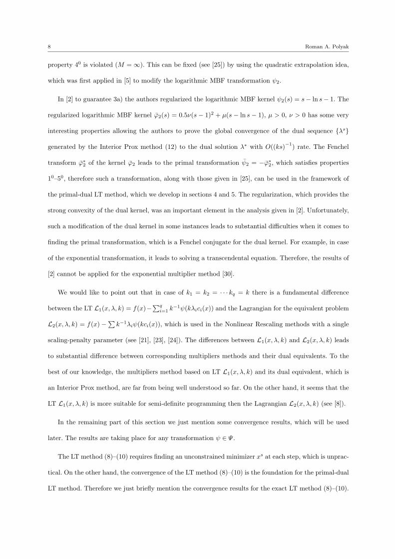
8 Roman A. Polyak

property 40 is violated (M = ∞). This can be fixed (see [25]) by using the quadratic extrapolation idea,

which was first applied in [5] to modify the logarithmic MBF transformation ψ2.

In [2] to guarantee 3a) the authors regularized the logarithmic MBF kernel ψ2(s) = s− ln s− 1. The

regularized logarithmic MBF kernel ϕ2(s) = 0.5ν(s − 1)2 + µ(s − ln s − 1), µ > 0, ν > 0 has some very

interesting properties allowing the authors to prove the global convergence of the dual sequence λs

generated by the Interior Prox method (12) to the dual solution λ∗ with O((ks)−1) rate. The Fenchel

transform ϕ∗2 of the kernel ϕ2 leads to the primal transformation ψ2 = −ϕ∗2, which satisfies properties

10–50, therefore such a transformation, along with those given in [25], can be used in the framework of

the primal-dual LT method, which we develop in sections 4 and 5. The regularization, which provides the

strong convexity of the dual kernel, was an important element in the analysis given in [2]. Unfortunately,

such a modification of the dual kernel in some instances leads to substantial difficulties when it comes to

finding the primal transformation, which is a Fenchel conjugate for the dual kernel. For example, in case

of the exponential transformation, it leads to solving a transcendental equation. Therefore, the results of

[2] cannot be applied for the exponential multiplier method [30].

We would like to point out that in case of k1 = k2 = · · · kq = k there is a fundamental difference

between the LT L1(x, λ, k) = f(x)−∑q

i=1 k−1ψ(kλici(x)) and the Lagrangian for the equivalent problem

L2(x, λ, k) = f(x) −∑k−1λiψ(kci(x)), which is used in the Nonlinear Rescaling methods with a single

scaling-penalty parameter (see [21], [23], [24]). The differences between L1(x, λ, k) and L2(x, λ, k) leads

to substantial difference between corresponding multipliers methods and their dual equivalents. To the

best of our knowledge, the multipliers method based on LT L1(x, λ, k) and its dual equivalent, which is

an Interior Prox method, are far from being well understood so far. On the other hand, it seems that the

LT L1(x, λ, k) is more suitable for semi-definite programming then the Lagrangian L2(x, λ, k) (see [8]).

In the remaining part of this section we just mention some convergence results, which will be used

later. The results are taking place for any transformation ψ ∈ Ψ .

The LT method (8)–(10) requires finding an unconstrained minimizer xs at each step, which is unprac-

tical. On the other hand, the convergence of the LT method (8)–(10) is the foundation for the primal-dual

LT method. Therefore we just briefly mention the convergence results for the exact LT method (8)–(10).

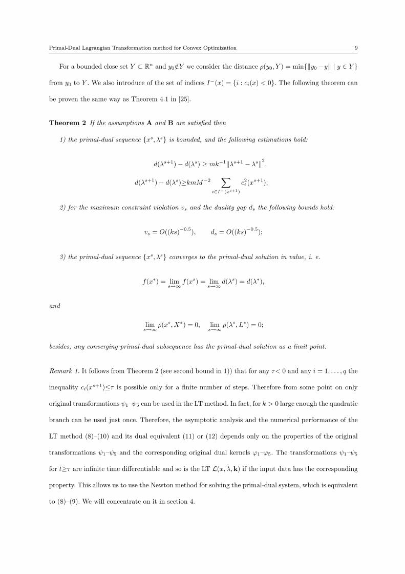
Primal-Dual Lagrangian Transformation method for Convex Optimization 9

For a bounded close set Y ⊂ Rn and y0 /∈Y we consider the distance ρ(y0, Y ) = min‖y0−y‖ | y ∈ Y

from y0 to Y . We also introduce of the set of indices I−(x) = i : ci(x) < 0. The following theorem can

be proven the same way as Theorem 4.1 in [25].

Theorem 2 If the assumptions A and B are satisfied then

1) the primal-dual sequence xs, λs is bounded, and the following estimations hold:

d(λs+1)− d(λs) ≥ mk−1‖λs+1 − λs‖2,

d(λs+1)− d(λs)≥kmM−2∑

i∈I−(xs+1)

c2i (xs+1);

2) for the maximum constraint violation vs and the duality gap ds the following bounds hold:

vs = O((ks)−0.5), ds = O((ks)−0.5);

3) the primal-dual sequence xs, λs converges to the primal-dual solution in value, i. e.

f(x∗) = lims→∞

f(xs) = lims→∞

d(λs) = d(λ∗),

and

lims→∞

ρ(xs, X∗) = 0, lims→∞

ρ(λs, L∗) = 0;

besides, any converging primal-dual subsequence has the primal-dual solution as a limit point.

Remark 1. It follows from Theorem 2 (see second bound in 1)) that for any τ< 0 and any i = 1, . . . , q the

inequality ci(xs+1)≤τ is possible only for a finite number of steps. Therefore from some point on only

original transformations ψ1–ψ5 can be used in the LT method. In fact, for k > 0 large enough the quadratic

branch can be used just once. Therefore, the asymptotic analysis and the numerical performance of the

LT method (8)–(10) and its dual equivalent (11) or (12) depends only on the properties of the original

transformations ψ1–ψ5 and the corresponding original dual kernels ϕ1–ϕ5. The transformations ψ1–ψ5

for t≥τ are infinite time differentiable and so is the LT L(x, λ,k) if the input data has the corresponding

property. This allows us to use the Newton method for solving the primal-dual system, which is equivalent

to (8)–(9). We will concentrate on it in section 4.

10 Roman A. Polyak

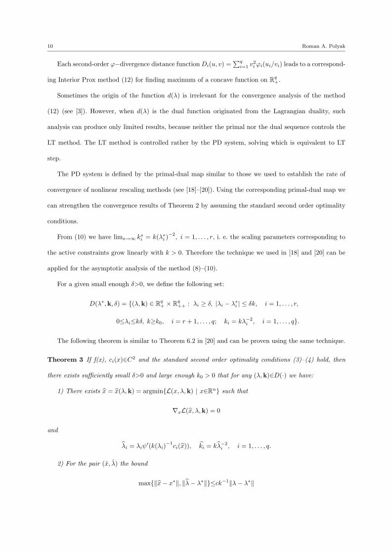
Each second-order ϕ−divergence distance functionDi(u, v) =∑q

i=1 v2i ϕi(ui/vi) leads to a correspond-

ing Interior Prox method (12) for finding maximum of a concave function on Rq+.

Sometimes the origin of the function d(λ) is irrelevant for the convergence analysis of the method

(12) (see [3]). However, when d(λ) is the dual function originated from the Lagrangian duality, such

analysis can produce only limited results, because neither the primal nor the dual sequence controls the

LT method. The LT method is controlled rather by the PD system, solving which is equivalent to LT

step.

The PD system is defined by the primal-dual map similar to those we used to establish the rate of

convergence of nonlinear rescaling methods (see [18]–[20]). Using the corresponding primal-dual map we

can strengthen the convergence results of Theorem 2 by assuming the standard second order optimality

conditions.

From (10) we have lims→∞ ksi = k(λ∗i )

−2, i = 1, . . . , r, i. e. the scaling parameters corresponding to

the active constraints grow linearly with k > 0. Therefore the technique we used in [18] and [20] can be

applied for the asymptotic analysis of the method (8)–(10).

For a given small enough δ>0, we define the following set:

D(λ∗,k, δ) = (λ,k) ∈ Rq+ × Rq

++ : λi ≥ δ, |λi − λ∗i | ≤ δk, i = 1, . . . , r,

0≤λi≤kδ, k≥k0, i = r + 1, . . . , q; ki = kλ−2i , i = 1, . . . , q.

The following theorem is similar to Theorem 6.2 in [20] and can be proven using the same technique.

Theorem 3 If f(x), ci(x)∈C2 and the standard second order optimality conditions (3)–(4) hold, then

there exists sufficiently small δ>0 and large enough k0 > 0 that for any (λ,k)∈D(·) we have:

1) There exists x = x(λ,k) = argminL(x, λ,k) | x∈Rn such that

∇xL(x, λ,k) = 0

and

λi = λiψ′(k(λi)

−1ci(x)), ki = kλ−2

i , i = 1, . . . , q.

2) For the pair (x, λ) the bound

max‖x− x∗‖, ‖λ− λ∗‖≤ck−1‖λ− λ∗‖

Primal-Dual Lagrangian Transformation method for Convex Optimization 11

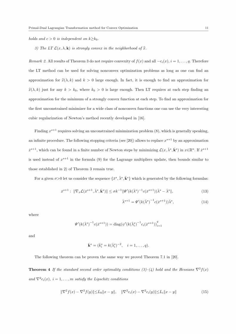
holds and c > 0 is independent on k≥k0.

3) The LT L(x, λ,k) is strongly convex in the neighborhood of x.

Remark 2. All results of Theorem 3 do not require convexity of f(x) and all −ci(x), i = 1, . . . , q. Therefore

the LT method can be used for solving nonconvex optimization problems as long as one can find an

approximation for x(λ, k) and k > 0 large enough. In fact, it is enough to find an approximation for

x(λ, k) just for any k > k0, where k0 > 0 is large enough. Then LT requires at each step finding an

approximation for the minimum of a strongly convex function at each step. To find an approximation for

the first unconstrained minimizer for a wide class of nonconvex functions one can use the very interesting

cubic regularization of Newton’s method recently developed in [16].

Finding xs+1 requires solving an unconstrained minimization problem (8), which is generally speaking,

an infinite procedure. The following stopping criteria (see [20]) allows to replace xs+1 by an approximation

xs+1, which can be found in a finite number of Newton steps by minimizing L(x, λs, ks) in x∈Rn. If xs+1

is used instead of xs+1 in the formula (9) for the Lagrange multipliers update, then bounds similar to

those established in 2) of Theorem 3 remain true.

For a given σ>0 let us consider the sequence xs, λs, ks which is generated by the following formulas:

xs+1 : ‖∇xL(xs+1, λs, ks)‖ ≤ σk−1‖Ψ ′(k(λs)−1c(xs+1))λs − λs‖, (13)

λs+1 = Ψ ′(k(λs)−1c(xs+1))λs, (14)

where

Ψ ′(k(λs)−1c(xs+1)) = diag(ψ′(k(λs

i )−1ci(xs+1))

q

i=1

and

ks = (ksi = k(λs

i )−2, i = 1, . . . , q).

The following theorem can be proven the same way we proved Theorem 7.1 in [20].

Theorem 4 If the standard second order optimality conditions (3)–(4) hold and the Hessians ∇2f(x)

and ∇2ci(x), i = 1, . . . ,m satisfy the Lipschitz conditions

‖∇2f(x)−∇2f(y)‖≤L0‖x− y‖, ‖∇2ci(x)−∇2ci(y)‖≤Li‖x− y‖ (15)

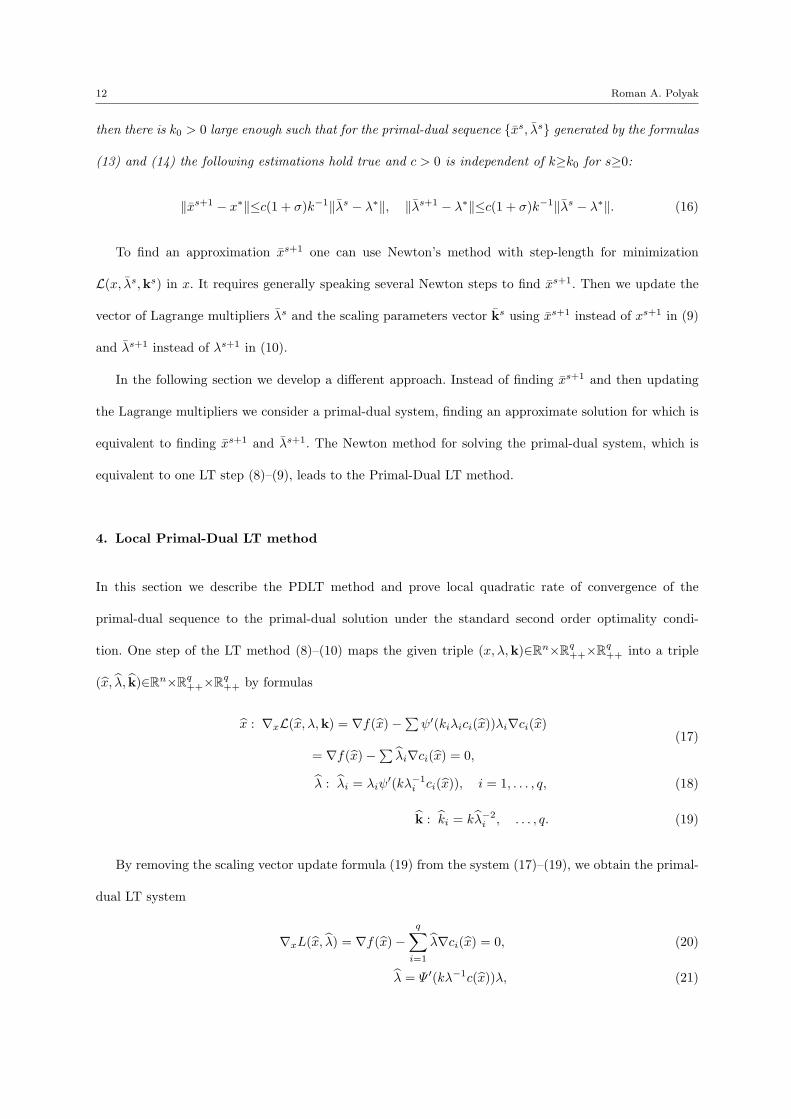
12 Roman A. Polyak

then there is k0 > 0 large enough such that for the primal-dual sequence xs, λs generated by the formulas

(13) and (14) the following estimations hold true and c > 0 is independent of k≥k0 for s≥0:

‖xs+1 − x∗‖≤c(1 + σ)k−1‖λs − λ∗‖, ‖λs+1 − λ∗‖≤c(1 + σ)k−1‖λs − λ∗‖. (16)

To find an approximation xs+1 one can use Newton’s method with step-length for minimization

L(x, λs,ks) in x. It requires generally speaking several Newton steps to find xs+1. Then we update the

vector of Lagrange multipliers λs and the scaling parameters vector ks using xs+1 instead of xs+1 in (9)

and λs+1 instead of λs+1 in (10).

In the following section we develop a different approach. Instead of finding xs+1 and then updating

the Lagrange multipliers we consider a primal-dual system, finding an approximate solution for which is

equivalent to finding xs+1 and λs+1. The Newton method for solving the primal-dual system, which is

equivalent to one LT step (8)–(9), leads to the Primal-Dual LT method.

4. Local Primal-Dual LT method

In this section we describe the PDLT method and prove local quadratic rate of convergence of the

primal-dual sequence to the primal-dual solution under the standard second order optimality condi-

tion. One step of the LT method (8)–(10) maps the given triple (x, λ,k)∈Rn×Rq++×Rq

++ into a triple

(x, λ, k)∈Rn×Rq++×Rq

++ by formulas

x : ∇xL(x, λ,k) = ∇f(x)−∑ψ′(kiλici(x))λi∇ci(x)

= ∇f(x)−∑λi∇ci(x) = 0,

(17)

λ : λi = λiψ′(kλ−1

i ci(x)), i = 1, . . . , q, (18)

k : ki = kλ−2i , . . . , q. (19)

By removing the scaling vector update formula (19) from the system (17)–(19), we obtain the primal-

dual LT system

∇xL(x, λ) = ∇f(x)−q∑

i=1

λ∇ci(x) = 0, (20)

λ = Ψ ′(kλ−1c(x))λ, (21)

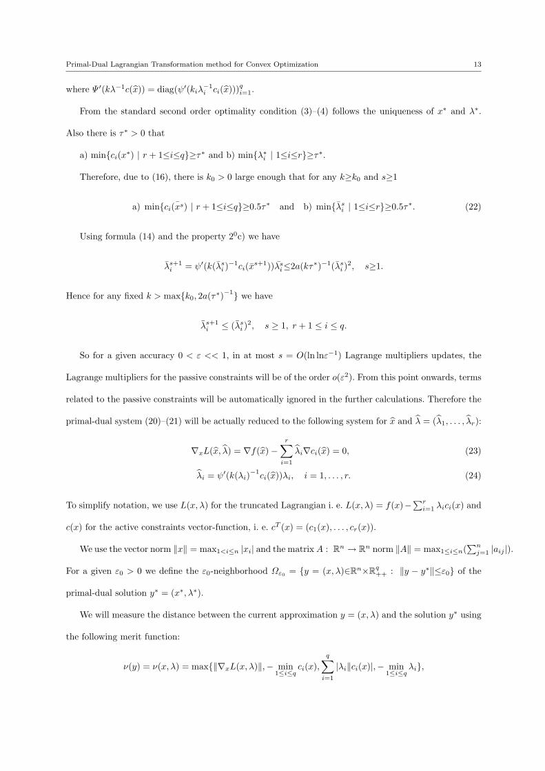
Primal-Dual Lagrangian Transformation method for Convex Optimization 13

where Ψ ′(kλ−1c(x)) = diag(ψ′(kiλ−1i ci(x)))

qi=1.

From the standard second order optimality condition (3)–(4) follows the uniqueness of x∗ and λ∗.

Also there is τ∗ > 0 that

a) minci(x∗) | r + 1≤i≤q≥τ∗ and b) minλ∗i | 1≤i≤r≥τ∗.

Therefore, due to (16), there is k0 > 0 large enough that for any k≥k0 and s≥1

a) minci ¯(xs) | r + 1≤i≤q≥0.5τ∗ and b) minλsi | 1≤i≤r≥0.5τ∗. (22)

Using formula (14) and the property 20c) we have

λs+1i = ψ′(k(λs

i )−1ci(xs+1))λs

i≤2a(kτ∗)−1(λsi )

2, s≥1.

Hence for any fixed k > maxk0, 2a(τ∗)−1 we have

λs+1i ≤ (λs

i )2, s ≥ 1, r + 1 ≤ i ≤ q.

So for a given accuracy 0 < ε << 1, in at most s = O(ln lnε−1) Lagrange multipliers updates, the

Lagrange multipliers for the passive constraints will be of the order o(ε2). From this point onwards, terms

related to the passive constraints will be automatically ignored in the further calculations. Therefore the

primal-dual system (20)–(21) will be actually reduced to the following system for x and λ = (λ1, . . . , λr):

∇xL(x, λ) = ∇f(x)−r∑

i=1

λi∇ci(x) = 0, (23)

λi = ψ′(k(λi)−1ci(x))λi, i = 1, . . . , r. (24)

To simplify notation, we use L(x, λ) for the truncated Lagrangian i. e. L(x, λ) = f(x)−∑r

i=1 λici(x) and

c(x) for the active constraints vector-function, i. e. cT (x) = (c1(x), . . . , cr(x)).

We use the vector norm ‖x‖ = max1<i≤n |xi| and the matrixA : Rn → Rn norm ‖A‖ = max1≤i≤n(∑n

j=1 |aij |).

For a given ε0 > 0 we define the ε0-neighborhood Ωε0 = y = (x, λ)∈Rn×Rq++ : ‖y − y∗‖≤ε0 of the

primal-dual solution y∗ = (x∗, λ∗).

We will measure the distance between the current approximation y = (x, λ) and the solution y∗ using

the following merit function:

ν(y) = ν(x, λ) = max‖∇xL(x, λ)‖,− min1≤i≤q

ci(x),q∑

i=1

|λi‖ci(x)|,− min1≤i≤q

λi,

14 Roman A. Polyak

assuming that the input data is properly normalized. It follows from the KKT conditions (1) and (2) that

ν(x, λ) = 0 ⇔ x = x∗, λ = λ∗.

Later we will use the following lemma.

Lemma 1. [24] If the standard second order optimality condition (3)–(4) and Lipschitz condition (15)

are satisfied, then there exists 0 < m0 < M0 <∞ and ε0 > 0 small enough that

m0‖y − y∗‖≤ν(y)≤M0‖y − y∗‖, ∀y∈Ωε0 . (25)

It follows from (25) that in the neigbourhood Ωε0 the merit function ν(y) is similar to ‖∇f(x)‖ for

the unconstrained optimization problem minf(x) | x∈Rn, when f(x) is strongly convex and ∇f(x)

satisfies the Lipschitz condition. The merit function ν(y) will be used

1) to update the penalty parameter k > 0;

2) to control accuracy at each step as well as for the overall stopping criteria;

3) to identify “small” and “large” Lagrange multipliers at each PDLT step;

4) to decide whether the primal or primal-dual direction has to be used at the current step.

First we consider the Newton method for solving system (23)– (24) and show its local quadratic

convergence. To find the Newton direction (∆x,∆λ) we have to linearize the system (23)–(24) at y =

(x, λ).

We start with system (24). Due to 30 the inverse ψ′−1 exists. Therefore, using the identity ψ′−1 = ψ∗′

and keeping in mind ϕ = −ψ∗, we can rewrite (24) as follows:

ci(x) = k−1λiψ′−1(λi/λi) = k−1λiψ

∗′(λi/λi) = −k−1λiϕ′(λi/λi).

Assuming x = x+∆x and λ = λ+∆λ, keeping in mind ϕ′(1) = 0 and ignoring terms of the second and

higher order we obtain

ci(x) = ci(x) +∇ci(x)∆x = −k−1λiϕ′((λi +∆λi)/λi)

= −k−1λiϕ′(1 +∆λi/λi) = −k−1ϕ′′(1)∆λi, i = 1, . . . , r,

or

ci(x) +∇ci(x)∆x+ k−1ϕ′′(1)∆λi = 0, i = 1, . . . , r.

Primal-Dual Lagrangian Transformation method for Convex Optimization 15

Now we linearize the system (23) at y = (x, λ). We have

∇f(x) +∇2f(x)∆x−r∑

i=1

(λi +∆λi)(∇ci(x) +∇2ci(x)∆x) = 0.

Again, ignoring terms of the second and higher orders, we obtain the following linearization of the

PD system (23)–(24):

∇2xxL(x, λ)∆x−∇cT (x)∆λ = −∇xL(x, λ), (26)

∇c(x)∆x+ k−1ϕ′′(1)Ir∆λ = −c(x), (27)

where Ir is the identical matrix in Rr and ∇c(x) = J(c(x)) is the Jacobian of the vector-function c(x).

Let us introduce the matrix

Nk(x, λ) = Nk(y) = Nk(·) =

∇2xxL(·) −∇cT (·)

∇c(·) k−1ϕ′′(1)Ir

.Then the system (26)–(27) can be written as follows:

Nk(·)

∆x∆λ

=

−∇xL(·)

−c(·)

.The local PDLT method consists of the following operations:

1. Find the primal-dual Newton direction ∆y = (∆x,∆λ) from the system

Nk(·)

∆x∆λ

=

−∇xL(·)

−c(·)

. (28)

2. Find the new primal-dual vector y = (x, λ) by formulas

x := x+∆x, λ := λ+∆λ. (29)

3. Update the scaling parameter

k = (ν(y))−1. (30)

Along with the matrix Nk(·) we consider the matrix

N∞(y) = N∞(·) =

∇2L(·) −∇cT (·)

∇c(·) 0

.We will use the following technical Lemmas later.

16 Roman A. Polyak

Lemma 2. [24] Let A : Rn→Rn be an invertible matrix and ‖A−1‖≤c0. Then for small enough ε>0 and

any B : Rn − Rn such that ‖A−B‖≤ε, the matrix B is invertible and the following bounds hold:

a) ‖B−1‖≤2c0 and b) ‖A−1 −B−1‖≤2c20ε. (31)

Lemma 3. If the standard second order optimality conditions (3)–(4) and the Lipschitz conditions (15)

are satisfied then there exists small enough ε0 > 0 and large enough k0 > 0 so that both matrices N∞(y)

and Nk(y) are non-singular and there is c0 > 0 independent of y∈Ωε0 and k≥k0 so that

max‖N−1∞ (y)‖‖N−1

k (y)‖≤2c0 ∀y∈Ωε0 and ∀k≥k0. (32)

Proof. It is well known (see Lemma 2, Chapter 8 [17]) that under the standard second order optimality

conditions (3)– (4) the matrix

N∞(x∗, λ∗) =

∇2L(x∗, λ∗) −∇cT (x∗)

∇c(x∗) 0

is non-singular, hence there exists c0 > 0 that ‖N−1

∞ (y∗)‖≤c0. Due to the Lipschitz condition (15) there

exists L > 0 that ‖Nk(y)−N∞(y∗)‖≤L‖y−y∗‖+k−1ϕ′′(1) and ‖N∞(y)−N∞(y∗)‖≤L‖y−y∗‖. Therefore

for any small enough ε > 0 there exist small ε0 > 0 and large k0 > 0 so that

max‖Nk(y)−N∞(y∗)‖, ‖N∞(y)−N∞(y∗)‖≤ε ∀y∈Ωε0 , ∀k≥k0.

Applying Lemma 2 first with A = N∞(y∗) and B = Nk(y) and then with A = N∞(y∗) and B = N∞(y)

we obtain (32).

The following theorem establishes the local quadratic convergence of the PDLT method.

Theorem 5 If the standard second order optimality conditions (3)–(4) and the Lipschitz condition (15)

are satisfied then there exists ε0 > 0 small enough that for any primal-dual pair y = (x, λ)∈Ωε0 the

PDLT methods (28)–(30) generate the primal-dual sequence that converges to the primal-dual solution

with quadratic rate, i. e. , the following bound holds:

‖y − y∗‖≤c‖y − y∗‖2 ∀y∈Ωε0 ,

and c > 0 is independent on y∈Ωε0 .

Primal-Dual Lagrangian Transformation method for Convex Optimization 17

Proof. The primal-dual Newton direction ∆y = (∆x,∆λ) we find from the system

Nk(y)∆y = b(y), (33)

where

b(y) =

−∇xL(x, λ)

−c(x)

.Along with the primal-dual system (26)–(27), we consider the Lagrange system of equations, which

corresponds to the active constraints at the same point y = (x, λ):

∇xL(x, λ) = ∇f(x)−∇c(x)Tλ=0, (34)

c(x) = 0. (35)

We apply Newton method for the system (34)–(35) from the same starting point y = (x, λ). The

Newton directions ∆y = (∆x,∆λ) for the system (34)–(35) we find from the following system of linear

equations:

N∞(y)∆y = b(y).

The new approximation for the system (34)–(35) we obtain by formulas

x = x+∆x, λ = λ+∆λ or y = y +∆y.

Under standard second order optimality conditions (3) and (4) and the Lipschitz conditions (15) there

is c1 > 0 independent on y∈Ωε0 so that the following bound holds (see Theorem 9, Ch. 8 [17]):

‖y − y∗‖≤c1‖y − y∗‖2. (36)

Now we can prove the similar bound for ‖y − y∗‖. We have

‖y − y∗‖ = ‖y +∆y − y∗‖ = ‖y +∆y +∆y −∆y − y∗‖

≤ ‖y − y∗‖+ ‖∆y −∆y‖.

For ‖∆y −∆y‖ we obtain

‖∆y −∆y‖ = ‖(N−1k (y)−N−1

∞ (y))b(y)‖ ≤ ‖N−1k (y)−N−1

∞ (y)‖‖b(y)‖.

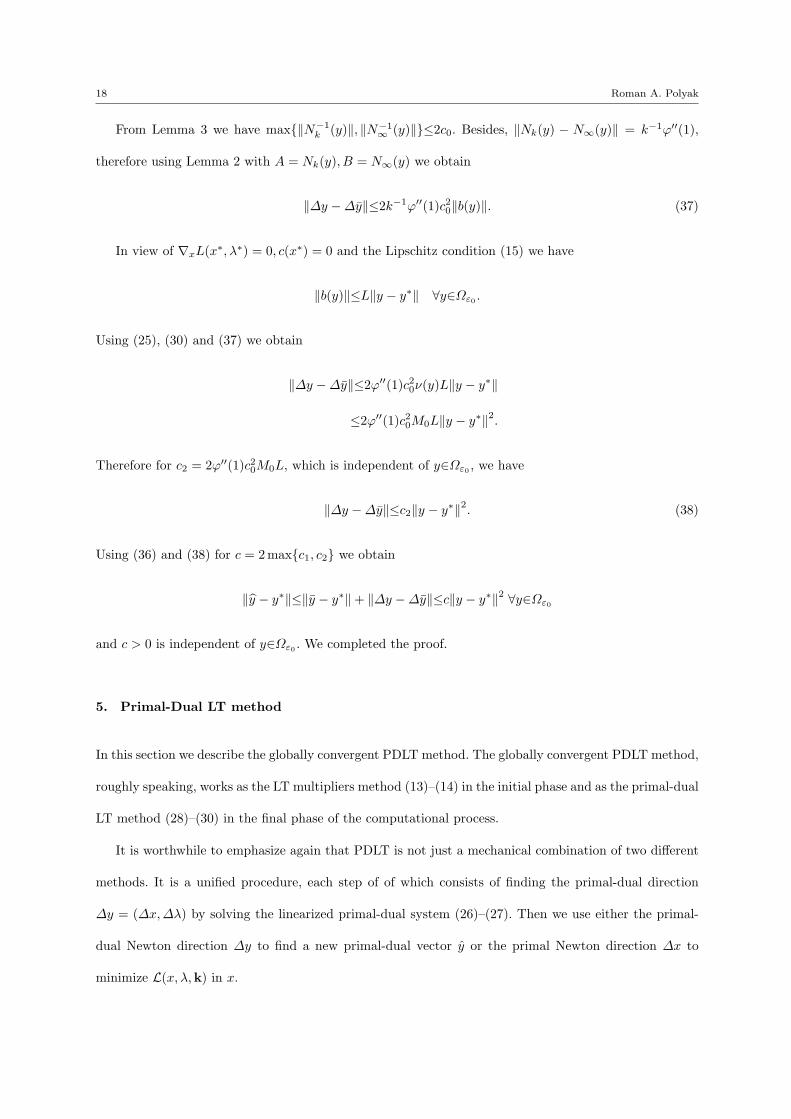
18 Roman A. Polyak

From Lemma 3 we have max‖N−1k (y)‖, ‖N−1

∞ (y)‖≤2c0. Besides, ‖Nk(y) − N∞(y)‖ = k−1ϕ′′(1),

therefore using Lemma 2 with A = Nk(y), B = N∞(y) we obtain

‖∆y −∆y‖≤2k−1ϕ′′(1)c20‖b(y)‖. (37)

In view of ∇xL(x∗, λ∗) = 0, c(x∗) = 0 and the Lipschitz condition (15) we have

‖b(y)‖≤L‖y − y∗‖ ∀y∈Ωε0 .

Using (25), (30) and (37) we obtain

‖∆y −∆y‖≤2ϕ′′(1)c20ν(y)L‖y − y∗‖

≤2ϕ′′(1)c20M0L‖y − y∗‖2.

Therefore for c2 = 2ϕ′′(1)c20M0L, which is independent of y∈Ωε0 , we have

‖∆y −∆y‖≤c2‖y − y∗‖2. (38)

Using (36) and (38) for c = 2maxc1, c2 we obtain

‖y − y∗‖≤‖y − y∗‖+ ‖∆y −∆y‖≤c‖y − y∗‖2 ∀y∈Ωε0

and c > 0 is independent of y∈Ωε0 . We completed the proof.

5. Primal-Dual LT method

In this section we describe the globally convergent PDLT method. The globally convergent PDLT method,

roughly speaking, works as the LT multipliers method (13)–(14) in the initial phase and as the primal-dual

LT method (28)–(30) in the final phase of the computational process.

It is worthwhile to emphasize again that PDLT is not just a mechanical combination of two different

methods. It is a unified procedure, each step of of which consists of finding the primal-dual direction

∆y = (∆x,∆λ) by solving the linearized primal-dual system (26)–(27). Then we use either the primal-

dual Newton direction ∆y to find a new primal-dual vector y or the primal Newton direction ∆x to

minimize L(x, λ,k) in x.

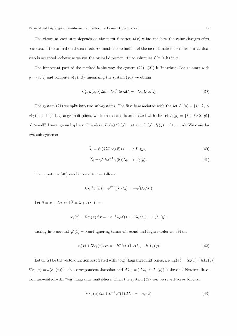
Primal-Dual Lagrangian Transformation method for Convex Optimization 19

The choice at each step depends on the merit function ν(y) value and how the value changes after

one step. If the primal-dual step produces quadratic reduction of the merit function then the primal-dual

step is accepted, otherwise we use the primal direction ∆x to minimize L(x, λ,k) in x.

The important part of the method is the way the system (20)– (21) is linearized. Let us start with

y = (x, λ) and compute ν(y). By linearizing the system (20) we obtain

∇2xxL(x, λ)∆x−∇cT (x)∆λ = −∇xL(x, λ). (39)

The system (21) we split into two sub-systems. The first is associated with the set I+(y) = i : λi >

ν(y) of “big” Lagrange multipliers, while the second is associated with the set I0(y) = i : λi≤ν(y)

of “small” Lagrange multipliers. Therefore, I+(y)∩I0(y) = ∅ and I+(y)∪I0(y) = 1, . . . , q. We consider

two sub-systems:

λi = ψ′(kλ−1i ci(x))λi, i∈I+(y), (40)

λi = ψ′(kλ−1i ci(x))λi, i∈I0(y). (41)

The equations (40) can be rewritten as follows:

kλ−1i ci(x) = ψ′

−1(λi/λi) = −ϕ′(λi/λi).

Let x = x+∆x and λ = λ+∆λ, then

ci(x) +∇ci(x)∆x = −k−1λiϕ′(1 +∆λi/λi), i∈I+(y).

Taking into account ϕ′(1) = 0 and ignoring terms of second and higher order we obtain

ci(x) +∇ci(x)∆x = −k−1ϕ′′(1)∆λi, i∈I+(y). (42)

Let c+(x) be the vector-function associated with “big” Lagrange multipliers, i. e. c+(x) = (ci(x), i∈I+(y)),

∇c+(x) = J(c+(x)) is the correspondent Jacobian and ∆λ+ = (∆λi, i∈I+(y)) is the dual Newton direc-

tion associated with “big” Lagrange multipliers. Then the system (42) can be rewritten as follows:

∇c+(x)∆x+ k−1ϕ′′(1)∆λ+ = −c+(x). (43)

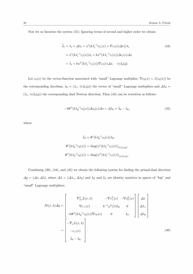
20 Roman A. Polyak

Now let us linearize the system (41). Ignoring terms of second and higher order we obtain

λi = λi +∆λi = ψ′(kλ−1i (ci(x) +∇ci(x)∆x))λi (44)

= ψ′(kλ−1i ci(x))λi + kψ′′(kλ−1

i ci(x))∆ci(x)∆x

= λi + kψ′′(kλ−1i ci(x))∇ci(x)∆x, i∈I0(y).

Let c0(x) be the vector-function associated with “small” Lagrange multiplier, ∇c0(x) = J(c0(x)) be

the corresponding Jacobian, λ0 = (λi, i∈I0(y)) the vector of “small” Lagrange multipliers and ∆λ0 =

(λi, i∈I0(y)) the corresponding dual Newton direction. Then (44) can be rewritten as follows:

−kΨ ′′(kλ−10 c0(x))∆c0(x)∆x+∆λ0 = λ0 − λ0, (45)

where

λ0 = Ψ ′(kλ−10 c0(x))λ0,

Ψ ′(kλ−10 c0(x)) = diag(ψ′(kλ−1

i ci(x)))i∈I0(y),

Ψ ′′(kλ−10 c0(x)) = diag(ψ′′(kλ−1

i ci(x)))i∈I0(y).

Combining (39), (44), and (45) we obtain the following system for finding the primal-dual direction

∆y = (∆x,∆λ), where ∆λ = (∆λ+,∆λ0) and IB and IS are identity matrices in spaces of “big” and

“small” Lagrange multipliers:

M(x, λ)∆y =

∇2

xxL(x, λ) −∇cT+(x) −∇cT0 (x)

∇c+(x) k−1ϕ′′(1)IB 0

−kΨ ′′(kλ−10 c0(x))∇c0(x) 0 IS

∆x

∆λ+

∆λ0

=

−∇xL(x, λ)

−c+(x)

λ0 − λ0

. (46)

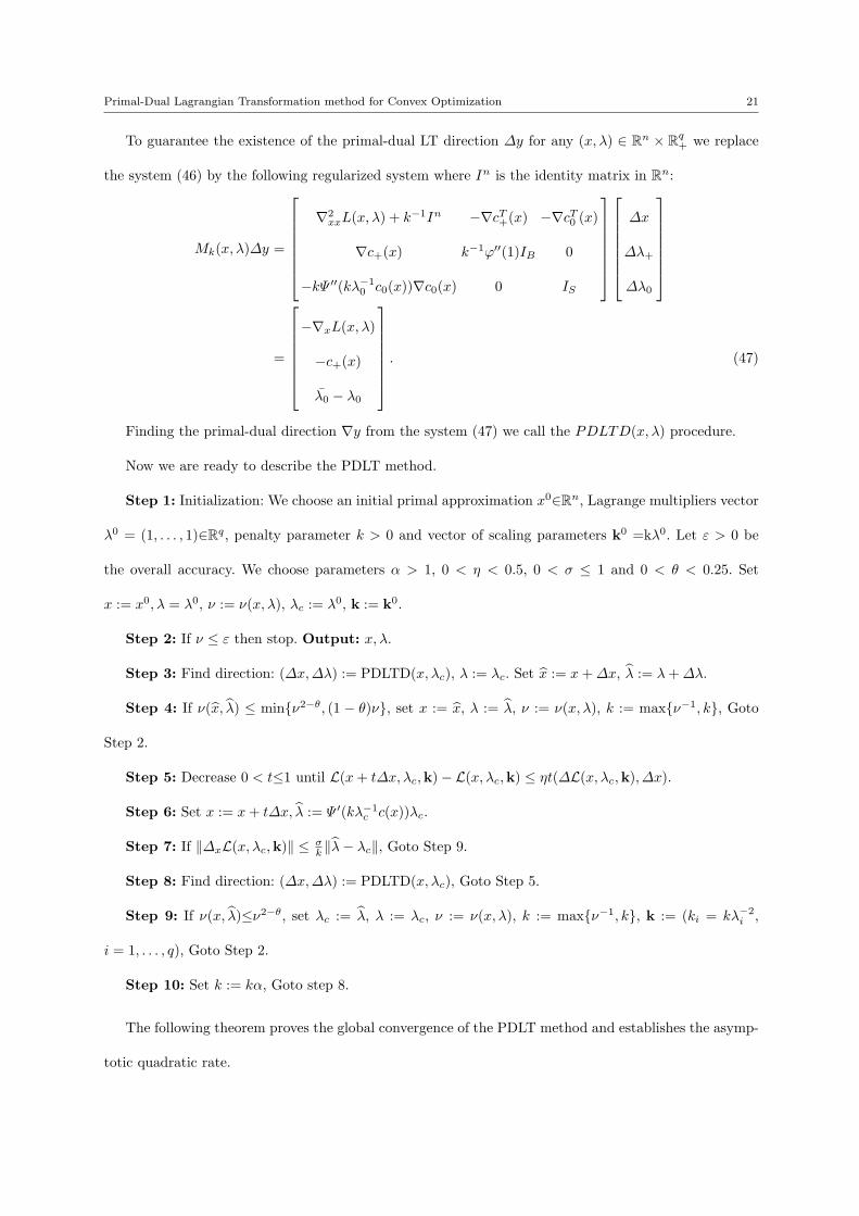
Primal-Dual Lagrangian Transformation method for Convex Optimization 21

To guarantee the existence of the primal-dual LT direction ∆y for any (x, λ) ∈ Rn × Rq+ we replace

the system (46) by the following regularized system where In is the identity matrix in Rn:

Mk(x, λ)∆y =

∇2

xxL(x, λ) + k−1In −∇cT+(x) −∇cT0 (x)

∇c+(x) k−1ϕ′′(1)IB 0

−kΨ ′′(kλ−10 c0(x))∇c0(x) 0 IS

∆x

∆λ+

∆λ0

=

−∇xL(x, λ)

−c+(x)

λ0 − λ0

. (47)

Finding the primal-dual direction ∇y from the system (47) we call the PDLTD(x, λ) procedure.

Now we are ready to describe the PDLT method.

Step 1: Initialization: We choose an initial primal approximation x0∈Rn, Lagrange multipliers vector

λ0 = (1, . . . , 1)∈Rq, penalty parameter k > 0 and vector of scaling parameters k0 =kλ0. Let ε > 0 be

the overall accuracy. We choose parameters α > 1, 0 < η < 0.5, 0 < σ ≤ 1 and 0 < θ < 0.25. Set

x := x0, λ = λ0, ν := ν(x, λ), λc := λ0, k := k0.

Step 2: If ν ≤ ε then stop. Output: x, λ.

Step 3: Find direction: (∆x,∆λ) := PDLTD(x, λc), λ := λc. Set x := x+∆x, λ := λ+∆λ.

Step 4: If ν(x, λ) ≤ minν2−θ, (1 − θ)ν, set x := x, λ := λ, ν := ν(x, λ), k := maxν−1, k, Goto

Step 2.

Step 5: Decrease 0 < t≤1 until L(x+ t∆x, λc,k)− L(x, λc,k) ≤ ηt(∆L(x, λc,k),∆x).

Step 6: Set x := x+ t∆x, λ := Ψ ′(kλ−1c c(x))λc.

Step 7: If ‖∆xL(x, λc,k)‖ ≤ σk ‖λ− λc‖, Goto Step 9.

Step 8: Find direction: (∆x,∆λ) := PDLTD(x, λc), Goto Step 5.

Step 9: If ν(x, λ)≤ν2−θ, set λc := λ, λ := λc, ν := ν(x, λ), k := maxν−1, k, k := (ki = kλ−2i ,

i = 1, . . . , q), Goto Step 2.

Step 10: Set k := kα, Goto step 8.

The following theorem proves the global convergence of the PDLT method and establishes the asymp-

totic quadratic rate.

22 Roman A. Polyak

Theorem 6 If the standard second order optimality conditions (3)–(4) and the Lipschitz condition (15)

are satisfied, then PDLT method generates a globally convergent primal-dual sequence that converges to

the primal-dual solution with asymptotic quadratic rate.

Proof. The matrix Mk(y)≡Mk(x, λ) is nonsingular for any (x, λ)∈Rn × Rq++, λ∈Rq

+ and any k > 0. Let

us consider a vector w = (u, v+, v0). Keeping in mind ψ′′(t) < 0, convexity f(x), concavity ci(x) and the

regularization term k−1In, it is easy to see that Mk(y)w = 0→w = 0. Therefore M−1k (y) exists and the

primal-dual LT direction ∆y can be found for any y = (x, λ)∈Rn×Rq+ and any k > 0.

It follows from (25) that for ∀y/∈Ωε0 there is τ>0 that ν(y)≥τ , therefore from (30) we have k−1 =

ν(y)≥τ .

After finding ∆λ+ and ∆λ0 from the second and third system in (47) and substituting their values

into the first system we obtain

Pk(y)∆x≡Pk(x, λ)∆x = −∇xL(x, λ) = −∇xL(x, λ, k), (48)

where

Pk(y) = ∇2xxL(x, λ) + k−1In

+k(ϕ′′(1))−1∇cT+(x)∇c+(x)− k∇cT0 (x)Ψ ′′(kλ−10 c0(x))∇c0(x)

and λ = (λ+, λ0), where λ+ = λ+ − k(ψ′′(1))−1c+(x), λ0 = (λi = ψ′(kλ−1

i ci(x))λi, i∈I0(y)).

Using arguments similar to those we used in case of Mk(y) we conclude that the symmetric matrix

Pk(y) is positive definite. Moreover due to k−1≥τ>0 the matrix Pk(y) has, uniformly bounded from below,

mineigenval Pk(y)≥τ > 0 ∀y/∈Ωε0 . On the other hand, for any y∈Ωε0 the mineigvalue Pk(y)≥ρ > 0

due to Debreu’s lemma [7], the standard second order optimality condition (3)–(4) and the Lipschitz

condition (15). Therefore the primal Newton direction ∆x defined by (47) or (48) is a descent direction

for minimization L(x, λ,k) in x. Therefore for 0<η≤0.5 we can find t≥t0>0 that

L(x+ t∆x, λ,k)− L(x, λ,k)≤ηt(∇xL(x, λ,k),∆x)≤− τtη‖∆x‖22. (49)

Due to the boundedness of the primal-dual sequence and the Lipschitz conditions (15) there exists

such M > 0 that ||∇xxL(x, λ,k)|| ≤ M . Hence, the primal sequence generated by Newton method

x := x+ t∆x with t > 0 defined from (49) converges to x = x(λ,k) :

Primal-Dual Lagrangian Transformation method for Convex Optimization 23

∇xL(x, λ,k) = ∇xL(x, λ) = 0.

Keeping in mind the standard second order optimality condition (3)–(4) and the Lipschitz condition

(15), it follows from Theorem 4 that for the approximation (xs+1, λs+1) the estimate (16) holds. It

requires finite number of Newton step to find xs+1. Therefore, after s0 = O(ln ε−10 ) Lagrange multipliers

and scaling parameters updates, we find the primal-dual approximation y∈Ωε0 .

Let 0 < ε << ε0 < 1 be the desired accuracy.

Keeping in mind properties 20c), 20d) of the transformation ψ∈Ψ as well as (22), (25) and (30) after

s1 = O(ln lnε−1) updates we obtain

max||kΨ ′′(kλ−10 c0(x))||, ||λ0 − λ0‖ = o(ε2), i ∈ I0. (50)

For any y∈Ωε0 the term ‖∇c0(x)‖ is bounded. The boundedness of ‖∆x‖ follows from boundedness

of ‖∇xL(x, λ)‖ and the fact that Pk(y) has a mineigenvalue bounded from below by a positive number

uniformly in y.

Let us consider the third part of the system (47), that is associated with the “small” Lagrange

multipliers

kψ′′(kλ0−1c0(x))∇c0(x)∆x+∆λ0 = λ0 − λ0.

It follows from (50) that ‖∆λ0‖ = o(ε2). This means that after s = maxs0, s1 updates the part of

the system (47) associated with “small” Lagrange multipliers becomes irrelevant for the calculation of a

Newton direction from (47). In fact, the system (47) reduces to the following system:

Mk(x, λ)∆y = b(x, λ), (51)

where ∆yT = (∆x,∆λ+), b(x, λ)T = (−∇xL(x, λ)− c+(x)), and

Mk(x, λ) =

∇2xxL(x, λ) + k−1In −∇cT(+)(x)

∇c(+)(x) k−1ϕ′′(1)IB

.At this point we have y∈Ωε0 , therefore it follows from (25) that ν(y)≤M0ε0. Hence for small enough

ε0 > 0 from |λi − λ∗i |≤ε0 we obtain λi≥ν(y), i∈I∗. On the other hand we have ν(y) > λi = O(ε2), i∈I0,

otherwise we obtain ν(y)≤O(ε2) and from (25) follows ‖y − y∗‖ = o(ε2). So, if after s = maxs0, s1

24 Roman A. Polyak

Lagrange multipliers updates we have not solved the problem with a given accuracy ε > 0 then I+(y) = I∗

and I0(y) = I∗0 = r + 1, . . . , q and we continue to perform the PDLT (28)–(30) using

Mk(y) = Mk(x, λ) =

∇2xxL(x, λ) + k−1In −∇cT(r)(x)

∇c(r)(x) k−1ϕ′′(1)Ir

instead of Nk(·) where L(x, λ) = f(x)−

∑ri=1 λici(xi).

Therefore we have

||∆y −∆y|| = ||(M−1k (y)−N−1

∞ (y))b(y)|| ≤ ||M−1k (y)−N−1

∞ (y)||||b(y)||.

On the other hand ‖Mk(y)−N∞(y)‖ ≤ k−1(1+ϕ′′(1)). From Lemma 3 we have max‖M−1k (y)‖, ‖N−1

∞ (y)‖≤2c0.

Keeping in mind (25), (30) (15) we obtain the following estimate:

‖∆y −∆y‖ ≤ 2c02k−1(1 + ϕ′′(1))‖b(y)‖ = 2c20ν(y)(1 + ϕ′′(1))‖b(y)‖

≤ 2(1 + ϕ′′(1))c20M0L‖y − y∗‖2 = c3‖y − y∗‖2, (52)

where c3 > 0 is independent of y∈S(y∗, ε0).

By using the bound (52) instead of (38) and repeating the consideration used in Theorem 5, we

conclude that the primal-dual sequence generated by PDLT converges to the primal-dual solution (x∗, λ∗)

with asymptotic quadratic rate. ut

6. Concluding remarks

The PDLT method is fundamentally different from the Newton LT multipliers method. The distinct

characteristic of the PDLT method is its global convergence with an asymptotic quadratic rate. The

PDLT method combines the best features of the Newton LT method and the Newton method for the

Lagrange system of equations corresponding to the active constraints. At the same time the PDLT method

is free from their critical drawbacks. In the initial phase the PDLT method is similar to Newton’s method

for LT minimization followed by Lagrange multipliers and scaling parameters update. Such a method (see

Theorem 4) converges under a fixed penalty parameter. This allows us to reach the ε0-neighborhood of

Primal-Dual Lagrangian Transformation method for Convex Optimization 25

the primal-dual solution in O(ln ε−10 ) Lagrange multipliers updates without compromising the condition

number of the LT Hessian.

On the other hand, once in the neighborhood of the primal-dual solution, the penalty parameter, which

is inversely proportional to the merit function, grows extremely fast. Again, the unbounded increase of

the scaling parameter at this point does not compromise the numerical stability, because instead of

uncounstrained minimization, the PDLT solves the primal-dual LT system. Moreover, the primal-dual

direction ∆y becomes very close to the Newton direction (see (52)) for the Lagrange system of equations

corresponding to the active constraints. This guarantees the asymptotic quadratic convergence.

The situation recalls the Newton method with step-length for unconstrained smooth convex optimiza-

tion.

The important part of the PDLT is the way we regularize the Hessian of the Lagrangian (see (47)).

This allows us to guarantee the global convergence, without compromising the asymptotic quadratic rate

of convergence.

Several issues remain for future research.

First, the neighborhood of the primal-dual solution where the quadratic rate of convergence occurs

needs to be characterized through parameters which measure the non-degeneracy of the constrained

optimization problems.

Second, the value of the scaling parameter k0 > 0 is a priori unknown and depends on the condition

number (see [18]) which can be expressed through parameters of a constrained optimization problem at

the solution. These parameters are obviously unknown. Therefore it is important to find an efficient way

to change the penalty parameter k > 0 using the merit function value.

Third, it is important to understand to what extent the PDLT method can be used in the non-convex

case. In this regard recent results from [16] together with local convexity properties of the LT that follow

from Debreu’s lemma [7] may play an important role.

Fourth, numerical experiments using various versions of the primal-dual NR methods produce very

encouraging results (see [11], [23] and [24]). On the other hand the PDLT method has certain specific

features that requires more numerical work to understand better its practical efficiency.

26 Roman A. Polyak

Acknowledgements. The author would like to thank Professor Kurt Anstreicher and two anonymous referees for their

remarks, which helped to improve the paper.

The research was supported by NSF Grant CCF-0324999.

References

1. A. Auslender, R. Cominetti and M. Haddou. 1997. “ Asymptotic analysis of penalty and barrier methods in convex

and linear programming. ” Math. Oper. Res. , vol. 22, pp. 43–62.

2. A. Auslender, M. Tebboule and S. Ben-Tiba. 1999. “Interior proximal and multipliers methods based on second-order

homogeneous kernels. ” Math. Oper. Res. , vol. 24, no. 3, pp. 645–668.

3. A. Auslender, M. Tebboule. 2004. “Interior Gradient and Epsilon-Subgradient Descent Methods for constrained Convex

Minimization” Math. Oper. Res. Vol 29, no1, pp1-26.

4. A. Ben-Tal and M. Zibulevsky. 1997. “Penalty-barrier methods for convex programming problems. ” SIAM J. Optim.

, vol. 7, pp. 347–366.

5. A. Ben-Tal, B. Yuzefovich and M. Zibulevsky. 1992. “Penalty-barrier multipliers methods for minimax and constrained

smooth convex optimization. ” Optimization Laboratory, Technion, Israel. Research Report 9-92.

6. D. Bertsekas. 1982. Constrained Optimization and Lagrange Multipliers Methods. Academic Press: New York.

7. G. Debreu. 1952. “Definite and Semidefinite Quadratic Forms”, Econometrica Vol. 20, P295-300.

8. M. Doljansky and M. Teboulle. 1998. “An Interior Proximal Algorithm and the Exponential Multiplier Method for

Semidefinite Programming.” SIAM J. Optim., vol. 9, no. 1, pp 1–13.

9. A. Fiacco and G. McCormick. 1990. Nonlinear Programming: Sequential Unconstrained Minimization Techniques.

Classics in Applied Mathematics. SIAM: Philadelphia, PA.

10. O. Guler. 1991. “On the convergence of the proximal point algorithm for convex minimization. ” SIAM J. Control

Optim. , vol. 29, pp. 403–419.

11. I. Griva. 2004. “Numerical experiments with an interior-exterior point method for Nonlinear Programming”. Compu-

tational Optimization and Applications, vol. 29 (2), pp. 173–195.

12. M. R. Hestenes. 1969. “Multipliers and gradient methods. ” J. Optim. Theory Appl. , vol. 4, pp. 303–320.

13. B. W. Kort and D. P. Bertsekas. 1973. “Multiplier methods for convex programming, ” in Proc. IEEE Conf. on

Decision and Control. San Diego, CA. , pp. 428–432.

14. B. Martinet. 1970. “Regularization d’inequations variationelles par approximations successive. ” Revue Francaise

d’Automatique et Informatique Rechershe Operationelle, vol. 4, pp. 154–159.

15. J. Moreau. 1965. “Proximite et dualite dans un espace Hilbertien. ” Bull. Soc. Math. France, vol. 93, pp. 273–299.

16. Y. Nesterov, B. Polyak. 2003. Cubic regularization of a Newton scheme and its global performance. Discussion paper

UCL, Center for Operations Research and Econometrics. Universite Catholique de Louvain .

17. B. Polyak, B. 1987. Introduction to Optimization. Software Inc. : NY.

18. R. Polyak. 1992. “Modified barrier functions,” Math. Programming, vol. 54, pp. 177–222.

Primal-Dual Lagrangian Transformation method for Convex Optimization 27

19. R. Polyak. 1988. “Smooth optimization methods for minmax problems,” SIAM Journal on control and optimization

vol 26 no 6, pp 1274–1286.

20. R. Polyak. 2001. “Log-sigmoid multipliers method in constrained optimization. ” Ann. Oper. Res. , vol. 101, pp.

427–460.

21. R. Polyak and M. Teboulle. 1997. “Nonlinear Rescaling and Proximal-like Methods in Convex Programming,” Math.

Programming, vol 76, pp 265–284.

22. R. Polyak. 2002. “Nonlinear rescaling vs. smoothing technique in convex optimization,” Math. Programming, vol.

92, 197–235.

23. R. Polyak and I. Griva. 2004. “Primal-dual nonlinear rescaling methods for convex optimization, ” JOTA:vol 122, No

1 pp 111-156.

24. I. Griva and R. Polyak. 2005. “Primal-Dual nonlinear rescaling method with dynamic scaling parameter update,”

Math. Programming, published online, June 7, 2005

25. R. Polyak. 2005 “Nonlinear Rescaling as Interior Quadratic Prox method for Convex Optimization” to appear in

COAP.

26. M. J. D. Powell. 1969. “A method for nonlinear constraints in minimization problems, ” in Fletcher, ed. , Optimization,

London Academic Press, pp. 283–298.

27. R. T. Rockafellar. 1973. “A dual approach to solving nonlinear programming problems by unconstrainted minimization.

” Math. Programming, vol. 5, pp. 354–373.

28. R. T. Rockafellar. 1976. “Augmented Lagrangians and applications of the proximal points algorithms in convex pro-

gramming. ” Math. Oper. Res. , vol. 1, pp. 97–116.

29. D. F. Shanno and R. J. Vanderbei. 1999. “An interior point algorithm for nonconvex nonlinear programming. ” COAP,

vol. 13, pp. 231–252.

30. P. Tseng and D. Bertsekas. 1993. “On the convergence of the exponential multipliers method for convex programming.

” Math. Programming, vol. 60, pp. 1–19.