Convex Hulls, Voronoi Diagrams and Delaunay Triangulations · 2010-01-12 · Convex hull P conv(P)...
98
Convex Hulls, Voronoi Diagrams and Delaunay Triangulations Jean-Daniel Boissonnat Winter School on Algorithmic Geometry ENS-Lyon January 2010 Winter School on Algorithmic Geometry Convex Hulls, Voronoi Diagrams and Delaunay Triangulations
Transcript of Convex Hulls, Voronoi Diagrams and Delaunay Triangulations · 2010-01-12 · Convex hull P conv(P)...
Convex Hulls, Voronoi Diagrams andDelaunay Triangulations
Jean-Daniel Boissonnat
Winter School on Algorithmic GeometryENS-Lyon
January 2010
Winter School on Algorithmic Geometry Convex Hulls, Voronoi Diagrams and Delaunay Triangulations
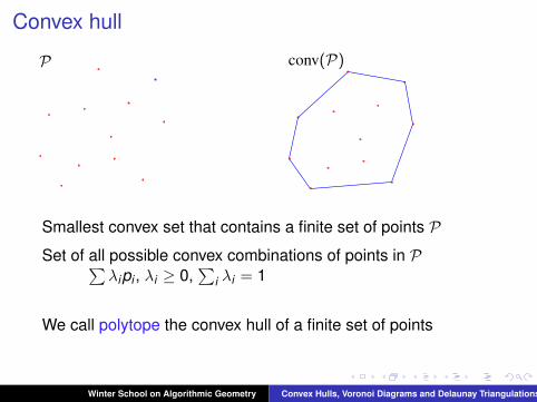
Convex hull
P conv(P)
Smallest convex set that contains a finite set of points PSet of all possible convex combinations of points in P∑
λipi , λi ≥ 0,∑
i λi = 1
We call polytope the convex hull of a finite set of points
Winter School on Algorithmic Geometry Convex Hulls, Voronoi Diagrams and Delaunay Triangulations
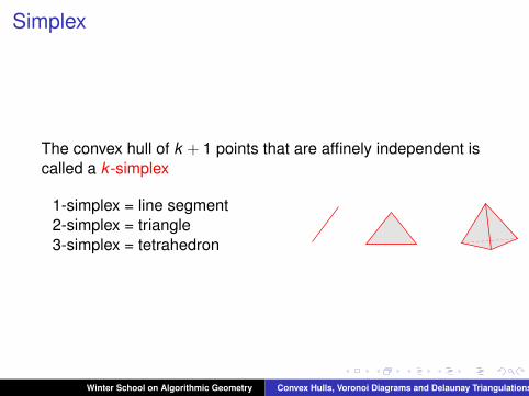
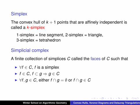
Simplex
The convex hull of k + 1 points that are affinely independent iscalled a k -simplex
1-simplex = line segment2-simplex = triangle3-simplex = tetrahedron
Winter School on Algorithmic Geometry Convex Hulls, Voronoi Diagrams and Delaunay Triangulations
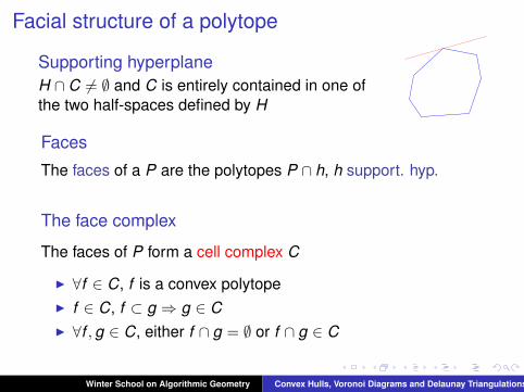
Facial structure of a polytope
Supporting hyperplaneH ∩ C 6= ∅ and C is entirely contained in one ofthe two half-spaces defined by H
Faces
The faces of a P are the polytopes P ∩ h, h support. hyp.
The face complex
The faces of P form a cell complex C
I ∀f ∈ C, f is a convex polytopeI f ∈ C, f ⊂ g ⇒ g ∈ CI ∀f ,g ∈ C, either f ∩ g = ∅ or f ∩ g ∈ C
Winter School on Algorithmic Geometry Convex Hulls, Voronoi Diagrams and Delaunay Triangulations
General position
A point set P is said to be in general position iff no subset ofk + 2 points lie in a k -flat
If P is in general position, all the faces of conv(P) are simplices
The boundary of conv(P) is a simplicial complex
Winter School on Algorithmic Geometry Convex Hulls, Voronoi Diagrams and Delaunay Triangulations
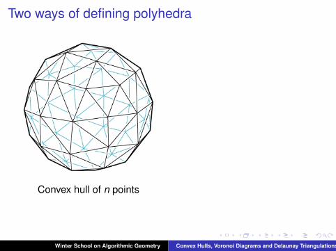
Two ways of defining polyhedra
Convex hull of n points
Intersection of n half-spaces
Winter School on Algorithmic Geometry Convex Hulls, Voronoi Diagrams and Delaunay Triangulations
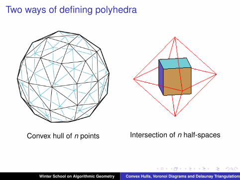
Two ways of defining polyhedra
Convex hull of n points Intersection of n half-spaces
Winter School on Algorithmic Geometry Convex Hulls, Voronoi Diagrams and Delaunay Triangulations
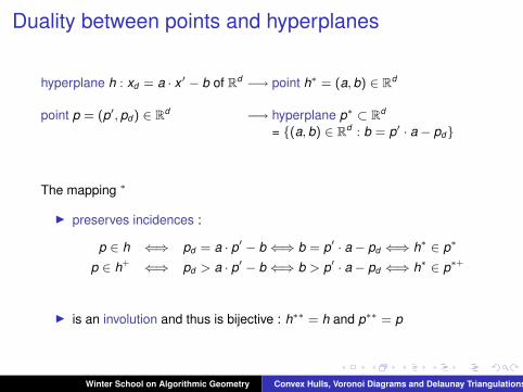
Duality between points and hyperplanes
hyperplane h : xd = a · x ′ − b of Rd −→ point h∗ = (a, b) ∈ Rd
point p = (p′, pd) ∈ Rd −→ hyperplane p∗ ⊂ Rd
= {(a, b) ∈ Rd : b = p′ · a− pd}
The mapping ∗
I preserves incidences :
p ∈ h ⇐⇒ pd = a · p′ − b ⇐⇒ b = p′ · a− pd ⇐⇒ h∗ ∈ p∗
p ∈ h+ ⇐⇒ pd > a · p′ − b ⇐⇒ b > p′ · a− pd ⇐⇒ h∗ ∈ p∗+
I is an involution and thus is bijective : h∗∗ = h and p∗∗ = p
Winter School on Algorithmic Geometry Convex Hulls, Voronoi Diagrams and Delaunay Triangulations
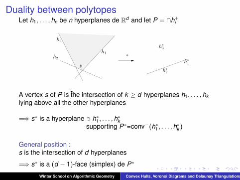
Duality between polytopesLet h1, . . . ,hn be n hyperplanes de Rd and let P = ∩h+
i
ss
h1h2 *
h3
h∗3
h∗2
h∗1
A vertex s of P is the intersection of k ≥ d hyperplanes h1, . . . ,hklying above all the other hyperplanes
=⇒ s∗ is a hyperplane 3 h∗1 , . . . ,h∗k
supporting P∗=conv−(h∗1 , . . . ,h∗k )
General position :s is the intersection of d hyperplanes
=⇒ s∗ is a (d − 1)-face (simplex) de P∗
Winter School on Algorithmic Geometry Convex Hulls, Voronoi Diagrams and Delaunay Triangulations
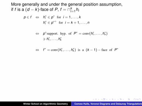
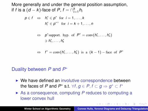
More generally and under the general position assumption,if f is a (d − k)-face of P, f = ∩k
i=1hi
p ∈ f ⇔ h∗i ∈ p∗ for i = 1, . . . , k
h∗i ∈ p∗+ for i = k + 1, . . . , n
⇔ p∗support. hyp. of P∗ = conv(h∗1 , . . . , h∗n )
3 h∗1 , . . . , h∗k
⇔ f ∗ = conv(h∗1 , . . . , h∗k ) is a (k − 1)− face of P∗
Duality between P and P∗
I We have defined an involutive correspondence betweenthe faces of P and P∗ s.t. ∀f ,g ∈ P, f ⊂ g ⇒ g∗ ⊂ f ∗
I As a consequence, computing P reduces to computing alower convex hull
Winter School on Algorithmic Geometry Convex Hulls, Voronoi Diagrams and Delaunay Triangulations
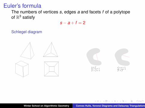
Euler’s formulaThe numbers of vertices s, edges a and facets f of a polytopeof R3 satisfy
s − a + f = 2
Schlegel diagram
s = s′a′ = a + 1f ′ = f + 1
a′ = a + 1f ′ = f
s′ = s + 1
Winter School on Algorithmic Geometry Convex Hulls, Voronoi Diagrams and Delaunay Triangulations
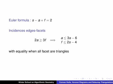
Euler formula : s − a + f = 2
Incidences edges-facets
2a ≥ 3f =⇒ a ≤ 3s − 6f ≤ 2s − 4
with equality when all facet are triangles
Winter School on Algorithmic Geometry Convex Hulls, Voronoi Diagrams and Delaunay Triangulations
Beyond the 3rd dimensionUpper bound theorem [McMullen 1970]
If P is the intersection of n half-spaces of Rd
nb faces of P = Θ(nb d2 c)
General position
all vertices of P are incident to d edges (in the worst-case) andhave distinct xd
⇒ the convex hull of k < d edges incident to a vertex p is ak -face of P
⇒ any k -face is the intersection of d − k hyperplanes definingP
Winter School on Algorithmic Geometry Convex Hulls, Voronoi Diagrams and Delaunay Triangulations

Proof of the upper bound th.
1. ≥ dd2 e edges incident to a vertex p are in h+
p : xd ≥ xd (p)or in h−p⇒ p is a xd -max or xd -min vertex of at least one d d
2 e-face of P⇒ # vertices of P ≤ 2×# d d
2 e-faces of P
2. A k -face is the intersection of d − k hyperplanes defining P
⇒ # k -faces =
(n
d − k
)= O(nd−k )
⇒ # d d2 e-faces = O(nb
d2 c)
3. The number of faces incident to p depends on d but not onn
Winter School on Algorithmic Geometry Convex Hulls, Voronoi Diagrams and Delaunay Triangulations
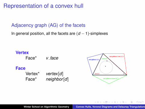
Representation of a convex hull
Adjacency graph (AG) of the facets
In general position, all the facets are (d − 1)-simplexes
VertexFace* v face
FaceVertex* vertex [d ]Face* neighbor [d ]
i
f
neighbor(ccw(i))
cw(i)
neighbor(i) ccw(i)neighbor(cw(i))
Winter School on Algorithmic Geometry Convex Hulls, Voronoi Diagrams and Delaunay Triangulations
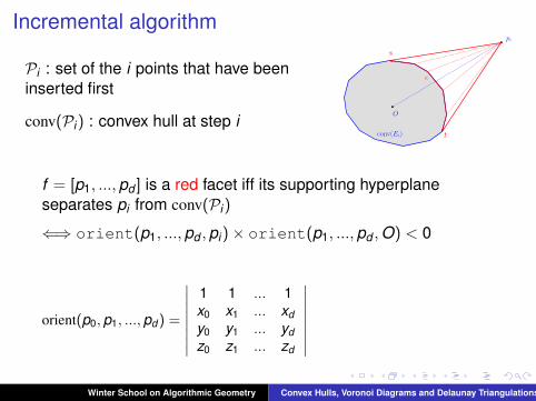
Incremental algorithm
Pi : set of the i points that have beeninserted first
conv(Pi) : convex hull at step iO
pi
conv(Ei)
e
s
t
f = [p1, ...,pd ] is a red facet iff its supporting hyperplaneseparates pi from conv(Pi)
⇐⇒ orient(p1, ...,pd ,pi)× orient(p1, ...,pd ,O) < 0
orient(p0,p1, ...,pd ) =
∣∣∣∣∣∣∣∣1 1 ... 1x0 x1 ... xdy0 y1 ... ydz0 z1 ... zd
∣∣∣∣∣∣∣∣Winter School on Algorithmic Geometry Convex Hulls, Voronoi Diagrams and Delaunay Triangulations
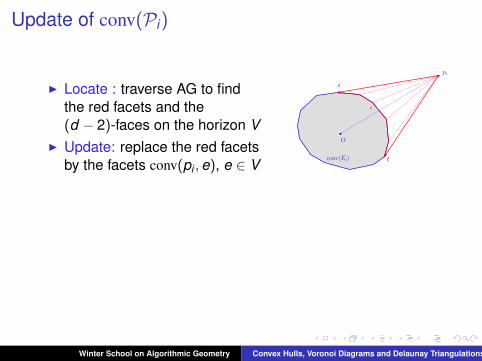
Update of conv(Pi)
I Locate : traverse AG to findthe red facets and the(d − 2)-faces on the horizon V
I Update: replace the red facetsby the facets conv(pi ,e), e ∈ V
O
pi
conv(Ei)
e
s
t
Correctness
I The AG of the red facets is connectedI The new faces are all obtained as above
Winter School on Algorithmic Geometry Convex Hulls, Voronoi Diagrams and Delaunay Triangulations
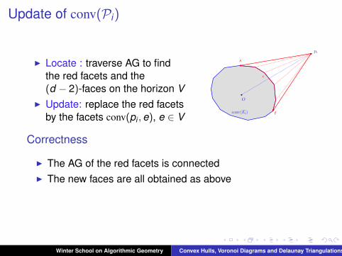
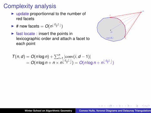
Complexity analysisI update proportionnal to the number of
red facets
I # new facets = O(nbd−1
2 c)
I fast locate : insert the points inlexicographic order and attach a facet toeach point
O
pi
conv(Ei)
e
s
t
T (n,d) = O(n log n) +∑n
i=1 |conv(i ,d − 1)|= O(n log n + n × nb d−1
2 c) = O(n log n + nb d+12 c)
Optimal in even dimensions
Can be improved to O(n log n) when d = 3
The expected complexity can be improved to O(n log n + nb d2 c) by
inserting the points in random order (see course 3)
The randomized algorithm can be derandomized [Chazelle 1992]
Winter School on Algorithmic Geometry Convex Hulls, Voronoi Diagrams and Delaunay Triangulations
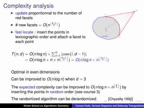
Complexity analysisI update proportionnal to the number of
red facets
I # new facets = O(nbd−1
2 c)
I fast locate : insert the points inlexicographic order and attach a facet toeach point
O
pi
conv(Ei)
e
s
t
T (n,d) = O(n log n) +∑n
i=1 |conv(i ,d − 1)|= O(n log n + n × nb d−1
2 c) = O(n log n + nb d+12 c)
Optimal in even dimensions
Can be improved to O(n log n) when d = 3
The expected complexity can be improved to O(n log n + nb d2 c) by
inserting the points in random order (see course 3)
The randomized algorithm can be derandomized [Chazelle 1992]
Winter School on Algorithmic Geometry Convex Hulls, Voronoi Diagrams and Delaunay Triangulations
Delaunay Triangulations
Winter School on Algorithmic Geometry Convex Hulls, Voronoi Diagrams and Delaunay Triangulations
Simplex
The convex hull of k + 1 points that are affinely independent iscalled a k -simplex
1-simplex = line segment, 2-simplex = triangle,3-simplex = tetrahedron
Simplicial complex
A finite collection of simplices C called the faces of C such that
I ∀f ∈ C, f is a simplexI f ∈ C, f ⊂ g ⇒ g ∈ CI ∀f ,g ∈ C, either f ∩ g = ∅ or f ∩ g ∈ C
Winter School on Algorithmic Geometry Convex Hulls, Voronoi Diagrams and Delaunay Triangulations
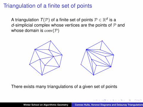
Triangulation of a finite set of points
A triangulation T (P) of a finite set of points P ∈ Rd is ad-simplicial complex whose vertices are the points of P andwhose domain is conv(P)
There exists many triangulations of a given set of points
Winter School on Algorithmic Geometry Convex Hulls, Voronoi Diagrams and Delaunay Triangulations
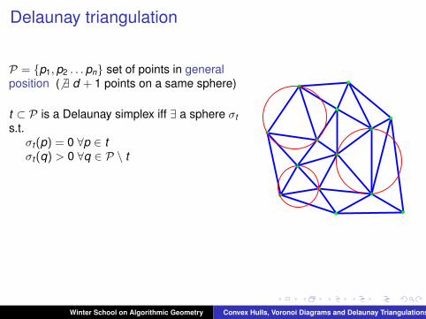
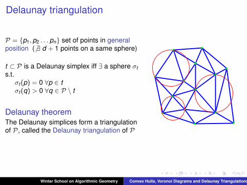
Delaunay triangulation
P = {p1,p2 . . . pn} set of points in generalposition (6 ∃ d + 1 points on a same sphere)
t ⊂ P is a Delaunay simplex iff ∃ a sphere σts.t.
σt (p) = 0 ∀p ∈ tσt (q) > 0 ∀q ∈ P \ t
Delaunay theoremThe Delaunay simplices form a triangulationof P, called the Delaunay triangulation of P
Winter School on Algorithmic Geometry Convex Hulls, Voronoi Diagrams and Delaunay Triangulations
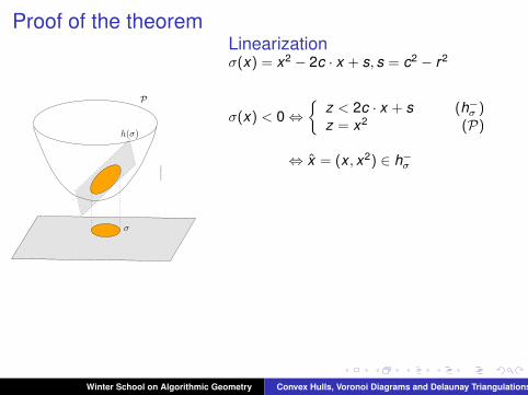
Proof of the theorem
σ
h(σ)
P
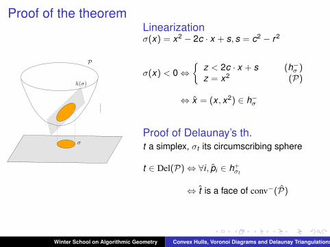
Linearizationσ(x) = x2 − 2c · x + s, s = c2 − r2
σ(x) < 0⇔{
z < 2c · x + s (h−σ )z = x2 (P)
⇔ x = (x , x2) ∈ h−σ
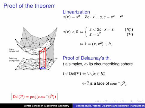
Proof of Delaunay’s th.t a simplex, σt its circumscribing sphere
t ∈ Del(P)⇔ ∀i , pi ∈ h+σt
⇔ t is a face of conv−(P)
Del(P) = proj(conv−(P))
Winter School on Algorithmic Geometry Convex Hulls, Voronoi Diagrams and Delaunay Triangulations
Proof of the theorem
σ
h(σ)
P
Linearizationσ(x) = x2 − 2c · x + s, s = c2 − r2
σ(x) < 0⇔{
z < 2c · x + s (h−σ )z = x2 (P)
⇔ x = (x , x2) ∈ h−σ
Proof of Delaunay’s th.t a simplex, σt its circumscribing sphere
t ∈ Del(P)⇔ ∀i , pi ∈ h+σt
⇔ t is a face of conv−(P)
Del(P) = proj(conv−(P))
Winter School on Algorithmic Geometry Convex Hulls, Voronoi Diagrams and Delaunay Triangulations
Proof of the theoremLinearizationσ(x) = x2 − 2c · x + s, s = c2 − r2
σ(x) < 0⇔{
z < 2c · x + s (h−σ )z = x2 (P)
⇔ x = (x , x2) ∈ h−σ
Proof of Delaunay’s th.t a simplex, σt its circumscribing sphere
t ∈ Del(P)⇔ ∀i , pi ∈ h+σt
⇔ t is a face of conv−(P)
Del(P) = proj(conv−(P))
Winter School on Algorithmic Geometry Convex Hulls, Voronoi Diagrams and Delaunay Triangulations
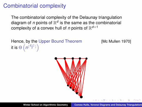
Combinatorial complexity
The combinatorial complexity of the Delaunay triangulationdiagram of n points of Rd is the same as the combinatorialcomplexity of a convex hull of n points of Rd+1
Hence, by the Upper Bound Theorem [Mc Mullen 1970]
it is Θ(
nbd+1
2 c)
Winter School on Algorithmic Geometry Convex Hulls, Voronoi Diagrams and Delaunay Triangulations
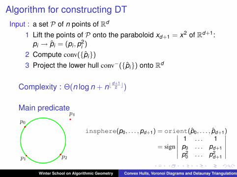
Algorithm for constructing DTInput : a set P of n points of Rd
1 Lift the points of P onto the paraboloid xd+1 = x2 of Rd+1:pi → pi = (pi ,p2
i )
2 Compute conv({pi})3 Project the lower hull conv−({pi}) onto Rd
Complexity : Θ(n log n + nbd+1
2 c)
Main predicate
p0
p1p2
p4
insphere(p0, . . . ,pd+1) = orient(p0, . . . , pd+1)
= sign
∣∣∣∣∣∣1 . . . 1p0 . . . pd+1p2
0 . . . p2d+1
∣∣∣∣∣∣Winter School on Algorithmic Geometry Convex Hulls, Voronoi Diagrams and Delaunay Triangulations
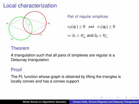
Local characterization
fq1 q2
σ1
σ2
Pair of regular simplices
σ2(q1) ≥ 0 and σ1(q2) ≥ 0
⇔ c1 ∈ h+σ2
and c2 ∈ h+σ1
TheoremA triangulation such that all pairs of simplexes are regular is aDelaunay triangulation
ProofThe PL function whose graph is obtained by lifting the triangles islocally convex and has a convex support
Winter School on Algorithmic Geometry Convex Hulls, Voronoi Diagrams and Delaunay Triangulations
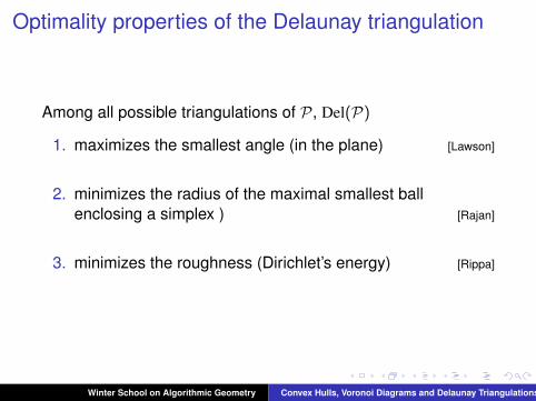
Optimality properties of the Delaunay triangulation
Among all possible triangulations of P, Del(P)
1. maximizes the smallest angle (in the plane) [Lawson]
2. minimizes the radius of the maximal smallest ballenclosing a simplex ) [Rajan]
3. minimizes the roughness (Dirichlet’s energy) [Rippa]
Winter School on Algorithmic Geometry Convex Hulls, Voronoi Diagrams and Delaunay Triangulations
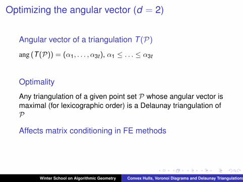
Optimizing the angular vector (d = 2)
Angular vector of a triangulation T (P)
ang (T (P)) = (α1, . . . , α3t ), α1 ≤ . . . ≤ α3t
Optimality
Any triangulation of a given point set P whose angular vector ismaximal (for lexicographic order) is a Delaunay triangulation ofP
Affects matrix conditioning in FE methods
Winter School on Algorithmic Geometry Convex Hulls, Voronoi Diagrams and Delaunay Triangulations
Constructive proof using flips
a
b
c
d
a
b
d
c
t3
t4
a4
c4d4
a3
b3
d3
a1
t1
c1
b1
c2
d2
t2
b2
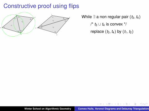
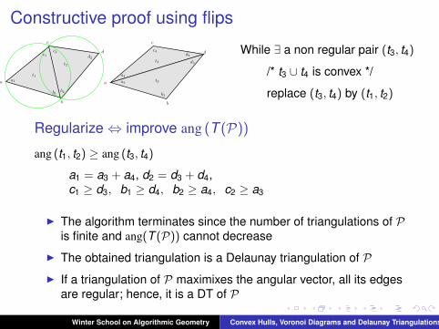
While ∃ a non regular pair (t3, t4)
/* t3 ∪ t4 is convex */
replace (t3, t4) by (t1, t2)
Regularize⇔ improve ang (T (P))
ang (t1, t2) ≥ ang (t3, t4)
a1 = a3 + a4, d2 = d3 + d4,c1 ≥ d3, b1 ≥ d4, b2 ≥ a4, c2 ≥ a3
I The algorithm terminates since the number of triangulations of Pis finite and ang(T (P)) cannot decrease
I The obtained triangulation is a Delaunay triangulation of PI If a triangulation of P maximixes the angular vector, all its edges
are regular; hence, it is a DT of P
Winter School on Algorithmic Geometry Convex Hulls, Voronoi Diagrams and Delaunay Triangulations
Constructive proof using flips
a
b
c
d
a
b
d
c
t3
t4
a4
c4d4
a3
b3
d3
a1
t1
c1
b1
c2
d2
t2
b2
While ∃ a non regular pair (t3, t4)
/* t3 ∪ t4 is convex */
replace (t3, t4) by (t1, t2)
Regularize⇔ improve ang (T (P))
ang (t1, t2) ≥ ang (t3, t4)
a1 = a3 + a4, d2 = d3 + d4,c1 ≥ d3, b1 ≥ d4, b2 ≥ a4, c2 ≥ a3
I The algorithm terminates since the number of triangulations of Pis finite and ang(T (P)) cannot decrease
I The obtained triangulation is a Delaunay triangulation of PI If a triangulation of P maximixes the angular vector, all its edges
are regular; hence, it is a DT of P
Winter School on Algorithmic Geometry Convex Hulls, Voronoi Diagrams and Delaunay Triangulations
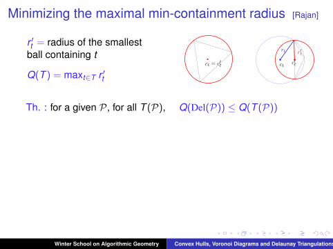
Minimizing the maximal min-containment radius [Rajan]
r ′t = radius of the smallestball containing t
Q(T ) = maxt∈T r ′t
ct = c′t ct c′t
rt r′t
Th. : for a given P, for all T (P), Q(Del(P)) ≤ Q(T (P))
Interpolation error [Waldron 98]
If g is the linear interpolation of f over a simplex t ,
‖f − g‖∞ ≤ ctr′2t2
ct = bound on the absolute curvature of f in t
Winter School on Algorithmic Geometry Convex Hulls, Voronoi Diagrams and Delaunay Triangulations
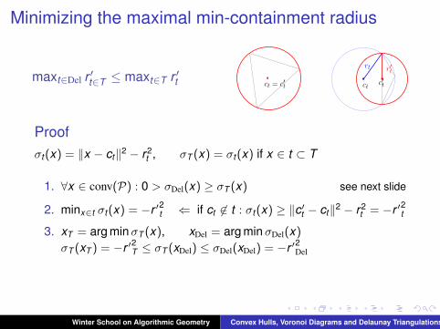
Minimizing the maximal min-containment radius
maxt∈Del r ′t∈T ≤ maxt∈T r ′t ct = c′t ct c′t
rt r′t
Proofσt (x) = ‖x − ct‖2 − r2
t , σT (x) = σt (x) if x ∈ t ⊂ T
1. ∀x ∈ conv(P) : 0 > σDel(x) ≥ σT (x) see next slide
2. minx∈t σt (x) = −r ′2t ⇐ if ct 6∈ t : σt (x) ≥ ‖c′t − ct‖2 − r2t = −r ′2t
3. xT = arg minσT (x), xDel = arg minσDel(x)
σT (xT ) = −r ′2T ≤ σT (xDel) ≤ σDel(xDel) = −r ′2Del
Winter School on Algorithmic Geometry Convex Hulls, Voronoi Diagrams and Delaunay Triangulations

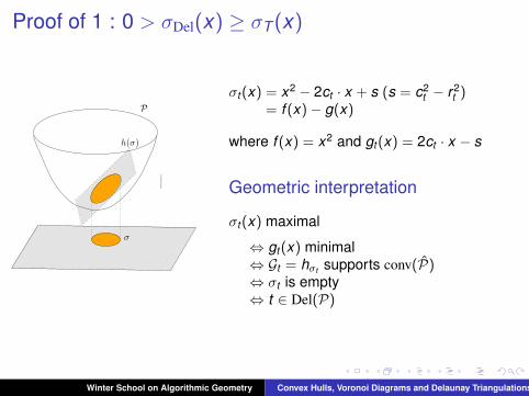
Proof of 1 : 0 > σDel(x) ≥ σT (x)
σ
h(σ)
Pσt (x) = x2 − 2ct · x + s (s = c2
t − r2t )
= f (x)− g(x)
where f (x) = x2 and gt (x) = 2ct · x − s
Geometric interpretation
σt (x) maximal
⇔ gt (x) minimal⇔ Gt = hσt supports conv(P)⇔ σt is empty⇔ t ∈ Del(P)
Winter School on Algorithmic Geometry Convex Hulls, Voronoi Diagrams and Delaunay Triangulations
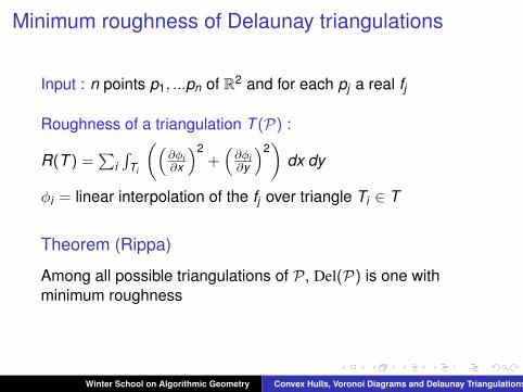
Minimum roughness of Delaunay triangulations
Input : n points p1, ...pn of R2 and for each pj a real fj
Roughness of a triangulation T (P) :
R(T ) =∑
i∫
Ti
((∂φi∂x
)2+(∂φi∂y
)2)
dx dy
φi = linear interpolation of the fj over triangle Ti ∈ T
Theorem (Rippa)
Among all possible triangulations of P, Del(P) is one withminimum roughness
Winter School on Algorithmic Geometry Convex Hulls, Voronoi Diagrams and Delaunay Triangulations
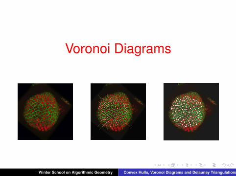
Voronoi Diagrams
Winter School on Algorithmic Geometry Convex Hulls, Voronoi Diagrams and Delaunay Triangulations
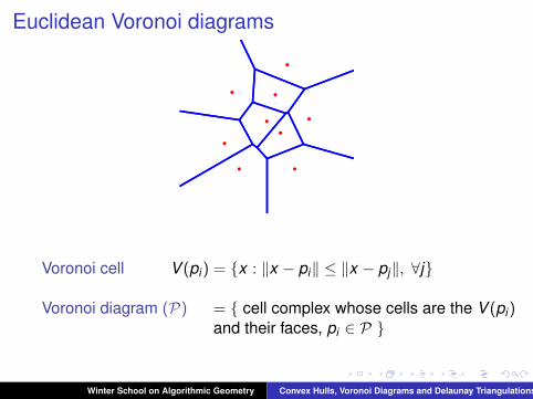
Euclidean Voronoi diagrams
Voronoi cell V (pi) = {x : ‖x − pi‖ ≤ ‖x − pj‖, ∀j}
Voronoi diagram (P) = { cell complex whose cells are the V (pi)and their faces, pi ∈ P }
Winter School on Algorithmic Geometry Convex Hulls, Voronoi Diagrams and Delaunay Triangulations
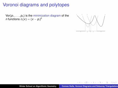
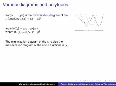
Voronoi diagrams and polytopes
Vor(p1, . . . , pn) is the minimization diagram of then functions δi(x) = (x − pi)
2
arg min(δi) = arg max(hi)where hpi (x) = 2 pi · x − p2
i
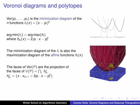
The minimization diagram of the δi is also themaximization diagram of the affine functions hi(x)
The faces of Vor(P) are the projection ofthe faces of V(P) =
Ti h+
pi
h+pi
= {x : xd+1 > 2pi · x − p2i }
1 2 3 4
1 2 1 3 4
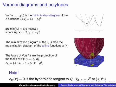
Note !
hpi (x) = 0 is the hyperplane tangent to Q : xd+1 = x2 at (x , x2)
Winter School on Algorithmic Geometry Convex Hulls, Voronoi Diagrams and Delaunay Triangulations
Voronoi diagrams and polytopes
Vor(p1, . . . , pn) is the minimization diagram of then functions δi(x) = (x − pi)
2
arg min(δi) = arg max(hi)where hpi (x) = 2 pi · x − p2
i
The minimization diagram of the δi is also themaximization diagram of the affine functions hi(x)
The faces of Vor(P) are the projection ofthe faces of V(P) =
Ti h+
pi
h+pi
= {x : xd+1 > 2pi · x − p2i }
1 2 3 4
1 2 1 3 4
Note !
hpi (x) = 0 is the hyperplane tangent to Q : xd+1 = x2 at (x , x2)
Winter School on Algorithmic Geometry Convex Hulls, Voronoi Diagrams and Delaunay Triangulations
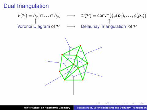
Dual triangulation
V(P) = h+p1∩ . . . ∩ h+
pn ←→ D(P) = conv−({φ(p1), . . . , φ(pn)})l l
Voronoi Diagram of P ←→ Delaunay Triangulation of P
Winter School on Algorithmic Geometry Convex Hulls, Voronoi Diagrams and Delaunay Triangulations
Affine Diagrams
Winter School on Algorithmic Geometry Convex Hulls, Voronoi Diagrams and Delaunay Triangulations
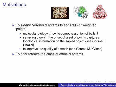
Motivations
I To extend Voronoi diagrams to spheres (or weightedpoints)
I molecular biology : how to compute a union of balls ?I sampling theory : the offset of a set of points captures
topological information on the sapled object (see Course F.Chazal)
I to improve the quality of a mesh (see Course M. Yvinec)I To characterize the class of affine diagrams
Winter School on Algorithmic Geometry Convex Hulls, Voronoi Diagrams and Delaunay Triangulations
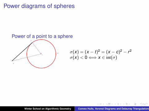
Power diagrams of spheres
Power of a point to a sphere
x
c
t
σ σ(x) = (x − t)2 = (x − c)2 − r2
σ(x) < 0⇐⇒ x ∈ int(σ)
Winter School on Algorithmic Geometry Convex Hulls, Voronoi Diagrams and Delaunay Triangulations
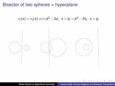
Bisector of two spheres = hyperplane
σi(x) = σj(x)⇐⇒6 x2 − 2ci · x + si =6 x2 − 2cj · x + sj
Winter School on Algorithmic Geometry Convex Hulls, Voronoi Diagrams and Delaunay Triangulations
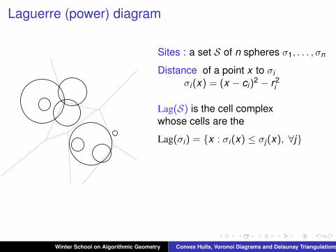
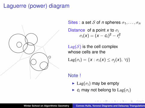
Laguerre (power) diagram
Sites : a set S of n spheres σ1, . . . , σn
Distance of a point x to σiσi(x) = (x − ci)
2 − r2i
Lag(S) is the cell complexwhose cells are the
Lag(σi) = {x : σi(x) ≤ σj(x), ∀j}
Note !I Lag(σi) may be emptyI ci may not belong to Lag(σi)
Winter School on Algorithmic Geometry Convex Hulls, Voronoi Diagrams and Delaunay Triangulations
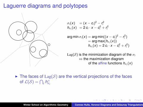
Laguerre diagrams and polytopes
σi(x) = (x − ci)2 − r 2
i
hσi (x) = 2 ci · x − c2i + r 2
i
arg minσi(x) = arg min((x − ci)2 − r 2
i )= arg max(hσi (x))hσi (x) = 2 ci · x − c2
i + r 2i )
Lag(S) is the minimization diagram of the σi
⇔ the maximization diagramof the affine functions hσi (x)
I The faces of Lag(S) are the vertical projections of the facesof L(S) =
⋂i h+σi
Winter School on Algorithmic Geometry Convex Hulls, Voronoi Diagrams and Delaunay Triangulations
Space of spheres
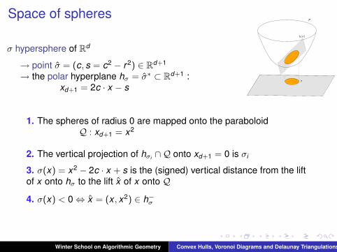
σ hypersphere of Rd
→ point σ = (c, s = c2 − r2) ∈ Rd+1
→ the polar hyperplane hσ = σ∗ ⊂ Rd+1 :xd+1 = 2c · x − s
σ
h(σ)
P
1. The spheres of radius 0 are mapped onto the paraboloidQ : xd+1 = x2
2. The vertical projection of hσi ∩Q onto xd+1 = 0 is σi
3. σ(x) = x2 − 2c · x + s is the (signed) vertical distance from the liftof x onto hσ to the lift x of x onto Q4. σ(x) < 0⇔ x = (x , x2) ∈ h−σ
Winter School on Algorithmic Geometry Convex Hulls, Voronoi Diagrams and Delaunay Triangulations
Orthogonality between spheres
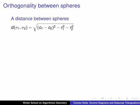
A distance between spheres
d(σ1, σ2) =√
(c1 − c2)2 − r21 − r2
2
Orthogonality
d(σ1, σ2) = 0⇔ (c1 − c2)2 = r21 + r2
2⇔ σ1 ⊥ σ2 (Pythagore)
In the space of spheres
d(σ1, σ2) = 0 ⇔ s2 = 2 c1 · c2 − c21 ⇔ σ2 ∈ hσ1 (si = c2
i − r2i )
< < h−σ1
σ
h(σ)
P
Winter School on Algorithmic Geometry Convex Hulls, Voronoi Diagrams and Delaunay Triangulations
Orthogonality between spheres
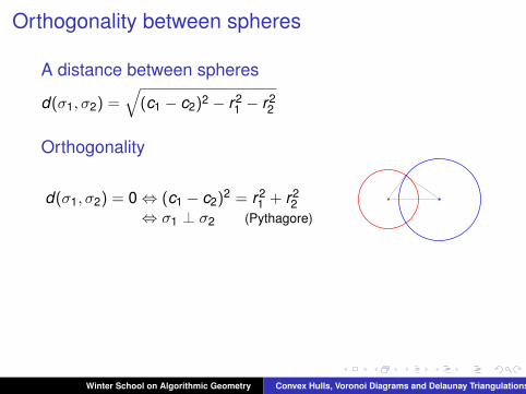
A distance between spheres
d(σ1, σ2) =√
(c1 − c2)2 − r21 − r2
2
Orthogonality
d(σ1, σ2) = 0⇔ (c1 − c2)2 = r21 + r2
2⇔ σ1 ⊥ σ2 (Pythagore)
In the space of spheres
d(σ1, σ2) = 0 ⇔ s2 = 2 c1 · c2 − c21 ⇔ σ2 ∈ hσ1 (si = c2
i − r2i )
< < h−σ1
σ
h(σ)
P
Winter School on Algorithmic Geometry Convex Hulls, Voronoi Diagrams and Delaunay Triangulations
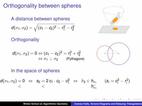
Orthogonality between spheres
A distance between spheres
d(σ1, σ2) =√
(c1 − c2)2 − r21 − r2
2
Orthogonality
d(σ1, σ2) = 0⇔ (c1 − c2)2 = r21 + r2
2⇔ σ1 ⊥ σ2 (Pythagore)
In the space of spheres
d(σ1, σ2) = 0 ⇔ s2 = 2 c1 · c2 − c21 ⇔ σ2 ∈ hσ1 (si = c2
i − r2i )
< < h−σ1
σ
h(σ)
P
Winter School on Algorithmic Geometry Convex Hulls, Voronoi Diagrams and Delaunay Triangulations
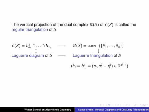
The vertical projection of the dual complex R(S) of L(S) is called theregular triangulation of S
L(S) = h+σ1∩ . . . ∩ h+
σn←→ R(S) = conv−({σ1, . . . , σn})
l lLaguerre diagram of S ←→ Laguerre triangulation of S
(σi = h∗σi= (ci , c2
i − r2i ) ∈ Rd+1)
Winter School on Algorithmic Geometry Convex Hulls, Voronoi Diagrams and Delaunay Triangulations
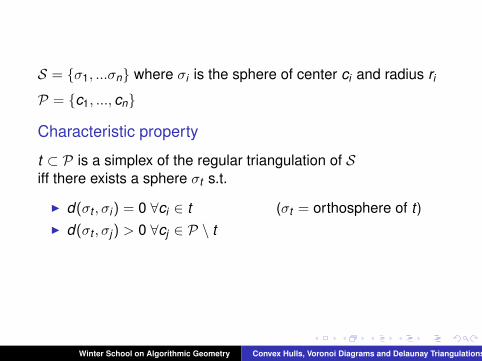
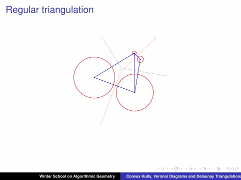
S = {σ1, ...σn} where σi is the sphere of center ci and radius ri
P = {c1, ..., cn}
Characteristic property
t ⊂ P is a simplex of the regular triangulation of Siff there exists a sphere σt s.t.
I d(σt , σi) = 0 ∀ci ∈ t (σt = orthosphere of t)I d(σt , σj) > 0 ∀cj ∈ P \ t
Winter School on Algorithmic Geometry Convex Hulls, Voronoi Diagrams and Delaunay Triangulations
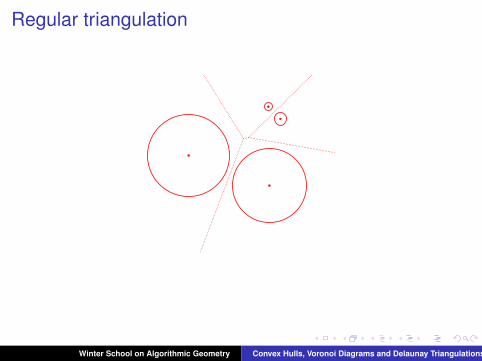
Regular triangulation
Winter School on Algorithmic Geometry Convex Hulls, Voronoi Diagrams and Delaunay Triangulations
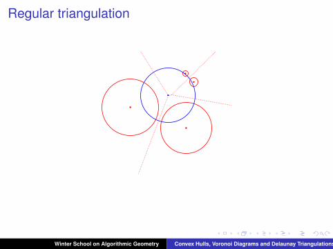
Regular triangulation
Winter School on Algorithmic Geometry Convex Hulls, Voronoi Diagrams and Delaunay Triangulations
Regular triangulation
Winter School on Algorithmic Geometry Convex Hulls, Voronoi Diagrams and Delaunay Triangulations
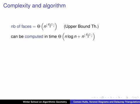
Complexity and algorithm
nb of faces = Θ(
nbd+1
2 c)
(Upper Bound Th.)
can be computed in time Θ(
n log n + nbd+1
2 c)
Main predicate
power test(σ0, . . . , σd+1) = sign
∣∣∣∣∣∣1 . . . 1c0 . . . cd+1
c20 − r2
0 . . . c2d+1 − r2
d+1
∣∣∣∣∣∣
Winter School on Algorithmic Geometry Convex Hulls, Voronoi Diagrams and Delaunay Triangulations
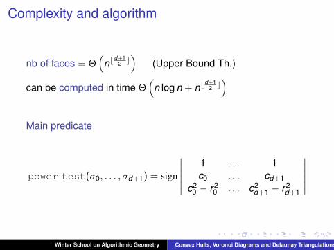
Complexity and algorithm
nb of faces = Θ(
nbd+1
2 c)
(Upper Bound Th.)
can be computed in time Θ(
n log n + nbd+1
2 c)
Main predicate
power test(σ0, . . . , σd+1) = sign
∣∣∣∣∣∣1 . . . 1c0 . . . cd+1
c20 − r2
0 . . . c2d+1 − r2
d+1
∣∣∣∣∣∣
Winter School on Algorithmic Geometry Convex Hulls, Voronoi Diagrams and Delaunay Triangulations
Affine diagrams and regular subdivisions
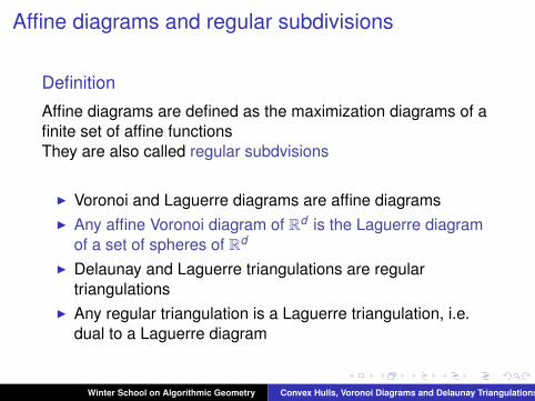
Definition
Affine diagrams are defined as the maximization diagrams of afinite set of affine functionsThey are also called regular subdvisions
I Voronoi and Laguerre diagrams are affine diagramsI Any affine Voronoi diagram of Rd is the Laguerre diagram
of a set of spheres of Rd
I Delaunay and Laguerre triangulations are regulartriangulations
I Any regular triangulation is a Laguerre triangulation, i.e.dual to a Laguerre diagram
Winter School on Algorithmic Geometry Convex Hulls, Voronoi Diagrams and Delaunay Triangulations
Affine diagrams and regular subdivisions
Definition
Affine diagrams are defined as the maximization diagrams of afinite set of affine functionsThey are also called regular subdvisions
I Voronoi and Laguerre diagrams are affine diagramsI Any affine Voronoi diagram of Rd is the Laguerre diagram
of a set of spheres of Rd
I Delaunay and Laguerre triangulations are regulartriangulations
I Any regular triangulation is a Laguerre triangulation, i.e.dual to a Laguerre diagram
Winter School on Algorithmic Geometry Convex Hulls, Voronoi Diagrams and Delaunay Triangulations
Examples of affine diagrams
1. The intersection of a power diagram with an affinesubspace
2. A Voronoi diagram with the following quadratic distancefunction
‖x − a‖Q = (x − a)tQ(x − a) Q = Qt
3. k -th order Voronoi diagrams
Winter School on Algorithmic Geometry Convex Hulls, Voronoi Diagrams and Delaunay Triangulations
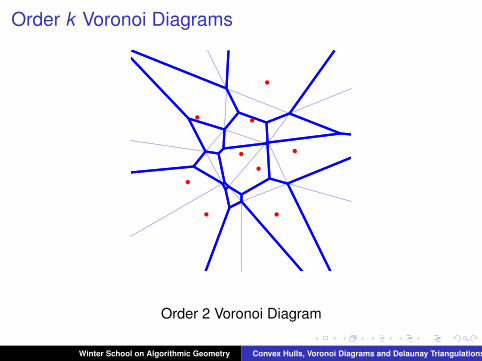
Order k Voronoi Diagrams
Order 2 Voronoi Diagram
Winter School on Algorithmic Geometry Convex Hulls, Voronoi Diagrams and Delaunay Triangulations
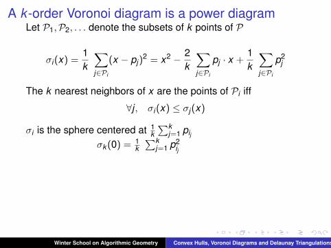
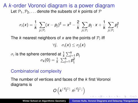
A k -order Voronoi diagram is a power diagramLet P1,P2, . . . denote the subsets of k points of P
σi(x) =1k
∑j∈Pi
(x − pj)2 = x2 − 2
k
∑j∈Pi
pj · x +1k
∑j∈Pi
p2j
The k nearest neighbors of x are the points of Pi iff
∀j , σi(x) ≤ σj(x)
σi is the sphere centered at 1k∑k
j=1 pijσk (0) = 1
k∑k
j=1 p2ij
Combinatorial complexity
The number of vertices and faces of the k first Voronoidiagrams is
O(
kdd+1
2 e nbd+1
2 c)
Winter School on Algorithmic Geometry Convex Hulls, Voronoi Diagrams and Delaunay Triangulations
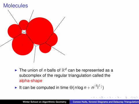
Molecules
I The union of n balls of Rd can be represented as asubcomplex of the regular triangulation called thealpha-shape
I It can be computed in time Θ(n log n + nbd+1
2 c)
Winter School on Algorithmic Geometry Convex Hulls, Voronoi Diagrams and Delaunay Triangulations
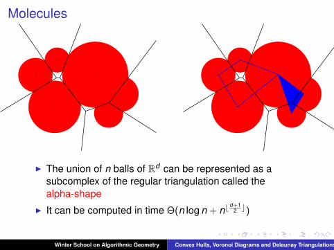
Molecules
I The union of n balls of Rd can be represented as asubcomplex of the regular triangulation called thealpha-shape
I It can be computed in time Θ(n log n + nbd+1
2 c)
Winter School on Algorithmic Geometry Convex Hulls, Voronoi Diagrams and Delaunay Triangulations
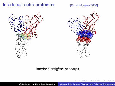
Interfaces entre proteines [Cazals & Janin 2006]
Interface antigene-anticorps
Winter School on Algorithmic Geometry Convex Hulls, Voronoi Diagrams and Delaunay Triangulations
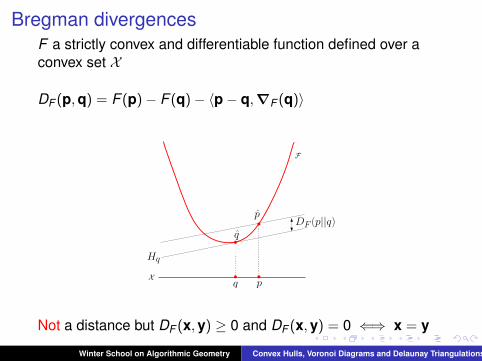
Bregman divergencesF a strictly convex and differentiable function defined over aconvex set X
DF (p,q) = F (p)− F (q)− 〈p− q,∇F (q)〉
F
Xpq
p
q
Hq
DF (p||q)
Not a distance but DF (x,y) ≥ 0 and DF (x,y) = 0 ⇐⇒ x = y
Winter School on Algorithmic Geometry Convex Hulls, Voronoi Diagrams and Delaunay Triangulations
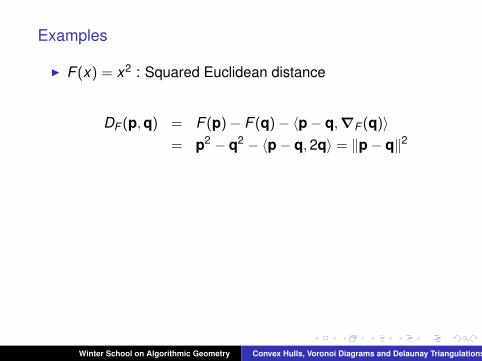
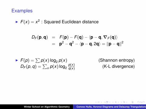
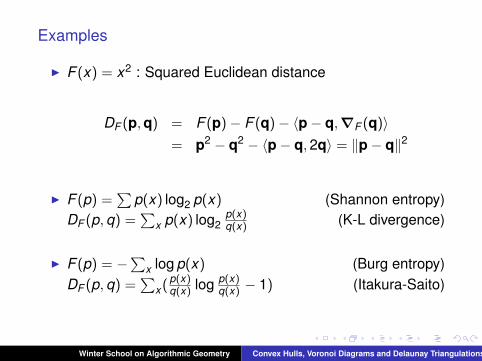
Examples
I F (x) = x2 : Squared Euclidean distance
DF (p,q) = F (p)− F (q)− 〈p− q,∇F (q)〉= p2 − q2 − 〈p− q,2q〉 = ‖p− q‖2
I F (p) =∑
p(x) log2 p(x) (Shannon entropy)DF (p,q) =
∑x p(x) log2
p(x)q(x) (K-L divergence)
I F (p) = −∑x log p(x) (Burg entropy)DF (p,q) =
∑x ( p(x)
q(x) log p(x)q(x) − 1) (Itakura-Saito)
Winter School on Algorithmic Geometry Convex Hulls, Voronoi Diagrams and Delaunay Triangulations
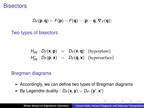
Bisectors
DF (p,q) = F (p)− F (q)− 〈p− q,∇F (q)〉
Two types of bisectors
Hpq : DF (x,p) = DF (x,q) (hyperplane)
H∗pq : DF (p,x) = DF (q,x) (hypersurface)
Bregman diagrams
I Accordingly, we can define two types of Bregman diagramsI By Legendre duality : DF (x,y) = DF∗(y′,x′)
Winter School on Algorithmic Geometry Convex Hulls, Voronoi Diagrams and Delaunay Triangulations
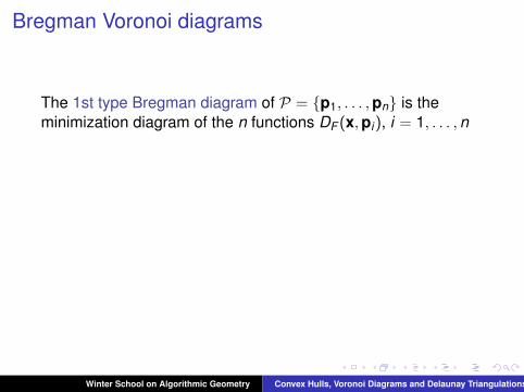
Bregman Voronoi diagrams
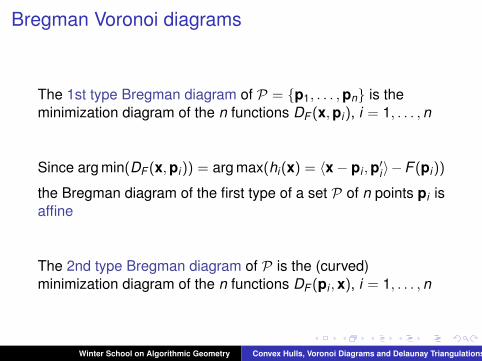
The 1st type Bregman diagram of P = {p1, . . . ,pn} is theminimization diagram of the n functions DF (x,pi), i = 1, . . . ,n
Since arg min(DF (x,pi)) = arg max(hi(x) = 〈x− pi ,p′i〉−F (pi))
the Bregman diagram of the first type of a set P of n points pi isaffine
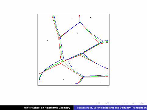
The 2nd type Bregman diagram of P is the (curved)minimization diagram of the n functions DF (pi ,x), i = 1, . . . ,n
Winter School on Algorithmic Geometry Convex Hulls, Voronoi Diagrams and Delaunay Triangulations
Bregman Voronoi diagrams
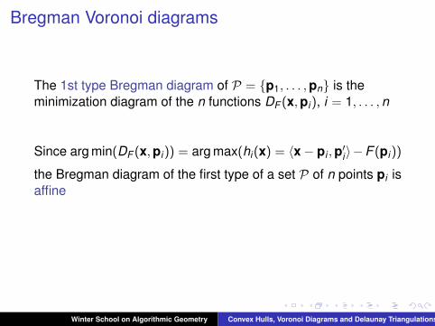
The 1st type Bregman diagram of P = {p1, . . . ,pn} is theminimization diagram of the n functions DF (x,pi), i = 1, . . . ,n
Since arg min(DF (x,pi)) = arg max(hi(x) = 〈x− pi ,p′i〉−F (pi))
the Bregman diagram of the first type of a set P of n points pi isaffine
The 2nd type Bregman diagram of P is the (curved)minimization diagram of the n functions DF (pi ,x), i = 1, . . . ,n
Winter School on Algorithmic Geometry Convex Hulls, Voronoi Diagrams and Delaunay Triangulations
Bregman Voronoi diagrams
The 1st type Bregman diagram of P = {p1, . . . ,pn} is theminimization diagram of the n functions DF (x,pi), i = 1, . . . ,n
Since arg min(DF (x,pi)) = arg max(hi(x) = 〈x− pi ,p′i〉−F (pi))
the Bregman diagram of the first type of a set P of n points pi isaffine
The 2nd type Bregman diagram of P is the (curved)minimization diagram of the n functions DF (pi ,x), i = 1, . . . ,n
Winter School on Algorithmic Geometry Convex Hulls, Voronoi Diagrams and Delaunay Triangulations
Winter School on Algorithmic Geometry Convex Hulls, Voronoi Diagrams and Delaunay Triangulations
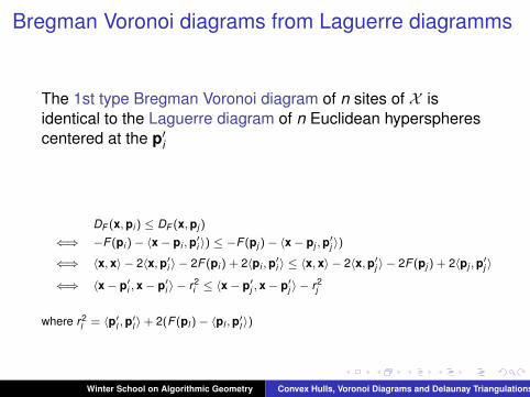
Bregman Voronoi diagrams from Laguerre diagramms
The 1st type Bregman Voronoi diagram of n sites of X isidentical to the Laguerre diagram of n Euclidean hyperspherescentered at the p′i
DF (x,pi ) ≤ DF (x,pj )
⇐⇒ −F (pi )− 〈x− pi ,p′i 〉) ≤ −F (pj )− 〈x− pj ,p′j 〉)
⇐⇒ 〈x, x〉 − 2〈x,p′i 〉 − 2F (pi ) + 2〈pi ,p′i 〉 ≤ 〈x, x〉 − 2〈x,p′j 〉 − 2F (pj ) + 2〈pj ,p′j 〉
⇐⇒ 〈x− p′i , x− p′i 〉 − r2i ≤ 〈x− p′j , x− p′j 〉 − r2
j
where r2l = 〈p′l ,p
′l 〉+ 2(F (pl )− 〈pl ,p′l 〉)
Winter School on Algorithmic Geometry Convex Hulls, Voronoi Diagrams and Delaunay Triangulations
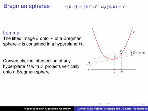
Bregman spheres σ(c, r) = {x ∈ X | DF (x,c) = r}
LemmaThe lifted image σ onto F of a Bregmansphere σ is contained in a hyperplane Hσ
Conversely, the intersection of anyhyperplane H with F projects verticallyonto a Bregman sphere
F
Xpq
p
q
Hq
DF (p||q)
Winter School on Algorithmic Geometry Convex Hulls, Voronoi Diagrams and Delaunay Triangulations
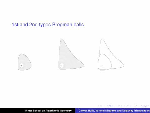
1st and 2nd types Bregman balls
Winter School on Algorithmic Geometry Convex Hulls, Voronoi Diagrams and Delaunay Triangulations
Bregman triangulations
P : the lifted image of P onto the graph F of F
T the lower convex hull of P
The vertical projection of T is called the Bregman triangulationBTF (P) of P
Characteristic property
The Bregman sphere circumscribing any simplex of BTF (P)does not enclose any point of P
Winter School on Algorithmic Geometry Convex Hulls, Voronoi Diagrams and Delaunay Triangulations
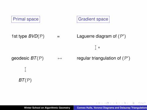
Primal space Gradient space
1st type BVD(P) = Laguerre diagram of (P ′)
l ∗
geodesic BT (P) ↔ regular triangulation of (P ′)
l
BT (P)
Winter School on Algorithmic Geometry Convex Hulls, Voronoi Diagrams and Delaunay Triangulations
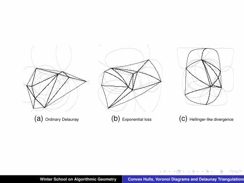
(a) Ordinary Delaunay (b) Exponential loss (c) Hellinger-like divergence
Winter School on Algorithmic Geometry Convex Hulls, Voronoi Diagrams and Delaunay Triangulations
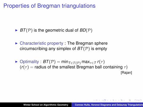
Properties of Bregman triangulations
I BT (P) is the geometric dual of BD(P)
I Characteristic property : The Bregman spherecircumscribing any simplex of BT (P) is empty
I Optimality : BT (P) = minT∈T (P) maxτ∈T r(τ)(r(τ) = radius of the smallest Bregman ball containing τ )
[Rajan]
Winter School on Algorithmic Geometry Convex Hulls, Voronoi Diagrams and Delaunay Triangulations


![Domain Specific Languages [0.5ex] for Convex Optimization](https://static.fdocument.org/doc/165x107/61fb7d612e268c58cd5ec7a1/domain-specific-languages-05ex-for-convex-optimization.jpg)
![Lecture 6 - Convex Sets - Drexel Universitytyu/Math690Optimization/lec... · 2020. 4. 28. · Lecture 6 - Convex Sets De nitionA set C Rn is calledconvexif for any x;y 2C and 2[0;1],](https://static.fdocument.org/doc/165x107/5fd34e0aa8df85529a7479e7/lecture-6-convex-sets-drexel-university-tyumath690optimizationlec-2020.jpg)