Primal-Dual Interior-Point Methods

Ryan TibshiraniConvex Optimization 10-725

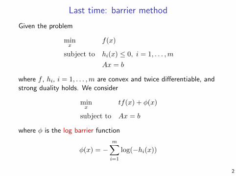
Last time: barrier method

Given the problem

minx

f(x)

subject to hi(x) ≤ 0, i = 1, . . . ,m

Ax = b

where f , hi, i = 1, . . . ,m are convex and twice differentiable, andstrong duality holds. We consider

minx

tf(x) + φ(x)

subject to Ax = b

where φ is the log barrier function

φ(x) = −m∑

i=1

log(−hi(x))

2

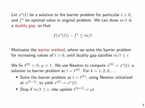
Let x?(t) be a solution to the barrier problem for particular t > 0,and f? be optimal value in original problem. We can show m/t isa duality gap, so that

f(x?(t))− f? ≤ m/t

Motivates the barrier method, where we solve the barrier problemfor increasing values of t > 0, until duality gap satisfies m/t ≤ ε

We fix t(0) > 0, µ > 1. We use Newton to compute x(0) = x?(t), asolution to barrier problem at t = t(0). For k = 1, 2, 3, . . .

• Solve the barrier problem at t = t(k), using Newton initializedat x(k−1), to yield x(k) = x?(t)

• Stop if m/t ≤ ε, else update t(k+1) = µt

3

Outline

Today:

• Perturbed KKT conditions, revisited

• Primal-dual interior-point method

• Backtracking line search

• Highlight on standard form LPs

4

Barrier versus primal-dual method

Today we will discuss the primal-dual interior-point method, whichsolves basically the same problems as the barrier method. What’sthe difference between these two?

Overview:

• Both can be motivated in terms of perturbed KKT conditions

• Primal-dual interior-point methods take one Newton step, andmove on (no separate inner and outer loops)

• Primal-dual interior-point iterates are not necessarily feasible

• Primal-dual interior-point methods are often more efficient, asthey can exhibit better than linear convergence

• Primal-dual interior-point methods are less intuitive ...

5

Perturbed KKT conditions

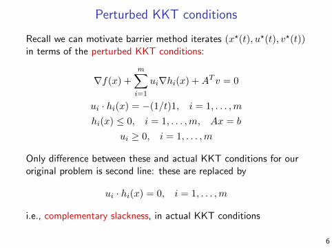
Recall we can motivate barrier method iterates (x?(t), u?(t), v?(t))in terms of the perturbed KKT conditions:

∇f(x) +

m∑

i=1

ui∇hi(x) +AT v = 0

ui · hi(x) = −(1/t)1, i = 1, . . . ,m

hi(x) ≤ 0, i = 1, . . . ,m, Ax = b

ui ≥ 0, i = 1, . . . ,m

Only difference between these and actual KKT conditions for ouroriginal problem is second line: these are replaced by

ui · hi(x) = 0, i = 1, . . . ,m

i.e., complementary slackness, in actual KKT conditions

6

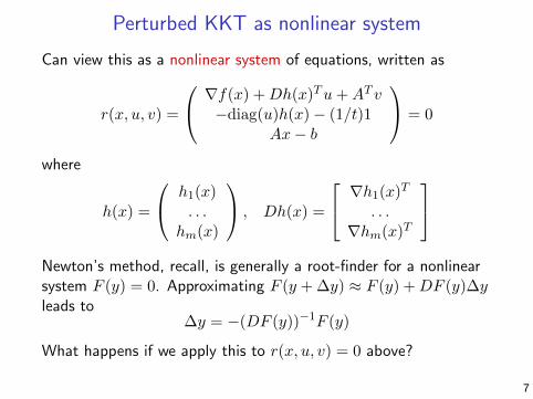
Perturbed KKT as nonlinear system

Can view this as a nonlinear system of equations, written as

r(x, u, v) =

∇f(x) +Dh(x)Tu+AT v−diag(u)h(x)− (1/t)1

Ax− b

= 0

where

h(x) =

h1(x). . .

hm(x)

, Dh(x) =

∇h1(x)T

. . .∇hm(x)T

Newton’s method, recall, is generally a root-finder for a nonlinearsystem F (y) = 0. Approximating F (y + ∆y) ≈ F (y) +DF (y)∆yleads to

∆y = −(DF (y))−1F (y)

What happens if we apply this to r(x, u, v) = 0 above?

7

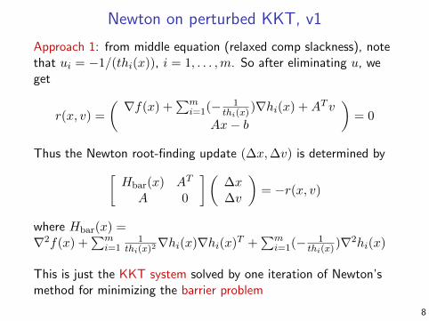
Newton on perturbed KKT, v1

Approach 1: from middle equation (relaxed comp slackness), notethat ui = −1/(thi(x)), i = 1, . . . ,m. So after eliminating u, weget

r(x, v) =

( ∇f(x) +∑m

i=1(− 1thi(x)

)∇hi(x) +AT v

Ax− b

)= 0

Thus the Newton root-finding update (∆x,∆v) is determined by

[Hbar(x) AT

A 0

](∆x∆v

)= −r(x, v)

where Hbar(x) =∇2f(x) +

∑mi=1

1thi(x)2

∇hi(x)∇hi(x)T +∑m

i=1(− 1thi(x)

)∇2hi(x)

This is just the KKT system solved by one iteration of Newton’smethod for minimizing the barrier problem

8

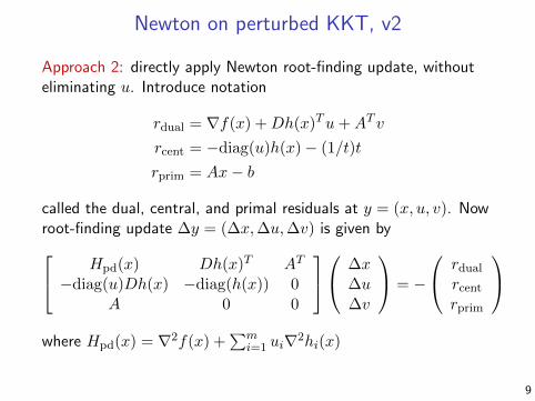
Newton on perturbed KKT, v2

Approach 2: directly apply Newton root-finding update, withouteliminating u. Introduce notation

rdual = ∇f(x) +Dh(x)Tu+AT v

rcent = −diag(u)h(x)− (1/t)t

rprim = Ax− b

called the dual, central, and primal residuals at y = (x, u, v). Nowroot-finding update ∆y = (∆x,∆u,∆v) is given by

Hpd(x) Dh(x)T AT

−diag(u)Dh(x) −diag(h(x)) 0A 0 0

∆x∆u∆v

= −

rdualrcentrprim

where Hpd(x) = ∇2f(x) +∑m

i=1 ui∇2hi(x)

9

Some notes:

• In v2, update directions for the primal and dual variables areinexorably linked together

• Also, v2 and v1 leads to different (nonequivalent) updates

• As we saw, one iteration of v1 is equivalent to inner iterationin the barrier method

• And v2 defines a new method called primal-dual interior-pointmethod, that we will flesh out shortly

• One complication: in v2, the dual iterates are not necessarilyfeasible for the original dual problem ...

10

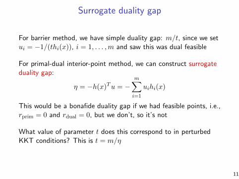
Surrogate duality gap

For barrier method, we have simple duality gap: m/t, since we setui = −1/(thi(x)), i = 1, . . . ,m and saw this was dual feasible

For primal-dual interior-point method, we can construct surrogateduality gap:

η = −h(x)Tu = −m∑

i=1

uihi(x)

This would be a bonafide duality gap if we had feasible points, i.e.,rprim = 0 and rdual = 0, but we don’t, so it’s not

What value of parameter t does this correspond to in perturbedKKT conditions? This is t = m/η

11

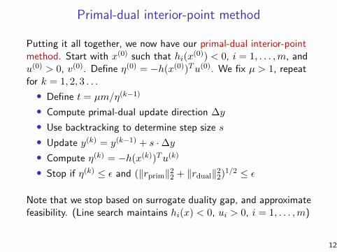
Primal-dual interior-point method

Putting it all together, we now have our primal-dual interior-pointmethod. Start with x(0) such that hi(x

(0)) < 0, i = 1, . . . ,m, andu(0) > 0, v(0). Define η(0) = −h(x(0))Tu(0). We fix µ > 1, repeatfor k = 1, 2, 3 . . .

• Define t = µm/η(k−1)

• Compute primal-dual update direction ∆y

• Use backtracking to determine step size s

• Update y(k) = y(k−1) + s ·∆y• Compute η(k) = −h(x(k))Tu(k)

• Stop if η(k) ≤ ε and (‖rprim‖22 + ‖rdual‖22)1/2 ≤ ε

Note that we stop based on surrogate duality gap, and approximatefeasibility. (Line search maintains hi(x) < 0, ui > 0, i = 1, . . . ,m)

12

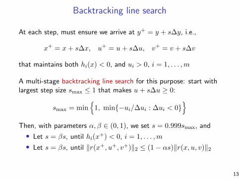
Backtracking line search

At each step, must ensure we arrive at y+ = y + s∆y, i.e.,

x+ = x+ s∆x, u+ = u+ s∆u, v+ = v + s∆v

that maintains both hi(x) < 0, and ui > 0, i = 1, . . . ,m

A multi-stage backtracking line search for this purpose: start withlargest step size smax ≤ 1 that makes u+ s∆u ≥ 0:

smax = min{

1, min{−ui/∆ui : ∆ui < 0}}

Then, with parameters α, β ∈ (0, 1), we set s = 0.999smax, and

• Let s = βs, until hi(x+) < 0, i = 1, . . . ,m

• Let s = βs, until ‖r(x+, u+, v+)‖2 ≤ (1− αs)‖r(x, u, v)‖2

13

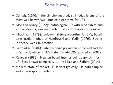
Some history

• Dantzig (1940s): the simplex method, still today is one of themost well-known/well-studied algorithms for LPs

• Klee and Minty (1972): pathological LP with n variables and2n constraints, simplex method takes 2n iterations to solve

• Khachiyan (1979): polynomial-time algorithm for LPs, basedon ellipsoid method of Nemirovski and Yudin (1976). Strongin theory, weak in practice

• Karmarkar (1984): interior-point polynomial-time method forLPs. Fairly efficient (US Patent 4,744,026, expired in 2006)

• Renegar (1988): Newton-based interior-point algorithm forLP. Best known complexity ... until Lee and Sidford (2014)

• Modern state-of-the-art LP solvers typically use both simplexand interior-point methods

14

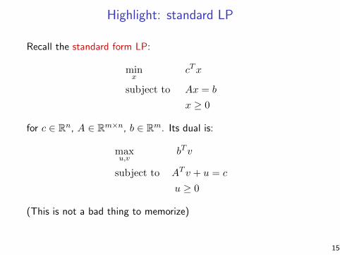
Highlight: standard LP

Recall the standard form LP:

minx

cTx

subject to Ax = b

x ≥ 0

for c ∈ Rn, A ∈ Rm×n, b ∈ Rm. Its dual is:

maxu,v

bT v

subject to AT v + u = c

u ≥ 0

(This is not a bad thing to memorize)

15

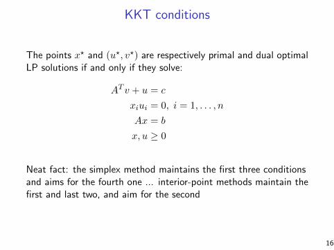
KKT conditions

The points x? and (u?, v?) are respectively primal and dual optimalLP solutions if and only if they solve:

AT v + u = c

xiui = 0, i = 1, . . . , n

Ax = b

x, u ≥ 0

Neat fact: the simplex method maintains the first three conditionsand aims for the fourth one ... interior-point methods maintain thefirst and last two, and aim for the second

16

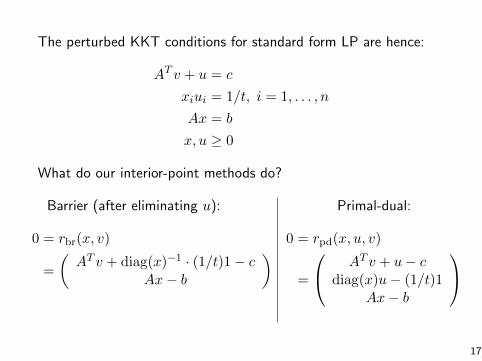
The perturbed KKT conditions for standard form LP are hence:

AT v + u = c

xiui = 1/t, i = 1, . . . , n

Ax = b

x, u ≥ 0

What do our interior-point methods do?

Barrier (after eliminating u):

0 = rbr(x, v)

=

(AT v + diag(x)−1 · (1/t)1− c

Ax− b

)

Primal-dual:

0 = rpd(x, u, v)

=

AT v + u− cdiag(x)u− (1/t)1

Ax− b

17

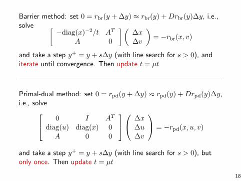
Barrier method: set 0 = rbr(y + ∆y) ≈ rbr(y) +Drbr(y)∆y, i.e.,solve [

−diag(x)−2/t AT

A 0

](∆x∆v

)= −rbr(x, v)

and take a step y+ = y + s∆y (with line search for s > 0), anditerate until convergence. Then update t = µt

Primal-dual method: set 0 = rpd(y + ∆y) ≈ rpd(y) +Drpd(y)∆y,i.e., solve

0 I AT

diag(u) diag(x) 0A 0 0

∆x∆u∆v

= −rpd(x, u, v)

and take a step y+ = y + s∆y (with line search for s > 0), butonly once. Then update t = µt

18

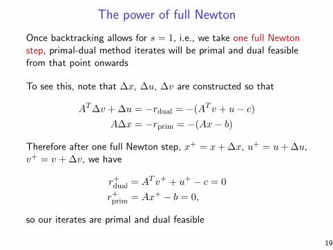
The power of full Newton

Once backtracking allows for s = 1, i.e., we take one full Newtonstep, primal-dual method iterates will be primal and dual feasiblefrom that point onwards

To see this, note that ∆x, ∆u, ∆v are constructed so that

AT∆v + ∆u = −rdual = −(AT v + u− c)A∆x = −rprim = −(Ax− b)

Therefore after one full Newton step, x+ = x+ ∆x, u+ = u+ ∆u,v+ = v + ∆v, we have

r+dual = AT v+ + u+ − c = 0

r+prim = Ax+ − b = 0,

so our iterates are primal and dual feasible

19

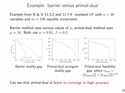
Example: barrier versus primal-dual

Example from B & V 11.3.2 and 11.7.4: standard LP with n = 50variables and m = 100 equality constraints

Barrier method uses various values of µ, primal-dual method usesµ = 10. Both use α = 0.01, β = 0.5

572 11 Interior-point methods

Newton iterations

dual

ity

gap

µ = 2µ = 50 µ = 150

0 20 40 60 80

10−6

10−4

10−2

100

102

Figure 11.4 Progress of barrier method for a small LP, showing dualitygap versus cumulative number of Newton steps. Three plots are shown,corresponding to three values of the parameter µ: 2, 50, and 150. In eachcase, we have approximately linear convergence of duality gap.

Newton’s method is λ(x)2/2 ≤ 10−5, where λ(x) is the Newton decrement of thefunction tcT x + φ(x).

The progress of the barrier method, for three values of the parameter µ, isshown in figure 11.4. The vertical axis shows the duality gap on a log scale. Thehorizontal axis shows the cumulative total number of inner iterations, i.e., Newtonsteps, which is the natural measure of computational effort. Each of the plots hasa staircase shape, with each stair associated with one outer iteration. The width ofeach stair tread (i.e., horizontal portion) is the number of Newton steps requiredfor that outer iteration. The height of each stair riser (i.e., the vertical portion) isexactly equal to (a factor of) µ, since the duality gap is reduced by the factor µ atthe end of each outer iteration.

The plots illustrate several typical features of the barrier method. First of all,the method works very well, with approximately linear convergence of the dualitygap. This is a consequence of the approximately constant number of Newton stepsrequired to re-center, for each value of µ. For µ = 50 and µ = 150, the barriermethod solves the problem with a total number of Newton steps between 35 and 40.

The plots in figure 11.4 clearly show the trade-off in the choice of µ. For µ = 2,the treads are short; the number of Newton steps required to re-center is around 2or 3. But the risers are also short, since the duality gap reduction per outer iterationis only a factor of 2. At the other extreme, when µ = 150, the treads are longer,typically around 7 Newton steps, but the risers are also much larger, since theduality gap is reduced by the factor 150 in each outer iteration.

The trade-off in choice of µ is further examined in figure 11.5. We use thebarrier method to solve the LP, terminating when the duality gap is smaller than10−3, for 25 values of µ between 1.2 and 200. The plot shows the total numberof Newton steps required to solve the problem, as a function of the parameter µ.

614 11 Interior-point methods

iteration number

η̂

0 5 10 15 20 25 3010−10

10−8

10−6

10−4

10−2

100

102

iteration number

r feas

0 5 10 15 20 25 30

10−15

10−10

10−5

100

105

Figure 11.21 Progress of the primal-dual interior-point method for an LP,showing surrogate duality gap η̂ and the norm of the primal and dual resid-uals, versus iteration number. The residual converges rapidly to zero within24 iterations; the surrogate gap also converges to a very small number inabout 28 iterations. The primal-dual interior-point method converges fasterthan the barrier method, especially if high accuracy is required.

iteration number

η̂

0 5 10 15 20 2510−10

10−8

10−6

10−4

10−2

100

102

iteration number

r feas

0 5 10 15 20 2510−15

10−10

10−5

100

105

Figure 11.22 Progress of primal-dual interior-point method for a GP, show-ing surrogate duality gap η̂ and the norm of the primal and dual residualsversus iteration number.

614 11 Interior-point methods

iteration number

η̂

0 5 10 15 20 25 3010−10

10−8

10−6

10−4

10−2

100

102

iteration number

r feas

0 5 10 15 20 25 30

10−15

10−10

10−5

100

105

Figure 11.21 Progress of the primal-dual interior-point method for an LP,showing surrogate duality gap η̂ and the norm of the primal and dual resid-uals, versus iteration number. The residual converges rapidly to zero within24 iterations; the surrogate gap also converges to a very small number inabout 28 iterations. The primal-dual interior-point method converges fasterthan the barrier method, especially if high accuracy is required.

iteration number

η̂

0 5 10 15 20 2510−10

10−8

10−6

10−4

10−2

100

102

iteration number

r feas

0 5 10 15 20 2510−15

10−10

10−5

100

105

Figure 11.22 Progress of primal-dual interior-point method for a GP, show-ing surrogate duality gap η̂ and the norm of the primal and dual residualsversus iteration number.

Barrier duality gap Primal-dual surrogateduality gap

Primal-dual feasibilitygap, where rfeas =

(‖rprim‖22 + ‖rdual‖22)1/2

Can see that primal-dual is faster to converge to high accuracy

20

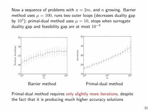
Now a sequence of problems with n = 2m, and n growing. Barriermethod uses µ = 100, runs two outer loops (decreases duality gapby 104); primal-dual method uses µ = 10, stops when surrogateduality gap and feasibility gap are at most 10−8

576 11 Interior-point methods

Newton iterations

dual

ity

gap

m = 50 m = 500m = 1000

0 10 20 30 40 5010−4

10−2

100

102

104

Figure 11.7 Progress of barrier method for three randomly generated stan-dard form LPs of different dimensions, showing duality gap versus cumula-tive number of Newton steps. The number of variables in each problem isn = 2m. Here too we see approximately linear convergence of the dualitygap, with a slight increase in the number of Newton steps required for thelarger problems.

m

New

ton

iter

atio

ns

101 102 10315

20

25

30

35

Figure 11.8 Average number of Newton steps required to solve 100 randomlygenerated LPs of different dimensions, with n = 2m. Error bars show stan-dard deviation, around the average value, for each value of m. The growthin the number of Newton steps required, as the problem dimensions rangeover a 100:1 ratio, is very small.

11.8 Implementation 615

miter

atio

ns

101 102 10310

20

30

40

50

Figure 11.23 Number of iterations required to solve randomly generatedstandard LPs of different dimensions, with n = 2m. Error bars show stan-dard deviation, around the average value, for 100 instances of each dimen-sion. The growth in the number of iterations required, as the problem di-mensions range over a 100:1 ratio, is approximately logarithmic.

A family of LPs

Here we examine the performance of the primal-dual method as a function ofthe problem dimensions, for the same family of standard form LPs consideredin §11.3.2. We use the primal-dual interior-point method to solve the same 2000instances, which consist of 100 instances for each value of m. The primal-dualalgorithm is started at x(0) = 1, λ(0) = 1, ν(0) = 0, and terminated using toleranceϵ = 10−8. Figure 11.23 shows the average, and standard deviation, of the numberof iterations required versus m. The number of iterations ranges from 15 to 35,and grows approximately as the logarithm of m. Comparing with the results forthe barrier method shown in figure 11.8, we see that the number of iterations inthe primal-dual method is only slightly higher, despite the fact that we start atinfeasible starting points, and solve the problem to a much higher accuracy.

11.8 Implementation

The main effort in the barrier method is computing the Newton step for the cen-tering problem, which consists of solving sets of linear equations of the form

!H AT

A 0

" !∆xnt

νnt

"= −

!g0

", (11.60)

where

H = t∇2f0(x) +

m#

i=1

1

fi(x)2∇fi(x)∇fi(x)T +

m#

i=1

1

−fi(x)∇2fi(x)

Barrier method Primal-dual method

Primal-dual method requires only slightly more iterations, despitethe fact that it is producing much higher accuracy solutions

21

References and further reading

• S. Boyd and L. Vandenberghe (2004), “Convex optimization,”Chapter 11

• J. Nocedal and S. Wright (2006), “Numerical optimization”,Chapters 14 and 19

• J. Renegar (2001), “A mathematical view of interior-pointmethods”

• S. Wright (1997), “Primal-dual interior-point methods,”Chapters 5 and 6

22