PPNS.1 Pressure Projection Algorithms for...

PPNS.1 Pressure Projection Algorithms for INS

Pressure projection: INS methods enforcing only DMh

DMh: yiterativel0ε0 >≤⋅∇⇒=⋅∇ hh uu

“famous” named algorithms in the class include

MAC, SMAC – Los Alamos Nat. LabSIMPLE,- ER, -EC, -EST – Imperial College, UKPISO – Imperial College, UK Operator splitting – Univ. Houston Continuity constraint – Univ. Tennessee

fundamental PPNS theory ingredients

1. measure error in ∇h⋅uh via a potential function φh

2. employ φh to moderate DMh and/or DPh error via ⋅ velocity correction ⋅ pressure correction

3. iterate DPh + DMh until ε≤⋅∇ hh u 4. determine genuine pressure field

S e e k a s t r a t e g y t o i t e r a t e D M h + D P h f o r q = { u , p }

0Pe)(:D

0gReGrReδρ)(:D

0)(:D

1

110

0

=−⎟⎟⎠

⎞⎜⎜⎝

⎛

∂Θ∂

−Θ∂∂

+∂Θ∂

=Θ

=Θ+⎟⎟⎠

⎞⎜⎜⎝

⎛

∂∂

−+∂∂

+∂∂

=

=⋅∇=

−

−−

sx

uxt

E

xupuu

xtuu

M

jj

j

ij

iijij

j

ii

L

L

L

P

uρ

M arch DP h forward in tim e

definitionby0and

)(Re:TS

Denforcecantocorrectionaassumelikelyhoodallin0~:D

)(Reδρ

)(21~:TS

1

2*

11

*

1

2110

32

221

=⋅∇

Δ+∂∂

+⎥⎥⎦

⎤

⎢⎢⎣

⎡

∂∂

−∂∂

Δ−=

⇒⇒

≠⋅∇

Δ+⎥⎥⎦

⎤

⎢⎢⎣

⎡

∂∂

−+∂∂

Δ−=

Δ+∂∂

Δ+∂∂

Δ+=

+

−+

+

−−

+

ni

ij

nin

inj

j

ni

ni

n

n

j

ni

ijnn

inj

j

ni

n

i

n

ini

ni

u

tOxP

xuuu

xtuu

MPpM

tOxupuu

xtu

tOtut

tutuu

u

PPNS.2 Pressure Projection Foundation for INS

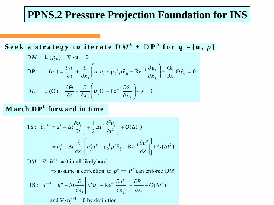
Subtracting the two TSs, one obtains

This explicit TS basis is theoretically inappropriate

( )

potentialMany

tO

tOPpx

tuu

h

nnn

nn

n

i

ni

ni

velocityaallymathematic isDinerrortheand

~!for~henceal,irrotationiscurlvanishingwithfieldvelocity

0)~()(toyieldssidesbothofcurlthetaking

)(ρ~

111

11

2

2*10

11

+++

++

−++

φ−∇=−

=−×∇

Δ

Δ+−∂∂

Δ−=−

uuu

uu

information from time n + 1 must be invoked for P* estimation ⇒ an iteration process is theory implied

PPNS.3 Pressure Projection Foundations for INS, Continued

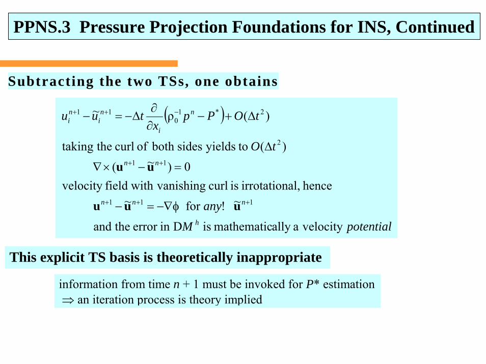
T h eta - im pl ic i t T S i s m ore app ropr ia te , hen ce

)()1(:TS )(

1

1 θ

+

+ Δ+⎟⎟⎠

⎞⎜⎜⎝

⎛∂∂

θ−+∂∂

θΔ=− f

n

i

n

ini

ni tO

tu

tutuu

substituting INS DP yields

)(ˆReGr

ρ1

Re1)(

)1(

ˆReGr

ρ1

Re1)(

:TS

22

0

1

20

1

tOgxp

xu

xxuu

t

gxp

xu

xxuu

tuu

n

iij

i

jj

ij

n

iij

i

jj

ijnini

Δ+⎥⎥⎦

⎤

⎢⎢⎣

⎡Θ+

∂∂

+⎟⎟⎠

⎞⎜⎜⎝

⎛

∂∂

∂∂

−∂

∂Δθ−−

⎥⎥⎦

⎤

⎢⎢⎣

⎡Θ+

∂∂

+⎟⎟⎠

⎞⎜⎜⎝

⎛

∂∂

∂∂

−∂

∂Δθ−=−

+

+

Repeating this TS using guessed pressure P* at time n+1 produces 1

*

+niu

!)(:note

)(Re1

Re1

ˆ)(ReGr)ρ()(

)(:TSsngsubstracti

1*

)(

1

*

1*

21

0*

1

**

1*

0uu ≠−×∇

Δ+⎥⎥⎦

⎤

⎢⎢⎣

⎡⎟⎟⎠

⎞⎜⎜⎝

⎛

∂∂

⎟⎠⎞

⎜⎝⎛−⎟

⎟⎠

⎞⎜⎜⎝

⎛

∂∂

∂∂

Δθ+

Θ−Θ+⎥⎦

⎤⎢⎣

⎡∂−∂

Δθ+⎥⎥⎦

⎤

⎢⎢⎣

⎡

∂∂

−∂∂

Δθ=−

+

θ

+

+

++

+

n

f

nj

i

j

i

j

inninj

ij

j

ijnii

tOxu

xu

xt

gx

pPtxuu

xuutuu


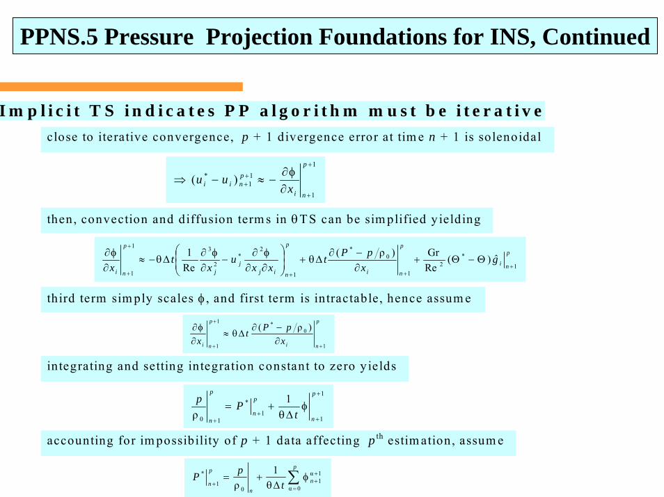
I m p l i c i t T S i n d i c a t e s P P a l g o r i t h m m u s t b e i t e r a t i v e

close to iterative convergence, p + 1 divergence error at tim e n + 1 is solenoidal

1

1

11

* )(+

+

++ ∂

φ∂−≈−⇒

p

ni

pnii x

uu

then, convection and diffusion term s in θT S can be sim plified y ielding

p

ni

p

ni

p

nijj

j

p

ni

gx

pPtxx

ux

tx 1

*2

1

0*

1

2*

2

31

1

ˆ)(ReGr)ρ(

Re1

+++

+

+

Θ−Θ+∂−∂

Δθ+⎟⎟⎠

⎞⎜⎜⎝

⎛

∂∂φ∂

−∂φ∂

Δθ−≈∂φ∂

third term sim ply scales φ , and first term is intractable, hence assum e p

ni

p

ni xpPt

x1

0*1

1

)ρ(

+

+

+∂−∂

Δθ≈∂φ∂

integrating and setting integration constant to zero y ields

1

11

*

10

1ρ

+

++

+

φΔθ

+=p

n

p

n

p

nt

Pp

accounting for im possibility of p + 1 data affecting p th estim ation, assum e

∑=

+++

φΔθ

+=p

nn

p

n tpP

0α

1α1

01

* 1ρ


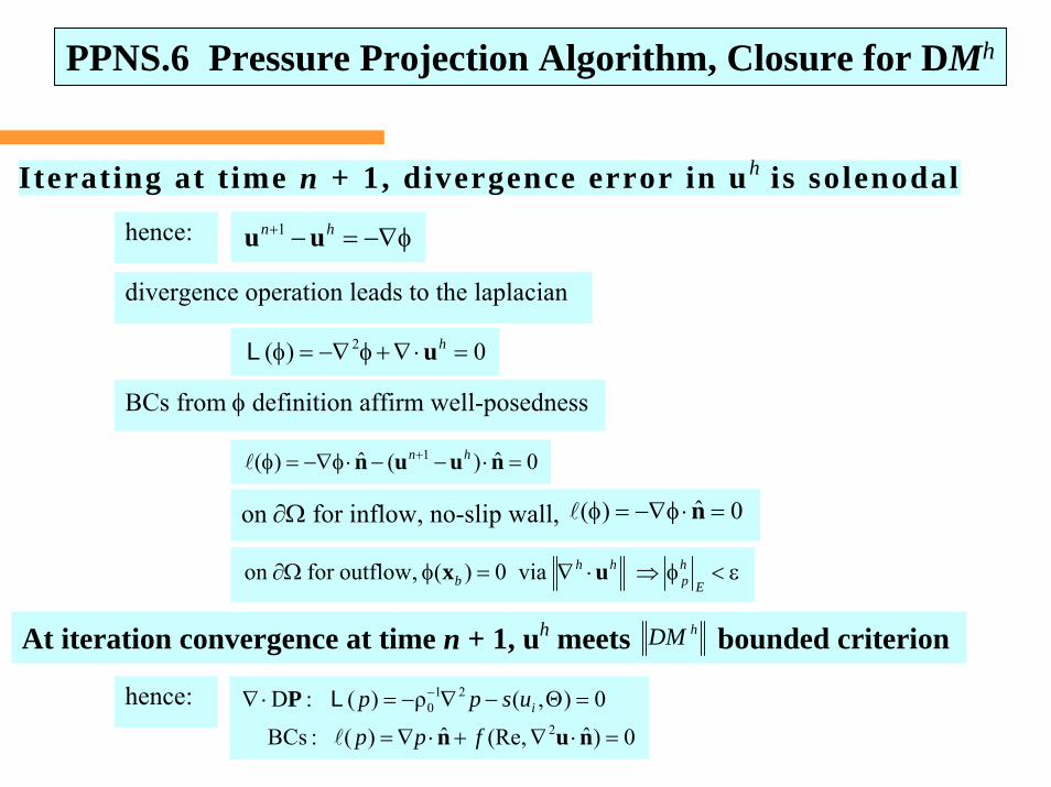
Iterating at t ime n + 1, divergence error in uh is solenodal

hence: φ−∇=−+ hn uu 1

divergence operation leads to the laplacian

0)( 2 =⋅∇+φ−∇=φ huL

BCs from φ definition affirm well-posedness

0ˆ)(ˆ)( 1 =⋅−−⋅φ−∇=φ + nuun hn

on ∂Ω for inflow, no-slip wall, 0ˆ)( =⋅φ−∇=φ n

ε<φ⇒⋅∇=φΩ∂E

hp

hhb ux via0)(,outflowforon

At iteration convergence at time n + 1, uh meets hDM bounded criterion

hence: 0)ˆ(Re,ˆ)(:BCs

0),(ρ)(:D2

210

=⋅∇+⋅∇=

=Θ−∇−=⋅∇ −

nun

P

fpp

uspp iL

PPNS.6 Pressure Projection Algorithm, Closure for DMh

PPNS.7 Pressure Projection INS PDE + BC System

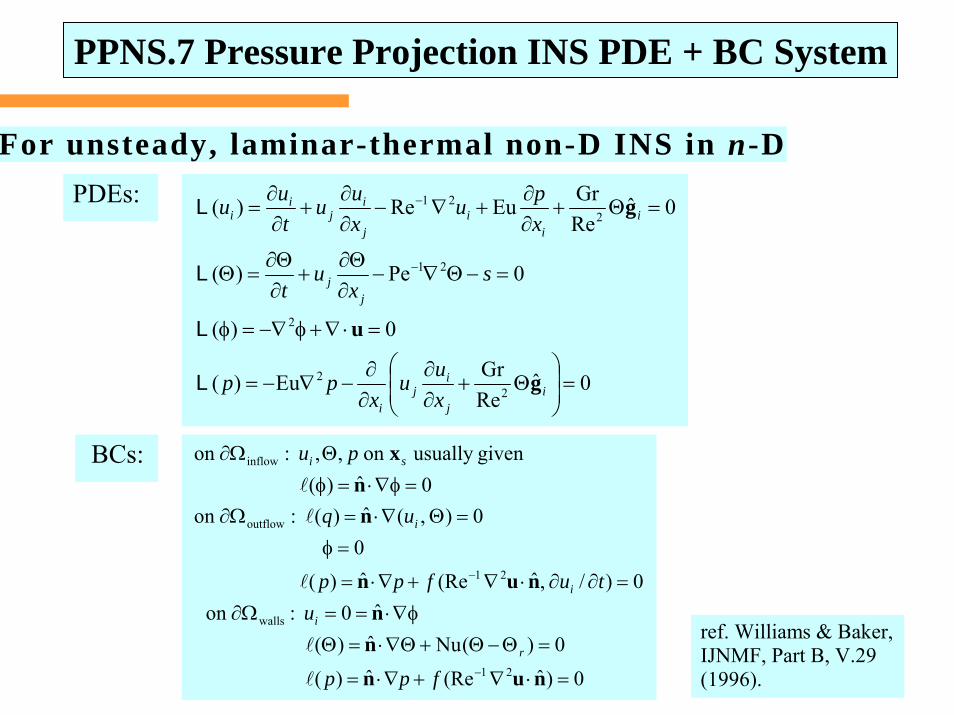
For unsteady, laminar-thermal non-D INS in n-D

PDEs:

0ˆReGrEu)(

0)(

0Pe)(

0ˆReGrEuRe)(

22

2

21

221

=⎟⎟⎠

⎞⎜⎜⎝

⎛Θ+

∂∂

∂∂

−∇−=

=⋅∇+φ−∇=φ

=−Θ∇−∂Θ∂

+∂Θ∂

=Θ

=Θ+∂∂

+∇−∂∂

+∂∂

=

−

−

ij

ij

i

jj

ii

ij

ij

ii

xuu

xpp

sx

ut

xpu

xuu

tuu

g

u

g

L

L

L

L

BCs:

0)ˆ(Reˆ)(

0)(Nuˆ)(ˆ0:on

0)/,ˆ(Reˆ)(0

0),(ˆ)(:on0ˆ)(

givenusuallyon,,:on

21

walls

21

outflow

inflow

=⋅∇+∇⋅=

=Θ−Θ+Θ∇⋅=Θφ∇⋅==Ω∂

=∂∂⋅∇+∇⋅=

=φ=Θ∇⋅=Ω∂

=φ∇⋅=φΘΩ∂

−

−

nun

nn

nun

nn

x

fpp

utufpp

uq

pu

r

i

i

i

si

ref. Williams & Baker,IJNMF, Part B, V.29 (1996).

PPNS.8 GWSh + θTS for Pressure Projection INS

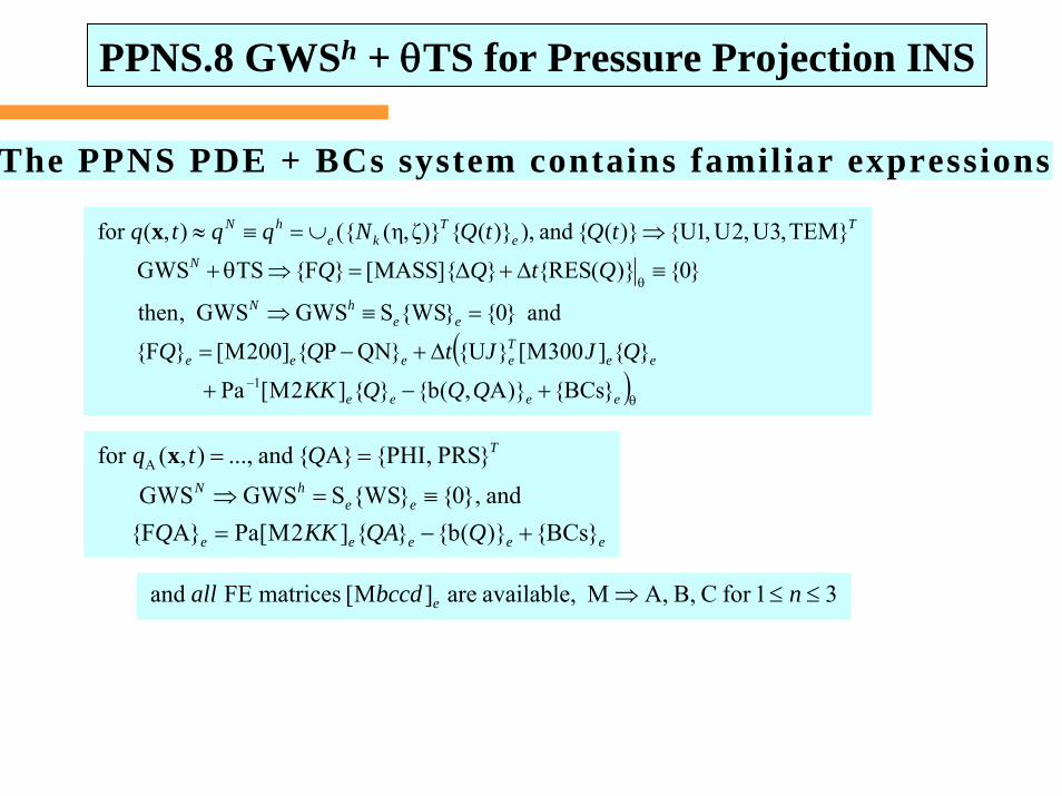
The PPNS PDE + BCs system contains familiar expressions

()θ−

θ

+−+

Δ+−=

=≡⇒

≡Δ+Δ=⇒θ+

⇒∪=≡≈

eeee

eeTeeee

eehN

N

Te

Tke

hN

QQQKK

QJJtQQ

QtQQ

tQtQNqqtq

}BCs{)}A,(b{}{]2M[Pa

}{]300M[}U{}QNP{]200M[}F{

and}0{}WS{SGWSGWS,then

}0{)}(RES{}]{MASS[}F{TSGWS

}TEM,3U,2U,1U{)}({and),)}({)}ζ,η(({),(for

1

x

eeeee

eehN

T

QQAKKQ

Qtq

}BCs{)}(b{}{]2M[Pa}AF{and},0{}WS{SGWSGWS

}PRS,PHI{}A{and...,),(for A

+−=≡=⇒

==x

31forCB,A,M available,are]M[matricesFE and ≤≤⇒ nbccdall e

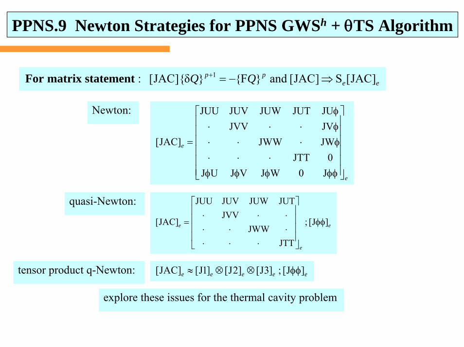
PPNS.9 Newton Strategies for PPNS GWSh + θTS Algorithm

eepp QQ ]JAC[S]JAC[and}F{}δ]{JAC[: 1 ⇒−=+statementmatrixFor

Newton:

e

e

⎥⎥⎥⎥⎥⎥

⎦

⎤

⎢⎢⎢⎢⎢⎢

⎣

⎡

φφ0φφφ⋅⋅⋅

φ⋅⋅⋅φ⋅⋅⋅φ

=

JWJVJUJ0JTT

JWJWWJVJVVJUJUTJUWJUVJUU

]JAC[

quasi-Newton:

e

e

e ]J[;

JTTJWW

JVVJUTJUWJUVJUU

]JAC[ φφ

⎥⎥⎥⎥

⎦

⎤

⎢⎢⎢⎢

⎣

⎡

⋅⋅⋅⋅⋅⋅⋅⋅⋅

=

tensor product q-Newton: eeeee ]J[;]3J[]2J[]1J[]JAC[ φφ⊗⊗≈

explore these issues for the thermal cavity problem

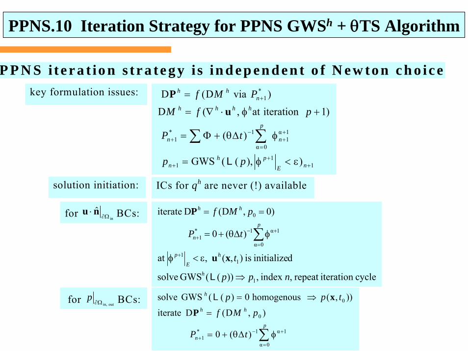
PPNS.10 Iteration Strategy for PPNS GWSh + θTS Algorithm

P P N S i t e r a t io n s t r a te g y i s in d e p e n d e n t o f N e w to n c h o ic e

key formulation issues:

11

1

0

1α1

1*1

*1

)),((GWS

)(

)1iterationat,(D

)viaD(D

++

+

=

++

−+

+

ε<φ=

φΔθ+Φ=

+φ⋅∇=

=

∑∑

nE

phn

p

nn

hhhhn

hh

pp

tP

pfM

PMf

Lα

u

P

solution initiation: ICs for qh are never (!) available

for in

ˆΩ∂

⋅nu BCs:

cycleiterationrepeat,index,))((GWSsolve

dinitializeis),(,at

)(0

)0,D(Diterate

1

11

0α

1α1*1

0

npp

t

tP

pMf

h

h

E

p

p

n

hh

⇒

ε<φ

φΔθ+=

==

+

=

+−+ ∑

L

xu

P

∑=

+−+ φΔθ+=

=

⇒=

p

n

hh

h

tP

pMf

tpp

0α

1α1*1

0

0

)(0

),D(Diterate

)),(homogenous0)((GWSsolve

P

xL for outin,Ω∂

p BCs:

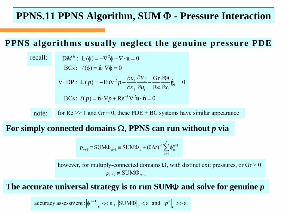
PPNS.11 PPNS Algorithm, SUM Φ - Pressure Interaction

PPNS algorithms usually neglect the genuine pressure PDE

recall:

0ˆReˆ)(:BCs

0ˆReGrEu)(:D

0ˆ)(:BCs0)(:D

21

2

2

=⋅∇+∇⋅=

=∂Θ∂

−∂

∂

∂∂

−∇−=⋅∇

=φ∇⋅=φ=⋅∇+φ−∇=φ

− nun

gP

nu

pp

xuu

xupp

M

iii

j

j

i

h

L

L

note: for Re >> 1 and Gr = 0, these PDE + BC systems have similar appearance

∑=

+−++ φΔθ+Φ≡Φ≅

p

nnnn tp1α

1α111 )(SUMSUM

however, for multiply-connected domains Ω, with distinct exit pressures, or Gr > 0 pn+1 ≠ SUMΦn+1

The accurate universal strategy is to run SUMΦ and solve for genuine p

ε>>ε<Φε<<φ +

E

hEE

p pandSUM,:assessmentaccuracy 1

For simply connected domains Ω, PPNS can run without p via

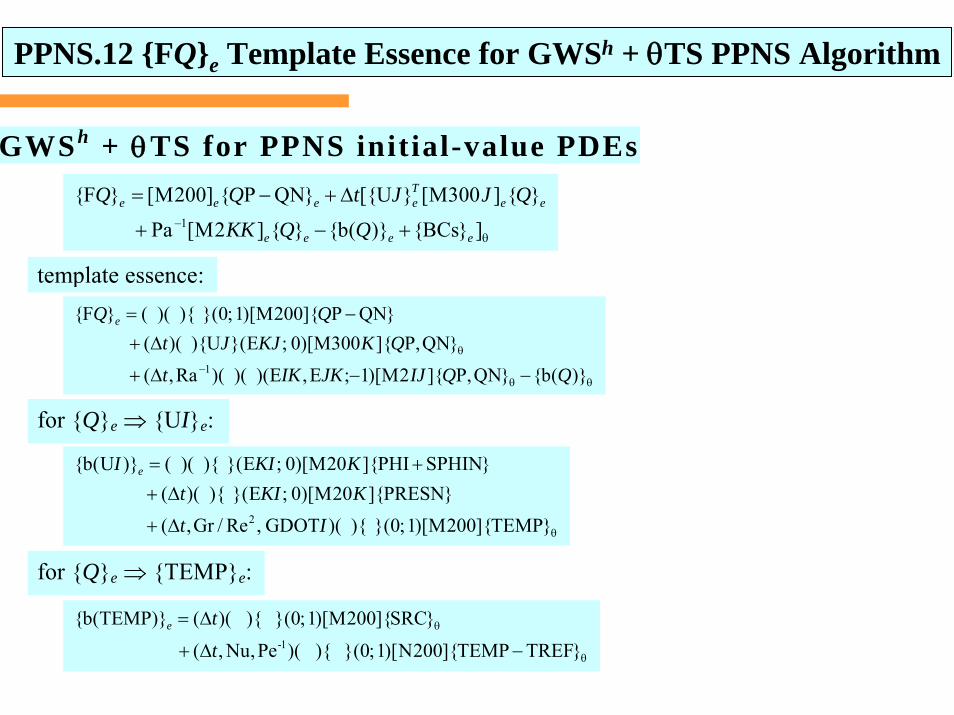
PPNS.12 {FQ}e Template Essence for GWSh + θTS PPNS Algorithm

GWSh + θTS for PPNS initial-value PDEs

θ− +−+

Δ+−=

]}BCs{)}(b{}{]2M[Pa

}{]300M[}U[{}QNP{]200M[}F{1

eeee

eeTeeee

QQKK

QJJtQQ

template essence:

θθ−

θ

−−Δ+

Δ+−=

)}(b{}QN,P]{2M)[1;E,E)()()(Ra,(

}QN,P]{300M)[0;E}(U){)((}QNP]{200M)[1;0}(){)((}F{

1 QQIJJKIKt

QKKJJtQQ e

for {Q}e ⇒ {UI}e:

θΔ+

Δ++=

}TEMP]{200M)[1;0}(){)(GDOT,Re/Gr,(}PRESN]{20M)[0;E}(){)((

}SPHINPHI]{20M)[0;E}(){)(()}U(b{

2 ItKKIt

KKII e

for {Q}e ⇒ {TEMP}e:

θ

θ

−Δ+

Δ=

}TREFTEMP]{200N)[1;0}(){)(Pe,Nu,(

}SRC]{200M)[1;0}(){)(()}TEMP(b{1-t

te

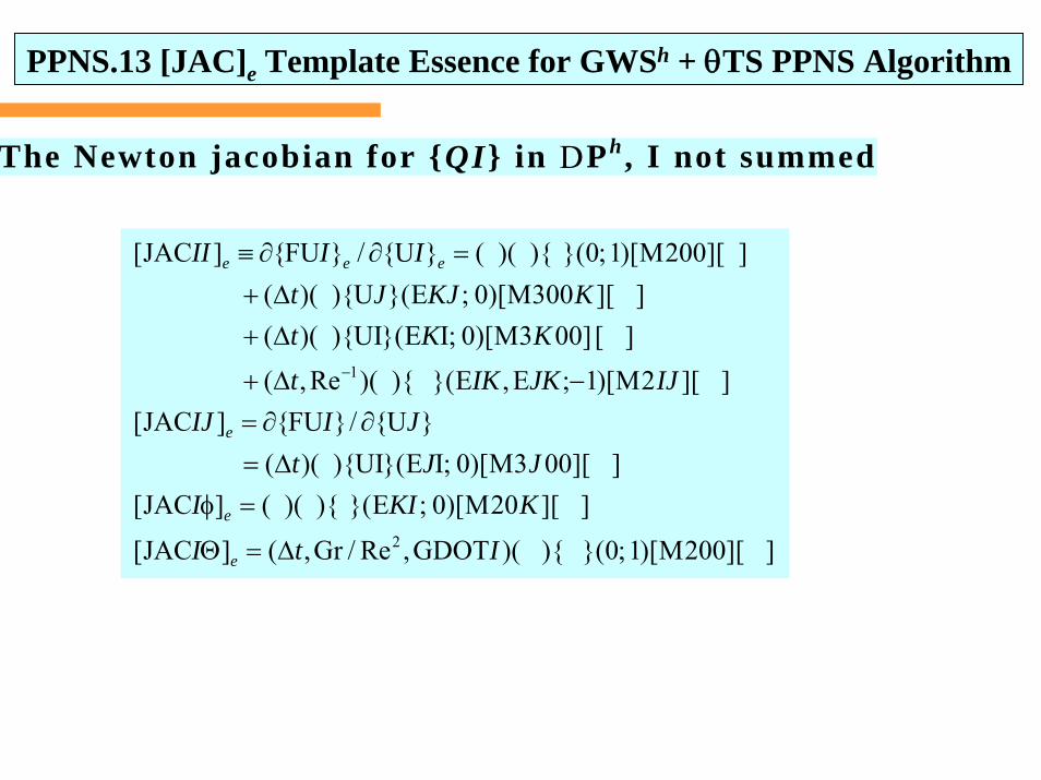
PPNS.13 [JAC]e Template Essence for GWSh + θTS PPNS Algorithm

The Newton jacobian for {QI} in DPh , I not summed

]][200M)[1;0}(){)(GDOT,Re/Gr,(]JAC[

]][20M)[0;E}(){)((]JAC[]][003M)[0;IE}(UI){)((

}U{/}FU{]JAC[]][2M)[1;E,E}(){)(Re,(

][]003M)[0;IE}(UI){)((]][300M)[0;E}(U){)((

]][200M)[1;0}(){)((}U{/}FU{]JAC[

2

1

ItI

KKIIJJt

JIIJIJJKIKt

KKtKJKJt

IIII

e

e

e

eee

Δ=Θ

=φΔ=

∂∂=−Δ+

Δ+Δ+

=∂∂≡

−

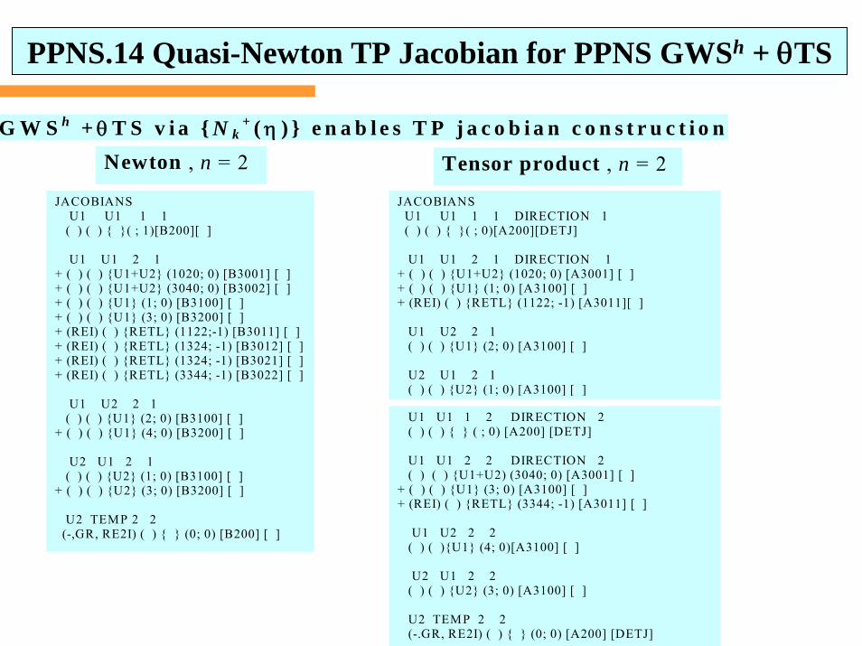
PPNS.14 Quasi-Newton TP Jacobian for PPNS GWSh + θTS

G W S h + θT S v i a { N k+ (η ) } e n a b l e s T P j a c o b i a n c o n s t r u c t i o n

Newton , n = 2 Tensor product , n = 2

JACOBIANS U1 U1 1 1 ( ) ( ) { }( ; 1)[B200][ ] U1 U1 2 1 + ( ) ( ) {U1+U2} (1020; 0) [B3001] [ ] + ( ) ( ) {U1+U2} (3040; 0) [B3002] [ ] + ( ) ( ) {U1} (1; 0) [B3100] [ ] + ( ) ( ) {U1} (3; 0) [B3200] [ ] + (REI) ( ) {RETL} (1122;-1) [B3011] [ ]+ (REI) ( ) {RETL} (1324; -1) [B3012] [ ]+ (REI) ( ) {RETL} (1324; -1) [B3021] [ ]+ (REI) ( ) {RETL} (3344; -1) [B3022] [ ] U1 U2 2 1 ( ) ( ) {U1} (2; 0) [B3100] [ ] + ( ) ( ) {U1} (4; 0) [B3200] [ ] U2 U1 2 1 ( ) ( ) {U2} (1; 0) [B3100] [ ] + ( ) ( ) {U2} (3; 0) [B3200] [ ] U2 TEMP 2 2 (-,GR, RE2I) ( ) { } (0; 0) [B200] [ ]

JACOBIANS U1 U1 1 1 DIRECTION 1 ( ) ( ) { }( ; 0)[A200][DETJ] U1 U1 2 1 DIRECTION 1 + ( ) ( ) {U1+U2} (1020; 0) [A3001] [ ] + ( ) ( ) {U1} (1; 0) [A3100] [ ] + (REI) ( ) {RETL} (1122; -1) [A3011][ ] U1 U2 2 1 ( ) ( ) {U1} (2; 0) [A3100] [ ] U2 U1 2 1 ( ) ( ) {U2} (1; 0) [A3100] [ ]

U1 U1 1 2 DIRECTION 2 ( ) ( ) { } ( ; 0) [A200] [DETJ] U1 U1 2 2 DIRECTION 2 ( ) ( ) {U1+U2) (3040; 0) [A3001] [ ] + ( ) ( ) {U1} (3; 0) [A3100] [ ] + (REI) ( ) {RETL} (3344; -1) [A3011] [ ] U1 U2 2 2 ( ) ( ){U1} (4; 0)[A3100] [ ] U2 U1 2 2 ( ) ( ) {U2} (3; 0) [A3100] [ ] U2 TEMP 2 2 (-.GR, RE2I) ( ) { } (0; 0) [A200] [DETJ]

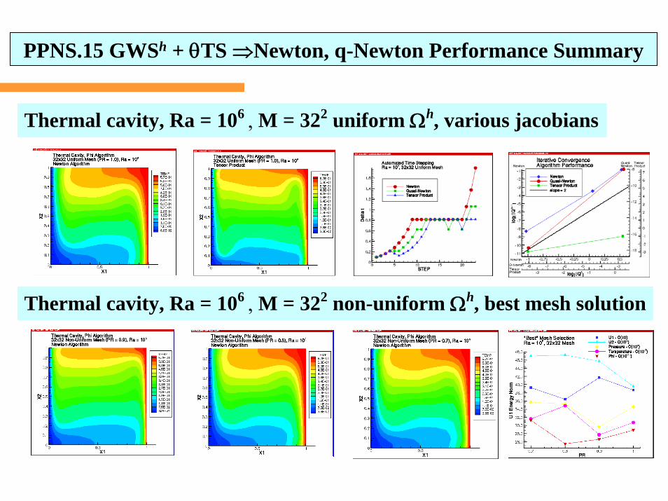
Thermal cavity, Ra = 106 , M = 322 non-uniform Ωh, best mesh solution

Thermal cavity, Ra = 106 , M = 322 uniform Ωh, various jacobians

PPNS.15 GWSh + θTS ⇒Newton, q-Newton Performance Summary

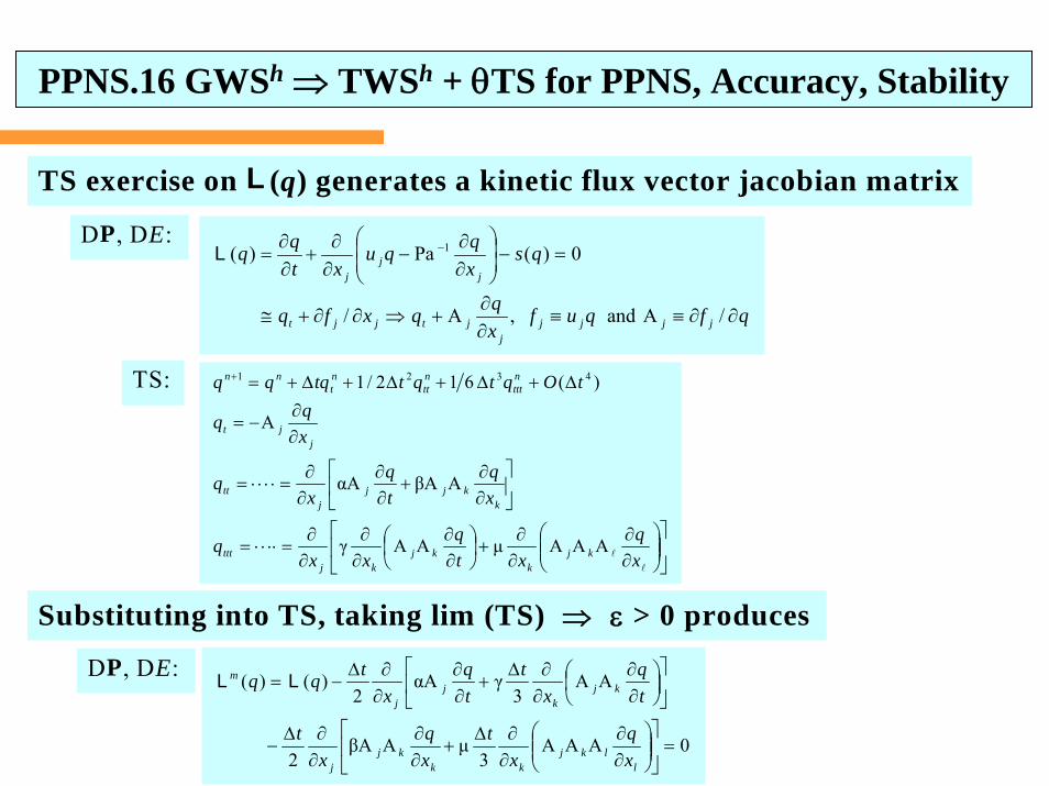
TS exercise on L (q) generates a kinetic flux vector jacobian matrix

DP, DE:

qfqufxqqxfq

qsxqqu

xtqq

jjjjj

jtjjt

jj

j

∂∂≡≡∂∂

+⇒∂∂+≅

=−⎟⎟⎠

⎞⎜⎜⎝

⎛

∂∂

−∂∂

+∂∂

= −

/Aand,A/

0)(Pa)( 1L

TS:

⎥⎦

⎤⎢⎣

⎡⎟⎟⎠

⎞⎜⎜⎝

⎛∂∂

∂∂

+⎟⎠⎞

⎜⎝⎛

∂∂

∂∂

∂∂

=⋅⋅⋅⋅=

⎥⎦

⎤⎢⎣

⎡∂∂

+∂∂

∂∂

=⋅⋅⋅⋅=

∂∂

−=

Δ+Δ+Δ+Δ+=+

xq

xtq

xxq

xq

tq

xq

xqq

tOqtqttqqq

kjk

kjkj

ttt

kkjj

jtt

jjt

nttt

ntt

nt

nn

AAAμAAγ

AβAαA

A

)(612/1 4321

Substituting into TS, taking lim (TS) ⇒ ε > 0 produces

DP, DE:

0AAA3

μAβA2

AA3

γαA2

)()(

=⎥⎦

⎤⎢⎣

⎡⎟⎟⎠

⎞⎜⎜⎝

⎛∂∂

∂∂Δ

+∂∂

∂∂Δ

−

⎥⎦

⎤⎢⎣

⎡⎟⎠⎞

⎜⎝⎛

∂∂

∂∂Δ

+∂∂

∂∂Δ

−=

llkj

kkkj

j

kjk

jj

m

xq

xt

xq

xt

tq

xt

tq

xtqq LL

PPNS.16 GWSh ⇒ TWSh + θTS for PPNS, Accuracy, Stability

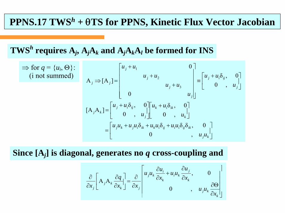
TWSh requires Aj, AjAk and AjAkAl be formed for INS

⇒ for q = {ui, Θ}: (i not summed)

⎥⎦

⎤⎢⎣

⎡ +++=

⎥⎦

⎤⎢⎣

⎡ +⎥⎦

⎤⎢⎣

⎡ +=

⎥⎦

⎤⎢⎣

⎡ +≡

⎥⎥⎥⎥⎥

⎦

⎤

⎢⎢⎢⎢⎢

⎣

⎡

++

+

=⇒

kj

kjjkkjkj

k

kk

j

jjkj

j

jj

j

j

j

j

jj

uuuuuuuuuu

uuu

uuu

uuu

uuu

uuuu

,00,δδδδ

,00,δ

,00,δ

]AA[

,00,δ

0

0

]A[A

iiiiiiii

iiii

ii

3

2

1

Since [Aj] is diagonal, generates no q cross-coupling and

⎥⎥⎥⎥

⎦

⎤

⎢⎢⎢⎢

⎣

⎡

∂Θ∂

∂

∂+

∂∂

∂∂

=⎥⎦

⎤⎢⎣

⎡∂∂

∂∂

kkj

k

jki

k

ikj

jkkj

j

xuu

xu

uuxuuu

xxq

x ,0

0,AA

PPNS.17 TWSh + θTS for PPNS, Kinetic Flux Vector Jacobian

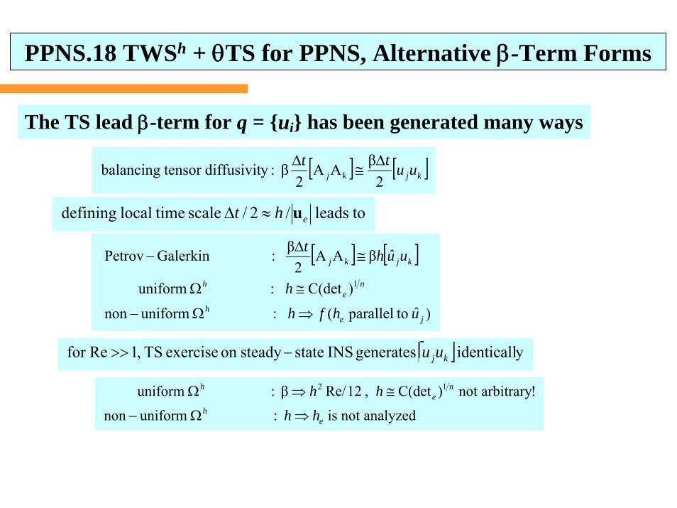
The TS lead β-term for q = {ui} has been generated many ways

[ ] [ ]kjkj uutt2βAA

2β:ydiffusivittensorbalancing Δ

≅Δ

toleads/2/scaletimelocaldefining eht u≈Δ

[ ] [ ]

)ˆtoparallel(:uniformnon

)(detC:uniform

ˆβAA2β:GalerkinPetrov

1

jeh

ne

h

kjkj

uhfh

h

uuht

⇒Ω−

≅Ω

≅Δ

−

[ ] yidenticallgeneratesINSstatesteadyonexerciseTS,1Refor kjuu−>>

analyzednotis:uniformnon

!arbitrarynot)(detC,12Re/β:uniform 12

eh

ne

h

hh

hh

⇒Ω−

≅⇒Ω

PPNS.18 TWSh + θTS for PPNS, Alternative β-Term Forms

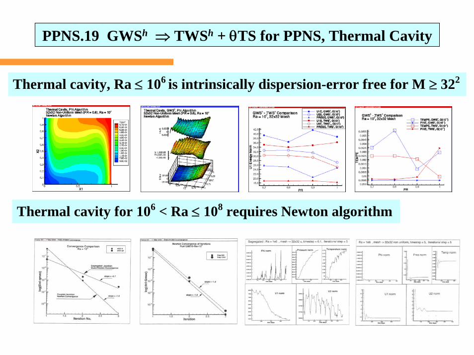
Thermal cavity for 106 < Ra ≤ 108 requires Newton algorithm

Thermal cavity, Ra ≤ 106 is intrinsically dispersion-error free for M ≥ 322

PPNS.19 GWSh ⇒ TWSh + θTS for PPNS, Thermal Cavity

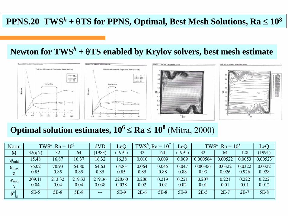
Optimal solution estimates, 106 ≤ Ra ≤ 108 (Mitra, 2000)

Newton for TWSh + θTS enabled by Krylov solvers, best mesh estimate

Norm TWSh, Ra = 106 dVD LeQ TWSh, Ra = 107 LeQ TWSh, Ra = 108 LeQ M 32(qN) 32 64 (1983) (1991) 32 64 (1991) 32 64 128 (1991) ψmid 15.48 16.87 16.37 16.32 16.38 0.010 0.009 0.009 0.000564 0.00522 0.0053 0.00523

umax z

76.02 0.85

70.93 0.85

64.80 0.85

64.63 0.85

64.83 0.85

0.064 0.85

0.045 0.88

0.047 0.88

0.00306 0.93

0.0322 0.926

0.0322 0.926

0.0322 0.928

wmax x

209.11 0.04

213.32 0.04

219.33 0.04

219.36 0.038

220.60 0.038

0.206 0.02

0.219 0.02

0.221 0.02

0.207 0.01

0.221 0.01

0.222 0.01

0.222 0.012

E

hφ 5E-5 5E-8 5E-8 --- 5E-9 2E-6 5E-8 5E-9 2E-5 2E-7 2E-7 5E-8

PPNS.20 TWSh + θTS for PPNS, Optimal, Best Mesh Solutions, Ra ≤ 108

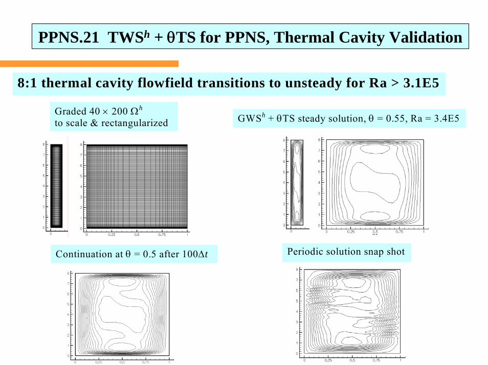
8:1 thermal cavity flowfield transitions to unsteady for Ra > 3.1E5

Graded 40 × 200 Ωh to scale & rectangularized GWSh + θTS steady solution, θ = 0.55, Ra = 3.4E5

Continuation at θ = 0.5 after 100Δt Periodic solution snap shot

PPNS.21 TWSh + θTS for PPNS, Thermal Cavity Validation

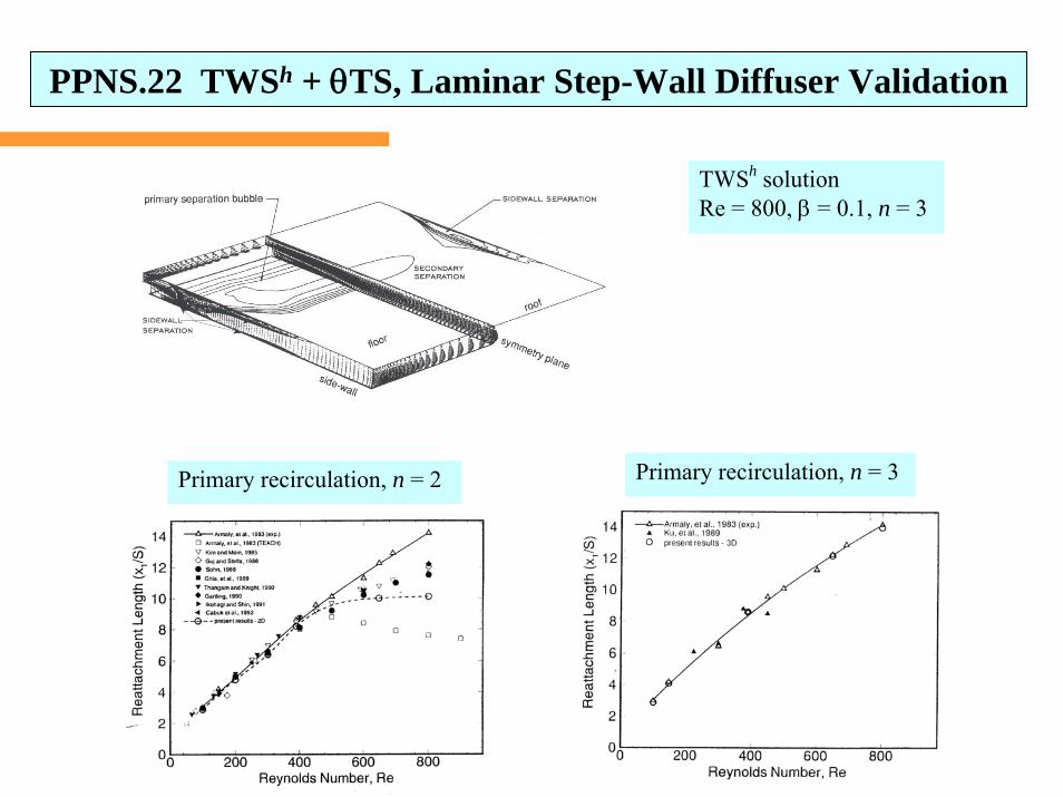
TWSh solution Re = 800, β = 0.1, n = 3

Primary recirculation, n = 2 Primary recirculation, n = 3

PPNS.22 TWSh + θTS, Laminar Step-Wall Diffuser Validation

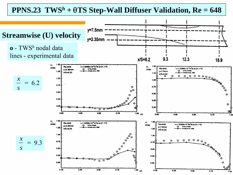
o - TWSh nodal data lines - experimental data

xs

= 6.2

xs

= 9.3

Streamwise (U) velocity

PPNS.23 TWSh + θTS Step-Wall Diffuser Validation, Re = 648

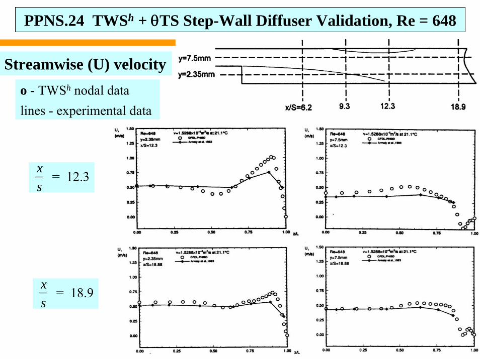
o - TWSh nodal datalines - experimental data

xs

= 12.3

xs

= 18.9

Streamwise (U) velocity

PPNS.24 TWSh + θTS Step-Wall Diffuser Validation, Re = 648

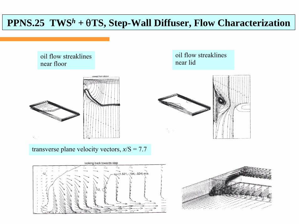
oil flow streaklinesnear floor

oil flow streaklines near lid

transverse plane velocity vectors, x/S = 7.7

PPNS.25 TWSh + θTS, Step-Wall Diffuser, Flow Characterization

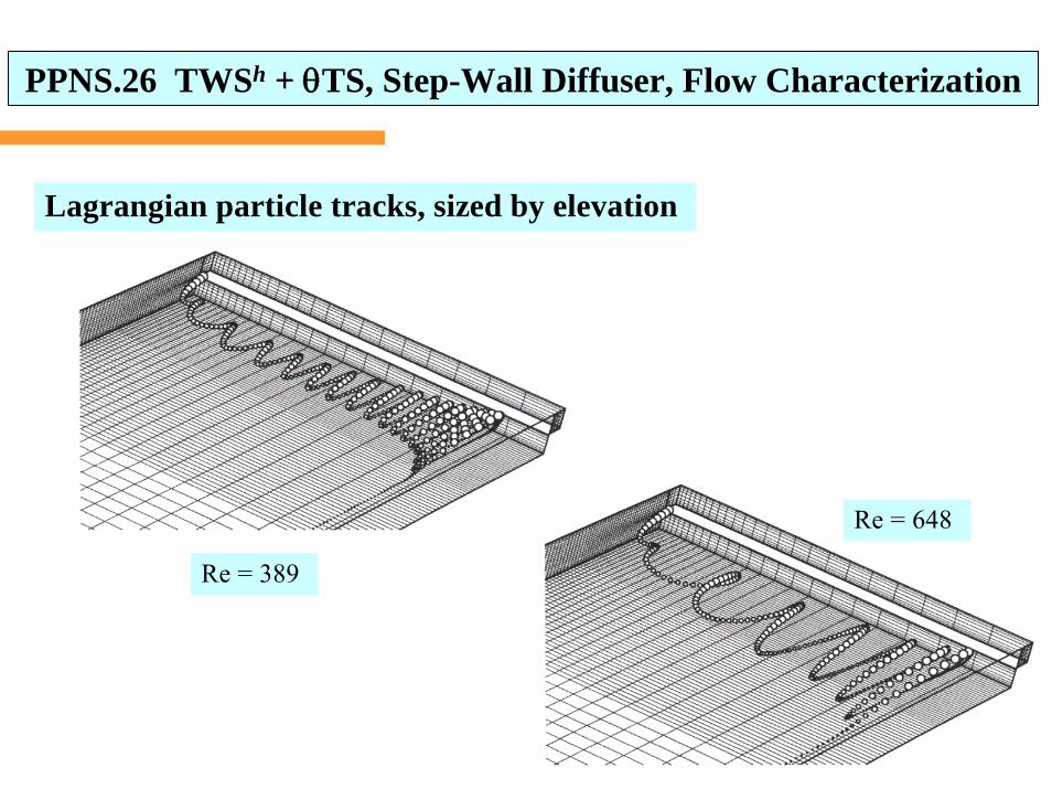
Lagrangian particle tracks, sized by elevation

Re = 389

Re = 648

PPNS.26 TWSh + θTS, Step-Wall Diffuser, Flow Characterization

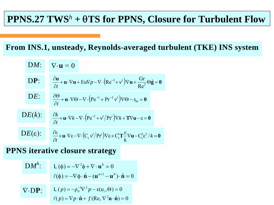
From INS.1, unsteady, Reynolds-averaged turbulent (TKE) INS system

DM: ∇⋅u = 0

DP: ( ) 0guuuu=Θ+∇+⋅∇−∇+∇⋅+

∂∂ − ˆ

ReGrReEu 2

1 tvpt

DE: ( ) 0u =−Θ∇+⋅∇−Θ∇⋅+∂Θ∂

Θ−− sv

tt11 PrPe

DE(k):

DE(ε):

( ) 0uTu =−∇+∇+⋅∇−∇⋅+∂∂ − εPrPe 1 kvk

tk tt

( ) 0uTu =−∇+∇⋅∇−∇⋅+∂∂ k

kv

ttt /εCεCεPrCεε 22

ε1εε

PPNS iterative closure strategy

0ˆ)(ˆ)(0)(

1

2

=⋅−−⋅φ−∇=φ

=⋅∇+φ−∇=φ+ nuun

uhn

hLDMh:

∇⋅DP: 0)ˆ(Re,ˆ)(

0),(ρ)(2

210

=⋅∇+⋅∇=

=Θ−∇−= −

nun fpp

uspp iL

PPNS.27 TWSh + θTS for PPNS, Closure for Turbulent Flow

u

n

y+

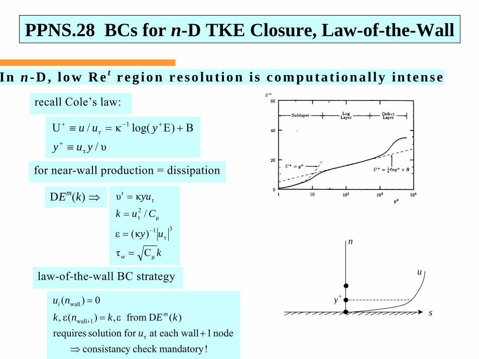
In n -D , low R e t r eg io n reso lu t io n i s com puta t iona l ly in tense

υ/

B)Elog(κ/U

τ

1

yuy

yuu

≡

+=≡+

+−+τ

recall Cole’s law:

k

uy

Cuk

yu

w

t

μ

3τ

1

μ2τ

τ

Cτ

)κ(

/

κυ

=

=ε

=

=

−

DEm(k) ⇒

for near-wall production = dissipation

law-of-the-wall BC strategy

!mandatorycheckyconsistancnode1walleachatforsolutionrequires

)(Dfrom,)(,

0)(

τ

1wall

wall

⇒+

ε=ε

=

+

ukEknk

num

is

PPNS.28 BCs for n-D TKE Closure, Law-of-the-Wall

+u BEynuu ≡⎟⎟⎠

⎞⎜⎜⎝

⎛ + + 1 = / κτ

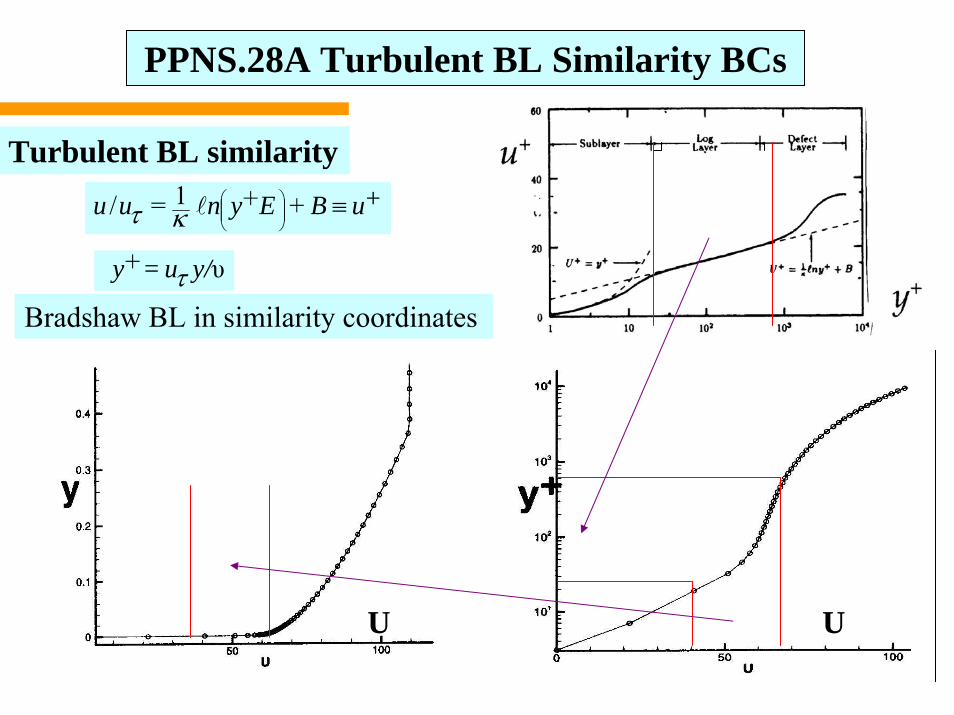
Bradshaw BL in similarity coordinates

U

y/u =y υ+ τ

U

PPNS.28A Turbulent BL Similarity BCs

Turbulent BL similarity

TWSh + θTS for qh ⇒ {U1, U2, U3, T, PHI; K, EPS, TIJ: PRES}T

q-Newton [JAC]e :

e

eijijijij

ij

ij

e

]JPP[;TJT,EJT,KJT

JET,JEE,JEKJKT,JKE,JKK

;

J,0,WJ,VJ,UJ0,JTT,JTW,JTV,JTU

JW,JWT,JWW,JWV,JWUJV,0,JVW,JVV,JVUJU,0,JUW,JUV,JUU

⎥⎥⎥

⎦

⎤

⎢⎢⎢

⎣

⎡

⎥⎥⎥⎥⎥⎥

⎦

⎤

⎢⎢⎢⎢⎢⎢

⎣

⎡

φφφφφ

φφφ

note: for laminar flow yields genuine Newton ⇔ Krylov solver

Iteration stabilization accrues to state variable update delay

loopiterationrestart}PRES{forsolve},2{},1{foreconvergencat

)}N1(2F{}2F{:}T,EPS,K{}2{for

)}N2(1F{}1F{:},T,U{}1{for

1+

==

=φ=

n

peeij

Te

pee

Te

QQ

QQQQ

QQQIQ

Template essence follows in aPSE file

PPNS.29 TWSh + θTS PPNS Algorithm q-Newton Template Essence

Laminar duct flow, Re/L = 1000: stability, φ, Σφ, pressure

GWSh, β = 0, u1h φh, E-05

TWSh, β = 0.2, u1h

Σφh, E-05 Pressure, E-04

φh, E-05 Σφh, E-05 Pressure, E-04

PPNS.30 GWSh ⇒ TWSh + θTS PPNS Algorithm, Performance of Theory

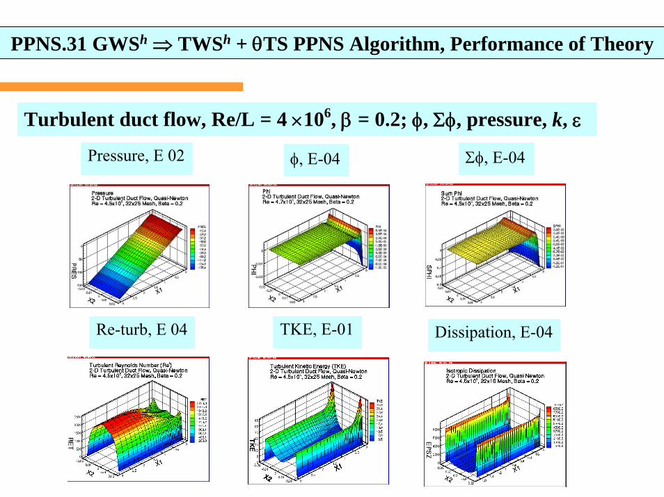
Turbulent duct flow, Re/L = 4 ×106, β = 0.2; φ, Σφ, pressure, k, ε

Pressure, E 02 φ, E-04 Σφ, E-04

Re-turb, E 04 TKE, E-01 Dissipation, E-04

PPNS.31 GWSh ⇒ TWSh + θTS PPNS Algorithm, Performance of Theory

RaNS + TKE turbulent entrance duct TWSh solution

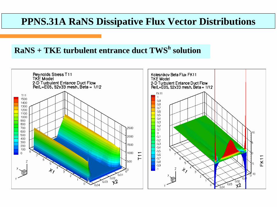
PPNS.31A RaNS Dissipative Flux Vector Distributions


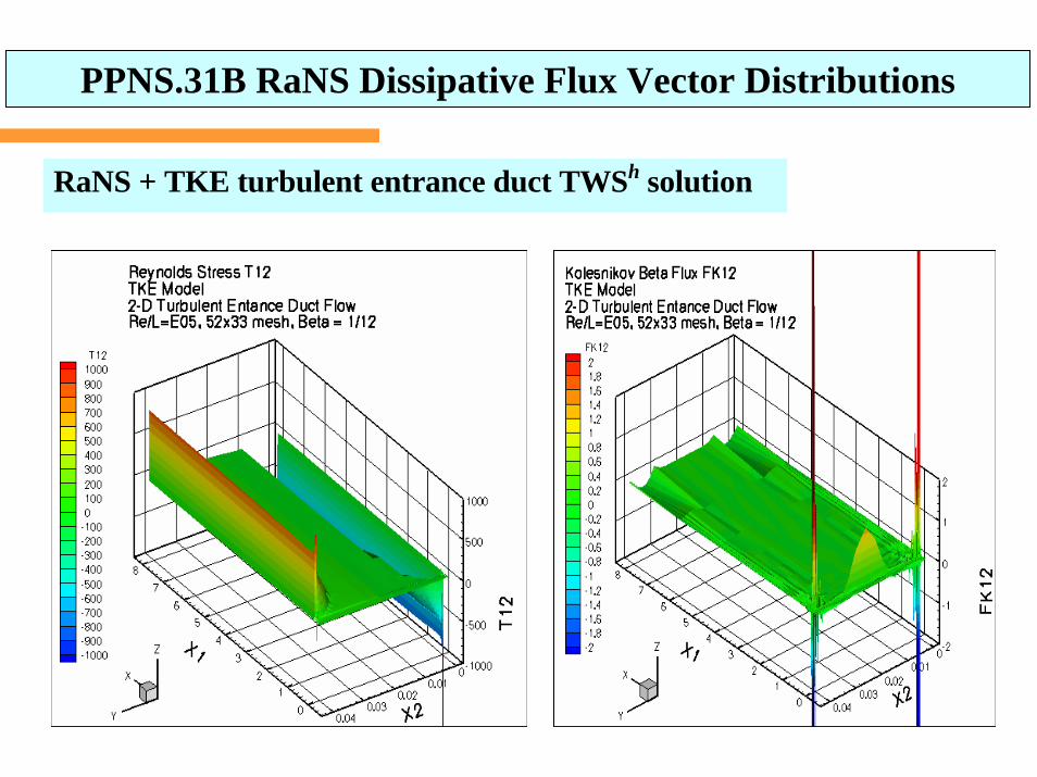
PPNS.31B RaNS Dissipative Flux Vector Distributions


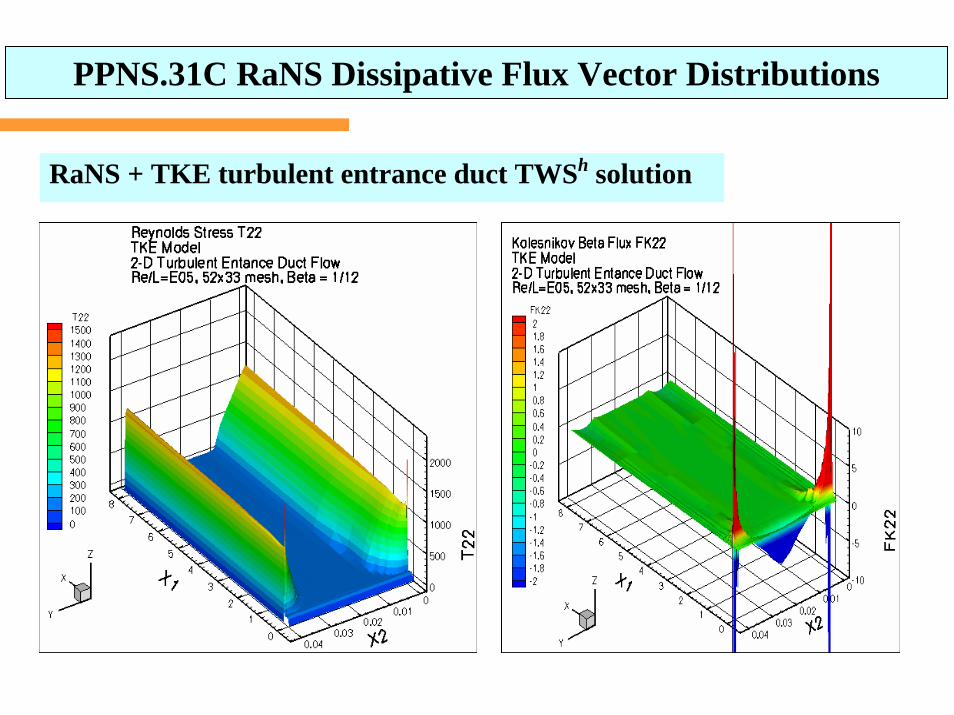
PPNS.31C RaNS Dissipative Flux Vector Distributions


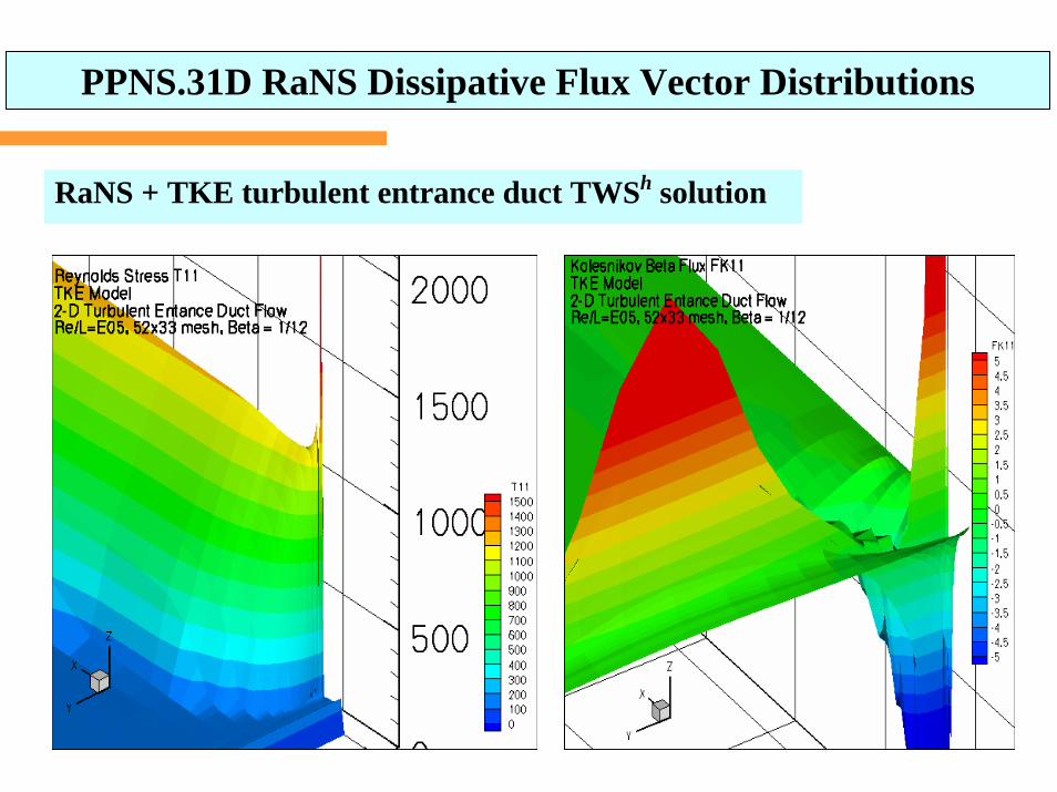
PPNS.31D RaNS Dissipative Flux Vector Distributions


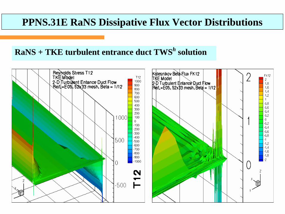
PPNS.31E RaNS Dissipative Flux Vector Distributions


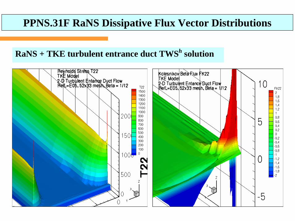
PPNS.31F RaNS Dissipative Flux Vector Distributions

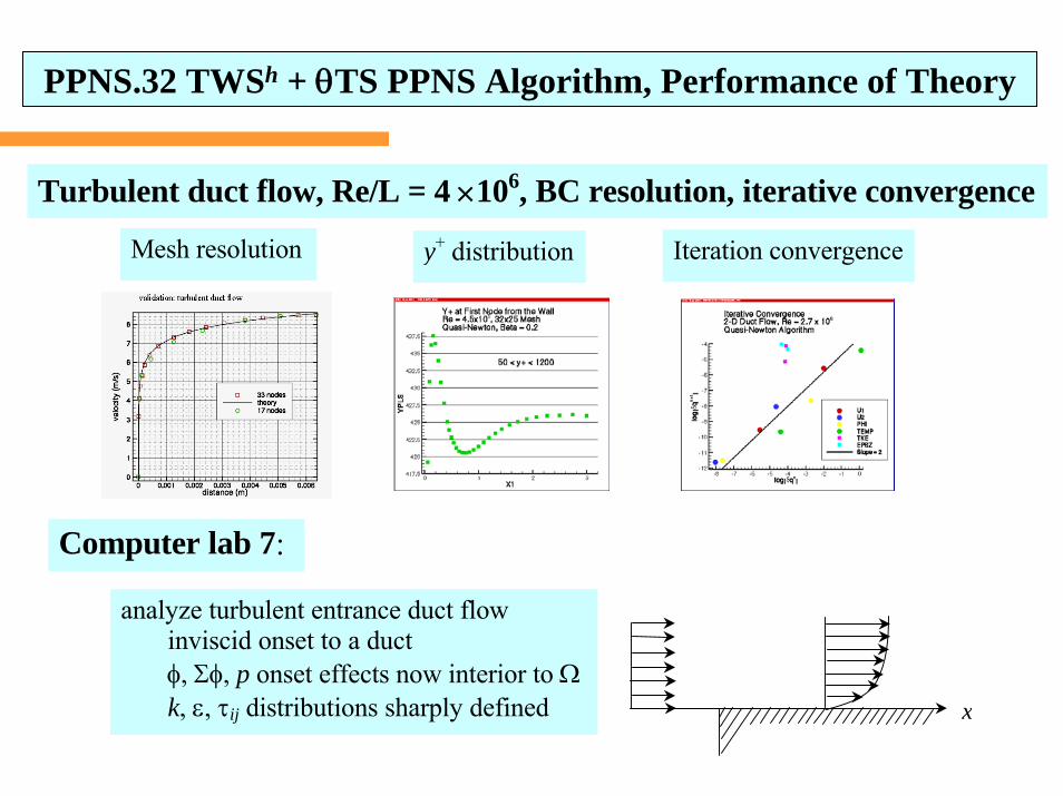
Turbulent duct flow, Re/L = 4 ×106, BC resolution, iterative convergence

Mesh resolution y+ distribution Iteration convergence

Computer lab 7:

analyze turbulent entrance duct flow inviscid onset to a duct φ, Σφ, p onset effects now interior to Ω k, ε, τij distributions sharply defined x

PPNS.32 TWSh + θTS PPNS Algorithm, Performance of Theory

flux

ΩPPNS ΩDEh

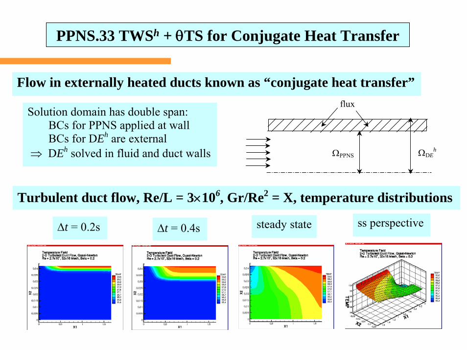
Flow in externally heated ducts known as “conjugate heat transfer”

Δt = 0.2s steady state ss perspective

Solution domain has double span: BCs for PPNS applied at wall BCs for DEh are external ⇒ DEh solved in fluid and duct walls

Turbulent duct flow, Re/L = 3×106, Gr/Re2 = X, temperature distributions

Δt = 0.4s

PPNS.33 TWSh + θTS for Conjugate Heat Transfer

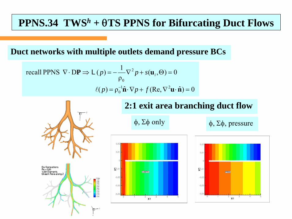
Duct networks with multiple outlets demand pressure BCs

φ, Σφ only

2:1 exit area branching duct flow

0)ˆ(Re,ˆρ)(

0),(ρ1)(DPPNSrecall

210

2

0

=⋅∇+∇⋅=

=Θ+∇−=⇒⋅∇

− nun

uP

fpp

spp iL

φ, Σφ, pressure

PPNS.34 TWSh + θTS PPNS for Bifurcating Duct Flows

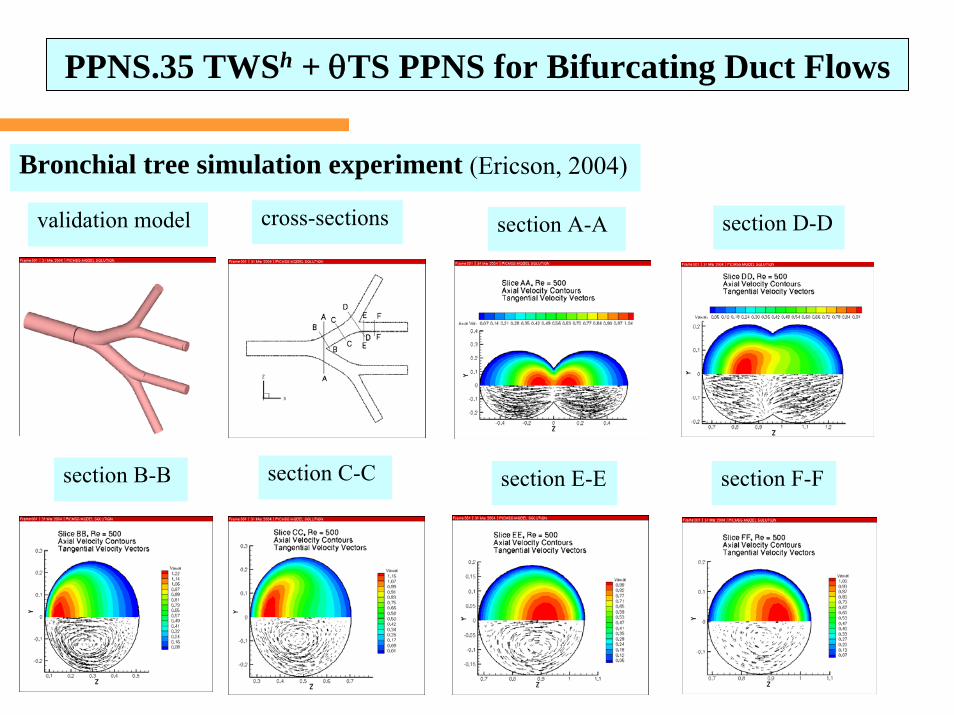
Bronchial tree simulation experiment (Ericson, 2004)

validation model cross-sections

section B-B

section A-A section D-D

section C-C section E-E section F-F

PPNS.35 TWSh + θTS PPNS for Bifurcating Duct Flows

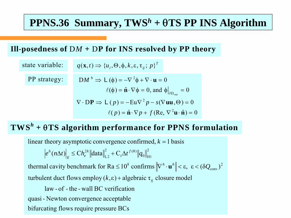
Ill-posedness of DM + DP for INS resolved by PP theory

TWSh + θTS algorithm performance for PPNS formulation

Tiji pkutq };τ,,,,,{),( εφΘ⇒xstate variable:

PP strategy:

0)ˆ(Re,ˆ)(0),(Eu)(D

0and,0ˆ)(0)(D

2

2

2

out

=⋅∇+∇⋅=

=Θ∇−∇−=⇒⋅∇

=φ=φ∇⋅=φ

=⋅∇+φ−∇=φ⇒

Ω∂

nunuuP

nu

fppspp

M h

L

L

BCspressurerequireflowsgbifurcatinacceptableeconvergencNewton-quasi

onverificatiBCwall-the-of-law

modelclosureτalgebraic),(employ flowsductturbulent

)(δεε,confirms10Raforbenchmarkcavitythermal

CdataC)(

basis1,confirmedeconvergencasymptotictheorylinear

2conv

8

2

1H0)(2

2L2

ij

hh

ft

keE

h

k

Q

qthtne

k

+ε

<<⋅∇≤

Δ+≤Δ

=θ

u

PPNS.36 Summary, TWSh + θTS PP INS Algorithm

PPNS.1 Pressure Projection Algorithms for...

Documents

Transcript of PPNS.1 Pressure Projection Algorithms for...