Reiter’s Projection and Perturbation

Algorithm Applied to a Search-and-Matching

Model

Julien Pascal

05/03/2018

Sciences Po and LIEPP

1

Road map

Outline

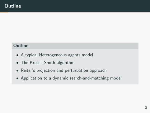
Outline

• A typical Heterogeneous agents model

• The Krusell-Smith algorithm

• Reiter’s projection and perturbation approach

• Application to a dynamic search-and-matching model

2

A typical heterogeneous agents

model

Model

Households with idiosyncratic labor income shocks:

• continuum of utility-maximizing households indexed by

j ∈ [0, 1]:

maxcjt∞t=0

(E

+∞∑t=0

βtc1−σjt − 1

1− σ)

such that:

cjt + kjt+1 − (1− δ)kjt = yjt

• inelastic labor supply l , shock εjt independent across

households, follows 2-state Markov process within households:

εjt ∈ ε0 = 0, ε1 = 1

• labor earnings:

yjt =

wt l if εjt = 1 (employed)

0 if εjt = 0 (unemployed)3

Model

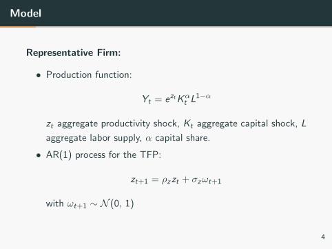
Representative Firm:

• Production function:

Yt = eztKαt L

1−α

zt aggregate productivity shock, Kt aggregate capital shock, L

aggregate labor supply, α capital share.

• AR(1) process for the TFP:

zt+1 = ρzzt + σzωt+1

with ωt+1 ∼ N (0, 1)

4

Model

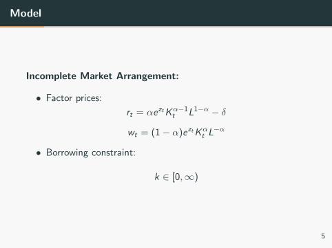
Incomplete Market Arrangement:

• Factor prices:

rt = αeztKα−1t L1−α − δ

wt = (1− α)eztKαt L−α

• Borrowing constraint:

k ∈ [0,∞)

5

Model

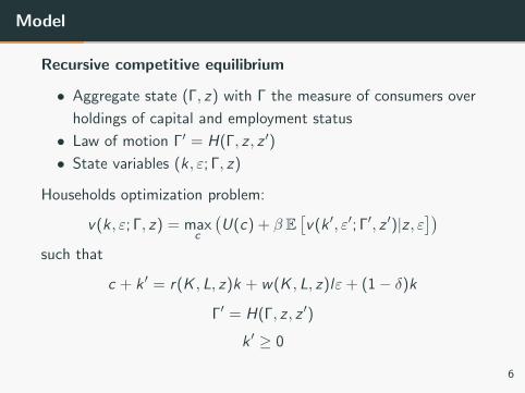
Recursive competitive equilibrium

• Aggregate state (Γ, z) with Γ the measure of consumers over

holdings of capital and employment status

• Law of motion Γ′ = H(Γ, z , z ′)

• State variables (k , ε; Γ, z)

Households optimization problem:

v(k, ε; Γ, z) = maxc

(U(c) + β E

[v(k ′, ε′; Γ′, z ′)|z , ε

])such that

c + k ′ = r(K , L, z)k + w(K , L, z)lε+ (1− δ)k

Γ′ = H(Γ, z , z ′)

k ′ ≥ 0

6

Model

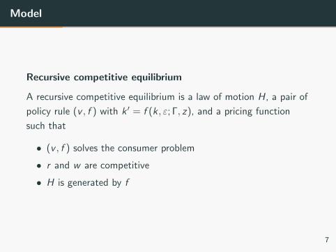
Recursive competitive equilibrium

A recursive competitive equilibrium is a law of motion H, a pair of

policy rule (v , f ) with k ′ = f (k , ε; Γ, z), and a pricing function

such that

• (v , f ) solves the consumer problem

• r and w are competitive

• H is generated by f

7

Krusell-Smith Algorithm

Krusell-Smith Algorithm

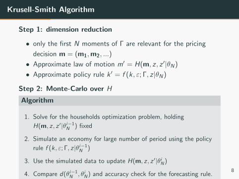
Step 1: dimension reduction

• only the first N moments of Γ are relevant for the pricing

decision m = (m1,m2, ...)

• Approximate law of motion m′ = H(m, z , z ′|θN)

• Approximate policy rule k ′ = f (k , ε; Γ, z |θN)

Step 2: Monte-Carlo over H

Algorithm

1. Solve for the households optimization problem, holding

H(m, z , z ′|θi−1N ) fixed

2. Simulate an economy for large number of period using the policy

rule f (k, ε; Γ, z |θi−1N )

3. Use the simulated data to update H(m, z , z ′|θiN)

4. Compare d(θi−1N , θiN) and accuracy check for the forecasting rule.

8

Example Krusell-Smith Algorithm

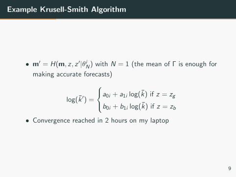
• m′ = H(m, z , z ′|θiN) with N = 1 (the mean of Γ is enough for

making accurate forecasts)

log(k ′) =

a0i + a1i log(k) if z = zg

b0i + b1i log(k) if z = zb

• Convergence reached in 2 hours on my laptop

9

Reiter’s projection and perturbation

method

General Idea

• Circumvent the need for finding H by Monte-Carlo

• Projection: finite representation of the infinite dimensional

problem by using an histogram to approximate Γ

• Perturbation: solve for a steady-state of the finite model and

use perturbation method around the steady-state

10

Model

Reiter (2009) is Krusell and Smith (1998) with 2 modifications:

• stochastic tax rate following an AR(1) process:

τt+1 − τ∗ = ρt(τt − τ∗) + ετ,t+1

The government taxes end-of-the period capital kt−1. Lump

sum redistribution to households at the beginning of period t.

Balanced budget at every period.

• Continuous distribution of idiosyncratic shocks ξit , i.i.d, with

pdf fξ(.) and cdf Fξ(.). Normalization:

Et [ξit ] = Et−1[ξit ] = 1

11

Equilibrium

State variables

Ωt = (Zt , τt ,Ψk,t−1(.))

with

• Zt the aggregate productivity variable in period t

• τt the tax rate in period t

• Ψk,t−1(.) the cross-sectional distribution of capital holdings

inherited from period t − 1

12

Equilibrium

Definition An equilibrium consists in:

• a consumption function C (χ,Ωt) with χ after-transfer

disposable income in period t

χit = (1 + rt)kt−1 + wtξit + Tt

• a stochastic process of cross-sectional distribution Ψk,t(.)

• a process of lump sum transfers Tt

such that:

• C (χ,Ωt) satisfies the Euler equation

• Ψk,t(.) is consistent with the dynamic equation implied by the

Euler equation

• Transfers satisfy the balanced budget condition

13

(Reiter, 2009) 3-step approach

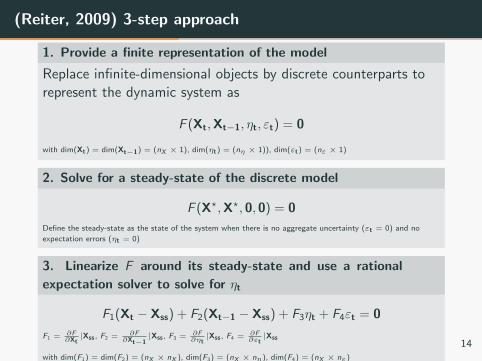
1. Provide a finite representation of the model

Replace infinite-dimensional objects by discrete counterparts torepresent the dynamic system as

F (Xt,Xt−1, ηt, εt) = 0

with dim(Xt) = dim(Xt−1) = (nX × 1), dim(ηt) = (nη × 1)), dim(εt) = (nε × 1)

2. Solve for a steady-state of the discrete model

F (X?,X?, 0, 0) = 0

Define the steady-state as the state of the system when there is no aggregate uncertainty (εt = 0) and no

expectation errors (ηt = 0)

3. Linearize F around its steady-state and use a rational

expectation solver to solve for ηt

F1(Xt − Xss) + F2(Xt−1 − Xss) + F3ηt + F4εt = 0

F1 = ∂F∂Xt|Xss, F2 = ∂F

∂Xt−1|Xss, F3 = ∂F

∂ηt|Xss, F4 = ∂F

∂εt|Xss

with dim(F1) = dim(F2) = (nX × nX ), dim(F3) = (nX × nη), dim(F4) = (nX × nε)

14

Discretezing the model

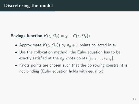
Savings function K (χ,Ωt) = χ− C (χ,Ωt))

• Approximate K (χ,Ωt)) by np + 1 points collected in st.

• Use the collocation method: the Euler equation has to be

exactly satisfied at the np knots points [χt,1, ..., χt,np ].

• Knots points are chosen such that the borrowing constraint is

not binding (Euler equation holds with equality)

15

Discretezing the model

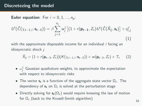
Euler equation: For i = 0, 1, ..., np:

U ′(C (χt−1,i ; st−1)) = β

nζ∑j=1

w ζj

[(1 + r(pt−1,Zt)U

′(C (Xij , st)]

+ ηci ,j

(1)with the approximate disposable income for an individual i facing an

idiosyncratic shock j

Xij = (1 + r(pt−1,Zt))(K (χt−1,i ; st−1)) + w(pt−1,Zt) + Tt (2)

• ωζj Gaussian quadrature weights, to approximate the expectation

with respect to idiosyncratic risks

• The vector st is a function of the aggregate state vector Ωt . The

dependency of st on Ωt is solved at the perturbation stage

• Directly solving for st(Ωt) would require knowing the law of motion

for Ωt (back to the Krusell-Smith algorithm)16

Discretezing the model

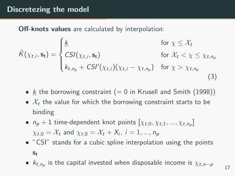
Off-knots values are calculated by interpolation:

K (χt,i , st) =

k for χ ≤ Xt

CSI (χt,i , st) for Xt < χ ≤ χt,np

kt,np + CSI ′(χt,i )(χt,i − χt,np) for χ > χt,np

(3)

• k the borrowing constraint (= 0 in Krusell and Smith (1998))

• Xt the value for which the borrowing constraint starts to be

binding

• np + 1 time-dependent knot points [χt,0, χt,1, ..., χt,np ]

χt,0 = Xt and χt,0 = Xt + Xi , i = 1, ..., np

• ”CSI” stands for a cubic spline interpolation using the points

st

• kt,np is the capital invested when disposable income is χt,n−p17

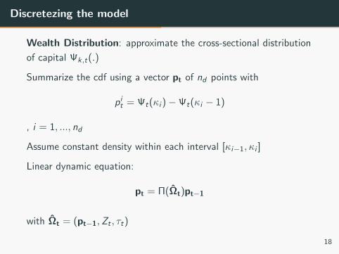
Discretezing the model

Wealth Distribution: approximate the cross-sectional distribution

of capital Ψk,t(.)

Summarize the cdf using a vector pt of nd points with

pit = Ψt(κi )−Ψt(κi − 1)

, i = 1, ..., nd

Assume constant density within each interval [κi−1, κi ]

Linear dynamic equation:

pt = Π(Ωt)pt−1

with Ωt = (pt−1,Zt , τt)

18

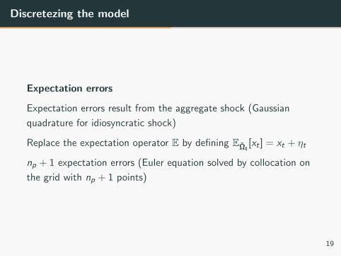
Discretezing the model

Expectation errors

Expectation errors result from the aggregate shock (Gaussian

quadrature for idiosyncratic shock)

Replace the expectation operator E by defining EΩt[xt ] = xt + ηt

np + 1 expectation errors (Euler equation solved by collocation on

the grid with np + 1 points)

19

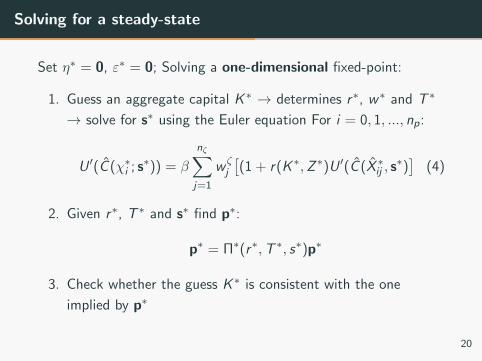
Solving for a steady-state

Set η∗ = 0, ε∗ = 0; Solving a one-dimensional fixed-point:

1. Guess an aggregate capital K ∗ → determines r∗, w∗ and T ∗

→ solve for s∗ using the Euler equation For i = 0, 1, ..., np:

U ′(C (χ∗i ; s∗)) = β

nζ∑j=1

w ζj

[(1 + r(K ∗,Z ∗)U ′(C (X ∗ij , s

∗)]

(4)

2. Given r∗, T ∗ and s∗ find p∗:

p∗ = Π∗(r∗,T ∗, s∗)p∗

3. Check whether the guess K ∗ is consistent with the one

implied by p∗

20

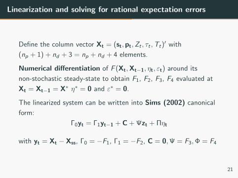
Linearization and solving for rational expectation errors

Define the column vector Xt = (st,pt,Zt , τt ,Tt)′ with

(np + 1) + nd + 3 = np + nd + 4 elements.

Numerical differentiation of F (Xt,Xt−1, ηt, εt) around its

non-stochastic steady-state to obtain F1, F2, F3, F4 evaluated at

Xt = Xt−1 = X∗ η∗ = 0 and ε∗ = 0.

The linearized system can be written into Sims (2002) canonical

form:

Γ0yt = Γ1yt−1 + C + Ψzt + Πηt

with yt = Xt − Xss, Γ0 = −F1, Γ1 = −F2, C = 0,Ψ = F3,Φ = F4

21

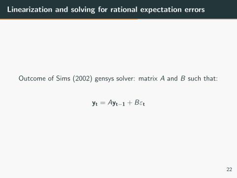
Linearization and solving for rational expectation errors

Outcome of Sims (2002) gensys solver: matrix A and B such that:

yt = Ayt−1 + Bεt

22

Projection and Perturbation in a

Search-and-Matching Model

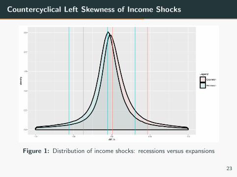
Countercyclical Left Skewness of Income Shocks

Figure 1: Distribution of income shocks: recessions versus expansions

23

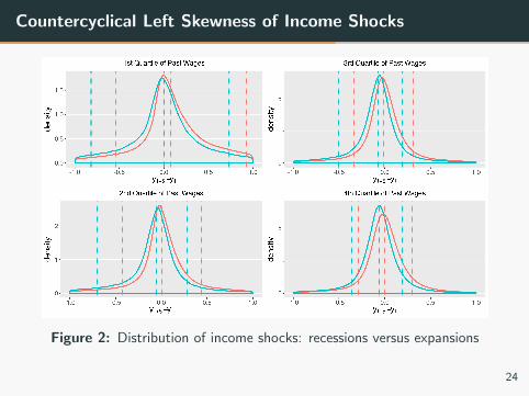
Countercyclical Left Skewness of Income Shocks

Figure 2: Distribution of income shocks: recessions versus expansions

24

Our Contribution

Main Question

What are the impacts of payroll taxation on labor income risks

along the business cycle?

Contribution

• Build a dynamic history-dependent︸ ︷︷ ︸Technical contribution

model with non-linear

taxes on wages, frictional unemployment and heterogeneous

workers

• Counter-factual: ”flat-tax”

25

Literature

Empirical Literature

• Guvenen, Ozkan, and Song (2014) Busch, Domeij, Guvenen, and Madera (2015)

Costs of Business Cycle

• Lucas Jr (2003) Gali, Gertler, and Lopez-Salido (2007)

• Clark and Oswald (1994) Wolfers (2003) Clark, Diener, Georgellis, and Lucas (2008) Aghion, Akcigit,

Deaton, and Roulet (2015)

Optimal Labor Taxation

• Mirrlees (1971), Saez (2001), Kleven, Kreiner, and Saez (2009)

Taxation in Search-and-Matching Models

• Cheron, Hairault, and Langot (2008) Carbonnier et al. (2014), Breda, Haywood, and Haomin (2016)

26

Model

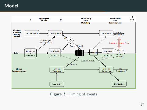
Model

Figure 3: Timing of events

27

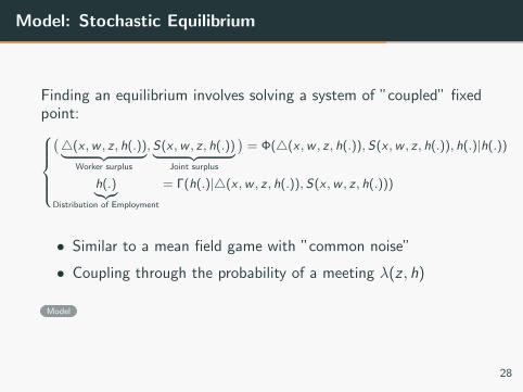
Model: Stochastic Equilibrium

Finding an equilibrium involves solving a system of ”coupled” fixedpoint:(4(x ,w , z , h(.))︸ ︷︷ ︸

Worker surplus

, S(x ,w , z , h(.))︸ ︷︷ ︸Joint surplus

)= Φ(4(x ,w , z , h(.)),S(x ,w , z , h(.)), h(.)|h(.))

h(.)︸︷︷︸Distribution of Employment

= Γ(h(.)|4(x ,w , z , h(.)),S(x ,w , z , h(.)))

• Similar to a mean field game with ”common noise”

• Coupling through the probability of a meeting λ(z , h)

Model

28

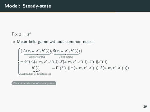
Model: Steady-state

Fix z = z∗

≈ Mean field game without common noise:

(4(x ,w , z∗, h∗(.))︸ ︷︷ ︸

Worker surplus

, S(x ,w , z∗, h∗(.))︸ ︷︷ ︸Joint surplus

)= Φ∗(4(x ,w , z∗, h∗(.)),S(x ,w , z∗, h∗(.)), h∗(.)|h∗(.))

h∗(.)︸ ︷︷ ︸Distribution of Employment

= Γ∗(h∗(.)|4(x ,w , z∗, h∗(.)), S(x ,w , z∗, h∗(.)))

Discussion existence of a steady-state

29

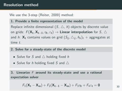
Resolution method

We use the 3-step (Reiter, 2009) method:

1. Provide a finite representation of the model

Replace infinite dimensional (S , 4, h) objects by discrete value

on grids: F (Xt,Xt−1, ηt, εt) → Linear interpolation for S , 4and h: Xt contains values on grid (Sij ,4ij , hk)t + aggregates at

time t.

2. Solve for a steady-state of the discrete model

• Solve for S and 4 holding fixed h

• Solve for h holding fixed S and 4

3. Linearize F around its steady-state and use a rational

expectation solver

F1(Xt − Xss) + F2(Xt−1 − Xss) + F3ηt + F4εt = 0 30

Flat tax counter-factual

Flat tax counter-factual: Idea

Figure 4: The Hall–Rabushka flat tax (1985)31

Flat tax counter-factual: experiment

1. Estimate the model using Italian data

2. Find a flat tax such that the government revenue = constant

3. Simulate ”step function” and ”flat” tax economies and

compare

32

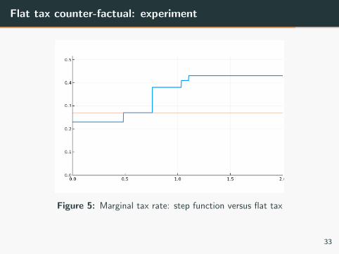
Flat tax counter-factual: experiment

Figure 5: Marginal tax rate: step function versus flat tax

33

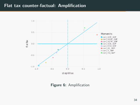
Flat tax counter-factual: Amplification

Figure 6: Amplification

34

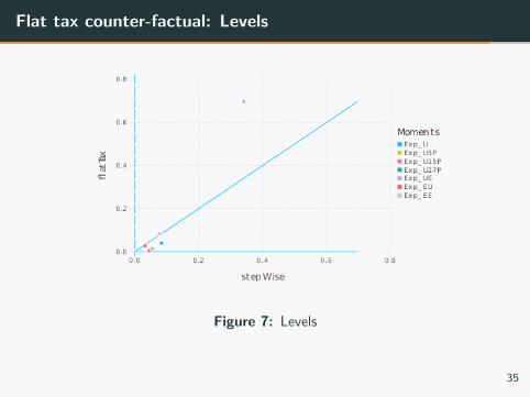
Flat tax counter-factual: Levels

Figure 7: Levels

35

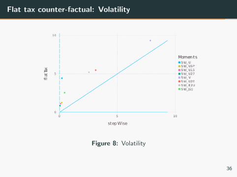
Flat tax counter-factual: Volatility

Figure 8: Volatility

36

Conclusion

Conclusion

Main Question

What are the impacts of payroll taxation on labor income risks

along the business cycle?

Preliminary Answers

• payroll taxation as a tool to mitigate labor income shocks

• trade-off level - volatility

Work In Progress

• Estimation

• Counter-factuals

• Firm heterogeneity

37

Questions?

37

38

References I

References

Aghion, P., Akcigit, U., Deaton, A., & Roulet, A. (2015). Creative

destruction and subjective wellbeing (Tech. Rep.). National

Bureau of Economic Research.

Breda, T., Haywood, L., & Haomin, W. (2016). Labor market

responses to taxes and minimum wage policies. Working

Paper.

Busch, C., Domeij, D., Guvenen, F., & Madera, R. (2015).

Asymmetric business cycle risk and government insurance

(Tech. Rep.). Working Paper.

References II

Carbonnier, C., et al. (2014). Payroll taxation and the structure of

qualifications and wages in a segmented frictional labor

market with intrafirm bargaining (Tech. Rep.). THEMA

(THeorie Economique, Modelisation et Applications),

Universite de Cergy-Pontoise.

Cheron, A., Hairault, J.-O., & Langot, F. (2008). A quantitative

evaluation of payroll tax subsidies for low-wage workers: An

equilibrium search approach. Journal of Public Economics,

92(3), 817–843.

Clark, A. E., Diener, E., Georgellis, Y., & Lucas, R. E. (2008).

Lags and leads in life satisfaction: A test of the baseline

hypothesis. The Economic Journal, 118(529).

References III

Clark, A. E., & Oswald, A. J. (1994). Unhappiness and

unemployment. The Economic Journal, 104(424), 648–659.

Gali, J., Gertler, M., & Lopez-Salido, J. D. (2007). Markups, gaps,

and the welfare costs of business fluctuations. The review of

economics and statistics, 89(1), 44–59.

Guvenen, F., Ozkan, S., & Song, J. (2014). The nature of

countercyclical income risk. Journal of Political Economy,

122(3), 621–660.

Kleven, H. J., Kreiner, C. T., & Saez, E. (2009). The optimal

income taxation of couples. Econometrica, 77(2), 537–560.

Krusell, P., & Smith, A. A., Jr. (1998). Income and wealth

heterogeneity in the macroeconomy. Journal of political

Economy, 106(5), 867–896.

References IV

Lucas Jr, R. E. (2003). Macroeconomic priorities. American

economic review, 93(1), 1–14.

Mirrlees, J. A. (1971). An exploration in the theory of optimum

income taxation. The review of economic studies, 38(2),

175–208.

Reiter, M. (2009). Solving heterogeneous-agent models by

projection and perturbation. Journal of Economic Dynamics

and Control, 33(3), 649–665.

Robin, J.-M. (2011). On the dynamics of unemployment and wage

distributions. Econometrica, 79(5), 1327–1355.

Saez, E. (2001). Using elasticities to derive optimal income tax

rates. The review of economic studies, 68(1), 205–229.

References V

Sims, C. A. (2002). Solving linear rational expectations models.

Computational economics, 20(1), 1–20.

Wolfers, J. (2003). Is business cycle volatility costly? evidence

from surveys of subjective well-being. International finance,

6(1), 1–26.

Model

Workers, Firms and Production

• continuum of infinitely-lived workers differing in their individual

productivity, indexed by x .

• distribution of ability x is exogenous and denoted by `(x).

• firms are identical and can freely enter the market, incurring an

exogenous cost c(v) when posting v vacancies.

• when matched firms and workers produce a per period output

p(x , zt).

Shocks:

• aggregate productivity z follows and AR(1) process

Back

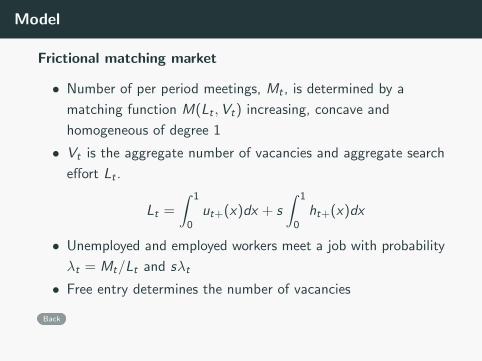
Model

Frictional matching market

• Number of per period meetings, Mt , is determined by a

matching function M(Lt ,Vt) increasing, concave and

homogeneous of degree 1

• Vt is the aggregate number of vacancies and aggregate search

effort Lt .

Lt =

∫ 1

0ut+(x)dx + s

∫ 1

0ht+(x)dx

• Unemployed and employed workers meet a job with probability

λt = Mt/Lt and sλt

• Free entry determines the number of vacancies

Back

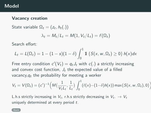
Model

Vacancy creation

State variable Ωt = (zt , ht(.))

λt = Mt/Lt = M(1,Vt/Lt) = f (Ωt)

Search effort:

Lt = L(Ωt) = 1− (1− s)(1− δ)

∫ 1

011 S(x ,w ,Ωt) ≥ 0 h(x)dx

Free entry condition c ′(Vt) = qtJt with c(.) a strictly increasingand convex cost function, Jt the expected value of a filledvacancy,qt the probability for meeting a worker

Vt = V (Ωt) = (c ′)−1(M( 1

VtLt,

1

Lt

) ∫ 1

0

(`(x)−(1−δ)h(x)) maxS(x ,w ,Ωt), 0)

L.h.s strictly increasing in Vt , r.h.s strictly decreasing in Vt . → Vt

uniquely determined at every period t.

Back

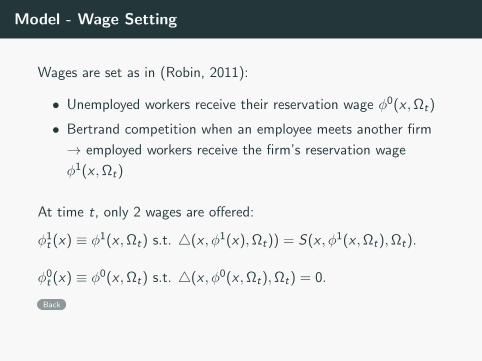
Model - Wage Setting

Wages are set as in (Robin, 2011):

• Unemployed workers receive their reservation wage φ0(x ,Ωt)

• Bertrand competition when an employee meets another firm

→ employed workers receive the firm’s reservation wage

φ1(x ,Ωt)

At time t, only 2 wages are offered:

φ1t (x) ≡ φ1(x ,Ωt) s.t. 4(x , φ1(x),Ωt)) = S(x , φ1(x ,Ωt),Ωt).

φ0t (x) ≡ φ0(x ,Ωt) s.t. 4(x , φ0(x ,Ωt),Ωt) = 0.

Back

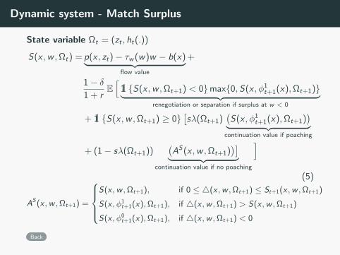
Dynamic system - Match Surplus

State variable Ωt = (zt , ht(.))

S(x ,w ,Ωt) = p(x , zt)− τw (w)w − b(x)︸ ︷︷ ︸flow value

+

1− δ1 + r

E[

11 S(x ,w ,Ωt+1) < 0max0,S(x , φ1t+1(x),Ωt+1)︸ ︷︷ ︸

renegotiation or separation if surplus at w < 0

+ 11 S(x ,w ,Ωt+1) ≥ 0[sλ(Ωt+1)

(S(x , φ1

t+1(x),Ωt+1))︸ ︷︷ ︸

continuation value if poaching

+ (1− sλ(Ωt+1))(AS(x ,w ,Ωt+1)

)]︸ ︷︷ ︸continuation value if no poaching

](5)

AS(x ,w ,Ωt+1) =

S(x ,w ,Ωt+1), if 0 ≤ 4(x ,w ,Ωt+1) ≤ St+1(x ,w ,Ωt+1)

S(x , φ1t+1(x),Ωt+1), if 4(x ,w ,Ωt+1) > S(x ,w ,Ωt+1)

S(x , φ0t+1(x),Ωt+1), if 4(x ,w ,Ωt+1) < 0

Back

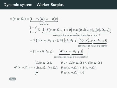
Dynamic system - Worker Surplus

4(x ,w ,Ωt) = [1− τw (w)]w − b(x)︸ ︷︷ ︸flow value

+

1− δ1 + r

E[

11 S(x ,w ,Ωt+1) < 0max0,S(x , φ1t+1(x),Ωt+1)︸ ︷︷ ︸

renegotiation or separation if surplus at w < 0

+ 11 S(x ,w ,Ωt+1) ≥ 0[sλ(Ωt+1)

(S(x , φ1

t+1(x),Ωt+1))︸ ︷︷ ︸

continuation value if poached

+ (1− sλ(Ωt+1))(A4(x ,w ,Ωt+1)

)]︸ ︷︷ ︸continuation value if not poached

]

Aw (x ,w ,Ωt) =

4(x ,w ,Ωt), if 0 ≤ 4(x ,w ,Ωt) ≤ S(x ,w ,Ωt)

S(x , φ1t+1(x),Ωt), if 4(x ,w ,Ωt) > S(x ,w ,Ωt)

0, if 4(x ,w ,Ωt) < 0

Back

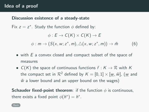
Idea of a proof

Discussion existence of a steady-state

Fix z = z∗. Study the function φ defined by:

φ : E → C (K )× C (K )→ E

φ : m→ (S(x ,w ; z∗,m),4(x ,w ; z∗,m))→ m (6)

• with E a convex closed and compact subset of the space of

measures

• C (K ) the space of continuous functions f : K → R with K

the compact set in R2 defined by K = [0, 1]× [w , w ], (w and

w a lower bound and an upper bound on the wages)

Schauder fixed-point theorem: if the function φ is continuous,

there exists a fixed point φ(h∗) = h∗.

Back

Idea of a proof

Discussion existence of a steady-state

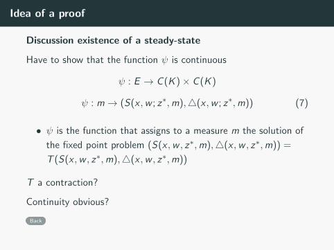
Have to show that the function ψ is continuous

ψ : E → C (K )× C (K )

ψ : m→ (S(x ,w ; z∗,m),4(x ,w ; z∗,m)) (7)

• ψ is the function that assigns to a measure m the solution of

the fixed point problem (S(x ,w , z∗,m),4(x ,w , z∗,m)) =

T (S(x ,w , z∗,m),4(x ,w , z∗,m))

T a contraction?

Continuity obvious?

Back

Idea of a proof

Discussion existence of a steady-state

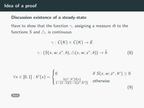
Have to show that the function γ, assigning a measure m to the

functions S and 4, is continuous

γ : C (K )× C (K )→ E

γ : (S(x ,w ; z∗, h),4(x ,w ; z∗, h))→ h (8)

∀x ∈ [0, 1] : h∗(x) =

0 if S(x ,w ; z∗, h∗) ≥ 0λ(z∗,h∗)l(x)

1−(1−δ)(1−λ(z∗,h∗)) otherwise

(9)

Back