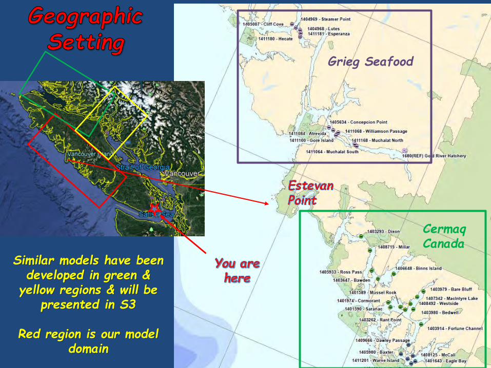
Similar models have been developed in green &

yellow regions & will be presented in S3

Red region is our model domain

CermaqCanada

Grieg Seafood

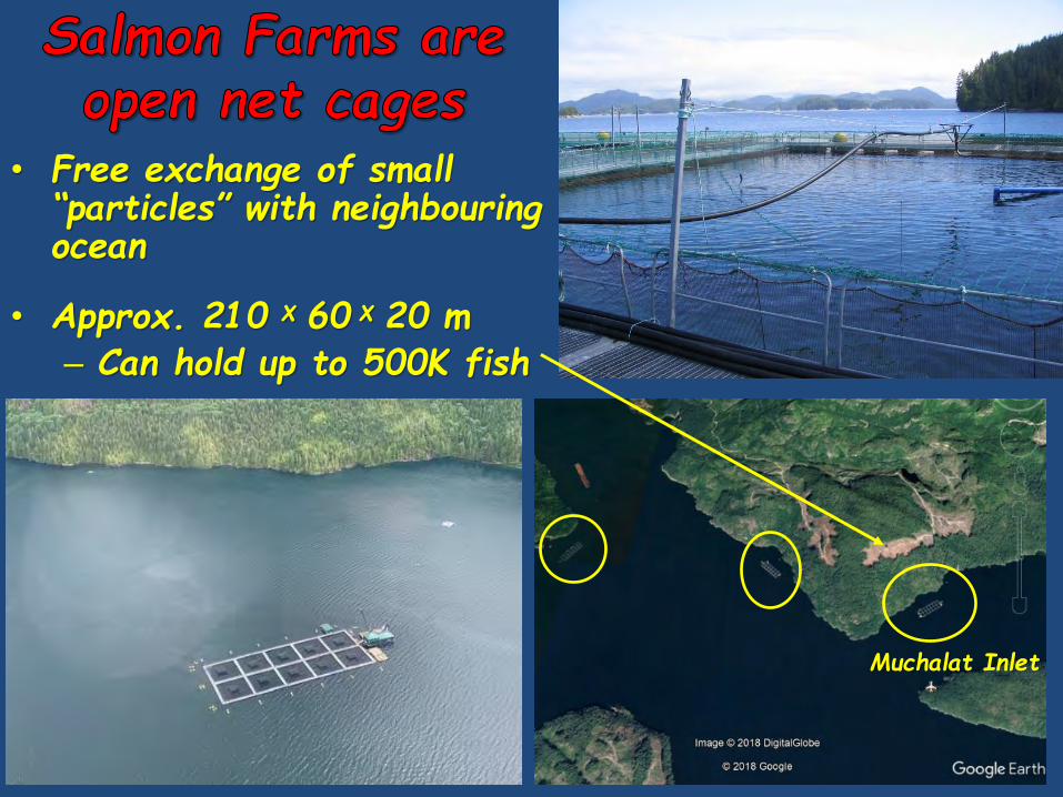
• Free exchange of small “particles” with neighbouring ocean

• Approx. 210 χ 60 χ 20 m– Can hold up to 500K fish

Muchalat Inlet

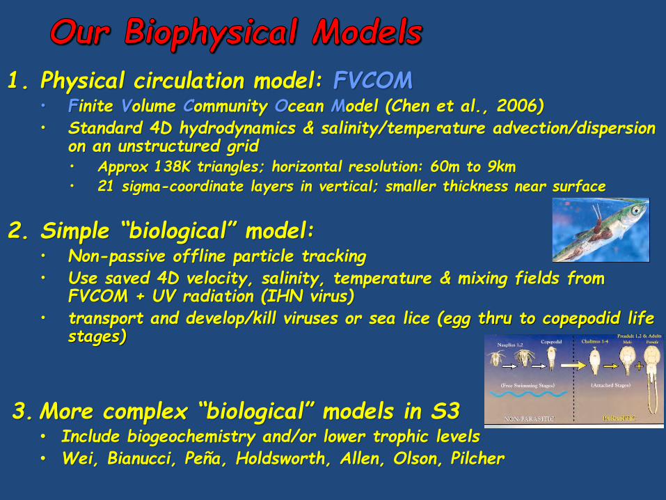
1. Physical circulation model: FVCOM• Finite Volume Community Ocean Model (Chen et al., 2006)• Standard 4D hydrodynamics & salinity/temperature advection/dispersion

on an unstructured grid • Approx 138K triangles; horizontal resolution: 60m to 9km• 21 sigma-coordinate layers in vertical; smaller thickness near surface

2. Simple “biological” model:• Non-passive offline particle tracking• Use saved 4D velocity, salinity, temperature & mixing fields from

FVCOM + UV radiation (IHN virus)• transport and develop/kill viruses or sea lice (egg thru to copepodid life

stages)

3.More complex “biological” models in S3• Include biogeochemistry and/or lower trophic levels • Wei, Bianucci, Peña, Holdsworth, Allen, Olson, Pilcher

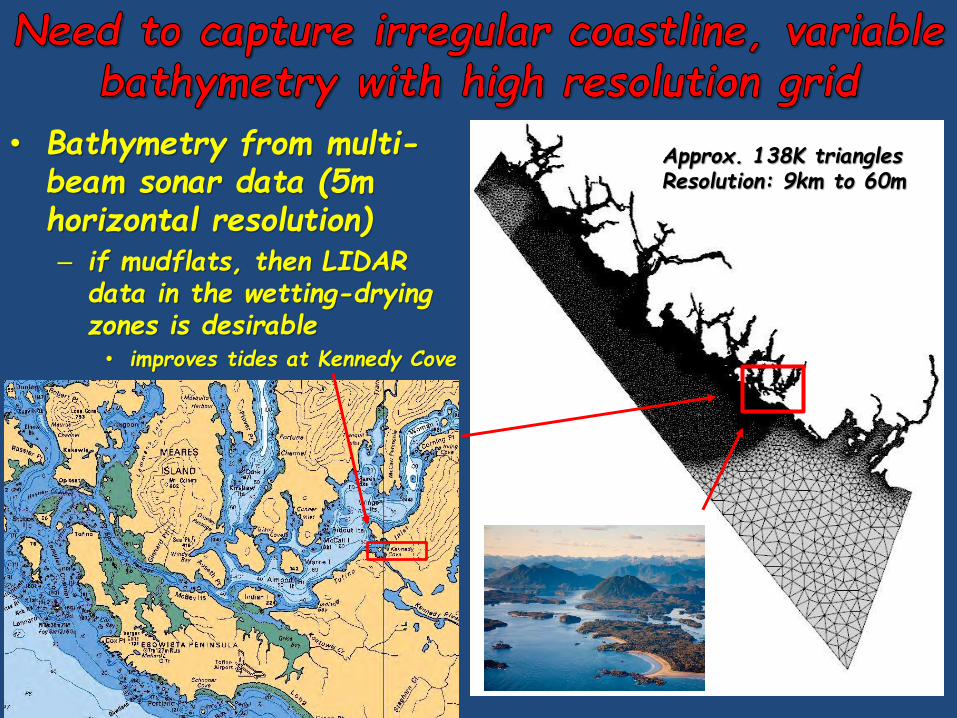
• Bathymetry from multi-beam sonar data (5m horizontal resolution) – if mudflats, then LIDAR

data in the wetting-drying zones is desirable• improves tides at Kennedy Cove

Approx. 138K trianglesResolution: 9km to 60m

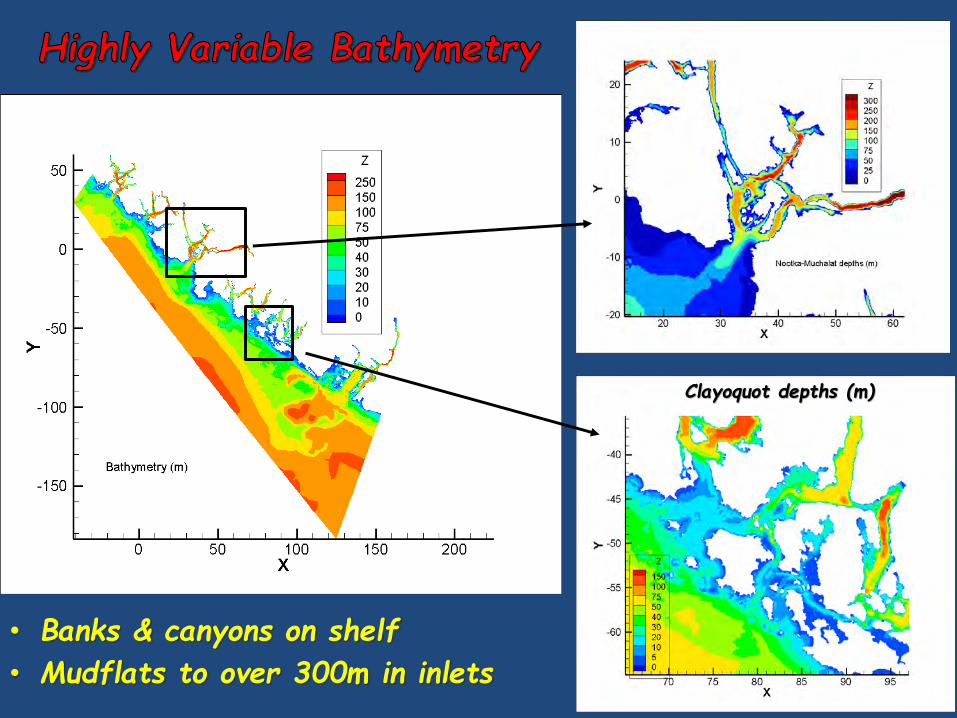
• Banks & canyons on shelf

• Mudflats to over 300m in inlets

Clayoquot depths (m)

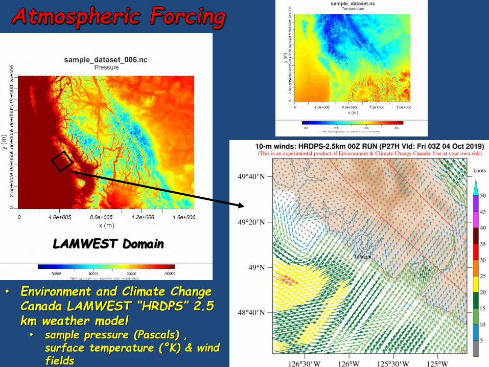
• Environment and Climate Change Canada LAMWEST “HRDPS” 2.5 km weather model• sample pressure (Pascals) ,

surface temperature (°K) & wind fields

LAMWEST Domain

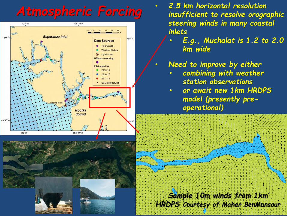
Atmospheric Forcing • 2.5 km horizontal resolution

insufficient to resolve orographic steering winds in many coastal inlets• E.g., Muchalat is 1.2 to 2.0

km wide

• Need to improve by either • combining with weather

station observations • or await new 1km HRDPS

model (presently pre-operational)

Sample 10m winds from 1km HRDPS Courtesy of Maher BenMansour

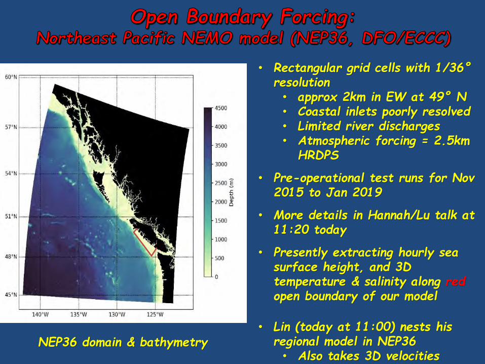
• Rectangular grid cells with 1/36°resolution • approx 2km in EW at 49° N• Coastal inlets poorly resolved• Limited river discharges• Atmospheric forcing = 2.5km

HRDPS

• Pre-operational test runs for Nov 2015 to Jan 2019

• More details in Hannah/Lu talk at 11:20 today

• Presently extracting hourly sea surface height, and 3D temperature & salinity along red open boundary of our model

• Lin (today at 11:00) nests his regional model in NEP36• Also takes 3D velocities

NEP36 domain & bathymetry

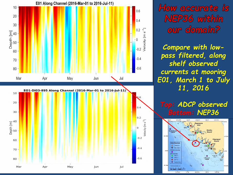
Compare with low-pass filtered, along

shelf observed currents at mooring

E01, March 1 to July 11, 2016

Top: ADCP observed Bottom: NEP36

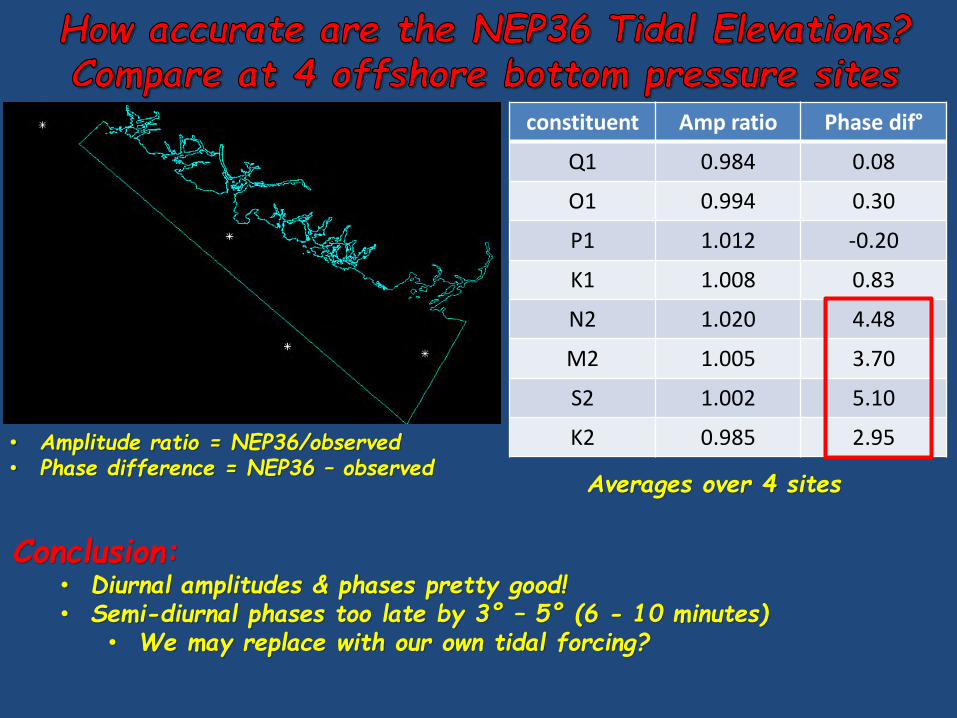
constituent Amp ratio Phase dif°

Q1 0.984 0.08

O1 0.994 0.30

P1 1.012 -0.20

K1 1.008 0.83

N2 1.020 4.48

M2 1.005 3.70

S2 1.002 5.10

K2 0.985 2.95• Amplitude ratio = NEP36/observed• Phase difference = NEP36 – observed

Conclusion:• Diurnal amplitudes & phases pretty good!• Semi-diurnal phases too late by 3° – 5° (6 - 10 minutes)

• We may replace with our own tidal forcing?

Averages over 4 sites

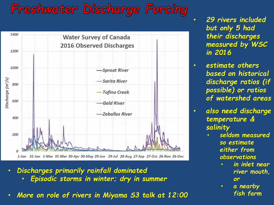
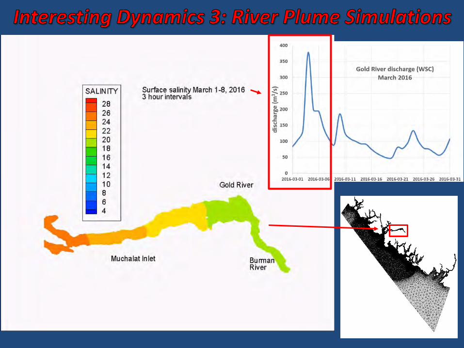
• Discharges primarily rainfall dominated• Episodic storms in winter; dry in summer

• More on role of rivers in Miyama S3 talk at 12:00

• 29 rivers included but only 5 had their discharges measured by WSC in 2016

• estimate others based on historical discharge ratios (if possible) or ratios of watershed areas

• also need discharge temperature & salinity • seldom measured

so estimate either from observations • in inlet near

river mouth, or

• a nearby fish farm

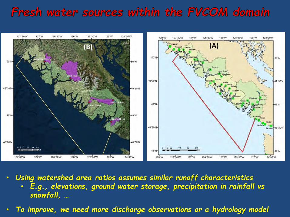
• Using watershed area ratios assumes similar runoff characteristics• E.g., elevations, ground water storage, precipitation in rainfall vs

snowfall, …

• To improve, we need more discharge observations or a hydrology model

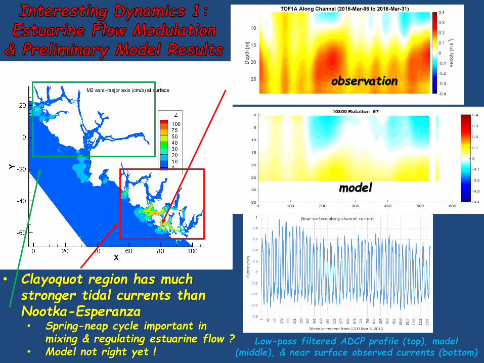
• Clayoquot region has much stronger tidal currents than Nootka-Esperanza• Spring-neap cycle important in

mixing & regulating estuarine flow ?• Model not right yet !

Low-pass filtered ADCP profile (top), model (middle), & near surface observed currents (bottom)

observation

model

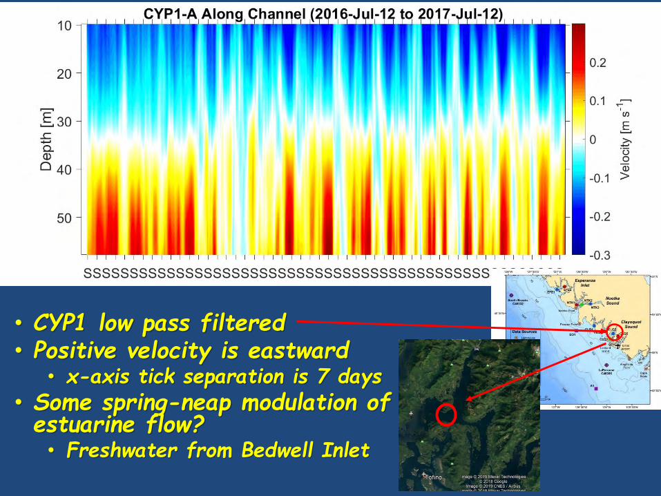
• CYP1 low pass filtered• Positive velocity is eastward

• x-axis tick separation is 7 days• Some spring-neap modulation of estuarine flow?• Freshwater from Bedwell Inlet

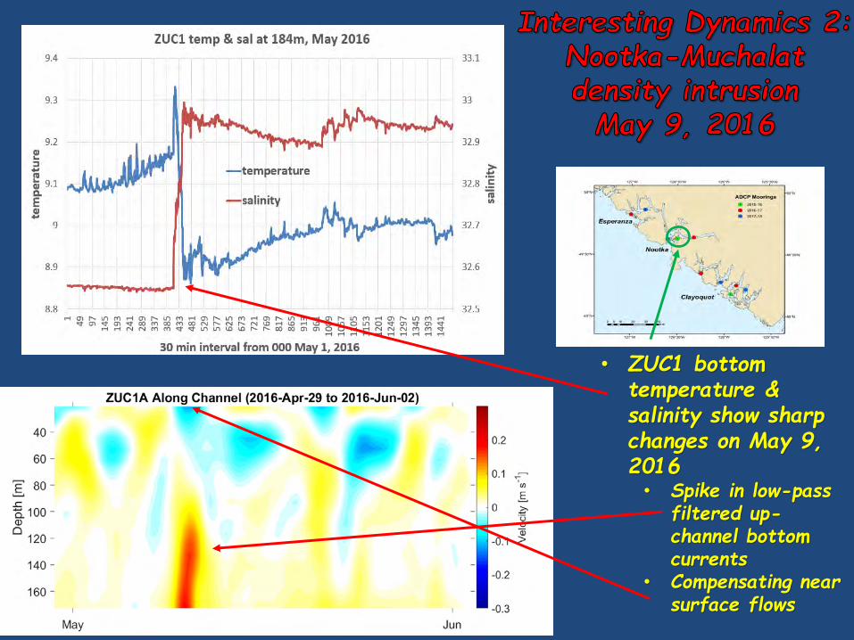
• ZUC1 bottom temperature & salinity show sharp changes on May 9, 2016• Spike in low-pass

filtered up-channel bottom currents

• Compensating near surface flows

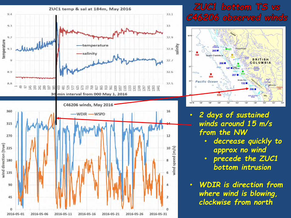
• 2 days of sustained winds around 15 m/s from the NW • decrease quickly to

approx no wind • precede the ZUC1

bottom intrusion

• WDIR is direction from where wind is blowing, clockwise from north

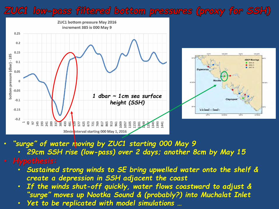
• “surge” of water moving by ZUC1 starting 000 May 9 • 29cm SSH rise (low-pass) over 2 days; another 8cm by May 15

• Hypothesis:• Sustained strong winds to SE bring upwelled water onto the shelf &

create a depression in SSH adjacent the coast• If the winds shut-off quickly, water flows coastward to adjust &

“surge” moves up Nootka Sound & (probably?) into Muchalat Inlet• Yet to be replicated with model simulations …

1 dbar ~ 1cm sea surface height (SSH)

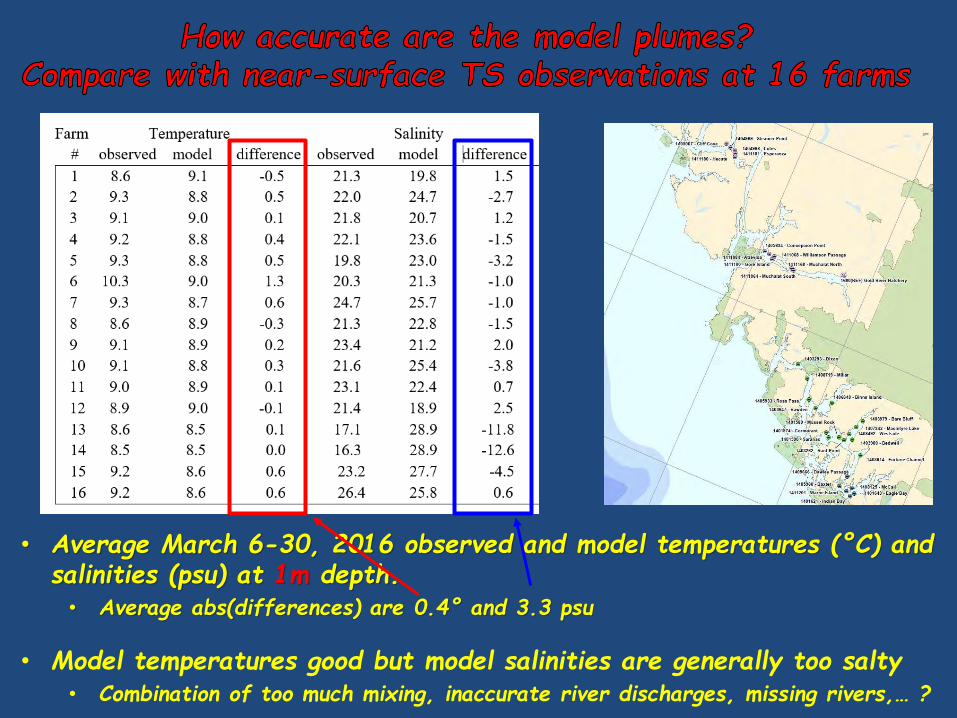
• Average March 6-30, 2016 observed and model temperatures (°C) and salinities (psu) at 1m depth. • Average abs(differences) are 0.4° and 3.3 psu

• Model temperatures good but model salinities are generally too salty• Combination of too much mixing, inaccurate river discharges, missing rivers,… ?

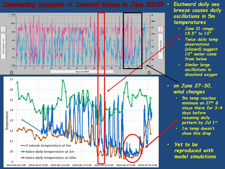
• Eastward daily sea breeze causes daily oscillations in 5m temperatures

• June 21 range: 15.5° to 10°

• Twice daily temp observations (aliased) suggest 10° water came from below

• Similar large oscillations in dissolved oxygen

• on June 27-30, wind changes• 5m temp reaches

minimum on 27th & stays there for 3-4 days before resuming daily pattern by Jul 1st

• 1m temp doesn’t show this drop

• Yet to be reproduced with model simulations

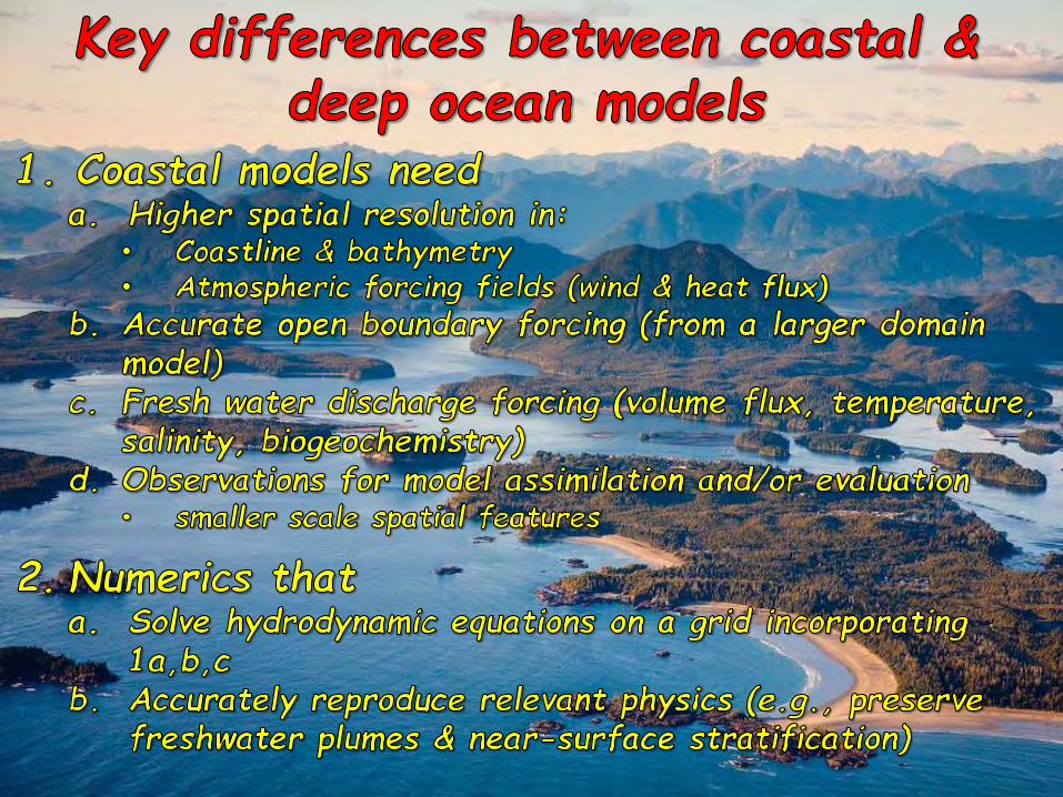
• Coastal ocean modelling has unique challenges/needs:a) Grid that resolves irregular coastlines & variable bathymetry b) High resolution atmospheric forcingc) Accurate open boundary forcingd) Freshwater water discharges (volume flux, temperature, salinity,

biogeochemistry)e) Numerics that can

i. incorporate a) & preferably mudflatsii. accurately reproduce relevant physics

• Interesting (& complex) dynamics:a) Spring-neap variations in estuarine flow, b) Density intrusions, c) Freshwater plumes,d) Internal waves.

• Future work:a) Complete FVCOM simulations for March to July 2016 b) Better simulate & understand “interesting physics” features