
Portfolio optimization in short time horizon
35
Goal Model Approximating the Value function Approximating the optimal investment strategy Example and Numerics Portfolio optimization in short time horizon Rohini Kumar Mathematics Dept., Wayne State University (Joint work with H. Nasralah) WCMF 2017 March 24, 2017 Rohini Kumar Portfolio optimization in short time horizon
Transcript of Portfolio optimization in short time horizon
GoalModel
Approximating the Value functionApproximating the optimal investment strategy
Example and Numerics
Portfolio optimization in short time horizon
Rohini Kumar
Mathematics Dept., Wayne State University(Joint work with H. Nasralah)
WCMF 2017
March 24, 2017
Rohini Kumar Portfolio optimization in short time horizon
GoalModel
Approximating the Value functionApproximating the optimal investment strategy
Example and Numerics
1 Goal
2 ModelIncomplete market - Stochastic volatility modelUtility function
3 Approximating the Value function
4 Approximating the optimal investment strategy
5 Example and Numerics
Rohini Kumar Portfolio optimization in short time horizon
GoalModel
Approximating the Value functionApproximating the optimal investment strategy
Example and Numerics
Objective
Portfolio optimization in a time horizon [t,T ] where τ := T − t → 0.
We want to choose an investment strategy that will maximize theexpected utility of terminal wealth.
We assume a general strictly increasing, concave terminal utilityfunction of wealth UT (x).
Obtain closed-form approximating formulas as τ → 0 of the maximalexpected utility and optimal portfolio.
Rohini Kumar Portfolio optimization in short time horizon
GoalModel
Approximating the Value functionApproximating the optimal investment strategy
Example and Numerics
Literature review
Some recent work where closed-form formulas are obtained in theincomplete market case.
[LS16] “Portfolio Optimization under Local-Stochastic Volatility:Coefficient Taylor Series Approximations & Implied Sharpe Ratio” byLorig and Sircar in 2016
[FSZ13] “Portfolio optimization & stochastic volatility asymptotics”by Fouque, Sircar and Zariphopoulou.
Rohini Kumar Portfolio optimization in short time horizon
GoalModel
Approximating the Value functionApproximating the optimal investment strategy
Example and Numerics
Incomplete market - Stochastic volatility modelUtility function
We work under the assumptions on the market model and utility functionin the 2013 paper “An approximation scheme for solution to the optimalinvestment problem in incomplete markets” by Zariphopoulou andNadtochiy [NZ13].
Rohini Kumar Portfolio optimization in short time horizon
GoalModel
Approximating the Value functionApproximating the optimal investment strategy
Example and Numerics
Incomplete market - Stochastic volatility modelUtility function
Stochastic volatility model for risky asset price
The market consists of one risky asset and one riskless bond. The riskyasset price, St satisfies
dSt = µ(Yt)Stdt + σ(Yt)StdW(1)1t
dYt = b(Yt)dt + a(Yt)(ρdW(1)t +
√1− ρ2dW (2)
t ).
where W (1) and W (2) are independent standard brownian motions,
−1 < ρ < 1. Define λ(y) := µ(y)−rσ(y) where r is the risk-free interest rate.
Rohini Kumar Portfolio optimization in short time horizon
GoalModel
Approximating the Value functionApproximating the optimal investment strategy
Example and Numerics
Incomplete market - Stochastic volatility modelUtility function
Assumptions on stochastic volatility model
Bounded continuous coefficients, volatilities bounded away from zero and|a′|, |a′′|, |b′|, |λ|, |λ′|, |λ′′| are bounded.
Rohini Kumar Portfolio optimization in short time horizon
GoalModel
Approximating the Value functionApproximating the optimal investment strategy
Example and Numerics
Incomplete market - Stochastic volatility modelUtility function
Let πs and π0s denote the discounted amount of wealth invested in the
risky asset and risk-free asset at time s. If x denotes the initial wealth attime t, then the wealth at time s is X t,x,π
s := πs + π0s , which evolves as
dX t,x,πs = σ(Ys)πs(λ(Ys)ds + dW 1
s ), X t,x,πt = x ,
assuming self-financing strategies (πs , π0s ).
Rohini Kumar Portfolio optimization in short time horizon
GoalModel
Approximating the Value functionApproximating the optimal investment strategy
Example and Numerics
Incomplete market - Stochastic volatility modelUtility function
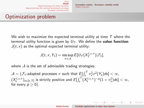
Optimization problem
We wish to maximize the expected terminal utility at time T where theterminal utility function is given by UT . We define the value functionJ(t, x) as the optimal expected terminal utility:
J(t, x ,Yt) = ess supπ∈A
E [UT (X t,x,πT )|Ft ],
where A is the set of admissible trading strategies.
A = {Ft-adapted processes π such that E [∫ T
tπ2s σ
2(Ys)ds] <∞,
(X t,x,πs )s∈[t,T ] is strictly positive and E [
∫ T
t(X t,x,π
s )−p(1 + π2s )ds] <∞,
for every p ≥ 0}.
Rohini Kumar Portfolio optimization in short time horizon
GoalModel
Approximating the Value functionApproximating the optimal investment strategy
Example and Numerics
Incomplete market - Stochastic volatility modelUtility function
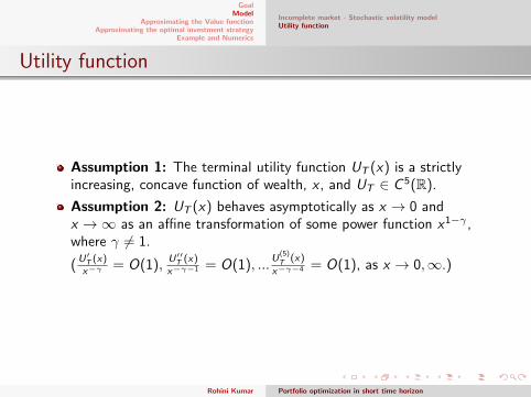
Utility function
Assumption 1: The terminal utility function UT (x) is a strictlyincreasing, concave function of wealth, x , and UT ∈ C 5(R).
Assumption 2: UT (x) behaves asymptotically as x → 0 andx →∞ as an affine transformation of some power function x1−γ ,where γ 6= 1.
(U′T (x)x−γ = O(1),
U′′T (x)x−γ−1 = O(1), ...
U(5)T (x)
x−γ−4 = O(1), as x → 0,∞.)
Rohini Kumar Portfolio optimization in short time horizon
GoalModel
Approximating the Value functionApproximating the optimal investment strategy
Example and Numerics
Incomplete market - Stochastic volatility modelUtility function
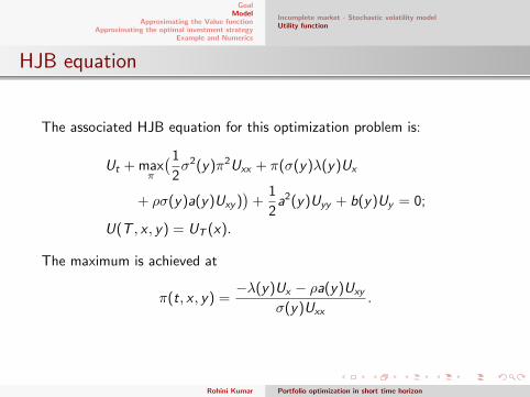
HJB equation
The associated HJB equation for this optimization problem is:
Ut + maxπ
(1
2σ2(y)π2Uxx + π(σ(y)λ(y)Ux
+ ρσ(y)a(y)Uxy ))
+1
2a2(y)Uyy + b(y)Uy = 0;
U(T , x , y) = UT (x).
The maximum is achieved at
π(t, x , y) =−λ(y)Ux − ρa(y)Uxy
σ(y)Uxx.
Rohini Kumar Portfolio optimization in short time horizon
GoalModel
Approximating the Value functionApproximating the optimal investment strategy
Example and Numerics
Incomplete market - Stochastic volatility modelUtility function
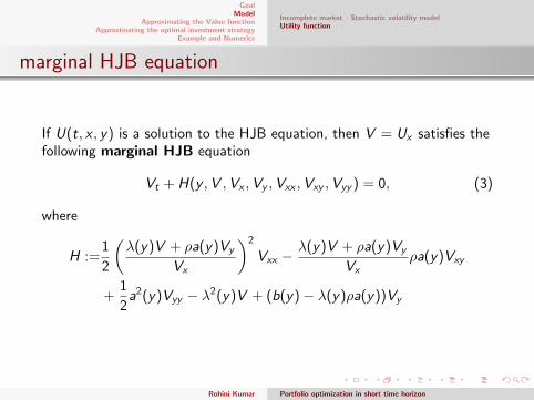
marginal HJB equation
If U(t, x , y) is a solution to the HJB equation, then V = Ux satisfies thefollowing marginal HJB equation
Vt + H(y ,V ,Vx ,Vy ,Vxx ,Vxy ,Vyy ) = 0, (3)
where
H :=1
2
(λ(y)V + ρa(y)Vy
Vx
)2
Vxx −λ(y)V + ρa(y)Vy
Vxρa(y)Vxy
+1
2a2(y)Vyy − λ2(y)V + (b(y)− λ(y)ρa(y))Vy
Rohini Kumar Portfolio optimization in short time horizon
GoalModel
Approximating the Value functionApproximating the optimal investment strategy
Example and Numerics
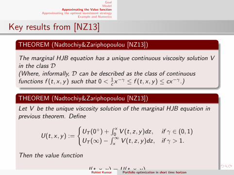
Key results from [NZ13]
THEOREM (Nadtochiy&Zariphopoulou [NZ13])
The marginal HJB equation has a unique continuous viscosity solution Vin the class D(Where, informally, D can be described as the class of continuousfunctions f (t, x , y) such that 0 < 1
c x−γ ≤ f (t, x , y) ≤ cx−γ .)
THEOREM (Nadtochiy&Zariphopoulou [NZ13])
Let V be the unique viscosity solution of the marginal HJB equation inprevious theorem. Define
U(t, x , y) :=
{UT (0+) +
∫ x
0V (t, z , y)dz , if γ ∈ (0, 1)
UT (∞)−∫∞x
V (t, z , y)dz , if γ > 1.
Then the value function
J(t, x , y) = U(t, x , y).Rohini Kumar Portfolio optimization in short time horizon
GoalModel
Approximating the Value functionApproximating the optimal investment strategy
Example and Numerics
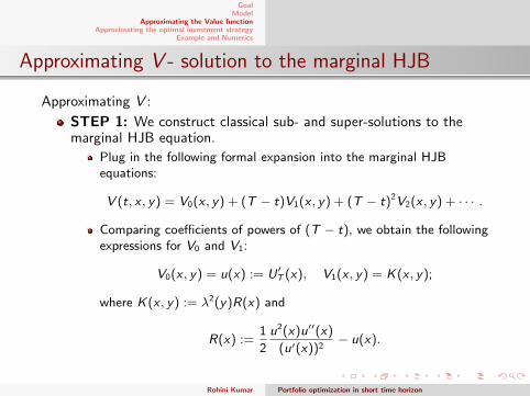
Approximating V - solution to the marginal HJB
Approximating V :
STEP 1: We construct classical sub- and super-solutions to themarginal HJB equation.
Plug in the following formal expansion into the marginal HJBequations:
V (t, x , y) = V0(x , y) + (T − t)V1(x , y) + (T − t)2V2(x , y) + · · · .
Comparing coefficients of powers of (T − t), we obtain the followingexpressions for V0 and V1:
V0(x , y) = u(x) := U ′T (x), V1(x , y) = K(x , y);
where K(x , y) := λ2(y)R(x) and
R(x) :=1
2
u2(x)u′′(x)
(u′(x))2− u(x).
Rohini Kumar Portfolio optimization in short time horizon

GoalModel
Approximating the Value functionApproximating the optimal investment strategy
Example and Numerics
Define V (t, x , y) = u(x) + (T − t)K (x , y)− Cx−γ(T − t)2 andV (t, x , y) = u(x) + (T − t)K (x , y) + Cx−γ(T − t)2, which for anappropriate choice of C > 0 are sub- and super-solutions,respectively, of the marginal HJB equation, i.e.
∂tV + H(V ) ≥ 0 and ∂tV + H(V ) ≤ 0.
Rohini Kumar Portfolio optimization in short time horizon
GoalModel
Approximating the Value functionApproximating the optimal investment strategy
Example and Numerics
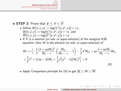
STEP 2: Prove that V ≤ V ≤ V
Define W (t, z , y) := log(V ε(t, ez , y)) + γz ,W (t, z , y) := log(V ε(t, ez , y)) + γz , andW (t, z , y) := log(V
ε(t, ez , y)) + γz
If V is a solution (or sub- or super-solution) of the marginal HJBequation, then W is the solution (or sub- or super-solution) of
Wt + ε[−1
2
(λ+ aρWy )2
Wz − γ
(Wzz
Wz − γ− 1
)− 1
2a2Wyy + aρ
λ+ aρWy
Wz − γWzy
+1
2λ2 + (λaρ− b)Wy +
1
2a2(ρ2 − 1)(Wy )2
]= 0.
(4)
Apply Comparison principle for (4) to get W ≤ W ≤ W .
Rohini Kumar Portfolio optimization in short time horizon
GoalModel
Approximating the Value functionApproximating the optimal investment strategy
Example and Numerics
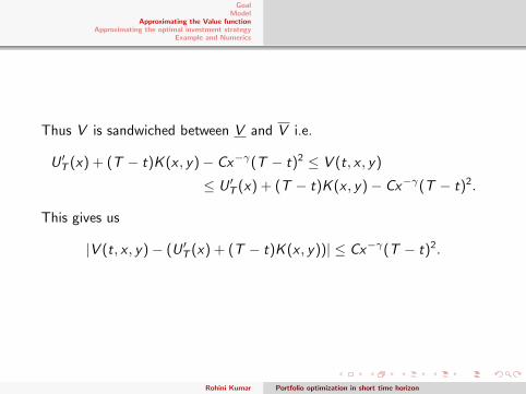
Thus V is sandwiched between V and V i.e.
U ′T (x) + (T − t)K (x , y)− Cx−γ(T − t)2 ≤ V (t, x , y)
≤ U ′T (x) + (T − t)K (x , y)− Cx−γ(T − t)2.
This gives us
|V (t, x , y)− (U ′T (x) + (T − t)K (x , y))| ≤ Cx−γ(T − t)2.
Rohini Kumar Portfolio optimization in short time horizon
GoalModel
Approximating the Value functionApproximating the optimal investment strategy
Example and Numerics
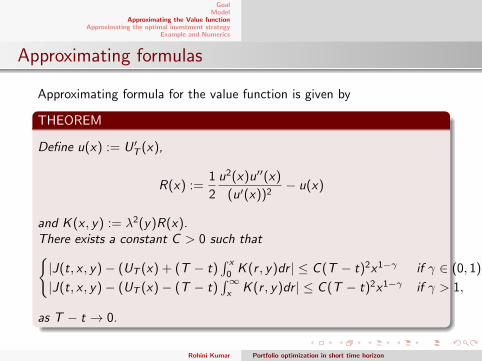
Approximating formulas
Approximating formula for the value function is given by
THEOREM
Define u(x) := U ′T (x),
R(x) :=1
2
u2(x)u′′(x)
(u′(x))2− u(x)
and K (x , y) := λ2(y)R(x).There exists a constant C > 0 such that{|J(t, x , y)− (UT (x) + (T − t)
∫ x
0K (r , y)dr | ≤ C (T − t)2x1−γ if γ ∈ (0, 1),
|J(t, x , y)− (UT (x)− (T − t)∫∞x
K (r , y)dr | ≤ C (T − t)2x1−γ if γ > 1,
as T − t → 0.
Rohini Kumar Portfolio optimization in short time horizon
GoalModel
Approximating the Value functionApproximating the optimal investment strategy
Example and Numerics
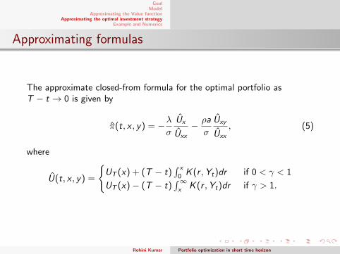
Approximating formulas
The approximate closed-from formula for the optimal portfolio asT − t → 0 is given by
π(t, x , y) = −λσ
Ux
Uxx
− ρa
σ
Uxy
Uxx
, (5)
where
U(t, x , y) =
{UT (x) + (T − t)
∫ x
0K (r ,Yt)dr if 0 < γ < 1
UT (x)− (T − t)∫∞x
K (r ,Yt)dr if γ > 1.
Rohini Kumar Portfolio optimization in short time horizon
GoalModel
Approximating the Value functionApproximating the optimal investment strategy
Example and Numerics
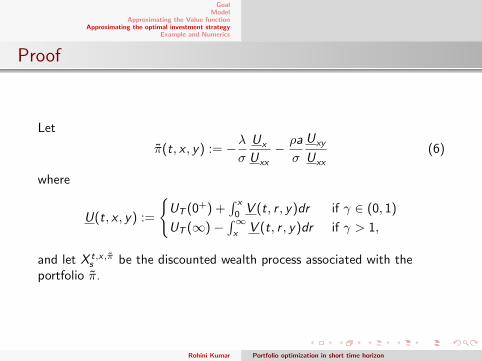
Proof
Let
π(t, x , y) := −λσ
Ux
Uxx
− ρa
σ
Uxy
Uxx
(6)
where
U(t, x , y) :=
{UT (0+) +
∫ x
0V (t, r , y)dr if γ ∈ (0, 1)
UT (∞)−∫∞x
V (t, r , y)dr if γ > 1,
and let X t,x,πs be the discounted wealth process associated with the
portfolio π.
Rohini Kumar Portfolio optimization in short time horizon

GoalModel
Approximating the Value functionApproximating the optimal investment strategy
Example and Numerics
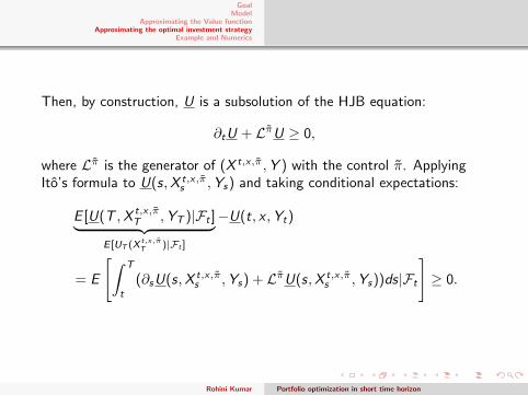
Then, by construction, U is a subsolution of the HJB equation:
∂tU + LπU ≥ 0,
where Lπ is the generator of (X t,x,π,Y ) with the control π.
ApplyingIto’s formula to U(s,X t,x,π
s ,Ys) and taking conditional expectations:
E [U(T ,X t,x,πT ,YT )|Ft ]︸ ︷︷ ︸
E [UT (Xt,x,πT )|Ft ]
−U(t, x ,Yt)
= E
[∫ T
t
(∂sU(s,X t,x,πs ,Ys) + LπU(s,X t,x,π
s ,Ys))ds|Ft
]≥ 0.
Rohini Kumar Portfolio optimization in short time horizon
GoalModel
Approximating the Value functionApproximating the optimal investment strategy
Example and Numerics
Then, by construction, U is a subsolution of the HJB equation:
∂tU + LπU ≥ 0,
where Lπ is the generator of (X t,x,π,Y ) with the control π. ApplyingIto’s formula to U(s,X t,x,π
s ,Ys) and taking conditional expectations:
E [U(T ,X t,x,πT ,YT )|Ft ]︸ ︷︷ ︸
E [UT (Xt,x,πT )|Ft ]
−U(t, x ,Yt)
= E
[∫ T
t
(∂sU(s,X t,x,πs ,Ys) + LπU(s,X t,x,π
s ,Ys))ds|Ft
]≥ 0.
Rohini Kumar Portfolio optimization in short time horizon
GoalModel
Approximating the Value functionApproximating the optimal investment strategy
Example and Numerics
Thus,U(t, x ,Yt) ≤ E [UT (X t,x,π
T )|Ft ] ≤ J(t, x ,Yt).
We know that
|J(t, x , y)− U(t, x , y)| = O((T − t)2)O(x1−γ).
Rohini Kumar Portfolio optimization in short time horizon
GoalModel
Approximating the Value functionApproximating the optimal investment strategy
Example and Numerics
Thus,U(t, x ,Yt) ≤ E [UT (X t,x,π
T )|Ft ] ≤ J(t, x ,Yt).
We know that
|J(t, x , y)− U(t, x , y)| = O((T − t)2)O(x1−γ).
Rohini Kumar Portfolio optimization in short time horizon
GoalModel
Approximating the Value functionApproximating the optimal investment strategy
Example and Numerics
Lemma
For X t,x,πs the wealth process under portfolio π, there exists a c > 0 such
that
|J(t, x ,Yt)− E [UT (X t,x,πT )|Ft ] ≤ c(T − t)2x1−γ , as T − t → 0.
Rohini Kumar Portfolio optimization in short time horizon
GoalModel
Approximating the Value functionApproximating the optimal investment strategy
Example and Numerics
Lemma
For π and π defined in (5) and (6), respectively, we have
|π − π| = O((T − t)2)O(1 + x), as T − t → 0. (7)
Rohini Kumar Portfolio optimization in short time horizon
GoalModel
Approximating the Value functionApproximating the optimal investment strategy
Example and Numerics
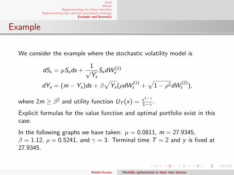
Example
We consider the example where the stochastic volatility model is
dSs = µSsds +1√Ys
SsdW(1)s
dYs = (m − Ys)ds + β√Ys(ρdW
(1)t +
√1− ρ2dW (2)
t ),
where 2m ≥ β2 and utility function UT (x) = x1−γ
1−γ .
Explicit formulas for the value function and optimal portfolio exist in thiscase.
In the following graphs we have taken: µ = 0.0811, m = 27.9345,β = 1.12, ρ = 0.5241, and γ = 3. Terminal time T = 2 and y is fixed at27.9345.
Rohini Kumar Portfolio optimization in short time horizon
GoalModel
Approximating the Value functionApproximating the optimal investment strategy
Example and Numerics
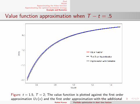
Value function approximation when T − t = .5
Figure: t = 1.5, T = 2; The value function is plotted against the first orderapproximation UT (x) and the first order approximation with the additionalcorrection term. It is difficult to distinguish between the value function and thesecond order approximation.
Rohini Kumar Portfolio optimization in short time horizon
GoalModel
Approximating the Value functionApproximating the optimal investment strategy
Example and Numerics
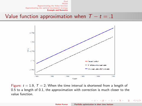
Value function approximation when T − t = .1
Figure: t = 1.9, T = 2; When the time interval is shortened from a length of0.5 to a length of 0.1, the approximation with correction is much closer to thevalue function.
Rohini Kumar Portfolio optimization in short time horizon
GoalModel
Approximating the Value functionApproximating the optimal investment strategy
Example and Numerics
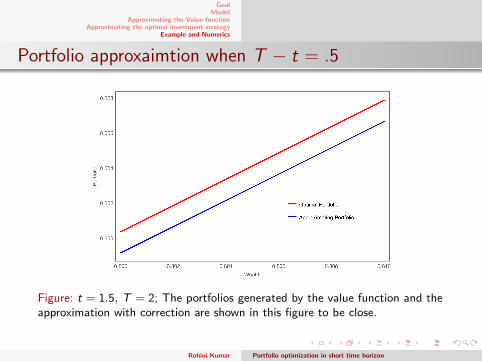
Portfolio approxaimtion when T − t = .5
Figure: t = 1.5, T = 2; The portfolios generated by the value function and theapproximation with correction are shown in this figure to be close.
Rohini Kumar Portfolio optimization in short time horizon
GoalModel
Approximating the Value functionApproximating the optimal investment strategy
Example and Numerics
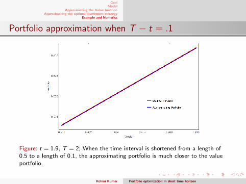
Portfolio approximation when T − t = .1
Figure: t = 1.9, T = 2; When the time interval is shortened from a length of0.5 to a length of 0.1, the approximating portfolio is much closer to the valueportfolio.
Rohini Kumar Portfolio optimization in short time horizon
GoalModel
Approximating the Value functionApproximating the optimal investment strategy
Example and Numerics
References
Portfolio optimization & stochastic volatility asymptotics, Fouque,Jean-Pierre and Sircar, Ronnie and Zariphopoulou, Thaleia, toappear in Mathematical Finance
Portfolio Optimization under Local-Stochastic Volatility: CoefficientTaylor Series Approximations & Implied Sharpe Ratio, Lorig,Matthew and Sircar, Ronnie, SIAM J. Financial Mathematics,volume 7, 2016, pages 418-447
Nadtochiy, Sergey and Zariphopoulou, Thaleia, An approximationscheme for solution to the optimal investment problem in incompletemarkets, SIAM J. Financial Math., 2013, Vol 4, Number 1,p.494-538, http://dx.doi.org/10.1137/120869080
Rohini Kumar Portfolio optimization in short time horizon

GoalModel
Approximating the Value functionApproximating the optimal investment strategy
Example and Numerics
Thank You!
Rohini Kumar Portfolio optimization in short time horizon
GoalModel
Approximating the Value functionApproximating the optimal investment strategy
Example and Numerics
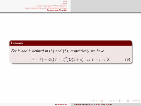
Lemma
For π and π defined in (5) and (6), respectively, we have
|π − π| = O((T − t)2)O(1 + x), as T − t → 0. (9)
Rohini Kumar Portfolio optimization in short time horizon
GoalModel
Approximating the Value functionApproximating the optimal investment strategy
Example and Numerics
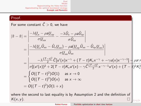
Proof.
For some constant C > 0, we have
|π − π| =
∣∣∣∣∣−λUx − ρaUxy
σUxx
− −λUx − ρaUxy
σUxx
∣∣∣∣∣=
∣∣∣∣∣−λ(Ux Uxx − UxUxx)− ρa(Uxy Uxx − UxyUxx)
σUxx Uxx
∣∣∣∣∣=
∣∣∣∣∣ −λ (T−t)22 C [u′(x)x−γ + (T − t)Kxx
−γ +−γu(x)x−γ−1]− ρaγC (T−t)32 x−γ−1Kxy
σ[(u′(x))2 + 2(T − t)Kxu′(x)− γC (T−t)22 x−γ−1u′(x) + (T − t)2K 2
x − Cγ (T−t)32 x−γ−1Kx ]
∣∣∣∣∣=
{O((T − t)2)O(1) as x → 0
O((T − t)2)O(x) as x →∞
= O((T − t)2)O(1 + x)
where the second to last equality is by Assumption 2 and the definition ofK (x , y).
Rohini Kumar Portfolio optimization in short time horizon