PHYS  507  Lecture  7:  Electrostatics  Special  Techniques:  Part  B

Dr.  Vasileios  Lempesis

Separation  of  Variables  -­‐‑a

•  The method of separation of variables, is applicable in circumstances where the potential (V) or the charge density (σ) is specified on the boundaries of some region, and we are asked to find the potential in the interior. The strategy is:!

•  We look for solutions that are the products of functions, each of which depends on only one of the coordinates. !

•  The success of this method hinged on two extraordinary properties of the separable solutions: completeness and orthogonality.!

Separation  of  Variables  -­‐‑b!

•  A set of functions fn(y) is said to be complete if any other function f(y) can be expressed as a linear combination of them:!

•  A set of functions fn(y) is said to be orthogonal if the integral of the product of any of two different members of the group is zero:!

f (y) = Cn fn (y)n=1

∞

∑

fn (y) fm(y)dy0

a

∫ = 0 for n ≠m

Legendre  Functions •  Legendre   functions   or   Legendre   polynomials   are   the  

solutions   of     Legendre’s   differential   equation   that  appear  when  we  separate   the  variables  of  HelmholE’  equation,   Laplace   equation   or   Schrodinger   equation  using  spherical  coordinate.  

•  They   are   solutions   of   the   following   differential  equation:

• The constant n is an integer (n=0,1,2,…).

•  converge only when !

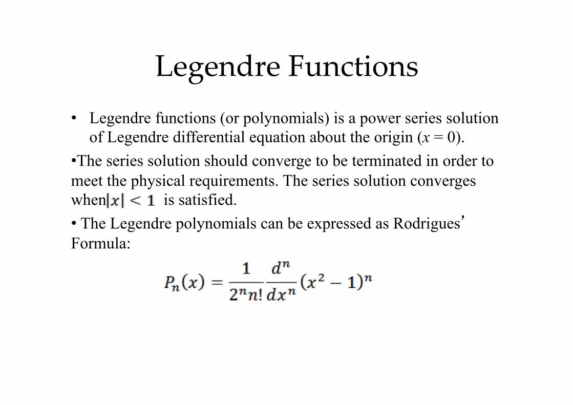
Legendre  Functions  •  Legendre functions (or polynomials) is a power series solution

of Legendre differential equation about the origin (x = 0). • The series solution should converge to be terminated in order to meet the physical requirements. The series solution converges when is satisfied. •  The Legendre polynomials can be expressed as Rodrigues’ Formula:

Legendre  Polynomial  plots

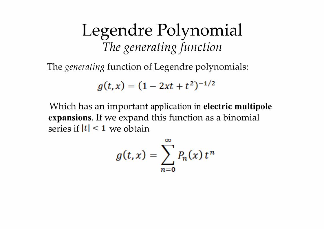
Legendre  Polynomial  The  generating  function

       The  generating  function  of  Legendre  polynomials:          Which  has  an  important  application in electric multipole

expansions.  If  we  expand  this  function  as  a  binomial  series  if                          we  obtain

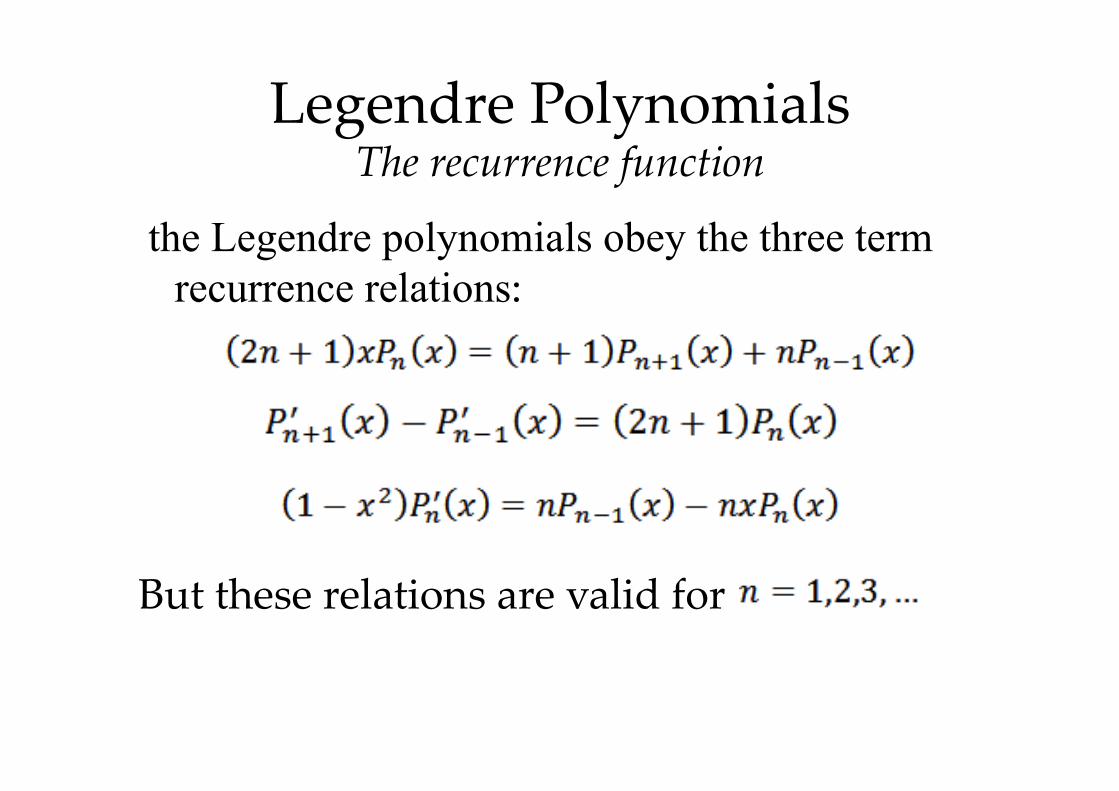
Legendre  Polynomials  The  recurrence  function

 the Legendre polynomials obey the three term recurrence relations:

But  these  relations  are  valid  for

Legendre  Polynomials  Special  Properties  

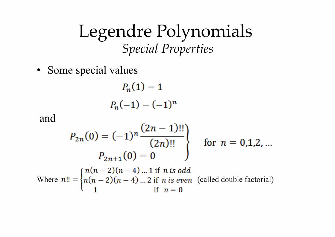
•  Some special values

and Where (called double factorial)

Legendre  Polynomials  Special  Properties  

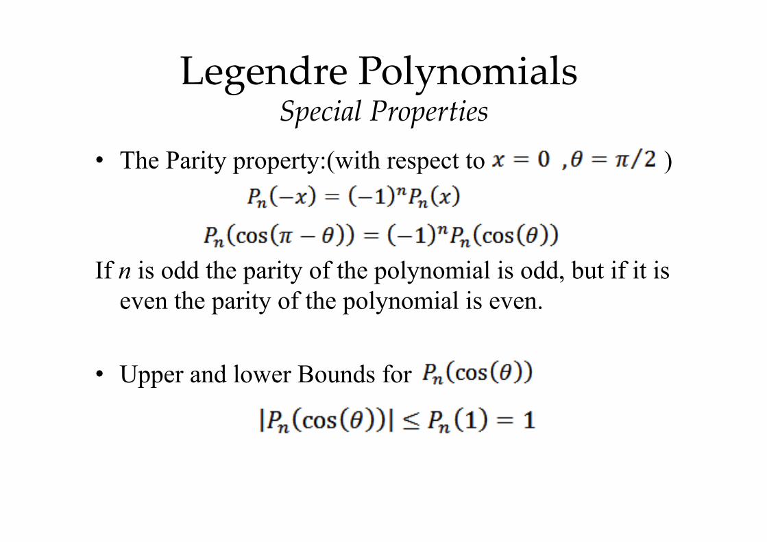
•  The Parity property:(with respect to )

If n is odd the parity of the polynomial is odd, but if it is even the parity of the polynomial is even.

•  Upper and lower Bounds for

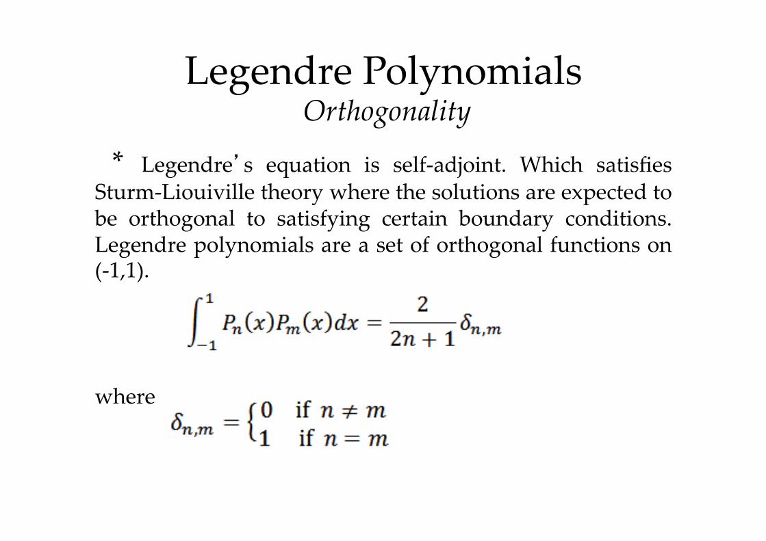
Legendre  Polynomials      Orthogonality

  *   Legendre’s   equation   is   self-­‐‑adjoint.   Which   satisfies  Sturm-­‐‑Liouiville  theory  where  the  solutions  are  expected  to  be   orthogonal   to   satisfying   certain   boundary   conditions.  Legendre  polynomials  are  a  set  of  orthogonal  functions  on  (-­‐‑1,1). where  

Legendre  Polynomials    legendre  Series

•  According to Sturm-Liouville theory that Legendre polynomial form a complete set.

•  The coefficients are obtained by multiplying the series by and integrating in the interval [-1,1]

Multipole Expansion-a"

•  If you are far away from a localized charge distribution of total charge Q then you approximate at large distances the potential with that of a point charge:!

•  But what if this charge is zero? The answer is not as straightforward as it looks. This is where the method of multipole expansion is used in electrostatics.!

V =14πε0

Qr

Multipole Expansion-b"

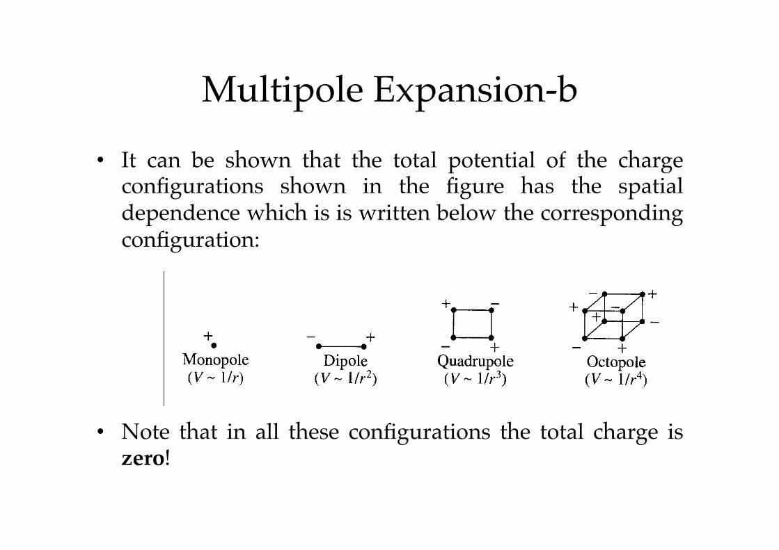
•  It can be shown that the total potential of the charge configurations shown in the figure has the spatial dependence which is is written below the corresponding configuration:!

•  Note that in all these configurations the total charge is zero!!

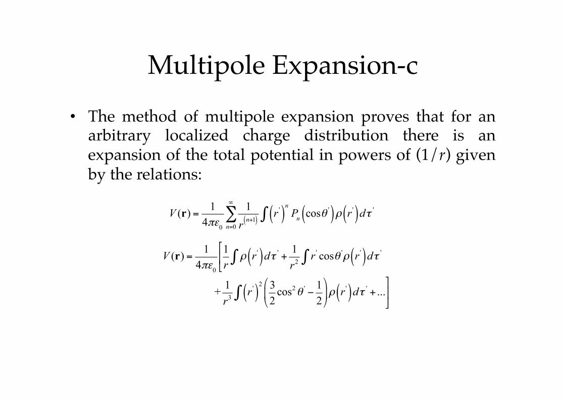
Multipole Expansion-c"

•  The method of multipole expansion proves that for an arbitrary localized charge distribution there is an expansion of the total potential in powers of (1/r) given by the relations:!

V (r) = 14πε0

1

r n+1( )r '( )

nPn cosθ

'( )ρ r '( )dτ '∫n=0

∞

∑

V (r) = 14πε0

1r!

"# ρ r '( )dτ '∫ +

1r2

r ' cosθ 'ρ r '( )dτ '∫

+ 1r3

r '( )2 3

2cos2θ ' −

12

&

'(

)

*+ρ r '( )dτ ' + ...∫

,

-.

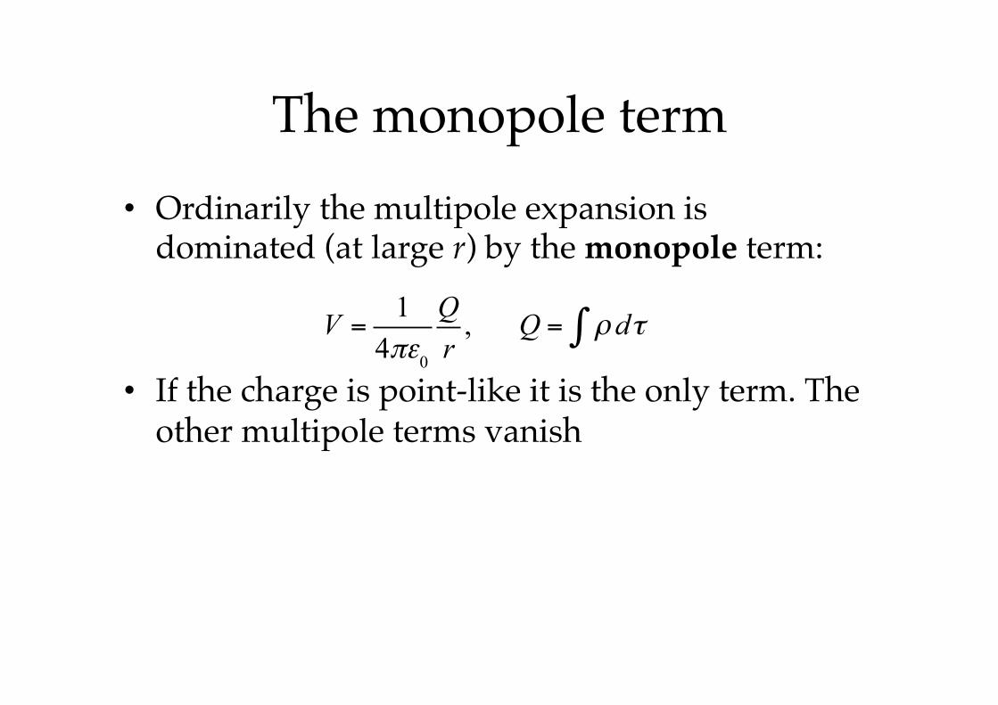
The monopole term  •  Ordinarily the multipole expansion is

dominated (at large r) by the monopole term:!

•  If the charge is point-like it is the only term. The other multipole terms vanish!

V =1

4πε0

Qr

, Q = ρ dτ∫

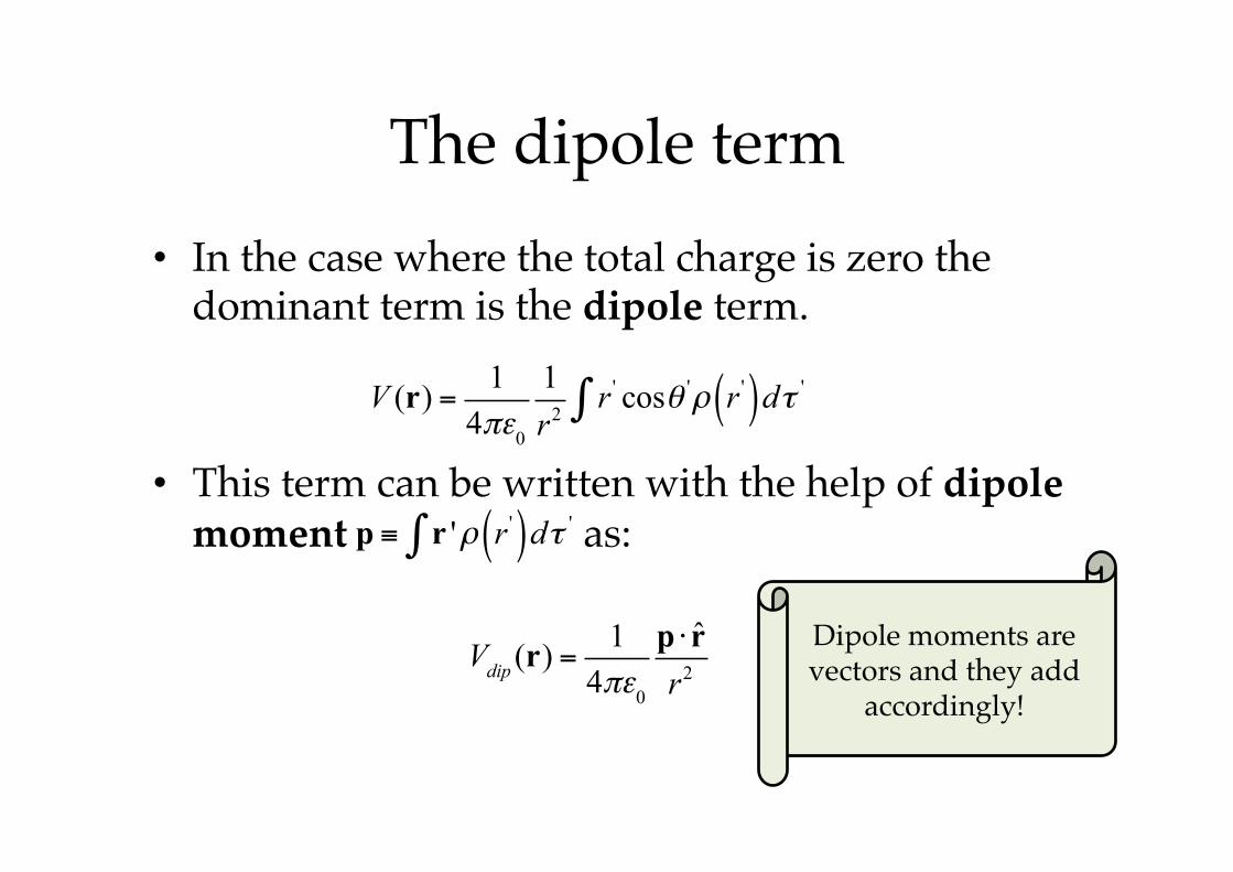
The dipole term  •  In the case where the total charge is zero the

dominant term is the dipole term.!

•  This term can be written with the help of dipole moment as:!

!

V (r) = 14πε0

1r2

r ' cosθ 'ρ r '( )dτ '∫

p ≡ r 'ρ r '( )dτ '∫

Vdip (r) =14πε0

p ⋅ rr2

Dipole moments are vectors and they add

accordingly!!

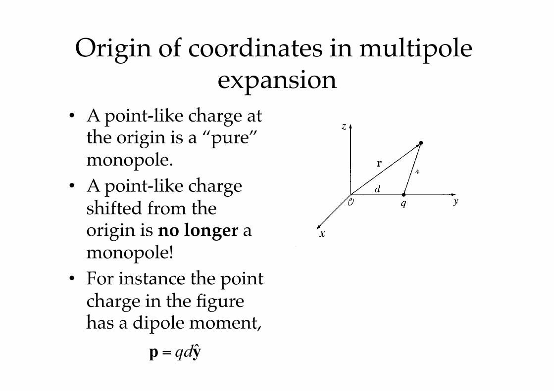
Origin of coordinates in multipole expansion!

•  A point-like charge at the origin is a “pure” monopole.!

•  A point-like charge shifted from the origin is no longer a monopole!!

•  For instance the point charge in the figure has a dipole moment, !

p = qdy